ecosystem vulnerability assessment and … vulnerability assessment and synthesis: a report from the...
TRANSCRIPT
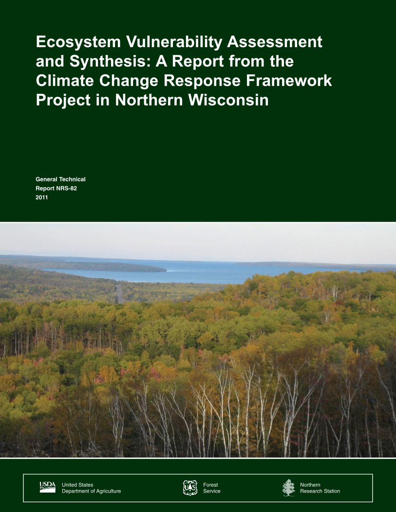
Ecosystem Vulnerability Assessment and Synthesis: A Report from the Climate Change Response Framework Project in Northern Wisconsin
NorthernResearch Station
United States Department of Agriculture
ForestService
General Technical
Report NRS-82
2011
The forests of northern Wisconsin will likely experience dramatic changes over the next 100 years as a result of climate change. This assessment evaluates key forest ecosystem vulnerabilities to climate change across northern Wisconsin under a range of future climate scenarios with a focus on the Chequamegon-Nicolet National Forest. We describe the contemporary landscape and major existing climate trends using state climatological data, as well as potential future climate trends for this region using downscaled global data from general circulation models. We identify potential vulnerabilities by incorporating these future climate projections into species distribution and ecosystem process models and assessing potential changes to northern Wisconsin forests. Warmer temperatures and shifting precipitation patterns are expected to infl uence ecosystem drivers and increase stressors, including more frequent disturbances and increased amount or severity of pests and diseases. Forest ecosystems will continue to adapt to changing conditions. Even under conservative climate change scenarios, suitable habitat for many tree species is expected to move northward. Many species, including balsam fi r, white spruce, paper birch, and quaking aspen, are projected to decline as their suitable habitat decreases in quality and extent. Certain species, communities, and ecosystems may not be particularly resilient to the increases in stress or changes in habitat, and they may be subject to severe declines in abundance or may be lost entirely from the landscape. These include fragmented and static ecosystems, as well as ecosystems containing rare species or species already in decline. Identifying vulnerable species and forests can help landowners, managers, regulators, and policymakers establish priorities for management and monitoring.
Visit our homepage at: http://www.nrs.fs.fed.us/
Published by: For additional copies:
USDA FOREST SERVICE USDA Forest Service11 CAMPUS BLVD., SUITE 200 Publications DistributionNEWTOWN SQUARE, PA 19073-3294 359 Main Road Delaware, OH 43015-8640June 2011 Fax: 740-368-0152
Manuscript received for publication November 2010
Cover PhotoCover photo used with permission of Linda R. Parker, Chequamegon-Nicolet National Forest.
ABSTRACT
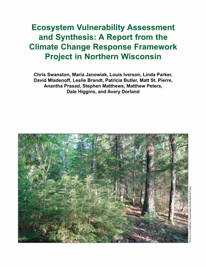
Ecosystem Vulnerability Assessment and Synthesis: A Report from the
Climate Change Response Framework Project in Northern Wisconsin
Chris Swanston, Maria Janowiak, Louis Iverson, Linda Parker, David Mladenoff, Leslie Brandt, Patricia Butler, Matt St. Pierre,
Anantha Prasad, Stephen Matthews, Matthew Peters, Dale Higgins, and Avery Dorland
Pho
to b
y To
m M
atth
iae,
Che
quam
egon
-Nic
olet
Nat
iona
l For
est
CHRIS SWANSTON is a research ecologist with the U.S. Forest Service, Northern Research Station and director of the Northern Institute of Applied Climate Science, 410 MacInnes Drive, Houghton, MI 49931, [email protected]
MARIA JANOWIAK is a climate change adaptation and carbon management scientist with the Northern Institute of Applied Climate Science, 410 MacInnes Drive, Houghton, MI 49931, [email protected]
LOUIS IVERSON is a landscape ecologist with the U.S. Forest Service, Northern Research Station, 359 Main Road, Delaware, OH 43015, [email protected]
LINDA PARKER is a forest ecologist with the U.S. Forest Service, Chequamegon-Nicolet National Forest, 500 Hanson Lake Road, Rhinelander, WI 54501, [email protected]
DAVID MLADENOFF is a professor with the University of Wisconsin, Department of Forest and Wildlife Ecology, 1630 Linden Drive, Madison, WI 53706, [email protected]
LESLIE BRANDT is a climate change specialist with the Northern Institute of Applied Climate Science, 626 East Wisconsin Avenue, Milwaukee, WI 53202, [email protected]
PATRICIA BUTLER is a climate change outreach specialist with the Northern Institute of Applied Climate Science, Michigan Technological University School of Forest Resources and Environmental Science, 1400 Townsend Drive, Houghton, MI 49931, [email protected]
MATT ST. PIERRE is a biologist with the U.S. Forest Service, Chequamegon-Nicolet National Forest, 500 Hanson Lake Road, Rhinelander, WI 54501, [email protected]
ANANTHA PRASAD is an ecologist with the U.S. Forest Service, Northern Research Station, 359 Main Road, Delaware, OH 43015, [email protected]
STEVEN MATTHEWS is an ecologist with the U.S. Forest Service, Northern Research Station, 359 Main Road, Delaware, OH 43015, [email protected]
MATTHEW PETERS is a GIS technician with the U.S. Forest Service, Northern Research Station, 11328 East Quintana Avenue, Mesa, AZ 85212, [email protected]
DALE HIGGINS is a forest hydrologist with the U.S. Forest Service, Chequamegon-Nicolet National Forest, 500 Hanson Lake Road, Rhinelander, WI 54501, [email protected]
AVERY DORLAND is forest geneticist and nursery coordinator with the Wisconsin Department of Natural Resources, 101 South Webster Street, Madison, WI 53707, [email protected]
AUTHORS
PREFACE
This is a fi rst assessment of ecological vulnerabilities in northern Wisconsin, with a focus on the Chequamegon-Nicolet National Forest. It includes new information created in conjunction with this effort and synthesizes previous information. Its primary goal is to inform; it does not make recommendations. This assessment is a fundamental component of the Climate Change Response Framework Project in northern Wisconsin. This project incorporates information and perspectives from numerous sources, compiles strategies and approaches for responding to climate change in forests, provides tools for climate adaptation planning, and initiates boundary-spanning partnerships and communication.
This is the fi rst version of this assessment. Scientifi c understanding of climate change and ecosystem response is rapidly growing. Additionally, ongoing research is being conducted specifi cally to provide expanded information to future versions of this assessment. We expect these future versions of the assessment to refl ect new understandings as well as include results from the ongoing studies.
The scope of this assessment is primarily ecological; it considers ecological vulnerabilities in northern Wisconsin with particular emphasis on tree species. It provides very limited direct consideration of water and wildlife, although these are vital issues. Additionally, because pest and diseases will continue to have profound roles in forest ecology, future modeling exercises will provide insights to their interactions with climate change. Although we provide limited
consideration of ecosystem management implications, this assessment does not provide an analysis of wider human dimensions, such as social, infrastructural, and economic vulnerabilities to climate change. The Wisconsin Initiative on Climate Change Impacts (WICCI) has initiated complementary assessment efforts, providing deeper consideration of many these topics. We have closely collaborated with WICCI, and future versions of this assessment will refl ect the combined fi ndings. The Northern Forest Futures Project, led by the U.S. Forest Service Northern Research Station, is also engaged in modeling to assess climate impacts and forest ecosystem interactions, and results will prove useful in future versions.
The format we adopted for this assessment is that of a single document with highly interdependent chapters. Nonetheless, each chapter bears the imprint of a smaller subgroup of authors. Particular leadership and input was provided by Linda Parker, Leslie Brandt, Patricia Butler, and Matt St. Pierre. Louis Iverson and his team were instrumental in providing and interpreting information from the Climate Change Tree Atlas. Likewise, David Mladenoff greatly assisted synthesis of LANDIS-II modeling work, even while beginning a new project to inform the next version of this assessment. Dan Vimont and Michael Notaro (University of Wisconsin-Madison; WICCI Climate Group) generously provided data, fi gures, and expertise to this assessment. Eric Gustafson (USFS) and Don Waller (UW-Madison) kindly provided formal reviews of the assessment.
Given the uncertainty of future greenhouse gas emissions and related climate change, there is a consequent level of uncertainty in ecosystem change that simply cannot be fully resolved. We have endeavored to consider a range of climate projections, use different vegetation models, and combine the
resulting mixture of information with professional experience to assess ecological implications. Future versions will include more details, but continue to balance the desire for defi nitive and precise predictions with the inherent uncertainties of the issues.
Chris Swanston and Maria JanowiakEditors, Ecosystem Vulnerability and Assessment Synthesis
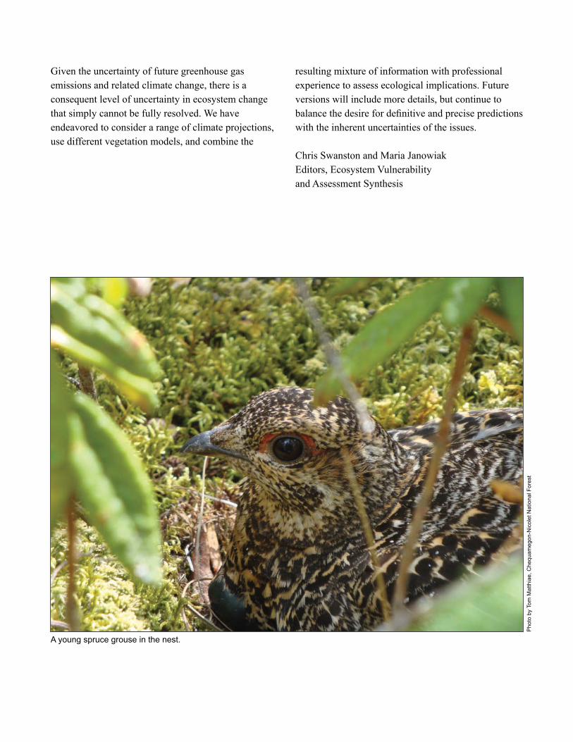
A young spruce grouse in the nest.
Pho
to b
y To
m M
atth
iae,
Che
quam
egon
-Nic
olet
Nat
iona
l For
est
CONTENTS
Executive Summary . . . . . . . . . . . . . . . . . . . . . . . . . . . . . . . . . . . . . . . . .1
Introduction. . . . . . . . . . . . . . . . . . . . . . . . . . . . . . . . . . . . . . . . . . . . . . . .5
Chapter 1: The Contemporary Landscape . . . . . . . . . . . . . . . . . . . . . . . .9
Chapter 2: Climate Change Science and Modeling . . . . . . . . . . . . . . . .31
Chapter 3: Climate Change in Northern Wisconsin . . . . . . . . . . . . . . . .44
Chapter 4: Climate Change Effects on Forests . . . . . . . . . . . . . . . . . . .54
Chapter 5: Implications for Forest Ecosystems . . . . . . . . . . . . . . . . . . .69
Glossary . . . . . . . . . . . . . . . . . . . . . . . . . . . . . . . . . . . . . . . . . . . . . . . . .82
Literature Cited. . . . . . . . . . . . . . . . . . . . . . . . . . . . . . . . . . . . . . . . . . . .88
Appendix 1. . . . . . . . . . . . . . . . . . . . . . . . . . . . . . . . . . . . . . . . . . . . . .105
Appendix 2. . . . . . . . . . . . . . . . . . . . . . . . . . . . . . . . . . . . . . . . . . . . . .106
Appendix 3. . . . . . . . . . . . . . . . . . . . . . . . . . . . . . . . . . . . . . . . . . . . . .109
Appendix 4. Tree Species Vulnerability within Northern Wisconsin Forests to Climate Changes . . . . . . 111
Abbreviations and Acronyms; Units of Measure. . . . . . . . . . . . . . . . . .142
1
EXECUTIVE SUMMARY
Wisconsin is already experiencing the effects of climate change, and impacts are expected to increase in the future. Data gathered from weather stations across Wisconsin indicate that the state has been warming since at least 1950 (Kucharik et al. 2010, WICCI 2009). The length of the growing season has increased by at least 5 days statewide, and up to 20 days in the central and northwest regions of the state. Winters have fewer days below 0 °F (-17 °C) and the nighttime lows and daytime highs have become warmer throughout the year. Lakes freeze later in the year and thaw sooner. Phenological changes consistent with warming have also been observed, including earlier spring blooms and leafout dates.
Although these changes may initially appear to be subtle, they have an increasingly strong ripple effect across northern Wisconsin ecosystems and their many interconnected components and drivers. Many of the most important factors that infl uence forest composition and distribution are expected to change: seasonal temperatures, the timing and type of precipitation, soil moisture, the severity and frequency of natural disturbances, and the range of pests and diseases. As these factors change, the ecosystems themselves are likely to change, often refl ecting an increase in the amount of stress on existing systems.
This assessment was created to evaluate key ecosystem vulnerabilities to climate change across northern Wisconsin under a range of future climate scenarios. We describe the contemporary landscape and present major existing climate trends using state climatological data. We present potential future climate trends for this region using downscaled global data from general circulation models. We incorporated these future climate projections into species distribution and
ecosystem process models to gain understanding of potential changes to northern Wisconsin forests and identify potential vulnerabilities.
The following statements represent our assessment of potential ecosystem responses and vulnerabilities to a range of future climatic changes as presented in Chapters 3 and 4. Though the trends are already established for many of these responses and vulnerabilities, the climate scenarios evaluated are targeted to year 2100. Each assessment statement is followed by our qualitative view of its likelihood of occurring, using specifi c language established by the Intergovernmental Panel on Climate Change (IPCC 2005).
Shifting Stressors
Climate change may relieve some stressors, while exacerbating others. Warmer temperatures and shifting precipitation patterns are expected to strongly infl uence ecosystem drivers.
• Temperatures will increase (virtually certain). Annual increases in temperature represent the broadest possible stressor, strongly infl uencing other stressors and ecosystem responses.
• Growing seasons will get longer (virtually certain). Earlier spring thaws and later fi rst frosts in autumn could result in greater growth and productivity, but only if there is enough water.
• The nature and timing of precipitation will change (virtually certain). Annual precipitation may increase, but a greater proportion of precipitation may occur during winter, leaving longer, drier summers.
2
EXECUTIVE SUMMARY
• Soil moisture patterns will change (virtually certain), with drier soil conditions later in the growing season (likely). Changing rainfall patterns and increased evapotranspiration are expected to decrease soil moisture.
• The frequency, size, and severity of natural disturbances will change across the landscape (very likely). Wind storms, ice storms, droughts, wildfi res, and fl oods are likely to cause greater damage.
• Pests and diseases will increase or become more severe (very likely). Better able to survive warmer winters or complete a second lifecycle in one year, pests may expand their range and abundance.
Ecosystem Response to Shifting Stressors
Forest ecosystems will continue to adapt to changing conditions.
• Suitable habitat for many tree species will move northward (virtually certain). Species at the southern end of their range may experience greater stress as the suitable range moves northward, even as southern and invasive species gain a competitive advantage.
• Many of the current dominant tree species will decline (likely). Many species, including balsam fi r, white spruce, paper birch, and quaking aspen, are projected to decline as their suitable habitat decreases in quality and extent.
• Forest succession will change, making future trajectories unclear (very likely). As species distributions change, communities may fundamentally change or even disaggregate as increased stress, disturbance, and competition from nonnative species alter competitive dynamics.
• Interactions of multiple stressors will reduce forest productivity (likely). Changes in hydrology, disturbances, and other stressors may combine to reduce growth rates, vigor, and health of many important species.
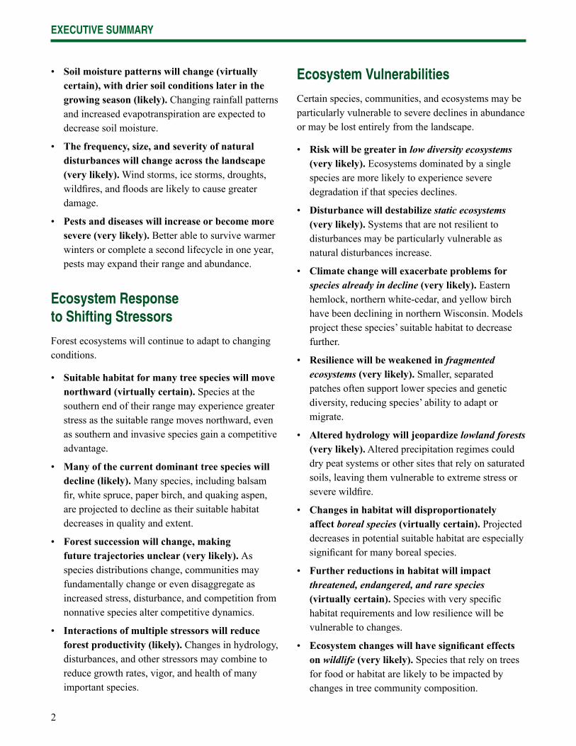
Ecosystem Vulnerabilities
Certain species, communities, and ecosystems may be particularly vulnerable to severe declines in abundance or may be lost entirely from the landscape.
• Risk will be greater in low diversity ecosystems (very likely). Ecosystems dominated by a single species are more likely to experience severe degradation if that species declines.
• Disturbance will destabilize static ecosystems (very likely). Systems that are not resilient to disturbances may be particularly vulnerable as natural disturbances increase.
• Climate change will exacerbate problems for species already in decline (very likely). Eastern hemlock, northern white-cedar, and yellow birch have been declining in northern Wisconsin. Models project these species’ suitable habitat to decrease further.
• Resilience will be weakened in fragmented ecosystems (very likely). Smaller, separated patches often support lower species and genetic diversity, reducing species’ ability to adapt or migrate.
• Altered hydrology will jeopardize lowland forests (very likely). Altered precipitation regimes could dry peat systems or other sites that rely on saturated soils, leaving them vulnerable to extreme stress or severe wildfi re.
• Changes in habitat will disproportionately affect boreal species (virtually certain). Projected decreases in potential suitable habitat are especially signifi cant for many boreal species.
• Further reductions in habitat will impact threatened, endangered, and rare species (virtually certain). Species with very specifi c habitat requirements and low resilience will be vulnerable to changes.
• Ecosystem changes will have signifi cant effects on wildlife (very likely). Species that rely on trees for food or habitat are likely to be impacted by changes in tree community composition.
3
EXECUTIVE SUMMARY
Management Implications
Management practices have always had an important infl uence on forest composition, structure, and function, and will continue to infl uence the way that forests respond to climate change.
• Management will continue to be an important ecosystem driver (virtually certain). Management practices will continue to shape forests by infl uencing forest composition, species movement, and successional trajectories.
• Many current management objectives and practices will face substantial challenges (virtually certain). Many commercially and economically important tree species may face increased stress and lowered productivity, which may affect the availability for some products.
• More resources will be needed to sustain functioning ecosystems (virtually certain). Impacts of climate change will increase the human and capital resources needed to assist regeneration of native species, control wildfi res, combat invasive species, and cope with pests and diseases.
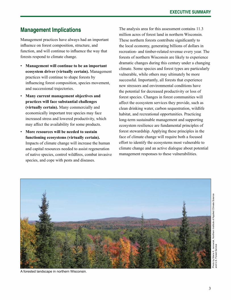
The analysis area for this assessment contains 11.3 million acres of forest land in northern Wisconsin. These northern forests contribute signifi cantly to the local economy, generating billions of dollars in recreation- and timber-related revenue every year. The forests of northern Wisconsin are likely to experience dramatic changes during this century under a changing climate. Some species and forest types are particularly vulnerable, while others may ultimately be more successful. Importantly, all forests that experience new stressors and environmental conditions have the potential for decreased productivity or loss of forest species. Changes in forest communities will affect the ecosystem services they provide, such as clean drinking water, carbon sequestration, wildlife habitat, and recreational opportunities. Practicing long-term sustainable management and supporting ecosystem resilience are fundamental principles of forest stewardship. Applying these principles in the face of climate change will require both a focused effort to identify the ecosystems most vulnerable to climate change and an active dialogue about potential management responses to these vulnerabilities.
A forested landscape in northern Wisconsin.
Pho
to b
y M
aria
K. J
anow
iak,
Nor
ther
n In
stitu
te o
f App
lied
Clim
ate
Sci
ence
an
d U
.S. F
ores
t Ser
vice

4
5
INTRODUCTION
The Intergovernmental Panel on Climate Change has documented and summarized the “unequivocal” evidence for climate change, incorporating information in their analysis from thousands of datasets spanning timescales of decades to millennia (IPCC 2007). Although the nature and severity of future climate change at subregional scales remains uncertain, there is enough information to begin assessing the vulnerability of species and ecosystems across a range of potential future climates. We defi ne vulnerability as “the degree to which a system is susceptible to, and unable to cope with, adverse effects of climate change, including climate variability and extremes” and recognize that a system’s vulnerability is related to the character, magnitude, and rate of climate change and variation that it is exposed to, as well as the system’s sensitivity and capacity to adapt (IPCC 2007). Some forests may exhibit substantial and long-term declines in vigor and productivity as a result of climatic changes; these forests may be considered vulnerable even if they show some resilience in community composition. Other forests are more clearly vulnerable as ecosystem function or community composition is severely altered. The identifi cation of vulnerable species and ecosystems in the near-term is a critical step in long-term planning. Practicing long-term sustainable management and supporting ecosystem resilience are fundamental principles of good stewardship. Applying these principles in the face of climate change will require a focused effort to identify the ecosystems at greatest risk and an active dialogue about potential management responses to the risk.
Context
This assessment is part of a larger effort in northern Wisconsin called the Climate Change Response Framework Project. The project, initiated in 2009, incorporates information and expertise from a wide variety of scientists and land managers to help identify specifi c challenges posed by the changing climate, as well as our potential responses. It was commissioned by the U.S. Forest Service to address the need for information and tools regarding climate change impacts and adaptation. The Chequamegon-Nicolet National Forest (CNNF) was identifi ed as a pilot landscape, and generously supplied ecological and management expertise to the assessment process and overall effort. The Wisconsin Initiative on Climate Change Impacts was also a major contributor of ideas and information to this assessment and the entire project. The project addresses four major questions:
What parts of the northern Wisconsin are most vulnerable to the effects of climate change? This assessment addresses this question by compiling a variety of information to inform land managers in northern Wisconsin about the ecosystem components that are most vulnerable to change under a variety of future climate scenarios.
What options exist to mitigate climate change? A mitigation assessment is underway to describe options for increasing carbon stocks in forests and wood products, increasing the use of wood for bioenergy, and engaging in greenhouse gas markets and registries.
6
INTRODUCTION
How can land managers in northern Wisconsin work together to respond to climate change? A Shared Landscapes Initiative is currently underway to encourage local forest owners and managers and the public to discuss the potential ecological and management pressures associated with climate change and to evaluate opportunities for ongoing discussions and effective ecosystem management partnerships.
How can the latest science be applied to on-the-ground activities? The project is producing a document called Forest Adaptation Resources (FAR): Climate Change Tools and Approaches for Land Managers. FAR includes adaption strategies and approaches, as well as a workbook to apply them in conjunction with this assessment in order to design place-based tactics for climate change adaptation. Additionally, the project established a climate change science roundtable to improve the rapid incorporation of science and monitoring information into management activities. The roundtable supports an ongoing forum for scientists and managers to discuss climate change science needs, applications of science, and monitoring methods.
Scope and Goals
The primary goal of this assessment is to summarize potential changes to the forest ecosystems of northern Wisconsin under a range of future climates, and thereby identify species and ecosystems that may be vulnerable. Included is a synthesis of information about the current landscape as well as projections of climate and vegetation changes used to assess these vulnerabilities. Uncertainties and gaps in understanding are discussed throughout the document.
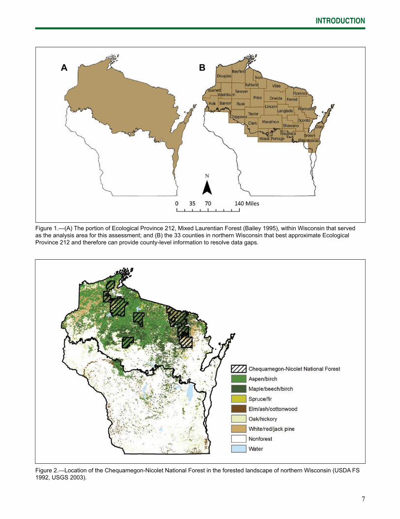
This assessment covers 18.5 million acres of northern Wisconsin within Ecological Province 212 (Mixed Laurentian Forest) of the National Hierarchical Framework of Ecological Units (Bailey 1995, ECOMAP 1993). Under this hierarchy, ecological units are distinguished from one another by major
regional climatic regimes and physical geography. This geographic scope defi nes the analysis area used for much of this document (Fig. 1). We used county-level information that most closely represented the analysis area when ecoregional data were not available (Fig. 1), limiting our selections to the 33 counties that are most analogous to the area within Ecological Province 212: Ashland, Barron, Bayfi eld, Brown, Burnett, Chippewa, Clark, Door, Douglas, Florence, Forest, Iron, Kewaunee, Langlade, Lincoln, Manitowoc, Marathon, Marinette, Menominee, Oconto, Oneida, Outagamie, Polk, Portage, Price, Rusk, Sawyer, Shawano, Taylor, Vilas, Washburn, Waupaca, and Wood.
The CNNF encompasses nearly 1.5 million acres within the analysis area and includes all of the major forest types (Fig. 2). Supplementary information specifi c to the CNNF was used when available and relevant to the broader landscape. Although the CNNF receives some additional focus, this assessment synthesizes information covering all of northern Wisconsin in recognition of the area’s dispersed patterns of forest composition and land ownership.
Assessment Chapters
Chapter 1: The Contemporary Landscape describes existing conditions, providing background on the physical environment, ecological character, and social dimensions of northern Wisconsin.
Chapter 2: Climate Change Science and Modeling contains background on climate change science, projection models, and impact models. It also describes the techniques used in developing climate projections to provide context for the model results presented in later chapters.
Chapter 3: Climate Change in Northern Wisconsin provides information on the past and current climate of northern Wisconsin, as well as projected changes provided by the Climate Working Group of the Wisconsin Initiative on Climate Change Impacts.
7
INTRODUCTION
Figure 1.—(A) The portion of Ecological Province 212, Mixed Laurentian Forest (Bailey 1995), within Wisconsin that served as the analysis area for this assessment; and (B) the 33 counties in northern Wisconsin that best approximate Ecological Province 212 and therefore can provide county-level information to resolve data gaps.
A B
Figure 2.—Location of the Chequamegon-Nicolet National Forest in the forested landscape of northern Wisconsin (USDA FS 1992, USGS 2003).
8
INTRODUCTION
Chapter 4: Climate Change Effects on Forests summarizes results of modeling climate change effects on species distribution and forest ecosystem processes. Two different modeling approaches were used to model climate change impacts on forests, a species distribution model (the Climate Change Tree Atlas) and a process model (LANDIS-II).
Chapter 5: Implications for Forest Ecosystems synthesizes the potential effects of climate change on the ecosystems of northern Wisconsin and outlines key changes to ecosystem stressors, responses to those stressors, and vulnerabilities.
Morning on a lake.
Pho
to b
y Li
nda
R. P
arke
r, C
hequ
ameg
on-N
icol
et N
atio
nal F
ores
t
9
CHAPTER 1: THE CONTEMPORARY LANDSCAPE
The contemporary landscape of northern Wisconsin results from numerous physical, ecological, economic, and social factors. This chapter includes a brief introduction to the complex variables that make up Wisconsin’s northern forests and provides context for the modeling results and interpretations provided in Chapters 4 and 5.
Physical Environment
The physical environment of northern Wisconsin is the result of climate, soil, water, geology, landform, and time. The climate of the region has generally favored forests. It is not as cold as northern Minnesota where boreal forests are dominant, nor is it as dry as areas farther south and west, where grasslands are favored (Mladenoff et al. 2008). In fact, northern Wisconsin possesses a convergence of three major biomes; eastern deciduous forest in the south gives way to boreal forest in the north, and tallgrass prairie persists to the south and west, primarily in isolated remnants. A wide variety of landscapes support these biomes, further adding to the diversity of northern Wisconsin’s landscape.
Climate
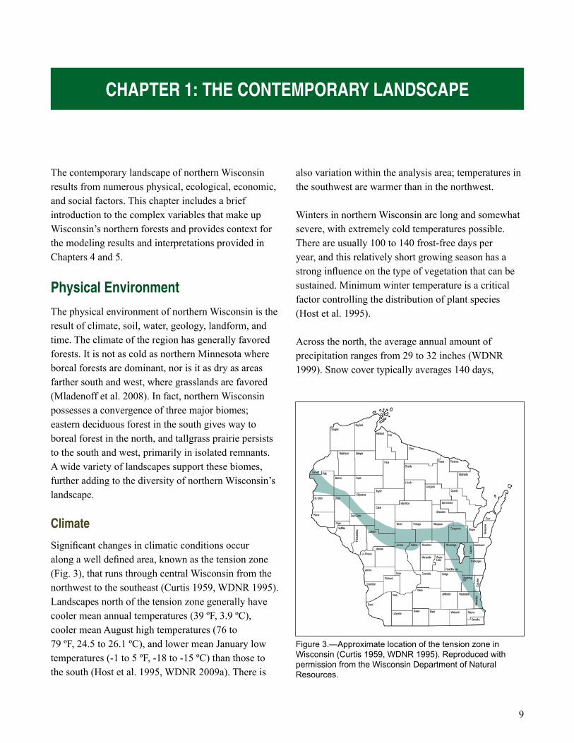
Signifi cant changes in climatic conditions occur along a well defi ned area, known as the tension zone (Fig. 3), that runs through central Wisconsin from the northwest to the southeast (Curtis 1959, WDNR 1995). Landscapes north of the tension zone generally have cooler mean annual temperatures (39 ºF, 3.9 ºC), cooler mean August high temperatures (76 to 79 ºF, 24.5 to 26.1 ºC), and lower mean January low temperatures (-1 to 5 ºF, -18 to -15 ºC) than those to the south (Host et al. 1995, WDNR 2009a). There is
also variation within the analysis area; temperatures in the southwest are warmer than in the northwest.
Winters in northern Wisconsin are long and somewhat severe, with extremely cold temperatures possible. There are usually 100 to 140 frost-free days per year, and this relatively short growing season has a strong infl uence on the type of vegetation that can be sustained. Minimum winter temperature is a critical factor controlling the distribution of plant species (Host et al. 1995).
Across the north, the average annual amount of precipitation ranges from 29 to 32 inches (WDNR 1999). Snow cover typically averages 140 days,
Figure 3.—Approximate location of the tension zone in Wisconsin (Curtis 1959, WDNR 1995). Reproduced with permission from the Wisconsin Department of Natural Resources.
10
CHAPTER 1: THE CONTEMPORARY LANDSCAPE
compared to 65 days in southern Wisconsin (NOAA 2006). A signifi cant lake-effect along Lakes Superior and Michigan produces temperatures that are warmer in autumn and cooler in the spring than inland areas at the same latitude. Moisture-laden air from Lake Superior often rises rapidly over nearby uplands, resulting in heavy precipitation (Albert et al. 1986). Northern Iron County typically receives 100 inches of snow a year, more than any other area in Wisconsin.
Chapter 3 provides more details on historical climate, current climate trends, and projected climatic trends for northern Wisconsin.
Geology and Landform
Bedrock geology in northern Wisconsin is largely formed by Precambrian rock that is more than 600 million years old (Ostrum 1981). Bedrock outcrops are relatively uncommon, although they can be biologically signifi cant for a number of rare plants (such as at the Penokee-Gogebic Range). The surface geology is the result of Pleistocene glaciations.
Glacial ice modifi ed the land surface as it retreated over bedrock of igneous rock, sedimentary rock, limestone, and sandstone; leaving behind a wide variety of landforms, huge deposits of glacial debris, and the depressions which would become lakes and wetlands (Stearns 1987). The most prominent glacial landforms are moraines, till plains, outwash plains, drainage channels, drumlin fi elds, eskers, ice-walled lake plains, extinct glacial lakes, and kettle lakes. Glacial activity also created a globally signifi cant concentration of lakes and an abundance of wetlands (WDNR 2009a).
Soils
Glacial deposits of coarse outwash sands, fi ne-textured clays, and tills serve as the parent material for the soils in of northern Wisconsin. These soils, by comparison,
are less productive than soils found in southern Wisconsin. Hole (1968) described and mapped the soil regions of Wisconsin. Clay soils largely line the shores of Lake Superior. A large peninsula of sandy outwash soils extends from Grantsburg in Burnett County through the Bayfi eld County Peninsula. Other large areas of outwash sands are found in Vilas, Oneida, Marinette, and eastern Florence Counties. Rich silty soils dominate portions of Sawyer, Price, Rusk, Taylor and Marathon Counties. Loamy soils are widespread throughout the area, but are especially common in the northeast counties of Forest and Langlade.
Soils on the Chequamegon-Nicolet National Forest—Medium-productivity sandy loam soils are widespread on the CNNF; they cover 34 percent of the land base. Wetland and organic soils (28 percent), highly productive silt loams (22 percent), and low productivity sand-dominated soils (16 percent) cover the remainder (USDA FS 1998d). The depth of sediments over bedrock ranges from 0 to 393 feet and averages more than 48 feet. Change in elevation exceeds 300 meters and varies by landform. Generally, the topography is level to rolling with 5 to 20 percent slopes, with some areas hilly to very steep (greater than 35 percent).
Wet mineral and organic soils occur on about 424,000 acres (28 percent of the Forest). These wetlands, in varying sizes and shapes, are scattered throughout the landscape but primarily concentrated at lower elevations in old glacial drainage ways and kettles. Wetland soils, which vary from 1 to 32 percent of individual Landtype Associations, are primarily acid-to-neutral peats and mucks that formed from the remains of woody and herbaceous plants (USDA FS 1998d).
11
CHAPTER 1: THE CONTEMPORARY LANDSCAPE
Hydrology
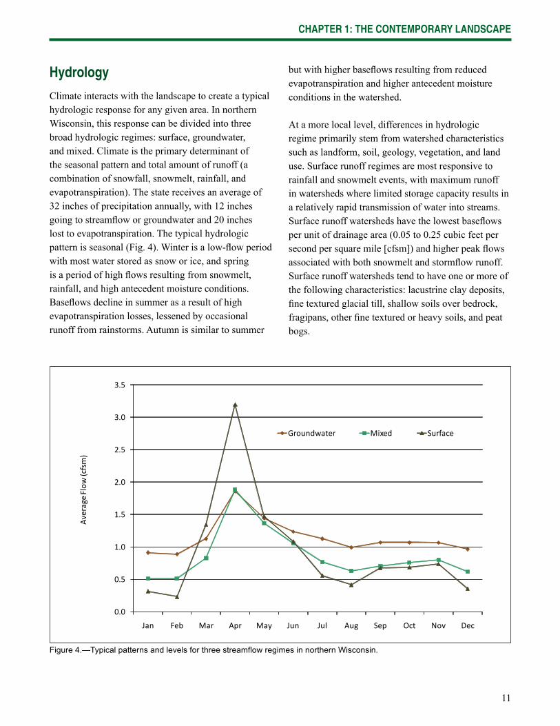
Climate interacts with the landscape to create a typical hydrologic response for any given area. In northern Wisconsin, this response can be divided into three broad hydrologic regimes: surface, groundwater, and mixed. Climate is the primary determinant of the seasonal pattern and total amount of runoff (a combination of snowfall, snowmelt, rainfall, and evapotranspiration). The state receives an average of 32 inches of precipitation annually, with 12 inches going to streamfl ow or groundwater and 20 inches lost to evapotranspiration. The typical hydrologic pattern is seasonal (Fig. 4). Winter is a low-fl ow period with most water stored as snow or ice, and spring is a period of high fl ows resulting from snowmelt, rainfall, and high antecedent moisture conditions. Basefl ows decline in summer as a result of high evapotranspiration losses, lessened by occasional runoff from rainstorms. Autumn is similar to summer
but with higher basefl ows resulting from reduced evapotranspiration and higher antecedent moisture conditions in the watershed.
At a more local level, differences in hydrologic regime primarily stem from watershed characteristics such as landform, soil, geology, vegetation, and land use. Surface runoff regimes are most responsive to rainfall and snowmelt events, with maximum runoff in watersheds where limited storage capacity results in a relatively rapid transmission of water into streams. Surface runoff watersheds have the lowest basefl ows per unit of drainage area (0.05 to 0.25 cubic feet per second per square mile [cfsm]) and higher peak fl ows associated with both snowmelt and stormfl ow runoff. Surface runoff watersheds tend to have one or more of the following characteristics: lacustrine clay deposits, fi ne textured glacial till, shallow soils over bedrock, fragipans, other fi ne textured or heavy soils, and peat bogs.
0.0
0.5
1.0
1.5
2.0
2.5
3.0
3.5
Jan Feb Mar Apr May Jun Jul Aug Sep Oct Nov Dec
Average
Flow
(cfsm)
Groundwater Mixed Surface
Figure 4.—Typical patterns and levels for three streamfl ow regimes in northern Wisconsin.
12
CHAPTER 1: THE CONTEMPORARY LANDSCAPE
Groundwater runoff regimes are least responsive to surface runoff from storms or snowmelt and have high, stable basefl ows (0.5 to 1.0 cfsm) fed by a continuous supply of groundwater. Watersheds with groundwater runoff regimes generally have coarse textured glacial outwash or till that favors groundwater recharge and fen-type wetlands that discharge groundwater. They also tend to have suffi cient elevational relief to produce a steady fl ow of groundwater from uplands to streams. Mixed runoff watersheds typically have landform and soil characteristics that are intermediate between the surface and groundwater regimes, and basefl ows ranging from 0.25 to 0.5 cfsm.
Flood fl ows in northern Wisconsin tend to be relatively low because of the area’s high storage capacity in the form of wetlands and lakes, gentle relief, and soils with high infi ltration capacity. Exceptions include: the clay plains along Lakes Superior and Michigan which have low infi ltration capacity, less storage, and steep slopes in some locations; the Penokee-Gogebic range with shallow soils over bedrock and steeper slopes; and areas of fi ne textured till with low infi ltration capacity. Across much of northern Wisconsin, 100-year fl oods (1.0 percent chance of being exceeded in any given year) typically range from 6 to 33 cfsm and 2-year fl oods (66.7 percent chance of being exceeded in any given year) from 2.6 to 12.7 cfsm (Walker and Krug 2003). In those watersheds with higher fl ood fl ow rates, 100-year fl oods tend to range from 40 to 220 cfsm and 2-year fl oods from 13 to 40 cfsm. Annual fl ood peaks in northern Wisconsin are caused by both snowmelt and rainfall runoff in about equal proportions.
Ecosystem Composition
Northern Wisconsin’s position at the intersection of the eastern deciduous forest biome and the boreal forest biome creates a complex and somewhat unique set of ecological conditions. A major change in vegetation occurs along the tension zone (Fig. 4), where the open landscape of the south (once prairie and oak savanna
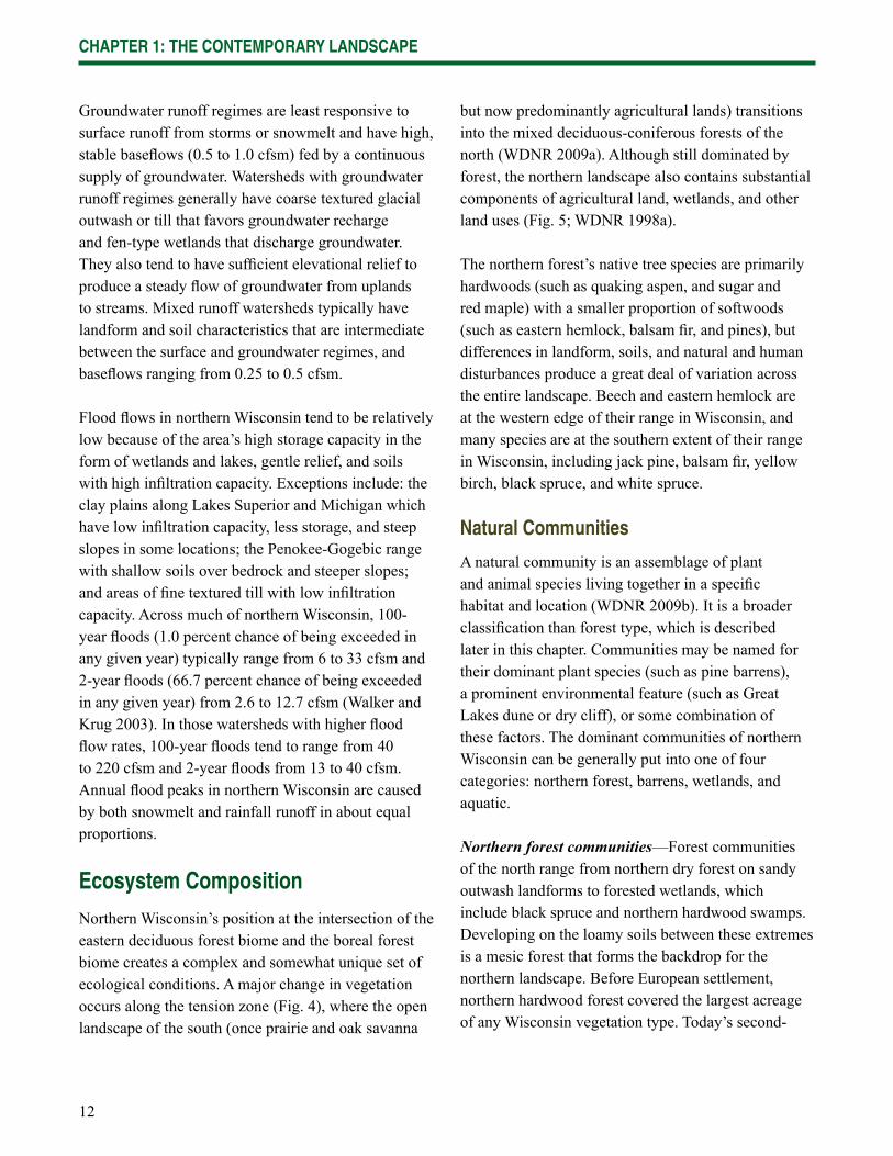
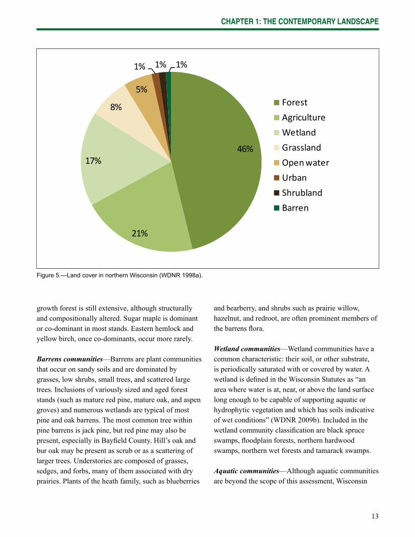
but now predominantly agricultural lands) transitions into the mixed deciduous-coniferous forests of the north (WDNR 2009a). Although still dominated by forest, the northern landscape also contains substantial components of agricultural land, wetlands, and other land uses (Fig. 5; WDNR 1998a).
The northern forest’s native tree species are primarily hardwoods (such as quaking aspen, and sugar and red maple) with a smaller proportion of softwoods (such as eastern hemlock, balsam fi r, and pines), but differences in landform, soils, and natural and human disturbances produce a great deal of variation across the entire landscape. Beech and eastern hemlock are at the western edge of their range in Wisconsin, and many species are at the southern extent of their range in Wisconsin, including jack pine, balsam fi r, yellow birch, black spruce, and white spruce.
Natural Communities
A natural community is an assemblage of plant and animal species living together in a specifi c habitat and location (WDNR 2009b). It is a broader classifi cation than forest type, which is described later in this chapter. Communities may be named for their dominant plant species (such as pine barrens), a prominent environmental feature (such as Great Lakes dune or dry cliff), or some combination of these factors. The dominant communities of northern Wisconsin can be generally put into one of four categories: northern forest, barrens, wetlands, and aquatic.
Northern forest communities—Forest communities of the north range from northern dry forest on sandy outwash landforms to forested wetlands, which include black spruce and northern hardwood swamps. Developing on the loamy soils between these extremes is a mesic forest that forms the backdrop for the northern landscape. Before European settlement, northern hardwood forest covered the largest acreage of any Wisconsin vegetation type. Today’s second-
13
CHAPTER 1: THE CONTEMPORARY LANDSCAPE
46%
21%
17%
8%
5%
1% 1% 1%
Forest
Agriculture
Wetland
Grassland
Openwater
Urban
Shrubland
Barren
Figure 5.—Land cover in northern Wisconsin (WDNR 1998a).
growth forest is still extensive, although structurally and compositionally altered. Sugar maple is dominant or co-dominant in most stands. Eastern hemlock and yellow birch, once co-dominants, occur more rarely.
Barrens communities—Barrens are plant communities that occur on sandy soils and are dominated by grasses, low shrubs, small trees, and scattered large trees. Inclusions of variously sized and aged forest stands (such as mature red pine, mature oak, and aspen groves) and numerous wetlands are typical of most pine and oak barrens. The most common tree within pine barrens is jack pine, but red pine may also be present, especially in Bayfi eld County. Hill’s oak and bur oak may be present as scrub or as a scattering of larger trees. Understories are composed of grasses, sedges, and forbs, many of them associated with dry prairies. Plants of the heath family, such as blueberries
and bearberry, and shrubs such as prairie willow, hazelnut, and redroot, are often prominent members of the barrens fl ora.
Wetland communities—Wetland communities have a common characteristic: their soil, or other substrate, is periodically saturated with or covered by water. A wetland is defi ned in the Wisconsin Statutes as “an area where water is at, near, or above the land surface long enough to be capable of supporting aquatic or hydrophytic vegetation and which has soils indicative of wet conditions” (WDNR 2009b). Included in the wetland community classifi cation are black spruce swamps, fl oodplain forests, northern hardwood swamps, northern wet forests and tamarack swamps.
Aquatic communities—Although aquatic communities are beyond the scope of this assessment, Wisconsin
14
CHAPTER 1: THE CONTEMPORARY LANDSCAPE
has a large and diverse aquatic resource that supports numerous species, communities, ecological processes, and human uses. In addition, many terrestrial species and processes are dependent on neighboring aquatic systems.
Forest Composition and Abundance
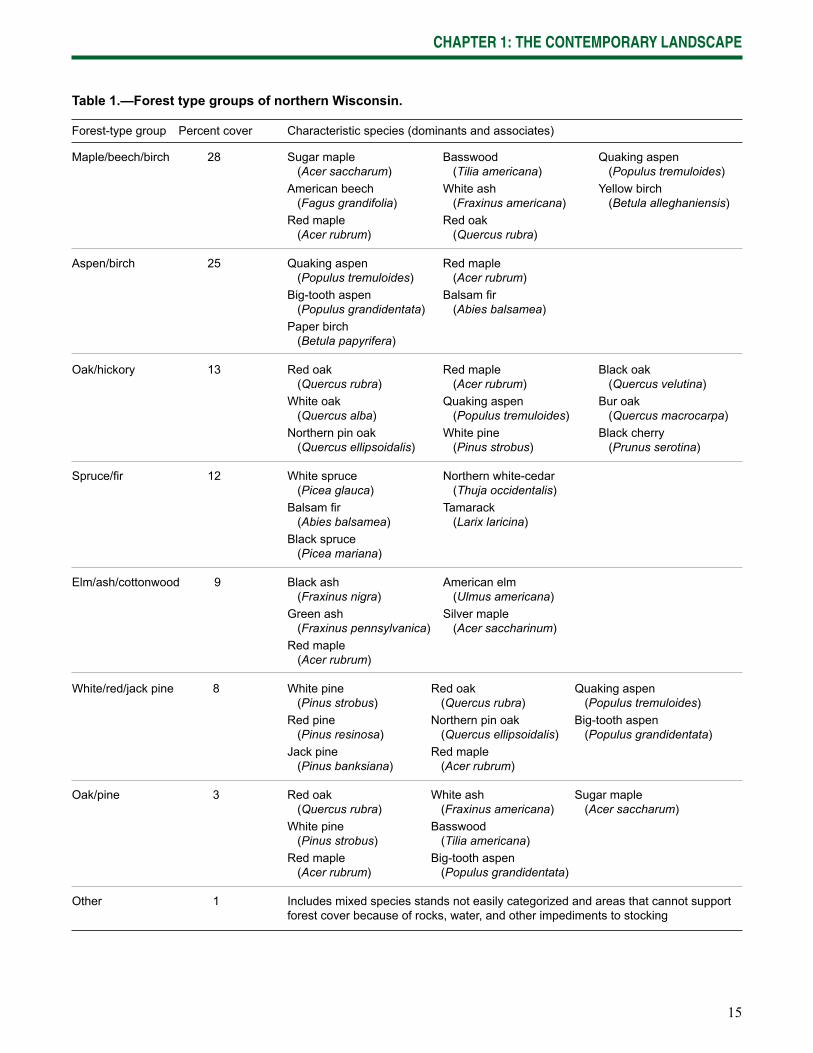
Many forest types are present in the 11.3 million acres of forest land in the analysis area (FIA 2010). Organizations defi ne these forests using different classifi cation systems. This assessment uses two classifi cation systems: one designed by the USDA Forest Service Forest Inventory and Analysis (FIA) program, and another system of species and species associations used by CNNF. Estimates of forest characteristics by acres, type of ownership, and volume of timber by forest-type group were determined using the FIA data, which are derived from permanent plots across the United States (Miles 2010). On the scale of northern Wisconsin, these data reasonably refl ect the forests that are present. However, when studying smaller areas, it is possible to provide data using forest types, which are more specifi c to this region. Using the same forest classifi cation system as the CNNF also facilitates ease of communication and data sharing. Even so, these systems use similar groupings, though by different names. For example, the FIA maple/beech/birch forest-type group is largely synonymous with the CNNF northern hardwood forest type (though in Wisconsin, beech is present only in the eastern counties along Lake Michigan), and the FIA elm/ash/cottonwood forest-type group encompasses the CNNF lowland hardwood forest type.
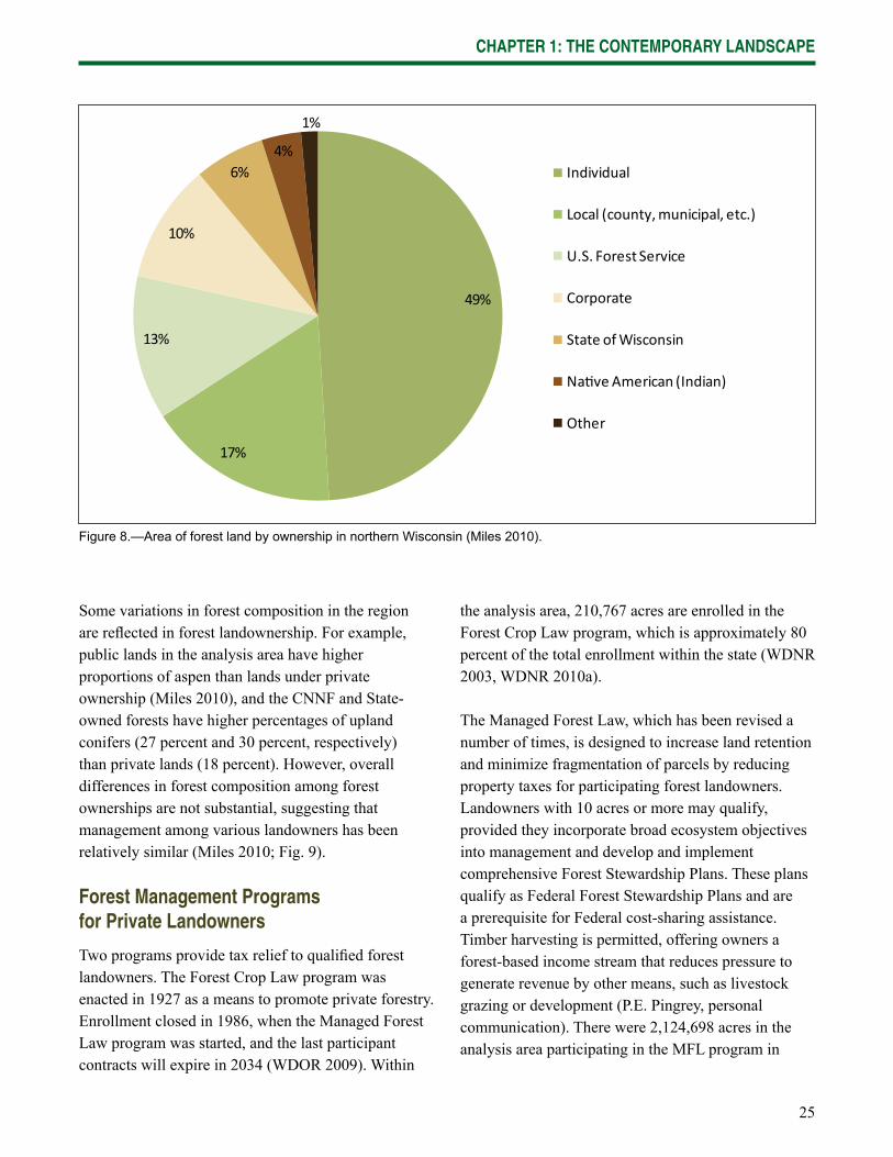
Across northern Wisconsin, maple/beech/birch (3.2 million acres), aspen/birch (2.8 million acres), oak/hickory (1.7 million acres), and spruce/fi r (1.5 million acres) forest-type groups are most abundant (Table 1; Miles 2010). The pine and lowland hardwoods forest-type groups are less common.
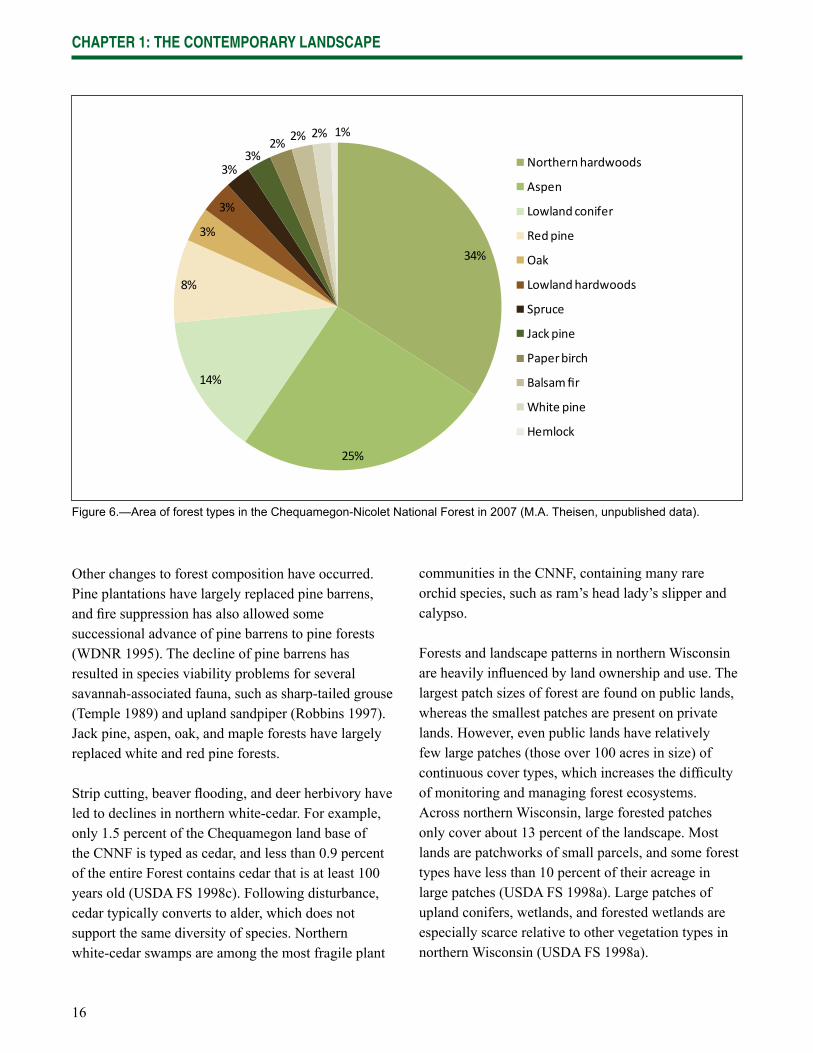
Forest Types on the Chequamegon-Nicolet National Forest—The CNNF is primarily forested (85 percent) but also includes open areas (9 percent upland and 4 percent lowland) and water features (2 percent). Of the forested acreage, northern hardwood and aspen forests cover nearly 60 percent of the land base followed by lowland conifer and red pine forest (Fig. 6). Lowland conifer forests cover 32 percent of forested land in the CNNF compared to only 11 percent on privately owned forest lands (P.E. Pingrey, unpublished data).
Changes in Forest Ecosystems
Profound changes to northern ecosystems occurred between the 1850s and the early 1930s. Logging of eastern white pine began as early as the 1830s and peaked at the end of the century. The amount and extent of slash left after logging fueled intense and catastrophic fi res across most of northern Wisconsin. By the 1930s nearly all of the primary forest had been harvested or burned (WDNR 2009a). Clearcutting, slash burning, and stream and river modifi cations during the logging era, combined with repeated cutting and the suppression of natural disturbances, may have resulted in long-term changes in the ecosystems of northern Wisconsin (USDA FS 1998b). While pioneer species represented little of the northern forest before European settlement, a single pioneer community, the aspen/birch forest-type group, currently occupies about 25 percent of the area (Miles 2010).
Although the average age of long-lived tree species continued to increase from 1983 to 1996, the area occupied by stands more than 100 years old continued to decrease from already low amounts (Schmidt 1997, Spencer et al. 1988). Frelich and Reich (1996) estimated that the current acreage (911,799 acres) of primary (unlogged) forest in 1996 in Minnesota, Wisconsin, and Michigan represented 1.1 percent of its 1850 abundance (80,769,511 ac).
15
CHAPTER 1: THE CONTEMPORARY LANDSCAPE
Forest-type group Percent cover Characteristic species (dominants and associates)
Maple/beech/birch 28 Sugar maple Basswood Quaking aspen (Acer saccharum) (Tilia americana) (Populus tremuloides) American beech White ash Yellow birch (Fagus grandifolia) (Fraxinus americana) (Betula alleghaniensis) Red maple Red oak (Acer rubrum) (Quercus rubra)
Aspen/birch 25 Quaking aspen Red maple (Populus tremuloides) (Acer rubrum) Big-tooth aspen Balsam fi r (Populus grandidentata) (Abies balsamea) Paper birch (Betula papyrifera)
Oak/hickory 13 Red oak Red maple Black oak (Quercus rubra) (Acer rubrum) (Quercus velutina) White oak Quaking aspen Bur oak (Quercus alba) (Populus tremuloides) (Quercus macrocarpa) Northern pin oak White pine Black cherry (Quercus ellipsoidalis) (Pinus strobus) (Prunus serotina)
Spruce/fi r 12 White spruce Northern white-cedar (Picea glauca) (Thuja occidentalis) Balsam fi r Tamarack (Abies balsamea) (Larix laricina) Black spruce (Picea mariana)
Elm/ash/cottonwood 9 Black ash American elm (Fraxinus nigra) (Ulmus americana) Green ash Silver maple (Fraxinus pennsylvanica) (Acer saccharinum) Red maple (Acer rubrum)
White/red/jack pine 8 White pine Red oak Quaking aspen (Pinus strobus) (Quercus rubra) (Populus tremuloides) Red pine Northern pin oak Big-tooth aspen (Pinus resinosa) (Quercus ellipsoidalis) (Populus grandidentata) Jack pine Red maple (Pinus banksiana) (Acer rubrum)
Oak/pine 3 Red oak White ash Sugar maple (Quercus rubra) (Fraxinus americana) (Acer saccharum) White pine Basswood (Pinus strobus) (Tilia americana) Red maple Big-tooth aspen (Acer rubrum) (Populus grandidentata)
Other 1 Includes mixed species stands not easily categorized and areas that cannot support forest cover because of rocks, water, and other impediments to stocking
Table 1.—Forest type groups of northern Wisconsin.
16
CHAPTER 1: THE CONTEMPORARY LANDSCAPE
34%
25%
14%
8%
3%
3%
3%3%
2% 2% 2% 1%
Northernhardwoods
Aspen
Lowland conifer
Redpine
Oak
Lowlandhardwoods
Spruce
Jack pine
Paperbirch
Balsamfir
White pine
Hemlock
Figure 6.—Area of forest types in the Chequamegon-Nicolet National Forest in 2007 (M.A. Theisen, unpublished data).
Other changes to forest composition have occurred. Pine plantations have largely replaced pine barrens, and fi re suppression has also allowed some successional advance of pine barrens to pine forests (WDNR 1995). The decline of pine barrens has resulted in species viability problems for several savannah-associated fauna, such as sharp-tailed grouse (Temple 1989) and upland sandpiper (Robbins 1997). Jack pine, aspen, oak, and maple forests have largely replaced white and red pine forests.
Strip cutting, beaver fl ooding, and deer herbivory have led to declines in northern white-cedar. For example, only 1.5 percent of the Chequamegon land base of the CNNF is typed as cedar, and less than 0.9 percent of the entire Forest contains cedar that is at least 100 years old (USDA FS 1998c). Following disturbance, cedar typically converts to alder, which does not support the same diversity of species. Northern white-cedar swamps are among the most fragile plant
communities in the CNNF, containing many rare orchid species, such as ram’s head lady’s slipper and calypso.
Forests and landscape patterns in northern Wisconsin are heavily infl uenced by land ownership and use. The largest patch sizes of forest are found on public lands, whereas the smallest patches are present on private lands. However, even public lands have relatively few large patches (those over 100 acres in size) of continuous cover types, which increases the diffi culty of monitoring and managing forest ecosystems. Across northern Wisconsin, large forested patches only cover about 13 percent of the landscape. Most lands are patchworks of small parcels, and some forest types have less than 10 percent of their acreage in large patches (USDA FS 1998a). Large patches of upland conifers, wetlands, and forested wetlands are especially scarce relative to other vegetation types in northern Wisconsin (USDA FS 1998a).
17
CHAPTER 1: THE CONTEMPORARY LANDSCAPE
Natural disturbance regimes—Severe wind and fi re events are the primary natural disturbances responsible for the vegetation patterning in northern Wisconsin. Before European settlement, wind events such as gales, derechos, and tornadoes occurred in all forest types and were more frequent and affected more area than fi res (Schulte and Mladenoff 2005). Fire events were more likely to occur in fi re-dependant forest types, such as jack, red, and white pine forests. The role of fi re in the natural disturbance regime of mesic upland hardwood forests was minimal. The return intervals of stand-replacing fi res are approximately 6,500 years for sugar maple-basswood forests and 14,300 years for yellow birch-hardwood forests (Schulte and Mladenoff 2005). Fire-return intervals are about 10 times longer today than they were in pre-settlement times (Cleland et al. 2008).
Windthrow events vary in extent and in the degree of tree mortality that they cause, in part, because of differences in susceptibility among species and age classes (Rich et al. 2007). Return intervals for windthrow events such as derechos vary geographically and have not been consistent over the past 40 years (Coniglio and Stensrud 2004).
Pests and diseases—Insect and disease outbreaks have also infl uenced the vegetation structure of northern Wisconsin (WDNR 2007). Before European settlement, outbreaks were caused by native species. For example, outbreaks of jack pine budworm and spruce budworm have been an important agent of mortality for their host species. Historically, wildfi res commonly occurred in areas of high mortality following such outbreaks. More recently, insect and disease outbreaks have occurred at an increasing frequency as a consequence of the increasing rate of introduction and establishment of nonnative insects and disease agents. Emerald ash borer, a beetle that can cause near complete mortality of ash tree populations throughout the eastern United States,
has been confi rmed in several Wisconsin locations. Outbreaks of the nonnative gypsy moth have caused oak mortality and fungal diseases such as oak wilt and butternut canker, resulting in tree mortality on smaller scales. European earthworms are discussed less often, but may have wide-ranging and profound effects on northern forests, which have not experienced earthworm activity for millennia (Bohlen et al. 2004). Climatic changes, such as prolonged heat and drought stress, can lead to increases in incidence or severity of insect and disease outbreaks, although it may also slow the spread of pests such as earthworms.
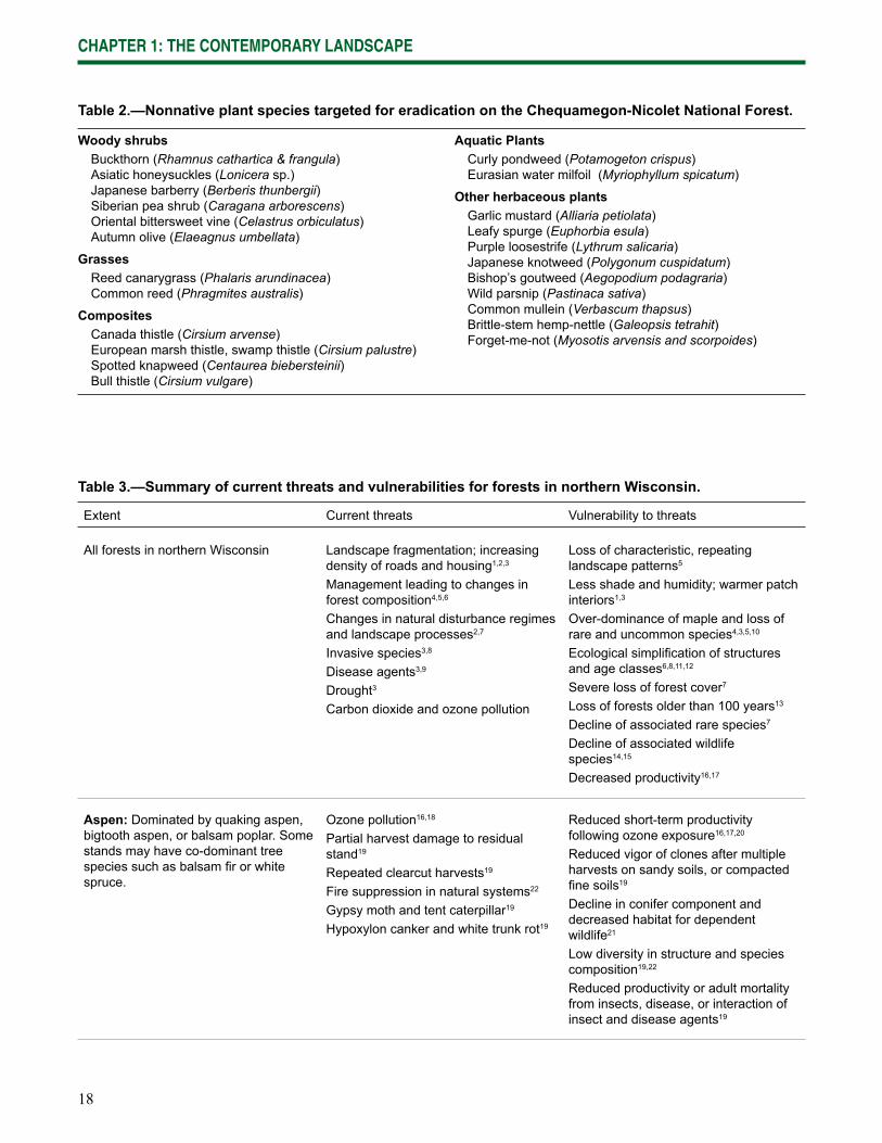
Invasive plant species—Nonnative plant species have become an increasing concern across northern Wisconsin because of their potential to outcompete native species and impact species interactions that are important to ecosystem function. Some nonnatives can establish more rapidly than native species, in part, because native diseases or pests are not adapted to compete against them (Tu et al. 2001). The Wisconsin Department of Natural Resources recently completed a statewide classifi cation of invasive species in Wisconsin (WDNR 2009c), and in northern Wisconsin, several cooperative weed management areas have been established to control invasive plant species across political boundaries. The CNNF, like other land managers in northern Wisconsin, is actively combating the spread of nonnative, invasive plants with integrated pest management tools that include prescribed fi re, mechanical treatments, and herbicide application (Table 2).
Current vulnerabilities—The current forest ecosystems of northern Wisconsin continue to be exposed to a wide range of natural and human-caused threats. Individual threats or interactions among threats increase the vulnerability of these systems to declines in productivity or abundance (Table 3), many of which are likely to be exacerbated by climate change.
18
CHAPTER 1: THE CONTEMPORARY LANDSCAPE
Table 2.—Nonnative plant species targeted for eradication on the Chequamegon-Nicolet National Forest.
Woody shrubs Buckthorn (Rhamnus cathartica & frangula) Asiatic honeysuckles (Lonicera sp.) Japanese barberry (Berberis thunbergii) Siberian pea shrub (Caragana arborescens) Oriental bittersweet vine (Celastrus orbiculatus) Autumn olive (Elaeagnus umbellata)
Grasses Reed canarygrass (Phalaris arundinacea) Common reed (Phragmites australis)
Composites Canada thistle (Cirsium arvense) European marsh thistle, swamp thistle (Cirsium palustre) Spotted knapweed (Centaurea biebersteinii) Bull thistle (Cirsium vulgare)
Aquatic Plants Curly pondweed (Potamogeton crispus) Eurasian water milfoil (Myriophyllum spicatum)
Other herbaceous plants Garlic mustard (Alliaria petiolata) Leafy spurge (Euphorbia esula) Purple loosestrife (Lythrum salicaria) Japanese knotweed (Polygonum cuspidatum) Bishop’s goutweed (Aegopodium podagraria) Wild parsnip (Pastinaca sativa) Common mullein (Verbascum thapsus) Brittle-stem hemp-nettle (Galeopsis tetrahit) Forget-me-not (Myosotis arvensis and scorpoides)
Extent Current threats Vulnerability to threats
All forests in northern Wisconsin Landscape fragmentation; increasing density of roads and housing1,2,3
Management leading to changes in forest composition4,5,6
Changes in natural disturbance regimes and landscape processes2,7
Invasive species3,8
Disease agents3,9
Drought3
Carbon dioxide and ozone pollution
Loss of characteristic, repeating landscape patterns5
Less shade and humidity; warmer patch interiors1,3
Over-dominance of maple and loss of rare and uncommon species4,3,5,10
Ecological simplifi cation of structures and age classes6,8,11,12
Severe loss of forest cover7
Loss of forests older than 100 years13 Decline of associated rare species7
Decline of associated wildlife species14,15
Decreased productivity16,17
Aspen: Dominated by quaking aspen, bigtooth aspen, or balsam poplar. Some stands may have co-dominant tree species such as balsam fi r or white spruce.
Ozone pollution16,18
Partial harvest damage to residual stand19
Repeated clearcut harvests19
Fire suppression in natural systems22
Gypsy moth and tent caterpillar19
Hypoxylon canker and white trunk rot19
Reduced short-term productivity following ozone exposure16,17,20
Reduced vigor of clones after multiple harvests on sandy soils, or compacted fi ne soils19
Decline in conifer component and decreased habitat for dependent wildlife21
Low diversity in structure and species composition19,22
Reduced productivity or adult mortality from insects, disease, or interaction of insect and disease agents19
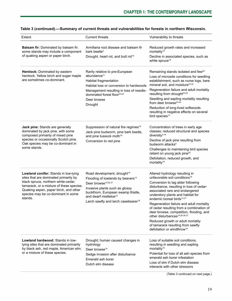
Table 3.—Summary of current threats and vulnerabilities for forests in northern Wisconsin.
19
CHAPTER 1: THE CONTEMPORARY LANDSCAPE
Table 3 (continued).—Summary of current threats and vulnerabilities for forests in northern Wisconsin.
Extent Current threats Vulnerability to threats
Balsam fi r: Dominated by balsam fi r; some stands may include a component of quaking aspen or paper birch.
Armillaria root disease and balsam fi r bark beetle3
Drought, heart rot, and butt rot19
Reduced growth rates and increased mortality19
Decline in associated species, such as white spruce19
Hemlock: Dominated by eastern hemlock. Yellow birch and sugar maple are sometimes co-dominant.
Rarity relative to pre-European abundance11
Habitat fragmentationHabitat loss or conversion to hardwoodsManagement resulting in loss of needle-dominated forest fl oor23,24
Deer browseDrought
Remaining stands isolated and few24
Loss of microsite conditions for seedling establishment, such as nurse logs, bare mineral soil, and moisture23,24
Regeneration failure and adult mortality resulting from drought23,24
Seedling and sapling mortality resulting from deer browse23,24
Reduction of long-lived softwoods resulting in negative effects on several bird species13
Jack pine: Stands are generally dominated by jack pine, with some composed primarily of mixed pine species or occasionally Scotch pine. Oak species may be co-dominant in some stands.
Suppression of natural fi re regimes19
Jack pine budworm, pine bark beetle, and pine tussock moth19
Conversion to red pine
Concentration of trees in early age classes; reduced structural and species diversity3,19
Decline of jack pine resulting from budworm attacks5
Challenges to maintaining bird species reliant on young jack pine25 Defoliation, reduced growth, and mortality19
Lowland conifer: Stands in low-lying sites that are dominated primarily by black spruce, northern white-cedar, tamarack, or a mixture of these species. Quaking aspen, paper birch, and other species may be co-dominant in some stands.
Road development; drought19
Flooding of lowlands by beavers13
Deer browse19,26,37
Invasive plants such as glossy buckthorn, European swamp thistle, and dwarf mistletoe19
Larch sawfl y and larch casebearer19
Altered hydrology resulting in unfavorable soil conditions19
Conversion to tag alder following disturbance, resulting in loss of cedar-associated rare and endangered understory plants and habitat for endemic boreal birds13,27
Regeneration failure and adult mortality of cedar resulting from a combination of deer browse, competition, fl ooding, and other disturbances19,26,28,37
Reduced growth or adult mortality of tamarack resulting from sawfl y defoliation or windthrow19
Lowland hardwood: Stands in low-lying sites that are dominated primarily by black ash, red maple, American elm, or a mixture of these species.
Drought; human caused changes in hydrologyDeer browse19
Sedge invasion after disturbanceEmerald ash borerDutch elm disease
Loss of suitable soil conditions, resulting in seedling and sapling mortality19
Potential for loss of all ash species from emerald ash borer infestationLoss of elm if Dutch elm disease interacts with other stressors
(Table 3 continued on next page.)
20
CHAPTER 1: THE CONTEMPORARY LANDSCAPE
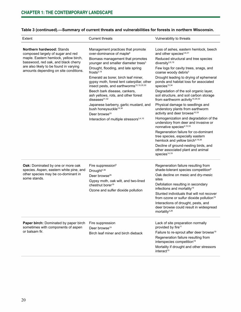
Northern hardwood: Stands composed largely of sugar and red maple. Eastern hemlock, yellow birch, basswood, red oak, and black cherry are also likely to be found in varying amounts depending on site conditions.
Management practices that promote over-dominance of maple6
Biomass management that promotes younger and smaller diameter trees3
Drought, fl ooding, and late spring frosts3,19
Emerald as borer, birch leaf miner, gypsy moth, forest tent caterpillar, other insect pests, and earthworms10,19,29,30
Beech bark disease, cankers, ash yellows, rots, and other forest diseases31,32
Japanese barberry, garlic mustard, and bush honeysuckle19,38
Deer browse33
Interaction of multiple stressors3,4,10
Loss of ashes, eastern hemlock, beech and other species3,6,31
Reduced structural and tree species diversity3,6,19
Few logs for cavity trees, snags, and coarse woody debris3
Drought leading to drying of ephemeral ponds and habitat loss for associated species15,34
Degradation of the soil organic layer, soil structure, and soil carbon storage from earthworm activity10,29,35
Physical damage to seedlings and understory plants from earthworm activity and deer browse10,33
Homogenization and degradation of the understory from deer and invasive or nonnative species4,10,33
Regeneration failure for co-dominant tree species, especially eastern hemlock and yellow birch4,19,26 Decline of ground-nesting birds, and other associated plant and animal species14,19
Oak: Dominated by one or more oak species. Aspen, eastern white pine, and other species may be co-dominant in some stands.
Fire suppression8
Drought3,36
Deer browse26
Gypsy moth, oak wilt, and two-lined chestnut borer19
Ozone and sulfer dioxide pollution
Regeneration failure resulting from shade-tolerant species competition8
Oak decline on mesic and dry-mesic sitesDefoliation resulting in secondary infections and mortality19
Stunted individuals that will not recover from ozone or sulfur dioxide pollution19
Interactions of drought, pests, and deer browse could result in widespread mortality3,26
Paper birch: Dominated by paper birch sometimes with components of aspen or balsam fi r.
Fire suppressionDeer browse19
Birch leaf miner and birch dieback
Lack of site preparation normally provided by fi re11
Failure to re-sprout after deer browse19
Regeneration failure resulting from interspecies competition19
Mortality if drought and other stressors interact19
Table 3 (continued).—Summary of current threats and vulnerabilities for forests in northern Wisconsin.
Extent Current threats Vulnerability to threats
21
CHAPTER 1: THE CONTEMPORARY LANDSCAPE
1Gonzalez-Abraham et al. 2007, 2Radeloff et al. 2005, 3WDNR 2010a, 4Powers and Nagel 2009, 5Radeloff et al. 1999, 6Crow et al. 2002, 7Canham and Loucks 1984, 8Nowacki et al. 1990, 9Schwingle 2010, 10Bohlen et al. 2004, 11Schulte et al. 2007, 12Rooney et al. 2004, 13USDA FS 2000, 14Martin et al. 2009, 15WDNR 1995, 16Pregitzer et al. 2008, 17Karnosky et al. 2003a, 18Karnosky et al. 2003b, 19WDNR 2010c, 20Karnosky et al. 2005, 21Zollner et al. 2008, 22Cleland et al.2001, 23Rooney et al. 2000, 24Mladenoff & Stearns 1993, 25Donner et al. 2009, 26Alverson et al. 1988, 27USDA FS 1998c, 28Heitzman et al. 1999, 29Hale et al. 2008, 30DATCP 2010, 31WDNR 2010b, 32WCF 2009, 33Rooney and Waller 2003, 34WDNR 2005, 35Gundale 2002, 36Rogers et al. 2008, 37Rooney et al. 2002, 38WDNR 2004.
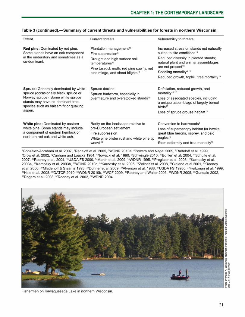
Table 3 (continued).—Summary of current threats and vulnerabilities for forests in northern Wisconsin.
Extent Current threats Vulnerability to threats
Red pine: Dominated by red pine. Some stands have an oak component in the understory and sometimes as a co-dominant.
Plantation management13
Fire suppression5
Drought and high surface soil temperatures19
Pine tussock moth, red pine sawfl y, red pine midge, and shoot blights19
Increased stress on stands not naturally suited to site conditions13
Reduced diversity in planted stands; natural plant and animal assemblages are not present13
Seedling mortality5,19
Reduced growth, topkill, tree mortality19
Spruce: Generally dominated by white spruce (occasionally black spruce or Norway spruce). Some white spruce stands may have co-dominant tree species such as balsam fi r or quaking aspen.
Spruce declineSpruce budworm, especially in overmature and overstocked stands19
Defoliation, reduced growth, and mortality19,27
Loss of associated species, including a unique assemblage of largely boreal birds13
Loss of spruce grouse habitat15
White pine: Dominated by eastern white pine. Some stands may include a component of eastern hemlock or northern red oak and white ash.
Rarity on the landscape relative to pre-European settlementFire suppressionWhite pine blister rust and white pine tip weevil19
Conversion to hardwoods5
Loss of supercanopy habitat for hawks, great blue herons, osprey, and bald eagles19
Stem deformity and tree mortality19
Fishermen on Kawaguesaga Lake in northern Wisconsin.
Pho
to b
y M
aria
K. J
anow
iak,
Nor
ther
n In
stitu
te o
f App
lied
Clim
ate
Sci
ence
an
d U
.S. F
ores
t Ser
vice
22
CHAPTER 1: THE CONTEMPORARY LANDSCAPE
Wildlife
Northern Wisconsin is home to hundreds of native animal species including more than 50 mammal species and approximately 250 bird species. A handful of mammal species have been extirpated from the state, including woodland caribou, bison, and wolverine. Others were lost but have been reintroduced, including the gray wolf, elk, and American marten. The gray wolf population in Wisconsin has grown from approximately 25 in 1980 to approximately 650 in the winter of 2008-2009 (Wydeven et al. 2009), with the majority of packs in located in the northern forests. A reintroduction of 25 elk in 1995 into the Clam Lake area (Ashland County) has not experienced the same level of success; there were approximately 130 in the summer of 2009 (Stowell and McKay 2009). Vehicle collisions, accidental shooting by hunters, and predation by wolves are leading mortality factors for elk.
Fishers, one of the largest members of the weasel family, were extirpated from northern Wisconsin in the early 1900s following widespread logging but successfully reintroduced in the 1950s and 1960s with rapid expansion of the population in the 1980s (Kohn et al. 1993). Trapping of fi sher in Wisconsin began in 1985 and continues today. American marten, likewise, were extirpated from northern Wisconsin following the logging era but reintroduction efforts have not been as successful. The species remains protected from trapping in Wisconsin despite population sizes suffi cient to allow harvesting in neighboring Minnesota and Michigan (Williams et al. 2007).
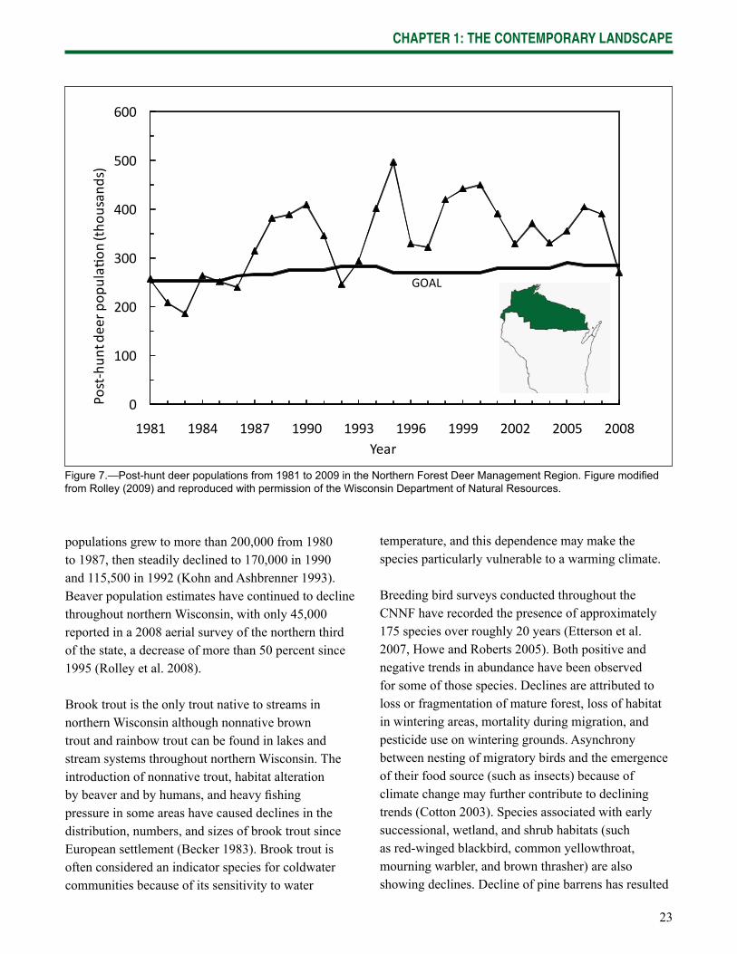
White-tailed deer are perhaps the wildlife species most identifi ed with northern Wisconsin. Deer hunting is a strong tradition throughout the state (Willging 2008) and many hunters travel to northern Wisconsin each autumn. The 2008 post-hunt white-tailed deer population in the Northern Forest region of Wisconsin was estimated at 270,000 animals, the lowest it has been in 15 years (Rolley 2009; Fig. 7). The long-term goal is to maintain a population of 270,000 animals,
which is 70 percent of the carrying capacity (WDNR 1998b). Deer have been called a keystone species due to their profound effect on forest structure and composition through their browsing patterns (Côté et al. 2004, Waller and Alverson 1997). Chronically high deer populations can suppress the regeneration of some tree species and can result in lower diversity of the whole forest community (Rooney and Waller 2003, Waller 2007).
Bald eagles favor super-canopy eastern white pines in the vicinity of fi sh-laden rivers and lakes for nesting sites. The bald eagle population in northern Wisconsin, and throughout the state, has steadily increased since the late 1960s following the ban on DDT. Statewide, the bald eagle population has increased from 108 active nests in 1973 to 1,142 nests in 2008 (Eckstein et al. 2008). Nearly 900 of those nests are present in the northern counties of Wisconsin.
Ruffed grouse are a common resident bird throughout all but the southeastern corner of Wisconsin (Robbins 1991). Ruffed grouse occurred statewide at the time of European settlement and were thought to be common in most areas, but relatively less common in the virgin conifer-hardwood forests of the north (Schorger 1945). After the logging era, regenerating forests in central and northern Wisconsin provided high quality grouse habitat (Schorger 1945). The relationship between aspen acreage, particularly 7 to 25 year old aspen, and grouse numbers (McCaffery et al. 1997) suggests that decreasing grouse populations may be the result of declines in aspen acreage (Perry et al. 2008).
Beaver, which were found throughout Wisconsin before 1800, were trapped heavily during European settlement and their statewide population had been reduced to 500 by 1900. Restricted trapping and favorable habitat changes resulted in a rapidly growing beaver population, and from 1940 to 1960 the population may have exceeded the historical level (Knudsen 1963). Beaver populations in the early 1950s were estimated at 120,000 to 170,000 in northern Wisconsin, and 50,000 in southern Wisconsin. Beaver
23
CHAPTER 1: THE CONTEMPORARY LANDSCAPE
populations grew to more than 200,000 from 1980 to 1987, then steadily declined to 170,000 in 1990 and 115,500 in 1992 (Kohn and Ashbrenner 1993). Beaver population estimates have continued to decline throughout northern Wisconsin, with only 45,000 reported in a 2008 aerial survey of the northern third of the state, a decrease of more than 50 percent since 1995 (Rolley et al. 2008).
Brook trout is the only trout native to streams in northern Wisconsin although nonnative brown trout and rainbow trout can be found in lakes and stream systems throughout northern Wisconsin. The introduction of nonnative trout, habitat alteration by beaver and by humans, and heavy fi shing pressure in some areas have caused declines in the distribution, numbers, and sizes of brook trout since European settlement (Becker 1983). Brook trout is often considered an indicator species for coldwater communities because of its sensitivity to water
temperature, and this dependence may make the species particularly vulnerable to a warming climate.
Breeding bird surveys conducted throughout the CNNF have recorded the presence of approximately 175 species over roughly 20 years (Etterson et al. 2007, Howe and Roberts 2005). Both positive and negative trends in abundance have been observed for some of those species. Declines are attributed to loss or fragmentation of mature forest, loss of habitat in wintering areas, mortality during migration, and pesticide use on wintering grounds. Asynchrony between nesting of migratory birds and the emergence of their food source (such as insects) because of climate change may further contribute to declining trends (Cotton 2003). Species associated with early successional, wetland, and shrub habitats (such as red-winged blackbird, common yellowthroat, mourning warbler, and brown thrasher) are also showing declines. Decline of pine barrens has resulted
0
100
200
300
400
500
600
1981 1984 1987 1990 1993 1996 1999 2002 2005 2008
Post-hun
tdeerp
opula
on(tho
usan
ds)
Year
GOAL
Figure 7.—Post-hunt deer populations from 1981 to 2009 in the Northern Forest Deer Management Region. Figure modifi ed from Rolley (2009) and reproduced with permission of the Wisconsin Department of Natural Resources.
24
CHAPTER 1: THE CONTEMPORARY LANDSCAPE
in species viability problems for several savannah-associated fauna, such as sharp-tailed grouse (Temple 1989) and upland sandpiper (Robbins 1997). Jack pine, aspen, oak, and maple forests have largely replaced white and red pine forests. Decline in mixed coniferous-deciduous forest has resulted in declining populations of birds associated with long-lived conifers. Of the 42 conifer-dependent bird species inhabiting the northern forests, 31 are rare (Green 1995).
Rare Elements
The Wisconsin Natural Heritage Inventory Working List contains species known or suspected to be rare in the state (WNHI 2009). It includes species legally designated as “Endangered” or “Threatened” as well as species in the advisory “Special Concern” category.
Because of the convergence of three major biomes and the variability in landforms and climate, the state supports over 2,000 native vascular plants, about 680 vertebrate animals, and as many as 65,000 invertebrates (WNHI 2009). Most recently, the Kirtland’s warbler, a species that is listed as endangered by the Federal government, has been documented breeding in young jack pine forests in central and northern Wisconsin. Eighty-six species on the Chequamegon-Nicolet National Forest are on the Regional Forester Sensitive Species list (Appendix 2) as well as State lists of threatened and endangered species or species of special concern. An additional 13 at-risk species have a high potential for occurrence on the Forest.
Additionally, several communities in northern Wisconsin have Natural Heritage rankings of “vulnerable globally” or rarer, indicating fewer than 100 occurrences of these communities globally: boreal forest, northern dry forest, northern wet-mesic forest, and pine barrens. For example, pine barrens are ranked as an imperiled community in Wisconsin and are also imperiled globally. Several butterfl y species that depend on pine barrens for habitat are also rare, including the Federally endangered Karner blue
butterfl y. The State endangered northern blue butterfl y and its State endangered plant host, dwarf bilberry, occur on pine barren remnants on the Nicolet land base of the CNNF (USDA FS 1998a).
Forest Ownership and Management
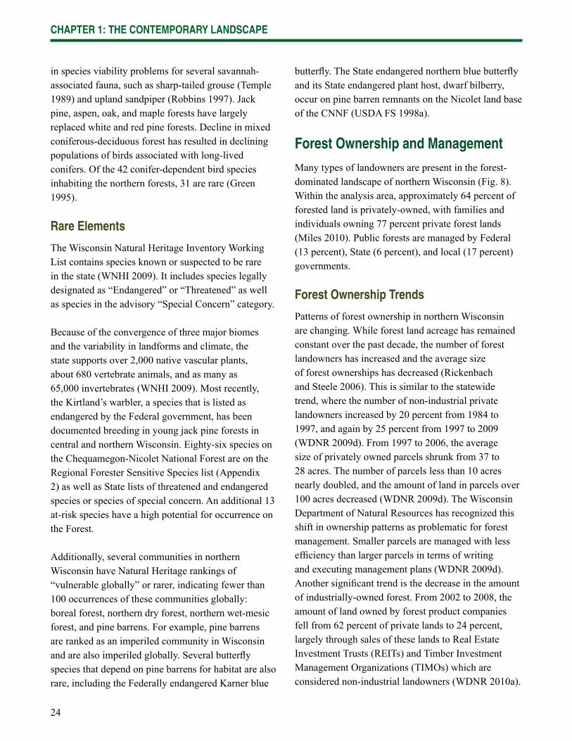
Many types of landowners are present in the forest-dominated landscape of northern Wisconsin (Fig. 8). Within the analysis area, approximately 64 percent of forested land is privately-owned, with families and individuals owning 77 percent private forest lands (Miles 2010). Public forests are managed by Federal (13 percent), State (6 percent), and local (17 percent) governments.
Forest Ownership Trends
Patterns of forest ownership in northern Wisconsin are changing. While forest land acreage has remained constant over the past decade, the number of forest landowners has increased and the average size of forest ownerships has decreased (Rickenbach and Steele 2006). This is similar to the statewide trend, where the number of non-industrial private landowners increased by 20 percent from 1984 to 1997, and again by 25 percent from 1997 to 2009 (WDNR 2009d). From 1997 to 2006, the average size of privately owned parcels shrunk from 37 to 28 acres. The number of parcels less than 10 acres nearly doubled, and the amount of land in parcels over 100 acres decreased (WDNR 2009d). The Wisconsin Department of Natural Resources has recognized this shift in ownership patterns as problematic for forest management. Smaller parcels are managed with less effi ciency than larger parcels in terms of writing and executing management plans (WDNR 2009d). Another signifi cant trend is the decrease in the amount of industrially-owned forest. From 2002 to 2008, the amount of land owned by forest product companies fell from 62 percent of private lands to 24 percent, largely through sales of these lands to Real Estate Investment Trusts (REITs) and Timber Investment Management Organizations (TIMOs) which are considered non-industrial landowners (WDNR 2010a).
25
CHAPTER 1: THE CONTEMPORARY LANDSCAPE
Some variations in forest composition in the region are refl ected in forest landownership. For example, public lands in the analysis area have higher proportions of aspen than lands under private ownership (Miles 2010), and the CNNF and State-owned forests have higher percentages of upland conifers (27 percent and 30 percent, respectively) than private lands (18 percent). However, overall differences in forest composition among forest ownerships are not substantial, suggesting that management among various landowners has been relatively similar (Miles 2010; Fig. 9).
Forest Management Programs for Private Landowners
Two programs provide tax relief to qualifi ed forest landowners. The Forest Crop Law program was enacted in 1927 as a means to promote private forestry. Enrollment closed in 1986, when the Managed Forest Law program was started, and the last participant contracts will expire in 2034 (WDOR 2009). Within
49%
17%
13%
10%
6%4%
1%
Individual
Local (county,municipal, etc.)
U.S. Forest Service
Corporate
State ofWisconsin
Na ve American (Indian)
Other
Figure 8.—Area of forest land by ownership in northern Wisconsin (Miles 2010).
the analysis area, 210,767 acres are enrolled in the Forest Crop Law program, which is approximately 80 percent of the total enrollment within the state (WDNR 2003, WDNR 2010a).
The Managed Forest Law, which has been revised a number of times, is designed to increase land retention and minimize fragmentation of parcels by reducing property taxes for participating forest landowners. Landowners with 10 acres or more may qualify, provided they incorporate broad ecosystem objectives into management and develop and implement comprehensive Forest Stewardship Plans. These plans qualify as Federal Forest Stewardship Plans and are a prerequisite for Federal cost-sharing assistance. Timber harvesting is permitted, offering owners a forest-based income stream that reduces pressure to generate revenue by other means, such as livestock grazing or development (P.E. Pingrey, personal communication). There were 2,124,698 acres in the analysis area participating in the MFL program in
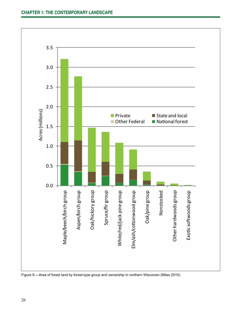
26
CHAPTER 1: THE CONTEMPORARY LANDSCAPE
Figure 9.—Area of forest land by forest-type group and ownership in northern Wisconsin (Miles 2010).
0.0
0.5
1.0
1.5
2.0
2.5
3.0
3.5
Maple/beech/birch
grou
p
Aspen/birch
grou
p
Oak/hickorygrou
p
Spruce/firgroup
White/red/jackpine
grou
p
Elm/ash/co
onwoo
dgrou
p
Oak/pinegrou
p
Non
stocked
Otherhardwoo
dsgrou
p
Exo
cso
woo
dsgrou
p
Private Stateand localOther Federal Na onal forest
Acres(m
illions)
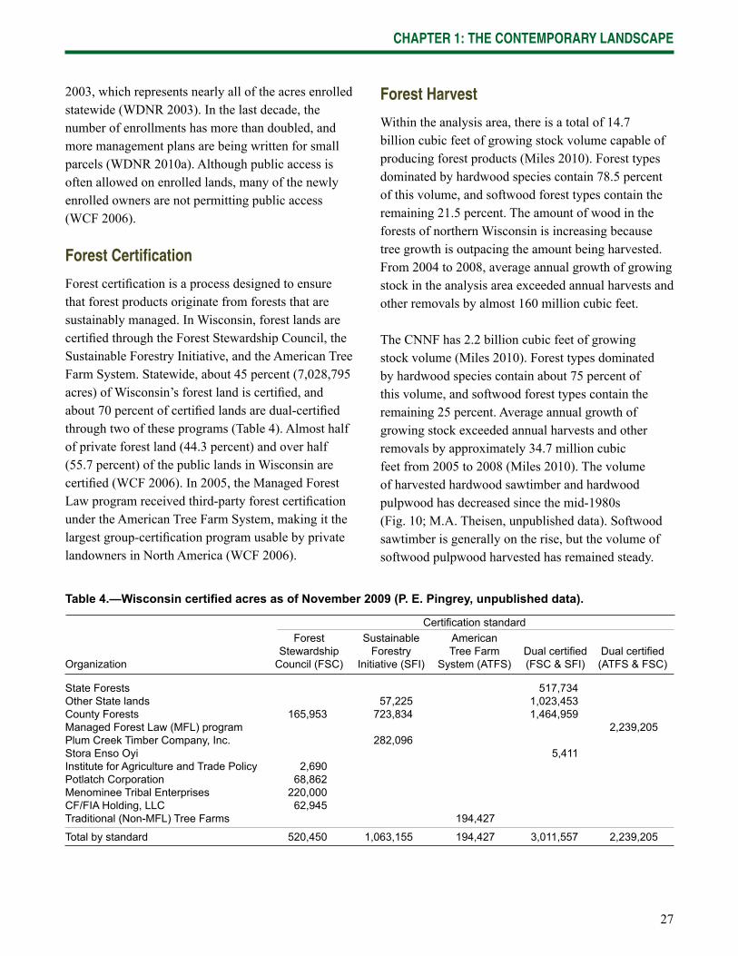
27
CHAPTER 1: THE CONTEMPORARY LANDSCAPE
2003, which represents nearly all of the acres enrolled statewide (WDNR 2003). In the last decade, the number of enrollments has more than doubled, and more management plans are being written for small parcels (WDNR 2010a). Although public access is often allowed on enrolled lands, many of the newly enrolled owners are not permitting public access (WCF 2006).
Forest Certifi cation
Forest certifi cation is a process designed to ensure that forest products originate from forests that are sustainably managed. In Wisconsin, forest lands are certifi ed through the Forest Stewardship Council, the Sustainable Forestry Initiative, and the American Tree Farm System. Statewide, about 45 percent (7,028,795 acres) of Wisconsin’s forest land is certifi ed, and about 70 percent of certifi ed lands are dual-certifi ed through two of these programs (Table 4). Almost half of private forest land (44.3 percent) and over half (55.7 percent) of the public lands in Wisconsin are certifi ed (WCF 2006). In 2005, the Managed Forest Law program received third-party forest certifi cation under the American Tree Farm System, making it the largest group-certifi cation program usable by private landowners in North America (WCF 2006).
Certifi cation standard Forest Sustainable American Stewardship Forestry Tree Farm Dual certifi ed Dual certifi edOrganization Council (FSC) Initiative (SFI) System (ATFS) (FSC & SFI) (ATFS & FSC)
State Forests 517,734 Other State lands 57,225 1,023,453 County Forests 165,953 723,834 1,464,959 Managed Forest Law (MFL) program 2,239,205Plum Creek Timber Company, Inc. 282,096 Stora Enso Oyi 5,411 Institute for Agriculture and Trade Policy 2,690 Potlatch Corporation 68,862 Menominee Tribal Enterprises 220,000 CF/FIA Holding, LLC 62,945 Traditional (Non-MFL) Tree Farms 194,427
Total by standard 520,450 1,063,155 194,427 3,011,557 2,239,205
Table 4.—Wisconsin certifi ed acres as of November 2009 (P. E. Pingrey, unpublished data).
Forest Harvest
Within the analysis area, there is a total of 14.7 billion cubic feet of growing stock volume capable of producing forest products (Miles 2010). Forest types dominated by hardwood species contain 78.5 percent of this volume, and softwood forest types contain the remaining 21.5 percent. The amount of wood in the forests of northern Wisconsin is increasing because tree growth is outpacing the amount being harvested. From 2004 to 2008, average annual growth of growing stock in the analysis area exceeded annual harvests and other removals by almost 160 million cubic feet.
The CNNF has 2.2 billion cubic feet of growing stock volume (Miles 2010). Forest types dominated by hardwood species contain about 75 percent of this volume, and softwood forest types contain the remaining 25 percent. Average annual growth of growing stock exceeded annual harvests and other removals by approximately 34.7 million cubic feet from 2005 to 2008 (Miles 2010). The volume of harvested hardwood sawtimber and hardwood pulpwood has decreased since the mid-1980s (Fig. 10; M.A. Theisen, unpublished data). Softwood sawtimber is generally on the rise, but the volume of softwood pulpwood harvested has remained steady.
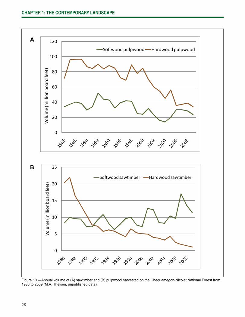
28
CHAPTER 1: THE CONTEMPORARY LANDSCAPE
Figure 10.—Annual volume of (A) sawtimber and (B) pulpwood harvested on the Chequamegon-Nicolet National Forest from 1986 to 2009 (M.A. Theisen, unpublished data).
A
B
0
20
40
60
80
100
120Vo
lume(m
illionbo
ardfeet)
So woodpulpwood Hardwoodpulpwood
0
5
10
15
20
25
Volume(m
illionbo
ardfeet)
So wood saw mber Hardwood saw mber
29
CHAPTER 1: THE CONTEMPORARY LANDSCAPE
In 2009, harvested sawtimber was 90 percent softwoods (11.3 million board feet) and 10 percent hardwoods (1.0 million board feet). Pulpwood harvested in 2009 was 60 percent hardwoods (34.0 million board feet) and 40 percent softwoods (23.6 million board feet; M.A. Theisen, unpublished data).
Socioeconomic Conditions
Approximately 5.7 million people lived in Wisconsin in 2009 (WDOA 2009a), about 1.5 million (27 percent) of whom resided in the 33 northern counties (WDOA 2009a). The population in northern Wisconsin increased 0.5 percent from 2008 to 2009, and 6.9 percent since 2000, which is slightly higher than the statewide rate. As the region becomes a more popular retirement destination, the median population age in northern Wisconsin is increasing (WDNR 2006).
According to the 2000 U.S. Census data for wage earners in northern Wisconsin counties, 28 percent earned less than $25,000 per year, 33 percent earned $25,000 to $49,000, and 22 percent earned $50,000 to $75,000. Only 16 percent had incomes greater than $75,000 per year in 2000 (USCB 2009). Thirty of the northern counties had poverty rates exceeding 10 percent from 2005 to 2007 (Isaacs and Smeeding 2009). The data from 2007 were the most recent county-level data available, but it is possible that poverty rates have risen with the recent increases in unemployment rates. The Wisconsin Department of Work Development estimated that unemployment rates in the northern counties have nearly doubled from 2008 (3.4 to 8.6 percent) to September of 2009 (6.7 to 17.7 percent). Unemployment rates during the previous year ranged from 3.4 to 8.6 percent (WDWD 2009).
The U.S. Census counted 386,234 families living in the northern counties in 2000, while the total estimated number of housing units was 688,291 (WDOA 2009b). Since 2000, the number of housing units has increased by an average of 1.3 percent per year (WDOA 2009b). Statewide, about 6 percent of housing units were used
for seasonal, recreational, or occasional purposes, compared to 14.3 percent in northern Wisconsin. In Bayfi eld, Burnett, Florence, Forest, and Sawyer counties, 40 to 50 percent of housing units were seasonal; Vilas County had more seasonal (56 percent) than primary units (WDOA 2009b).
Throughout Wisconsin, and particularly in northern Wisconsin, timber, recreation, and agriculture are signifi cant sectors of the economy.
Forest Products Industry
The forest products industry, much of which is supported by the heavily forested land base, is extremely important in northern Wisconsin. Although the total forest payroll and forest industry employment have been declining, forest industry in Wisconsin still generated 9 percent ($13.8 billion) of the total value of all manufacturing statewide and employed more than 68,000 people with wages totaling more than $3 billion per year (WDNR 2010a).
Paper and paperboard manufacturing consumes 52.8 percent of all roundwood (hardwood and softwood), which refl ects the regional importance of this industry. Of the $20.5 billion in wood products shipped in 2006, 67 percent came from the paper sector (WDNR 2010a). Further, despite recent mill closures, the paper sector still contributes 9 percent ($13.8 billion) of the total value of all manufacturing shipments statewide. Sawlogs are second, followed by composite products, fuelwood, veneer logs, and other products (WDNR 2010a).
Northern Wisconsin contains much of the infrastructure for the state’s forest industry. Of the state’s 273 sawmills, 171 are located in northern Wisconsin, as are all 13 veneer mills, the only excelsior mill, and most of the chip, pulp, and post-and-pole mills. However, only 40 percent of the particleboard mills are in northern Wisconsin (UWM 2006).
30
CHAPTER 1: THE CONTEMPORARY LANDSCAPE
Total wood product output for the state has declined in value since 2000, a peak year for the wood products industry (WDNR 2010a). Although the numbers for the most recent harvest years have not yet been analyzed, this trend is expected to continue as a result of the depressed global economy and competition from other wood-producing countries. New biomass technologies and markets, greenhouse gas legislation, and high oil barrel prices are expected to increase the value of wood products as the economy recovers (WDNR 2010a). In 2003, nearly 361 million cubic feet of products were produced from forests across Wisconsin (Perry et al. 2008). These products were primarily composed of pulpwood and composites (70 percent) and saw log products (27 percent; Perry et al. 2008). More softwood is being used as saw logs in 2007 and less in pulpwood, a trend attributed to the maturation of softwood stands, especially red pine plantations harvested at larger diameters (WDNR 2010a). Conversely, as hardwood saw log resources become less available, smaller diameter hardwood is making up a majority of the wood used for pulpwood and composite products (WDNR 2010a).
Recreation
Recreation is economically signifi cant throughout Wisconsin and is estimated to generate approximately $2.5 billion dollars a year through travel- and equipment-related revenue (WDNR 2010a). Recreation pressure on public lands is expected to increase as parcelization continues to decrease the amount of land open to the public (WDNR 2010a). Approximately 5.8 million acres of public land was available for recreation in 2006 (WDNR 2006).
Recreation and tourism are important to the overall economy of northern Wisconsin, which offers a range of experiences to its residents and visitors, from solitude and nature study to ATV (all-terrain vehicle) riding opportunities. Northern and rural counties are
dependent on resource-based tourism (Stynes 1997). Popular activities in northern Wisconsin include fi shing, camping, boating, golf, hunting, hiking, and bird watching. Many recreational opportunities are centered around water features (WDNR 2006).
Hunting remains popular in northern Wisconsin, but the number of hunters has been dropping as part of a 30-year national trend. In the past decade, participation in some recreational activities such as biking, cross-country skiing, and ATV riding has been increasing. ATV use, in particular, continues to grow rapidly in northern Wisconsin (WDNR 2006). Snowmobiling continues to be popular, but demand for this recreational activity is declining due to fewer people taking up the activity and low snow levels in the past decade (WDNR 2006).
Agriculture
Agriculture is an important industry with over 15 million acres of farmland throughout Wisconsin. In 2007, agriculture contributed about 9 percent ($20.2 billion) to Wisconsin’s total income. The majority of this comes from the agricultural processing sectors such as dairy, which contributed $26.5 billion of total industrial output in 2007 (Deller and Williams 2009). About 10 percent of the state’s workforce is employed in the agricultural sector.
In the analysis area, 20 percent of total land area is used for agriculture, with most of these lands concentrated in the southern part of the region (WDNR 1998a). Most of this acreage is dedicated to the production of hay and corn. Soybeans, wheat, oats, and barley are also common crops. Wisconsin is also the top producer of cranberries in the country, with 14,000 of the 17,700 acres of cranberry bogs located in the northern counties. (USDA NASS 2009, WDNR 1998a).
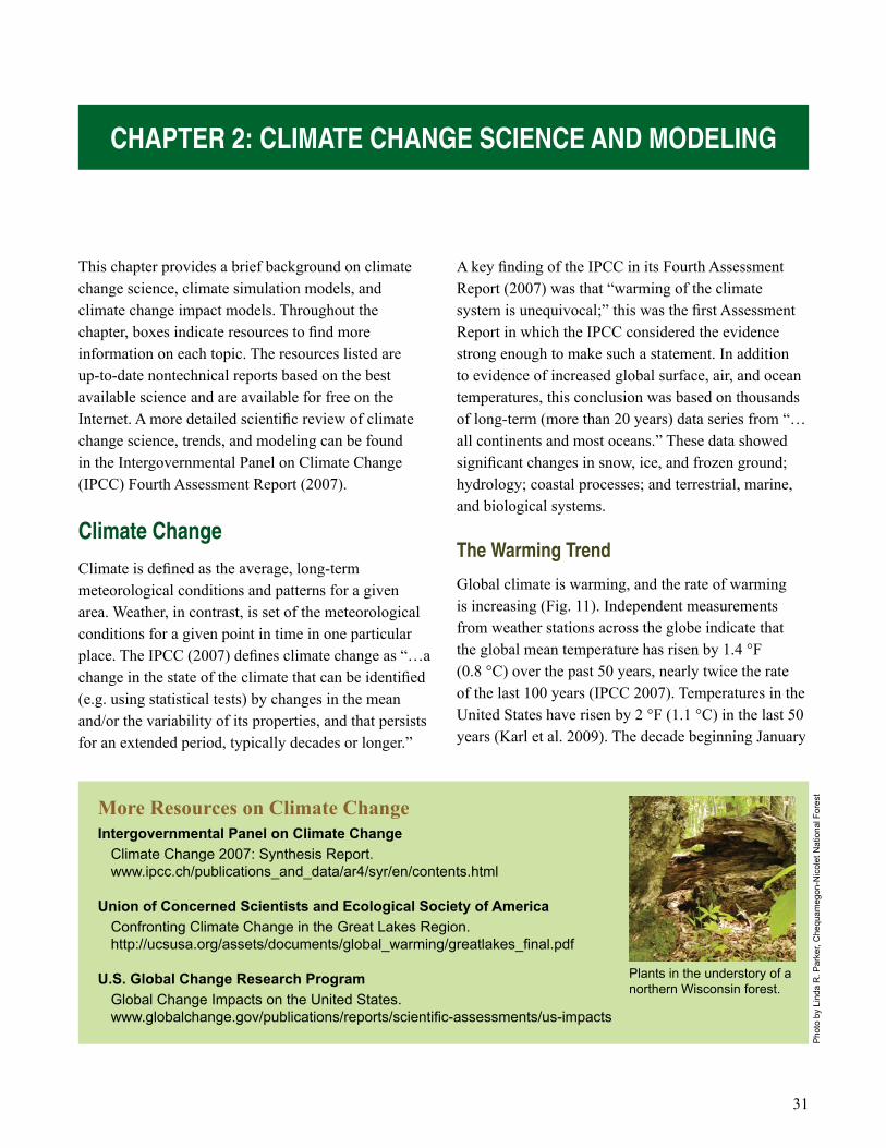
31
CHAPTER 2: CLIMATE CHANGE SCIENCE AND MODELING
This chapter provides a brief background on climate change science, climate simulation models, and climate change impact models. Throughout the chapter, boxes indicate resources to fi nd more information on each topic. The resources listed are up-to-date nontechnical reports based on the best available science and are available for free on the Internet. A more detailed scientifi c review of climate change science, trends, and modeling can be found in the Intergovernmental Panel on Climate Change (IPCC) Fourth Assessment Report (2007).
Climate Change
Climate is defi ned as the average, long-term meteorological conditions and patterns for a given area. Weather, in contrast, is set of the meteorological conditions for a given point in time in one particular place. The IPCC (2007) defi nes climate change as “…a change in the state of the climate that can be identifi ed (e.g. using statistical tests) by changes in the mean and/or the variability of its properties, and that persists for an extended period, typically decades or longer.”
A key fi nding of the IPCC in its Fourth Assessment Report (2007) was that “warming of the climate system is unequivocal;” this was the fi rst Assessment Report in which the IPCC considered the evidence strong enough to make such a statement. In addition to evidence of increased global surface, air, and ocean temperatures, this conclusion was based on thousands of long-term (more than 20 years) data series from “…all continents and most oceans.” These data showed signifi cant changes in snow, ice, and frozen ground; hydrology; coastal processes; and terrestrial, marine, and biological systems.
The Warming Trend
Global climate is warming, and the rate of warming is increasing (Fig. 11). Independent measurements from weather stations across the globe indicate that the global mean temperature has risen by 1.4 °F (0.8 °C) over the past 50 years, nearly twice the rate of the last 100 years (IPCC 2007). Temperatures in the United States have risen by 2 °F (1.1 °C) in the last 50 years (Karl et al. 2009). The decade beginning January
More Resources on Climate ChangeIntergovernmental Panel on Climate Change Climate Change 2007: Synthesis Report. www.ipcc.ch/publications_and_data/ar4/syr/en/contents.html
Union of Concerned Scientists and Ecological Society of America Confronting Climate Change in the Great Lakes Region. http://ucsusa.org/assets/documents/global_warming/greatlakes_fi nal.pdf
U.S. Global Change Research Program Global Change Impacts on the United States. www.globalchange.gov/publications/reports/scientifi c-assessments/us-impacts
Plants in the understory of a northern Wisconsin forest.
Pho
to b
y Li
nda
R. P
arke
r, C
hequ
ameg
on-N
icol
et N
atio
nal F
ores
t
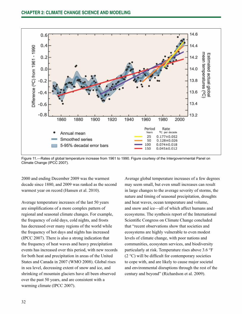
CHAPTER 2: CLIMATE CHANGE SCIENCE AND MODELING
32
2000 and ending December 2009 was the warmest decade since 1880, and 2009 was ranked as the second warmest year on record (Hansen et al. 2010).
Average temperature increases of the last 50 years are simplifi cations of a more complex pattern of regional and seasonal climate changes. For example, the frequency of cold days, cold nights, and frosts has decreased over many regions of the world while the frequency of hot days and nights has increased (IPCC 2007). There is also a strong indication that the frequency of heat waves and heavy precipitation events has increased over this period, with new records for both heat and precipitation in areas of the United States and Canada in 2007 (WMO 2008). Global rises in sea level, decreasing extent of snow and ice, and shrinking of mountain glaciers have all been observed over the past 50 years, and are consistent with a warming climate (IPCC 2007).
Figure 11.—Rates of global temperature increase from 1961 to 1990. Figure courtesy of the Intergovernmental Panel on Climate Change (IPCC 2007).
Average global temperature increases of a few degrees may seem small, but even small increases can result in large changes to the average severity of storms, the nature and timing of seasonal precipitation, droughts and heat waves, ocean temperature and volume, and snow and ice—all of which affect humans and ecosystems. The synthesis report of the International Scientifi c Congress on Climate Change concluded that “recent observations show that societies and ecosystems are highly vulnerable to even modest levels of climate change, with poor nations and communities, ecosystem services, and biodiversity particularly at risk. Temperature rises above 3.6 °F (2 °C) will be diffi cult for contemporary societies to cope with, and are likely to cause major societal and environmental disruptions through the rest of the century and beyond” (Richardson et al. 2009).

CHAPTER 2: CLIMATE CHANGE SCIENCE AND MODELING
33
Chapter 3 provides specifi c information about recent climate trends and future climate simulations for Wisconsin.
The Greenhouse Effect
The greenhouse effect is the process by which certain gases in the atmosphere absorb and re-emit energy that would otherwise be lost into space (Fig. 12). The greenhouse effect is necessary for human survival; without it Earth would have an average temperature of about 0 °F (-18 °C) and would be covered in ice.
Several naturally occurring greenhouse gases in the atmosphere contribute to the greenhouse effect,
including carbon dioxide, methane, nitrous oxide, and water vapor. Water vapor is the most abundant greenhouse gas, but is very responsive to driving factors such as temperature; its residence time in the atmosphere is on the order of days. Other greenhouse gases, including carbon dioxide, methane, and nitrous oxide, are likely to reside in the atmosphere for decades to centuries after initial introduction. Addition of these long-lived gases to the atmosphere will thus cause long-term warming. A warmer atmosphere is able to hold more water vapor, potentially leading to higher annual precipitation in some places, but also further increasing warming.
Figure 12.—An idealized model of the natural greenhouse effect. Figure courtesy of the Intergovernmental Panel on Climate Change (IPCC 2007).
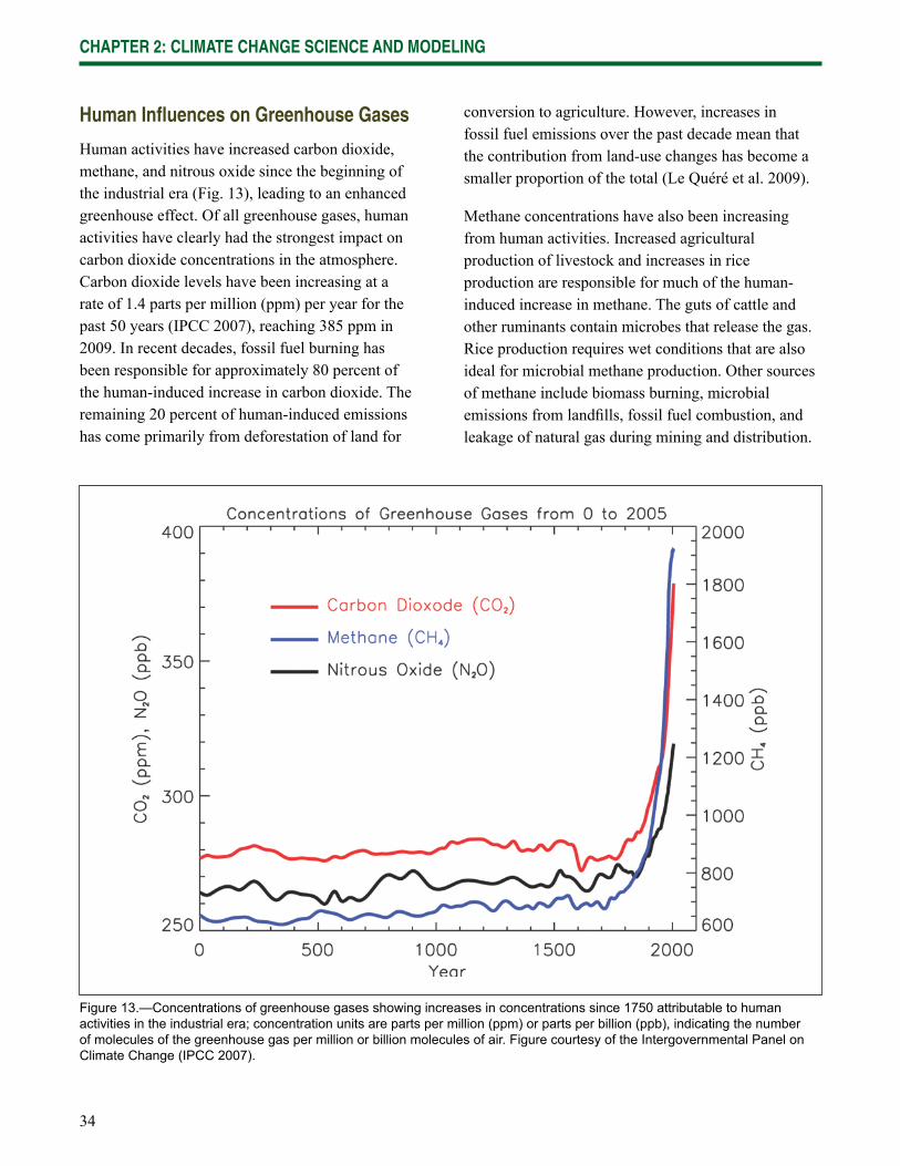
CHAPTER 2: CLIMATE CHANGE SCIENCE AND MODELING
34
Human Infl uences on Greenhouse Gases
Human activities have increased carbon dioxide, methane, and nitrous oxide since the beginning of the industrial era (Fig. 13), leading to an enhanced greenhouse effect. Of all greenhouse gases, human activities have clearly had the strongest impact on carbon dioxide concentrations in the atmosphere. Carbon dioxide levels have been increasing at a rate of 1.4 parts per million (ppm) per year for the past 50 years (IPCC 2007), reaching 385 ppm in 2009. In recent decades, fossil fuel burning has been responsible for approximately 80 percent of the human-induced increase in carbon dioxide. The remaining 20 percent of human-induced emissions has come primarily from deforestation of land for
conversion to agriculture. However, increases in fossil fuel emissions over the past decade mean that the contribution from land-use changes has become a smaller proportion of the total (Le Quéré et al. 2009).
Methane concentrations have also been increasing from human activities. Increased agricultural production of livestock and increases in rice production are responsible for much of the human-induced increase in methane. The guts of cattle and other ruminants contain microbes that release the gas. Rice production requires wet conditions that are also ideal for microbial methane production. Other sources of methane include biomass burning, microbial emissions from landfi lls, fossil fuel combustion, and leakage of natural gas during mining and distribution.
Figure 13.—Concentrations of greenhouse gases showing increases in concentrations since 1750 attributable to human activities in the industrial era; concentration units are parts per million (ppm) or parts per billion (ppb), indicating the number of molecules of the greenhouse gas per million or billion molecules of air. Figure courtesy of the Intergovernmental Panel on Climate Change (IPCC 2007).
CHAPTER 2: CLIMATE CHANGE SCIENCE AND MODELING
35
Sources of nitrous oxide are less well-understood than methane and carbon dioxide, but the consensus based on current science is that the primary human source of nitrous oxide is from agricultural activities. Increased fertilizer use on agricultural fi elds is responsible for increases in emissions from soil, which is released when soil microbes break down nitrogen-containing products. In addition to increased fertilizer use, the conversion of tropical forests to agricultural lands can lead to increases in microbial nitrous oxide production. Other sources of production include nylon production and combustion of fossil fuels.
Ozone, in addition to providing protection from the sun’s ultraviolet (UV) rays, is a naturally occurring greenhouse gas. Interception of harmful UV rays by ozone in the upper atmosphere, or stratosphere, is benefi cial to plants and animals. Human emissions of ozone-depleting substances such as chlorofl uorocarbons (CFCs) led to decreases in stratospheric ozone, which decreased both UV protection from the sun and ozone-induced warming. Regulation under the Montreal Protocol led to a decline in CFC emissions and reductions in ozone have subsequently slowed. Vehicle exhaust can lead to the production of tropospheric ozone, the ozone responsible for smog and increased local warming in urban areas.
Halocarbons, which include CFCs, are a class of chemical compounds that contain carbon and a halide such as fl uorine, chlorine, or bromine. After CFCs were banned, another class of halocarbons, hydrofl uorocarbons (HFCs, also known as “F-gases”), was used as a replacement for CFCs in refrigeration and air conditioning. HFCs do not deplete stratospheric ozone, but many are powerful greenhouse gases.
In addition to greenhouse gases, particulate matter in the atmosphere can also infl uence climate. These particles are known as aerosols, meaning suspensions of solids in the air (not to be confused with pressurized
sprays). Naturally occurring aerosols form from volcanic activity and forest fi res. Human additions to atmospheric aerosols come from vehicle exhaust, burning coal and other fossil fuels, and burning wood. Some of these particles refl ect radiation, while others absorb it, so changes in aerosol concentration can have a cooling effect or a warming effect. There is still some uncertainty about how aerosols will affect future climate, but the scientifi c consensus is that the effects will not outweigh the warming effects of greenhouse gases (Fig. 14).
Climate Models
Although we have estimated climate of the distant past using proxies and have measured climate directly in the recent past, we cannot “measure” future climate. Scientists instead use models to simulate future climate. These models are judged in part by their ability to accurately simulate past climate against proxy estimates. A model is a simplifi ed representation of reality. Models can be theoretical, mathematical, conceptual, or physical. The most important models used in climate science are general circulation models, which combine complex mathematical formulas representing physical processes in the ocean, atmosphere, and land surface within large computer simulations.
General Circulation Models
Mathematical models that simulate the general circulation of the atmosphere or oceans are called general circulation models (GCMs). GCMs simulate physical processes on the Earth’s surface, oceans, and atmosphere through time using mathematical equations in three-dimensional space. GCMs can work in time steps as small as minutes or hours in simulations covering decades to centuries. Because of their high level of complexity, GCMs require intensive computing power, and must be run on immense supercomputers.
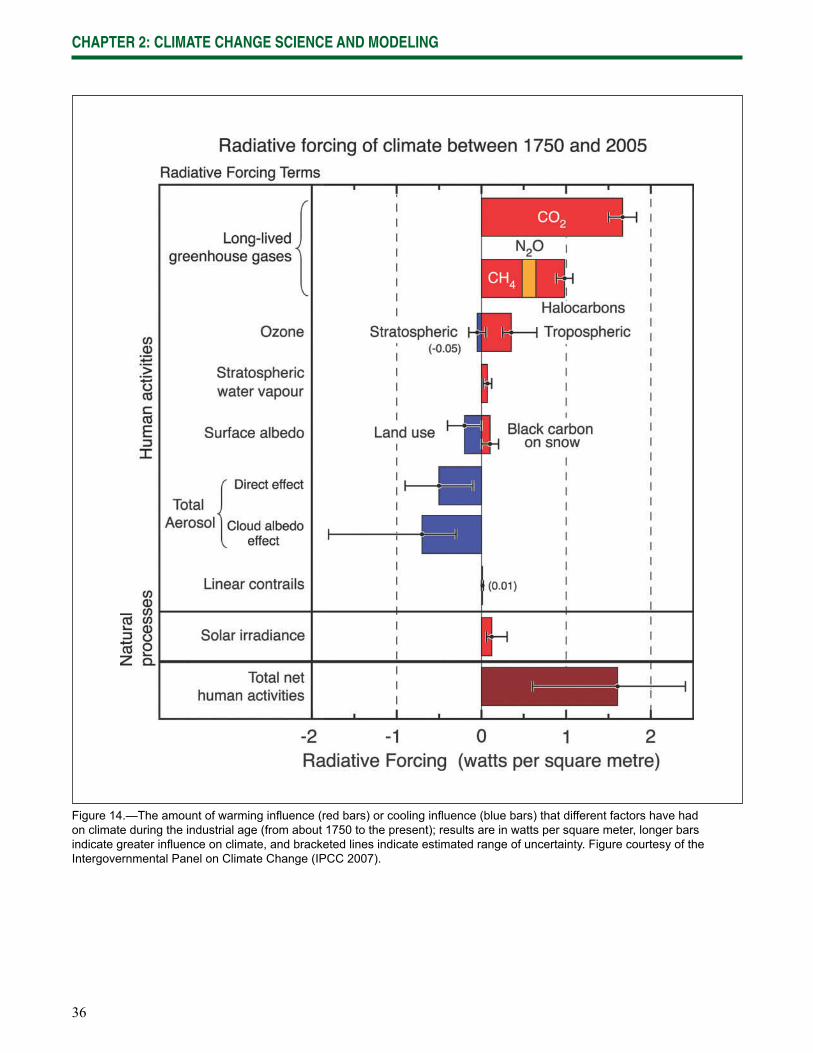
CHAPTER 2: CLIMATE CHANGE SCIENCE AND MODELING
36
Figure 14.—The amount of warming infl uence (red bars) or cooling infl uence (blue bars) that different factors have had on climate during the industrial age (from about 1750 to the present); results are in watts per square meter, longer bars indicate greater infl uence on climate, and bracketed lines indicate estimated range of uncertainty. Figure courtesy of the Intergovernmental Panel on Climate Change (IPCC 2007).
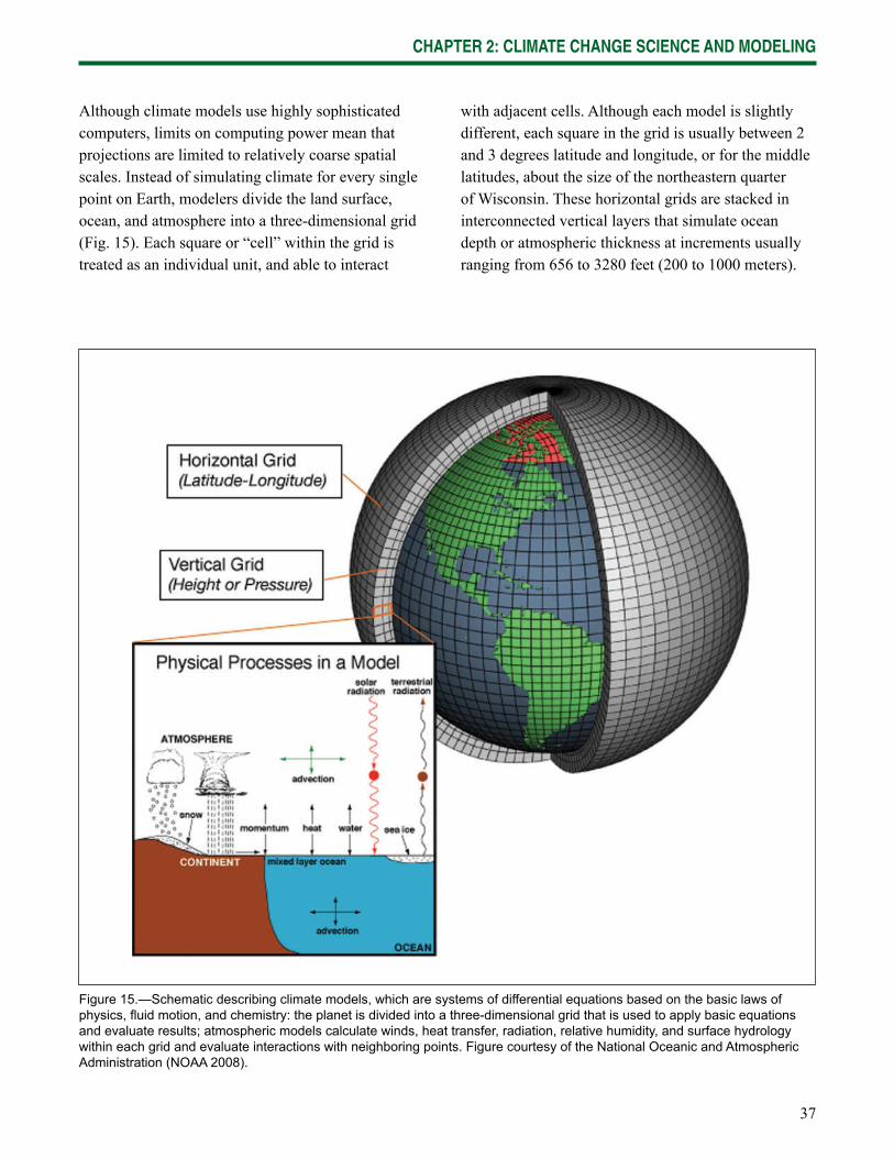
CHAPTER 2: CLIMATE CHANGE SCIENCE AND MODELING
37
Figure 15.—Schematic describing climate models, which are systems of differential equations based on the basic laws of physics, fl uid motion, and chemistry: the planet is divided into a three-dimensional grid that is used to apply basic equations and evaluate results; atmospheric models calculate winds, heat transfer, radiation, relative humidity, and surface hydrology within each grid and evaluate interactions with neighboring points. Figure courtesy of the National Oceanic and Atmospheric Administration (NOAA 2008).
Although climate models use highly sophisticated computers, limits on computing power mean that projections are limited to relatively coarse spatial scales. Instead of simulating climate for every single point on Earth, modelers divide the land surface, ocean, and atmosphere into a three-dimensional grid (Fig. 15). Each square or “cell” within the grid is treated as an individual unit, and able to interact
with adjacent cells. Although each model is slightly different, each square in the grid is usually between 2 and 3 degrees latitude and longitude, or for the middle latitudes, about the size of the northeastern quarter of Wisconsin. These horizontal grids are stacked in interconnected vertical layers that simulate ocean depth or atmospheric thickness at increments usually ranging from 656 to 3280 feet (200 to 1000 meters).
CHAPTER 2: CLIMATE CHANGE SCIENCE AND MODELING
38
Several research groups from around the world have developed GCMs that have been used in climate projections for the IPCC reports and elsewhere. GCMs have been developed by internationally renowned climate research centers such as NOAA’s Geophysical Fluid Dynamics Laboratory (GFDL CM2; Delworth et al. 2006), the UK’s Hadley Center (HadCM3; Pope 2000), and the National Center for Atmospheric Research (PCM; Washington et al. 2000), among others. These models use slightly different grid sizes and ways of quantitatively representing physical processes. They also differ in sensitivity to changes in greenhouse gas concentrations, which means that some models will tend to project higher increases in temperature than others under increasing greenhouse gas concentrations.
GCMs, like all models, have strengths and weaknesses. In general, they are useful and reliable tools because they are based on well-understood physical processes and have been successful at projecting climate and weather conditions. GCM simulations can also be run for past climate, and output from these simulations generally correspond well with proxy-based estimates of ancient climates and actual historical measurements of recent climates. GCM projections are not perfect, however. Sources of error in model output include incomplete scientifi c understanding of some climate processes, and the fact that some infl uential climate processes occur at spatial scales that are too small to be modeled with
current computing power. Technological advances in the computing industry along with scientifi c advances in our understanding of Earth’s physical processes will lead to continued improvements in GCM projections.
Emissions scenarios
Modelers must specify inputs into their GCM in order to perform a projection of future climatic conditions. Some of these inputs, like future greenhouse gas concentrations, are not known and must be estimated. Although human population growth, economic circumstances, and technological developments will certainly have dramatic effects on future greenhouse gas concentrations, they depend on social developments that cannot be completely foreseen. One common approach for dealing with uncertainty about future greenhouse gas concentrations is to develop alternative storylines about how the future may unfold and then calculate the potential greenhouse gas concentrations for each alternative storyline. The IPCC has established a set of standard emissions scenarios that represent a range of different storylines (IPCC 2007). When these scenarios are input into GCMs, differences in climate projections can be compared for each emissions scenario.
Emissions scenarios are a quantitative representation of alternative storylines given certain demographic, technological, or environmental developments. None of the current scenarios include any changes in
More Resources on Climate Models and Emissions ScenariosU.S. Global Change Research Program Climate Models: an Assessment of Strengths and Limitations. www.globalchange.gov/publications/reports/scientifi c-assessments/saps/sap3-1
Intergovernmental Panel on Climate Change Chapter 8: Climate Models and Their Evaluation www.ipcc.ch/publications_and_data/ar4/wg1/en/ch8.html Special Report on Emissions Scenarios: Summary for Policymakers. www.ipcc.ch/ipccreports/sres/emission/index.php?idp=0
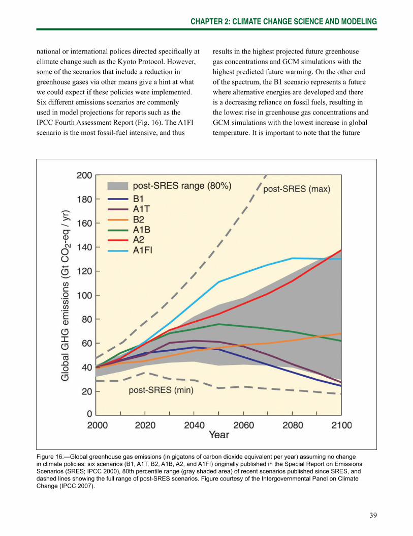
CHAPTER 2: CLIMATE CHANGE SCIENCE AND MODELING
39
Figure 16.—Global greenhouse gas emissions (in gigatons of carbon dioxide equivalent per year) assuming no change in climate policies: six scenarios (B1, A1T, B2, A1B, A2, and A1FI) originally published in the Special Report on Emissions Scenarios (SRES; IPCC 2000), 80th percentile range (gray shaded area) of recent scenarios published since SRES, and dashed lines showing the full range of post-SRES scenarios. Figure courtesy of the Intergovernmental Panel on Climate Change (IPCC 2007).
national or international polices directed specifi cally at climate change such as the Kyoto Protocol. However, some of the scenarios that include a reduction in greenhouse gases via other means give a hint at what we could expect if these policies were implemented. Six different emissions scenarios are commonly used in model projections for reports such as the IPCC Fourth Assessment Report (Fig. 16). The A1FI scenario is the most fossil-fuel intensive, and thus
results in the highest projected future greenhouse gas concentrations and GCM simulations with the highest predicted future warming. On the other end of the spectrum, the B1 scenario represents a future where alternative energies are developed and there is a decreasing reliance on fossil fuels, resulting in the lowest rise in greenhouse gas concentrations and GCM simulations with the lowest increase in global temperature. It is important to note that the future
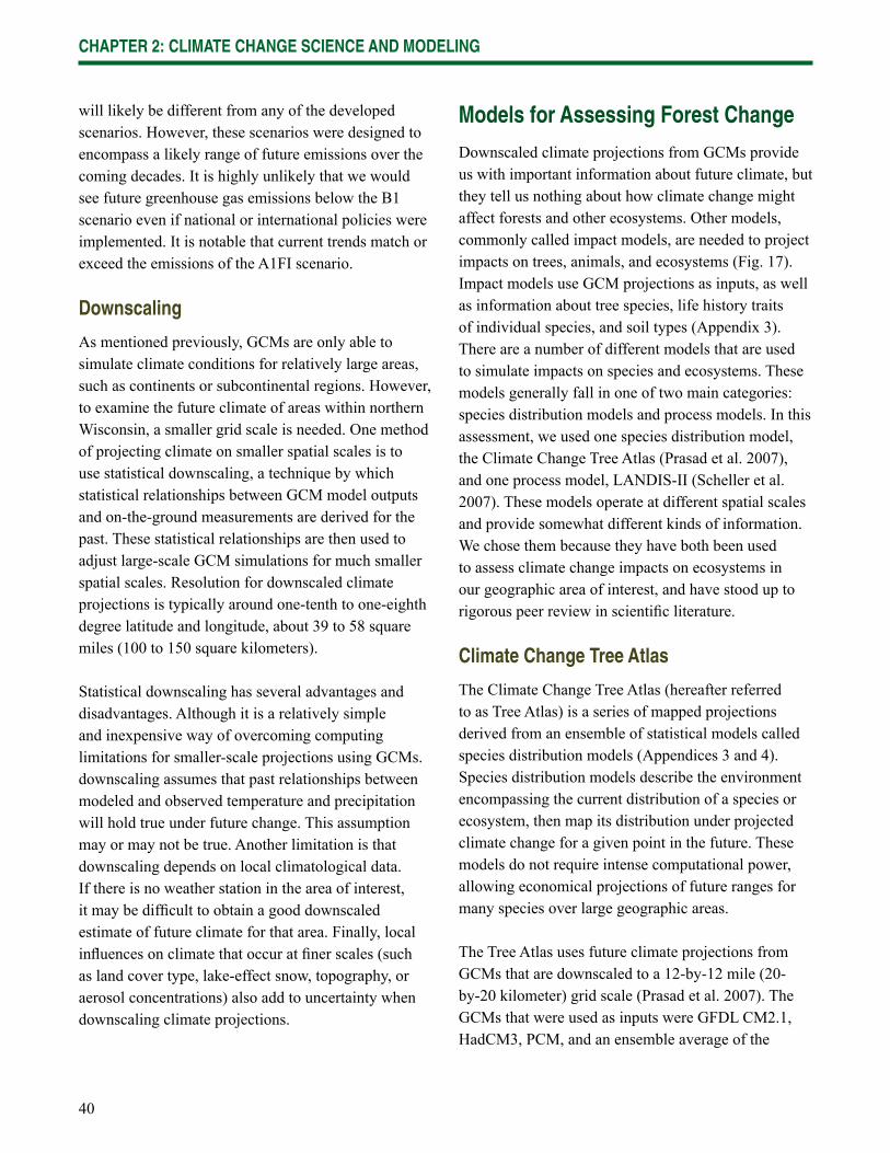
CHAPTER 2: CLIMATE CHANGE SCIENCE AND MODELING
40
will likely be different from any of the developed scenarios. However, these scenarios were designed to encompass a likely range of future emissions over the coming decades. It is highly unlikely that we would see future greenhouse gas emissions below the B1 scenario even if national or international policies were implemented. It is notable that current trends match or exceed the emissions of the A1FI scenario.
Downscaling
As mentioned previously, GCMs are only able to simulate climate conditions for relatively large areas, such as continents or subcontinental regions. However, to examine the future climate of areas within northern Wisconsin, a smaller grid scale is needed. One method of projecting climate on smaller spatial scales is to use statistical downscaling, a technique by which statistical relationships between GCM model outputs and on-the-ground measurements are derived for the past. These statistical relationships are then used to adjust large-scale GCM simulations for much smaller spatial scales. Resolution for downscaled climate projections is typically around one-tenth to one-eighth degree latitude and longitude, about 39 to 58 square miles (100 to 150 square kilometers).
Statistical downscaling has several advantages and disadvantages. Although it is a relatively simple and inexpensive way of overcoming computing limitations for smaller-scale projections using GCMs. downscaling assumes that past relationships between modeled and observed temperature and precipitation will hold true under future change. This assumption may or may not be true. Another limitation is that downscaling depends on local climatological data. If there is no weather station in the area of interest, it may be diffi cult to obtain a good downscaled estimate of future climate for that area. Finally, local infl uences on climate that occur at fi ner scales (such as land cover type, lake-effect snow, topography, or aerosol concentrations) also add to uncertainty when downscaling climate projections.
Models for Assessing Forest Change
Downscaled climate projections from GCMs provide us with important information about future climate, but they tell us nothing about how climate change might affect forests and other ecosystems. Other models, commonly called impact models, are needed to project impacts on trees, animals, and ecosystems (Fig. 17). Impact models use GCM projections as inputs, as well as information about tree species, life history traits of individual species, and soil types (Appendix 3). There are a number of different models that are used to simulate impacts on species and ecosystems. These models generally fall in one of two main categories: species distribution models and process models. In this assessment, we used one species distribution model, the Climate Change Tree Atlas (Prasad et al. 2007), and one process model, LANDIS-II (Scheller et al. 2007). These models operate at different spatial scales and provide somewhat different kinds of information. We chose them because they have both been used to assess climate change impacts on ecosystems in our geographic area of interest, and have stood up to rigorous peer review in scientifi c literature.
Climate Change Tree Atlas
The Climate Change Tree Atlas (hereafter referred to as Tree Atlas) is a series of mapped projections derived from an ensemble of statistical models called species distribution models (Appendices 3 and 4). Species distribution models describe the environment encompassing the current distribution of a species or ecosystem, then map its distribution under projected climate change for a given point in the future. These models do not require intense computational power, allowing economical projections of future ranges for many species over large geographic areas.
The Tree Atlas uses future climate projections from GCMs that are downscaled to a 12-by-12 mile (20-by-20 kilometer) grid scale (Prasad et al. 2007). The GCMs that were used as inputs were GFDL CM2.1, HadCM3, PCM, and an ensemble average of the
CHAPTER 2: CLIMATE CHANGE SCIENCE AND MODELING
41
three GCMs. This assessment presents four emissions scenarios and climate model combinations: (1) the HadCM3 model projections under the high emissions scenario (HadHi) as the most sensitive to projected changes in the concentrations of greenhouse gases; (2) the PCM model under the low emissions scenario (PCMLo) to represent the case with the least warming; and the averaged output from HADCM3, PCM, and GFDL models under (3) high (GCM3AvgHi) and (4) low emissions scenarios (GCM3AvgLo).
Distribution of 134 eastern tree species, from FIA data, was used to derive importance values (measures of relative abundance) for each species. In addition, 38 environmental variables (7 climate, 9 soil classes, 12 soil characteristics, 5 landscape and fragmentation, and 5 elevation) were used to statistically model current species abundance with respect to current habitat distributions. The Tree Atlas uses several advanced statistical techniques to identify predictor variables for habitat, then uses downscaled GCM data to project potential shifts in suitable habitat in the future for the northeastern United States (Iverson et al. 2008b, Prasad et al. 2007).
Species distribution models are very useful for obtaining regional projections for many species over a large area, but they do have some assumptions and uncertainties that should be carefully considered when using them to help inform management decisions. In a recent review, Wiens et al. (2009) highlighted
some of these assumptions and uncertainties, which are summarized here. One characteristic of SDMs is that they use a species’ realized niche instead of its fundamental niche. The realized niche is the actual habitat a species occupies because of predation, disease, and competition with other species. A species’ fundamental niche, in contrast, is what habitat it would occupy based on climate, soils, and land cover type if it had no competitors, diseases, or predators. Given that the conditions under which a species could exist (fundamental niche) may be greater than what is currently observed in nature (realized niche), SDMs may underestimate niche size. In addition, new habitat might be constrained by competition, disease, and predation in ways that do not currently occur, so SDMs using current relationships could under- or overestimate future realized niche sizes.
Species distribution models also assume that a species is in equilibrium (i.e., all suitable habitat is currently occupied). Past disturbances or barriers to migration may mean that not all space that can be occupied is currently occupied. Disturbance limitations can also persist into the future. Therefore, future projected ranges may be limited by habitat fragmentation and a species’ own ability to disperse. Finally, the models do not assume that species will adapt evolutionarily to changes in climate. This may be true for species with long generation times, but some short-lived species may be able to adapt even while climate is rapidly changing. The Tree Atlas is addressing the disturbance
Figure 17.—Steps in the development of climate impact models using projections from general circulation models (GCMs).
1. Emission scenarios
developed and used as inputs
2. Model projections
are run using GCMs
3. GCM projections are downscaled to a smaller grid scale
4. Downscaled GCM data and other
information are used as inputs
into impact models
CHAPTER 2: CLIMATE CHANGE SCIENCE AND MODELING
42
issues by utilizing more sophisticated statistical models, and the migration issues by coupling the statistical model with a simulation model called SHIFT (Iverson et al. 2004a,b).
In addition to the ecological assumptions of SDMs, there are also other factors that add to uncertainty of these projections. The SDMs are structured around statistical models that inherently include uncertainty. They also rely on data input from existing vegetation distribution, site characteristics, and downscaled GCM projections, each of which have their own uncertainties and assumptions. For example, the FIA plots upon which Tree Atlas is based are available only on the scale of one sample plot per approximately 6,000 acres. This means that the Tree Atlas cannot inform managers of what the species distribution will be on an individual stand, because the spatial resolution of the modeled distributions cannot exceed the spatial resolution of FIA data. At a broader scale, however, they can help managers understand what species may be more sensitive to changes in future climate.
LANDIS-II
LANDIS-II is a process model. In contrast to species distribution models, which use statistical relationships to project future change, LANDIS-II and other process models simulate ecosystem processes based on mathematical representations of physical and biological processes. LANDIS-II is a spatially and temporally dynamic process model, meaning it allows processes to interact across space and time. Consequently, LANDIS-II is very useful for simulating ecosystem responses to novel conditions such as climate change. LANDIS-II simulates processes such as succession within a cell and allows interaction between cells, such as tree species seed dispersal. Various natural disturbance types (wind, fi re, and insects) and forest management approaches can be specifi ed. Some processes—including specifi ed disturbances (such as wind or fi re) or seed dispersal—are simulated to occur randomly, based
Climate Data Used in This AssessmentIn Chapter 3, we use downscaled climate projections provided by the Climate Working Group of the Wisconsin Initiative on Climate Change Impacts (WICCI). WICCI is a collabor-ative effort of the Wisconsin Department of Natural Resources, the University of Wisconsin, and other organizations to assess climate change impacts on multiple sectors. This dataset represents the most recent and complete downscaled climate projections for the state. The WICCI dataset uses an ensemble average of 14 general circulation models (GCMs). When various models tend to agree, using an ensemble average adds confi dence to projections. However, ensemble averages can be problematic when models vary widely, such as the projections for summer precipitation in Wisconsin. Of the three emissions scenarios used by WICCI, the results using highest (A2) and lowest (B1) emissions are presented in Chapter 3.
In contrast, modeling for vegetation impacts in Chapter 4 was completed before downscaling was completed for WICCI, and therefore the impact models had to rely on alternate sources of downscaled data that covered the appropriate spatial extent. Instead of using only an ensemble average, these models use a few selected GCMs to examine model-to-model variation. The Climate Change Tree Atlas uses three GCMs (which are also included in the ensemble average used by WICCI) as well as an ensemble of the three GCMs. The Climate Change Tree Atlas uses the A1FI emissions scenario instead of A2 for the highest emissions scenario (Fig. 16). LANDIS-II uses only one emissions scenario, which is halfway between the lower B1 and the higher A1FI and A2 scenarios (IS92a). The GCMs and scenario used in LANDIS-II are slightly older versions of those used in the ensemble average developed by WICCI, but the results are still comparable.
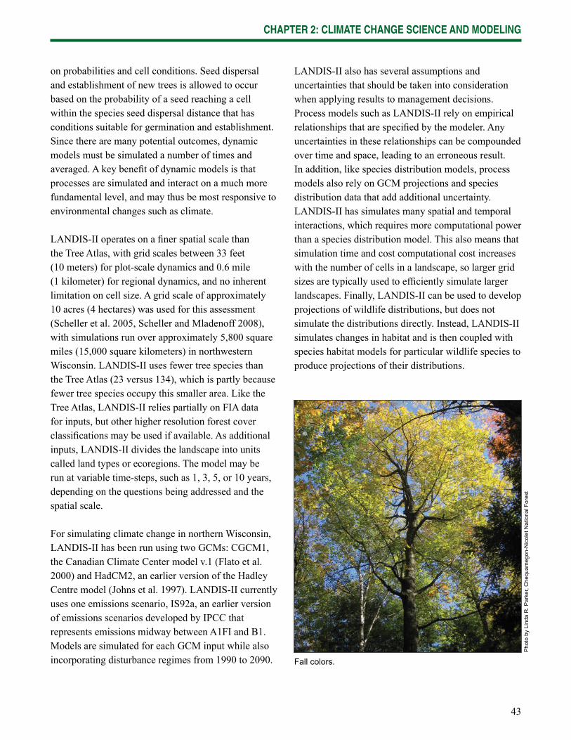
CHAPTER 2: CLIMATE CHANGE SCIENCE AND MODELING
43
on probabilities and cell conditions. Seed dispersal and establishment of new trees is allowed to occur based on the probability of a seed reaching a cell within the species seed dispersal distance that has conditions suitable for germination and establishment. Since there are many potential outcomes, dynamic models must be simulated a number of times and averaged. A key benefi t of dynamic models is that processes are simulated and interact on a much more fundamental level, and may thus be most responsive to environmental changes such as climate.
LANDIS-II operates on a fi ner spatial scale than the Tree Atlas, with grid scales between 33 feet (10 meters) for plot-scale dynamics and 0.6 mile (1 kilometer) for regional dynamics, and no inherent limitation on cell size. A grid scale of approximately 10 acres (4 hectares) was used for this assessment (Scheller et al. 2005, Scheller and Mladenoff 2008), with simulations run over approximately 5,800 square miles (15,000 square kilometers) in northwestern Wisconsin. LANDIS-II uses fewer tree species than the Tree Atlas (23 versus 134), which is partly because fewer tree species occupy this smaller area. Like the Tree Atlas, LANDIS-II relies partially on FIA data for inputs, but other higher resolution forest cover classifi cations may be used if available. As additional inputs, LANDIS-II divides the landscape into units called land types or ecoregions. The model may be run at variable time-steps, such as 1, 3, 5, or 10 years, depending on the questions being addressed and the spatial scale.
For simulating climate change in northern Wisconsin, LANDIS-II has been run using two GCMs: CGCM1, the Canadian Climate Center model v.1 (Flato et al. 2000) and HadCM2, an earlier version of the Hadley Centre model (Johns et al. 1997). LANDIS-II currently uses one emissions scenario, IS92a, an earlier version of emissions scenarios developed by IPCC that represents emissions midway between A1FI and B1. Models are simulated for each GCM input while also incorporating disturbance regimes from 1990 to 2090.
LANDIS-II also has several assumptions and uncertainties that should be taken into consideration when applying results to management decisions. Process models such as LANDIS-II rely on empirical relationships that are specifi ed by the modeler. Any uncertainties in these relationships can be compounded over time and space, leading to an erroneous result. In addition, like species distribution models, process models also rely on GCM projections and species distribution data that add additional uncertainty. LANDIS-II has simulates many spatial and temporal interactions, which requires more computational power than a species distribution model. This also means that simulation time and cost computational cost increases with the number of cells in a landscape, so larger grid sizes are typically used to effi ciently simulate larger landscapes. Finally, LANDIS-II can be used to develop projections of wildlife distributions, but does not simulate the distributions directly. Instead, LANDIS-II simulates changes in habitat and is then coupled with species habitat models for particular wildlife species to produce projections of their distributions.
Fall colors.
Pho
to b
y Li
nda
R. P
arke
r, C
hequ
ameg
on-N
icol
et N
atio
nal F
ores
t
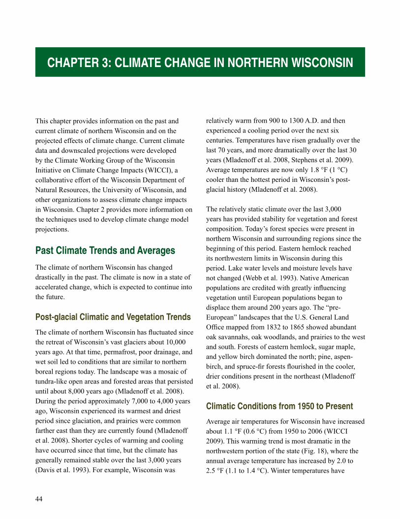
44
CHAPTER 3: CLIMATE CHANGE IN NORTHERN WISCONSIN
This chapter provides information on the past and current climate of northern Wisconsin and on the projected effects of climate change. Current climate data and downscaled projections were developed by the Climate Working Group of the Wisconsin Initiative on Climate Change Impacts (WICCI), a collaborative effort of the Wisconsin Department of Natural Resources, the University of Wisconsin, and other organizations to assess climate change impacts in Wisconsin. Chapter 2 provides more information on the techniques used to develop climate change model projections.
Past Climate Trends and Averages
The climate of northern Wisconsin has changed drastically in the past. The climate is now in a state of accelerated change, which is expected to continue into the future.
Post-glacial Climatic and Vegetation Trends
The climate of northern Wisconsin has fl uctuated since the retreat of Wisconsin’s vast glaciers about 10,000 years ago. At that time, permafrost, poor drainage, and wet soil led to conditions that are similar to northern boreal regions today. The landscape was a mosaic of tundra-like open areas and forested areas that persisted until about 8,000 years ago (Mladenoff et al. 2008). During the period approximately 7,000 to 4,000 years ago, Wisconsin experienced its warmest and driest period since glaciation, and prairies were common farther east than they are currently found (Mladenoff et al. 2008). Shorter cycles of warming and cooling have occurred since that time, but the climate has generally remained stable over the last 3,000 years (Davis et al. 1993). For example, Wisconsin was
relatively warm from 900 to 1300 A.D. and then experienced a cooling period over the next six centuries. Temperatures have risen gradually over the last 70 years, and more dramatically over the last 30 years (Mladenoff et al. 2008, Stephens et al. 2009). Average temperatures are now only 1.8 °F (1 °C) cooler than the hottest period in Wisconsin’s post-glacial history (Mladenoff et al. 2008).
The relatively static climate over the last 3,000 years has provided stability for vegetation and forest composition. Today’s forest species were present in northern Wisconsin and surrounding regions since the beginning of this period. Eastern hemlock reached its northwestern limits in Wisconsin during this period. Lake water levels and moisture levels have not changed (Webb et al. 1993). Native American populations are credited with greatly infl uencing vegetation until European populations began to displace them around 200 years ago. The “pre-European” landscapes that the U.S. General Land Offi ce mapped from 1832 to 1865 showed abundant oak savannahs, oak woodlands, and prairies to the west and south. Forests of eastern hemlock, sugar maple, and yellow birch dominated the north; pine, aspen-birch, and spruce-fi r forests fl ourished in the cooler, drier conditions present in the northeast (Mladenoff et al. 2008).
Climatic Conditions from 1950 to Present
Average air temperatures for Wisconsin have increased about 1.1 °F (0.6 °C) from 1950 to 2006 (WICCI 2009). This warming trend is most dramatic in the northwestern portion of the state (Fig. 18), where the annual average temperature has increased by 2.0 to 2.5 °F (1.1 to 1.4 °C). Winter temperatures have

45
CHAPTER 3: CLIMATE CHANGE IN NORTHERN WISCONSIN
increased by 2.5 °F (1.4 °C) statewide and 3.5 to 4.5 °F (1.9 to 2.5 °C) in the northwest. Spring temperatures have increased by 1.7 °F (0.9 °C) statewide and 2.5 to 3.5 °F (1.4-1.9 °C) in the northwest. Summer temperatures show the least amount of warming, with a statewide increase of 0.5 °F (0.3 °C), although more substantial temperature increases of 1.5 to 2.0 °F (0.8 to 1.1 °C) have been measured in the central northwest. Autumn daytime temperatures in Wisconsin have exhibited a cooling trend (-0.6 °F; -0.3 °C), especially in the northeast and far southwest portions of the state where average temperatures have dropped by 1.5 °F (0.8 °C; Kucharik et al. 2010).
Precipitation patterns have also changed (Fig. 19). Statewide average rainfall increased by 3.1 inches (78.7 mm) from 1950 to 2006 (WICCI 2009). Most of the increase has been concentrated in southern and western Wisconsin, with increases ranging from 2 to 4 inches (50 to 100 mm) since 1950 (Kucharik et al. 2010). Northern Wisconsin, however, has become drier, with the annual average decreasing by 0.8 to 2.4 inches (20 to 60 mm) during this time period
(Kucharik et al. 2010). The intensity and frequency of precipitation events are increasing across the state and the entire Midwest, which has experienced a doubling of heavy downpours compared to a century ago (Karl et al. 2009) and a 50 percent increase in the frequency of days with more than 4 inches (101.6 mm) of precipitation. Events on the all-time record rainfall list are quickly being replaced by record rainfalls of the past 20 years. Two record-breaking fl oods occurred in the Midwest in 1993 and 2008 (Karl et al. 2009).
Ice cover on the Great Lakes is directly related to the number and intensity of below-freezing days. The average date of ice breakup for Wisconsin lakes has become signifi cantly earlier, especially for smaller lakes (Robertson et al. 1992). An increase in air temperature of 1.8 °F (1 °C) shortens ice duration by more than 10 days (Robertson et al. 1992). Magnuson et al. (2000) demonstrated a similar trend on other small lakes in North America using at least 100 years of data. Over a 100 year period, North American lakes break up 1.3 days earlier every decade, and accelerated warming since 1950 is refl ected by a decrease in ice cover of 6.4 days per decade.
Figure 18.—Observed changes in temperature (°F) from 1950 to 2006 during the winter (A) and summer (B) seasons. Figure courtesy of the Wisconsin Initiative on Climate Change Impacts (WICCI 2009).
A B
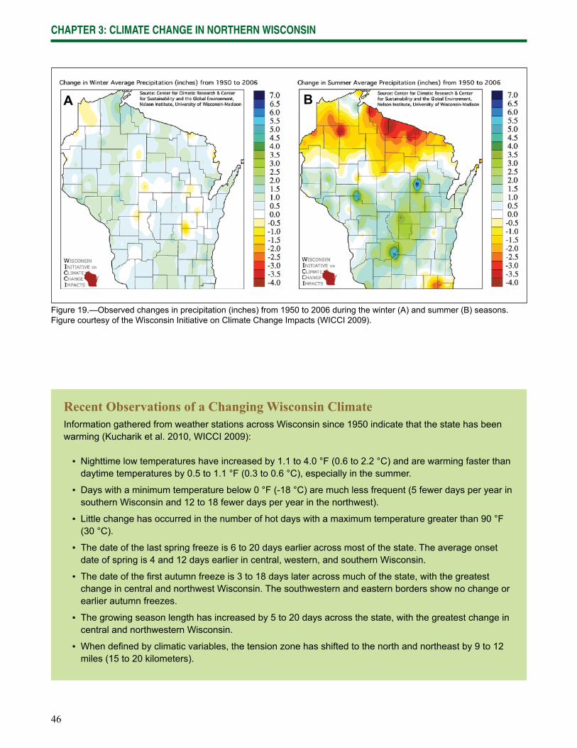
46
CHAPTER 3: CLIMATE CHANGE IN NORTHERN WISCONSIN
Recent Observations of a Changing Wisconsin ClimateInformation gathered from weather stations across Wisconsin since 1950 indicate that the state has been warming (Kucharik et al. 2010, WICCI 2009):
▪ Nighttime low temperatures have increased by 1.1 to 4.0 °F (0.6 to 2.2 °C) and are warming faster than daytime temperatures by 0.5 to 1.1 °F (0.3 to 0.6 °C), especially in the summer.
▪ Days with a minimum temperature below 0 °F (-18 °C) are much less frequent (5 fewer days per year in southern Wisconsin and 12 to 18 fewer days per year in the northwest).
▪ Little change has occurred in the number of hot days with a maximum temperature greater than 90 °F (30 °C).
▪ The date of the last spring freeze is 6 to 20 days earlier across most of the state. The average onset date of spring is 4 and 12 days earlier in central, western, and southern Wisconsin.
▪ The date of the fi rst autumn freeze is 3 to 18 days later across much of the state, with the greatest change in central and northwest Wisconsin. The southwestern and eastern borders show no change or earlier autumn freezes.
▪ The growing season length has increased by 5 to 20 days across the state, with the greatest change in central and northwestern Wisconsin.
▪ When defi ned by climatic variables, the tension zone has shifted to the north and northeast by 9 to 12 miles (15 to 20 kilometers).
Figure 19.—Observed changes in precipitation (inches) from 1950 to 2006 during the winter (A) and summer (B) seasons. Figure courtesy of the Wisconsin Initiative on Climate Change Impacts (WICCI 2009).
A B
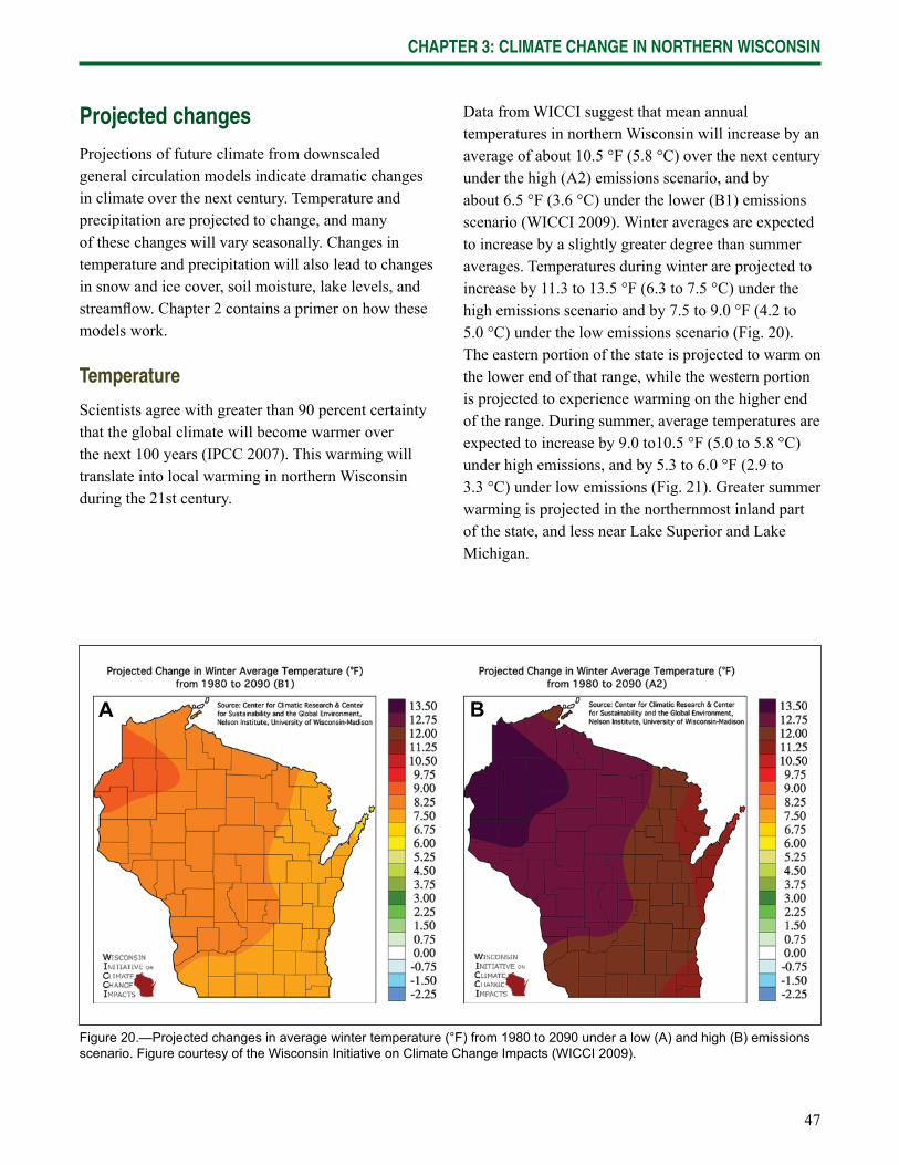
47
CHAPTER 3: CLIMATE CHANGE IN NORTHERN WISCONSIN
Projected changes
Projections of future climate from downscaled general circulation models indicate dramatic changes in climate over the next century. Temperature and precipitation are projected to change, and many of these changes will vary seasonally. Changes in temperature and precipitation will also lead to changes in snow and ice cover, soil moisture, lake levels, and streamfl ow. Chapter 2 contains a primer on how these models work.
Temperature
Scientists agree with greater than 90 percent certainty that the global climate will become warmer over the next 100 years (IPCC 2007). This warming will translate into local warming in northern Wisconsin during the 21st century.
Data from WICCI suggest that mean annual temperatures in northern Wisconsin will increase by an average of about 10.5 °F (5.8 °C) over the next century under the high (A2) emissions scenario, and by about 6.5 °F (3.6 °C) under the lower (B1) emissions scenario (WICCI 2009). Winter averages are expected to increase by a slightly greater degree than summer averages. Temperatures during winter are projected to increase by 11.3 to 13.5 °F (6.3 to 7.5 °C) under the high emissions scenario and by 7.5 to 9.0 °F (4.2 to 5.0 °C) under the low emissions scenario (Fig. 20). The eastern portion of the state is projected to warm on the lower end of that range, while the western portion is projected to experience warming on the higher end of the range. During summer, average temperatures are expected to increase by 9.0 to10.5 °F (5.0 to 5.8 °C) under high emissions, and by 5.3 to 6.0 °F (2.9 to 3.3 °C) under low emissions (Fig. 21). Greater summer warming is projected in the northernmost inland part of the state, and less near Lake Superior and Lake Michigan.
Figure 20.—Projected changes in average winter temperature (°F) from 1980 to 2090 under a low (A) and high (B) emissions scenario. Figure courtesy of the Wisconsin Initiative on Climate Change Impacts (WICCI 2009).
A B
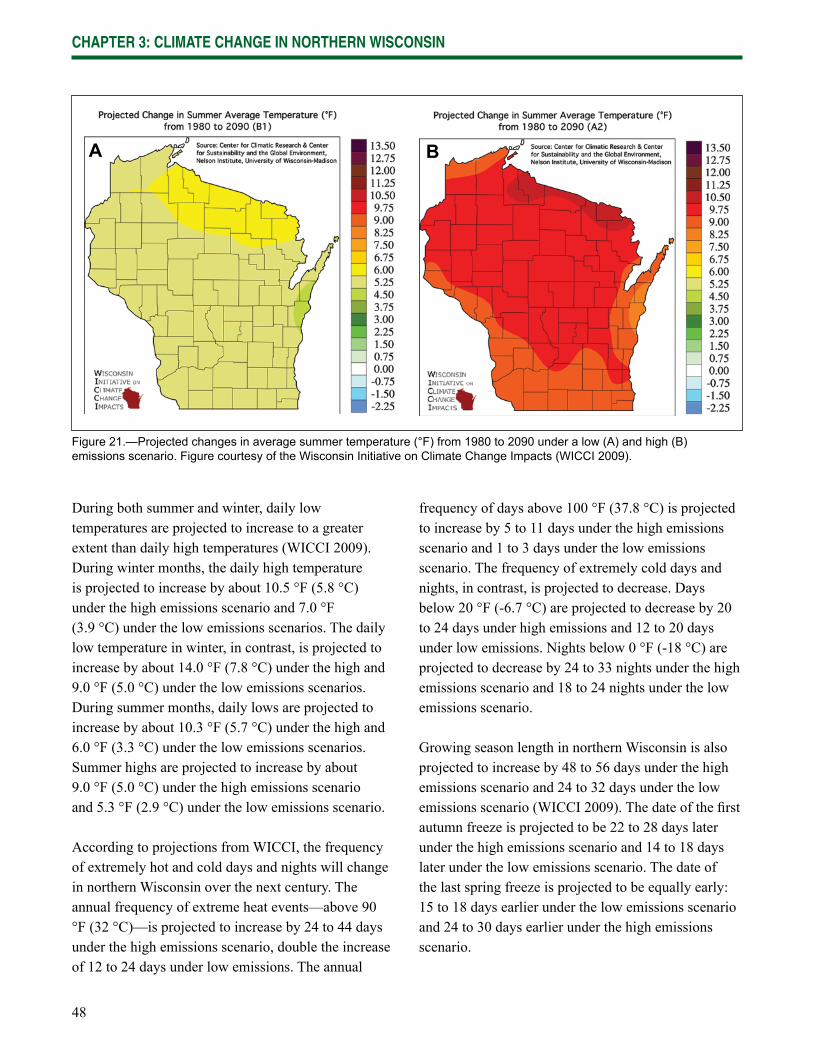
48
CHAPTER 3: CLIMATE CHANGE IN NORTHERN WISCONSIN
Figure 21.—Projected changes in average summer temperature (°F) from 1980 to 2090 under a low (A) and high (B) emissions scenario. Figure courtesy of the Wisconsin Initiative on Climate Change Impacts (WICCI 2009).
A B
During both summer and winter, daily low temperatures are projected to increase to a greater extent than daily high temperatures (WICCI 2009). During winter months, the daily high temperature is projected to increase by about 10.5 °F (5.8 °C) under the high emissions scenario and 7.0 °F (3.9 °C) under the low emissions scenarios. The daily low temperature in winter, in contrast, is projected to increase by about 14.0 °F (7.8 °C) under the high and 9.0 °F (5.0 °C) under the low emissions scenarios. During summer months, daily lows are projected to increase by about 10.3 °F (5.7 °C) under the high and 6.0 °F (3.3 °C) under the low emissions scenarios. Summer highs are projected to increase by about 9.0 °F (5.0 °C) under the high emissions scenario and 5.3 °F (2.9 °C) under the low emissions scenario.
According to projections from WICCI, the frequency of extremely hot and cold days and nights will change in northern Wisconsin over the next century. The annual frequency of extreme heat events—above 90 °F (32 °C)—is projected to increase by 24 to 44 days under the high emissions scenario, double the increase of 12 to 24 days under low emissions. The annual
frequency of days above 100 °F (37.8 °C) is projected to increase by 5 to 11 days under the high emissions scenario and 1 to 3 days under the low emissions scenario. The frequency of extremely cold days and nights, in contrast, is projected to decrease. Days below 20 °F (-6.7 °C) are projected to decrease by 20 to 24 days under high emissions and 12 to 20 days under low emissions. Nights below 0 °F (-18 °C) are projected to decrease by 24 to 33 nights under the high emissions scenario and 18 to 24 nights under the low emissions scenario.
Growing season length in northern Wisconsin is also projected to increase by 48 to 56 days under the high emissions scenario and 24 to 32 days under the low emissions scenario (WICCI 2009). The date of the fi rst autumn freeze is projected to be 22 to 28 days later under the high emissions scenario and 14 to 18 days later under the low emissions scenario. The date of the last spring freeze is projected to be equally early: 15 to 18 days earlier under the low emissions scenario and 24 to 30 days earlier under the high emissions scenario.
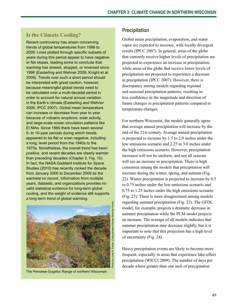
49
CHAPTER 3: CLIMATE CHANGE IN NORTHERN WISCONSIN
Is the Climate Cooling?Recent controversy has arisen concerning trends of global temperatures from 1998 to 2009. Lines plotted through specifi c subsets of years during this period appear to have negative or fl at slopes, leading some to conclude that warming has slowed, stopped, or reversed since 1998 (Easterling and Wehner 2009, Knight et al. 2009). Trends over such a short period should be interpreted with great caution, however, because meaningful global trends need to be calculated over a multi-decadal period in order to account for natural annual variation in the Earth’s climate (Easterling and Wehner 2009, IPCC 2007). Global mean temperature can increase or decrease from year to year because of volcanic eruptions, solar activity, and large-scale ocean circulation patterns like El Niño. Since 1880 there have been several 5- to 10-year periods during which trends appeared to be fl at or even negative, including a long, level period from the 1940s to the 1970s. Nonetheless, the overall trend has been positive, and recent decades are clearly warmer than preceding decades (Chapter 2, Fig. 10). In fact, the NASA Goddard Institute for Space Studies (2010) has recently ranked the decade from January 2000 to December 2009 as the warmest on record. Information from multiple years, datasets, and organizations provides no valid statistical evidence for long-term global cooling, and the weight of evidence still supports a long-term trend of global warming.
The Penokee-Gogebic Range of northern Wisconsin.
Pho
to b
y Li
nda
R. P
arke
r, C
hequ
ameg
on-N
icol
et N
atio
nal F
ores
t
Precipitation
Global mean precipitation, evaporation, and water vapor are expected to increase, with locally divergent results (IPCC 2007). In general, areas of the globe that currently receive higher levels of precipitation are projected to experience an increase in precipitation, while areas of the globe that receive lower levels of precipitation are projected to experience a decrease in precipitation (IPCC 2007). However, there is discrepancy among models regarding regional and seasonal precipitation patterns, resulting in less confi dence in the magnitude and direction of future changes in precipitation patterns compared to temperature changes.
For northern Wisconsin, the models generally agree that average annual precipitation will increase by the end of the 21st century. Average annual precipitation is projected to increase by 1.5 to 2.0 inches under the low emissions scenario and 2.25 to 3.0 inches under the high emissions scenario. However, precipitation increases will not be uniform, and not all seasons will see an increase in precipitation. There is high consensus among the models that precipitation will increase during the winter, spring, and autumn (Fig. 22). Winter precipitation is projected to increase by 0.5 to 0.75 inches under the low emissions scenario and 0.75 to 1.25 inches under the high emissions scenario (Fig. 23). There is more disagreement among models regarding summer precipitation (Fig. 22). The GFDL model, for example, projects a dramatic decrease in summer precipitation while the PCM model projects an increase. The average of all models indicates that summer precipitation may decrease slightly, but it is important to note that this projection has a high level of uncertainty (Fig. 24).
Heavy precipitation events are likely to become more frequent, especially in areas that experience lake-effect precipitation (WICCI 2009). The number of days per decade where greater than one inch of precipitation
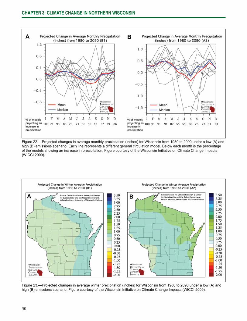
50
CHAPTER 3: CLIMATE CHANGE IN NORTHERN WISCONSIN
Figure 22.—Projected changes in average monthly precipitation (inches) for Wisconsin from 1980 to 2090 under a low (A) and high (B) emissions scenario. Each line represents a different general circulation model. Below each month is the percentage of the models showing an increase in precipitation. Figure courtesy of the Wisconsin Initiative on Climate Change Impacts (WICCI 2009).
Figure 23.—Projected changes in average winter precipitation (inches) for Wisconsin from 1980 to 2090 under a low (A) and high (B) emissions scenario. Figure courtesy of the Wisconsin Initiative on Climate Change Impacts (WICCI 2009).
A B
A B
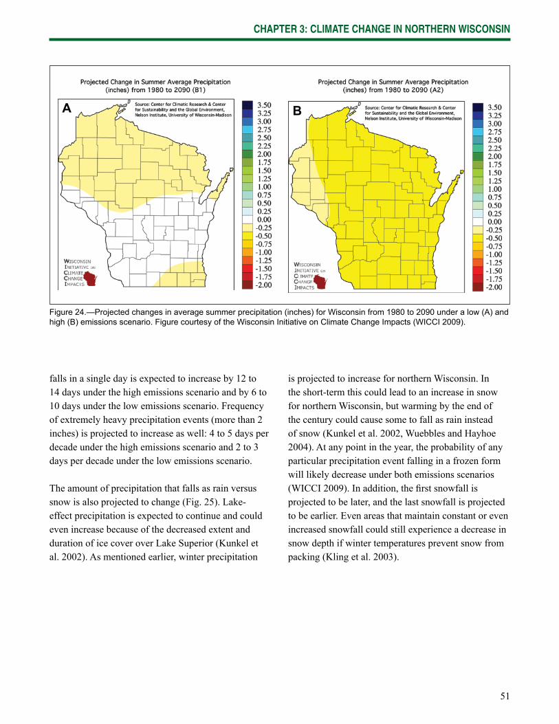
51
CHAPTER 3: CLIMATE CHANGE IN NORTHERN WISCONSIN
falls in a single day is expected to increase by 12 to 14 days under the high emissions scenario and by 6 to 10 days under the low emissions scenario. Frequency of extremely heavy precipitation events (more than 2 inches) is projected to increase as well: 4 to 5 days per decade under the high emissions scenario and 2 to 3 days per decade under the low emissions scenario.
The amount of precipitation that falls as rain versus snow is also projected to change (Fig. 25). Lake-effect precipitation is expected to continue and could even increase because of the decreased extent and duration of ice cover over Lake Superior (Kunkel et al. 2002). As mentioned earlier, winter precipitation
Figure 24.—Projected changes in average summer precipitation (inches) for Wisconsin from 1980 to 2090 under a low (A) and high (B) emissions scenario. Figure courtesy of the Wisconsin Initiative on Climate Change Impacts (WICCI 2009).
A B
is projected to increase for northern Wisconsin. In the short-term this could lead to an increase in snow for northern Wisconsin, but warming by the end of the century could cause some to fall as rain instead of snow (Kunkel et al. 2002, Wuebbles and Hayhoe 2004). At any point in the year, the probability of any particular precipitation event falling in a frozen form will likely decrease under both emissions scenarios (WICCI 2009). In addition, the fi rst snowfall is projected to be later, and the last snowfall is projected to be earlier. Even areas that maintain constant or even increased snowfall could still experience a decrease in snow depth if winter temperatures prevent snow from packing (Kling et al. 2003).
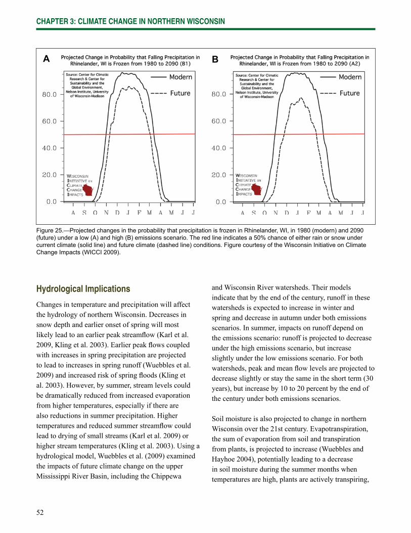
52
CHAPTER 3: CLIMATE CHANGE IN NORTHERN WISCONSIN
Figure 25.—Projected changes in the probability that precipitation is frozen in Rhinelander, WI, in 1980 (modern) and 2090 (future) under a low (A) and high (B) emissions scenario. The red line indicates a 50% chance of either rain or snow under current climate (solid line) and future climate (dashed line) conditions. Figure courtesy of the Wisconsin Initiative on Climate Change Impacts (WICCI 2009).
A B
Hydrological Implications
Changes in temperature and precipitation will affect the hydrology of northern Wisconsin. Decreases in snow depth and earlier onset of spring will most likely lead to an earlier peak streamfl ow (Karl et al. 2009, Kling et al. 2003). Earlier peak fl ows coupled with increases in spring precipitation are projected to lead to increases in spring runoff (Wuebbles et al. 2009) and increased risk of spring fl oods (Kling et al. 2003). However, by summer, stream levels could be dramatically reduced from increased evaporation from higher temperatures, especially if there are also reductions in summer precipitation. Higher temperatures and reduced summer streamfl ow could lead to drying of small streams (Karl et al. 2009) or higher stream temperatures (Kling et al. 2003). Using a hydrological model, Wuebbles et al. (2009) examined the impacts of future climate change on the upper Mississippi River Basin, including the Chippewa
and Wisconsin River watersheds. Their models indicate that by the end of the century, runoff in these watersheds is expected to increase in winter and spring and decrease in autumn under both emissions scenarios. In summer, impacts on runoff depend on the emissions scenario: runoff is projected to decrease under the high emissions scenario, but increase slightly under the low emissions scenario. For both watersheds, peak and mean fl ow levels are projected to decrease slightly or stay the same in the short term (30 years), but increase by 10 to 20 percent by the end of the century under both emissions scenarios.
Soil moisture is also projected to change in northern Wisconsin over the 21st century. Evapotranspiration, the sum of evaporation from soil and transpiration from plants, is projected to increase (Wuebbles and Hayhoe 2004), potentially leading to a decrease in soil moisture during the summer months when temperatures are high, plants are actively transpiring,
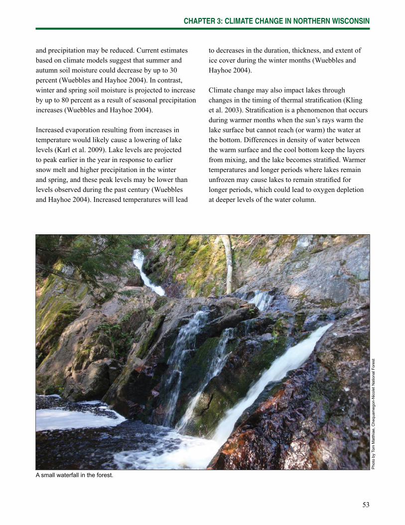
53
CHAPTER 3: CLIMATE CHANGE IN NORTHERN WISCONSIN
and precipitation may be reduced. Current estimates based on climate models suggest that summer and autumn soil moisture could decrease by up to 30 percent (Wuebbles and Hayhoe 2004). In contrast, winter and spring soil moisture is projected to increase by up to 80 percent as a result of seasonal precipitation increases (Wuebbles and Hayhoe 2004).
Increased evaporation resulting from increases in temperature would likely cause a lowering of lake levels (Karl et al. 2009). Lake levels are projected to peak earlier in the year in response to earlier snow melt and higher precipitation in the winter and spring, and these peak levels may be lower than levels observed during the past century (Wuebbles and Hayhoe 2004). Increased temperatures will lead
to decreases in the duration, thickness, and extent of ice cover during the winter months (Wuebbles and Hayhoe 2004).
Climate change may also impact lakes through changes in the timing of thermal stratifi cation (Kling et al. 2003). Stratifi cation is a phenomenon that occurs during warmer months when the sun’s rays warm the lake surface but cannot reach (or warm) the water at the bottom. Differences in density of water between the warm surface and the cool bottom keep the layers from mixing, and the lake becomes stratifi ed. Warmer temperatures and longer periods where lakes remain unfrozen may cause lakes to remain stratifi ed for longer periods, which could lead to oxygen depletion at deeper levels of the water column.
A small waterfall in the forest.
Pho
to b
y To
m M
atth
iae,
Che
quam
egon
-Nic
olet
Nat
iona
l For
est
54
CHAPTER 4: CLIMATE CHANGE EFFECTS ON FORESTS
Climate change will alter the forested ecosystems of northern Wisconsin. The most visible changes may initially be in forest health and vigor, although fundamental changes in ecosystem function, structure, and species distribution will likely become increasingly evident. Other important physical and biological characteristics of ecosystems, such as soil and water quality, carbon storage and nutrient cycling, and wildlife habitat type and quality, may not be as readily apparent (Anderson et al. 1976, Ice and Stednick 2004, Waring and Schlesinger 1985).
This chapter describes the effects of climate change on some of these forest ecosystem characteristics, with an emphasis on the expected changes in tree species abundance and composition. Two different modeling approaches were used to simulate climate change impacts on forests, a species distribution model (The Tree Atlas) and a process model (LANDIS-II), and the results from these two modeling approaches are summarized.
Climate Change and Forests
Climate change is expected to impact both entire forest ecosystems and the individual tree species that compose forest communities. Projected increases in annual mean temperature, increased variability in precipitation and soil moisture balance, and increases in atmospheric carbon dioxide will have direct and indirect effects on multiple, interconnected ecosystem components and drivers. In Wisconsin and the Midwest, climate change is expected to result in increased likelihood of periodic drought conditions, fl ash fl ooding, and extreme weather events (UCS 2009). Disturbances are expected to increase,
including severe wind events (Frelich and Reich 2010). Within forests, the climatological changes and increased disturbance will interact with natural processes to increase the intensity and duration of stress. For example, the combined effects of drought conditions, longer growing seasons, and increased temperatures will likely intensify fi re regimes (frequency, severity, and season length) and increase insect infestation (frequency, duration, and extent; Soja et al. 2007). Additionally, a number of vital soil processes will be altered, including nutrient cycling, carbon storage, decomposition, and water storage and recharge. Importantly, all of these new stressors will occur in addition to existing stressors, such as pathogens and insects, competition from invasive species, and ozone and other pollution. Cascading interactions of stressors in these systems threaten to reduce productivity further and can even cause mortality as trees become less vigorous and resilient (Aber et al. 2001).
Trees and other plant species have responded to past climate change in a number of ways and at a number of spatial scales (Ritchie 1986). The ranges of tree species in eastern North America have generally shifted northward as the climate has warmed over the past 14,000+ years since the last ice age (Davis 1981, Delcourt and Delcourt 1987, Webb et al. 1987). Evidence is mounting that tree species, along with many other organisms, are currently moving northward (Parmesan and Yohe 2003, Woodall et al. 2009) and upward in elevation (Lee et al. 2005), with some species migrating at very high rates (Woodall et al. 2009). Such shifts are likely to continue and even accelerate in the coming decades in Wisconsin as habitat suitability changes, resulting in declines in
55
CHAPTER 4: CLIMATE CHANGE EFFECTS ON FORESTS
species abundance or productivity, or even the loss of entire species from certain areas. Past disturbances, habitat fragmentation or loss, and management practices already prevent species from occupying all suitable habitat within their ranges. If climate change were to further decrease the suitable habitat of major species in conjunction with these other effects, then overall forest abundance or density would decrease and forest productivity declines would be exacerbated (Aber et al. 2001, Hanson and Weltzin 2000).
New conditions may be suitable for other species, however, leading to successional shifts and changing forest composition over time. Elevated carbon dioxide may actually enhance the growth of some species (Norby et al. 2005) and increase their water use effi ciency (Ainsworth and Rogers 2007), potentially offsetting the effects of drier growing seasons. There is already some evidence for increased forest growth globally (Bonan 2008) and in the eastern United States (Cole et al. 2010, McMahon et al. 2010), but the issue question is still under active discussion (Bonan 2008, Foster et al. 2010) and it remains unclear if long-term enhanced growth can be sustained. Nutrient and water availability, ozone pollution, and tree age and size all play major roles in the ability of trees to capitalize on carbon dioxide fertilization (Ainsworth and Long 2005). Ecosystem community shifts may take place as some species are genetically better able to take advantage of carbon dioxide fertilization than others (Souza et al. 2010).
Other community shifts may result from plant migration. It is possible that some species that are currently considerably distant from northern Wisconsin will migrate into the region, even as resident species disappear. However, it is important to note that migration of new species is constrained by a number of factors, including seed dispersal dynamics and landscape fragmentation, and it is expected that species will not be able to migrate northward without substantially lagging behind changes in climate (Iverson et al. 2004a,b; Scheller and Mladenoff 2008).
The Climate Change Tree Atlas
The Climate Change Tree Atlas is one of two approaches that were used to understand the potential impacts of climate change on forests in northern Wisconsin (Chapter 2, Appendix 4; Iverson et al. 2008a,b). The Tree Atlas uses an ensemble of species distribution models to examine the features that contribute to a tree species’ current habitat and then project where similar habitat conditions are likely to occur in the future. The Tree Atlas does not predict where species will be present in the future, but rather where suitable habitat for individual tree species may be present.
For this assessment, the Tree Atlas examined the location of potential suitable habitat for 73 tree species that currently are present in northern Wisconsin or are predicted to have suitable habitat in the future. The results of this analysis show that climate change will likely lead to changes in the suitable habitat of many common tree species. The ways in which tree species will actually respond to climate change, however, is infl uenced by a number of “modifying factors” including site conditions, competition from other species, landscape connectivity, the degree of disturbance, and the ability of species to disperse, many of which cannot be modeled directly by the Tree Atlas. To fi ll these gaps, we used additional information from the research literature and examined the individual models to assess the unique ways in which individual species may respond to climate change. When practical, the contributions of these modifying factors have been included, with more details presented in Appendix 4.
Of 134 species modeled in the eastern United States by the Tree Atlas (Prasad et al. 2007), 73 are of interest for this assessment because they currently have or are projected to have suitable habitat under future conditions in northern Wisconsin. A number of projections of future climate were used in the modeling, and results are reported using a low
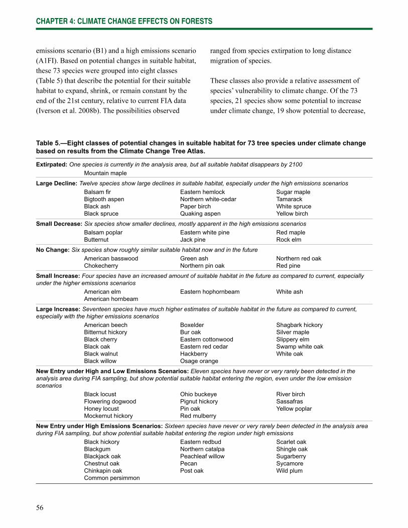
56
CHAPTER 4: CLIMATE CHANGE EFFECTS ON FORESTS
emissions scenario (B1) and a high emissions scenario (A1FI). Based on potential changes in suitable habitat, these 73 species were grouped into eight classes (Table 5) that describe the potential for their suitable habitat to expand, shrink, or remain constant by the end of the 21st century, relative to current FIA data (Iverson et al. 2008b). The possibilities observed
ranged from species extirpation to long distance migration of species.
These classes also provide a relative assessment of species’ vulnerability to climate change. Of the 73 species, 21 species show some potential to increase under climate change, 19 show potential to decrease,
Table 5.—Eight classes of potential changes in suitable habitat for 73 tree species under climate change based on results from the Climate Change Tree Atlas.
Extirpated: One species is currently in the analysis area, but all suitable habitat disappears by 2100 Mountain maple
Large Decline: Twelve species show large declines in suitable habitat, especially under the high emissions scenarios Balsam fi r Eastern hemlock Sugar maple Bigtooth aspen Northern white-cedar Tamarack Black ash Paper birch White spruce Black spruce Quaking aspen Yellow birch
Small Decrease: Six species show smaller declines, mostly apparent in the high emissions scenarios Balsam poplar Eastern white pine Red maple Butternut Jack pine Rock elm
No Change: Six species show roughly similar suitable habitat now and in the future American basswood Green ash Northern red oak Chokecherry Northern pin oak Red pine
Small Increase: Four species have an increased amount of suitable habitat in the future as compared to current, especially under the higher emissions scenarios American elm Eastern hophornbeam White ash American hornbeam
Large Increase: Seventeen species have much higher estimates of suitable habitat in the future as compared to current, especially with the higher emissions scenarios American beech Boxelder Shagbark hickory Bitternut hickory Bur oak Silver maple Black cherry Eastern cottonwood Slippery elm Black oak Eastern red cedar Swamp white oak Black walnut Hackberry White oak Black willow Osage orange
New Entry under High and Low Emissions Scenarios: Eleven species have never or very rarely been detected in the analysis area during FIA sampling, but show potential suitable habitat entering the region, even under the low emission scenarios Black locust Ohio buckeye River birch Flowering dogwood Pignut hickory Sassafras Honey locust Pin oak Yellow poplar Mockernut hickory Red mulberry
New Entry under High Emissions Scenarios: Sixteen species have never or very rarely been detected in the analysis area during FIA sampling, but show potential suitable habitat entering the region under high emissions Black hickory Eastern redbud Scarlet oak Blackgum Northern catalpa Shingle oak Blackjack oak Peachleaf willow Sugarberry Chestnut oak Pecan Sycamore Chinkapin oak Post oak Wild plum Common persimmon
57
CHAPTER 4: CLIMATE CHANGE EFFECTS ON FORESTS
6 show little or no change, and another 27 species show the potential for some level of new suitable habitat entering the region under at least the high emissions scenario.
Loss of Suitable Habitat
In the Tree Atlas analysis, mountain maple was the only species to fall into this class. Mountain maple is a predominantly northern species, and in northern Wisconsin it is typically found in the understory of northern hardwoods and other mesic forest types. Data from FIA (Miles 2010) sampling indicates that the species is very uncommon now. Loss of suitable habitat was projected under both low and high emissions scenarios. Further analysis of the Tree Atlas indicates that the model for mountain maple has a high degree of reliability, and that the species is probably quite sensitive to temperature changes. However, examination of both the disturbance and biological modifying factors suggests that the species could do somewhat better than the models suggest.
Large Declines in Suitable Habitat
The Tree Atlas identifi ed 12 species that are projected to have large declines in potential suitable habitat: black spruce, balsam fi r, northern white-cedar, yellow birch, paper birch, quaking aspen, white spruce, eastern hemlock, sugar maple, black ash, tamarack, and bigtooth aspen. Many of these species are very common and important in the forests of northern Wisconsin. Additionally, partly due to the high frequency of these species in the region, all but one, white spruce, have high model reliability scores.
Black spruce—Black spruce is second only to mountain maple in projected suitable habitat decreases. The model predicts suitable habitat for black spruce being reduced to 13 percent of its current habitat under the low emissions scenario and 8 percent under the high emissions scenario. Black spruce also appears to be highly sensitive to the disturbances that are expected to increase in a warmer climate—especially
drought, insect pests, and fi re—suggesting the species may do worse than indicated by the habitat modeling. Although somewhat benefi ted by biological factors, especially shade tolerance, black spruce may be the most at risk among all species in northern Wisconsin.
Balsam fi r—Although balsam fi r is similar to black spruce in its sensitivity to disturbance and climatic factors and is found in many of the same habitats, our assessment shows it may be slightly more resilient. The model predicts suitable habitat for balsam fi r being reduced to 18 percent of current habitat under the low emissions scenarios and 9 percent under the high emissions scenario.
Northern white-cedar—Northern white-cedar is projected to have substantial reductions in suitable habitat, with habitat at the end of the century being reduced to 37 percent of current habitat under the high emissions scenario and 23 percent under the low emissions scenario.
Quaking aspen—Quaking aspen currently has the highest importance value (a measure of relative abundance) in all of northern Wisconsin and is found throughout the region. Although quaking aspen is projected to remain widespread, habitat is projected to decline to 45 percent of current habitat under the low emissions scenario and 17 percent under the high emissions scenario. Several modifi cation factors indicate that this species may do better than the habitat model predicts, including its ability to persist over large areas, broad temperature tolerances, cloning ability, and resilience to disturbance.
Paper birch—Currently ranked as fourth in importance value, paper birch suitable habitat is projected to decrease to 42 percent of current habitat under the low emissions scenario and 13 percent under the high emissions scenario. This projected loss may be exacerbated by negative response to drought and fi re topkill.
58
CHAPTER 4: CLIMATE CHANGE EFFECTS ON FORESTS
Bigtooth aspen—Bigtooth aspen has a projected habitat response that is greatly dependent on the emissions scenario. Under the low emissions scenario, a decline to 80 percent of current habitat is projected; whereas under the high emissions scenario, habitat is projected to decline to 25 percent of current habitat. This difference in response is caused by a greater northward shift in habitat that creates a greater loss of occupancy under higher emissions. Further analysis of the model indicates that the cooler and wetter environments may contain the habitats most likely to remain suitable for bigtooth aspen over the next century.
Sugar maple—Currently ranked third in importance value, sugar maple is found across the forests of northern Wisconsin. Although suitable habitat is projected to decline to 62 percent of current habitat under the low emissions scenario and to 31 percent under the high emissions scenario, sugar maple is likely to persist in areas where it is currently found (Fig. 26). Sugar maple has many characteristics, such as high shade tolerance and fewer disease and insect pests relative to other species, that indicate that this species may do better than projected in the habitat suitability models.
Yellow birch—Yellow birch habitat is projected to decline to 38 percent of current habitat under the low emissions and to 15 percent under the high emissions scenario (Fig. 26). The species’ high dispersal ability may be a benefi t under climate change, yet sensitivity to regional climate, fi re topkill, and insect pests suggest that the species may fare worse than projected by the model.
Eastern hemlock—The projected changes in suitable habitat for eastern hemlock vary substantially, with declines to 17 percent of its current habitat under the high emissions scenario and to 59 percent under the low emissions scenario. Along with the model results, consideration also has to be given to its susceptibility to hemlock wooly adelgid, a nonnative insect that is currently limited by cold winter temperatures but
may be able to invade and persist in the projected warmer climate (Paradis et al. 2008). Combined with the species’ negative response to drought, the adelgid (if introduced) may push the species’ decline beyond what was projected in the habitat model. Eastern hemlock is not a valuable timber species, but it has signifi cant ecological and aesthetic value. This species often grows in the lower, wetter areas along streams, and thus provides cooler habitats for many other organisms.
White spruce—White spruce habitat is projected to decline to 52 percent of current under the low emissions scenario and 39 percent under the high emissions scenario. Although the habitat model for white spruce had only moderate reliability (compared to high reliability for all other species projected to experience large habitat declines), additional examination of the species’ susceptibility to climate, disturbance, and other factors provide good evidence for a likely negative habitat response to climate change.
Black ash—Black ash suitable habitat is projected to decline to 69 percent of current under the low emissions scenario and 52 percent under the high emissions scenario. Despite the loss of suitable habitat, there is little projected change in the extent of the species’ occupancy, meaning that areas that are currently occupied are likely to remain occupied but at a lower level. The habitat model results for any ash species also need to be considered relative to the species’ high susceptibility to the nonnative emerald ash borer.
Tamarack—The model predicts suitable habitat for tamarack being reduced to 74 percent of current habitat under the low emissions scenario and to 53 percent under the high emissions scenario. However, tamarack is also projected to largely retain its occupancy despite these decreases. Unlike the other species in this class, tamarack appears to be more infl uenced by soil variables than by climatic variables. This resilience to changes in temperature is likely to support occupancy.
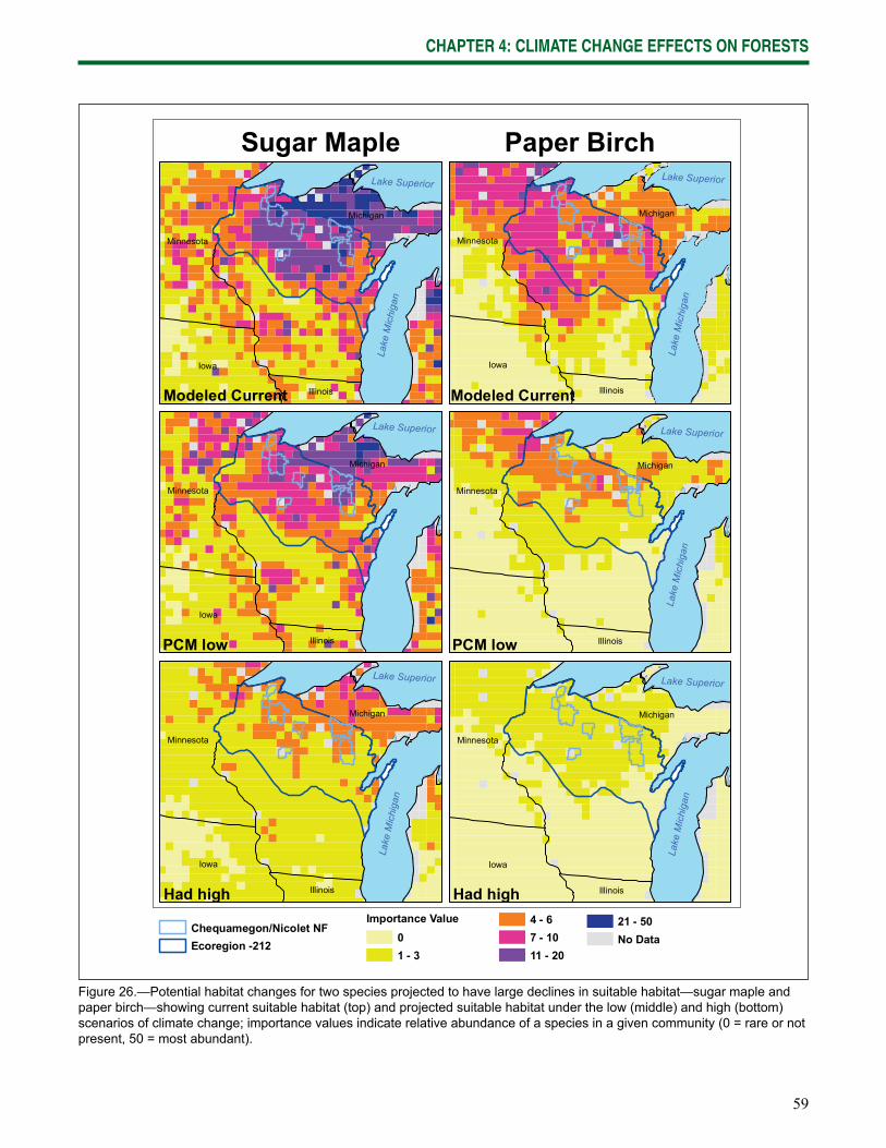
59
CHAPTER 4: CLIMATE CHANGE EFFECTS ON FORESTS
Chequamegon/Nicolet NFEcoregion -212
Importance Value01 - 3
4 - 67 - 1011 - 20
21 - 50No Data
Lake
Mic
higa
n
Lake Superior
Iowa
Minnesota
Michigan
Illinois
Sugar Maple Paper Birch
Lake Superior
Iowa
Minnesota
Michigan
Illinois
Lake
Mic
higa
n
Lake Superior
Minnesota
Michigan
Illinois
Lake
Mic
higa
n
Lake Superior
Iowa
Minnesota
Michigan
Illinois
Lake
Mic
higa
nLake Superior
Iowa
Minnesota
Michigan
Illinois
Modeled Current
PCM low
Had high
Lake
Mic
higa
n
Lake Superior
Iowa
Minnesota
Michigan
Illinois
PCM low
Had high
Modeled Current
Figure 26.—Potential habitat changes for two species projected to have large declines in suitable habitat—sugar maple and paper birch—showing current suitable habitat (top) and projected suitable habitat under the low (middle) and high (bottom) scenarios of climate change; importance values indicate relative abundance of a species in a given community (0 = rare or not present, 50 = most abundant).

60
CHAPTER 4: CLIMATE CHANGE EFFECTS ON FORESTS
Small Declines in Suitable Habitat
This group consists of six species that vary greatly in current importance values, reliability of models, and response between emissions scenarios: balsam poplar, rock elm, jack pine, red maple, eastern white pine, and butternut (Appendix 4). In general, the species show little or no change under the low emissions scenario, but under high emissions, suitable habitat is reduced. The one exception is balsam poplar, which shows a reduction in suitable habitat under the low emissions scenario but no change under the high emissions scenario. In this section, three of the six species are discussed (all three with highly reliable models).
Jack pine—Suitable habitat is reduced to 81 percent of current habitat under the low emissions scenario and to 66 percent under the high emissions scenario. The habitat models for jack pine indicate possible expansion of area, but not necessarily abundance, if the soils can support it. Further analysis of the models and of the species indicate that the species is not particularly controlled by temperature variables and may be well adapted in a slightly, but not extremely, warmer climate. The expansion of jack pine may be limited more by soil-related conditions, such as soil texture and drainage. This species may even be better adapted to projected climate changes because of its positive response to the disturbance regimes (primarily fi re) predicted to occur more frequently.
Red maple—Red maple is one of the most adaptable tree species in North America and is expanding greatly in the eastern United States. Consequently, the modeled reduction in suitable habitat may not refl ect the ability of this species to persist under climate change. The habitat model projects reductions in suitable habitat to 86 percent of current habitat under the low emissions scenario and to 55 percent under the high emissions scenario, even though there is no projected change in the species’ occupancy of suitable habitat. Considering the species’ formidable resilience
to disturbances and its wide tolerance of soil types, moisture conditions, and pH levels, red maple appears to be at a greater advantage than all other species and is likely to do much better than modeled. Indeed, this species may even continue to expand geographically under most scenarios of climate change. Abrams (1998) hypothesizes that until the early 1800s, red maple was limited primarily by frequent fi res set by Native Americans and early European settlers, and then by various forces in the wake of widespread deforestation. With the cessation of fi re, a general mesophication of the eastern United States has allowed red maple to fl ourish. The Tree Atlas, however, projects that under the most severe regimes, higher temperatures and lower precipitation may cause a cessation of the mesophication in some areas, resulting in a reversal of recent red maple expansion (Nowacki and Abrams 2008).
Eastern white pine—No real change in suitable habitat is expected under the low emissions scenario, but the models show a severe reduction under the high emissions scenario to 32 percent of current habitat. The model shows relatively high sensitivity of the species to higher temperatures and lower precipitation. Eastern white pine is also quite sensitive to disturbance factors, especially drought, disease, insects, and fi re topkill. Should these factors increase substantially under warming, the models may underestimate the extent of suitable habitat reduction.
No Change in Suitable Habitat
This class is made up of six species that, on average across the low and high emissions scenarios, show little (less than 20 percent) change in suitable habitat (Appendix 4). Four of the six models have medium reliability (only one has high reliability), so a signifi cant amount of the variation can be attributed to model error. Nonetheless, the group contains several species of large signifi cance, including green ash, northern pin oak, northern red oak, and basswood.
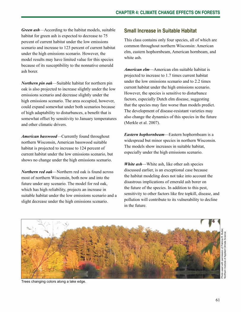
61
CHAPTER 4: CLIMATE CHANGE EFFECTS ON FORESTS
Green ash—According to the habitat models, suitable habitat for green ash is expected to decrease to 75 percent of current habitat under the low emissions scenario and increase to 123 percent of current habitat under the high emissions scenario. However, the model results may have limited value for this species because of its susceptibility to the nonnative emerald ash borer.
Northern pin oak—Suitable habitat for northern pin oak is also projected to increase slightly under the low emissions scenario and decrease slightly under the high emissions scenario. The area occupied, however, could expand somewhat under both scenarios because of high adaptability to disturbances, a benefi t that is somewhat offset by sensitivity to January temperatures and other climatic drivers.
American basswood—Currently found throughout northern Wisconsin, American basswood suitable habitat is projected to increase to 124 percent of current habitat under the low emissions scenario, but shows no change under the high emissions scenario.
Northern red oak—Northern red oak is found across most of northern Wisconsin, both now and into the future under any scenario. The model for red oak, which has high reliability, projects an increase in suitable habitat under the low emissions scenario and a slight decrease under the high emissions scenario.
Small Increase in Suitable Habitat
This class contains only four species, all of which are common throughout northern Wisconsin: American elm, eastern hophornbeam, American hornbeam, and white ash.
American elm—American elm suitable habitat is projected to increase to 1.7 times current habitat under the low emissions scenario and to 2.2 times current habitat under the high emissions scenario. However, the species is sensitive to disturbance factors, especially Dutch elm disease, suggesting that the species may fare worse than models predict. The development of disease-resistant varieties may also change the dynamics of this species in the future (Merkle et al. 2007).
Eastern hophornbeam—Eastern hophornbeam is a widespread but minor species in northern Wisconsin. The models show increases in suitable habitat, especially under the high emissions scenario.
White ash—White ash, like other ash species discussed earlier, is an exceptional case because the habitat modeling does not take into account the disastrous implications of emerald ash borer on the future of the species. In addition to this pest, sensitivity to other factors like fi re topkill, disease, and pollution will contribute to its vulnerability to decline in the future.
Trees changing colors along a lake edge.
Pho
to u
sed
with
per
mis
sion
of P
atric
ia R
. But
ler,
Nor
ther
n In
stitu
te o
f App
lied
Clim
ate
Sci
ence
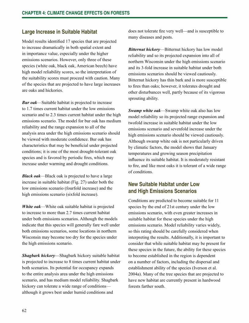
62
CHAPTER 4: CLIMATE CHANGE EFFECTS ON FORESTS
Large Increase in Suitable Habitat
Model results identifi ed 17 species that are projected to increase dramatically in both spatial extent and in importance value, especially under the higher emissions scenarios. However, only three of these species (white oak, black oak, American beech) have high model reliability scores, so the interpretation of the suitability scores must proceed with caution. Many of the species that are projected to have large increases are oaks and hickories.
Bur oak—Suitable habitat is projected to increase to 1.7 times current habitat under the low emissions scenario and to 2.3 times current habitat under the high emissions scenario. The model for bur oak has medium reliability and the range expansion to all of the analysis area under the high emissions scenario should be viewed with moderate confi dence. Bur oak has characteristics that may be benefi cial under projected conditions; it is one of the most drought-tolerant oak species and is favored by periodic fi res, which may increase under warming and drought conditions.
Black oak—Black oak is projected to have a large increase in suitable habitat (Fig. 27) under both the low emissions scenario (fourfold increase) and the high emissions scenario (sixfold increase).
White oak—White oak suitable habitat is projected to increase to more than 2.7 times current habitat under both emissions scenarios. Although the models indicate that this species will generally fare well under both emissions scenarios, some locations in northern Wisconsin may become too dry for the species under the high emissions scenario.
Shagbark hickory—Shagbark hickory suitable habitat is projected to increase to 8 times current habitat under both scenarios. Its potential for occupancy expands to the entire analysis area under the high emissions scenario, and has medium model reliability. Shagbark hickory can tolerate a wide range of conditions—although it grows best under humid conditions and
does not tolerate fi re very well—and is susceptible to many diseases and pests.
Bitternut hickory—Bitternut hickory has low model reliability and so its projected expansion into all of northern Wisconsin under the high emissions scenario and its 3-fold increase in suitable habitat under both emissions scenarios should be viewed cautiously. Bitternut hickory has thin bark and is more susceptible to fi res than oaks; however, it tolerates drought and other disturbances well, partly because of its vigorous sprouting ability.
Swamp white oak—Swamp white oak also has low model reliability so its projected range expansion and twofold increase in suitable habitat under the low emissions scenario and sevenfold increase under the high emissions scenario should be viewed cautiously. Although swamp white oak is not particularly driven by climatic factors, the model shows that January temperatures and growing season precipitation infl uence its suitable habitat. It is moderately resistant to fi re, and like most oaks it is tolerant of a wide range of conditions.
New Suitable Habitat under Low and High Emissions Scenarios
Conditions are predicted to become suitable for 11 species by the end of 21st century under the low emissions scenario, with even greater increases in suitable habitat for these species under the high emissions scenario. Model reliability varies widely, so this rating should be carefully considered when interpreting the results. Additionally, it is important to consider that while suitable habitat may be present for these species in the future, the ability for these species to become established in the region is dependent on a number of factors, including the dispersal and establishment ability of the species (Iverson et al. 2004a). Many of the tree species that are projected to have new habitat are currently present in hardwood forests farther south.
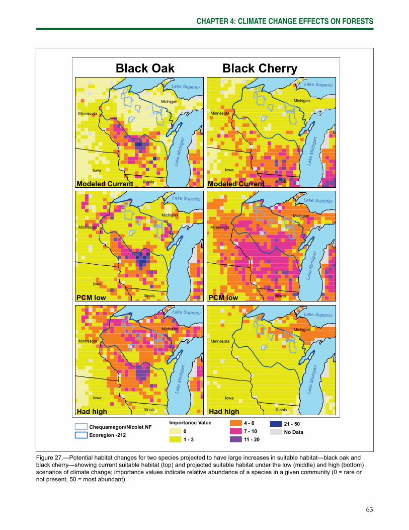
63
CHAPTER 4: CLIMATE CHANGE EFFECTS ON FORESTS
Lake
Mic
higa
n
Lake Superior
Iowa
Minnesota
Michigan
Illinois
Black Oak Black Cherry
Lake Superior
Iowa
Minnesota
Michigan
Illinois
Lake
Mic
higa
n
Lake Superior
Minnesota
Michigan
Illinois
Lake
Mic
higa
n
Lake Superior
Iowa
Minnesota
Michigan
Illinois
Lake
Mic
higa
nLake Superior
Iowa
Minnesota
Michigan
Illinois
Modeled Current
PCM low
Had high
Lake
Mic
higa
n
Lake Superior
Iowa
Minnesota
Michigan
Illinois
PCM low
Had high
Modeled Current
Chequamegon/Nicolet NFEcoregion -212
Importance Value01 - 3
4 - 67 - 1011 - 20
21 - 50No Data
Figure 27.—Potential habitat changes for two species projected to have large increases in suitable habitat—black oak and black cherry—showing current suitable habitat (top) and projected suitable habitat under the low (middle) and high (bottom) scenarios of climate change; importance values indicate relative abundance of a species in a given community (0 = rare or not present, 50 = most abundant).
64
CHAPTER 4: CLIMATE CHANGE EFFECTS ON FORESTS
Pignut hickory—Substantial amounts of suitable habitat for pignut hickory may be present in northern Wisconsin by the end of the century, especially under the high emissions scenario. Model reliability for pignut hickory is high, and the species now exists in temperature and precipitation regimes similar to those projected for the analysis area under both emissions scenarios, especially the low emissions scenario.
Mockernut hickory—Mockernut hickory shows potential expansion of habitat into the region, with substantial amounts of suitable habitat appearing under the high emissions scenario and less under the low emissions scenario. Because the species shows very positive response to disturbances—particularly drought, wind, and disease— it may do better than modeled.
Flowering dogwood—Flowering dogwood habitat is modeled, with moderate reliability, to behave similarly to hickory species (above) in area and habitat quality. Although the species is not expected to have large increases in importance value, suitable habit is projected to expand to include 70 percent of the region under the high emissions scenario and 15 percent under the low emissions scenario.
Yellow-poplar—A large increase in the extent of suitable habitat is projected under the high emissions scenario (to about 40 percent of northern Wisconsin) but only a very small increase is projected under the low emissions scenario (Fig. 28).
Sassafras—Sassafras is modeled to have suitable habitat increase to occupy almost 80 percent of northern Wisconsin under the high emissions scenario and 30 percent under the low emissions scenario.
New Suitable Habitat under the High Emissions Scenario Only
This group of 16 species is characterized by little or no current occupancy in northern Wisconsin, but the models indicate that suitable habitat could appear by the end of the century under the high emissions scenario.
Blackgum—Blackgum shows some range expansion into roughly 20 percent of northern Wisconsin under the high emissions scenario, but with a very low level of suitable habitat within that area. The model has high reliability, but the species could do even better than modeled given its positive response to disturbance and biological factors.
Blackjack oak—Habitat for blackjack oak is projected to appear throughout most of northern Wisconsin under the high emissions scenario only. Although this model has medium reliability, it should be treated with caution since the species’ current range is more than 340 miles (550 kilometers) to the south.
Sycamore—Suitable habitat is projected to increase greatly under the high emissions scenario (to 80 percent of northern Wisconsin) but to only a minor extent under the low emissions scenario. The species’ current range boundary is approximately 110 miles (180 kilometers) from the nearest part of the analysis area.
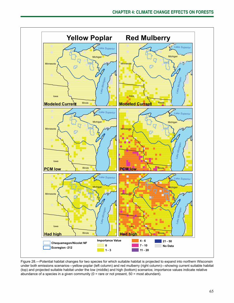
65
CHAPTER 4: CLIMATE CHANGE EFFECTS ON FORESTS
Chequamegon/Nicolet NFEcoregion -212
Importance Value01 - 3
4 - 67 - 1011 - 20
21 - 50No Data
Lake
Mic
higa
n
Lake Superior
Iowa
Minnesota
Michigan
Illinois
Yellow Poplar Red Mulberry
Lake Superior
Iowa
Minnesota
Michigan
Illinois
Lake
Mic
higa
n
Lake Superior
Minnesota
Michigan
Illinois
Lake
Mic
higa
n
Lake Superior
Iowa
Minnesota
Michigan
Illinois
Lake
Mic
higa
nLake Superior
Iowa
Minnesota
Michigan
Illinois
Modeled Current
PCM low
Had high
Lake
Mic
higa
n
Lake Superior
Iowa
Minnesota
Michigan
Illinois
PCM low
Had high
Modeled Current
Figure 28.—Potential habitat changes for two species for which suitable habitat is projected to expand into northern Wisconsin under both emissions scenarios—yellow-poplar (left column) and red mulberry (right column)—showing current suitable habitat (top) and projected suitable habitat under the low (middle) and high (bottom) scenarios; importance values indicate relative abundance of a species in a given community (0 = rare or not present, 50 = most abundant).
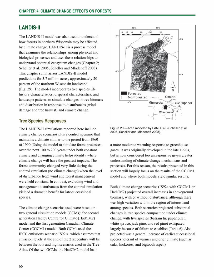
66
CHAPTER 4: CLIMATE CHANGE EFFECTS ON FORESTS
LANDIS-II
The LANDIS-II model was also used to understand how forests in northern Wisconsin may be affected by climate change. LANDIS-II is a process model that examines the relationships among physical and biological processes and uses these relationships to understand potential ecosystem changes (Chapter 2;Scheller et al. 2005, Scheller and Mladenoff 2008). This chapter summarizes LANDIS-II model predictions for 3.7 million acres, approximately 20 percent of the northern Wisconsin landscape (Fig. 29). The model incorporates tree species life history characteristics, dispersal characteristics, and landscape patterns to simulate changes in tree biomass and distribution in response to disturbances (wind damage and tree harvest) and climate change.
Tree Species Responses
The LANDIS-II simulations reported here include climate change scenarios plus a control scenario that maintains a climate similar to the period from 1960 to 1990. Using the model to simulate forest processes over the next 100 to 200 years under both constant climate and changing climate helps identify where climate change will have the greatest impacts. The forest community changed very little during the control simulation (no climate change) when the level of disturbance from wind and forest management were held constant. In contrast, excluding wind and management disturbances from the control simulation yielded a dramatic benefi t for late-successional species.
The climate change scenarios used were based on two general circulation models (GCMs): the second generation Hadley Centre for Climate (HadCM2) model and the fi rst generation Canadian Climate Center (CGCM1) model. Both GCMs used the IPCC emissions scenario IS92A, which assumes that emission levels at the end of the 21st century will be between the low and high scenarios used in the Tree Atlas. Of the two GCMs, the HadCM2 model has
Figure 29.—Area modeled by LANDIS-II (Scheller et al. 2005, Scheller and Mladenoff 2008).
a more moderate warming response to greenhouse gases. It was originally developed in the late 1990s, but is now considered too unresponsive given greater understanding of climate change mechanisms and processes. For this reason, the results presented in this section will largely focus on the results of the CGCM1 model and where both models yield similar results.
Both climate change scenarios (IS92a with CGCM1 or HadCM2) projected overall increases in aboveground biomass, with or without disturbance, although there was high variation within the region of interest and among species. Both scenarios projected substantial changes in tree species composition under climate change, with fi ve species (balsam fi r, paper birch, white spruce, jack pine, and red pine) extirpated largely because of failure to establish (Table 6). Also projected was a general increase of earlier successional species tolerant of warmer and drier climate (such as oaks, hickories, and bigtooth aspen).
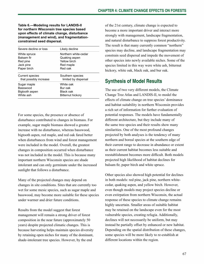
67
CHAPTER 4: CLIMATE CHANGE EFFECTS ON FORESTS
For some species, the presence or absence of disturbance contributed to changes in biomass. For example, sugar maple biomass showed a greater increase with no disturbance, whereas basswood, bigtooth aspen, red maple, and red oak fared better when disturbances from wind and forest management were included in the model. Overall, the greatest changes in composition occurred when disturbance was not included in the model. This is because many important northern Wisconsin species are shade intolerant and can only germinate under the increased sunlight that follows a disturbance.
Many of the projected changes may depend on changes in site conditions. Sites that are currently too wet for some mesic species, such as sugar maple and basswood, may become more suitable for these species under warmer and drier future conditions.
Results from the model suggest that forest management will remain a strong driver of forest composition in the near future (approximately 50 years) despite projected climatic changes. This is because harvesting helps maintain species diversity by retaining open niches for many of the dominant, shade-intolerant tree species. However, by the end
of the 21st century, climate change is expected to become a more important driver and interact more strongly with management, landscape fragmentation, and natural disturbance to suppress forest productivity. The result is that many currently common “northern” species may decline, and landscape fragmentation may constrain seed dispersal and impede the movement of other species into newly available niches. Some of the species limited in this way were white ash, bitternut hickory, white oak, black oak, and bur oak.
Synthesis of Model Results
The use of two very different models, the Climate Change Tree Atlas and LANDIS-II, to model the effects of climate change on tree species’ dominance and habitat suitability in northern Wisconsin provides a rich set of information for further evaluation of potential responses. The models have fundamentally different architecture, but they include many of the same tree species and their results show many similarities. One of the most profound changes projected by both analyses is the tendency of many northern and boreal species at the southern edge of their current range to decrease in abundance or extent as their current habitat becomes less suitable and reestablishment becomes more diffi cult. Both models projected high likelihood of habitat declines for balsam fi r, paper birch and white spruce.
Other species also showed high potential for declines in both models: red pine, jack pine, northern white-cedar, quaking aspen, and yellow birch. However, even though models may project species decline or even extirpation from northern Wisconsin, the actual response of these species to climate change remains highly uncertain. Smaller areas of suitable habitat may be retained on the landscape even for the most vulnerable species, creating refugia. Additionally, declines will not necessarily be uniform, but may instead be partially offset by enhanced or new habitat. Depending on the spatial distribution of these changes, some species will be more likely to re-establish at different locations within the region.
Table 6.—Modeling results for LANDIS-II for northern Wisconsin tree species based upon effects of climate change, disturbance (management and wind), and fragmentation-constrained seed dispersal.
Severe decline or loss Likely decline
White spruce Northern white-cedarBalsam fi r Quaking aspenRed pine Yellow birchJack pine Red maplePaper birch Red oak
Current species Southern species that possibly increase limited by dispersal
Sugar maple White oakBasswood Bur oakBigtooth aspen Black oakWhite ash Bitternut hickory
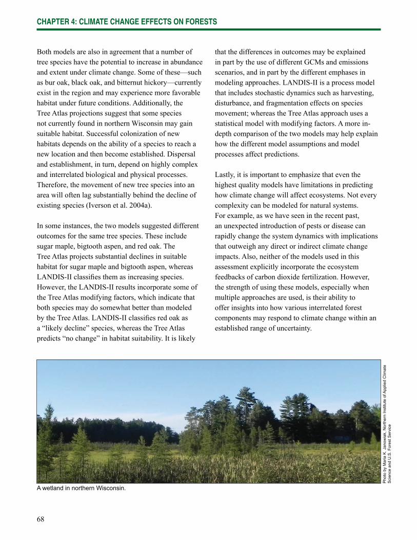
68
CHAPTER 4: CLIMATE CHANGE EFFECTS ON FORESTS
Both models are also in agreement that a number of tree species have the potential to increase in abundance and extent under climate change. Some of these—such as bur oak, black oak, and bitternut hickory—currently exist in the region and may experience more favorable habitat under future conditions. Additionally, the Tree Atlas projections suggest that some species not currently found in northern Wisconsin may gain suitable habitat. Successful colonization of new habitats depends on the ability of a species to reach a new location and then become established. Dispersal and establishment, in turn, depend on highly complex and interrelated biological and physical processes. Therefore, the movement of new tree species into an area will often lag substantially behind the decline of existing species (Iverson et al. 2004a).
In some instances, the two models suggested different outcomes for the same tree species. These include sugar maple, bigtooth aspen, and red oak. The Tree Atlas projects substantial declines in suitable habitat for sugar maple and bigtooth aspen, whereas LANDIS-II classifi es them as increasing species. However, the LANDIS-II results incorporate some of the Tree Atlas modifying factors, which indicate that both species may do somewhat better than modeled by the Tree Atlas. LANDIS-II classifi es red oak as a “likely decline” species, whereas the Tree Atlas predicts “no change” in habitat suitability. It is likely
that the differences in outcomes may be explained in part by the use of different GCMs and emissions scenarios, and in part by the different emphases in modeling approaches. LANDIS-II is a process model that includes stochastic dynamics such as harvesting, disturbance, and fragmentation effects on species movement; whereas the Tree Atlas approach uses a statistical model with modifying factors. A more in-depth comparison of the two models may help explain how the different model assumptions and model processes affect predictions.
Lastly, it is important to emphasize that even the highest quality models have limitations in predicting how climate change will affect ecosystems. Not every complexity can be modeled for natural systems. For example, as we have seen in the recent past, an unexpected introduction of pests or disease can rapidly change the system dynamics with implications that outweigh any direct or indirect climate change impacts. Also, neither of the models used in this assessment explicitly incorporate the ecosystem feedbacks of carbon dioxide fertilization. However, the strength of using these models, especially when multiple approaches are used, is their ability to offer insights into how various interrelated forest components may respond to climate change within an established range of uncertainty.
A wetland in northern Wisconsin.
Pho
to b
y M
aria
K. J
anow
iak,
Nor
ther
n In
stitu
te o
f App
lied
Clim
ate
Sci
ence
and
U.S
. For
est S
ervi
ce
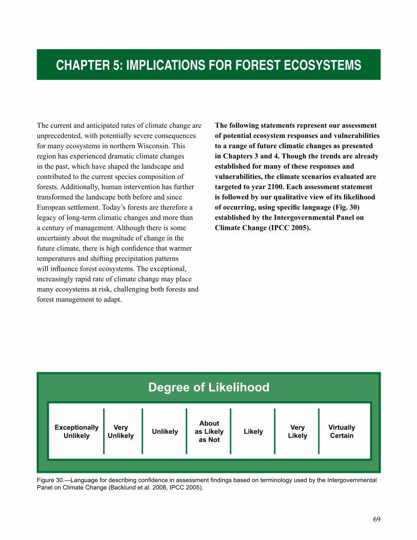
69
CHAPTER 5: IMPLICATIONS FOR FOREST ECOSYSTEMS
The current and anticipated rates of climate change are unprecedented, with potentially severe consequences for many ecosystems in northern Wisconsin. This region has experienced dramatic climate changes in the past, which have shaped the landscape and contributed to the current species composition of forests. Additionally, human intervention has further transformed the landscape both before and since European settlement. Today’s forests are therefore a legacy of long-term climatic changes and more than a century of management. Although there is some uncertainty about the magnitude of change in the future climate, there is high confi dence that warmer temperatures and shifting precipitation patterns will infl uence forest ecosystems. The exceptional, increasingly rapid rate of climate change may place many ecosystems at risk, challenging both forests and forest management to adapt.
The following statements represent our assessment of potential ecosystem responses and vulnerabilities to a range of future climatic changes as presented in Chapters 3 and 4. Though the trends are already established for many of these responses and vulnerabilities, the climate scenarios evaluated are targeted to year 2100. Each assessment statement is followed by our qualitative view of its likelihood of occurring, using specifi c language (Fig. 30) established by the Intergovernmental Panel on Climate Change (IPCC 2005).
Figure 30.—Language for describing confi dence in assessment fi ndings based on terminology used by the Intergovernmental Panel on Climate Change (Backlund et al. 2008, IPCC 2005).
Degree of Likelihood
Exceptionally Unlikely
Very Unlikely Unlikely
Aboutas Likely
as NotLikely Very
LikelyVirtually Certain
70
CHAPTER 5: IMPLICATIONS FOR FOREST ECOSYSTEMS
Shifting Stressors
Climate change may relieve some stressors, while exacerbating others. Warmer temperatures and shifting precipitation patterns are expected to strongly infl uence ecosystem drivers.
Temperatures will increase (virtually certain) Annual increases in temperature represent the broadest possible stressor, strongly infl uencing other stressors and ecosystem responses. Even the most conservative models and scenarios project an increase in average temperature for northern Wisconsin (IPCC 2007, WICCI 2009). These increases are projected to be greatest in the winter, with daily lows more affected than daily highs (Chapter 3). Warmer annual averages have already been shown to affect the structure and function of ecosystems by directly or indirectly altering hydrology, soil conditions, and nutrient cycling. These changes further affect species phenology, range and distribution, community composition, and complex ecosystem dynamics (Huntington et al. 2009, Walther et al. 2002). Warmer winter temperatures and longer growing seasons could benefi t some species, but these changes may not synchronize with other ecosystem responses and climate variables and may ultimately result in a net negative effect. For example, day length will not change, so the ultimate effect on various species is not clear. Summer temperatures are also expected to continue rising, leading to reduced water availability and increased drought stress and fi re risk, especially in late summer (Huntington 2008).
Growing seasons will get longer (virtually certain) There is already evidence of growing seasons lengthening throughout much of Wisconsin over the last several decades, and this trend is virtually certain to continue. Temperature increases and longer growing seasons will affect ecosystem and physiological processes (Bradley et al. 1999, Campbell et al. 2009). Earlier springs and longer growing seasons
will likely translate into shifts in the phenology of plant species that rely on temperature as a cue for the timing of reproductive maturation and other developmental processes (Schwartz et al. 2006a, Walther et al. 2002). Shifts in phenology have already been observed for a number of temperate species and can be linked to a warming climate (Bradley et al. 1999, Richardson et al. 2006, Schwartz et al. 2006a). Longer growing seasons could also result in greater growth and productivity of vegetation (Drake et al. 1997). However, productivity will largely depend on the amount of moisture and nutrients that are available to plants throughout the growing season. Although, carbon dioxide increases in the atmosphere have been shown to reduce the rate of water lost from plants through evapotranspiration (Gedney et al. 2006), there will likely be a net increase in evapotranspiration in response to higher temperatures and a longer growing season (Huntington 2008, IPCC 2007). A longer growing season is thus likely to create greater water demand, which will cause plant stress if the demand is not synchronized with adequate water supply.
The nature and timing of precipitation will change (virtually certain)It is virtually certain that future precipitation patterns in northern Wisconsin will be substantially different from today, but projections of precipitation differ considerably on the seasonal distribution and magnitude of these changes (IPCC 2007, WICCI 2009). Many of these differences arise because certain fundamental components of climate in northern Wisconsin are inherently diffi cult to model: lake-effect snow, changes in snow frequency and amount, and frequency of events such as severe summer thunderstorms. Some of this uncertainty will be resolved with better coupling of land-water-atmosphere components in medium-scale models, but there will always be annual variation due to the stochastic nature of these events (NRC 2008). The projected overall increase in annual precipitation in northern Wisconsin includes a net increase in some seasons, and a net decrease in others. Most models
71
CHAPTER 5: IMPLICATIONS FOR FOREST ECOSYSTEMS
project that northern Wisconsin will experience an increase in precipitation in the late winter or early spring, but there is a trend toward reduced precipitation in the late summer and early autumn (Hayhoe et al. 2007, Plummer et al. 2006, WICCI 2009). These changes can have considerable effects on hydrology and groundwater recharge, and could lead to increased drought stress in the late summer (Huntington et al. 2009). Signifi cant increases in lake-effect snow during the 20th century have been detected in the Great Lakes region, and those increases may be the result of warmer surface waters and decreased ice cover on the Great Lakes (Burnett et al. 2003). Continued temperature increases in late winter will likely cause more winter precipitation to fall as rain. However, it is still unclear exactly to what extent air temperature, weather patterns, and other factors will interact to change precipitation events from snow to rain in the coming decades.
Soil moisture patterns will change (virtually certain), with drier soil conditions later in the growing season (likely)The reduction of late summer rain suggested by several models, coupled with increases in evapotranspiration from increased temperatures, will likely lead to decreases in soil moisture later in the growing season (Dai et al. 2004). Even if there are increases in precipitation in the summer, as a few models suggest, increases in evapotranspiration will likely lead to lower soil water availability (Hayhoe et al. 2007, Huntington et al. 2004, Ollinger et al. 2008). This may interact with a longer growing season to exacerbate overall stress on the system. In addition, a shift from snow to rain in the winter could cause more winter precipitation to runoff rather than be stored in the snowpack, resulting in less water stored in the soil, and contributing to drier soils later in the summer (Huntington et al. 2009). Drier soils, especially forest fl oors, may also increase susceptibility to wildfi res (Dale et al. 2001). Just as dry soils may be problematic in warm temperatures, wet soils may present a problem if exposed to freezing temperatures. Soils covered by deep snowpack early in the season can be
insulated from severely cold temperatures and remain unfrozen throughout the winter (Decker et al. 2003). If higher winter temperatures reduce the snowpack, the resulting soil freezing could be damaging to fi ne roots of trees, such as sugar maple, that are vulnerable to rapid freeze-thaw changes (Mohan et al. 2009). Increases in the frequency and extent of soil frost could also infl uence soil water movement and reduce groundwater recharge, also potentially increasing surface runoff (Hardy et al. 2001, Zhao and Gray 1999). Changes in soil moisture patterns will vary widely by season and landscape position, but increases in the length and severity of late summer drought will likely have the most widespread effects.
The frequency, size, and severity of natural disturbances will change across the landscape (very likely)Climate change may accelerate the frequency or increase the severity of disturbances, such as drought, catastrophic winds, ice storms, rainstorms, wildfi res, and fl oods (Campbell et al. 2009, Dale et al. 2001, Dukes et al. 2009, Hanson and Weltzin 2000, Mohan et al. 2009, Peterson 2000), and indeed, evidence continues to mount that disturbance events are increasing in frequency (e.g., Westerling 2006 ) and intensity (e.g., Min et al. 2011). Changes in these various disturbance regimes, with their ability to fundamentally alter ecosystems, may have the most obvious and even drastic effects on northern Wisconsin forests. Some of these disturbances may also interact to increase system susceptibility to other disturbances.
Increased annual temperatures can increase the incidence of drought and tree mortality, potentially increasing the incidence of downed and dead wood and contributing to increased frequency, extent, and severity of wildfi res (Huntington et al. 2009). In one study of boreal forests, the number of acres burned was estimated to double by the end of the 21st century (Flannigan et al. 2009). With fi res occurring more frequently, attempts to control wildfi res will likely become less successful (Flannigan et al. 2009).
72
CHAPTER 5: IMPLICATIONS FOR FOREST ECOSYSTEMS
In areas where fi re is rare, wind may be the most infl uential disturbance type in forests and may increase in severity and occurrence as the atmospheric conditions leading to high winds become more common (Berz 1993, Peterson 2000) and return intervals for severe wind events shorten (Frelich and Reich 2010). Wind damage can shift a system into smaller tree size-class distributions as larger trees suffer more bole breakage, leaving smaller trees as survivors (Peterson 2000). Succession may be set back if sprouts of damaged trees reclaim the canopy, or altered altogether if understory species shift the composition toward late seral species (Peterson 2000).
Ice storms could also increase in frequency with slightly warmer temperatures, causing precipitation to fall as freezing rain instead of snow (NRC 2008). More winter precipitation could further increase the frequency of ice storms. Ice damage can range from light to fatal, depending on the amount and area covered and on stand history, composition, and structure (Dale et al. 2001, Rhoads et al. 2002). Increased frequency and intensity of rainstorms will also increase the risk of fl ooding or erosion in many areas.
Pests and diseases will increase or become more severe (very likely)The combination of increased stress on native species and longer grower seasons can benefi t nonnative and invasive fl ora and fauna. Warming tends to increase the rate of insect development, allowing some pests to complete a second lifecycle in a single growing season (Ayres and Lomabardo 2000, Dukes et al. 2009). When these accelerated life cycles are combined with drought stress, pests can hasten changes in ecosystem composition (Weltzin et al. 2003, Williamson 1999).
The spatial extent of pest damage may also increase. Some pests and diseases that are currently moderated by very cold winter temperatures may better survive warmer winters, increasing their population and expanding their range (Dukes et al. 2009, Karl et
al. 2009). For example, hemlock wooly adelgid is currently limited in its northern expansion by its sensitivity to low winter temperatures and could expand further north as temperatures increase (Paradis et al. 2008). Emerald ash borer’s range in the United States is not known to be limited by current temperatures, but a longer growing season could increase the rate of reproduction and the rate of host mortality if larvae are active later into autumn (Poland and McCullough 2006). Pathogens such as Diplodia pinea, found in red pine, may also become problematic. Water stress may become more frequent and severe in red pine as habitat suitability shifts, resulting in more frequent infections, with consequent loss of productivity or even mortality (Munck et al. 2009, Peterson 1997, Stanosz et al. 2001).
Nonnative invasive plants would also experience changes in distribution and habitat suitability (Sher and Hyatt 1999), but many of these plants are already particularly adept at competing for resources and establishing after disturbances. With increases in forest stress and disturbances, invasives may exacerbate climate impacts on community composition, potentially even creating monocultures of non-desirable species (Sher and Hyatt 1999, Weltzin et al. 2003).
Ecosystem Response to Shifting Stressors
Shifts in stressors will likely lead to changes in forest community composition and ecosystem function. These changes may not be experienced similarly across northern Wisconsin, but instead will impact individual forest types and locations differently as a function of site conditions, species compositions, and management histories (Table 7).
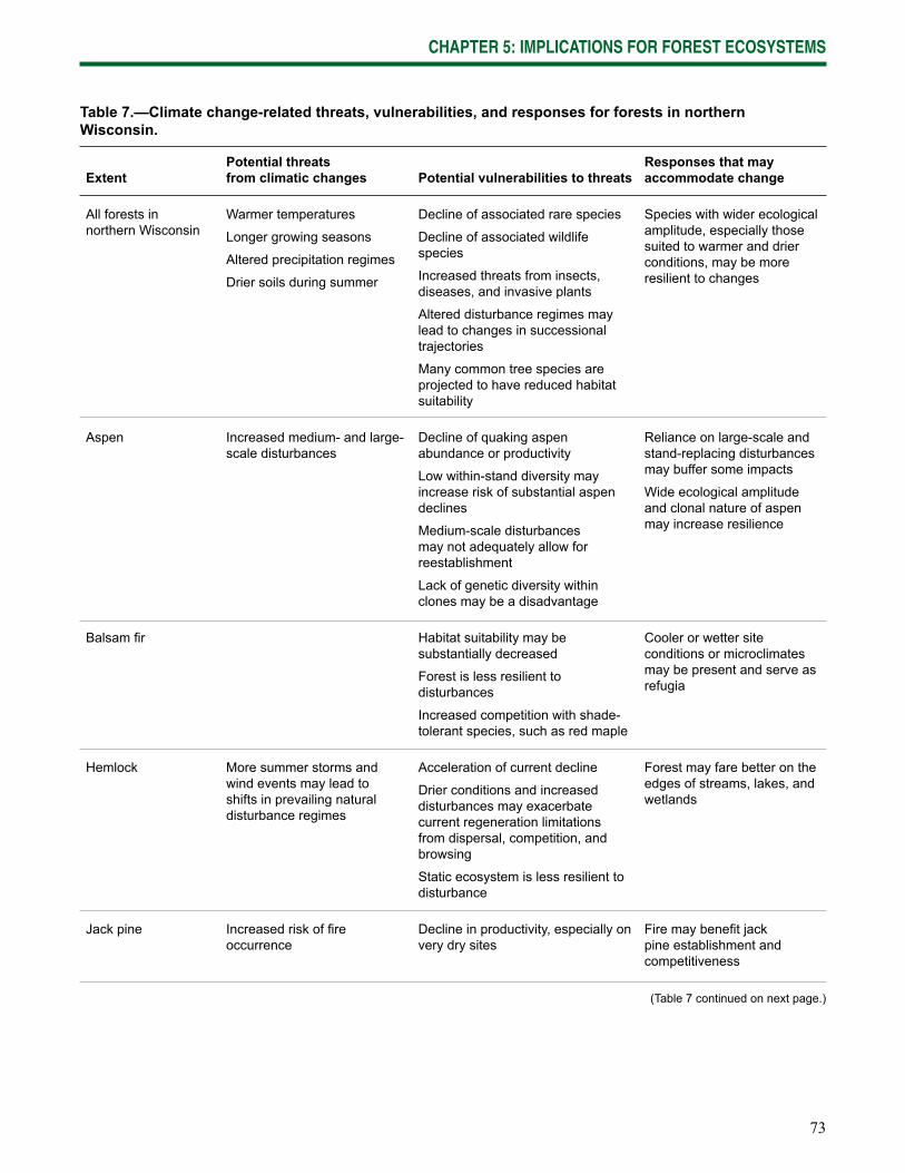
73
CHAPTER 5: IMPLICATIONS FOR FOREST ECOSYSTEMS
ExtentPotential threats from climatic changes Potential vulnerabilities to threats
Responses that may accommodate change
All forests in northern Wisconsin
Warmer temperatures
Longer growing seasons
Altered precipitation regimes
Drier soils during summer
Decline of associated rare species
Decline of associated wildlife species
Increased threats from insects, diseases, and invasive plants
Altered disturbance regimes may lead to changes in successional trajectories
Many common tree species are projected to have reduced habitat suitability
Species with wider ecological amplitude, especially those suited to warmer and drier conditions, may be more resilient to changes
Aspen Increased medium- and large-scale disturbances
Decline of quaking aspen abundance or productivity
Low within-stand diversity may increase risk of substantial aspen declines
Medium-scale disturbances may not adequately allow for reestablishment
Lack of genetic diversity within clones may be a disadvantage
Reliance on large-scale and stand-replacing disturbances may buffer some impacts
Wide ecological amplitude and clonal nature of aspen may increase resilience
Balsam fi r Habitat suitability may be substantially decreased
Forest is less resilient to disturbances
Increased competition with shade- tolerant species, such as red maple
Cooler or wetter site conditions or microclimates may be present and serve as refugia
Hemlock More summer storms and wind events may lead to shifts in prevailing natural disturbance regimes
Acceleration of current decline
Drier conditions and increased disturbances may exacerbate current regeneration limitations from dispersal, competition, and browsing
Static ecosystem is less resilient to disturbance
Forest may fare better on the edges of streams, lakes, and wetlands
Jack pine Increased risk of fi re occurrence
Decline in productivity, especially on very dry sites
Fire may benefi t jack pine establishment and competitiveness
Table 7.—Climate change-related threats, vulnerabilities, and responses for forests in northern Wisconsin.
(Table 7 continued on next page.)

74
CHAPTER 5: IMPLICATIONS FOR FOREST ECOSYSTEMS
ExtentPotential threats from climatic changes Potential vulnerabilities to threats
Responses that may accommodate change
Lowland conifer Altered hydrology and precipitation patterns may lead to reduced duration of soil saturation or ponding
Increased risk of fi re occurrence in dried organic soils
Habitat suitability may be substantially decreased
Reduced soil moisture or saturation may cause declines in hydrophytic tree species
Static ecosystem is less resilient to disturbance
Non-peatland sites may fare better
Cooler or wetter site conditions or microclimates may be present and serve as refugia
Lowland hardwood Altered hydrology and precipitation patterns may lead to reduced duration of soil saturation or ponding
Black ash habitat suitability may be substantially decreased
Low within-stand diversity may increase risk if black ash declines substantially
Drier conditions may lead to increased competition from other tree and plant species
Emerald ash borer may interact with other stressors to cause widespread mortality
Decline of black ash may be buffered where other species are present, such as red maple
Cooler or wetter site conditions or microclimates may be present and serve as refugia
Northern hardwood More summer storms and wind events may alter prevailing natural disturbance regimes
Increased root damage from altered freeze-thaw cycles
Decline of sugar maple productivity, especially on drier sites
Increased disturbances may accelerate current decline of eastern hemlock and yellow birch
Drying of ephemeral ponds may increase stress on associated species
Decline of some species may be buffered where tree species composition is diverse
Oak Decline in productivity, especially on very dry sites
Warmer and drier conditions may favor oak species on a variety of sites
Oak species not currently present may expand into new areas, but extent is limited by dispersal, winter temperatures, competition, and browsing
Paper Birch Increased fi re and wind disturbance
Increased disturbances may accelerate current decline
Wind or other medium-scale disturbances may not adequately allow for reestablishment
Fire may create conditions needed for paper birch establishment
(Table 7 continued on next page.)
Table 7 (continued).—Climate change-related threats, vulnerabilities, and responses for forests in northern Wisconsin.
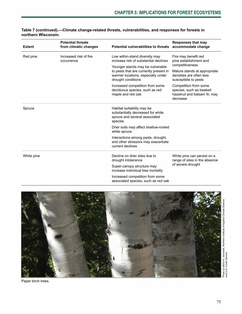
75
CHAPTER 5: IMPLICATIONS FOR FOREST ECOSYSTEMS
ExtentPotential threats from climatic changes Potential vulnerabilities to threats
Responses that may accommodate change
Red pine Increased risk of fi re occurrence
Low within-stand diversity may increase risk of substantial declines
Younger stands may be vulnerable to pests that are currently present in warmer locations, especially under drought conditions
Increased competition from some deciduous species, such as red maple and red oak
Fire may benefi t red pine establishment and competitiveness
Mature stands at appropriate densities are often less susceptible to pests
Competition from some species, such as beaked hazelnut and balsam fi r, may decrease
Spruce Habitat suitability may be substantially decreased for white spruce and several associated species
Drier soils may affect shallow-rooted white spruce
Interactions among pests, drought, and other stressors may exacerbate current declines
White pine Decline on drier sites due to drought intolerance
Super-canopy structure may increase individual tree mortality
Increased competition from some associated species, such as red oak
White pine can persist on a range of sites in the absence of severe drought
Paper birch trees.
Pho
to b
y M
aria
K. J
anow
iak,
Nor
ther
n In
stitu
te o
f App
lied
Clim
ate
Sci
ence
an
d U
.S. F
ores
t Ser
vice
Table 7 (continued).—Climate change-related threats, vulnerabilities, and responses for forests in northern Wisconsin.
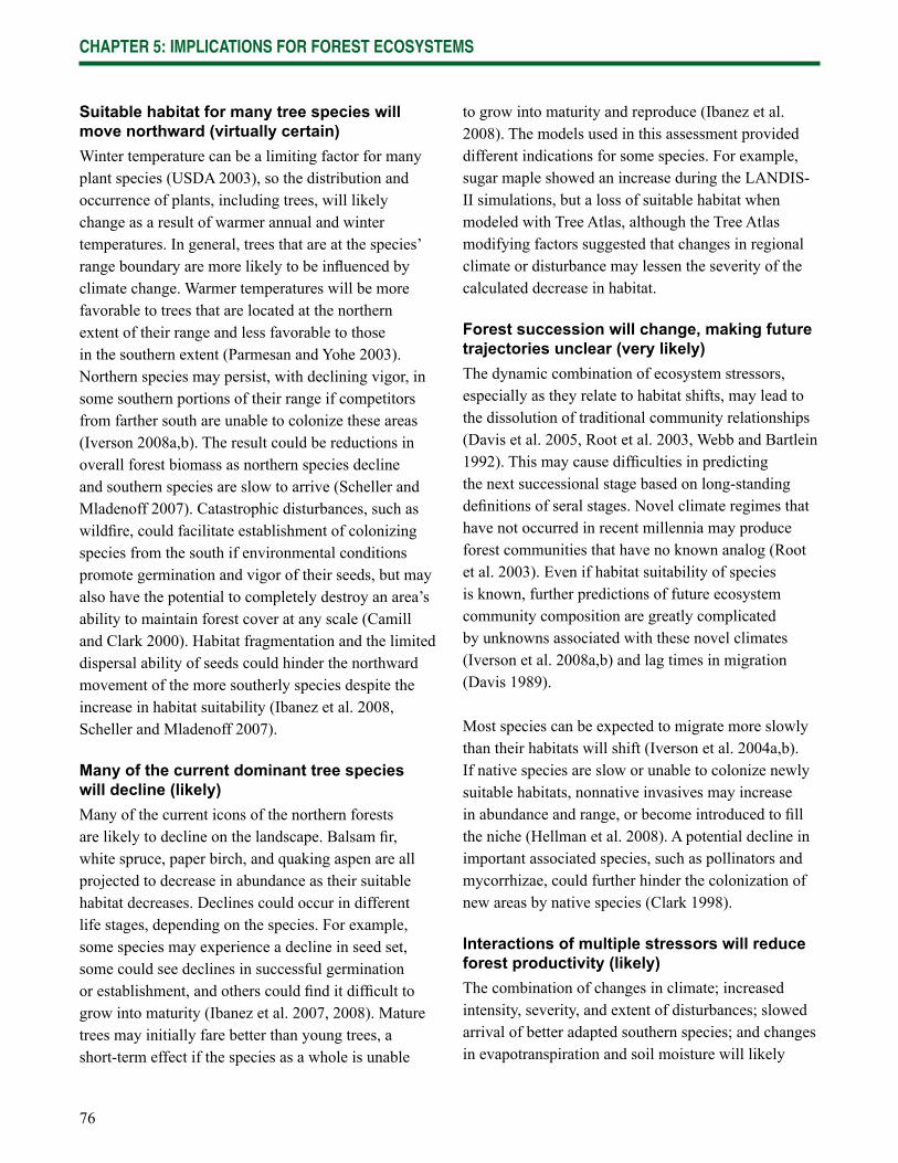
76
CHAPTER 5: IMPLICATIONS FOR FOREST ECOSYSTEMS
Suitable habitat for many tree species will move northward (virtually certain)Winter temperature can be a limiting factor for many plant species (USDA 2003), so the distribution and occurrence of plants, including trees, will likely change as a result of warmer annual and winter temperatures. In general, trees that are at the species’ range boundary are more likely to be infl uenced by climate change. Warmer temperatures will be more favorable to trees that are located at the northern extent of their range and less favorable to those in the southern extent (Parmesan and Yohe 2003). Northern species may persist, with declining vigor, in some southern portions of their range if competitors from farther south are unable to colonize these areas (Iverson 2008a,b). The result could be reductions in overall forest biomass as northern species decline and southern species are slow to arrive (Scheller and Mladenoff 2007). Catastrophic disturbances, such as wildfi re, could facilitate establishment of colonizing species from the south if environmental conditions promote germination and vigor of their seeds, but may also have the potential to completely destroy an area’s ability to maintain forest cover at any scale (Camill and Clark 2000). Habitat fragmentation and the limited dispersal ability of seeds could hinder the northward movement of the more southerly species despite the increase in habitat suitability (Ibanez et al. 2008, Scheller and Mladenoff 2007).
Many of the current dominant tree species will decline (likely)Many of the current icons of the northern forests are likely to decline on the landscape. Balsam fi r, white spruce, paper birch, and quaking aspen are all projected to decrease in abundance as their suitable habitat decreases. Declines could occur in different life stages, depending on the species. For example, some species may experience a decline in seed set, some could see declines in successful germination or establishment, and others could fi nd it diffi cult to grow into maturity (Ibanez et al. 2007, 2008). Mature trees may initially fare better than young trees, a short-term effect if the species as a whole is unable
to grow into maturity and reproduce (Ibanez et al. 2008). The models used in this assessment provided different indications for some species. For example, sugar maple showed an increase during the LANDIS-II simulations, but a loss of suitable habitat when modeled with Tree Atlas, although the Tree Atlas modifying factors suggested that changes in regional climate or disturbance may lessen the severity of the calculated decrease in habitat.
Forest succession will change, making future trajectories unclear (very likely)The dynamic combination of ecosystem stressors, especially as they relate to habitat shifts, may lead to the dissolution of traditional community relationships (Davis et al. 2005, Root et al. 2003, Webb and Bartlein 1992). This may cause diffi culties in predicting the next successional stage based on long-standing defi nitions of seral stages. Novel climate regimes that have not occurred in recent millennia may produce forest communities that have no known analog (Root et al. 2003). Even if habitat suitability of species is known, further predictions of future ecosystem community composition are greatly complicated by unknowns associated with these novel climates (Iverson et al. 2008a,b) and lag times in migration (Davis 1989).
Most species can be expected to migrate more slowly than their habitats will shift (Iverson et al. 2004a,b). If native species are slow or unable to colonize newly suitable habitats, nonnative invasives may increase in abundance and range, or become introduced to fi ll the niche (Hellman et al. 2008). A potential decline in important associated species, such as pollinators and mycorrhizae, could further hinder the colonization of new areas by native species (Clark 1998).
Interactions of multiple stressors will reduce forest productivity (likely)The combination of changes in climate; increased intensity, severity, and extent of disturbances; slowed arrival of better adapted southern species; and changes in evapotranspiration and soil moisture will likely
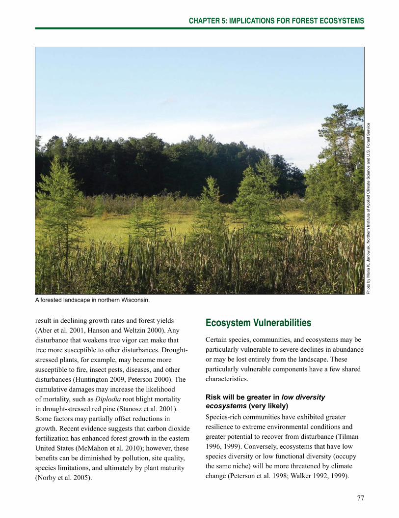
77
CHAPTER 5: IMPLICATIONS FOR FOREST ECOSYSTEMS
result in declining growth rates and forest yields (Aber et al. 2001, Hanson and Weltzin 2000). Any disturbance that weakens tree vigor can make that tree more susceptible to other disturbances. Drought-stressed plants, for example, may become more susceptible to fi re, insect pests, diseases, and other disturbances (Huntington 2009, Peterson 2000). The cumulative damages may increase the likelihood of mortality, such as Diplodia root blight mortality in drought-stressed red pine (Stanosz et al. 2001). Some factors may partially offset reductions in growth. Recent evidence suggests that carbon dioxide fertilization has enhanced forest growth in the eastern United States (McMahon et al. 2010); however, these benefi ts can be diminished by pollution, site quality, species limitations, and ultimately by plant maturity (Norby et al. 2005).
Ecosystem Vulnerabilities
Certain species, communities, and ecosystems may be particularly vulnerable to severe declines in abundance or may be lost entirely from the landscape. These particularly vulnerable components have a few shared characteristics.
Risk will be greater in low diversity ecosystems (very likely)Species-rich communities have exhibited greater resilience to extreme environmental conditions and greater potential to recover from disturbance (Tilman 1996, 1999). Conversely, ecosystems that have low species diversity or low functional diversity (occupy the same niche) will be more threatened by climate change (Peterson et al. 1998; Walker 1992, 1999).
A forested landscape in northern Wisconsin.
Pho
to b
y M
aria
K. J
anow
iak,
Nor
ther
n In
stitu
te o
f App
lied
Clim
ate
Sci
ence
and
U.S
. For
est S
ervi
ce
78
CHAPTER 5: IMPLICATIONS FOR FOREST ECOSYSTEMS
Ecosystems currently dominated almost entirely by a single species may experience severe degradation if that species declines. Within northern hardwood ecosystems, for example, stands dominated by sugar maple may be more vulnerable than those containing larger components of red maple, red oak, basswood, and other associates that offer a wider range of moisture tolerance.
Genetic diversity within species is also critical for the ability of populations to adapt to climate change, because species with high genetic variation are more resilient to disturbance (Reusch et al. 2005). It is unclear, however, how changing climate stressors will affect contemporary plant community genetics. The effects of climate change on tree reproductive processes may result in lower reproductive success and decreases in population size and genetic diversity. Fragmentation and deforestation also increase the potential for inbreeding and reduced genetic diversity (Bawa and Dayanandan 1998). Species with low genetic diversity, especially plantation monocultures, are often intolerant of disturbances and more susceptible to insect outbreaks, exacerbating the vulnerability of those species to climate change (Noss 2001). In natural systems, low genetic diversity may contribute to species- or community-level declines; for plantation species, more intensive management practices may mitigate such effects.
Disturbance will destabilize static ecosystems (very likely)Systems that are less resilient to disturbances may be particularly vulnerable as a wide range of natural disturbances increase, including drought, wind events, fi re, ice storms, and wind storms. For example, lowland hardwood, lowland conifer, northern hardwood, and hemlock forests are not fi re-adapted. They may experience an increase in fi re frequency or severity under drier conditions, making them unable to recover to their previous state (Dale et al. 2001). An increase in fi re could also pave the way for more fi re-adapted species such as jack pine or oak.
Climate change will exacerbate problems for species already in decline (very likely)Model results in this assessment indicate that climate change is projected to reduce habitat suitability for many species that are already experiencing declines. Eastern hemlock and yellow birch are currently declining in northern Wisconsin from natural or human-induced causes (Rooney et al. 2000, Zhu et al. 2000), and recruitment of northern white-cedar is very low (Forester et al. 2008). Historic mid-Holocene declines of eastern hemlock and white spruce have coincided with periods of climate warming and drought in the past, and those declines have been attributed mainly to insect pests (Bhiry and Filion 1996). More recently, logging in the mid-to-late 1800s resulted in slash fi res that destroyed seeds and seedlings, and the drought-sensitive hemlock has been unable to recover in affected areas (Mladenoff et al. 2008). The replacement of hemlock by sugar maple and other hardwoods has further decreased the habitat suitability for establishment of its seedlings; this, combined with deer browsing and periods of drought, has slowed recruitment within hemlock stands to levels that are too low to maintain the cover type (Rooney et al. 2000). Climate change is expected to exacerbate this loss through increases in drought incidence and reductions in summer soil moisture, further reducing seedling and sapling recruitment and the vigor of mature trees (Rooney et al. 2000).
Additionally, intolerance to injury during winter freeze-thaw events is thought to play a signifi cant role in yellow birch decline. Absence of snow cover increases the vulnerability of the shallow roots to freezing and the stem xylem to cavitation. Warmer winters and longer winter thaws may lead to increased damage in yellow birch and result in reduced spring shoot growth (Zhu et al. 2000).
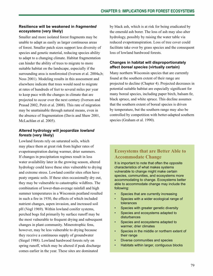
79
CHAPTER 5: IMPLICATIONS FOR FOREST ECOSYSTEMS
Resilience will be weakened in fragmented ecosystems (very likely)Smaller and more isolated forest fragments may be unable to adapt as easily as larger continuous areas of forest. Smaller patch sizes support less diversity of species and genetic material, reducing species ability to adapt to a changing climate. Habitat fragmentation can hinder the ability of trees to migrate to more suitable habitat on the landscape, especially if the surrounding area is nonforested (Iverson et al. 2004a,b; Noss 2001). Modeling results in this assessment and elsewhere indicate that trees would need to migrate at rates of hundreds of feet to several miles per year to keep pace with the changes in climate that are projected to occur over the next century (Iverson and Prasad 2002, Petit et al. 2008). This rate of migration may be unattainable through natural means, even in the absence of fragmentation (Davis and Shaw 2001, McLachlan et al. 2005).
Altered hydrology will jeopardize lowland forests (very likely)Lowland forests rely on saturated soils, which may place them at great risk from higher rates of evapotranspiration during warmer, drier summers. If changes in precipitation regimes result in less water availability later in the growing season, altered hydrology could leave these sites vulnerable to drying and extreme stress. Lowland conifer sites often have peaty organic soils. If these sites occasionally dry out, they may be vulnerable to catastrophic wildfi res. The combination of lower-than-average rainfall and high summer temperatures in a Wisconsin peatland resulted in such a fi re in 1930, the effects of which included nutrient changes, aspen invasion, and increased soil pH (Vogl 1969). Within lowland conifer systems, perched bogs fed primarily by surface runoff may be the most vulnerable to frequent drying and subsequent changes in plant community. Minerotrophic fens, however, may be less vulnerable to drying because they receive a continuous supply of groundwater (Siegel 1988). Lowland hardwood forests rely on spring runoff, which may be altered if peak discharge comes earlier in the year. These sites are dominated
by black ash, which is at risk for being eradicated by the emerald ash borer. The loss of ash may also alter hydrology, possibly by raising the water table via reduced evapotranspiration. Loss of tree cover could facilitate take over by grass species and the consequent loss of lowland hardwood forests.
Changes in habitat will disproportionately affect boreal species (virtually certain) Many northern Wisconsin species that are currently found at the southern extent of their range are projected to decline (Chapter 4). Projected decreases in potential suitable habitat are especially signifi cant for many boreal species, including paper birch, balsam fi r, black spruce, and white spruce. This decline assumes that the southern extent of boreal species is driven by temperature, but the southern range may also be controlled by competition with better-adapted southern species (Graham et al. 1990).
Ecosystems that are Better Able to Accommodate ChangeIt is important to note that often the opposite characteristics of what makes systems vulnerable to change might make certain species, communities, and ecosystems more accommodating to change. Ecosystems better able to accommodate change may include the following: • Species that are currently increasing • Species with a wider ecological range of
tolerances • Species with greater genetic diversity • Species and ecosystems adapted to
disturbances• Species and ecosystems adapted to
warmer, drier climates• Species in the middle or northern extent of
their range• Diverse communities and species• Habitats within larger, contiguous blocks
80
CHAPTER 5: IMPLICATIONS FOR FOREST ECOSYSTEMS
Further reductions in habitat will impact threatened, endangered, and rare species (virtually certain)Species are threatened, endangered, or rare because of specifi c habitat requirements and relative inability to cope with change (Rabinowitz 1981). These same characteristics may make them more vulnerable than other species to changes in climate and subsequent changes in disturbance regimes, soil moisture, pests, and hydrology. Population extinctions of rare and endangered species have already been linked to recent climate change (McLaughlin et al. 2002). Further changes in climate will likely have even greater effects. Because these species are rare, there are often insuffi cient data to model future suitable habitats. For example, there are a number of rare species that are associated with ephemeral ponds, such as the red-shouldered hawk (WDNR 2005). It is hard to predict where, if anywhere, these ponds will exist in the future, and how these species may migrate to new suitable areas.
Ecosystem changes will have signifi cant effects on wildlife (very likely)If forest tree communities change, wildlife species that rely on them may also be vulnerable (Rodenhouse et al. 2009). Climate change could adversely affect pine warblers, spruce grouse, and other bird species that rely on specifi c forest tree species or habitat characteristics. Results from statistical models highlighted in the Climate Change Bird Atlas suggest range shifts for the majority of bird species even under a low emissions scenario (Matthews et al. 2004). Ephemeral ponds will likely dry faster in summer so their number, area and depth will likely decline in the future. Amphibians (salamanders and some frogs) that require longer time to mature may be most vulnerable (Rodenhouse et al. 2009), but birds may be impacted as well (WDNR 2005). Species that rely on specialized food sources or specifi c tree species may be vulnerable if requisite resources decline. Wildlife species with a wider range of suitable habitat and food sources, such as white-tailed deer or gray squirrels, may fare better.
Management Implications
The fundamental challenge facing forest managers in the coming decades is how to sustain ecosystem function, products, and services even as forests are adapting to climate change.
Management will continue to be an important ecosystem driver (virtually certain)Forests in northern Wisconsin range from intensively managed to relatively untouched, yet no forest is completely outside the infl uence of management. Many contemporary forests, such as red pine plantations, would not exist without human intervention and management. In addition, active management is maintaining systems—such as jack pine, aspen, and white spruce—in locations where they might otherwise be much less abundant. The infl uence of management will likely be even greater with changes in habitat suitability. For example, LANDIS-II results show that harvesting may be a more important driver of forest species composition than climate change over the next 40 to 50 years, especially because harvesting can slow species movement by removing competing tree species before they reproduce (Scheller and Mladenoff 2005). Management can also reset successional trajectories or create artifi cial disturbances. In northern Wisconsin, old growth forest is exceedingly rare and statewide decreases in forests over 100 years old have been recorded as recently as the 1983 to 1996 time period (WDNR 2009a). Management factors need to be considered in conjunction with changes in climate, hydrology, and natural disturbance regimes.
Many current management objectives and practices will face substantial challenges (virtually certain)Some management objectives and strategies may need to be reconsidered as a result of changing conditions on the landscape (Baron et al. 2008, Heller and Zavaleta 2009, Joyce et al. 2009, Millar et al. 2007). Many commercially and economically important tree species—such as sugar maple and white spruce—may
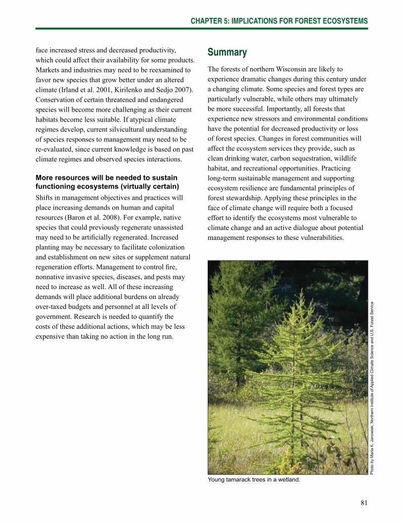
81
CHAPTER 5: IMPLICATIONS FOR FOREST ECOSYSTEMS
face increased stress and decreased productivity, which could affect their availability for some products. Markets and industries may need to be reexamined to favor new species that grow better under an altered climate (Irland et al. 2001, Kirilenko and Sedjo 2007). Conservation of certain threatened and endangered species will become more challenging as their current habitats become less suitable. If atypical climate regimes develop, current silvicultural understanding of species responses to management may need to be re-evaluated, since current knowledge is based on past climate regimes and observed species interactions.
More resources will be needed to sustain functioning ecosystems (virtually certain)Shifts in management objectives and practices will place increasing demands on human and capital resources (Baron et al. 2008). For example, native species that could previously regenerate unassisted may need to be artifi cially regenerated. Increased planting may be necessary to facilitate colonization and establishment on new sites or supplement natural regeneration efforts. Management to control fi re, nonnative invasive species, diseases, and pests may need to increase as well. All of these increasing demands will place additional burdens on already over-taxed budgets and personnel at all levels of government. Research is needed to quantify the costs of these additional actions, which may be less expensive than taking no action in the long run.
Summary
The forests of northern Wisconsin are likely to experience dramatic changes during this century under a changing climate. Some species and forest types are particularly vulnerable, while others may ultimately be more successful. Importantly, all forests that experience new stressors and environmental conditions have the potential for decreased productivity or loss of forest species. Changes in forest communities will affect the ecosystem services they provide, such as clean drinking water, carbon sequestration, wildlife habitat, and recreational opportunities. Practicing long-term sustainable management and supporting ecosystem resilience are fundamental principles of forest stewardship. Applying these principles in the face of climate change will require both a focused effort to identify the ecosystems most vulnerable to climate change and an active dialogue about potential management responses to these vulnerabilities.
Young tamarack trees in a wetland.
Pho
to b
y M
aria
K. J
anow
iak,
Nor
ther
n In
stitu
te o
f App
lied
Clim
ate
Sci
ence
and
U.S
. For
est S
ervi
ce
82
GLOSSARY
Adaptation: Adjustment in natural or human systems in response to actual or expected climatic stimuli or their effects, which moderates harm or exploits benefi cial opportunities (IPCC 2007).
Aerosol: A suspension of fi ne solid particles or liquid droplets in a gas, such as smoke, oceanic haze, air pollution, and smog. Aerosols may infl uence climate by either scattering and absorbing radiation; or by acting as condensation nuclei for cloud formation or modifying the properties and lifetime of clouds (IPCC 2007, King et al. 2007).
Analysis area: The portion of Wisconsin that falls within Ecological Province 212 (Mixed Laurentian Forest) of the National Hierarchical Framework of Ecological Units (Bailey 1995, ECOMAP 1993). When data was not available for this analysis area, data were selected for the 33 counties most analogous to Province 212: Ashland, Barron, Bayfi eld, Brown, Burnett, Chippewa, Clark, Door, Douglas, Florence, Forest, Iron, Kewaunee, Langlade, Lincoln, Manitowoc, Marathon, Marinette, Menominee, Oconto, Oneida, Outagamie, Polk, Portage, Price, Rusk, Sawyer, Shawano, Taylor, Vilas, Washburn, Waupaca, and Wood.
Bagging Trees: This statistical technique begins with a ‘regression tree’ approach, but recognizes that part of the output error in using a single regression tree comes from the specifi c selection of an original dataset. The bagging trees method uses another statistical technique called ‘bootstrapping’ to create several similar datasets. Regression trees are then produced from these new datasets and results are averaged.
Barrens: Plant communities that occur on sandy soils and are dominated by grasses, low shrubs, small trees, and scattered large trees (Curtis 1959).
Basefl ow: The condition of only groundwater providing the entire fl ow of a stream (during most of the year, streamfl ow is composed of both groundwater discharge and land surface runoff).
Biomass: The mass of living organic matter (plant and animal) in an ecosystem; biomass also refers to organic matter (living and dead) available on a renewable basis for use as a fuel; biomass includes trees and plants (both terrestrial and aquatic), agricultural crops and wastes, wood and wood wastes, forest and mill residues, animal wastes, livestock operation residues, and some municipal and industrial wastes (King et al. 2007).
Biome: A regional ecosystem with a distinct assemblage of vegetation, animals, microbes, and physical environment often refl ecting a certain climate and soil.
Boreal forest: Found only between 50-55 and 65-70 degrees latitude of the Northern Hemisphere, the boreal forests are adapted to cool northern temperatures and low rainfall (below 500mm; FAO 2001).
Carbon dioxide fertilization: Increased plant uptake of carbon dioxide through photosynthesis in response to higher concentrations of atmospheric carbon dioxide (Norby et al. 2005).
Cavitation: Percent loss of hydraulic conductivity, or the process by which xylem vessels become air-fi lled, resulting in reduced water transport (Zhu et al. 2000).
Composite products: Roundwood logs, bolts, and chips used in the manufacture of reconstituted wood products (chip board, fl ake board, oriented strand board (OSB), engineered lumber, etc.). Principal species used in composite products include aspen, jack pine, and birch.
83
GLOSSARY
Conifer: Any gymnosperm tree or shrub of the phylum Coniferophyta, typically bearing cones and evergreen leaves. The group includes the pines, spruces, fi rs, larches, yews, junipers, cedars, cypresses, and sequoias.
Derecho: Widespread and long-lived windstorm that is associated with a band of rapidly moving showers or thunderstorms.
Downscaling: A method for obtaining high-resolution climate or climate change information from relatively coarse-resolution global climate models; involves examining the statistical relationship between past climate data and on-the-ground measurements.
Disturbance: Stresses and destructive agents such as invasive species, diseases, and fi re; changes in climate and serious weather events such as hurricanes and ice storms; pollution of the air, water, and soil; real estate development of forest lands; and timber harvest. Some of these are caused by humans, in part or entirely, others are not.
Driver: Any natural or human-induced factor that directly or indirectly causes a change in an ecosystem (Carpenter et al. 2006).
Eastern deciduous forest: Dominated by deciduous trees such as oaks, maples, beech, hickories, and birches that drop their leaves. Softwoods do live in this forest, but they are rarely dominant. This forest develops under cold winters (but not as cold as the boreal region to the north), and annual rainfall is higher in this forest than anywhere else in north America except for the subtropical and tropical areas to the south.
Ecological processes: Processes fundamental to the functioning of a healthy and sustainable ecosystem, usually involving the transfer of energy and substances from one medium or trophic level to another.
Ecoregion: Repetitive pattern of ecosystems associated with commonalities in soil and landform that characterize that larger region.
Edaphic: Of or pertaining to soil characteristics.
Emissions scenario: A plausible representation of the future development of emissions of greenhouse gases and aerosols that are potentially radiatively active, based on certain demographic, technological, or environmental developments (IPCC 2007, King et al. 2007).
Ensemble average: The average value of a large number of output values from a climate model; a way to address some of the uncertainties in the system.
Evapotranspiration: The sum of evaporation and plant transpiration from the Earth’s land surface to atmosphere.
Excelsior: A product made of wood slivers, cut from logs, mainly used in packaging, for the cooling pads in home evaporative cooling systems known as swamp coolers, for erosion control mats, or as a raw material for the production of other products such as bonded wood wool boards.
Extirpation: Local extinction or loss of a species from an area.
Fen: A peat-forming wetland fed by sources other than precipitation, such as drainage from surrounding mineral soils or groundwater movement.
Fire-return interval: The number of years between two successive fi re events at a specifi c location.
Forest type: A classifi cation of forest land based on the dominant species present, as well as associate species commonly occurring with the dominant species (Perry et al. 2004).
Forest type group: Based on FIA defi nitions, a combination of forest types that share closely associated species or site requirements and are generally combined for brevity of reporting (Perry et al. 2004).
Fragipan: A natural subsurface horizon with very low organic matter, high bulk density, is slowly or very slowly permeable to water, is considered root restricting, and usually has few to many bleached, roughly vertical planes which are faces of coarse or very coarse polyhedrons or prisms. A fragipan has hard or very hard consistence (seemingly cemented) when dry but shows a moderate to weak brittleness when moist (SAF 2008).
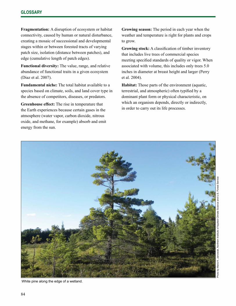
84
GLOSSARY
Fragmentation: A disruption of ecosystem or habitat connectivity, caused by human or natural disturbance, creating a mosaic of successional and developmental stages within or between forested tracts of varying patch size, isolation (distance between patches), and edge (cumulative length of patch edges).
Functional diversity: The value, range, and relative abundance of functional traits in a given ecosystem (Diaz et al. 2007).
Fundamental niche: The total habitat available to a species based on climate, soils, and land cover type in the absence of competitors, diseases, or predators.
Greenhouse effect: The rise in temperature that the Earth experiences because certain gases in the atmosphere (water vapor, carbon dioxide, nitrous oxide, and methane, for example) absorb and emit energy from the sun.
Growing season: The period in each year when the weather and temperature is right for plants and crops to grow.
Growing stock: A classifi cation of timber inventory that includes live trees of commercial species meeting specifi ed standards of quality or vigor. When associated with volume, this includes only trees 5.0 inches in diameter at breast height and larger (Perry et al. 2004).
Habitat: Those parts of the environment (aquatic, terrestrial, and atmospheric) often typifi ed by a dominant plant form or physical characteristic, on which an organism depends, directly or indirectly, in order to carry out its life processes.
White pine along the edge of a wetland.
Pho
to b
y M
aria
K. J
anow
iak,
Nor
ther
n In
stitu
te o
f App
lied
Clim
ate
Sci
ence
and
U.S
. For
est S
ervi
ce
85
GLOSSARY
Hardwood: A dicotyledonous tree, usually broad-leaved and deciduous. Hardwoods can be split into soft hardwoods—red maple, paper birch, quaking aspen and American elm; and hard hardwoods—sugar maple, yellow birch, black walnuts, and oaks (Perry et al. 2004).
Hydraulic gradient: The slope of the water, or the drop in pressure head per length in the direction of streamfl ow (SAF 2008).
Hydrophytic vegetation: Plant life that occurs in areas where the frequency and duration of inundation or soil saturation produce permanently or periodically saturated soils of suffi cient duration to exert a controlling infl uence on the plant species present.
Impact model: Simulations of impacts on trees, animals, and ecosystems; these models use GCM projections as inputs, and include additional inputs such as tree species, soil types, and life history traits of individual species.
Importance value: An index of the relative abundance of a species in a given community (0 = least abundant, 50 = most abundant).
Industry-owned forest: Land owned by forest product companies that harvest and market timber.
Intensity: Amount of precipitation falling per unit of time.
Kyoto Protocol: Adopted at the 1997 Third Session of the Conference of Parties to the UN Framework Convention on Climate Change in Kyoto, Japan; it contains legally binding commitments to reduce anthropogenic greenhouse gas emissions by at least 5 percent below 1990 levels in the period 2008-2012 (IPCC 2007).
Lacustrine clay deposits: Pertaining to or formed in a lake; usually softer than adjacent tills and often show clear horizontal parting of silt or fi ne sand.
Landtype Association: The characterization of landscapes from Sections and Subsections into further refi ned units that describe the composition of landscapes by similarities and repeatable patterns in landforms, their dominant formative processes, and underlying geologic materials.
Mesic: Characterized as requiring a moderate amount of water.
Mesophication: “Whereby microenvironmental conditions (cool, damp, and shaded conditions; less fl ammable fuel beds) continually improve for shade-tolerant mesophytic species and deteriorate for shade-intolerant, fi re-adapted species” (Nowacki and Abrams 2008).
Minerotrophic: Groundwater-fed; areas infl uenced by groundwater that has been in contact with soil or bedrock and is richer in mineral nutrients than rainwater.
Model error: Uncertainty caused by a lack of complete understanding of some climate processes, or by the inability of models to pick up small-scale but infl uential climate processes.
Model reliability score: For the Tree Atlas: a ‘tri-model’ approach to assess reliability of model predictions for each species, classifi ed as high, medium, or low depending on the assessment of the stability of the bagged trees and the R2 in RandomForest (Iverson et al. 2009).
Modifying factor: Environmental variables (i.e., site conditions, interspecies competition, disturbance, dispersal ability, etc.) that infl uence the way a tree may respond to climate change.
Nonindustrial private landowners: An ownership class of private lands where the owner does not operate wood-using plants (Perry et al. 2004).
Northern hardwoods: Forest group with wet-mesic to dry-mesic soils, medium to high soil nutrient level, and supporting trees species such as sugar maple (dominant), basswood, eastern hemlock, yellow birch, eastern hophornbeam, red maple, and white ash.
Parcelization: The subdivision of a single forest ownership into two or more ownerships. Parcelization may result in fragmentation if habitat is altered under new ownership.
Peak fl ow: The maximum instantaneous discharge of a stream or river at a given location.
86
GLOSSARY
Pioneer species: a plant capable of invading bare sites (e.g., newly exposed soil) and persisting there until supplanted by successional species, or any new arrival in the early stages of succession.
Plasticity: The ability of an organism to change its characteristics (gene expression or behavior) in response to changes in the environment.
Phenology: The study of the timing of natural events such as the date that migrating birds return, the fi rst fl ower dates for plants, and the date on which a lake freezes in the autumn or opens in the spring.
Projection: A model-derived estimate of future climate, and the pathway leading to it.
Process model: A model that relies on computer simulations based on mathematical representations of physical and biological processes that interact over space and time.
Proxy: Ice and sediment cores, tree rings, and pollen fossils are all examples of things that can be analyzed to infer past climate. The size of rings and the isotopic ratios of elements (e.g., oxygen, hydrogen, and carbon) in rings and other substrates allow scientists to infer climate and timing.
Pulpwood: Roundwood, whole-tree chips, or wood residues used for the production of wood pulp for making paper and paperboard products (Perry et al. 2004). Principal pulpwood species are aspen, maples, jack pine, red pine, birch, and fi r.
RandomForests: The RandomForest is a statistical technique similar to Bagging Trees in that it also uses bootstrapping to construct multiple regression trees. The difference is that each tree is produced with a random subset of predictors. Typically, 500 to 2,000 trees are produced and the results are aggregated by averaging. This technique eliminates the possibility of overfi tting data.
Real Estate Investment Trust (REIT): Considered a nonindustrial landowner.
Realized niche: The portion of potential habitat a species occupies; usually it less than what is available because of predation, disease, and competition with other species.
Recharge: The natural process of movement of rainwater from land areas or streams through permeable soils into water-holding rocks that provide underground storage (i.e., aquifers).
Refugia: Locations and habitats that support populations of organisms that are limited to small fragments of their previous geographic range.
Resilience: The ability of a social or ecological system to absorb disturbances while retaining the same basic structure and ways of functioning, the capacity for self-organization, and the capacity to adapt to stress and change (IPCC 2007).
Roundwood: Logs, bolts, and other round timber generated from harvesting trees for industrial or consumer use (Perry et al. 2004).
Runoff: That part of the precipitation that appears in surface streams. It is the same as streamfl ow unaffected by artifi cial diversions or storage.
Saw log: A log meeting minimum standards of diameter, length, and defect, including logs at least 8 feet long, sound and straight, and with a minimum diameter inside bark of 6 inches for softwoods and 8 inches for hardwoods, or meeting other combinations of size and defect specifi ed by regional standards (Perry et al. 2004).
Sawtimber: A live tree of commercial species containing at least a 12-foot saw log or two noncontiguous 8-foot or longer saw logs, and meeting specifi cations for form; softwoods must be at least 9 inches, and hardwoods must be at least 11 inches, respectively, in diameter outside the bark (Perry et al. 2004).
87
GLOSSARY
Scenario: A coherent, internally consistent and plausible description of a possible future state of the world. It is not a forecast; rather, each scenario is one alternative image of how the future can unfold. A projection may serve as the raw material for a scenario, but scenarios often require additional information (IPCC 2007).
Severity: The proportion of aboveground vegetation killed and the degree of forest fl oor and soil disruption (Oliver and Larson 1996).
Softwood: A coniferous tree, usually evergreen, having needles or scale-like leaves (Perry et al. 2004).
Snowpack: Layers of accumulated snow that usually melt during warmer months.
Species distribution model: A model that uses statistical relationships to project future change.
Stochastic: Patterns resulting from random effects.
Stratosphere: The layer of the Earth’s atmosphere which lies between 10 and 50 kilometers above the Earth.
Streamfl ow: Discharge that occurs in a natural surface stream course whether or not it is diverted or regulated.
Stormfl ow: Runoff that occurs due to a heavy precipitation event.
Succession: The gradual supplanting of one community of plants by another. Early successional or “pioneer” species typically produce a great quantity of seeds and that are capable to germinate and grow under direct sunlight. Once they have produced a closed canopy, the lack of direct sunlight makes it diffi cult for seedlings to develop. It is then the opportunity for shade “tolerant” species to get established. When these pioneers die, the shade tolerants will replace them. The shade tolerant species are capable of growing under the canopy, and therefore, in the absence of catastrophes, will stay to become the late successional species.
Super-canopy: A level of canopy formed above the main upper canopy, such as the highest canopy of eastern white pine.
Tension zone: A transitional band that corresponds to a number of climatic factors. Vegetation north and south of the tension zone refl ect habitat conditions as a result of climatic differences.
Threat: A source of danger or harm.
Till: Unstratifi ed soil deposited by a glacier; consists of sand and clay and gravel and boulders mixed together.
Timber Investment Management Organization (TIMO): Considered a nonindustrial landowner.
Troposphere: The lowest part of the atmosphere from the surface to about 10 kilometers in altitude in mid-latitudes (ranging from 9 kilometers in high latitudes to 16 kilometers in the tropics on average) where clouds and “weather” phenomena occur.
Topkill: Death of above-ground tree stem and branches.
Uncertainty: A term used to describe the range of possible values around a best estimate, sometimes expressed in terms of probability or likelihood (King et al. 2007).
Veneer: A roundwood product from which veneer is sliced or sawn and that usually meets certain standards of minimum diameter, length, and maximum defect. Principal veneer species are maple, aspen, birch, oaks, and black walnut.
Vulnerability: The degree to which a system is susceptible to, and unable to cope with, adverse effects of climate change, including climate variability and extremes. Vulnerability is a function of the character, magnitude, and rate of climate change and variation to which a system is exposed, its sensitivity, and its adaptive capacity (IPCC 2007).
88
LITERATURE CITED
Aber, J.R.; Neilson, P.; McNulty, S.; Lenihan, J.M.; Bachelet, D.; Drapek, R.J. 2001. Forest processes and global environmental change: predicting the effects of individual and multiple stressors. BioScience. 51(9): 735-751.
Abrams, M.D. 1998. The red maple paradox. BioScience. 48(5): 355.
Ainsworth, E.A.; Long, S.P. 2005. What have we learned from 15 years of free-air CO2 enrichment (FACE)? A meta-analytic review of the responses of photosynthesis, canopy properties and plant production to rising CO2. New Phytologist. 165(2): 351-372.
Ainsworth, E.A.; Rogers, A. 2007. The response of photosynthesis and stomatal conductance to rising [CO2]: mechanisms and environmental interactions. Plant, Cell & Environment. 30(3): 258-270.
Albert, D.A.; Denton, S.R.; Barnes, B.V.; Simpson, K.E. 1986. Regional landscape ecosystems of Michigan. Ann Arbor, MI: University of Michigan, School of Natural Resources. 32 p.
Alverson, W.S.; Waller, D.M.; Solheim, S.L. 1988. Forests too deer: edge effects in northern Wisconsin. Conservation Biology. 2(4): 348-358.
Anderson, H.W.; Hoover, M.D.; Reinhart, K.G. 1976. Forests and water: effects of forest management on fl oods, sedimentation, and water supply. Gen. Tech. Rep. PSW-018. Berkeley, CA: U.S. Department of Agriculture, Forest Service, Pacifi c Southwest Forest and Range Experiment Station. 115 p.
Ayers, M.P.; Lombardero, M.J. 2000. Assessing the consequences of global change for forest disturbance from herbivores and pathogens. Science of the Total Environment. 262(3): 263-286.
Backlund, P.; Janetos, A.; Schhimel, D. 2008. The Effects of Climate Change on Agriculture, Land Resources, Water Resources and Biodiversity in the United States. In: Walsh, M., ed. Synthesis and Assessment Product 4.3 Washington, DC: U.S. Climate Change Science Program and the Subcommittee on Global Change Research. 240 p.
Bailey, R.G. 1995. Description of the ecoregions of the United States. Misc. Publ. 1391. Washington, DC: U.S. Department of Agriculture, Forest Service. 108 p.
Bawa, K.S.; Dayanandan, S. 1998. Global climate change and tropical forest genetic resources. Climatic Change. 39(2): 473-485.
Becker, G.C. 1983. Fishes of Wisconsin. Madison, WI: University of Wisconsin Press. 1052 p.
Berz, G.A. 1993. Global warming and the insurance industry. Interdisciplinary Science Reviews. 18: 120-125.
Bhiry, N.; Filion, L. 1996. Mid-holocene hemlock decline in eastern North America linked with phytophagous insect activity. Quaternary Research. 45(3): 312-320.
Boelter, D.H.; Verry, E.S. 1977. Peatland and water in the northern Lake States. Gen. Tech. Rep. NC-31. St. Paul, MN: U.S. Department of Agriculture, Forest Service, North Central Forest Experiment Station. 22 p.
89
LITERATURE CITED
Bohlen, P.J.; Scheu, S.; Hale, C.M.; McLean, M.A.; Migge, S.; Groffman, P.M.; Parkinson, D. 2004. Non-native invasive earthworms as agents of change in northern temperate forests. Frontiers in Ecology and the Environment. 2(8): 427-435.
Bonan, G.B. 2008. Forests and climate change: forcings, feedbacks, and the climate benefi ts of forests. Science. 320(5882): 1444-1449.
Bradley, N.L.; Leopold, A.C.; Ross, J.; Huffaker, W. 1999. Phenological changes refl ect climate change in Wisconsin. Proceedings of the National Academy of Sciences of the United States of America. 96(17): 9701-9704.
Burnett, A.W.; Kirby, M.E.; Mullins, H.T.; Patterson, W.P. 2003. Increasing Great Lake-effect snowfall during the twentieth century: a regional response to global warming? Journal of Climate. 16(21): 3535-3542.
Camill, P.; Clark, J.S. 2000. Long-term perspectives on lagged ecosystem responses to climate change: permafrost in boreal peatlands and the grassland/woodland boundary. Ecosystems. 3(6): 534-544.
Campbell, J.L.; Rustad, L.E.; Boyer, E.W.; Christopher, S.F.; Driscoll, C.T.; Fernandez, I.J.; Groffman, P.M.; Houle, D.; Kiekcusch, J.; Magill, A.H.; Mitchell, M.J.; Ollinger, S.V. 2009. Consequences of climate change for biogeochemical cycling in forests of northeastern North America. Canadian Journal of Forest Research. 39: 264-284.
Canham, C.D.; Loucks, O.L. 1984. Catastrophic windthrow in the presettlement forests of Wisconsin. Ecology. 65(3): 803-809.
Carpenter, S.R.; Bennett, E.M.; Peterson, G.D. 2006. Editorial: special feature on scenarios for ecosystem services. Ecology and Society. 11(2): 32. Available at http://www.ecologyandsociety.org/vol11/iss2/art32/. (Accessed Feb. 2, 2011).
Clark, J.S.; Fastie, C.; Hurtt, G.; Jackson, S.T.; Johnson, C.; King, G.A.; Lewis, M.; Jason, L.; Pacala, S.; Prentice, C.; Schupp, E.W.; Webb, T., III; Wyckoff, P. 1998. Reid’s paradox of rapid plant migration. BioScience. 48(1): 13-24.
Cleland, D.T.; Leefers, L.A.; Dickmann, D.I. 2001. Ecology and management of aspen: a Lake States perspective. In: Shepperd, W.D., ed. Sustaining aspen in western landscapes: Symposium proceedings. [Fort Collins, CO]: U.S. Department of Agriculture, Forest Service, Rocky Mountain Research Station: 81-100.
Cleland, D.T.; Brosofske, K.D.; Mclean, A.M. 2008. Comparison of historical and modern fi re rotations of the Lake States. Unpublished manuscript.
Climate Change Science Program [CCSP]. 2008. Preliminary review of adaptation options for climate-sensitive ecosystems and resources. A report by the U.S. Climate Change Science Program and the subcommittee on Global Change Research. [Julius, S.H., J.M. West (eds.), J.S. Baron, B. Griffi th, L.A. Joyce, P. Kareiva, B.D. Keller, M.A. Palmer, C.H. Peterson, and J.M. Scott (Authors)]. Washington, DC: U.S. Environmental Protection Agency. 873 p.
Cole, C.T.; Anderson, J.; Lindroth, R.L.; Waller, D.M. 2010. Rising concentrations of atmospheric CO2 have increased growth in natural stands of quaking aspen (Populus tremuloides). Global Change Biology. 16(8): 2186-2197.
Coniglio, M.C.; Stensrud, D.J. 2004. Interpreting the climatology of derechos. Weather and Forecasting. 19(3): 595-605.
Cote, S.D.; Rooney, T.P.; Tremblay, J.P.; Dussault, C.; Waller, D.M. 2004. Ecological impacts of deer overabundance. Annual Review of Ecology Evolution and Systematics. 35: 113-147.
Cotton, P.A. 2003. Avian migration phenology and global climate change. Proceedings of the National Academy of Sciences. 100(21): 12219-12222.
90
LITERATURE CITED
Crow, T.R.; Buckley, D.S.; Nauertz, E.A.; Zasada, J.C. 2002. Effects of management on the composition and structure of northern hardwood forests in upper Michigan. Forest Science. 48(1): 129-145.
Curtis, J. 1959. The vegetation of Wisconsin. Madison, WI: University of Wisconsin Press. 640 p.
Dai, A.; Trenberth, K.E.; Qian, T. 2004. A global dataset of Palmer Drought Severity Index for 1870-2002: relationship with soil moisture and effects of surface warming. Journal of Hydrometeorology. 5: 1117-1129.
Dale, V.H.; Joyce, L.A.; McNulty, S.; Neilson, R.P.; Ayres, M.P.; Flannigan, M.D.; Hanson, P.J.; Irland, L.C.; Lugo, A.E.; Peterson, C.J.; Simberloff, D.; Swanson, F.J.; Stocks, B.J.; Wotton, B.M. 2001. Climate change and forest disturbances. BioScience. 51(9): 723-734.
Davis, M.B. 1981. Quaternary history and the stability of forest communities. In: West, D.C.; Shugart, H.H., eds. Forest succession: concepts and application. New York: Springer-Verlag: 132-153.
Davis, M.B. 1989. Lags in vegetation response to greenhouse warming. Climatic Change. 15(1): 75-82.
Davis, M.B.; Shaw, R.G. 2001. Range shifts and adaptive responses to quaternary climate change. Science. 292(5517): 673-679.
Davis, M.B.; Shaw, R.G.; Etterson, J.R. 2005. Evolutionary responses to changing climate. Ecology. 86(7): 1704-1714.
Davis, M.B.; Sugita, S.; Calcote, R.R.; Ferrari, J.B.; Frelich, L.E. 1993. Historical development of alternate communities in a hemlock-hardwood forest in northern Michigan, U.S.A. In: Edwards, P.J., ed. Large-scale ecology and conservation biology: the 35th symposium of the British Ecological Society with the Society for Conservation Biology. Oxford, UK: Blackwell Scientifi c Publications: 19-39.
Decker, K.L.M.; Wang, D.; Waite, C.; Scherbatskoy, T. 2003. Snow removal and ambient air temperature effects on forest soil temperatures in northern Vermont. Soil Science Society of America Journal. 67(4): 1234-1242.
Delcourt, P.A.; Delcourt, H.R. 1987. Late-quaternary dynamics of temperate forests: applications of paleoecology to issues of global environmental change. Quaternary Science Reviews. 6: 129-146.
Deller, S.C.; Williams, D. 2009. The contribution of agriculture to the Wisconsin economy. Madison, WI: University of Wisconsin Cooperative Extension. Available at http://www.uwex.edu/ces/ag/wisag/documents/Ag_Impacts_2007_FINAL_7%2031%2009.pdf. (Accessed Feb. 22, 2011).
Delworth, T.L.; Broccoli, A.J.; Rosati, A.; Stouffer, R.J.; Balaji, V.; Beesley, J.A.; Cooke, W.F.; Dixon, K.W.; Dunne, J.; Dunne, K.A.; Durachta, J.W.; Findell, K.L.; Ginoux, P.; Gnanadesikan, A.; Gordon, C.T.; Griffi es, S.M.; Gudgel, R.; Harrison, M.J.; Held, I.M.; Hemler, R.S.; Horowitz, L.W.; Klein, S.A.; Knutson, T.R.; Kushner, P.J.; Langenhorst, A.R.; Lee, H.C.; Lin, S.J.; Lu, J.; Malyshev, S.L.; Milly, P.C.D.; Ramaswamy, V.; Russell, J.; Schwarzkopf, M.D.; Shevliakova, E.; Sirutis, J.J.; Spelman, M.J.; Stern, W.F.; Winton, M.; Wittenberg, A.T.; Wyman, B.; Zeng, F.; Zhang, R. 2006. GFDL’s CM2 global coupled climate models. Part I: Formulation and simulation characteristics. Journal of Climate. 19(5): 643-674.
Department of Agriculture Trade and Consumer Protection [DATCP]. 2010. Wisconsin’s emerald ash borer information source. Madison, WI: Department of Agriculture Trade and Consumer Protection. Available at http://www.emeraldashborer.wi.gov/article.jsp?topicid=13. (Accessed Feb. 22, 2011).

91
LITERATURE CITED
Diaz, S.; Lavorel, S.; Bello, F.D.; Quetier, F.; Grigulis, K.; Robson, T.M. 2007. Incorporating plant functional diversity effects in ecosystem service assessments. Proceedings of the National Academy of Sciences. 104(52): 20684-20689.
Donner, D.M.; Ribic, C.A.; Probst, J.R. 2009. Male Kirtland’s warblers’ patch-level response to landscape structure during periods of varying population size and habitat amounts. Forest Ecology and Management. 258(7): 1093-1101.
Drake, B.G.; Gonzalez-Meler, M.A.; Long, S.P. 1997. More effi cient plants: a consequence of rising atmospheric CO2? Annual Review of Plant Physiology and Plant Molecular Biology. 48(1): 609-639.
Dukes, J.S.; Pontius, J.; Orwig, D.; Garnas, J.R.; Rodgers, V.L.; Brazee, N.; Cooke, B.; Theoharides, K.A.; Stange, E.E.; Harrington, R.; Ehrenfeld, J.; Gurevitch, J.; Lerdau, M.; Stinson, K.; Wick, R.; Ayres, M. 2009. Responses of insect pests, pathogens, and invasive plant species to climate change in the forests of northeastern North America: What can we predict? Canadian Journal of Forest Research. 39(2): 231-248.
Easterling, D.R.; Wehner, M.F. 2009. Is the climate warming or cooling? Geophysical Research Letters. 36(L08706): 3. Available at http://www.agu.org/pubs/crossref/2009/2009GL037810.shtml. (Accessed Feb. 22, 2011).
Eckstein, R.; Dahl, G.; Easterly, S.; Ishmael, B.; Nelson, J.; Manthey, P.; Meyer, M.; Tesky, L.; Goltz, D.; Glenzinski, B. 2008. Wisconsin bald eagle and osprey surveys. Madison, WI: Wisconsin Department of Natural Resources. 8. Available at http://dnr.wi.gov/org/land/wildlife/harvest/reports/eagleospreysurv08.pdf. (Accessed Feb. 22, 2011).
ECOMAP. 1993. National hierarchical framework of ecological units. Washington, DC: U.S. Department of Agriculture, Forest Service. 20 p.
Etterson, M.; Danz, N.; Lind, J.; Haowski, J.M.; Niemi, G.J. 2007. Breeding bird monitoring in Great Lakes national forest: 1991-2006. 2006 annual report to the Chequamegon/Nicolet, Chippewa, and Superior National Forests. Tech. Rep. NRRI/TR-2007/05. Duluth, MN: University of Minnesota, Natural Resources Research Institute. Available at http://www.nrri.umn.edu/mnbirds/reports/2006_AnnualReport.pdf. (Accessed Feb. 22, 2011).
Flannigan, M.; Stocks, B.; Turetsky, M.; Wotton, M. 2009. Impacts of climate change on fi re activity and fi re management in the circumboreal forest. Global Change Biology. 15(3): 549-560.
Flato, G.M.; Boer, G.J.; Lee, W.G.; McFarlane, N.A.; Ramsden, D.; Reader, M.C.; Weaver, A.J. 2000. The Canadian Centre for Climate Modelling and Analysis global coupled model and its climate. Climate Dynamics. 16(6): 451-467.
Forester, J.D.; Anderson, D.P.; Turner, M.G. 2008. Landscape and local factors affecting northern white cedar (Thuja occidentalis) recruitment in the Chequamegon-Nicolet National Forest, Wisconsin (U.S.A.). The American Midland Naturalist. 160(2): 438-453.
Foster, J.R.; Burton, J.I.; Forrester, J.A.; Liu, F.; Muss, J.D.; Sabatini, F.M.; Scheller, R.M.; Mladenoff, D.J. 2010. Evidence for a recent increase in forest growth is questionable. Proceedings of the National Academy of Sciences. 107(21): E86-87.
Frelich, L.E.; Reich, P.B. 2010. Will environmental changes reinforce the impact of global warming on the prairie-forest border of central North America? Frontiers in Ecology and the Environment. 8(7): 371-378.
Frelich, L.E.; Reich, P.B. 1996. Old growth in the Great Lakes region. In: Davis, M.B., ed. Eastern old growth forests. Washington, DC: Island Press: 144-160.
92
LITERATURE CITED
Gedney, N.; Cox, P.M.; Betts, R.A.; Boucher, O.; Huntingford, C.; Stott, P.A. 2006. Detection of a direct carbon dioxide effect in continental river runoff records. Nature. 439(7078): 835-838.
Gonzalez-Abraham, C.; Radeloff, V.; Hammer, R.; Hawbaker, T.; Stewart, S.; Clayton, M. 2007. Building patterns and landscape fragmentation in northern Wisconsin, USA. Landscape Ecology. 22(2): 217-230.
Graham, R.L.; Turner, M.G.; Dale, V.H. 1990. How increasing CO2 and climate change affect forests. BioScience. 40(8): 575-587.
Green, J.C. 1995. Birds and forests: a management and conservation guide. St. Paul, MN: Minnesota Department of Natural Resources. 182 p.
Gundale, M.J. 2002. Infl uence of exotic earthworms on the soil organic horizon and the rare fern Botrychium mormo. Conservation Biology. 16(6): 1555-1561.
Hale, C.; Frelich, L.; Reich, P.; Pastor, J. 2008. Exotic earthworm effects on hardwood forest fl oor, nutrient availability and native plants: a mesocosm study. Oecologia. 155(3): 509-518.
Hansen, J.; Ruedy, R.; Sato, M.; Lo, K. 2010. If it’s that warm, how come it’s so darned cold? Available at http://www.columbia.edu/~jeh1/mailings/2010/20100115_Temperature2009.pdf. (Accessed Feb. 22, 2011).
Hanson, P.J.; Weltzin, J.F. 2000. Drought disturbance from climate change: response of United States forests. The Science of the Total Environment. 262(3): 205-220.
Hardy, J.; Groffman, P.; Fitzhugh, R.; Henry, K.; Welman, A.; Demers, J.; Fahey, T.; Driscoll, C.; Tierney, G.; Nolan, S. 2001. Snow depth manipulation and its infl uence on soil frost and water dynamics in a northern hardwood forest. Biogeochemistry. 56(2): 151-174.
Hayhoe, K.; Wake, C.P.; Huntington, T.G.; Luo, L.F.; Schwartz, M.D.; Sheffi eld, J.; Wood, E.; Anderson, B.; Bradbury, J.; DeGaetano, A.; Troy, T.J.; Wolfe, D. 2007. Past and future changes in climate and hydrological indicators in the US Northeast. Climate Dynamics. 28(4): 381-407.
Heitzman, E.; Pregitzer, K.S.; Miller, R.O.; Lanasa, M.; Zuidema, M. 1999. Establishment and development of northern white-cedar following strip clearcutting. Forest Ecology and Management. 123(2-3): 97-104.
Heller, N.E.; Zavaleta, E.S. 2009. Biodiversity management in the face of climate change: a review of 22 years of recommendations. Biological Conservation. 142(1): 14-32.
Hellmann, J.J.; Byers, J.E.; Bierwagen, B.G.; Dukes, J.S. 2008. Five potential consequences of climate change for invasive species. Conservation Biology. 22(3): 534-543.
Hole, F.D. 1968. Soils of Wisconsin. Madison, WI: University of Wisconsin Press. 223 p.
Host, G.E.; Polzer, P.L.; Cleland, D.T. 1995. Regional climatic analysis of the northern Lake States. Tech. Rep. NRRI/TR-95/32. Duluth, MN: University of Minnesota, Natural Resources Research Institute. Available at http://www.ncrs.fs.fed.us/gla/reports/climate.htm. (Accessed Feb. 22, 2011).
Howe, R.W.; Roberts, L.J. 2005. Sixteen years of habitat-based bird monitoring in the Nicolet National Forest. In: Ralph, C.J.; Rich, T.D., eds. Bird conservation implementation and integration in the Americas: Proceedings of the third international partners in fl ight conference. Gen. Tech. Rep. PSW-GTR-191. Albany, CA: U.S. Department of Agriculture, Forest Service, Pacifi c Southwest Research Station: 963-973.
Huntington, T.G. 2008. CO2-induced suppression of transpiration cannot explain increasing runoff. Hydrological Processes. 22: 311-314.
93
LITERATURE CITED
Huntington, T.G.; Hodgkins, G.A.; Keim, B.D.; Dudley, R.W. 2004. Changes in the proportion of precipitation occurring as snow in New England (1949-2000). Journal of Climate. 17(13): 2626-2636.
Huntington, T.G.; Richardson, A.D.; McGuire, K.J.; Hayhoe, K. 2009. Climate and hydrological changes in the northeastern United States: recent trends and implications for forested and aquatic ecosystems. Canadian Journal of Forest Research. 39: 199-212.
Ibanez, I.; Clark, J.S.; Dietz, M.C. 2008. Evaluating the sources of potential migrant species: implications under climate change. Ecological Applications. 18(7): 1664-1678.
Ibanez, I.; Clark, J.S.; Shannon, L.; Lambers, J.H.R. 2007. Exploiting temporal variability to understand tree recruitment response to climate change. Ecological Monographs. 77(2): 163-177.
Ice, G.G.; Stednick, J.D. 2004. A century of forest and wildland watershed lessons. Bethesda, MD: Society of American Foresters. 287 p.
Intergovernmental Panel on Climate Change [IPCC]. 2005. Guidance notes for lead authors of the IPCC fourth assessment report on addressing uncertainties. Geneva, Switzerland: Intergovernmental Panel on Climate Change. Available at http://www.ipcc.ch/pdf/supporting-material/uncertainty-guidance-note.pdf. (Accessed Feb. 28, 2011).
Intergovermental Panel on Climate Change [IPCC]. 2000. Special report on emission scenarios. In: Nakicenovic, N.; Swart, R., eds. United Kingdom: Cambridge University Press. Available at http://www.grida.no/publications/other/ipcc_sr/?src=/climate/ipcc/emission/. (Accessed Feb. 22, 2011).
Intergovermental Panel on Climate Change [IPCC]. 2007. Climate change 2007: Synthesis report. Contribution of working groups I, II, and III to the fourth assessment report of the Intergovernmental Panel on Climate Change [Core Writing Team, Pachauri, R.K. and Reisinger, A. (eds.)]. Geneva, Switzerland: Intergovermental Panel on Climate Change. 104 p. Available at http://www.ipcc.ch/publications_and_data/publications_ipcc_fourth_assessment_report_synthesis_report.htm. (Accessed Feb. 22, 2011).
Irland, L.C.; Adams, D.; Alig, R.; Betz, C.J.; Chen, C.-C.; Hutchins, M.; McCarl, B.A.; Skog, K.; Sohngen, B.L. 2001. Assessing socioeconomic impacts of climate change on U.S. forests, wood-product markets, and forest recreation. BioScience. 51(9): 753-764.
Isaacs, J.B.; Smeeding, T.M. 2009. The fi rst Wisconsin poverty report. Madison, WI: Institue for Research on Policy. 28 p. Available at http://www.irp.wisc.edu/research/WisconsinPoverty/pdfs/First_Wisconsin_Poverty_Report_Final-2.pdf. (Accessed Feb. 22, 2011).
Iverson, L.R.; Prasad, A.M. 2002. Potential redistribution of tree species habitat under fi ve climate change scenarios in the eastern US. Forest Ecology and Management. 155: 205-222.
Iverson, L.R.; Prasad, A.M.; Matthews, S. 2008a. Modeling potential climate change impacts on the trees of the northeastern United States. Mitigation and Adaptation Strategies for Global Change. 13(5): 487-516.
Iverson, L.R.; Prasad, A.M.; Matthews, S.N.; Peters, M. 2008b. Estimating potential habitat for 134 eastern US tree species under six climate scenarios. Forest Ecology and Management. 254(3): 390-406.
Iverson, L.R.; Schwartz, M.W.; Prasad, A.M. 2004a. How fast and far might tree species migrate in the eastern United States due to climate change? Global Ecology and Biogeography. 13(3): 209-219.
94
LITERATURE CITED
Iverson, L.R.; Schwartz, M.W.; Prasad, A.M. 2004b. Potential colonization of new available tree species habitat under climate change: an analysis for fi ve eastern US species. Landscape Ecology. 19: 787-799.
Johns, T.C.; Carnell, R.E.; Crossley, J.F.; Gregory, J.M.; Mitchell, J.F.B.; Senior, C.A.; Tett, S.F.B. [et al.]. 1997. The second Hadley Centre coupled ocean-atmosphere GCM: model description, spinup and validation. Climate Dynamics. 13(2): 103-134.
Joyce, L.; Blate, G.; McNulty, S.; Millar, C.; Moser, S.; Neilson, R.; Peterson, D. 2009. Managing for multiple resources under climate change: national forests. Environmental Management. 44(6): 1022-1032.
Karl, T.R.; Melillo, J.M.; Peterson, T.C., eds. 2009. Global climate change impacts in the United States: a state of knowledge report from the U.S. Global Change Research Program. New York: Cambridge University Press. 189 p.
Karnosky, D.F.; Zak, D.R.; Pregitzer, K.S.; Awmack, C.S.; Bockheim, J.G.; Dickson, R.E.; Hendrey, G.R.; Host, G.E.; King, J.S.; Kopper, B.J.; Kruger, E.L.; Kubiske, M.E.; Lindroth, R.L.; Mattson, W.J.; Mcdonald, E.P.; Noormets, A.; Oksanen, E.; Parsons, W.F.J.; Percy, K.E.; Podila, G.K.; Riemenschneider, D.E.; Sharma, P.; Thakur, R.; Sôber, A.; Sôber, J.; Jones, W.S.; Anttonen, S.; Vapaavuori, E.; Mankovska, B.; Heilman, W.; Isebrands, J.G. 2003a. Tropospheric O3 moderates responses of temperate hardwood forests to elevated CO2: a synthesis of molecular to ecosystem results from the Aspen FACE project. Functional Ecology. 17(3): 289-304.
Karnosky, D.F.; Percy, K.E.; Mankovska, B.; Prichard, T.; Noormets, A.; Dickson, R.E.; Jepsen, E.; Isebrands, J.G.; Karnosky, D.F.; Percy, K.E.; Chappelka, A.H.; Simpson, C.; Pikkarainen, J. 2003b. Ozone affects the fi tness of trembling aspen. Developments in Environmental Sciences. 3: 199-209.
Karnosky, D.F.; Pregitzer, K.S.; Zak, D.R.; Kubiske, M.E.; Hendrey, G.R.; Weinstein, D.; Nosal, M.; Percy, K.E. 2005. Scaling ozone responses of forest trees to the ecosystem level in a changing climate. Plant, Cell & Environment. 28(8): 965-981.
King, A.W.; Dilling, L.; Zimmerman, G.P.; Fairman, D.M.; Houghton, R.A.; Marland, G.; Rose, A.Z.; Wilbanks, T.J. 2007. The fi rst state of the carbon cycle report (SOCCR): The North American carbon budget and implications for the global carbon cycle. U.S. Climate Change Science Program synthesis and assessment product 2.2. Asheville, NC: National Oceanic and Atmospheric Administration, National Climatic Data Center. 242 p. Available at http://www.climatescience.gov/Library/sap/sap2-2/fi nal-report/default.htm. (Accessed May 30, 2011).
Kirilenko, A.P.; Sedjo, R.A. 2007. Climate change impacts on forestry. Proceedings of the National Academy of Sciences of the United States of America. 104(50): 19697-19702.
Kling, G.W.; Hayhoe, K.; Johnson, L.B.; Magnuson, J.J.; Polasky, S.; Robinson, S.K.; Shuter, B.J.; Wander, M.M.; Wuebbles, D.J.; Zak, D.R.; Lindroth, R.L.; Moser, S.C.; Wilson, M.L. 2003. Confronting climate change in the Great Lakes region: impacts on our communities and ecosystems. Cambridge, MA: Union of Concerned Scientists and Washington, DC: Ecological Society of America. Available at http://ucsusa.org/assets/documents/global_warming/greatlakes_fi nal.pdf. (Accessed Feb. 22, 2011).
Knight, J.; Kenney, J.J.; Folland, C.; Harris, G.; Jones, G.S.; Palmer, M.; Parker, D.; Scaife, A.; Stott, P. 2009. Do global temperature trends over the last decade falsify climate predictions? In: Peterson, T.C.; Baringer, M.O., eds. State of the climate in 2008. Bulletin of the American Meteorologic Society: 90(8): S22-S23.
95
LITERATURE CITED
Knudsen, G.J. 1963. History of beaver in Wisconsin. Misc. Res. Rep. 7 (PUBL-SS-407 1963). [Location of publisher unknown]: Wisconsin Conservation Department. 15 p. Available at http://images.library.wisc.edu/EcoNatRes/EFacs/DNRResearch/DNRRep007/reference/econatres.dnrrep007.i0001.pdf. (Accessed Feb. 22, 2011).
Kohn, B.E.; Ashbrenner, J.E. 1993. Beaver population surveys and trends in Wisconsin. Unpublished study 25. Madison, WI: Wisconsin Department of Natural Resources. 23 p. On fi le with: Chequamegon-Nicolet National Forest, 500 Hanson Lake Road, Rhinelander, WI 54501.
Kohn, B.E.; Payne, N.F.; Ashbrenner, J.E.; Les, B. 1993. The fi sher in Wisconsin. Tech. Bull. 183. Madison, WI: Wisconsin Department of Natural Resources. 24 p. Available at http://digital.library.wisc.edu/1711.dl/EcoNatRes.DNRBull183. (Accessed Feb. 22, 2011).
Kucharik, C.; Serbin, S.; Vavrus, S.; Hopkins, E.; Motew, M. 2010. Patterns of climate change across Wisconsin from 1950 to 2006. Physical Geography. 31(1): 1-28.
Kunkel, K.E.; Easterling, D.R.; Hubbard, K.; Redmond, K. 2004. Temporal variations in frost-free season in the United States: 1895-2000. Geophysical Research Letters. 31(L03201): 4 p. Available at http://academic.engr.arizona.edu/HWR/Brooks/GC572-2004/readings/kunkel.pdf. (Accessed Feb. 22, 2011).
Kunkel, K.E.; Westcott, N.E.; Kristovich, D.A.R. 2002. Assessment of potential effects of climate change on heavy lake-effect snowstorms near Lake Erie. Journal of Great Lakes Research. 28(4): 521-536.
Le Quéré, C.; Raupach, M.R.; Canadell, J.G.; Marland, G. 2009. Trends in the sources and sinks of carbon dioxide. Nature Geoscience. 2: 831-836.
Lee, T.D.; Barrett, J.P.; Hartman, B. 2005. Elevation, substrate, and the potential for climate-induced tree migration in the White Mountains, New Hampshire, USA. Forest Ecology and Management. 212(1-3): 75-91.
Magnuson, J.J.; Robertson, D.M.; Benson, B.J.; Wynne, R.H.; Livingstone, D.M.; Arai, T.; Assel, R.A. [et al.]. 2000. Historical trends in lake and river ice cover in the Northern Hemisphere. Science. 289(5485): 1743-1746.
Martin, K.J.; Lutz, R.S.; Worland, M. 2009. Golden-winged warbler habitat use and abundance in northern Wisconsin. The Wilson Journal of Ornithology. 119(4): 523-532.
Matthews, S.N.; Connors, R.J.; Iverson, L.R.; Prasad, A.M. 2004. Atlas of climate change effects in 150 bird species of the eastern United States. Gen. Tech. Rep. NE-318. Newtown Square, PA: U.S. Department of Agriculture, Forest Service, Northeastern Research Station. 340 p.
McCaffery, K.R.; Ashbrenner, J.E.; Creed, W.A.; Kohn, B.E. 1997. The aspen-ruffed grouse connection. Journal of Forestry. 95(8): 16-20.
McLachlan, J.S.; Clark, J.S.; Manos, P.S. 2005. Molecular indicators of tree migration capacity under rapid climate change. Ecology. 86(8): 2088-2098.
McLaughlin, J.F.; Hellmann, J.J.; Boggs, C.L.; Ehrlich, P.R. 2002. Climate change hastens population extinctions. Proceedings of the National Academy of Sciences of the United States of America. 99(9): 6070-6074.
McMahon, S.M.; Parker, G.G.; Miller, D.R. 2010. Evidence for a recent increase in forest growth. Proceedings of the National Academy of Sciences. 107(8): 3611-3615.
Miles, P.D. December 2, 2010. Forest Inventory EVALIDator webapplication version 4.01 beta. St. Paul, MN: U.S. Department of Agriculture, Forest Service, Northern Research Station. Available at http://fi atools.fs.fed.us/Evalidator4/tmattribute.jsp. (Accessed Feb. 22, 2011).
Millar, C.I.; Stephenson, N.L.; Stephens, S.L. 2007. Climate change and forests of the future: managing in the face of uncertainty. Ecological Applications. 17(8): 2145-2151.
96
LITERATURE CITED
Min, S.K.; Zhang, X.; Zwiers, F.W.; Hegerl, G.C. 2011. Human contribution to more-intense precipitation extremes. Nature. 470(7334): 378-381.
Mladenoff, D.J.; Schulte, L.A.; Bolliger, J. 2008. Broad-scale changes in the northern forests: from past to present. In: Waller, D.M.; Rooney, T.P., eds. The vanishing present: Wisconsin’s changing lands, waters, and wildlife. Chicago, IL: University of Chicago Press: 61-73.
Mladenoff, D.J.; Stearns, F. 1993. Eastern hemlock regeneration and deer browsing in the northern Great Lakes region: a re-examination and model simulation. Conservation Biology. 7(4): 889-900.
Mohan, J.E.; Cox, R.M.; Iverson, L.R. 2009. Composition and carbon dynamics of forests in northeastern North America in a future, warmer world. Canadian Journal of Forest Research. 39: 213-230.
Munck, I.A.; Smith, D.R.; Sickley, T.; Stanosz, G.R. 2009. Site-related infl uences on cone-borne inoculum and asymptomatic persistence of Diplodia shoot blight fungi on or in mature red pines. Forest Ecology and Management. 257(3): 812-819.
NASA Goddard Institute for Space Studies. 2010. 2009: second warmest year on record; end of warmest decade. Washington, DC: National Aeronautics and Space Administration. Available at http://www.giss.nasa.gov/research/news/20100121/. (Accessed Feb. 22, 2011).
National Oceanic and Atmospheric Administration [NOAA]. 2006. Climate of the states: Wisconsin. Climatography of the United States, No. 60: Washington DC: U.S. Department of Commerce, National Climatic Data Center, Environmental Data Service. Available at http://cdo.ncdc.noaa.gov/cgi-bin/climatenormals/climatenormals.pl?directive=prod_select2&prodtype=CLIM60&subrnum=. (Accessed Feb. 23, 2011).
National Oceanic and Atmospheric Administration [NOAA]. 2008. Breakthrough article on the fi rst climate model. Washington DC: U.S. Department of Commerce, National Oceanic and Atmostpheric Administration. Available at http://celebrating200years.noaa.gov/breakthroughs/climate_model/welcome.html. (Accessed Feb. 23, 2011).
Natural Resource Council [NRC]. 2008. Hydrologic effects of a changing forest landscape. Washington, DC: National Academies Press. 180 p.
Norby, R.; DeLucia, E.; Gielen, B.; Calfapietra, C.; Giardina, C.; King, J.; Ledford, J.; McCarthy, H.; Moore, D.; Ceulemans, R. 2005. Forest response to elevated CO2 is conserved across a broad range of productivity. Proceedings of the National Academy of Sciences. 102(50): 18052-18056.
Noss, R.F. 2001. Beyond Kyoto: forest management in a time of rapid climate change. Conservation Biology. 15(3): 578-590.
Nowacki, G.J.; Abrams, M.D. 2008. The demise of fi re and “mesophication” of forests in the eastern United States. BioScience. 58(2): 123-138.
Nowacki, G.J.; Abrams, M.D.; Lorimer, C.G. 1990. Composition, structure, and historical development of northern red oak stands along an edaphic gradient in north-central Wisconsin. Forest Science. 36: 276-292.
Ollinger, S.; Goodale, C.; Hayhoe, K.; Jenkins, J. 2008. Potential effects of climate change and rising CO2 on ecosystem processes in northeastern U.S. forests. Mitigation and Adaptation Strategies for Global Change. 13(5): 467-485.
Ostrom, M.E. 1981. Bedrock geology of Wisconsin. Madison, WI: Wisconsin Geologic and Natural History Survey, University of Wisconsin. Available at http://www.uwex.edu/wgnhs/bdrk.htm. (Accessed Feb. 23, 2011).
97
LITERATURE CITED
Paradis, A.; Elkinton, J.; Hayhoe, K.; Buonaccorsi, J. 2008. Role of winter temperature and climate change on the survival and future range expansion of the hemlock woolly adelgid (Adelges tsugae) in eastern North America. Mitigation and Adaptation Strategies for Global Change. 13(5): 541-554.
Parmesan, C.; Yohe, G. 2003. A globally coherent fi ngerprint of climate change impacts across natural systems. Nature. 421: 37-42.
Perry, C.H.; Everson, V.A.; Brown, I.K.; Cummings-Carlson, J.; Dahir, S.E.; Jepsen, E.A.; Kovach, J. [et al.]. 2008. Wisconsin’s forests, 2004. Resour. Bull. NRS-23. Newtown Square, PA: U.S. Department of Agriculture, Forest Service, Northern Research Station. 104 p.
Peterson, C.J. 2000. Catastrophic wind damage to North American forests and the potential impact of climate change. The Science of the Total Environment. 262: 287-311.
Peterson, G.C.; Allen, R.; Holling, C.S. 1998. Ecological resilience, biodiversity, and scale. Ecosystems. 1(1): 6-18.
Peterson, G.W. 1997. Diplodia blight of pines. For. Insect and Disease Leafl . 161. Washington, DC: U.S. Department of Agriculture, Forest Service. Available at http://www.na.fs.fed.us/spfo/pubs/fi dls/diplodia/diplodiafi dl.htm. (Accessed Feb. 23, 2011).
Petit, R.J.; Hu, F.S.; Dick, C.W. 2008. Forests of the past: a window to future changes. Science. 320(5882): 1450-1452.
Plummer, D.A.; Caya, D.; Frigon, A.; Gigure, H.; Paquin, M.; Biner, D.; Harvey, S.; de Elia, R. 2006. Climate and climate change over North America as simulated by the Canadian RCM. Journal of Climate. 19(13): 3112-3132.
Poland, T.M.; McCullough, D.G. 2006. Emerald ash borer: invasion of the urban forest and the threat to North America’s ash resource. Journal of Forestry. 104(3): 118-124.
Pope, V.; Gallani, M.L.; Rowntree, P.R.; Stratton, R.A. 2000. The impact of new physical parameterizations in the Hadley Centre climate model: HadAM3. Climate Dynamics. 16: 123-146.
Powers, M.D.; Nagel, L.M. 2009. Pennsylvania sedge cover, forest management and deer density infl uence tree regeneration dynamics in a northern hardwood forest. Forestry. 82(3): 241-254.
Prasad, A.M.; Iverson, L.R.; Matthews, S.N.; Peters, M. 2007. A climate change atlas for 134 forest tree species of the eastern United States [Database]. Newtown Square, PA: U.S. Department of Agriculture, Forest Service, Northern Research Station. Available at http://www.nrs.fs.fed.us/atlas/tree/. (Accessed Feb. 23, 2011).
Pregitzer, K.S.; Burton, A.J.; King, J.S.; Zak, D.R. 2008. Soil respiration, root biomass, and root turnover following long-term exposure of northern forests to elevated atmospheric CO2 and tropospheric O3. New Phytologist. 180(1): 153-161.
Rabinowitz, D. 1981 Seven forms of rarity. In: Synge, H., ed. The biological aspects of rare plant conservation. New York: Wiley: 205-217.
Radeloff, V.C.; Mladenoff, D.J.; Hong, S.H.; Boyce, M.S. 1999. Forest landscape change in the northwestern Wisconsin Pine Barrens from pre-European settlement to the present. Canadian Journal of Forest Research. 29(11):1649-1659.
Radeloff, V.C.; Hammer, R.B.; Stewart, S.I. 2005. Rural and suburban sprawl in the US Midwest from 1940 to 2000 and its relation to forest fragmentation. Conservation Biology. 19(3): 793-805.
Reusch, T.B.H.; Ehlers, A.; Hammerli, A.; Worm, B. 2005. Ecosystem recovery after climatic extremes enhanced by genotypic diversity. Proceedings of the National Academy of Sciences. 102(8): 2826-2831.
98
LITERATURE CITED
Rhoads, A.G.; Hamburg, S.P.; Fahey, T.J.; Siccama, T.G.; Hane, E.N.; Battles, J.; Cogbill, C.; Randall, J.; Wilson, G. 2002. Effects of an intense ice storm on the structure of a northern hardwood forest. Canadian Journal of Forest Research. 32(10): 1763-1775.
Rich, R.L.; Frelich, L.E.; Reich, P.B. 2007. Wind-throw mortality in the southern boreal forest: effects of species, diameter and stand age. Journal of Ecology. 95: 1261-1273.
Richardson, A.D.; Bailey, A.S.; Denny, E.G.; Martin, C.W.; O’Keefe, J. 2006. Phenology of a northern hardwood forest canopy. Global Change Biology. 12(7): 1174-1188.
Richardson, K.; Steffen, W.; Schellnhuber, H.J.; Alcamo, J.; Barker, T.; Kammen, D.; Leemans, R.; Liverman, D.; Monasinghe, M.; Osman-Elasha, B.; Stern, N.; Waever, O. 2009. Climate change: global risks challenges and decisions. University of Copenhagen. http://edepot.wur.nl/10197. (Accessed Feb. 23, 2011).
Rickenbach, M.; Steele, T.W. 2006. Logging fi rms, nonindustrial private forests, and forest parcelization: evidence of fi rm specialization and its impact on sustainable timber supply. Canadian Journal of Forest Research. 36(1): 186-194.
Ritchie, J.C. 1986. Climate change and vegetation response. Plant Ecology. 67(2): 65-74.
Robbins, S.D. 1991. Wisconsin birdlife: population and distribution past and present. Madison, WI: University of Wisconsin Press. 702 p.
Robbins, S.D. 1997. Wisconsin’s neotropical migrant forest birds: breeding bird survey data 1966-1994. U.S. Fish and Wildlife Service. On fi le with: Chequamegon-Nicolet National Forest, 500 Hanson Lake Road, Rhinelander, WI 54501.
Robertson, D.M.; Ragotzkie, R.A.; Magnuson, J.J. 1992. Lake ice records used to detect historical and future climatic changes. Climatic Change. 21(4): 407-427.
Rodenhouse, N.L. 2009. Climate change effects on native fauna of northeastern forests. Canadian Journal of Forest Research. 39(2): 249-263.
Rogers, D.A.; Rooney, T.P.; Olson, D.; Waller, D.M. 2008. Shifts in southern Wisconsin forest canopy and understory richness, composition, and heterogeneity. Ecology. 89: 2482-2492.
Rolley, R.E. 2009. White-tailed deer population status 2008. Wisconsin Department of Natural Resources. Available at http://dnr.wi.gov/org/land/wildlife/harvest/reports/wtaildeerpop08.pdf. (Accessed Feb. 23, 2011).
Rolley, R.E.; Olson, J.F.; Worland, M.L. 2008. Beaver population analysis 2008. Wisconsin Department of Natural Resources. Available at http://dnr.wi.gov/org/land/wildlife/harvest/reports/08beaverpop.pdf. (Accessed Feb. 23, 2011).
Rooney, T.P.; McCormick, R.J.; Solheim, S.L.; Waller, D.M. 2000. Regional variation in recruitment of hemlock seedlings and saplings in the Upper Great Lakes, USA. Ecological Applications. 10(4): 1119-1132.
Rooney, T.P.; Solheim, S.L.; Waller, D.M. 2002. Factors affecting the regeneration of northern white cedar in lowland forests of the Upper Great Lakes region, USA. Forest Ecology and Management. 163(1-3): 119-130.
Rooney, T.P.; Waller, D.M. 2003. Direct and indirect effects of white-tailed deer in forest ecosystems. Forest Ecology and Management. 181(1-2): 165-176.
Rooney, T.P.; Wiegmann, S.M.; Rogers, D.A.; Waller, D.M. 2004. Biotic impoverishment and homogenization in unfragmented forest understory communities. Conservation Biology. 18(3): 787-798.
99
LITERATURE CITED
Scheller, R.M.; Domingo, J.B.; Sturtevant, B.R.; Williams, J.S.; Rudy, A.; Gustafson, E.J.; Mladenoff, D.J. 2007. Design, development, and application of LANDIS-II, a spatial landscape simulation model with fl exible spatial and temporal resolution. Ecological Modelling. 201(3-4): 409-419.
Scheller, R.M.; Mladenoff, D.J.; Crow, T.R.; Sickley, T.A. 2005. Simulating the effects of fi re reintroduction versus continued fi re absence on forest composition and landscape structure in the Boundary Waters Canoe Area, northern Minnesota, USA. Ecosystems. 8(4): 396.
Scheller, R.M.; Mladenoff, D. J. 2008. Simulated effects of climate change, fragmentation, and inter-specifi c competition on tree species migration in northern Wisconsin, USA. Climate Research. 36: 191-202.
Schmidt, T.L. 1997. Wisconsin forest statistics, 1996. Resour. Bull. NC-183. St. Paul, MN: U.S. Department of Agriculture, Forest Service, North Central Forest Experiment Station. 150 p.
Schorger, A.W. 1945. The ruffed grouse in early Wisconsin. Transactions of the Wisconsin Academy of Science, Arts and Letters. 37: 35-90.
Schulte, L.A.; Mladenoff, D.J.; Crow, T.R.; Merrick, L.C.; Cleland, D.T. 2007. Homogenization of northern US Great Lakes forests due to land use. Landscape Ecology. 22(7): 1089-1103.
Schulte, L.A.; Mladenoff, D.J. 2005. Severe wind and fi re regimes in northern forests: historical variability at the regional scale. Ecology. 86(2): 431-445.
Schwartz, M.D.; Ahas, R.; Aasa, A. 2006. Onset of spring starting earlier across the Northern Hemisphere. Global Change Biology. 12(2): 343-351.
Schwartz, M.W.; Iverson, L.R.; Prasad, A.M.; Matthews, S.N.; O’Connor, R.J. 2006. Predicting extinctions as a result of climate change. Ecology. 87(7): 1611-1615.
Schwingle, B. 2010. Northern region forest insect & disease report. Available at http://www.dnr.state.wi.us/forestry/FH/intheNews/2010/NOR_April.pdf. (Accessed Feb. 23, 2011).
Sher, A.A.; Hyatt, L.A. 1999. The disturbed resource-fl ux invasion matrix: a new framework for patterns of plant invasion. Biological Invasions. 1(2): 107-114.
Siegel, D.I. 1988. Evaluating cumulative effects of disturbance on the hydrologic function of bogs, fens, and mires. Environmental Management. 12(5): 621-626.
Soja, A.J.; Tchebakova, N.M.; French, N.H.F.; Flannigan, M.D.; Shugart, H.H.; Stocks, B.J.; Sukhinin, A.I.; Parfenova, E.I.; Chapin, F.S., III; Stackhouse, J.P.W. 2007. Climate-induced boreal forest change: predictions versus current observations. Global and Planetary Change. 56(3-4): 274-296.
Souza, L.; Belote, R.; Kardol, P.; Weltzin, J.; Norby, R. 2010. CO2 enrichment accelerates successional development of an understory plant community. Journal of Plant Ecology. 3(1): 33-39.
Spencer, J.S., Jr.; Smith, W.B.; Hahn, J.T.; Raile, G.K. 1988. Wisconsin’s fourth forest inventory, 1983. Resour. Bull. NC-107. St. Paul, MN: U.S. Department of Agriculture, Forest Service, North Central Forest Experiment Station. 158 p.
Stanosz, G.R.; Blodgett, J.T.; Smith, D.R.; Kruger, E.L. 2001. Water stress and Sphaeropsis sapinea as a latent pathogen of red pine seedlings. New Phytologist. 149(3): 531-538.
Stearns, F. 1987. The changing forests of the Lake States. In: Shands, W.E., eds. Report and proceedings. Great Lakes governors’ conference on forestry. The Lake States forests: a resources renaissance. Minneapolis, MN: The Great Lakes Forest Alliance: 25-35.
100
LITERATURE CITED
Stephens, S.E.; Heim, R.R., Jr.; Gleason, K.L.; Fenimore, C.; Bell, G.D.; Shulski, M.; Ballard, R.A. 2009. United States. In: Peterson, T.C.; Baringer, M.O., eds. State of the climate in 2008. Bull. Amer. Meteor. Soc.: 90(8): S124-128.
Stowell, L.; McKay, M. 2009. Current status. Clam Lake Elk Herd News. Available at http://www.dnr.state.wi.us/org/land/wildlife/elk/q2.pdf. (Accessed Feb. 23, 2011).
Stynes, D.J. 1997. Recreation activity and tourism spending in the Lakes States. In: Webster, H.H.; Vasievich, J.M., eds. Lake States regional forest resources assessment: technical papers. Gen. Tech. Rep. NC-189. St. Paul, MN: U.S. Department of Agriculture, Forest Service, North Central Forest Experiment Station: 139-164.
Temple, S. 1989. Some ideas on the management of sharp-tailed grouse in Wisconsin. In: Letter to Wisconsin Department of Natural Resources, Bureau of Wildlife Management on behalf of The Nature Conservancy. Madison, WI. On fi le with: Chequamegon-Nicolet National Forest, 500 Hanson Lake Road, Rhinelander, WI 54501.
Thompson, D.W.J.; Wallace, J.M. 2000. Annular modes in the extratropical circulation. Part I: Month-to-month variability. Journal of Climate. 13(5): 1000-1016.
Tilman, D. 1996. Biodiversity: population versus ecosystem stability. Ecology. 77(2): 350-363.
Tilman, D. 1999. The ecological consequences of changes in biodiversity: a search for general principles. Ecology. 80(5): 1455-1474.
Tu, M.; Hurd, C.; Randall, J.M. 2001. Weed control methods handbook: tools and techniques for use in natural areas. Davis, CA: The Nature Conservancy, Wildland Invasive Species Team. Available at http://citeseerx.ist.psu.edu/viewdoc/download?doi=10.1.1.114.2956&rep=rep1&type=pdf. (Accessed Feb. 23, 2011).
Union of Concerned Scientists [UCS]. 2009. Confronting climate change in the U.S. Midwest: Wisconsin. Cambridge, MA: Union of Concerned Scientists. Available at http://www.ucsusa.org/assets/documents/global_warming/climate-change-wisconsin.pdf. (Accessed Feb. 23, 2011).
U.S. Census Bureau [USCB]. 2009. Census 2000 urban and rural classifi cation. Washington, DC: U.S. Census Bureau. Available at http://www.census.gov/geo/www/ua/ua_2k.html. (Accessed Feb. 23, 2011).
U.S. Department of Agriculture [USDA]. 2003. The 2003 US National Arboretum “web version” of the 1990 USDA plant hardiness zone map. Washington, DC: U.S. Department of Agriculture. Available at http://www.usna.usda.gov/Hardzone/ushzmap.html. (Accessed Feb. 23, 2011).
U.S. Department of Agriculture, Forest Service [USDA FS]. 1992. USFS forest cover. Washington, DC: U.S. Department of Agriculture, Forest Service, FS Geodata Clearinghouse. Available at http://svinetfc4.fs.fed.us/clearinghouse/rastergateway/forest_type/. (Accessed Feb. 23, 2011).
U.S. Department of Agriculture, Forest Service [USDA FS]. 1998 analysis of the management situation for landscape pattern. Unpublished. On fi le with: Chequamegon-Nicolet National Forest, 500 Hanson Lake Road, Rhinelander, WI 54501.
U.S. Department of Agriculture, Forest Service [USDA FS]. 1998 soils assessment of the Cheqamegon-Nicolet National Forest Rhinelander, WI. Unpublished. On fi le with: Chequamegon-Nicolet National Forest, 500 Hanson Lake Road, Rhinelander, WI 54501.
U.S. Department of Agriculture, Forest Service [USDA FS]. 2000 analysis of the management situation of landscape pattern. Unpublished. On fi le with: Chequamegon-Nicolet National Forest, 500 Hanson Lake Road, Rhinelander, WI 54501.
101
LITERATURE CITED
U.S. Department of Agriculture, National Agricultural Statistics Service [USDA NASS]. 2009. Wisconsin agricultural statistics. Available at http://www.nass.usda.gov/Statistics_by_State/Wisconsin/Publications/Annual_Statistical_Bulletin/09as_inside3web.pdf. (Accessed Feb. 23, 2011).
U.S. Geological Survey [USGS]. 2003. Federal lands and Indian reservations of the United States. Reston, VA: U.S. Geological Survey. Available at http://nationalatlas.gov/printable/images/pdf/fedlands/fedlands3.pdf. (Accessed Feb. 23, 2011).
University of Wisconsin - Madison [UWM]. 2004. Wisconsin primary/secondary wood using industry databases. Searchable databases: Department of Forest Ecology and Management. Madison, WI: University of Wisconsin. Available at http://www.woodindustry.forest.wisc.edu/. (Accessed Feb. 23, 2011).
Vogl, R.J. 1969. One hundred and thirty years of plant succession in a southeastern Wisconsin lowland. Ecology. 50(2): 248-255.
Walker, B.; Kinzig, A.; Langridge, J. 1999. Original articles: plant attribute diversity, resilience, and ecosystem function: the nature and signifi cance of dominant and minor species. Ecosystems. 2(2): 95-113.
Walker, J.F.; Krug, W.R. 2003. Flood-frequency characteristics of Wisconsin streams. Water-Resour. Invest. Rep. 03–4250. Madison, WI: U.S. Department of the Interior, U.S. Geological Survey. 42 p. Available at http://pubs.usgs.gov/wri/wri034250/. (Accessed Feb. 23, 2011).
Waller, D. 2007. White-tailed deer impacts in North America and the challenge of managing a hyperabundant herbivore. Proceedings from the research group on introduced species 2002 symposium. Spec. Publ. Ottawa: Canadian Wildlife Service, Environment Canada: 135-147.
Waller, D.M.; Alverson, W.S. 1997. The white-tailed deer: a keystone herbivore. Wildlife Society Bulletin. 25(2): 217-226.
Walther, G.R.; Post, E.; Convey, P.; Menzel, A.; Parmesan, C.; Beebee, T.J.C.; Fromentin, J.M.; Hoegh-Guldberg, O.; Bairlein, F. 2002. Ecological responses to recent climate change. Nature. 416(6879): 389-395.
Waring, R.H.; Schlesinger, W.H. 1985. Forest ecosystems: concepts and management. Ann Arbor, MI: Academic Press. 340 p.
Washington, W.M.; Weatherly, J.W.; Meehl, G.A.; Semtner, A.J., Jr.; Bettge, T.W.; Craig, A.P.; Strand, W.G., Jr.; Arblaster, J.; Wayland, V.B.; James, R.; Zhang, Y. 2000. Parallel climate model (PCM) control and transient simulations. Climate Dynamics. 16(10): 755-774.
Webb, T., III; Bartlein, P.J.; Harrison, S.P.; Anderson, K.H. 1993. Vegetation, lake levels, and climate in eastern North America for the past 18,000 years. In: Wright, H.E., Jr.; Kutzbach, J.E., eds. Global climates since the last glacial maximum. Minneapolis, MN: University of Minnesota Press: 415-467.
Webb, T., III; Bartlein, P.J.; Kutzbach, J.E. 1987. Climatic change in eastern North America during the past 18,000 years: comparisons of pollen data with model results. In: Ruddiman, W.F.; Wright, H.E., Jr., eds. North America and adjacent oceans during the last deglaciation. Boulder, CO: Geological Society of America: 447-462.
Webb, T.P.; Bartlein, J. 1992. Global changes during the last 3 million years: climatic controls and biotic responses. Annual Review of Ecology and Systematics. 23(1): 141.
Weltzin, J.F.; Belote, R.T.; Sanders, N. . 2003. Biological invaders in a greenhouse world: Will elevated CO2 fuel plant invasions? Frontiers in Ecology and the Environment. 1(3): 146-153.
Westerling, A.L.; Hidalgo, H.G.; Cayan, D.R.; Swetnam, T.W. 2006. Warming and earlier spring increase western US forest wildfi re activity. Science. 313(5789):940-943.
102
LITERATURE CITED
Wiens, J.A.; Stralberg, D.; Jongsomjit, D.; Howell, C.A.; Snyder, M.A. 2009. Niches, models, and climate change: assessing the assumptions and uncertainties. Proceedings of the National Academy of Sciences. 106(Suppl. 2): 19729-19736.
Willging, R.C. 2008. On the hunt: the history of deer hunting in Wisconsin. Madison, WI: Wisconsin Historical Society Press. 320 p.
Williams, B.W.; Gilbert, J.H.; Zollner, P.A. 2007. Historical perspective on the reintroduction of the fi sher and American marten in Wisconsin and Michigan. Gen. Tech. Rep. NRS-5. Newtown Square, PA: U.S. Department of Agriculture, Forest Service, Northern Research Station. 29 p.
Williamson, M. 1999. Invasions. Ecography. 22(1): 5-12.
Wisconsin Council on Forestry [WCF]. 2006. Biennial report 2005-2006. Madison, WI: Wisconsin Council on Forestry. Available at http://council.wisconsinforestry.org/pdf/CouncilFRBiennialRpt05-06.pdf. (Accessed Feb. 23, 2011).
Wisconsin Council on Forestry [WCF]. 2009. Butternut canker. Madison, WI: Wisconsin Council on Forestry. Available at http://council.wisconsinforestry.org/invasives/pdf/Insects%20and%20Diseases/BMP%20Butternutcanker.pdf. (Accessed Feb. 23, 2011).
Wisconsin Department of Natural Resources [WDNR]. 1995. Wisconsin’s biodiversity as a management issue-a report to department of natural resources managers. Madison, WI: Wisconsin Department of Natural Resources. Available at http://dnr.wi.gov/org/es/science/publications/rs915_95.htm. (Accessed Feb. 23, 2011).
Wisconsin Department of Natural Resources [WDNR]. 1998a. Land cover data (WISCLAND). Grid data and data project fi nal report. Madison, WI: Wisconsin Department of Natural Resources. Available at http://dnr.wi.gov/maps/gis/datalandcover.html. (Accessed Feb. 23, 2011).
Wisconsin Department of Natural Resources [WDNR]. 1998b. Wisconsin’s deer management program: the issues involved in decision-making. Publ-SS-931-98: State of Wisconsin. Madison, WI: Wisconsin Department of Natural Resources. Available at http://dnr.wi.gov/org/land/wildlife/hunt/deer/Deerbook.pdf. (Accessed Feb. 23, 2011).
Wisconsin Department of Natural Resources [WDNR]. 1999. Wisconsin’s northern State forest assessments: regional ecology. PUB-FR-135 99. Madison, WI: Wisconsin Department of Natural Resources. Available at http://dnr.wi.gov/master_planning/brule/ExecSumm/RegionalEcology.pdf. (Accessed Feb. 23, 2011).
Wisconsin Department of Natural Resources [WDNR]. 2003. Managed forest law/tax crop law. Madison, WI: Wisconsin Department of Natural Resources. Available at ftp://dnrftp01.wi.gov/geodata/. (Accessed Feb. 23, 2011).
Wisconsin Department of Natural Resources [WDNR]. 2004. Garlic mustard. Madison, WI: Wisconsin Department of Natural Resources. Available at http://dnr.wi.gov/invasives/fact/garlic.htm. (Accessed Feb. 23, 2011).
Wisconsin Department of Natural Resources [WDNR]. 2005. Wisconsin’s strategy for wildlife species of greatest conservation need. Madison, WI: Wisconsin Department of Natural Resources. Available at http://dnr.wi.gov/org/land/er/wwap/plan/pdfs/00_0_Title_Page.pdf. (Accessed Feb. 23, 2011).
Wisconsin Department of Natural Resources [WDNR]. 2006. The 2005-2010 Wisconsin statewide comprehensive outdoor recreation plan. Publication number PR-026-2006. Madison, WI: Wisconsin Department of Natural Resources. Available at http://www.dnr.state.wi.us/planning/scorp0510/plan/WIS_2005-10_SCORP_COMPLETE.pdf. (Accessed Feb. 23, 2011).
103
LITERATURE CITED
Wisconsin Department of Natural Resources [WDNR]. 2007. Forest health conditions of Wisconsin: annual report 2007. Madison, WI: Wisconsin Department of Natural Resources, Forest Health Protection Program, Division of Forestry. Available at http://dnr.wi.gov/forestry/fh/pdf/AnnualReport2007.pdf. (Accessed Feb. 23, 2011).
Wisconsin Department of Natural Resources [WDNR]. 2009a. Wisconsin ecological landscapes handbook: northern forest communities. Handbook. 1805.1. Madison, WI: Wisconsin Department of Natural Resources. Available at http://www.dnr.state.wi.us/landscapes/pdfs/Nforests.pdf. (Accessed Feb. 23, 2011).
Wisconsin Department of Natural Resources [WDNR]. 2009b. Natural communities of Wisconsin. Madison, WI: Wisconsin Department of Natural Resources. Available at http://dnr.wi.gov/org/land/er/communities/index.asp. (Accessed Feb. 23, 2011).
Wisconsin Department of Natural Resources [WDNR]. 2009c. Invasive species. Madison, WI: Wisconsin Department of Natural Resources. Available at http://dnr.wi.gov/invasives/. (Accessed Feb. 23, 2011).
Wisconsin Department of Natural Resources [WDNR]. 2009d. Forest ownership and parcelization. Madison, WI: Wisconsin Department of Natural Resources. Available at http://dnr.wi.gov/forestry/SmartForestry/toolbox/issueOwnershiphome.asp. (Accessed Feb. 23, 2011).
Wisconsin Department of Natural Resources [WDNR]. 2010a. Wisconsin’s statewide forest assessment 2010-draft review. Madison, WI: Wisconsin Department of Natural Resources. Available at http://dnr.wi.gov/forestry/assessment/strategy/conclusions.asp. (Accessed Feb. 23, 2011).
Wisconsin Department of Natural Resources [WDNR]. 2010b. Other exotic forest threats-beech bark disease. Madison, WI: Wisconsin Department of Natural Resources. Available at http://dnr.wi.gov/forestry/fh/exotics/exotic-bb.htm. (Accessed Feb. 23, 2011).
Wisconsin Department of Natural Resources [WDNR]. 2010c. Silviculture handbook. Madison, WI: Wisconsin Department of Natural Resources. Available at http://dnr.wi.gov/forestry/publications/Handbooks/24315/24315.pdf. (Accessed Feb. 23, 2011).
Wisconsin Department of Administration [WDOA]. 2009a. Demographic services center’s 2009 fi nal estimates summary. Annual housing survey. Madison, WI: Wisconsin Department of Administration. Available at www.doa.state.wi.us/docview.asp?locid=9&docid=7269. (Accessed Feb. 23, 2011).
Wisconsin Department of Administration [WDOA]. 2009b. DSC county estimates of total housing units. Madison, WI: Wisconsin Department of Administration. Available at http://doa.wi.gov/docview.asp?docid=422&locid=9. (Accessed Feb. 23, 2011).
Wisconsin Department of Revenue [WDOR]. 2009. Summary of Wisconsin tax exemption devices. Madison, WI: Wisconsin Department of Revenue. Available at http://www.revenue.wi.gov/ra/09sumrpt.pdf. (Accessed Feb. 23, 2011).
Wisconsin Department of Work Development [WDWD]. 2009. Wisconsin counties unemployment rates, September 2009. Bureau of Workforce Training - Labor Market Information Section. Available at http://www.dwd.state.wi.us/dwd/newsreleases/ui_local_default.pdf. (Accessed Feb. 23, 2011).

104
LITERATURE CITED
Wisconsin Initiative on Climate Change Impacts [WICCI]. 2009. Maps of recent and projected climate change in Wisconsin. 26 p. Madison, WI: Board of Regents, University of Wisconsin System. Available at http://www.wicci.wisc.edu/resources/wicci_climate_change_maps.pdf. (Accessed Feb. 23, 2011).
Wisconsin Natural Heritage Inventory [WNHI]. 2009. Wisconsin natural heritage working list. Madison, WI: Wisconsin Department of Natural Resources, Natural Heritage Inventory. Available at http://www.dnr.state.wi.us/org/land/er/wlist/WorkingList_07_09.pdf. (Accessed Feb. 23, 2011).
Woodall, C.W.; Oswalt, C.M.; Westfall, J.A.; Perry, C.H.; Nelson, M.D.; Finley, A.O. 2009. An indicator of tree migration in forests of the eastern United States. Forest Ecology and Management. 257(5): 1434-1444.
World Meteorological Organization [WMO]. 2008. WMO statement on the status of the global climate in 2007. WMO-No.1031. Geneva, Switzerland: World Meteorological Organization. Available at http://www.wmo.int/pages/prog/wcp/wcdmp/documents/WMO1031_EN_web.pdf. (Accessed Feb. 23, 2011).
Wuebbles, D.; Hayhoe, K.; Cherkauer, K. 2009. Climate change and the Upper Mississippi River Basin. In: Criss, R.E.; Kusky, T.M., eds. St. Louis, MO: Saint Louis University, Center for Environmental Sciences: 47-54. Available at http://www.ces.slu.edu/annualreport/FloodForum_Book_fi nal.pdf#page=51. (Accessed Feb. 23, 2011).
Wuebbles, D.J.; Hayhoe, K. 2004. Climate change projections for the United States Midwest. Mitigation and Adaptation Strategies for Global Change. 9: 335-363.
Wydeven, A.P.; Wiedenhoeft, J.E.; Thiel, R.P.; Schultz, R.N.; Boles, S.R. 2009. Progress report of wolf population monitoring in Wisconsin for the period October 2008-March 2009. PUB-ER-635L 2009. Park Falls, WI: Wisconsin Department of Natural Resources. 47 p. Available at http://dnr.wi.gov/org/land/er/publications/wolfreports/pdfs/WolfReport_Oct08Mar09.pdf. (Accessed Feb. 23, 2011).
Zhao, L.; Gray, D.M. 1999. Estimating snowmelt infi ltration into frozen soils. Hydrological Processes. 13(12-13): 1827-1842.
Zhu, X.B.; Cox, R.M.; Arp, P.A. 2000. Effects of xylem cavitation and freezing injury on dieback of yellow birch (Betula alleghaniensis) in relation to a simulated winter thaw. Tree Physiology. 20(8): 541-547.
Zollner, P.A.; Roberts, L.J.; Gustafson, E.J.; He, H.S.; Radeloff, V. 2008. Infl uence of forest planning alternatives on landscape pattern and ecosystem processes in northern Wisconsin, USA. Forest Ecology and Management. 254(3):429-444.
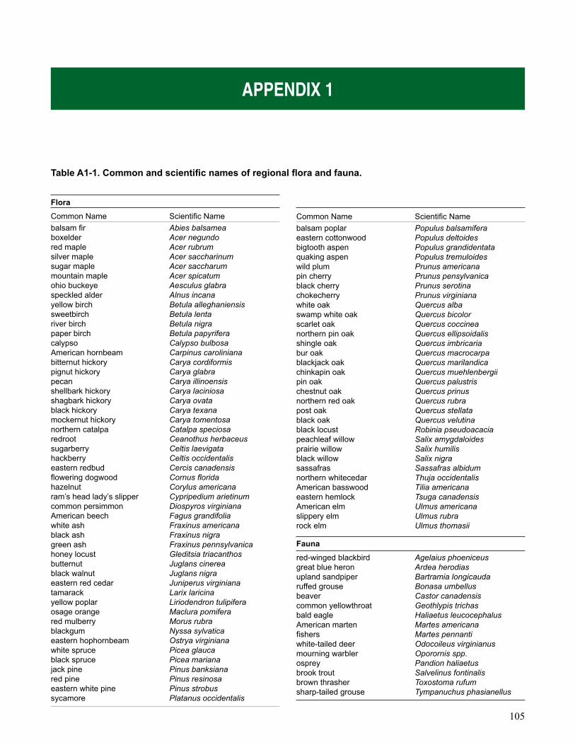
105
APPENDIX 1
Flora
Common Name Scientifi c Namebalsam fi r Abies balsameaboxelder Acer negundored maple Acer rubrumsilver maple Acer saccharinumsugar maple Acer saccharummountain maple Acer spicatumohio buckeye Aesculus glabraspeckled alder Alnus incanayellow birch Betula alleghaniensissweetbirch Betula lentariver birch Betula nigrapaper birch Betula papyriferacalypso Calypso bulbosaAmerican hornbeam Carpinus carolinianabitternut hickory Carya cordiformispignut hickory Carya glabrapecan Carya illinoensisshellbark hickory Carya laciniosashagbark hickory Carya ovatablack hickory Carya texanamockernut hickory Carya tomentosanorthern catalpa Catalpa speciosaredroot Ceanothus herbaceussugarberry Celtis laevigatahackberry Celtis occidentaliseastern redbud Cercis canadensisfl owering dogwood Cornus fl oridahazelnut Corylus americanaram’s head lady’s slipper Cypripedium arietinumcommon persimmon Diospyros virginianaAmerican beech Fagus grandifoliawhite ash Fraxinus americanablack ash Fraxinus nigragreen ash Fraxinus pennsylvanicahoney locust Gleditsia triacanthosbutternut Juglans cinereablack walnut Juglans nigraeastern red cedar Juniperus virginianatamarack Larix laricinayellow poplar Liriodendron tulipiferaosage orange Maclura pomiferared mulberry Morus rubrablackgum Nyssa sylvaticaeastern hophornbeam Ostrya virginianawhite spruce Picea glaucablack spruce Picea marianajack pine Pinus banksianared pine Pinus resinosaeastern white pine Pinus strobussycamore Platanus occidentalis
Common Name Scientifi c Namebalsam poplar Populus balsamiferaeastern cottonwood Populus deltoidesbigtooth aspen Populus grandidentataquaking aspen Populus tremuloideswild plum Prunus americanapin cherry Prunus pensylvanicablack cherry Prunus serotinachokecherry Prunus virginianawhite oak Quercus albaswamp white oak Quercus bicolorscarlet oak Quercus coccineanorthern pin oak Quercus ellipsoidalisshingle oak Quercus imbricariabur oak Quercus macrocarpablackjack oak Quercus marilandicachinkapin oak Quercus muehlenbergiipin oak Quercus palustrischestnut oak Quercus prinusnorthern red oak Quercus rubrapost oak Quercus stellatablack oak Quercus velutinablack locust Robinia pseudoacaciapeachleaf willow Salix amygdaloidesprairie willow Salix humilisblack willow Salix nigrasassafras Sassafras albidumnorthern whitecedar Thuja occidentalisAmerican basswood Tilia americanaeastern hemlock Tsuga canadensisAmerican elm Ulmus americanaslippery elm Ulmus rubrarock elm Ulmus thomasii
Fauna
red-winged blackbird Agelaius phoeniceusgreat blue heron Ardea herodiasupland sandpiper Bartramia longicaudaruffed grouse Bonasa umbellusbeaver Castor canadensiscommon yellowthroat Geothlypis trichasbald eagle Haliaetus leucocephalusAmerican marten Martes americanafi shers Martes pennantiwhite-tailed deer Odocoileus virginianusmourning warbler Oporornis spp.osprey Pandion haliaetusbrook trout Salvelinus fontinalisbrown thrasher Toxostoma rufumsharp-tailed grouse Tympanuchus phasianellus
Table A1-1. Common and scientifi c names of regional fl ora and fauna.
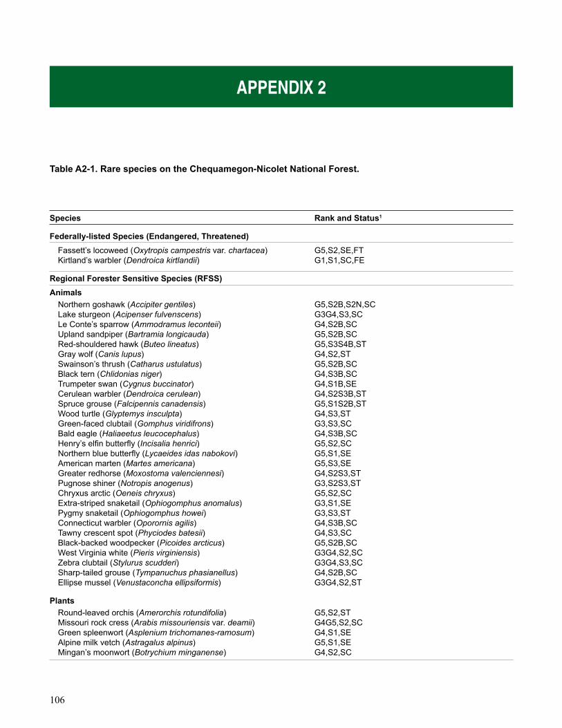
106
APPENDIX 2
Species Rank and Status1
Federally-listed Species (Endangered, Threatened)Fassett’s locoweed (Oxytropis campestris var. chartacea) G5,S2,SE,FTKirtland’s warbler (Dendroica kirtlandii) G1,S1,SC,FE
Regional Forester Sensitive Species (RFSS)Animals
Northern goshawk (Accipiter gentiles) G5,S2B,S2N,SCLake sturgeon (Acipenser fulvenscens) G3G4,S3,SCLe Conte’s sparrow (Ammodramus leconteii) G4,S2B,SCUpland sandpiper (Bartramia longicauda) G5,S2B,SCRed-shouldered hawk (Buteo lineatus) G5,S3S4B,STGray wolf (Canis lupus) G4,S2,STSwainson’s thrush (Catharus ustulatus) G5,S2B,SCBlack tern (Chlidonias niger) G4,S3B,SCTrumpeter swan (Cygnus buccinator) G4,S1B,SECerulean warbler (Dendroica cerulean) G4,S2S3B,STSpruce grouse (Falcipennis canadensis) G5,S1S2B,STWood turtle (Glyptemys insculpta) G4,S3,STGreen-faced clubtail (Gomphus viridifrons) G3,S3,SCBald eagle (Haliaeetus leucocephalus) G4,S3B,SCHenry’s elfi n butterfl y (Incisalia henrici) G5,S2,SCNorthern blue butterfl y (Lycaeides idas nabokovi) G5,S1,SEAmerican marten (Martes americana) G5,S3,SEGreater redhorse (Moxostoma valenciennesi) G4,S2S3,STPugnose shiner (Notropis anogenus) G3,S2S3,STChryxus arctic (Oeneis chryxus) G5,S2,SCExtra-striped snaketail (Ophiogomphus anomalus) G3,S1,SEPygmy snaketail (Ophiogomphus howei) G3,S3,STConnecticut warbler (Oporornis agilis) G4,S3B,SCTawny crescent spot (Phyciodes batesii) G4,S3,SCBlack-backed woodpecker (Picoides arcticus) G5,S2B,SCWest Virginia white (Pieris virginiensis) G3G4,S2,SCZebra clubtail (Stylurus scudderi) G3G4,S3,SCSharp-tailed grouse (Tympanuchus phasianellus) G4,S2B,SCEllipse mussel (Venustaconcha ellipsiformis) G3G4,S2,ST
PlantsRound-leaved orchis (Amerorchis rotundifolia) G5,S2,STMissouri rock cress (Arabis missouriensis var. deamii) G4G5,S2,SCGreen spleenwort (Asplenium trichomanes-ramosum) G4,S1,SEAlpine milk vetch (Astragalus alpinus) G5,S1,SEMingan’s moonwort (Botrychium minganense) G4,S2,SC
Table A2-1. Rare species on the Chequamegon-Nicolet National Forest.
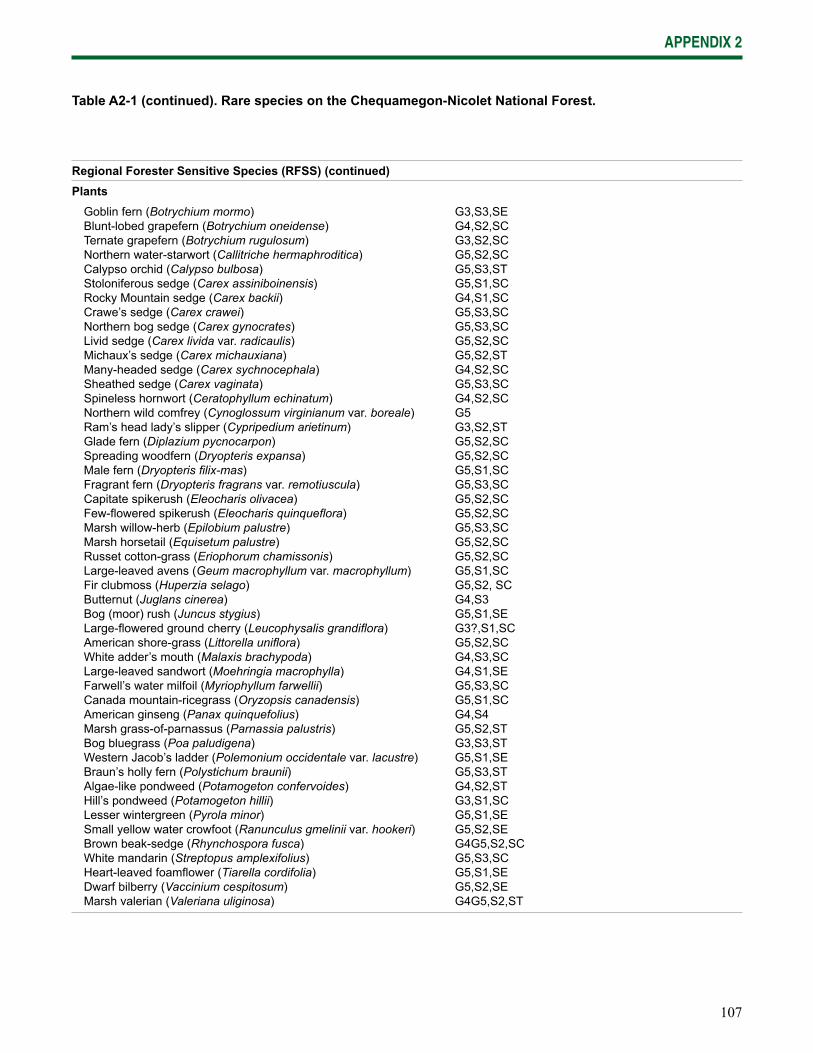
107
APPENDIX 2
Regional Forester Sensitive Species (RFSS) (continued)Plants
Goblin fern (Botrychium mormo) G3,S3,SEBlunt-lobed grapefern (Botrychium oneidense) G4,S2,SCTernate grapefern (Botrychium rugulosum) G3,S2,SCNorthern water-starwort (Callitriche hermaphroditica) G5,S2,SCCalypso orchid (Calypso bulbosa) G5,S3,STStoloniferous sedge (Carex assiniboinensis) G5,S1,SCRocky Mountain sedge (Carex backii) G4,S1,SCCrawe’s sedge (Carex crawei) G5,S3,SCNorthern bog sedge (Carex gynocrates) G5,S3,SCLivid sedge (Carex livida var. radicaulis) G5,S2,SCMichaux’s sedge (Carex michauxiana) G5,S2,STMany-headed sedge (Carex sychnocephala) G4,S2,SCSheathed sedge (Carex vaginata) G5,S3,SCSpineless hornwort (Ceratophyllum echinatum) G4,S2,SCNorthern wild comfrey (Cynoglossum virginianum var. boreale) G5Ram’s head lady’s slipper (Cypripedium arietinum) G3,S2,STGlade fern (Diplazium pycnocarpon) G5,S2,SCSpreading woodfern (Dryopteris expansa) G5,S2,SCMale fern (Dryopteris fi lix-mas) G5,S1,SCFragrant fern (Dryopteris fragrans var. remotiuscula) G5,S3,SCCapitate spikerush (Eleocharis olivacea) G5,S2,SCFew-fl owered spikerush (Eleocharis quinquefl ora) G5,S2,SCMarsh willow-herb (Epilobium palustre) G5,S3,SCMarsh horsetail (Equisetum palustre) G5,S2,SCRusset cotton-grass (Eriophorum chamissonis) G5,S2,SCLarge-leaved avens (Geum macrophyllum var. macrophyllum) G5,S1,SCFir clubmoss (Huperzia selago) G5,S2, SCButternut (Juglans cinerea) G4,S3Bog (moor) rush (Juncus stygius) G5,S1,SELarge-fl owered ground cherry (Leucophysalis grandifl ora) G3?,S1,SCAmerican shore-grass (Littorella unifl ora) G5,S2,SCWhite adder’s mouth (Malaxis brachypoda) G4,S3,SCLarge-leaved sandwort (Moehringia macrophylla) G4,S1,SEFarwell’s water milfoil (Myriophyllum farwellii) G5,S3,SCCanada mountain-ricegrass (Oryzopsis canadensis) G5,S1,SCAmerican ginseng (Panax quinquefolius) G4,S4Marsh grass-of-parnassus (Parnassia palustris) G5,S2,STBog bluegrass (Poa paludigena) G3,S3,STWestern Jacob’s ladder (Polemonium occidentale var. lacustre) G5,S1,SEBraun’s holly fern (Polystichum braunii) G5,S3,STAlgae-like pondweed (Potamogeton confervoides) G4,S2,STHill’s pondweed (Potamogeton hillii) G3,S1,SCLesser wintergreen (Pyrola minor) G5,S1,SESmall yellow water crowfoot (Ranunculus gmelinii var. hookeri) G5,S2,SEBrown beak-sedge (Rhynchospora fusca) G4G5,S2,SCWhite mandarin (Streptopus amplexifolius) G5,S3,SCHeart-leaved foamfl ower (Tiarella cordifolia) G5,S1,SEDwarf bilberry (Vaccinium cespitosum) G5,S2,SEMarsh valerian (Valeriana uliginosa) G4G5,S2,ST
Table A2-1 (continued). Rare species on the Chequamegon-Nicolet National Forest.
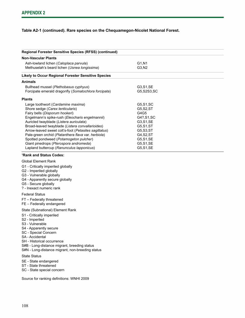
108
APPENDIX 2
Table A2-1 (continued). Rare species on the Chequamegon-Nicolet National Forest.
Regional Forester Sensitive Species (RFSS) (continued)Non-Vascular Plants
Ash-lowland lichen (Caloplaca parvula) G1,N1Methuselah’s beard lichen (Usnea longissima) G3,N2
Likely to Occur Regional Forester Sensitive SpeciesAnimals
Bullhead mussel (Plethobasus cyphyus) G3,S1,SEForcipate emerald dragonfl y (Somatochlora forcipata) G5,S2S3,SC
PlantsLarge toothwort (Cardamine maxima) G5,S1,SCShore sedge (Carex lenticularis) G5,S2,STFairy bells (Disporum hookeri) G4G5Engelmann’s spike-rush (Eleocharis engelmannii) G4?,S1,SCAuricled twayblade (Listera auriculata) G3,S1,SEBroad-leaved twayblade (Listera convallarioides) G5,S1,STArrow-leaved sweet colt’s-foot (Petasites sagittatus) G5,S3,STPale-green orchid (Platanthera fl ava var. herbiola) G4,S2,STSpotted pondweed (Potamogeton pulcher) G5,S1,SEGiant pinedrops (Pterospora andromeda) G5,S1,SELapland buttercup (Ranunculus lapponicus) G5,S1,SE
1Rank and Status Codes:Global Element RankG1 - Critically imperiled globallyG2 - Imperiled globallyG3 - Vulnerable globallyG4 - Apparently secure globally G5 - Secure globally? - Inexact numeric rank
Federal StatusFT – Federally threatenedFE – Federally endangered
State (Subnational) Element RankS1 - Critically imperiledS2 - ImperiledS3 - VulnerableS4 - Apparently secureSC - Special ConcernSA - AccidentalSH - Historical occurrenceS#B - Long-distance migrant, breeding statusS#N - Long-distance migrant, non-breeding status
State StatusSE - State endangeredST - State threatenedSC - State special concern
Source for ranking defi nitions: WNHI 2009
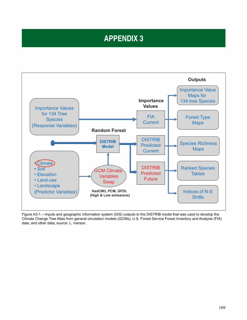
109
APPENDIX 3
Figure A3-1.—Inputs and geographic information system (GIS) outputs to the DISTRIB model that was used to develop the Climate Change Tree Atlas from general circulation models (GCMs), U.S. Forest Service Forest Inventory and Analysis (FIA) data, and other data; source: L. Iverson.
Outputs
Importance ValueMaps for
134 tree SpeciesImportance
Outputs
Importance Valuesfor 134 Tree
Species(Response Variables)
FIACurrent
p
Forest TypeMaps
pValues
(Response Variables)
DISTRIBModel
DISTRIBPredicted Species Richness
Maps
Random Forest
• Climate• Soil
Current
Ranked Species
Maps
DISTRIBGCM Climate• Elevation• Land-use• Landscape(Predictor Variables)
Tables
Indices of N-S
PredictedFuture
HadCM3, PCM, GFDL
GCM ClimateVariables
Swap
(Predictor Variables)Shifts(High & Low emissions)
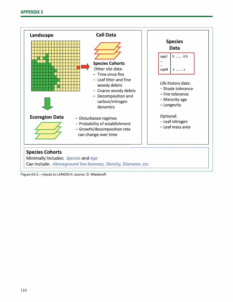
110
APPENDIX 3
Figure A3-2.—Inputs to LANDIS-II; source: D. Mladenoff.
111
APPENDIX 4. TREE SPECIES VULNERABILITY WITHIN NORTHERN WISCONSIN FORESTS TO CLIMATE CHANGES1
In this Appendix, we go into far more technical detail than Chapter 4 about the modeling methods and the results of this assessment. Becoming familiar with the methodology and rating schemes will allow readers to compare species’ potential to change under various scenarios of climate change.
Wisconsin has been realizing a recent warming, a trend that is projected to increase at a level that is being determined largely by human decisions and actions. A warming climate will impact forest ecosystems and the humans who work and play in them. Climate change is expected to shift the suitable habitat for tree species generally northward. Obviously, individual trees cannot get up and walk to more suitable habitats, so the trees currently or potentially in habitats that become increasingly unsuitable for them would become stressed, resulting in increased mortality, declining regeneration success, and dwindling populations. Catastrophic events, such as severe storms or fi res, are also more probable under most scenarios of climate change. Such events could precipitate rapid species turnover against the stressed trees in favor of the more suitable species. The increasing stress would also make some species more susceptible to other stressors, including droughts, fl oods, pathogens, insects, invasive plants and animals, and atmospheric deposition. Tree mortality could rise due to these secondary impacts, but it may be diffi cult to attribute the changes directly to a changing climate.
Conversely, habitat that becomes less suitable for one suite of species would likely become more suitable for
1 Louis Iverson, Anantha Prasad, Stephen Matthews, and Matthew Peters, Northern Research Station, Delaware, OH
others. Some of those species are already present in northern (or southern) Wisconsin, and their numbers would likely increase as they experience greater regeneration success and survival. Some other species, which are presently growing far south, may have newly suitable growing conditions appear in northern Wisconsin. Whether species would become established in these newly suitable areas depends on natural or artifi cial migration rates and the species’ specifi c requirements for establishment and growth. Healthy debate and research is needed to evaluate whether assisted migration for newly suitable species should be pursued, and if so, how it can be effectively done and where (Hoegh-Guldberg et al. 2008, Vitt et al. 2010).
Climate change is also likely to change the productivity of the forest ecosystems. If species become stressed because they are no longer well suited to their climate, their growth rates will likely decline. However, the warmer temperatures, longer growing seasons, and higher levels of carbon dioxide will compensate in some ways and lead to faster growth rates for some species.
The ranges of tree species in eastern North America have generally shifted northward as the climate has warmed over the past 14,000+ years since the last ice age (Davis 1981, Delcourt and Delcourt 1981, Webb et al. 1987). Evidence is mounting that tree species, along with many other organisms, are continuing this northward movement, some at very high rates (Hoegh-Guldberg et al. 2008). Evidence is growing of wide-spread tree mortality that can be attributed to drier and hotter conditions, often predisposing forests to insect pest outbreaks, such as the mountain pine beetle in western North America (Allen et al. 2010).
112
APPENDIX 4
Habitats for individual species have always, and will continue to, shift independently and at different rates, resulting in changing forest community compositions over time (Webb 1992). Such shifts are likely to occur in the coming decades in Wisconsin, so that suitable habitat will decline to different degrees among some species, while others will increase to various degrees. Some species will retain the same habitat, while others could completely disappear from northern Wisconsin. While it is likely that habitat will become suitable for some species not currently found in the State, it is less clear how rapidly—or even whether—those species will migrate into the region without active human intervention (Higgins and Harte 2006). Studies on six eastern United States species showed that, at the estimated maximum migration rate for the Holocene period (50 km per century in fully forested conditions, Davis 1981), less than 15 percent of the newly suitable habitat has even a small possibility of being colonized within 100 years (Iverson et al. 2004).
The relatively rapid nature of the projected climate shifts, along with the limits on the rate at which trees can migrate over a landscape, especially in the current and future fragmented state of forests, constrain the rate of ‘natural’ migration. We are currently incorporating this constraint for numerous tree species with a spatially explicit cellular model (SHIFT) that calculates colonization probabilities for each cell based on habitat quality, abundance of the species, and distance between colonized and uncolonized cells.
The work presented here is based on modeling the primary individual tree species of northern Wisconsin. We briefl y describe the methods we used and then present an evaluation of potential tree species changes, along with several other interpretive measures that complement the models, to assist in further evaluation of vulnerabilities and potential management options.
Methods
The region of study is approximately the northern third of Wisconsin, defi ned by Ecological Province 212 (Laurentian Mixed Forest Province) that occurs in Wisconsin, hereafter referred to as Wisconsin 212 (Introduction, Fig. 1). The Chequamegon-Nicolet National Forest (CNNF) is in this area, intermixed with much State, local, and private forests. These forests are rather fragmented and young, as the area was mostly cutover prior to the CNNF beginning forest management in the early 1930s.
Each species is modeled separately using a statistical approach based on where the species now exists in relation to many soil, climate, and landscape features. For species information on a total of 134 tree species, we used U.S. Forest Service Forest Inventory and Analysis (FIA) data to build importance value estimates for each species. We use 38 environmental variables—7 climate, 9 soil-class, 12 soil-characteristic, 5 landscape and fragmentation, and 5 elevation variables—to model current species abundance with respect to the environment. Then, current climate variables (1960 to 1990) are swapped with the future climates (~2070 to 2100) according to several global circulation models (GCMs) and emissions scenarios. We used two emissions scenarios developed for the Intergovernmental Panel on Climate Change (IPCC): a high level of emissions (A1FI) that assumes a continued high rate of fossil fuel emissions to 2050, and a lower emissions scenario (B2) that assumes a rapid conversion to conservation of energy and reduced reliance on fossil fuels (Nakicenovic et al. 2000).
The scenarios are also based on the output from three different GCMs: the HadleyCM3 model (Pope 2000), the GFDL or Geophysical Fluid Dynamics Laboratory model (Delworth et al. 2006), and the PCM or Parallel Climate Model (Washington et al. 2000). For reporting, we present the HadleyCM3 model projections under the high emissions scenario (HadHi)
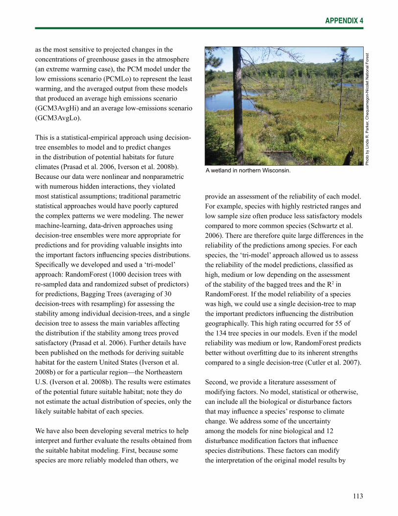
113
APPENDIX 4
as the most sensitive to projected changes in the concentrations of greenhouse gases in the atmosphere (an extreme warming case), the PCM model under the low emissions scenario (PCMLo) to represent the least warming, and the averaged output from these models that produced an average high emissions scenario (GCM3AvgHi) and an average low-emissions scenario (GCM3AvgLo).
This is a statistical-empirical approach using decision-tree ensembles to model and to predict changes in the distribution of potential habitats for future climates (Prasad et al. 2006, Iverson et al. 2008b). Because our data were nonlinear and nonparametric with numerous hidden interactions, they violated most statistical assumptions; traditional parametric statistical approaches would have poorly captured the complex patterns we were modeling. The newer machine-learning, data-driven approaches using decision-tree ensembles were more appropriate for predictions and for providing valuable insights into the important factors infl uencing species distributions. Specifi cally we developed and used a ‘tri-model’ approach: RandomForest (1000 decision trees with re-sampled data and randomized subset of predictors) for predictions, Bagging Trees (averaging of 30 decision-trees with resampling) for assessing the stability among individual decision-trees, and a single decision tree to assess the main variables affecting the distribution if the stability among trees proved satisfactory (Prasad et al. 2006). Further details have been published on the methods for deriving suitable habitat for the eastern United States (Iverson et al. 2008b) or for a particular region—the Northeastern U.S. (Iverson et al. 2008b). The results were estimates of the potential future suitable habitat; note they do not estimate the actual distribution of species, only the likely suitable habitat of each species.
We have also been developing several metrics to help interpret and further evaluate the results obtained from the suitable habitat modeling. First, because some species are more reliably modeled than others, we
provide an assessment of the reliability of each model. For example, species with highly restricted ranges and low sample size often produce less satisfactory models compared to more common species (Schwartz et al. 2006). There are therefore quite large differences in the reliability of the predictions among species. For each species, the ‘tri-model’ approach allowed us to assess the reliability of the model predictions, classifi ed as high, medium or low depending on the assessment of the stability of the bagged trees and the R2 in RandomForest. If the model reliability of a species was high, we could use a single decision-tree to map the important predictors infl uencing the distribution geographically. This high rating occurred for 55 of the 134 tree species in our models. Even if the model reliability was medium or low, RandomForest predicts better without overfi tting due to its inherent strengths compared to a single decision-tree (Cutler et al. 2007).
Second, we provide a literature assessment of modifying factors. No model, statistical or otherwise, can include all the biological or disturbance factors that may infl uence a species’ response to climate change. We address some of the uncertainty among the models for nine biological and 12 disturbance modifi cation factors that infl uence species distributions. These factors can modify the interpretation of the original model results by
A wetland in northern Wisconsin.
Pho
to b
y Li
nda
R. P
arke
r, C
hequ
ameg
on-N
icol
et N
atio
nal F
ores
t
114
APPENDIX 4
increasing or decreasing potential future importance of a species. Each species is given a default score based on the literature, and can be changed by managers as they consider local conditions for each of the factors. With knowledge of site-specifi c processes, managers may be better suited to interpret the models after considering the modifi cation factors. They can then use these factors to modify the interpretation of the potential suitable habitat models. The goal of this effort is to provide information on the distribution of species under climate change that accounts for the natural processes that infl uence the fi nal distribution. This approach encourages decision makers to be actively involved in managing tree habitats under projected future climatic conditions.
Another important consideration for model interpretation is to identify the predictor variables that have the most infl uence on the species, and whether they are occurring at the broadest extent of the species range or exerting infl uence on species at a more local scale. This not only helps to understand how the models are working but also provides insights to managers on the factors that control species distributions. Therefore, we partition the variable importance scores into the two scale categories based on the pattern of variable node location within the intermediate steps of the RandomForest algorithm. To statistically distinguish the very important biological question of whether a variable is only marginally important at the broadest extent vs. very important at a local scale (these two situations could have very similar variable importance scores), we examine the RandomForest ensemble structure for an assessment of where (what node) and with what strength these variables are entering the model. The node location is summarized over all trees and for each variable where it occurs. Then we weight the position by the frequency of occupancies at the location to determine an average fi rst position of the variable. The weighted node location in many ways represents an inverse relationship to the variable importance value; when these two metrics are combined it is possible to
evaluate the relative contribution of the variables to the initial splits of the data (thus refl ecting more regional partitioning). This allows us to partition the total variable importance (weighted by the number of variables in a class) for these regional variables into climate, soil, elevation, and landscape components. The second group of variables is then designated as being beyond the fi rst cut, up to the median weighted node location or where they most frequently occur no further then the 15th node split. These variables represent the more locally infl uencing variables.
For those species that are predicted to have new suitable habitat appear in northern Wisconsin, we provide an assessment on how far each may have to travel to reach the southern border of Wisconsin 212. This entailed a statistical approximation of the current species boundary, followed by an estimation of the Euclidean distance to the nearest edge of the Wisconsin 212 boundary.
Each of 134 tree species was evaluated for presence in Wisconsin 212, either now or potentially in the future (with a few very minor and poorly modeled species eliminated). The above metrics were sorted into 3 to 5 classes, with a 0 class, 1 to 2 negative class, and 1 to 2 positive class (examples for Biological Factors: BF--, BF-, BF0, BF+, BF++; and for Model Reliability: MR-, MR0, MR+).
Finally, we are beginning to evaluate selected species for their potential migration from where they exist currently to where they may be able to colonize over the next 100 years. This helps us understand not only how the suitable habitat may move, but also how far the species may move across the fragmented habitats of southern Wisconsin. We calibrate movement at the approximate (generous) migration rate of 50 km per century, according to paleoecological data from the Holocene period (Davis 1981). Details of the method (although under revision now) are presented in several publications (Iverson and Schwartz 1999, Iverson et al. 2004, Schwartz et al. 2006).
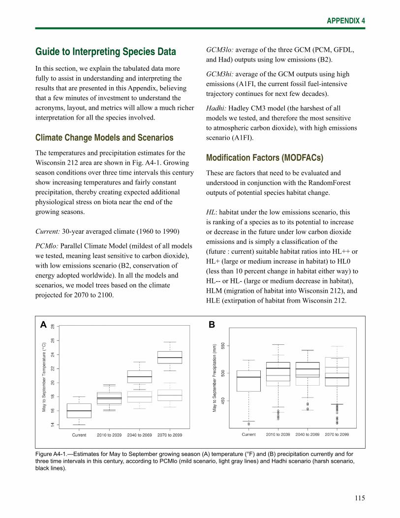
115
APPENDIX 4
Guide to Interpreting Species Data
In this section, we explain the tabulated data more fully to assist in understanding and interpreting the results that are presented in this Appendix, believing that a few minutes of investment to understand the acronyms, layout, and metrics will allow a much richer interpretation for all the species involved.
Climate Change Models and Scenarios
The temperatures and precipitation estimates for the Wisconsin 212 area are shown in Fig. A4-1. Growing season conditions over three time intervals this century show increasing temperatures and fairly constant precipitation, thereby creating expected additional physiological stress on biota near the end of the growing seasons.
Current: 30-year averaged climate (1960 to 1990)
PCMlo: Parallel Climate Model (mildest of all models we tested, meaning least sensitive to carbon dioxide), with low emissions scenario (B2, conservation of energy adopted worldwide). In all the models and scenarios, we model trees based on the climate projected for 2070 to 2100.
GCM3lo: average of the three GCM (PCM, GFDL, and Had) outputs using low emissions (B2).
GCM3hi: average of the GCM outputs using high emissions (A1FI, the current fossil fuel-intensive trajectory continues for next few decades).
Hadhi: Hadley CM3 model (the harshest of all models we tested, and therefore the most sensitive to atmospheric carbon dioxide), with high emissions scenario (A1FI).
Modifi cation Factors (MODFACs)
These are factors that need to be evaluated and understood in conjunction with the RandomForest outputs of potential species habitat change.
HL: habitat under the low emissions scenario, this is ranking of a species as to its potential to increase or decrease in the future under low carbon dioxide emissions and is simply a classifi cation of the (future : current) suitable habitat ratios into HL++ or HL+ (large or medium increase in habitat) to HL0 (less than 10 percent change in habitat either way) to HL-- or HL- (large or medium decrease in habitat), HLM (migration of habitat into Wisconsin 212), and HLE (extirpation of habitat from Wisconsin 212.
Figure A4-1.—Estimates for May to September growing season (A) temperature (°F) and (B) precipitation currently and for three time intervals in this century, according to PCMlo (mild scenario, light gray lines) and Hadhi scenario (harsh scenario, black lines).
A B
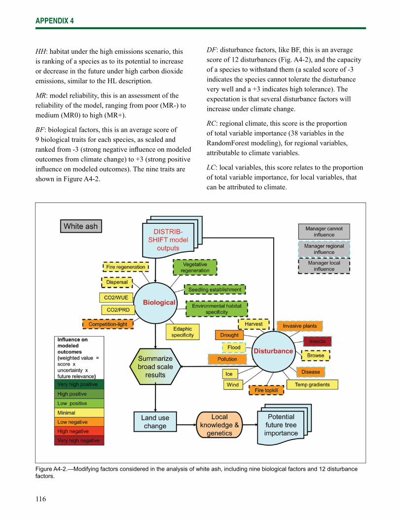
116
APPENDIX 4
HH: habitat under the high emissions scenario, this is ranking of a species as to its potential to increase or decrease in the future under high carbon dioxide emissions, similar to the HL description.
MR: model reliability, this is an assessment of the reliability of the model, ranging from poor (MR-) to medium (MR0) to high (MR+).
BF: biological factors, this is an average score of 9 biological traits for each species, as scaled and ranked from -3 (strong negative infl uence on modeled outcomes from climate change) to +3 (strong positive infl uence on modeled outcomes). The nine traits are shown in Figure A4-2.
DF: disturbance factors, like BF, this is an average score of 12 disturbances (Fig. A4-2), and the capacity of a species to withstand them (a scaled score of -3 indicates the species cannot tolerate the disturbance very well and a +3 indicates high tolerance). The expectation is that several disturbance factors will increase under climate change.
RC: regional climate, this score is the proportion of total variable importance (38 variables in the RandomForest modeling), for regional variables, attributable to climate variables.
LC: local variables, this score relates to the proportion of total variable importance, for local variables, that can be attributed to climate.
Figure A4-2.—Modifying factors considered in the analysis of white ash, including nine biological factors and 12 disturbance factors.
117
APPENDIX 4
MD: migration distance, this score only applies to species that currently do not exist in Wisconsin 212 but may have habitat appear there by 2100. The number following the MD is a rounded off Euclidian distance (nearest 100 km) from the current range boundary to the southern boundary of Wisconsin 212. NA (not available) indicates we cannot calculate the MD.
Occupancy
The total study area consists of 225 20 x 20 km cells within the Wisconsin 212 area that were modeled to be of suitable habitat for the species cells. Data are reported for Current, PCMlo, GCM3lo, GCM3hi, and Hadhi.
Area Weighted Importance Values (AWIV)
For each of the 225 cells in Wisconsin 212, the average importance value was calculated and then summed across all cells to obtain the area weighted importance value for each species, and for each scenario (Current, PCMlo, GCM3lo, GCM3hi, and Hadhi). Importance values are relative scores (ranging from 0 to 100) based on basal area and number of stems in inventory plots, with 100 indicating the presence of a only a single species. Theoretically, if only one species was found everywhere, the maximum AWIV would be calculated as: 100 importance value average x 225 cells = 22500. Of course in reality, no species comes anywhere close to this theoretical maximum.
Future: Current Ratios
The ratio of AWIV under a future climate scenario to current. Thus, a score >1 indicates an increase in overall suitable habitat in the future (~2100), whereas a score < 1 indicates a decrease.
Niche Plot Scores
We plotted the current annual temperature and precipitation profi les for the eastern United States and the current distribution (by importance value) for each species within this profi le. We also overplotted three polygons, with black representing the climate of Wisconsin 212 now, blue representing the future under the PCMlo mild scenario, and red representing the future under the Hadhi harsh scenario (Fig. A4-3). Thus, the niche plot gives a quick view of whether a species currently exists in analog climates in the United States and whether it will have similar temperature/precipitation habitat in the future in Wisconsin 212. Of course, this analysis does not account for the capacity to adapt to new conditions, or the genetic variations contained within the species. In Table A4-3, we have calculated the percentage of the three polygons that the species occupies, allowing a quick comparison of a species’ future versus current temperature/precipitation conditions in Wisconsin 212.
Change Class
Each of 73 species has been assigned to one of eight classes, based on vulnerability to potential change under climate change. These are the primary classes determined by the RandomForest model of potential change in suitable habitat. Within these classes, we also present an overall assessment of the MODFACs adjustment to ranking interpretations. Species Model ResultsOf 134 species modeled in the eastern United States, 73 were of interest for Wisconsin 212. Using the estimates of potential changes in suitable habitat, we sorted the species according to their potential to gain, lose, remain unchanged, or enter into Wisconsin 212 from outside. We classify them into eight classes of vulnerability to climate change, ranging from most vulnerable to least, followed by the number of species in each class:
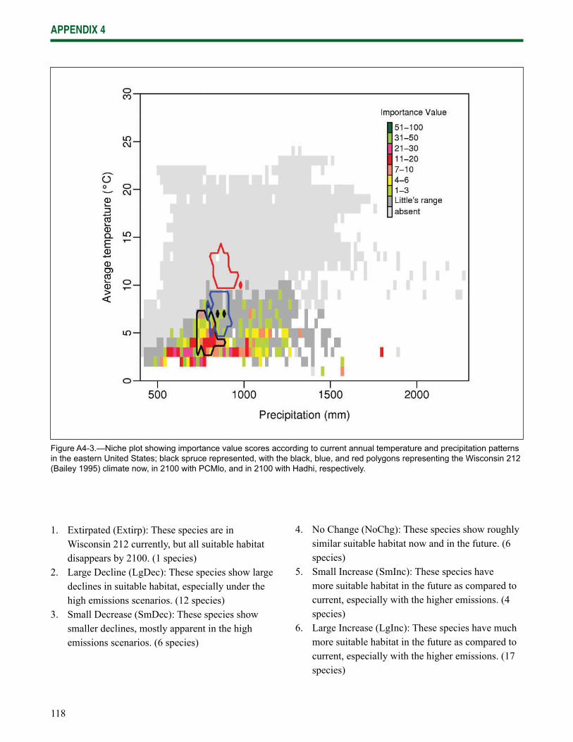
118
APPENDIX 4
Figure A4-3.—Niche plot showing importance value scores according to current annual temperature and precipitation patterns in the eastern United States; black spruce represented, with the black, blue, and red polygons representing the Wisconsin 212 (Bailey 1995) climate now, in 2100 with PCMlo, and in 2100 with Hadhi, respectively.
1. Extirpated (Extirp): These species are in Wisconsin 212 currently, but all suitable habitat disappears by 2100. (1 species)
2. Large Decline (LgDec): These species show large declines in suitable habitat, especially under the high emissions scenarios. (12 species)
3. Small Decrease (SmDec): These species show smaller declines, mostly apparent in the high emissions scenarios. (6 species)
4. No Change (NoChg): These species show roughly similar suitable habitat now and in the future. (6 species)
5. Small Increase (SmInc): These species have more suitable habitat in the future as compared to current, especially with the higher emissions. (4 species)
6. Large Increase (LgInc): These species have much more suitable habitat in the future as compared to current, especially with the higher emissions. (17 species)
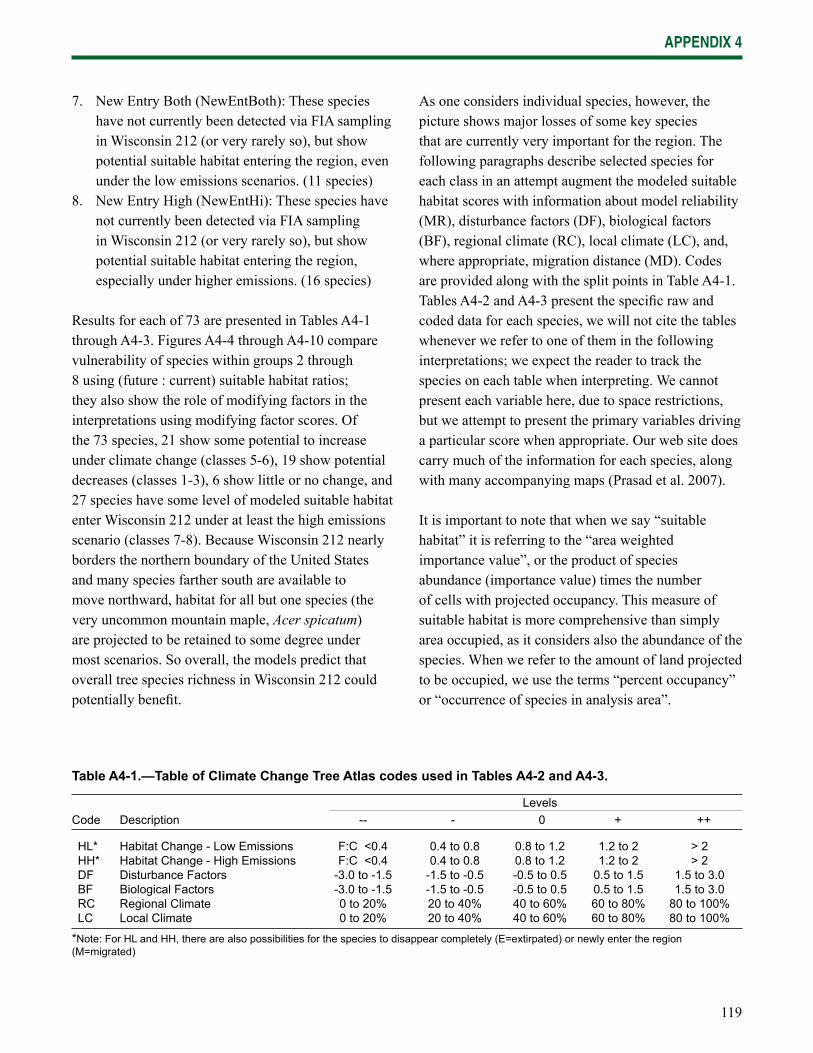
119
APPENDIX 4
7. New Entry Both (NewEntBoth): These species have not currently been detected via FIA sampling in Wisconsin 212 (or very rarely so), but show potential suitable habitat entering the region, even under the low emissions scenarios. (11 species)
8. New Entry High (NewEntHi): These species have not currently been detected via FIA sampling in Wisconsin 212 (or very rarely so), but show potential suitable habitat entering the region, especially under higher emissions. (16 species)
Results for each of 73 are presented in Tables A4-1 through A4-3. Figures A4-4 through A4-10 compare vulnerability of species within groups 2 through 8 using (future : current) suitable habitat ratios; they also show the role of modifying factors in the interpretations using modifying factor scores. Of the 73 species, 21 show some potential to increase under climate change (classes 5-6), 19 show potential decreases (classes 1-3), 6 show little or no change, and 27 species have some level of modeled suitable habitat enter Wisconsin 212 under at least the high emissions scenario (classes 7-8). Because Wisconsin 212 nearly borders the northern boundary of the United States and many species farther south are available to move northward, habitat for all but one species (the very uncommon mountain maple, Acer spicatum) are projected to be retained to some degree under most scenarios. So overall, the models predict that overall tree species richness in Wisconsin 212 could potentially benefi t.
As one considers individual species, however, the picture shows major losses of some key species that are currently very important for the region. The following paragraphs describe selected species for each class in an attempt augment the modeled suitable habitat scores with information about model reliability (MR), disturbance factors (DF), biological factors (BF), regional climate (RC), local climate (LC), and, where appropriate, migration distance (MD). Codes are provided along with the split points in Table A4-1. Tables A4-2 and A4-3 present the specifi c raw and coded data for each species, we will not cite the tables whenever we refer to one of them in the following interpretations; we expect the reader to track the species on each table when interpreting. We cannot present each variable here, due to space restrictions, but we attempt to present the primary variables driving a particular score when appropriate. Our web site does carry much of the information for each species, along with many accompanying maps (Prasad et al. 2007).
It is important to note that when we say “suitable habitat” it is referring to the “area weighted importance value”, or the product of species abundance (importance value) times the number of cells with projected occupancy. This measure of suitable habitat is more comprehensive than simply area occupied, as it considers also the abundance of the species. When we refer to the amount of land projected to be occupied, we use the terms “percent occupancy” or “occurrence of species in analysis area”.
Table A4-1.—Table of Climate Change Tree Atlas codes used in Tables A4-2 and A4-3.
LevelsCode Description -- - 0 + ++
HL* Habitat Change - Low Emissions F:C <0.4 0.4 to 0.8 0.8 to 1.2 1.2 to 2 > 2HH* Habitat Change - High Emissions F:C <0.4 0.4 to 0.8 0.8 to 1.2 1.2 to 2 > 2DF Disturbance Factors -3.0 to -1.5 -1.5 to -0.5 -0.5 to 0.5 0.5 to 1.5 1.5 to 3.0BF Biological Factors -3.0 to -1.5 -1.5 to -0.5 -0.5 to 0.5 0.5 to 1.5 1.5 to 3.0RC Regional Climate 0 to 20% 20 to 40% 40 to 60% 60 to 80% 80 to 100%LC Local Climate 0 to 20% 20 to 40% 40 to 60% 60 to 80% 80 to 100%
*Note: For HL and HH, there are also possibilities for the species to disappear completely (E=extirpated) or newly enter the region (M=migrated)
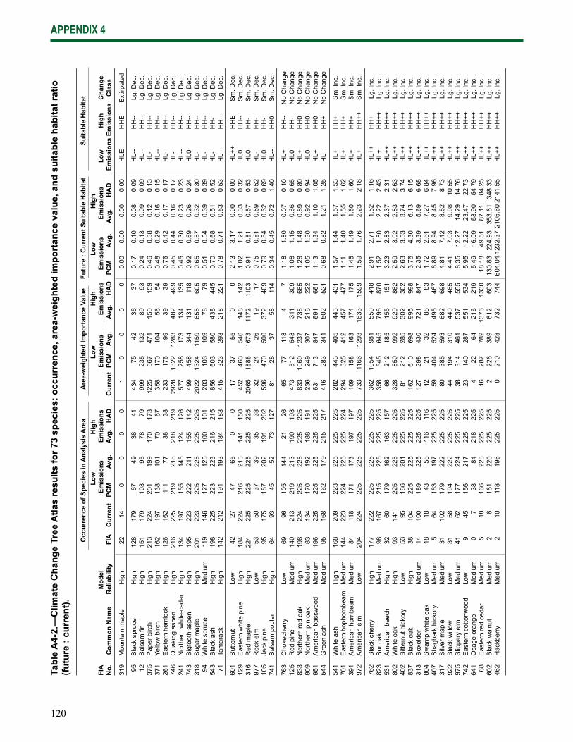
120
APPENDIX 4
319
Mou
ntai
n m
aple
H
igh
22
14
0 0
0 0
1 0
0 0
0 0.
00
0.00
0.
00
0.00
H
LE
HH
E
Ext
irpat
ed
95
Bla
ck s
pruc
e H
igh
128
179
67
49
38
41
434
75
42
36
37
0.17
0.
10
0.08
0.
09
HL-
- H
H--
Lg
. Dec
. 1
2 B
alsa
m fi
r H
igh
151
179
103
95
78
79
999
235
132
89
93
0.24
0.
13
0.09
0.
09
HL-
- H
H--
Lg
. Dec
.37
5 P
aper
birc
h H
igh
213
224
201
199
170
173
1225
56
7 47
1 15
0 15
9 0.
46
0.38
0.
12
0.13
H
L-
HH
--
Lg. D
ec.
371
Yello
w b
irch
Hig
h 16
2 19
7 13
8 10
1 70
67
35
8 17
0 10
4 56
54
0.
48
0.29
0.
16
0.15
H
L--
HH
--
Lg. D
ec.
261
Eas
tern
hem
lock
H
igh
126
162
111
77
38
38
233
176
99
39
39
0.76
0.
42
0.17
0.
17
HL-
H
H--
Lg
. Dec
.74
6 Q
uaki
ng a
spen
H
igh
216
225
219
218
218
219
2928
13
22
1283
48
2 49
9 0.
45
0.44
0.
16
0.17
H
L-
HH
--
Lg. D
ec.
241
Nor
ther
n w
hite
-ced
ar
Hig
h 13
4 19
7 15
5 14
5 12
4 12
6 57
7 25
8 17
3 13
4 13
5 0.
45
0.30
0.
23
0.23
H
L--
HH
--
Lg. D
ec.
743
Big
toot
h as
pen
Hig
h 19
5 22
3 22
2 21
1 15
5 14
2 49
9 45
8 34
4 13
1 11
8 0.
92
0.69
0.
26
0.24
H
L0
HH
--
Lg. D
ec.
318
Sug
ar m
aple
H
igh
201
223
225
225
225
225
2022
13
24
1159
65
5 60
5 0.
65
0.57
0.
32
0.30
H
L-
HH
--
Lg. D
ec.
94
Whi
te s
pruc
e M
ediu
m
119
146
127
125
100
101
203
103
109
78
79
0.51
0.
54
0.39
0.
39
HL-
H
H--
Lg
. Dec
.54
3 B
lack
ash
H
igh
198
225
223
223
216
215
856
603
580
438
445
0.70
0.
68
0.51
0.
52
HL-
H
H-
Lg. D
ec.
71
Tam
arac
k H
igh
142
212
191
193
184
183
415
323
293
218
221
0.78
0.
71
0.53
0.
53
HL-
H
H-
Lg. D
ec.
601
But
tern
ut
Low
42
27
47
66
0
0 17
37
55
0
0 2.
13
3.17
0.
00
0.00
H
L++
HH
E
Sm
. Dec
.12
9 E
aste
rn w
hite
pin
e H
igh
184
224
216
213
141
150
452
463
546
148
142
1.02
1.
21
0.33
0.
32
HL0
H
H--
S
m. D
ec.
316
Red
map
le
Hig
h 22
4 22
5 22
5 22
5 22
5 22
5 20
65
1888
16
73
1172
11
03
0.91
0.
81
0.57
0.
53
HL0
H
H-
Sm
. Dec
.97
7 R
ock
elm
Lo
w
53
50
37
39
35
38
32
24
26
19
17
0.75
0.
81
0.59
0.
52
HL-
H
H-
Sm
. Dec
.10
5 Ja
ck p
ine
Hig
h 95
17
5 18
7 20
2 19
1 20
2 59
6 47
0 50
0 37
2 40
9 0.
79
0.84
0.
62
0.69
H
L0
HH
- S
m. D
ec.
741
Bal
sam
pop
lar
Hig
h 64
93
45
52
73
12
7 81
28
37
58
11
4 0.
34
0.45
0.
72
1.40
H
L--
HH
0 S
m. D
ec.
763
Cho
kech
erry
Lo
w
69
96
105
144
21
26
65
77
118
4 7
1.18
1.
80
0.07
0.
10
HL+
H
H--
N
o C
hang
e12
5 R
ed p
ine
Med
ium
14
0 21
3 21
9 21
3 19
0 19
3 47
3 51
2 54
3 31
1 30
9 1.
08
1.15
0.
66
0.65
H
L0
HH
- N
o C
hang
e83
3 N
orth
ern
red
oak
Hig
h 19
8 22
4 22
5 22
5 22
5 22
5 83
3 10
69
1237
73
8 66
5 1.
28
1.48
0.
89
0.80
H
L+
HH
0 N
o C
hang
e80
9 N
orth
ern
pin
oak
Med
ium
83
13
4 17
0 19
2 18
8 19
1 23
6 24
9 30
7 21
6 22
2 1.
05
1.30
0.
92
0.94
H
L0
HH
0 N
o C
hang
e95
1 A
mer
ican
bas
swoo
d M
ediu
m
196
225
225
225
225
225
631
713
847
691
661
1.13
1.
34
1.10
1.
05
HL+
H
H0
No
Cha
nge
544
Gre
en a
sh
Med
ium
95
16
8 16
2 17
9 21
5 21
7 41
6 28
3 34
1 50
2 52
1 0.
68
0.82
1.
21
1.25
H
L-
HH
+ N
o C
hang
e
541
Whi
te a
sh
Hig
h 16
8 20
9 22
3 22
5 22
5 22
5 28
2 44
3 40
5 44
3 43
1 1.
57
1.44
1.
57
1.53
H
L+
HH
+ S
m. I
nc.
701
Eas
tern
hop
horn
beam
M
ediu
m
144
223
224
225
225
224
294
325
412
457
477
1.11
1.
40
1.55
1.
62
HL+
H
H+
Sm
. Inc
.39
1 A
mer
ican
hor
nbea
m
Med
ium
84
11
8 17
1 17
3 19
7 19
7 10
9 15
8 16
3 17
4 17
5 1.
45
1.49
1.
60
1.60
H
L+
HH
+ S
m. I
nc.
972
Am
eric
an e
lm
Low
20
4 22
4 22
5 22
5 22
5 22
5 73
3 11
66
1293
16
33
1599
1.
59
1.76
2.
23
2.18
H
L+
HH
++
Sm
. Inc
.
762
Bla
ck c
herr
y H
igh
177
222
225
225
225
225
362
1054
98
1 55
0 41
8 2.
91
2.71
1.
52
1.16
H
L++
HH
+ Lg
. Inc
.82
3 B
ur o
ak
Med
ium
98
16
7 21
5 22
5 22
5 22
5 35
8 54
5 64
5 79
6 87
0 1.
52
1.80
2.
22
2.43
H
L+
HH
++
Lg. I
nc.
531
Am
eric
an b
eech
H
igh
32
60
179
162
163
157
66
212
185
155
151
3.23
2.
83
2.37
2.
31
HL+
+ H
H++
Lg
. Inc
.80
2 W
hite
oak
H
igh
93
141
225
225
225
225
328
850
992
929
862
2.59
3.
02
2.83
2.
63
HL+
+ H
H++
Lg
. Inc
.40
2 B
itter
nut h
icko
ry
Low
53
95
16
6 20
1 22
5 22
5 81
21
2 28
5 30
2 30
2 2.
63
3.53
3.
74
3.74
H
L++
HH
++
Lg. I
nc.
837
Bla
ck o
ak
Hig
h 38
10
4 22
5 22
5 22
5 22
5 16
2 61
0 69
8 99
5 99
8 3.
76
4.30
6.
13
6.15
H
L++
HH
++
Lg. I
nc.
313
Box
elde
r M
ediu
m
14
100
189
225
225
225
127
298
430
721
847
2.35
3.
39
5.69
6.
68
HL+
+ H
H++
Lg
. Inc
.80
4 S
wam
p w
hite
oak
Lo
w
18
18
43
58
116
116
12
21
32
88
83
1.72
2.
61
7.27
6.
84
HL+
+ H
H++
Lg
. Inc
.40
7 S
hagb
ark
hick
ory
Med
ium
5
64
163
197
225
225
59
404
524
495
467
6.89
8.
94
8.45
7.
96
HL+
+ H
H++
Lg
. Inc
.31
7 S
ilver
map
le
Med
ium
31
10
2 17
9 22
2 22
5 22
5 80
38
5 59
3 68
2 69
8 4.
81
7.42
8.
52
8.73
H
L++
HH
++
Lg. I
nc.
922
Bla
ck w
illow
Lo
w
31
58
194
222
225
225
44
194
310
440
465
4.41
7.
03
9.98
10
.55
HL+
+ H
H++
Lg
. Inc
.97
5 S
lippe
ry e
lm
Med
ium
41
62
17
7 22
4 22
5 22
5 38
31
4 46
1 53
7 55
5 8.
35
12.2
7 14
.29
14.7
6 H
L++
HH
++
Lg. I
nc.
742
Eas
tern
cot
tonw
ood
Low
9
45
156
217
225
225
23
140
287
551
534
5.95
12
.22
23.4
7 22
.73
HL+
+ H
H++
Lg
. Inc
.64
1 O
sage
ora
nge
Med
ium
0
7 38
84
21
8 22
5 4
22
64
216
219
5.49
16
.09
53.9
0 54
.79
HL+
+ H
H++
Lg
. Inc
. 6
8 E
aste
rn re
d ce
dar
Med
ium
5
18
166
223
225
225
16
287
782
1376
13
30
18.1
8 49
.51
87.1
1 84
.25
HL+
+ H
H++
Lg
. Inc
.60
2 B
lack
wal
nut
Med
ium
2
8 16
1 22
0 22
5 22
5 2
226
389
612
603
130.
83
224.
93
353.
61
348.
33
HL+
+ H
H++
Lg
. Inc
.46
2 H
ackb
erry
M
ediu
m
2 10
11
8 19
6 22
5 22
5 0
210
428
732
744
604.
04 1
232.
37 2
105.
60 2
141.
55
HL+
+ H
H++
Lg
. Inc
.
Tabl
e A
4-2.
—C
limat
e C
hang
e Tr
ee A
tlas
resu
lts fo
r 73
spec
ies:
occ
urre
nce,
are
a-w
eigh
ted
impo
rtan
ce v
alue
, and
sui
tabl
e ha
bita
t rat
io
(futu
re :
curr
ent).
O
ccur
renc
e of
Spe
cies
in A
naly
sis
Are
a A
rea-
wei
ghte
d Im
port
ance
Val
ue
Futu
re :
Cur
rent
Sui
tabl
e H
abita
t Su
itabl
e H
abita
t
Low
H
igh
Low
H
igh
Low
H
igh
FIA
M
odel
Em
issi
ons
Emis
sion
s Em
issi
ons
Emis
sion
s Em
issi
ons
Emis
sion
s Lo
w
Hig
h C
hang
eN
o.
Com
mon
Nam
e R
elia
bilit
y FI
A C
urre
nt
PCM
Av
g.
Avg.
H
AD
C
urre
nt P
CM
Av
g.
Avg.
H
AD
PC
M
Avg.
Av
g.
HA
D
Emis
sion
s Em
issi
ons
Cla
ss
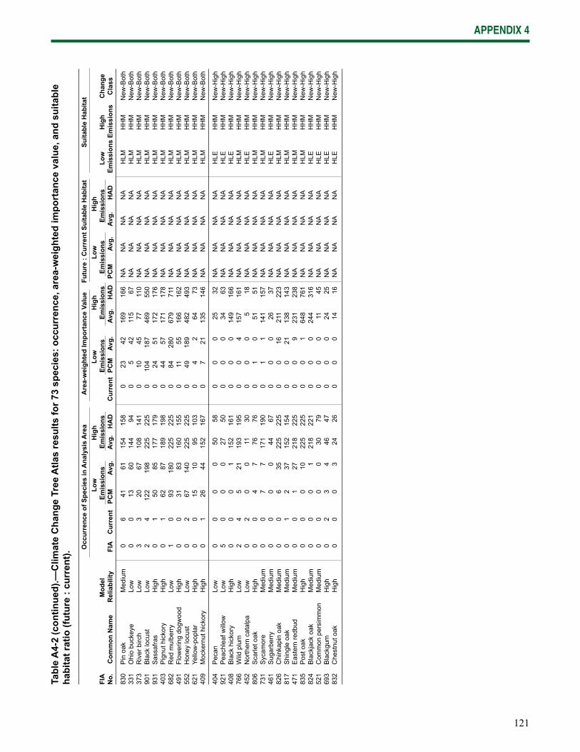
121
APPENDIX 4
830
Pin
oak
M
ediu
m
0 6
41
61
154
158
0 23
42
16
9 16
6 N
A N
A N
A N
A H
LM
HH
M
New
-Bot
h33
1 O
hio
buck
eye
Low
0
0 13
60
14
4 94
0
5 42
11
5 67
N
A N
A N
A N
A H
LM
HH
M
New
-Bot
h37
3 R
iver
birc
h Lo
w
3 3
20
67
108
141
0 10
45
77
11
0 N
A N
A N
A N
A H
LM
HH
M
New
-Bot
h90
1 B
lack
locu
st
Low
2
4 12
2 19
8 22
5 22
5 0
104
187
469
550
NA
NA
NA
NA
HLM
H
HM
N
ew-B
oth
931
Sas
safra
s H
igh
0 1
50
85
177
179
0 24
51
17
2 17
6 N
A N
A N
A N
A H
LM
HH
M
New
-Bot
h40
3 P
ignu
t hic
kory
H
igh
0 1
62
87
189
198
0 44
57
17
1 17
8 N
A N
A N
A N
A H
LM
HH
M
New
-Bot
h68
2 R
ed m
ulbe
rry
Low
1
0 93
18
0 22
5 22
5 0
84
280
679
711
NA
NA
NA
NA
HLM
H
HM
N
ew-B
oth
491
Flow
erin
g do
gwoo
d H
igh
0 0
31
83
160
155
0 11
55
16
6 16
2 N
A N
A N
A N
A H
LM
HH
M
New
-Bot
h55
2 H
oney
locu
st
Low
0
2 67
14
0 22
5 22
5 0
49
189
482
493
NA
NA
NA
NA
HLM
H
HM
N
ew-B
oth
621
Yello
w-p
opla
r H
igh
0 0
15
10
95
103
0 4
2 64
73
N
A N
A N
A N
A H
LM
HH
M
New
-Bot
h40
9 M
ocke
rnut
hic
kory
H
igh
0 1
26
44
152
167
0 7
21
135
146
NA
NA
NA
NA
HLM
H
HM
N
ew-B
oth
404
Pec
an
Low
0
0 0
0 50
58
0
0 0
25
32
NA
NA
NA
NA
HLE
H
HM
N
ew-H
igh
921
Pea
chle
af w
illow
Lo
w
5 0
0 0
27
50
0 0
0 34
63
N
A N
A N
A N
A H
LE
HH
M
New
-Hig
h40
8 B
lack
hic
kory
H
igh
0 0
0 1
152
161
0 0
0 14
9 16
6 N
A N
A N
A N
A H
LE
HH
M
New
-Hig
h76
6 W
ild p
lum
Lo
w
2 4
5 21
19
3 19
5 0
0 4
157
161
NA
NA
NA
NA
HLM
H
HM
N
ew-H
igh
452
Nor
ther
n ca
talp
a Lo
w
0 2
0 0
11
30
0 0
0 5
18
NA
NA
NA
NA
HLE
H
HM
N
ew-H
igh
806
Sca
rlet o
ak
Hig
h 0
0 4
7 76
76
0
1 0
51
51
NA
NA
NA
NA
HLM
H
HM
N
ew-H
igh
731
Syc
amor
e M
ediu
m
0 0
7 7
171
190
0 1
1 14
1 15
7 N
A N
A N
A N
A H
LM
HH
M
New
-Hig
h46
1 S
ugar
berr
y M
ediu
m
0 0
0 0
44
67
0 0
0 26
37
N
A N
A N
A N
A H
LE
HH
M
New
-Hig
h82
6 C
hink
apin
oak
M
ediu
m
0 0
6 35
22
5 22
5 0
0 16
21
1 22
3 N
A N
A N
A N
A H
LM
HH
M
New
-Hig
h81
7 S
hing
le o
ak
Med
ium
0
1 2
37
152
154
0 0
21
138
143
NA
NA
NA
NA
HLM
H
HM
N
ew-H
igh
471
Eas
tern
redb
ud
Med
ium
0
0 1
27
218
225
0 0
9 23
1 23
8 N
A N
A N
A N
A H
LM
HH
M
New
-Hig
h83
5 P
ost o
ak
Hig
h 0
0 0
10
225
225
0 0
1 64
8 76
1 N
A N
A N
A N
A H
LM
HH
M
New
-Hig
h82
4 B
lack
jack
oak
M
ediu
m
0 0
0 1
218
221
0 0
0 24
4 31
6 N
A N
A N
A N
A H
LE
HH
M
New
-Hig
h52
1 C
omm
on p
ersi
mm
on
Med
ium
0
0 0
0 30
79
0
0 0
11
45
NA
NA
NA
NA
HLE
H
HM
N
ew-H
igh
693
Bla
ckgu
m
Hig
h 0
2 3
4 46
47
0
0 0
24
25
NA
NA
NA
NA
HLE
H
HM
N
ew-H
igh
832
Che
stnu
t oak
H
igh
0 0
0 3
24
26
0 0
0 14
16
N
A N
A N
A N
A H
LE
HH
M
New
-Hig
h
Tabl
e A
4-2
(con
tinue
d).—
Clim
ate
Cha
nge
Tree
Atla
s re
sults
for 7
3 sp
ecie
s: o
ccur
renc
e, a
rea-
wei
ghte
d im
port
ance
val
ue, a
nd s
uita
ble
habi
tat r
atio
(fut
ure
: cur
rent
).
O
ccur
renc
e of
Spe
cies
in A
naly
sis
Are
a A
rea-
wei
ghte
d Im
port
ance
Val
ue
Futu
re :
Cur
rent
Sui
tabl
e H
abita
t Su
itabl
e H
abita
t
Low
H
igh
Low
H
igh
Low
H
igh
FIA
M
odel
Em
issi
ons
Emis
sion
s Em
issi
ons
Emis
sion
s Em
issi
ons
Emis
sion
s Lo
w
Hig
h C
hang
eN
o.
Com
mon
Nam
e R
elia
bilit
y FI
A C
urre
nt
PCM
Av
g.
Avg.
H
AD
C
urre
nt P
CM
Av
g.
Avg.
H
AD
PC
M
Avg.
Av
g.
HA
D
Emis
sion
s Em
issi
ons
Cla
ss
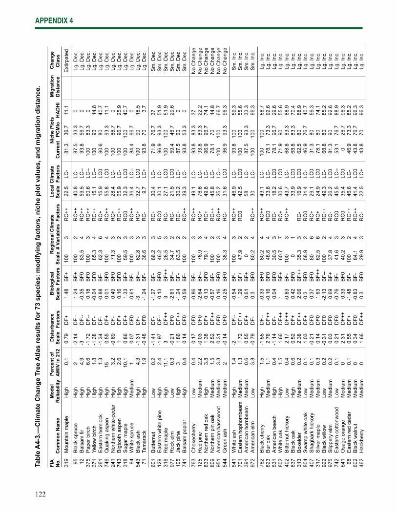
122
APPENDIX 4
319
Mou
ntai
n m
aple
H
igh
0.1
0.79
D
F+
1.48
B
F+
100
3 R
C++
22
.5
LC-
81.3
36
.7
11.1
Ext
irpat
ed
95
Bla
ck s
pruc
e H
igh
2 -2
.14
DF-
- 1.
24
BF+
10
0 2
RC
++
40.8
LC
- 87
.5
33.3
0
Lg
. Dec
. 1
2 B
alsa
m fi
r H
igh
4.9
-3
DF-
- -0
.35
BF0
83
.5
4 R
C++
59
.5
LC--
93
.8
56.7
0
Lg
. Dec
.37
5 P
aper
birc
h H
igh
6.6
-1.7
2 D
F--
0.18
B
F0
100
3 R
C++
60
.6
LC--
10
0 83
.3
0
Lg. D
ec.
371
Yello
w b
irch
Hig
h 1.
8 -1
.38
DF-
-0
.04
BF0
85
.3
4 R
C++
15
.1
LC--
10
0 90
14
.8
Lg
. Dec
.26
1 E
aste
rn h
emlo
ck
Hig
h 1.
3 -1
.34
DF-
-0
.88
BF-
62
.3
6 R
C+
15.9
LC
0 90
.6
80
40.7
Lg. D
ec.
746
Qua
king
asp
en
Hig
h 15
0.
55
DF+
0.
01
BF0
10
0 4
RC
++
55.8
LC
0 10
0 93
.3
11.1
Lg. D
ec.
241
Nor
ther
n w
hite
-ced
ar
Hig
h 3.
2 -0
.69
DF-
0.
49
BF0
71
.3
3 R
C+
28.4
LC
- 10
0 66
.7
0
Lg. D
ec.
743
Big
toot
h as
pen
Hig
h 2.
6 1
DF+
0.
16
BF0
10
0 2
RC
++
65.9
LC
- 10
0 96
.7
25.9
Lg. D
ec.
318
Sug
ar m
aple
H
igh
10.1
0.
86
DF+
1.
33
BF+
59
.5
3 R
C0
32.3
LC
0 10
0 10
0 40
.7
Lg
. Dec
. 9
4 W
hite
spr
uce
Med
ium
1
0.07
D
F0
-0.6
1 B
F-
100
3 R
C++
36
.4
LC--
84
.4
66.7
0
Lg
. Dec
.54
3 B
lack
ash
H
igh
4.3
-1.3
1 D
F-
-3
BF-
- 62
.8
3 R
C+
32.7
LC
0 10
0 90
18
.5
Lg
. Dec
. 7
1 Ta
mar
ack
Hig
h 1.
9 -0
.48
DF0
-1
.24
BF-
36
.6
3 R
C-
9.7
LC+
93.8
70
3.
7
Lg. D
ec.
601
But
tern
ut
Low
0.
2 -1
.41
DF-
-1
.27
BF-
66
.2
3 R
C+
30.4
LC
- 71
.9
76.7
37
Sm
. Dec
.12
9 E
aste
rn w
hite
pin
e H
igh
2.4
-1.9
7 D
F--
0.13
B
F0
46.2
5
RC
0 30
.1
LC-
96.9
93
.3
51.9
Sm
. Dec
.31
6 R
ed m
aple
H
igh
11.1
3
DF+
+ 3
BF+
+ 26
.5
3 R
C-
27.1
LC
0 10
0 10
0 51
.9
S
m. D
ec.
977
Roc
k el
m
Low
0.
3 -0
.21
DF0
-2
.61
BF-
- 34
.7
2 R
C-
21.5
LC
0 59
.4
46.7
29
.6
S
m. D
ec.
105
Jack
pin
e H
igh
3 1.
86
DF+
+ -1
.24
BF-
63
.5
2 R
C+
30.2
LC
+ 87
.5
60
0
Sm
. Dec
.74
1 B
alsa
m p
opla
r H
igh
0.4
0.14
D
F0
-0.5
9 B
F-
100
2 R
C++
39
.3
LC-
93.8
53
.3
0
Sm
. Dec
.
763
Cho
kech
erry
Lo
w
0.4
0.17
D
F0
-0.8
6 B
F-
100
3 R
C++
49
.1
LC-
93.8
83
.3
37
N
o C
hang
e12
5 R
ed p
ine
Med
ium
2.
2 -0
.03
DF0
-2
.64
BF-
- 76
.9
3 R
C+
76.6
LC
- 93
.8
83.3
22
.2
N
o C
hang
e83
3 N
orth
ern
red
oak
Hig
h 3.
8 1.
38
DF+
0.
13
BF0
79
.1
4 R
C+
49.8
LC
- 96
.9
96.7
74
.1
N
o C
hang
e80
9 N
orth
ern
pin
oak
Med
ium
1.
5 2.
52
DF+
+ -0
.57
BF-
10
0 2
RC
++
45.8
LC
- 78
.1
70
14.8
No
Cha
nge
951
Am
eric
an b
assw
ood
Med
ium
3.
3 0.
31
DF0
0.
16
BF0
10
0 3
RC
++
25.2
LC
--
100
100
66.7
No
Cha
nge
544
Gre
en a
sh
Med
ium
2
-0.1
4 D
F0
-0.2
5 B
F0
38.3
4
RC
- 31
.6
LC0
96.9
93
.3
96.3
No
Cha
nge
541
Whi
te a
sh
Hig
h 1.
4 -2
D
F--
-0.5
4 B
F-
100
3 R
C++
46
.9
LC-
93.8
10
0 59
.3
S
m. I
nc.
701
Eas
tern
hop
horn
beam
M
ediu
m
1.3
1.72
D
F++
1.29
B
F+
47.9
2
RC
0 42
.5
LC0
100
100
55.6
Sm
. Inc
.39
1 A
mer
ican
hor
nbea
m
Med
ium
0.
6 0.
55
DF+
0.
61
BF+
0
2
58
LC-
87.5
93
.3
33.3
Sm
. Inc
.97
2 A
mer
ican
elm
Lo
w
3.8
-0.7
9 D
F-
0.3
BF0
80
.2
4 R
C++
30
LC
- 10
0 10
0 96
.3
S
m. I
nc.
762
Bla
ck c
herr
y H
igh
1.5
-1.5
5 D
F--
-0.3
3 B
F0
80.2
4
RC
++
43.1
LC
- 10
0 10
0 66
.7
Lg
. Inc
.82
3 B
ur o
ak
Med
ium
1.
1 2.
76
DF+
+ -0
.16
BF0
48
.6
4 R
C0
33.8
LC
- 78
.1
73.3
92
.6
Lg
. Inc
.53
1 A
mer
ican
bee
ch
Hig
h 0.
4 -1
.14
DF-
0.
04
BF0
30
.5
3 R
C-
18.2
LC
0 78
.1
96.7
29
.6
Lg
. Inc
.80
2 W
hite
oak
H
igh
1.5
1.66
D
F++
1 B
F+
60.7
7
RC
+ 30
.6
LC0
71.9
90
55
.6
Lg
. Inc
.40
2 B
itter
nut h
icko
ry
Low
0.
4 2.
17
DF+
+ -0
.83
BF-
10
0 3
RC
++
43.7
LC
- 68
.8
83.3
88
.9
Lg
. Inc
.83
7 B
lack
oak
H
igh
0.6
0.52
D
F+
0.42
B
F0
0 1
33
.9
LC0
68.8
83
.3
70.4
Lg. I
nc.
313
Box
elde
r M
ediu
m
0.2
2.38
D
F++
2.06
B
F++
35.3
3
RC
- 16
.9
LC0
62.5
80
88
.9
Lg
. Inc
.80
4 S
wam
p w
hite
oak
Lo
w
0.1
1.03
D
F+
-0.3
B
F0
58.9
2
RC
0 31
.4
LC-
46.9
76
.7
40.7
Lg. I
nc.
407
Sha
gbar
k hi
ckor
y M
ediu
m
0.1
-0.2
1 D
F0
0.37
B
F0
80
6 R
C+
29.1
LC
0 31
.3
80
59.3
Lg. I
nc.
317
Silv
er m
aple
M
ediu
m
0.3
0.14
D
F0
1.63
B
F++
62.5
6
RC
+ 24
.9
LC0
78.1
80
74
.1
Lg
. Inc
.92
2 B
lack
will
ow
Low
0.
2 -0
.31
DF0
-2
.13
BF-
- 10
0 2
RC
++
49.3
LC
- 68
.8
80
85.2
Lg. I
nc.
975
Slip
pery
elm
M
ediu
m
0.2
0.03
D
F0
0.69
B
F+
37.8
4
RC
- 26
.2
LC0
81.3
90
92
.6
Lg
. Inc
.74
2 E
aste
rn c
otto
nwoo
d Lo
w
0.1
0.21
D
F0
-0.7
6 B
F-
41.6
3
RC
0 45
.5
LC--
53
.1
76.7
88
.9
Lg
. Inc
.64
1 O
sage
ora
nge
Med
ium
0
2.31
D
F++
0.33
B
F0
40.2
3
RC
0 35
.4
LC0
0 26
.7
96.3
Lg. I
nc.
68
Eas
tern
red
ceda
r M
ediu
m
0.1
0.55
D
F+
-1.4
8 B
F-
100
2 R
C++
46
.6
LC-
46.9
73
.3
85.2
Lg. I
nc.
602
Bla
ck w
alnu
t M
ediu
m
0 0.
34
DF0
-0
.83
BF-
84
.1
4 R
C++
41
.4
LC0
43.8
76
.7
96.3
Lg. I
nc.
462
Hac
kber
ry
Med
ium
0
1.66
D
F++
0.3
BF0
29
.9
3 R
C-
22.5
LC
+ 43
.8
70
96.3
Lg. I
nc.
FIA
Mod
el
Perc
ent o
f D
istu
rban
ce
Bio
logi
cal
Reg
iona
l Clim
ate
Loca
l Clim
ate
Nic
he P
lots
M
igra
tion
Cha
nge
No.
C
omm
on N
ame
Rel
iabi
lity
AWIV
in 2
12
Scal
e Fa
ctor
s Sc
ale
Fact
ors
Scal
e #
Varia
bles
Fac
tors
Sc
ale
Fac
tors
C
urre
nt
PCM
lo
HA
DH
i D
ista
nce
Cla
ss
Tabl
e A
4-3.
—C
limat
e C
hang
e Tr
ee A
tlas
resu
lts fo
r 73
spec
ies:
mod
ifyin
g fa
ctor
s, n
iche
plo
t val
ues,
and
mig
ratio
n di
stan
ce.

123
APPENDIX 4
830
Pin
oak
M
ediu
m
0 -0
.66
DF-
-1
.39
BF-
80
.4
4 R
C++
20
.2
LC-
15.6
46
.7
37
N
ew-B
oth
331
Ohi
o bu
ckey
e Lo
w
0 0.
38
DF0
-1
.92
BF-
- 0
1
56.4
LC
0 3.
1 23
.3
33.3
40
0 km
N
ew-B
oth
373
Riv
er b
irch
Low
0
-0.4
5 D
F0
-0.3
3 B
F0
0 4
39
.4
LC0
28.1
46
.7
33.3
New
-Bot
h90
1 B
lack
locu
st
Low
0
0 D
F0
-0.5
9 B
F-
55.4
3
RC
0 30
.5
LC0
25
66.7
59
.3
N
ew-B
oth
931
Sas
safra
s H
igh
0 0.
48
DF0
-0
.64
BF-
53
.2
4 R
C0
30.5
LC
0 18
.8
60
40.7
20
0 km
N
ew-B
oth
403
Pig
nut h
icko
ry
Hig
h 0
0.21
D
F0
0.4
BF0
33
.9
3 R
C-
13.9
LC
+ 12
.5
73.3
51
.9
200
km
New
-Bot
h68
2 R
ed m
ulbe
rry
Low
0
0.07
D
F0
0.59
B
F+
52.4
4
RC
0 17
.1
LC+
25
66.7
96
.3
100
km
New
-Bot
h49
1 Fl
ower
ing
dogw
ood
Hig
h 0
0.07
D
F0
0.95
B
F+
46.2
7
RC
0 16
.5
LC-
21.9
60
51
.9
200
km
New
-Bot
h55
2 H
oney
locu
st
Low
0
1.9
DF+
+ -0
.54
BF-
32
.4
3 R
C-
30.5
LC
0 9.
4 50
96
.3
200
km
New
-Bot
h62
1 Ye
llow
-pop
lar
Hig
h 0
0.14
D
F0
1.25
B
F+
55.9
6
RC
0 21
.2
LC-
0 23
.3
44.4
20
0 km
N
ew-B
oth
409
Moc
kern
ut h
icko
ry
Hig
h 0
1.69
D
F++
-0.2
8 B
F0
46.7
5
RC
0 20
.6
LC0
12.5
73
.3
55.6
20
0 km
N
ew-B
oth
404
Pec
an
Low
0
-1.2
4 D
F-
-1.7
B
F--
0 2
29
.9
LC-
0 0
14.8
11
00 k
m
New
-Hig
h92
1 P
each
leaf
will
ow
Low
0
0.14
D
F0
-1.6
5 B
F--
999
0
7.9
LC+
28.1
16
.7
14.8
40
0 km
N
ew-H
igh
408
Bla
ck h
icko
ry
Hig
h 0
1.03
D
F+
-2.2
8 B
F--
40.3
3
RC
0 33
.1
LC0
0 0
18.5
60
0 km
N
ew-H
igh
766
Wild
plu
m
Low
0
0.48
D
F0
-1.3
4 B
F-
0 1
33
.2
LC0
34.4
53
.3
18.5
New
-Hig
h45
2 N
orth
ern
cata
lpa
Low
0
0.93
D
F+
-1.5
8 B
F--
0 1
33
.9
LC--
0
16.7
37
11
00 k
m
New
-Hig
h80
6 S
carle
t oak
H
igh
0 -0
.34
DF0
0.
71
BF+
0
3
24.7
LC
+ 6.
3 36
.7
48.1
60
0 km
N
ew-H
igh
731
Syc
amor
e M
ediu
m
0 1.
28
DF+
-0
.9
BF-
68
.2
2 R
C+
33.7
LC
0 0
36.7
85
.2
200
km
New
-Hig
h46
1 S
ugar
berr
y M
ediu
m
0 -0
.17
DF0
0.
64
BF+
0
2
35.9
LC
- 0
0 18
.5
1100
km
N
ew-H
igh
826
Chi
nkap
in o
ak
Med
ium
0
1.17
D
F+
-0.6
6 B
F-
37.1
3
RC
- 43
LC
- 3.
1 33
.3
77.8
40
0 km
N
ew-H
igh
817
Shi
ngle
oak
M
ediu
m
0 1.
31
DF+
-0
.73
BF-
0
2
34.9
LC
+ 0
10
37
400
km
New
-Hig
h47
1 E
aste
rn re
dbud
M
ediu
m
0 0.
9 D
F+
-0.0
4 B
F0
100
3 R
C++
83
.7
LC--
0
3.3
85.2
40
0 km
N
ew-H
igh
835
Pos
t oak
H
igh
0 2.
17
DF+
+ -0
.59
BF-
78
.7
5 R
C+
64.7
LC
- 0
3.3
48.1
60
0 km
N
ew-H
igh
824
Bla
ckja
ck o
ak
Med
ium
0
1.55
D
F++
0.2
BF0
66
.2
3 R
C+
62.1
LC
- 0
0 51
.9
600
km
New
-Hig
h52
1 C
omm
on p
ersi
mm
on
Med
ium
0
1.17
D
F+
0.95
B
F+
100
3 R
C++
31
.9
LC0
0 0
25.9
60
0 km
N
ew-H
igh
693
Bla
ckgu
m
Hig
h 0
1.45
D
F+
0.83
B
F+
39.9
3
RC
- 39
.3
LC-
6.3
30
51.9
40
0 km
N
ew-H
igh
832
Che
stnu
t oak
H
igh
0 1.
38
DF+
1.
29
BF+
17
.4
6 R
C--
36
.2
LC0
15.6
53
.3
48.1
60
0 km
N
ew-H
igh
FIA
Mod
el
Perc
ent o
f D
istu
rban
ce
Bio
logi
cal
Reg
iona
l Clim
ate
Loca
l Clim
ate
Nic
he P
lots
M
igra
tion
Cha
nge
No.
C
omm
on N
ame
Rel
iabi
lity
AWIV
in 2
12
Scal
e Fa
ctor
s Sc
ale
Fact
ors
Scal
e #
Varia
bles
Fac
tors
Sc
ale
Fac
tors
C
urre
nt
PCM
lo
HA
DH
i D
ista
nce
Cla
ss
Tabl
e A
4-3
(con
tinue
d).—
Clim
ate
Cha
nge
Tree
Atla
s re
sults
for 7
3 sp
ecie
s: m
odify
ing
fact
ors,
nic
he p
lot v
alue
s, a
nd m
igra
tion
dist
ance
.

124
APPENDIX 4
Class 1: Extirpated
Only one species, mountain maple, Acer spicatum, fell into this class, and it is very rare now. The metrics of HLE, HLE, MR+, DF+, BF+, RC++, LC- indicate that the model for the species was good and that both low and high emissions scenarios are projected to extirpate the habitat. However, both the disturbance and biological MODFACs show the species could do somewhat better than the models suggest. Conversely, the species is highly connected to climatic variables as regional drivers (growing season temperatures), indicating the species is probably quite sensitive to temperature changes.
Figure A4-4.—(Future : Current) suitable habitat ratios and modifi cation factors for Class 2 (large decline) species, sorted by decreasing disturbance modifi cation scores, such that species with MODFACs > 0 may do better than modeled, while species with MODFACs < 0 may do worse than modeled.
Class 2: Large Decline
This class has 12 species that are currently very common and important in the region, but show large potential declines in suitable habitat (Fig. A4-4). All currently exist in at least 146 of the 225 (65 percent) 20 x 20 km pixels in Wisconsin 212; and all but one species, white spruce, have high model reliability scores.
Black spruce—Black spruce, Picea mariana, has the most serious projected decline in suitable habitat, reduced to 10 percent of current for the average of low emissions scenarios and 8 percent for the average
125
APPENDIX 4
high emissions scenarios. The niche plot (Fig. A4-3) clearly shows no current black spruce occupation in any of the HadHi niche and only a third of the PCMLo niche. Black spruce also appears to be highly sensitive to the disturbance factors (DF--) that would increase in a warmed climate, especially drought, insect pests, and fi re topkill. That, coupled with high regional sensitivity to temperature variables (RC++), indicates the species may do worse than indicated by the niche modeling. Although somewhat benefi ted by biological factors (BF+), especially shade tolerance, this species may be the most at risk among all (besides mountain maple) in the region.
Balsam fi r—Balsam fi r, Abies balsamea, has traits similar to black spruce as far as sensitivity to climate change, but our assessment shows it may be slightly more resilient. It is found in the same habitats and in the same parts of Wisconsin 212, and the niche modeling shows a reduction of suitable habitat to 13 percent of current for the average low emissions scenarios and 9 percent for the high emissions scenarios. Area of habitat is not projected to be reduced as much, however. For example, the number of cells projected to remain with habitat is almost twice (79 versus 41 out of 225 cells) for the fi r over the spruce under the HadHi emissions scenario. The other scores of DF--, BF0, RC++, and LC-- again show the extra sensitivity to disturbance factors (especially insect pests, drought, and fi re topkill) and regional climate factors (growing season and July temperatures), again indicating that the species may do worse than the models project. The niche plot clearly shows that the species does not now exist in any location under temperatures projected under HadHi.
Northern white-cedar—Northern white-cedar, Thuja occidentalis, is projected have its suitable habitat reduced to 30 percent of current for average low emissions and 23 percent for high emissions. The niche plot shows no current occupancy in the future HadHi temperature and precipitation regimes, and about two-thirds occupancy in the PCMLo niche. The
other metrics, DF-, BF0, RC+, LC-, indicate no serious issues relative to the other factors not considered in the niche models, indicating relatively high confi dence.
Yellow birch—Yellow birch, Betula alleghaniensis, is projected to have its suitable habitat reduced to 29 percent of current for the low emissions scenarios and 16 percent for the high emissions scenarios. The biological factors on the whole are neutral (BF0) but the high dispersal ability may be a benefi t under climate change, given that the climate niche within the region is at the periphery of the species tolerance zone. The other factors (DF-, RC++, LC--), like those from the habitat model (HL--, HH--), suggest further potential restrictions for this species under climate change, and that it may not do even as well as projected. The species model indicates a strong climate infl uence at the regional scale (RC++) and that climate is less of a driver at local scales (LC--). In addition, a more negative trend in response to disturbance (DF-) is infl uenced by sensitivity to fi re topkill and insect pests.
Paper birch—Paper birch, Betula papyrifera, is the fourth highest species in terms of current modeled importance value, and Wisconsin 212 accounts for 6.6 percent of the total summed importance value for the species across the entire eastern United States. It is projected to have its suitable habitat substantially reduced to 38 percent of current for the average low emissions scenarios and 12 percent for the high emissions scenarios. This projected loss may be exacerbated by negative response to drought and fi re topkill, thus infl uencing the negative disturbance score (DF--). The other metrics do not strongly suggest further climate change stress to the species, with BF0 and LC--; and while RC++ on the surface would raise concerns, the model is primarily driven by the local scale variables.
Quaking aspen—Quaking aspen, Populus tremuloides, has the highest current modeled importance value and occupies all 225 cells in Wisconsin 212. The suitable habitat is projected
126
APPENDIX 4
to change little in terms of the number of cells (minimum of 218 cells), but the quality of the habitat is projected to decline to 44 percent of current for low the emissions scenarios and 16 percent for the high emissions scenarios. The strong regional climate infl uence (RF++, to a lesser extent local, LC0) and shift in climatic niche space points further to a pattern of reduced habitat quality but not occupancy within the region. The species characteristics and these metrics suggest that the species may be able to do better under climate change than the habitat model projects, with a more positive response to disturbance (DF+) because of its broad temperature tolerances (after all it is found throughout Canada and much of the western United States), and balancing by biological factors (BF0).
White spruce—White spruce, Picea glauca, is projected to decline in suitable habitat to 54 percent of current for low emissions scenarios and 39 percent for the low emissions scenarios. The species model is driven by a strong regional climate infl uence (RC++), with little local climate infl uence (LC--). Under the highest emissions scenario, HadHi, the temperature and precipitation niche would have no contemporary habitat for the species, further highlighting the species potential risk to climate change impacts. The species is less sensitive to disturbance factors (DF0), but has a more negative biological profi le (BF-). It is important to reiterate the lower model reliability (MR0) for this species when interpreting the species results, but the overall negative metrics provide good evidence of likely negative habitat response to climate change.
Eastern hemlock—Eastern hemlock, Tsuga canadensis, projected suitable habitat declines to 17 percent of current under the high emissions scenarios and to 42 percent of current under the low emissions scenarios. This species is moderately climate driven at regional scales (RC+, LC0) with temperature serving as the primary determinant. Perhaps most signifi cant to persistence over the next century is its sensitivity to disturbance and biological factors (DF-, BF-). The major negative factor now is
its susceptibility to hemlock wooly adelgid, and this, combined with negative response to drought, will likely push losses beyond those projected. Eastern hemlock is not a valuable timber species, but it has signifi cant ecological and aesthetic value. Eastern hemlocks often grow in the lower, wetter areas along streams, and thus provide cooler habitats for many other organisms.
Sugar maple—Sugar maple, Acer saccharum, has the third highest weighted importance value (suitable habitat) and is found throughout Wisconsin 212. It also accounts for just over 10 percent of the total summed importance values across the eastern United States, so it is an extremely important species. While the species is projected to decline in suitable habitat to 57 percent of current under the average low emissions scenarios and 32 percent under the high emissions scenarios, the species is projected to continue to exist in all 225 cells for all models. The species model utilized a variety of predictors and is not highly driven by climate factors alone at both regional and local scales (RC0, LC0). The other metrics suggest many characteristics that may benefi t the species under climate change (DF+, BF+), most notably its positive score related to its light competition and its few disease and insect predators. Thus, the species may do better than projected in our suitable habitat models. However, the niche plot shows that the species does not now exist in temperature/precipitation regimes that would occur for nearly 60 percent of the region under the most severe model tested (HadHi).
Black ash—Black ash, Fraxinus nigra, despite little projected change in occupancy within the region (from 225 cells to a minimum of 215 cells), the weighted importance value is projected to decline to 68 percent of its current habitat for the emissions scenario and 51 percent for the high emissions scenario. Like many species in this class, the climatic niche overlap within the region shows a shift out of much of the species range under the highest emissions scenario (HadHi), which is also corroborated by a regional climate

127
APPENDIX 4
infl uence (RC+, LC0). The species’ susceptibility to emerald ash borer, of course, is a major limitation to its persistence and is refl ected in a negative disturbance score (DF-). In addition, the strong negative biological factor score (BF--), resulting in part from limited dispersal and seedling establishment, puts this species at a much greater risk in the future than the climate change habitat models alone would suggest.
Tamarack—Tamarack, Larix laricina, is projected to remain a part of Wisconsin 212 with little change in the extent, but with declines in suitable habitat to 71 percent of current for the low emissions scenarios and 53 percent for the high emissions scenarios. Unlike the other species in this class, it shows more local climate drivers (LC+, RC-) and the species model is most infl uenced by soil variables. This lack of regional sensitivity to climate likely accounts for the stability of occupancy despite the fact that the climatic niche moves substantially above its present temperature zone under HadHi. The other metrics do not strongly indicate greater risk under climate change (DF0, BF-), but the species negative competitive score for light may restrict establishment into new areas.
Bigtooth aspen—Bigtooth aspen, Populus. grandidentata, has a projected suitable habitat response that greatly depends on the emissions scenarios. Under average low emissions, a modest decline to 69 percent of current habitat is projected, compared to 26 percent under the high emissions scenario. These changes are brought about by a greater shift northward, thus loss of occupancy, with higher emissions (from 223 cells to a minimum of 142 cells under HadHi). This pattern is refl ected by a strong regional climate infl uence (RC++, LC-), with the regional climate niche maps indicating that the cooler-wetter areas are the habitats most likely to remain in suitable habitat. The species has a positive disturbance profi le (DF+) resulting in part from relatively lower susceptibility to insect pests. The biological factors do not indicate further susceptibility (BC0), and the total weight of evidence suggests that the habitat models likely provide a good place to begin considering the potential changes for this species within the region.
A forested landscape in northern Wisconsin.
Pho
to b
y To
m M
atth
iae,
Che
quam
egon
-Nic
olet
Nat
iona
l For
est

128
APPENDIX 4
Class 3: Small Decline
This group consists of six species that vary greatly in current importance, in quality of models, and in variation in response between emissions scenarios (Fig. A4-5). In general, the species show little or no change at the low emission level, but under high emissions, the habitat is reduced. The exception is Balsam poplar (Populus balsamifera), which shows a reduction under the low emissions scenerio but no change under the high emissions scenario. We discuss three of the six species here (all three with highly reliable models).
Jack pine—Jack pine, Pinus banksiana, models show some expansion of potentially occupied cells, though it is not certain all these new cells can edaphically support jack pine. However, the overall suitable habitat is reduced to 84 percent of current for the low emissions scenarios and 62 percent for the high emissions scenarios. The temperature/precipitation niche plot clearly shows that under low emissions, the temperatures and precipitation can host the species but not so for high emission outcomes. The metrics of DF++, BF-, RC+, LC+ could indicate that the species
Figure A4-5.—(Future : Current) suitable habitat ratios and modifi cation factors for Class 3 (small decline) species, sorted by decreasing disturbance modifi cation scores, such that species with MODFACs > 0 may do better than modeled, while species with MODFACs < 0 may do worse than modeled.
will do better under the predicted disturbance regimes; and it is not particularly controlled by temperature variables (growing season precipitation is the only important climate variable, and that at the local scale) and thus may do just fi ne in a slightly, but not extremely, warmed climate.
Red maple—Red maple, Acer rubrum, is one of the most adaptable species on the planet and is expanding greatly in the eastern United States. Consequently, we have always been uneasy with estimates of reduced suitable habitat according to our models; for Wisconsin 212, we model suitable habitat reductions to 81 (low emissions) and 57 percent (high emissions) of current size even though we model no loss in pixels with habitat. However, when we added the MODFAC information, we see the maximum advantages, compared to all 134 species, for both disturbance (DF++) and biological (BF++) factors. So this species will likely do much better than modeled. In fact, based on other evidence, the species may continue to fl ourish regardless of the climate changes underway. Abrams (1998) describes red maple as a “supergeneralist” that has been expanding greatly throughout much of the eastern United States in recent decades and thrives
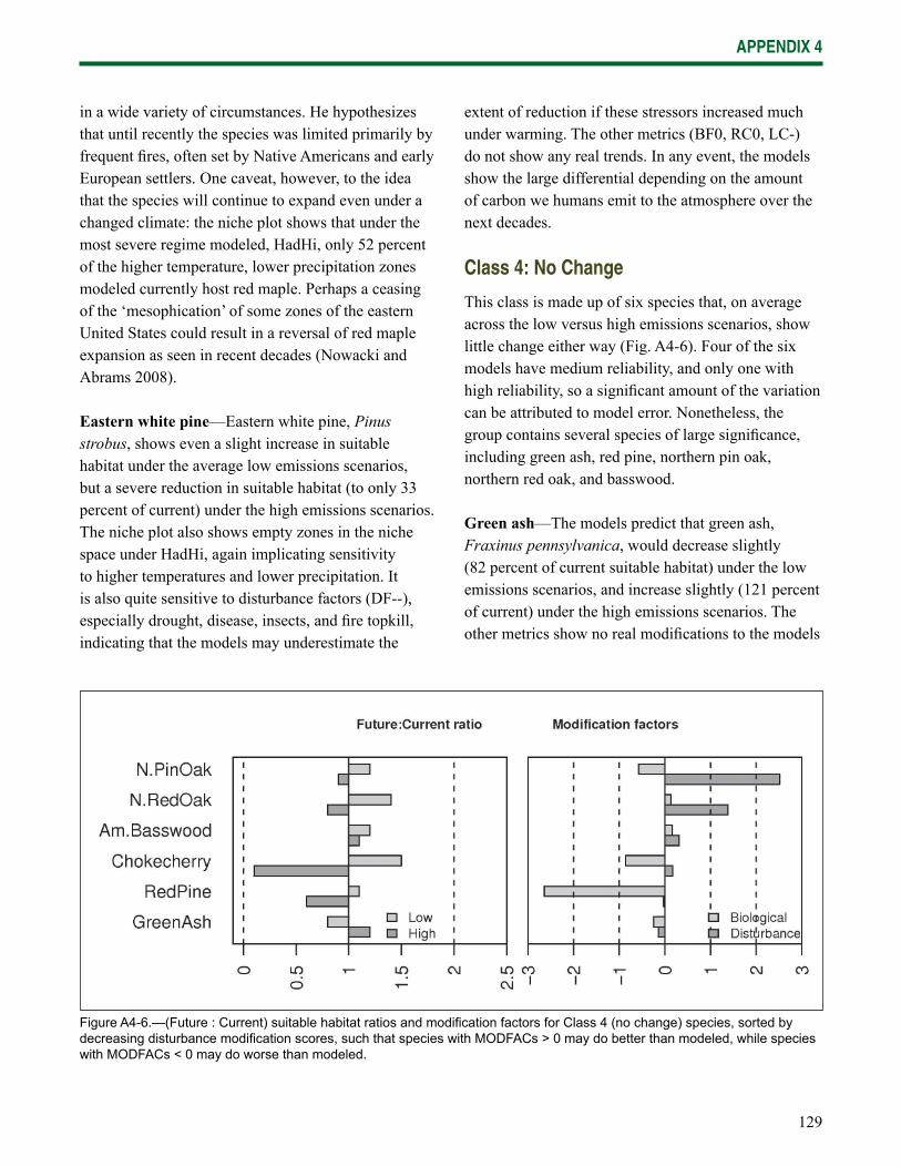
129
APPENDIX 4
in a wide variety of circumstances. He hypothesizes that until recently the species was limited primarily by frequent fi res, often set by Native Americans and early European settlers. One caveat, however, to the idea that the species will continue to expand even under a changed climate: the niche plot shows that under the most severe regime modeled, HadHi, only 52 percent of the higher temperature, lower precipitation zones modeled currently host red maple. Perhaps a ceasing of the ‘mesophication’ of some zones of the eastern United States could result in a reversal of red maple expansion as seen in recent decades (Nowacki and Abrams 2008).
Eastern white pine—Eastern white pine, Pinus strobus, shows even a slight increase in suitable habitat under the average low emissions scenarios, but a severe reduction in suitable habitat (to only 33 percent of current) under the high emissions scenarios. The niche plot also shows empty zones in the niche space under HadHi, again implicating sensitivity to higher temperatures and lower precipitation. It is also quite sensitive to disturbance factors (DF--), especially drought, disease, insects, and fi re topkill, indicating that the models may underestimate the
Figure A4-6.—(Future : Current) suitable habitat ratios and modifi cation factors for Class 4 (no change) species, sorted by decreasing disturbance modifi cation scores, such that species with MODFACs > 0 may do better than modeled, while species with MODFACs < 0 may do worse than modeled.
extent of reduction if these stressors increased much under warming. The other metrics (BF0, RC0, LC-) do not show any real trends. In any event, the models show the large differential depending on the amount of carbon we humans emit to the atmosphere over the next decades.
Class 4: No Change
This class is made up of six species that, on average across the low versus high emissions scenarios, show little change either way (Fig. A4-6). Four of the six models have medium reliability, and only one with high reliability, so a signifi cant amount of the variation can be attributed to model error. Nonetheless, the group contains several species of large signifi cance, including green ash, red pine, northern pin oak, northern red oak, and basswood.
Green ash—The models predict that green ash, Fraxinus pennsylvanica, would decrease slightly (82 percent of current suitable habitat) under the low emissions scenarios, and increase slightly (121 percent of current) under the high emissions scenarios. The other metrics show no real modifi cations to the models
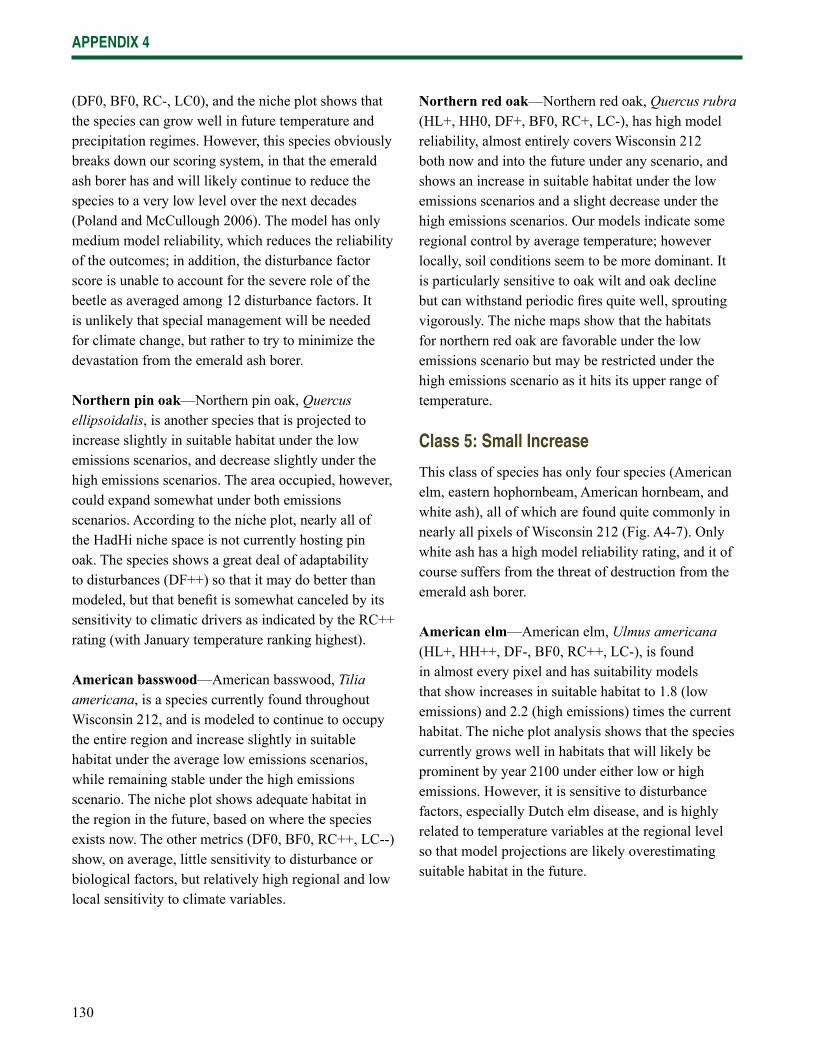
130
APPENDIX 4
(DF0, BF0, RC-, LC0), and the niche plot shows that the species can grow well in future temperature and precipitation regimes. However, this species obviously breaks down our scoring system, in that the emerald ash borer has and will likely continue to reduce the species to a very low level over the next decades (Poland and McCullough 2006). The model has only medium model reliability, which reduces the reliability of the outcomes; in addition, the disturbance factor score is unable to account for the severe role of the beetle as averaged among 12 disturbance factors. It is unlikely that special management will be needed for climate change, but rather to try to minimize the devastation from the emerald ash borer.
Northern pin oak—Northern pin oak, Quercus ellipsoidalis, is another species that is projected to increase slightly in suitable habitat under the low emissions scenarios, and decrease slightly under the high emissions scenarios. The area occupied, however, could expand somewhat under both emissions scenarios. According to the niche plot, nearly all of the HadHi niche space is not currently hosting pin oak. The species shows a great deal of adaptability to disturbances (DF++) so that it may do better than modeled, but that benefi t is somewhat canceled by its sensitivity to climatic drivers as indicated by the RC++ rating (with January temperature ranking highest).
American basswood—American basswood, Tilia americana, is a species currently found throughout Wisconsin 212, and is modeled to continue to occupy the entire region and increase slightly in suitable habitat under the average low emissions scenarios, while remaining stable under the high emissions scenario. The niche plot shows adequate habitat in the region in the future, based on where the species exists now. The other metrics (DF0, BF0, RC++, LC--) show, on average, little sensitivity to disturbance or biological factors, but relatively high regional and low local sensitivity to climate variables.
Northern red oak—Northern red oak, Quercus rubra (HL+, HH0, DF+, BF0, RC+, LC-), has high model reliability, almost entirely covers Wisconsin 212 both now and into the future under any scenario, and shows an increase in suitable habitat under the low emissions scenarios and a slight decrease under the high emissions scenarios. Our models indicate some regional control by average temperature; however locally, soil conditions seem to be more dominant. It is particularly sensitive to oak wilt and oak decline but can withstand periodic fi res quite well, sprouting vigorously. The niche maps show that the habitats for northern red oak are favorable under the low emissions scenario but may be restricted under the high emissions scenario as it hits its upper range of temperature.
Class 5: Small Increase
This class of species has only four species (American elm, eastern hophornbeam, American hornbeam, and white ash), all of which are found quite commonly in nearly all pixels of Wisconsin 212 (Fig. A4-7). Only white ash has a high model reliability rating, and it of course suffers from the threat of destruction from the emerald ash borer.
American elm—American elm, Ulmus americana (HL+, HH++, DF-, BF0, RC++, LC-), is found in almost every pixel and has suitability models that show increases in suitable habitat to 1.8 (low emissions) and 2.2 (high emissions) times the current habitat. The niche plot analysis shows that the species currently grows well in habitats that will likely be prominent by year 2100 under either low or high emissions. However, it is sensitive to disturbance factors, especially Dutch elm disease, and is highly related to temperature variables at the regional level so that model projections are likely overestimating suitable habitat in the future.
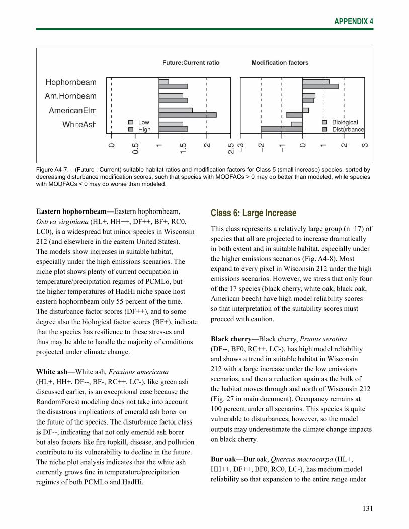
131
APPENDIX 4
Eastern hophornbeam—Eastern hophornbeam, Ostrya virginiana (HL+, HH++, DF++, BF+, RC0, LC0), is a widespread but minor species in Wisconsin 212 (and elsewhere in the eastern United States). The models show increases in suitable habitat, especially under the high emissions scenarios. The niche plot shows plenty of current occupation in temperature/precipitation regimes of PCMLo, but the higher temperatures of HadHi niche space host eastern hophornbeam only 55 percent of the time. The disturbance factor scores (DF++), and to some degree also the biological factor scores (BF+), indicate that the species has resilience to these stresses and thus may be able to handle the majority of conditions projected under climate change.
White ash—White ash, Fraxinus americana (HL+, HH+, DF--, BF-, RC++, LC-), like green ash discussed earlier, is an exceptional case because the RandomForest modeling does not take into account the disastrous implications of emerald ash borer on the future of the species. The disturbance factor class is DF--, indicating that not only emerald ash borer but also factors like fi re topkill, disease, and pollution contribute to its vulnerability to decline in the future. The niche plot analysis indicates that the white ash currently grows fi ne in temperature/precipitation regimes of both PCMLo and HadHi.
Class 6: Large Increase
This class represents a relatively large group (n=17) of species that all are projected to increase dramatically in both extent and in suitable habitat, especially under the higher emissions scenarios (Fig. A4-8). Most expand to every pixel in Wisconsin 212 under the high emissions scenarios. However, we stress that only four of the 17 species (black cherry, white oak, black oak, American beech) have high model reliability scores so that interpretation of the suitability scores must proceed with caution.
Black cherry—Black cherry, Prunus serotina (DF--, BF0, RC++, LC-), has high model reliability and shows a trend in suitable habitat in Wisconsin 212 with a large increase under the low emissions scenarios, and then a reduction again as the bulk of the habitat moves through and north of Wisconsin 212 (Fig. 27 in main document). Occupancy remains at 100 percent under all scenarios. This species is quite vulnerable to disturbances, however, so the model outputs may underestimate the climate change impacts on black cherry.
Bur oak—Bur oak, Quercus macrocarpa (HL+, HH++, DF++, BF0, RC0, LC-), has medium model reliability so that expansion to the entire range under
Figure A4-7.—(Future : Current) suitable habitat ratios and modifi cation factors for Class 5 (small increase) species, sorted by decreasing disturbance modifi cation scores, such that species with MODFACs > 0 may do better than modeled, while species with MODFACs < 0 may do worse than modeled.
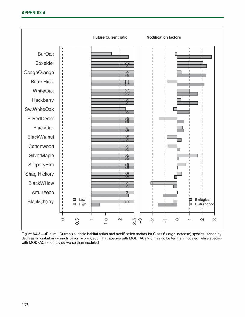
132
APPENDIX 4
Figure A4-8.—(Future : Current) suitable habitat ratios and modifi cation factors for Class 6 (large increase) species, sorted by decreasing disturbance modifi cation scores, such that species with MODFACs > 0 may do better than modeled, while species with MODFACs < 0 may do worse than modeled.
133
APPENDIX 4
high emissions scenario should be viewed with moderate confi dence. This species shows an expansion of suitable habitat of 1.8 times with the low emissions scenarios and 2.2 times with the high emissions scenarios. The model also indicates that bur oak is not very climatically sensitive, at the regional or local scales. Bur oaks are quite resistant to disturbance factors, being one of the most drought tolerant of oaks. It is favored by periodic fi res that may increase under warming and drought conditions. It is only moderately affected by diseases. The niche map for bur oak shows that under both emissions scenarios, the species currently grows in temperature/precipitation habitats projected for Wisconsin 212.
Black oak—Black oak, Quercus velutina (HL++, HH++, DF+, BF0, LC0), has high model reliability lending confi dence to predictions of the expansion to the entire range, and the large increase in suitable habitat under both the low (4-fold increase) and high (6-fold increase) emissions scenarios (Fig. 27 in main document). It is not much of a climatically driven species regionally (the regional statistic RC could not be calculated) or locally (LC0). Black oak is not very drought tolerant compared to other oaks and is more susceptible to fi re topkill. It is moderately affected by diseases as it can succumb to successive defoliations by gypsy moth. The niche map shows that black oaks would likely handle higher future temperatures (low and high emissions scenarios) with even potentially increased habitat abundance.
White oak—White oak, Quercus alba (HL++, HH++, DF++, BF+, RC+, LC0), also has high model reliability. It shows expansion to the entire Wisconsin 212 and increases in suitable habitat by over 2.8 times for both the low and high emissions scenarios. We expect it to be somewhat climatically driven regionally and less so locally, mainly by growing season and July temperature variables. Since white oak is a generalist and well distributed throughout its entire range,
disturbance and biological factors should not affect it much, although it is quite susceptible to gypsy moth and several diseases. The niche map analysis shows white oaks currently fl ourishing at the higher future temperatures (both emissions scenarios), but under the high emissions scenario, Wisconsin 212 may become too dry in some locations.
Swamp white oak—Swamp white oak, Quercus bicolor (HL++, HH++, DF+, BF0, RC0, LC-), has low model reliability; hence the range expansion and 2-fold (low emissions) to 7-fold (high emissions) increase in suitable habitat predicted by our models should be viewed cautiously. Although it is not a particularly a climate driven species, January temperatures infl uence the regional habitat, and growing season precipitation infl uences the local habitat. It is moderately resistant to fi re. Like most oaks, it is tolerant of a wide range of conditions. The niche map for swamp white oak shows little current growth in the temperature/precipitation regimes of the HadHi scenario; this could indicate some potential restrictions to migration should those conditions be realized. But again, the model is of poor reliability.
Shagbark hickory—Shagbark hickory, Carya ovata (DF0, BF0, RC+, LC0), has medium model reliability and expands to the entire range under the high emissions scenarios and almost so under the low emissions scenarios, and over an 8-fold increase in suitable habitat under both scenarios. Both precipitation and temperature affect the distribution regionally although less so locally. The niche diagram shows habitats increasing under both low and high emissions, although the high emissions scenario can stretch its temperature limit. Shagbark hickory can tolerate a wide range of conditions although it grows best under humid conditions. It does not tolerate fi re very well and is susceptible to many diseases and pests. Overall, MODFACs are generally not signifi cant for this species.
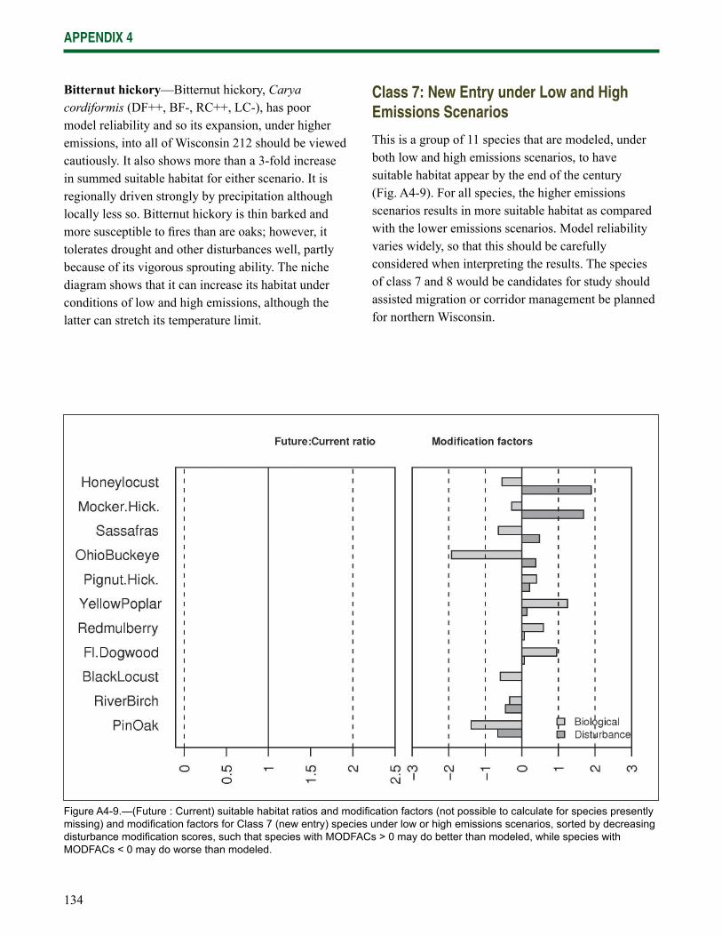
134
APPENDIX 4
Bitternut hickory—Bitternut hickory, Carya cordiformis (DF++, BF-, RC++, LC-), has poor model reliability and so its expansion, under higher emissions, into all of Wisconsin 212 should be viewed cautiously. It also shows more than a 3-fold increase in summed suitable habitat for either scenario. It is regionally driven strongly by precipitation although locally less so. Bitternut hickory is thin barked and more susceptible to fi res than are oaks; however, it tolerates drought and other disturbances well, partly because of its vigorous sprouting ability. The niche diagram shows that it can increase its habitat under conditions of low and high emissions, although the latter can stretch its temperature limit.
Figure A4-9.—(Future : Current) suitable habitat ratios and modifi cation factors (not possible to calculate for species presently missing) and modifi cation factors for Class 7 (new entry) species under low or high emissions scenarios, sorted by decreasing disturbance modifi cation scores, such that species with MODFACs > 0 may do better than modeled, while species with MODFACs < 0 may do worse than modeled.
Class 7: New Entry under Low and High Emissions Scenarios
This is a group of 11 species that are modeled, under both low and high emissions scenarios, to have suitable habitat appear by the end of the century (Fig. A4-9). For all species, the higher emissions scenarios results in more suitable habitat as compared with the lower emissions scenarios. Model reliability varies widely, so that this should be carefully considered when interpreting the results. The species of class 7 and 8 would be candidates for study should assisted migration or corridor management be planned for northern Wisconsin.

135
APPENDIX 4
Pignut hickory—Pignut hickory, Carya glabra (DF0, BF0, RC-, LC+, MD200), shows that suitable habitat for this species could migrate into and substantially cover Wisconsin 212 by the end of the century, especially under the high emissions scenario. Model reliability is high. The niche map analysis clearly show that the species now exists in the temperature/precipitation regimes projected for both emissions scenarios, but especially the low emissions scenario. None of the MODFACs show particularly substantial issues on the models either positively or negatively so that planning can begin with the suitable habitats as mapped. The estimate of MD200 indicates that migration distance needed for the current range boundary to approach the boundary of Wisconsin 212 is less than 200 km; we calculate it to be about 160 km.
Mockernut hickory—Mockernut hickory, Carya tomentosa (DF++, BF0, RC0, LC0, MD200), shows potential expansion into Wisconsin 212 in a manner very similar to pignut hickory. Under the average high emissions scenarios, it would have suitable habitat in about 150 of the 225 cells, and the summed suitable habitat for either mockernut or pignut would approximate that of the resident white spruce or boxelder. Under low emissions, mockernut habitat would be very rare. Because the species shows very positive response to disturbance factors (DF++)—particularly drought, wind, and disease—and is not particularly disadvantaged by other factors, it may do better than modeled. The estimated distance needed to migrate to reach Wisconsin 212 is about 170 km.
Flowering dogwood—Flowering dogwood, Cornus fl orida (DF0, BF+, RC0, LC-, MD200), is another species that is modeled to mirror the hickories in area and habitat quality—a substantial expansion in occupancy from nothing to 70 percent of the region under the high emissions scenario, but only to about 15 percent under the low emissions scenario. The modifying factors for the species are not substantial
in either a positive or negative direction, the model reliability is good, and the niche map shows a reasonable amount of temperature and precipitation habitat in future compared to current occupancy outside the Wisconsin 212 region. Our estimates suggest the species would have to migrate about 180 km to reach the border of Wisconsin 212.
Yellow-poplar—Yellow-poplar, Liriodendron tulipifera (DF0, BF+, RC0, LC-, MD200), is a species of high model reliability showing some migration of low-level suitable habitat into Wisconsin 212, especially under the high emissions scenarios, to an occupancy of about 40 percent of the region (Fig. 28 in main document). The MODFACs are generally moderate, indicating no serious modifi cations to the mapped models may be necessary. We estimate roughly a migration of 200 km to reach the border of Wisconsin 212.
Red mulberry—Red mulberry, Morus rubra (DF0, BF+, RC0, LC+, MD100), shows an increasing trend in habitat with warmer scenarios (Fig. 28 in main document). Though the model reliability is poor, the niche models and the habitat models agree that the warmer scenarios tend to push the habitat northward into Wisconsin 212. However, the habitat did not need to move far, as it currently bounds the southern edge of the region. MODFACs indicate it may do slightly better than modeled.
Sassafras—Sassafras, Sassafras albidum (DF0, BF-, RC0, LC0, MD200), behaves like the other species narrated for this class – this time the occupancy could get up to almost 80 percent of the region under the high emissions scenarios, and about 30 percent under the low scenarios. Again, the model reliability is high and the MODFACs do not register a high level of modifi cation is needed to the modeled outputs. We estimate the species needs to travel only 120 km to reach the border of Wisconsin 212.
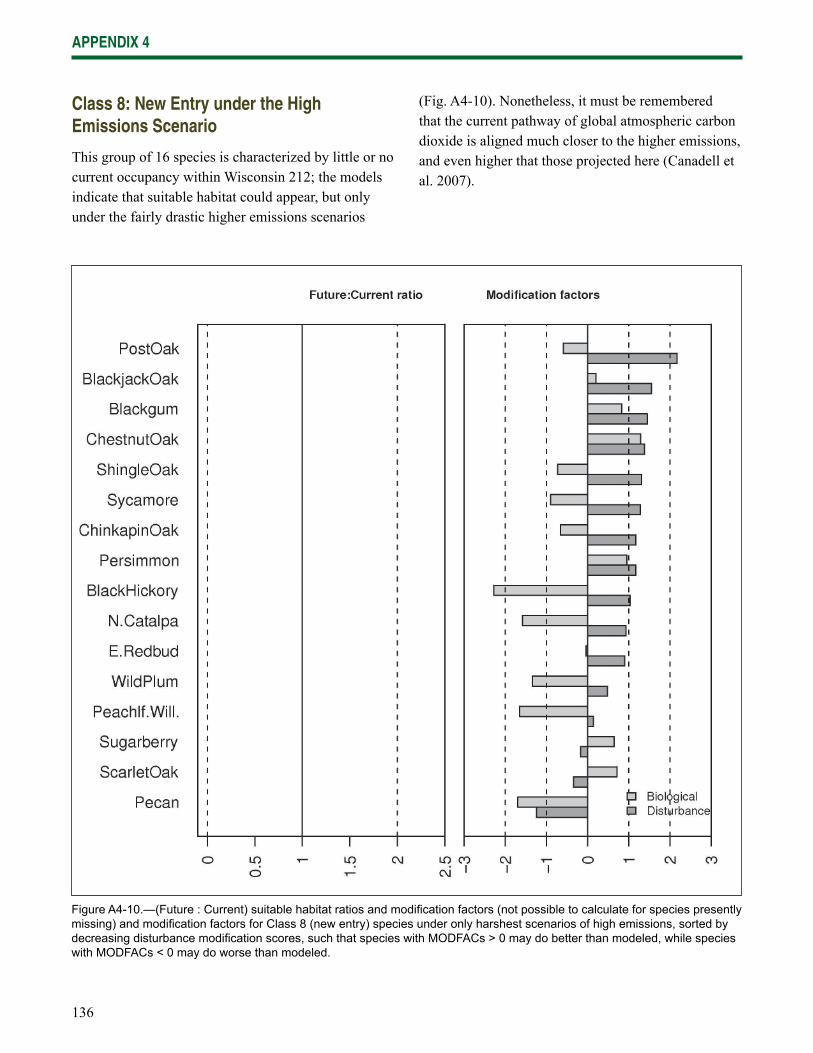
136
APPENDIX 4
Class 8: New Entry under the High Emissions Scenario
This group of 16 species is characterized by little or no current occupancy within Wisconsin 212; the models indicate that suitable habitat could appear, but only under the fairly drastic higher emissions scenarios
Figure A4-10.—(Future : Current) suitable habitat ratios and modifi cation factors (not possible to calculate for species presently missing) and modifi cation factors for Class 8 (new entry) species under only harshest scenarios of high emissions, sorted by decreasing disturbance modifi cation scores, such that species with MODFACs > 0 may do better than modeled, while species with MODFACs < 0 may do worse than modeled.
(Fig. A4-10). Nonetheless, it must be remembered that the current pathway of global atmospheric carbon dioxide is aligned much closer to the higher emissions, and even higher that those projected here (Canadell et al. 2007).
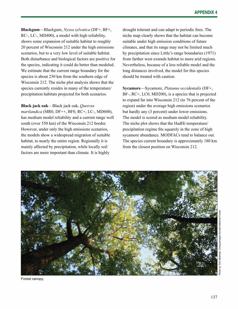
137
APPENDIX 4
Blackgum—Blackgum, Nyssa sylvatica (DF+, BF+, RC-, LC-, MD400), a model with high reliability, shows some expansion of suitable habitat to roughly 20 percent of Wisconsin 212 under the high emissions scenarios, but to a very low level of suitable habitat. Both disturbance and biological factors are positive for the species, indicating it could do better than modeled. We estimate that the current range boundary for the species is about 230 km from the southern edge of Wisconsin 212. The niche plot analysis shows that the species currently resides in many of the temperature/precipitation habitats projected for both scenarios.
Black jack oak—Black jack oak, Quercus marilandica (MR0, DF++, BF0, RC+, LC-, MD600), has medium model reliability and a current range well south (over 550 km) of the Wisconsin 212 border. However, under only the high emissions scenarios, the models show a widespread migration of suitable habitat, to nearly the entire region. Regionally it is mainly affected by precipitation, while locally soil factors are more important than climate. It is highly
drought tolerant and can adapt to periodic fi res. The niche map clearly shows that the habitat can become suitable under high emission conditions of future climates, and that its range may not be limited much by precipitation since Little’s range boundaries (1971) from farther west extends habitat to more arid regions. Nevertheless, because of a less reliable model and the long distances involved, the model for this species should be treated with caution.
Sycamore—Sycamore, Platanus occidentalis (DF+, BF-, RC+, LC0, MD200), is a species that is projected to expand far into Wisconsin 212 (to 76 percent of the region) under the average high emissions scenarios but hardly any (3 percent) under lower emissions. The model is scored as medium model reliability. The niche plot shows that the HadHi temperature/precipitation regime fi ts squarely in the zone of high sycamore abundance. MODFACs tend to balance out. The species current boundary is approximately 180 km from the closest position on Wisconsin 212.
Forest canopy.
Pho
to b
y To
m M
atth
iae,
Che
quam
egon
-Nic
olet
Nat
iona
l For
est
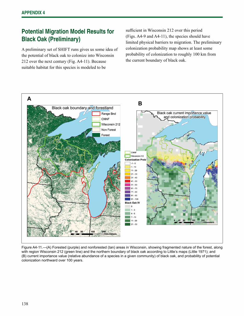
138
APPENDIX 4
Potential Migration Model Results for Black Oak (Preliminary)
A preliminary set of SHIFT runs gives us some idea of the potential of black oak to colonize into Wisconsin 212 over the next century (Fig. A4-11). Because suitable habitat for this species is modeled to be
suffi cient in Wisconsin 212 over this period (Figs. A4-9 and A4-11), the species should have limited physical barriers to migration. The preliminary colonization probability map shows at least some probability of colonization to roughly 100 km from the current boundary of black oak.
Figure A4-11.—(A) Forested (purple) and nonforested (tan) areas in Wisconsin, showing fragmented nature of the forest, along with region Wisconsin 212 (green line) and the northern boundary of black oak according to Little’s maps (Little 1971); and (B) current importance value (relative abundance of a species in a given community) of black oak, and probability of potential colonization northward over 100 years.
AB
139
APPENDIX 4
Summary
Our evaluations suggest that 73 of 134 tree species need to be considered with respect to potential impacts of climate change. Of these 73, we see the entire range of possibilities, from extirpation to long distance migration, as represented by our eight classes of species. For the fi rst time, we have included many sources of ancillary information from literature surveys to inform the calculation of modifying factor scores, dissection of the individual RandomForest models to assess regional and local variable importances, and estimates of distances from the current occupied polygons to the closest edge of Wisconsin 212. We also rely on the ‘model reliability’ rating to give some indication of confi dence in the model outputs.
The work of Woodall et al. (2009) has helped lend confi dence in the overall validity of these models. They studied seedling numbers versus biomass of larger trees for 40 species that we also have modeled, for many thousands of FIA points throughout the eastern United States. They plotted both seedling numbers and tree biomass against latitude to show whether there is a difference in optimal or peak latitude between the two measures. They found a tendency for northward migration for a number of them; and for 37 of the 40 species, their results were congruent with our models.
There are still many assumptions and qualifi ers associated with this work. Some of them are unique to empirical statistical models, but most are common to any modeling that requires estimation into an unknown future. We however attempt to overcome some traditional limitations associated with statistical models by using FIA abundance data with a tri-model approach using the latest decision-tree based, data-mining approach that uncovers the nonlinear, high-dimensional nature of the data which gives more accurate predictions. With the addition of the MODFACs and other attributes, we attempt to allow at
least a qualitative modifi cation of the RandomForest outputs to account for factors that cannot be appropriately modeled. This twin approach begins to address the problems and uncertainties associated with on-the-ground decisionmaking, leading to better management.
Our group aims to continue this work in evaluating potential migration under various scenarios, land use confi gurations, and with other species
Literature Cited
Allen, C.; Macaladyb, A.; Chenchounic, H.; Bachelet, D.; McDowell, N.; Vennetier, M.; Kitzberger, T.; Rigling, A.; Breshear, D.; Hoggi, E.; Gonzalezk, P.; Fensham, R.; Zhangm, Z.; Castron, J.; Demidavao, N.; Lim, J.-H.; Allard, G.; Running, S.; Semerci, A.; Cobb, N. 2010. A global overview of drought and heat-induced tree mortality reveals emerging climate change risks for forests. Forest Ecology and Management. 259: 660-684.
Canadell, J.G.; Le Quere, C.; Raupach, M.R.; Field, C.B.; Buitenhuis, E.T.; Ciais, P.; Conway, T.J.; Gillett, N.P.; Houghton, R.A.; Marland, G. 2007. Contributions to accelerating atmospheric CO2 growth from economic activity, carbon intensity, and effi ciency of natural sinks. Proceedings of the National Academy of Sciences. 104: 18866-18870.
Cutler, D.R.; Edwards, T.C.; Beard, K.H.; Cutler, A.K.; Hess, T.; Gibson, J.; Lawler, J.J. 2007. Random forests for classifi cation in ecology. Ecology. 88: 2783-2792.
Davis, M.B. 1981. Quaternary history and the stability of forest communities. In: West, D.C.; Shugart, H.H., eds. Forest succession: concepts and application. New York: Springer-Verlag: 132-153.
Delcourt, P.A.; Delcourt, H.R. 1987. Late-quaternary dynamics of temperate forests - applications of paleoecology to issues of global environmental-change. Quaternary Science Reviews. 6: 129-146.
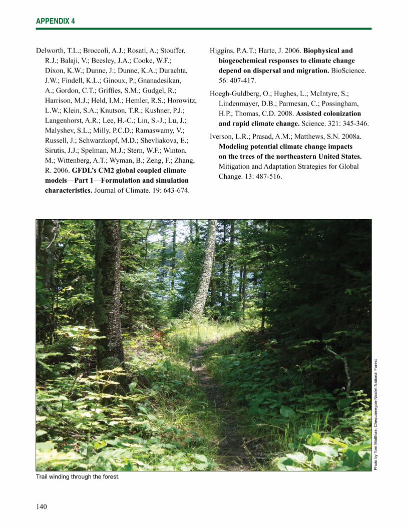
140
APPENDIX 4
Delworth, T.L.; Broccoli, A.J.; Rosati, A.; Stouffer, R.J.; Balaji, V.; Beesley, J.A.; Cooke, W.F.; Dixon, K.W.; Dunne, J.; Dunne, K.A.; Durachta, J.W.; Findell, K.L.; Ginoux, P.; Gnanadesikan, A.; Gordon, C.T.; Griffi es, S.M.; Gudgel, R.; Harrison, M.J.; Held, I.M.; Hemler, R.S.; Horowitz, L.W.; Klein, S.A.; Knutson, T.R.; Kushner, P.J.; Langenhorst, A.R.; Lee, H.-C.; Lin, S.-J.; Lu, J.; Malyshev, S.L.; Milly, P.C.D.; Ramaswamy, V.; Russell, J.; Schwarzkopf, M.D.; Shevliakova, E.; Sirutis, J.J.; Spelman, M.J.; Stern, W.F.; Winton, M.; Wittenberg, A.T.; Wyman, B.; Zeng, F.; Zhang, R. 2006. GFDL’s CM2 global coupled climate models—Part 1—Formulation and simulation characteristics. Journal of Climate. 19: 643-674.
Higgins, P.A.T.; Harte, J. 2006. Biophysical and biogeochemical responses to climate change depend on dispersal and migration. BioScience. 56: 407-417.
Hoegh-Guldberg, O.; Hughes, L.; McIntyre, S.; Lindenmayer, D.B.; Parmesan, C.; Possingham, H.P.; Thomas, C.D. 2008. Assisted colonization and rapid climate change. Science. 321: 345-346.
Iverson, L.R.; Prasad, A.M.; Matthews, S.N. 2008a. Modeling potential climate change impacts on the trees of the northeastern United States. Mitigation and Adaptation Strategies for Global Change. 13: 487-516.
Trail winding through the forest.
Pho
to b
y To
m M
atth
iae,
Che
quam
egon
-Nic
olet
Nat
iona
l For
est
141
APPENDIX 4
Iverson, L.R.; Prasad, A.M.; Matthews, S.N.; Peters, M. 2008b. Estimating potential habitat for 134 eastern US tree species under six climate scenarios. Forest Ecology and Management. 254: 390-406.
Iverson, L.R.; Prasad, A.M.; Schwartz, M.W. 1999. Modeling potential future individual tree-species distributions in the eastern United States under a climate change scenario: a case study with Pinus virginiana. Ecological Modelling. 115: 77-93.
Iverson, L.R.; Schwartz, M.W.; Prasad, A.M. 2004. Potential colonization of new available tree species habitat under climate change: an analysis for fi ve eastern US species. Landscape Ecology. 19: 787-799.
Little, E.L. 1971. Atlas of United States trees. Volume 1. Conifers and important hardwoods. Misc. Publ. 1146. Washington, DC: U.S. Department of Agriculture, Forest Service.
Nakicenovic, N.; Alcamo, J.; Davis, G.; de Vries, B.; Fenhann, J.; Gaffi n, S.; Gregory, K.; Grübler, A.; et al. 2000. IPCC special report on emissions scenarios. Cambridge, United Kingdom: Cambridge University Press. 599 p.
Nowacki, G.J.; Abrams, M.D. 2008. The demise of fi re and “mesophication” of forests in the eastern United States. BioScience. 58: 123-138.
Poland, T.M.; McCullough, D.G. 2006. Emerald ash borer: Invasion of the urban forest and the threat to North America’s ash resource. Journal of Forestry. 104: 118-124.
Pope, V.D. 2000. The impact of new physical parameterizations in the Hadley Centre climate model -- HadCM3. Climate Dynamics. 16: 123-146.
Prasad, A.M.; Iverson, L.R.; Liaw, A. 2006. Newer classifi cation and regression tree techniques: bagging and random forests for ecological prediction. Ecosystems. 9: 181-199.
Prasad, A.M.; Iverson, L.R.; Matthews, S.N.; Peters, M. 2007. A climate change atlas for 134 forest tree species of the eastern United States [Database]. Delaware, OH: U.S. Department of Agriculture, Forest Service, Northern Research Station. Available at http://www.nrs.fs.fed.us/atlas/tree/. (Accessed Feb. 23, 2011).
Schwartz, M.W.; Iverson, L.R.; Prasad, A.M. 2001. Predicting the potential future distribution of four tree species in Ohio, USA, using current habitat availability and climatic forcing. Ecosystems. 4: 568-581.
Schwartz, M.W.; Iverson, L.R.; Prasad, A.M.; Matthews, S.N.; O’Connor, R.J. 2006. Predicting extinctions as a result of climate change. Ecology. 87: 1611-1615.
Vitt, P.; Havens, K.; Kramer, A.; Sollenberger, D.; Yates, E. 2010. Assisted migration of plants: changes in latitudes, changes in attitudes. Biological Conservation. 143(1): 18-27.
Washington, W.M.; Weatherly, J.W.; Meehl, G.A.; Semtner, A.J., Jr.; Bettge, T.W.; Craig, A.P.; Strand, W.G., Jr.; Arblaster, J.M.; Wayland, V.B.; James, R.; Zhang, Y. 2000. Parallel climate model (PCM) control and transient simulations. Climate Dynamics. 16: 755-774.
Webb, T.I. 1992. Past changes in vegetation and climate: lessons for the future. In: Peters, R.L.; Lovejoy, T.E., eds. Global warming and biological diversity. New Haven, CT: Yale University Press: 59-75.
Webb, T.I.; Bartlein, P.J.; Kutzback, J.E. 1987. Climatic change in eastern North America during the past 18,000 years; comparisons of pollen data with model results. In: Ruddiman, W.F.; Wright, H.E.J., eds. North America and adjacent oceans during the last deglaciation. Boulder, CO: The Geological Society of America: 447-462.
Woodall, C.; Oswalt, C.M.; Westfall, J.A.; Perry, C.H.; Nelson, M.D.; Finley, A.O. 2009. An indicator of tree migration in forests of the eastern United States. Forest Ecology and Management. 257: 1434-1444.
142
Abbreviations and AcronymsATFS American Tree Farm SystemATV All-Terrain VehicleCCSP Climate Change Science ProgramCFC Chlorofl uorocarbonCNNF Chequamegon-Nicolet National ForestCOF Council of ForestryFCL Forest Crop LawFIA Forest Inventory and Analysis (USDA Forest Service)FSC Forest Stewardship CouncilGCM General Circulation ModelHFC Hydrofl ourocarbonIPCC Intergovernmental Panel on Climate ChangeMFL Managed Forest LawNASA National Aeronautics and Space AdministrationNOAA National Oceanic and Atmospheric AdministrationNRC Natural Resource CouncilRFSS Regional Forester Sensitive Species SDM Species Distribution ModelSFI Sustainable Forestry InitiativeSRES Special Report on Emissions Scenarios (IPCC 2000)UCS Union of Concerned ScientistsUSCB United States Census BureauUSDA FS United States Department of Agriculture, Forest Service USDA NASS United States Department of Agriculture, National Agricultural Statistics ServiceUSGCRP United States Global Climate Research ProgramUV UltravioletUWM University of Wisconsin-MadisonWDNR Wisconsin Department of Natural ResourcesWDOA Wisconsin Department of AdministrationWDOR Wisconsin Department of RevenueWDWD Wisconsin Department of Work DevelopmentWICCI Wisconsin Initiative on Climate Change ImpactsWISCLAND Wisconsin Initiative for Statewide Cooperation on Landscape Analysis and DataWMO World Meteorological OrganizationWNHI Wisconsin Natural Heritage Inventory
Units of Measurecfsm cubic feet per second per square mileGtCO2eq gigatons of carbon dioxide equivalentppb parts per billionppm parts per million°F degrees Fahrenheit°C degrees Celsius

The U.S. Department of Agriculture (USDA) prohibits discrimination in all its programs and activities on the basis of race, color, national origin, sex, religion, age, disability, political beliefs, sexual orientation, and marital or family status. (Not all prohibited bases apply to all programs.) Persons with disabilities who require alternative means for communication of program information (Braille, large print, audiotape, etc.) should contact USDA’s TARGET Center at 202-720-2600 (voice and TDD). To fi le a complaint of discrimination, write USDA, Director, Offi ce of Civil Rights, Room 326-W, Whitten Building, 1400 Independence Avenue SW, Washington, DC 20250-9410 or call 202-720-5964 (voice and TDD). USDA is an equal opportunity provider and employer.
Printed on recycled paper
Swanston, Chris; Janowiak, Maria; Iverson, Louis; Parker, Linda; Mladenoff, David; Brandt, Leslie; Butler, Patricia; St. Pierre, Matt; Prasad, Anantha; Matthews, Stephen; Peters, Matthew; Higgins, Dale; Dorland, Avery. 2011. Ecosystem vulnerability assessment and synthesis: a report from the Climate Change Response Framework Project in northern Wisconsin. Gen. Tech. Rep. NRS-82. Newtown Square, PA: U.S. Department of Agriculture, Forest Service, Northern Research Station. 142 p.
The forests of northern Wisconsin will likely experience dramatic changes over the next 100 years as a result of climate change. This assessment evaluates key forest ecosystem vulnerabilities to climate change across northern Wisconsin under a range of future climate scenarios. Warmer temperatures and shifting precipitation patterns are expected to infl uence ecosystem drivers and increase stressors, including more frequent disturbances and increased amount or severity of pests and diseases. Forest ecosystems will continue to adapt to changing conditions. Identifying vulnerable species and forests can help landowners, managers, regulators, and policymakers establish priorities for management and monitoring.
KEY WORDS: Climate change, forests, vulnerability, Wisconsin, tree species distributions, Climate Change Atlas, LANDIS-II

www.nrs.fs.fed.us