ecosystem subsidies: terrestrial support of aquatic food webs from

2737

Ecology, 86(10), 2005, pp. 2737–2750q 2005 by the Ecological Society of America

ECOSYSTEM SUBSIDIES: TERRESTRIAL SUPPORT OF AQUATIC FOODWEBS FROM 13C ADDITION TO CONTRASTING LAKES

STEPHEN R. CARPENTER,1,6 JONATHAN J. COLE,2 MICHAEL L. PACE,2 MATTHEW VAN DE BOGERT1,2

DARREN L. BADE,1,2 DAVID BASTVIKEN,3 CAITLIN M. GILLE,1 JAMES R. HODGSON,4 JAMES F. KITCHELL,1

AND EMMA S. KRITZBERG5

1Center for Limnology, University of Wisconsin, Madison, Wisconsin 53706 USA2Institute of Ecosystem Studies, Millbrook, New York 12545 USA

3Department of Water and Environmental Studies, Linkoping University, SE 581 83, Linkoping, Sweden4Department of Biology, St. Norbert College, De Pere, Wisconsin 54115 USA5Department of Ecology/Limnology, Lund University, S-223 62, Lund, Sweden

Abstract. Whole-lake additions of dissolved inorganic 13C were used to measure al-lochthony (the terrestrial contribution of organic carbon to aquatic consumers) in twounproductive lakes (Paul and Peter Lakes in 2001), a nutrient-enriched lake (Peter Lake in2002), and a dystrophic lake (Tuesday Lake in 2002). Three kinds of dynamic models wereused to estimate allochthony: a process-rich, dual-isotope flow model based on mass bal-ances of two carbon isotopes in 12 carbon pools; simple univariate time-series modelsdriven by observed time courses of d13CO2; and multivariate autoregression models thatcombined information from time series of d13C in several interacting carbon pools. Allthree models gave similar estimates of allochthony. In the three experiments without nutrientenrichment, flows of terrestrial carbon to dissolved and particulate organic carbon, zoo-plankton, Chaoborus, and fishes were substantial. For example, terrestrial sources accountedfor more than half the carbon flow to juvenile and adult largemouth bass, pumpkinseedsunfish, golden shiners, brook sticklebacks, and fathead minnows in the unenriched ex-periments. Allochthony was highest in the dystrophic lake and lowest in the nutrient-enriched lake. Nutrient enrichment of Peter Lake decreased allochthony of zooplanktonfrom 0.34–0.48 to 0–0.12, and of fishes from 0.51–0.80 to 0.25–0.55. These experimentsshow that lake ecosystem carbon cycles, including carbon flows to consumers, are heavilysubsidized by organic carbon from the surrounding landscape.

Key words: allochthonous; allochthony; consumer; dissolved inorganic carbon; food web; lake;models; organic carbon; stable isotope; subsidy; whole-lake experiment.

INTRODUCTION

Microbial and animal consumers frequently use re-sources transported to their habitats from elsewhere.These allochthonous resources or subsidies influencepopulation dynamics, community interactions, and eco-system processes (Polis et al. 1997, 2004). There isgrowing evidence for the significance of cross-bound-ary inputs and subsidies of populations in a wide rangeof habitats, including streams, rivers, lakes, islands andriparian terrestrial environments (Kitchell et al. 1999,Fausch et al. 2002, Power and Dietrich 2002, Polis etal. 2004). Allochthonous inputs are a major componentof organic carbon (C) budgets for streams and rivers(Fisher and Likens 1972). More recent studies havedocumented the varying contributions of allochthonousand autochthonous organic carbon sources to consum-ers in a wide range of flowing-water ecosystems (Web-ster and Meyer 1997, Fausch et al. 2002, Power andDietrich 2002, Bunn et al. 2003).

Manuscript received 19 August 2004; revised 2 February2005; accepted 2 March 2005; final version received 12 April2005. Corresponding Editor: A. S. Flecker.

6 E-mail: [email protected]

The importance of subsidies to consumers is alsoimplied by measurements of ecosystem metabolism.Respiration exceeds primary production in many eco-systems, indicating significant input and degradationof allochthonous material. For example, many lakesreceive high loadings of dissolved and particulate or-ganic matter from adjacent wetlands and uplands(Wetzel 1995). As a consequence, in these lakes eco-system respiration commonly exceeds gross primaryproduction (Cole et al. 2000). Thus terrestrial materialsubsidizes lake metabolism. However, the significanceof these subsidies to the support of food webs is lesscertain.

The relative importance of allochthonous vs. au-tochthonous resources cannot be discerned from or-ganic carbon budgets alone. Hence there are few ex-amples where direct estimates have been made of theautochthonous and allochthonous support of food webconstituents. An obvious way to overcome this problemis to trace the flow of allochthonous and autochthonousmatter into food webs using stable isotopes (Kling etal. 1992, France et al. 1997). Where there is a contrastbetween the stable isotope content of sources, it is pos-

2738 STEPHEN R. CARPENTER ET AL. Ecology, Vol. 86, No. 10

TABLE 1. Means of limnological variables from late May to early September for each lake13C addition.

Variable Paul 2001 Peter 2001 Peter 2002 Tuesday 2002

Temperature (8C at 1 m) 21.1 21.4 22.1 22.0Thermocline (m) 3.5 3.6 3.1 2.6pH 6.4 6.9 8.5 6.1Color (m21) 1.5 1.3 1.7 3.5Secchi (m) 4.6 4.9 1.9 2.3pCO2 (matm)† 1039 673 152 977DIC (mmol) 93 141 67 70DOC (mmol) 304 376 483 700POC (mmol) 35.5 34.1 152.3 76.5Chlorophyll a (mg/L) 4.21 3.55 42.1 6.8TP (mmol) 0.314 0.261 0.846 0.385TN (mmol) 26.9 30.3 46.7 28.5GPP (mmol O2·m22·d21) 43.4 31.3 104.5 42.9R (mmol O2·m22·d21) 51.8 31 79.7 44.7

Notes: Variables are as follows: pCO2, partial pressure of CO2; DIC, dissolved inorganiccarbon; DOC, dissolved organic carbon; POC, particulate organic carbon; TP, total phosphorus;TN, total nitrogen; GPP, gross primary production; R, respiration. Chemical measurements aremeans for the epilimnion. Most means were calculated from weekly samples except GPP andR (daily), and POC in 2001, where more frequent samples were taken.

† We report partial pressure as matm. Using the standard atmosphere conversion, a pCO2

value of 1000 matm 5 101.325 3 1023 kPa.

sible to estimate the fraction of consumer carbon flowsupported by each using end-member mixing models.For terrestrial and aquatic primary production, somestudies have compared components of the food web tothese two extremes (Meili et al. 1996, France et al.1997, Jones et al. 1999, Grey et al. 2001). A commonlimitation with these natural abundance studies, how-ever, is the small contrast between terrestrial and aquat-ic primary producers. When these end-member valuesare close, carbon sources to the food web cannot beresolved (Schiff et al. 1990, Cole et al. 2002).

Whole-lake additions of radioactive 14C demonstratethat it is possible to unambiguously label carbon thatis autotrophically fixed within the ecosystem (Hesse-lein et al. 1980, Bower et al. 1987). We have extendedthis approach using the stable isotope 13C. We measuredthe contribution of internal primary production (au-tochthony) to food webs by altering the 13C of dissolvedinorganic carbon (DIC), thereby enriching the 13C ofin-lake primary production relative to organic matterfrom terrestrial inputs (Cole et al. 2002). In many lakesthe isotopic composition of the CO2 moiety of dissolvedinorganic carbon (the proximate substrate for photo-synthesis), and fractionation of that CO2 during pho-tosynthesis, causes carbon fixed by aquatic primaryproducers (especially phytoplankton) to be nearly iden-tical in 13C to organic carbon of terrestrial origin (Karls-son et al. 2003). 13C additions overcome this problemby providing a distinct 13C signature to internal primaryproduction and the consumer carbon derived therefrom.Our previous research used a pulse experiment (Coleet al. 2002) in which a single addition of 13C was made.Press experiments with continuous daily additions of13C allow greater and sustained labeling of the foodweb, reducing immediate losses of 13C to the atmo-

sphere and increasing carbon flows to consumers (Paceet al. 2004).

Although research has begun to quantify the contri-bution of allochthonous carbon to lake food webs, itis not clear how the importance of terrigenous organiccarbon varies among lake consumers and among laketrophic types. In this paper, we use press additions ofDI13C to estimate the terrestrial subsidy to lake eco-systems and specific consumers. This paper adds toresults presented by Pace et al. (2004) by (1) testingwhether terrestrial subsidies are more important in alake with high concentrations of terrestrially deriveddissolved organic matter (DOC) than in a lake with lowconcentrations of terrestrially derived DOC, (2) usinga whole-lake manipulation to test whether the impor-tance of terrestrial subsidies is diminished by nutrientenrichment, (3) comparing allochthony among severaldifferent groups of consumers, and (4) using three dif-ferent modeling approaches to evaluate the consistencyof estimates of allochthony.

METHODS

Inorganic 13C was added to Paul, Peter, and TuesdayLakes located at the University of Notre Dame Envi-ronmental Research Center near Land O’Lakes, Wis-consin, USA (898329 W, 468139 N). These lakes havebeen described in detail (Carpenter and Kitchell 1993),and we focus here mainly on pertinent ecological con-ditions during the 13C additions of 2001 and 2002. Allthree basins are small (0.9–2.5 ha) and steep sided.Lakes are fringed by wetlands and forests typical ofthe upper Great Lakes region. The lakes are all softwater with moderate to high dissolved organic C (DOC)and dissolved inorganic C (DIC), from 80 to 140 mmolamong the three systems (Table 1).

October 2005 2739ALLOCHTHONOUS SUPPORT OF LAKE FOOD WEBS

DOC in the lakes is rich in chromophoric com-pounds; hence lakes in this region with high DOC typ-ically have dark water. Water color measured as theabsorbance of light at 440 nm (Cuthbert and del Giorgio1992) is much higher in Tuesday Lake (2002 average5 3.5 m21) than in Paul (1.5 m21) or Peter (1.3 m21)Lakes. During summer the lakes are strongly stratifiedwith relatively shallow thermocline depths near 3 m(Table 1). Periphyton and phytoplankton are the mainprimary producers, but rates are limited by low nutri-ents (phytoplankton) and low light (periphyton; Car-penter et al. 2001, Vadeboncoeur et al. 2001). Mac-rophytes, while present, are sparse, and do not con-tribute significantly to primary production (Carpenterand Kitchell 1993). The zooplankton community ofPaul Lake is dominated in terms of biomass by largecladocerans (Daphnia spp. and Holopedium gibberum).Peter Lake has a mixture of Daphnia spp., Diaphan-osoma spp., and copepods as biomass dominants. Thezooplankton of Tuesday Lake is an assemblage ofsmall-bodied cladocerans and copepods (Carpenter andKitchell 1993). The planktivorous dipteran, Chaoborusspp., is abundant in Paul and Tuesday Lakes but rarein Peter Lake during 2001 and 2002. The lakes alsodiffer in their fish communities. Paul Lake has onlylargemouth bass (Micropterus salmoides). Peter andTuesday Lakes have mixtures of small-bodied fishes.The dominant species of Peter Lake are pumpkinseeds(Lepomis gibbosus), sticklebacks (Gasterosteus acu-leatus), and fathead minnows (Pimephales promelas).The dominant species of Tuesday Lake are golden shin-ers (Notemigonus crysoleucas), sticklebacks, and fat-head minnows.

In 2001 we added we added 13C in the form ofNaHCO3 (‘‘NaH 13CO3’’) to Paul and Peter Lakes for42 days beginning 11 June and ending 27 July. In 2002we added NaH 13CO3 to Tuesday and Peter Lakes for35 days beginning 17 June and ending 25 July. Eachmorning shortly after dawn, preweighed NaH 13CO3

(99% pure; Isotech, Champaign, Illinois, USA) wasdissolved in lake water within gas-tight carboys. Theresulting solution was pumped into the upper mixedlayer while underway in a boat to promote dispersionof the tracer throughout the mixed layer of the lake.Experiments using rhodamine dye, LiBr, and SF6 inthese lakes indicate that solutes disperse uniformlythrough the mixed layer in ,24 hours (Cole and Pace1998; J. Cole et al., unpublished data). Daily loadingsof NaH 13CO3 were 0.24, 0.35, 0.25, and 0.61 mol 13C/d to Paul (2001), Peter (2001), Tuesday (2002), andPeter (2002) Lakes, respectively. These additions weredesigned to substantially enrich the 13C of DIC whilenot significantly altering total DIC (i.e., 12C 1 13C)concentration. More 13C was added to Peter Lake tocompensate for its higher concentration of DIC and theprospect of substantial inputs of atmospheric 12CO2 in2002 due to nutrient enrichment and chemically en-hanced diffusion (Bade 2004).

In 2002, Peter Lake was also amended with nutrientsto stimulate primary production. Liquid fertilizer wasmade from NH4NO3 and H3PO4. The fertilizer had anatomic nitrogen : phosphorus (N:P) ratio of 25. An ini-tial addition of 0.69 mmol P/m2 and 18.9 mmol N/m2

was made on 3 June 2002 to stimulate primary producergrowth prior to the beginning of the 13C addition. Be-ginning on 10 June and continuing until 25 August,daily additions were made that corresponded to a P-loading rate of 0.11 mmol P·m22·d21 (and 2.7 mmolN·m22·d21). This level of nutrient addition was chosenbecause prior enrichments at this level generated sub-stantial phytoplankton blooms in Peter Lake (Carpenteret al. 2001).

Sampling and measurement of 13C

Detailed methods for most of the measurementsmade in this study are summarized elsewhere (Car-penter et al. 2001, Kritzberg et al. 2004, Pace et al.2004; also available online).7 For this paper we focuson methods to sample and process lake constituents for13C measurements and briefly summarize other mea-surements of physical properties, chemical composi-tion, standing stocks, and rate estimates that supportedmodel analyses. 13C samples for most lake constituentswere taken before, during, and after the tracer addition,at either daily, weekly, or biweekly intervals for fasterand slower C pools.

Particulate organic carbon (POC) and DIC, whichhave fast turnover times, were sampled daily. ForDI13C, water was pumped into gas-tight 60-mL serumvials and acidified to pH 2 with H2SO4. Samples weresent to the University of Waterloo stable isotope facilityand analyzed using a Micromass Isochrome GC-C-IRMS (Waters, Milford, Massachusetts, USA). POCwas concentrated by filtration through precombustedglass fiber filters (GF/F), dried at 408C for 48 h, andacid-fumed to remove excess inorganic 13C. POC andall other particulate samples were analyzed for 13C atthe University of Alaska Isotope Facility using a CarloErba Elemental Analyzer (NC2500; Thermo Electron,Milan, Italy) and a Finnigan MAT Conflo II/III inter-face with a Delta1 Mass Spectrometer (Thermo Elec-tron, Advanced Mass Spectrometry, Bremen, Germa-ny).

Periphyton 13C was sampled weekly by scraping ac-cumulated algae from colonization tiles. Zooplanktonand Chaoborus for isotopic analyses were sampledweekly with oblique net hauls through the upper mixedlayer at night. Individual animals were separated bytaxa under a dissecting microscope, dried, and pulver-ized. Water in filtrates of the POC samples was acidifiedto drive off excess DI13C and concentrated by evapo-ration for isotope analysis of DOC.

Fish were sampled by electrofishing, netting, andangling to obtain animals for isotopic analysis and diet

7 ^http://216.110.136.172/methods.htm&


analysis (Hodgson and Kitchell 1987, Carpenter andKitchell 1993). Gastric lavage was used to obtain gutitems for estimating the isotope content of benthic in-vertebrates (Hodgson and Kitchell 1987). Gut contentswere pooled into diet categories (zooplankton, Chao-borus, largemouth bass young-of-year, and macroin-vertebrates, mainly odonate naiads) for isotope anal-ysis. Invertebrates were also sampled with D-nets, sort-ed by major taxa, dried, ground, and analyzed for 13C.For larger fish, dorsal muscle samples were taken fromthree to five individuals for 13C analysis. For smallerfish, a number of individuals were pooled, dried, pul-verized, and subsampled for 13C analysis.

To obtain samples of bacteria, cultures were grownin situ in dialysis bags using particle-free lake waterand an inoculum of bacteria from the lake (Kritzberget al. 2004). Cells were concentrated on precombustedGF/F filters, dried, and analyzed for 13C using anANCA-NT system and a 20–20 Stable Isotope Ana-lyzer (PDZ Europa, Crewe, Cheshire, UK) at the Ecol-ogy Department, University of Lund, Sweden. Bacte-rial isotope estimates were made four times during eachexperiment.

Isotope data are presented in conventional d notationin per mil units (‰) following the equation d13C 51000 3 [(R/0.011237) 2 1] where R is the ratio of 13Cto 12C in the sample and 0.011237 is the ratio in astandard.

Other measurements

A variety of additional measurements were made toaid interpretation of the isotope dynamics, provide fluxestimates and parameters for modeling analysis, andprovide standing stock estimates for models. DIC,pCO2 (partial pressure of CO2), pH, and temperaturewere measured to calculate the chemical species ofinorganic C and their isotopic content (Mook et al.1974, Zhang et al. 1995). DIC and pCO2 were deter-mined by gas chromatography following establishedmethods (Cole et al. 2000), while pH was measuredwith an electrode (Pace and Cole 2002). Gross primaryproduction and total system respiration were estimatedfrom continuous deployment of YSI sondes (YellowSprings Instrument Company, Yellow Springs, Ohio,USA) that recorded oxygen concentration and temper-ature at 5-min intervals following methods in Cole etal. (2000, 2002) and Hanson et al. (2003). Gas ex-change was estimated from direct measurements of thegas piston velocity (k600) using whole-lake SF6 addi-tions and wind-based estimates from continuous lake-side wind measurements (Wanninkhof et al. 1985, Coleand Caraco 1998). Bacterial production was estimatedfrom leucine incorporation using the microcentrifugetube method (Smith and Azam 1993). Planktonic res-piration was estimated from the decline of oxygen indark bottles (Pace and Cole 2000). Weekly vertical pro-files of temperature, O2, irradiance (photosyntheticallyactive radiation, PAR), and chlorophyll a were made

in each lake to estimate mixed-layer depth and to cal-culate phytoplankton biomass.

Standing stocks of POC and DOC were derived frommixed-layer water samples using a Carlo-Erba C/N an-alyzer and a Shimadzu 5050 TOC analyzer (Shimadzu,Kyoto, Japan) for POC and DOC, respectively. Weeklymeasurements of phytoplankton and zooplankton bio-mass were derived from vertical profiles of chlorophylla and calibrated net hauls, respectively, using methodsdescribed in Carpenter and Kitchell (1993) and Car-penter et al. (2001). Chaoborus were sampled with ver-tical net hauls every week and biomass determinedfrom estimates of abundance and measurements oflength and diameter (Carpenter and Kitchell 1993).

Fish abundance, size distribution, and diets weremeasured using methods described in Hodgson andKitchell (1987) and Carpenter and Kitchell (1993). Es-timates of largemouth bass populations were calculatedby mark–recapture methods using data from electro-shocking and angling (Seber 1982). Fishes were sam-pled weekly using minnow traps in Peter and TuesdayLakes (Carpenter and Kitchell 1993).

Model methods

Changes in d13C over time for the major carbon poolswere used to estimate allochthony, the proportion ofcarbon flow into a pool from terrestrial sources. In thesetracer experiments, information about flows is obtainedfrom transient changes in d13C. Therefore, the steady-state mixing models used in studies of natural isotopeabundance are not appropriate. At present there is nosingle standard method for assessment of carbon fluxesthrough the entire food web in whole-ecosystem tracerexperiments. Many modeling approaches are poten-tially applicable, and we do not know if they will leadto similar or different conclusions. Therefore, we usedthree different modeling approaches. To the extent thatthese give similar results, we can have confidence thatconclusions are robust. The differences among modelresults provide information about the uncertainties thatderive from model selection.

Initially we developed dual isotope flow (DIF) mod-els for each experiment (Appendix A; Cole et al. 2002).The DIF employs mass-balance of total carbon and 13Cfor 12 carbon pools. Many pool sizes and flows weredirectly measured to calibrate the DIF. The DIF pro-vides a detailed analysis that is grounded in the currentunderstanding of the major processes that govern car-bon flows in lake ecosystems. While this is an advan-tage, the DIF depends on a large number and diversityof measurements and could potentially propagate errorsin complicated ways. A complete statistical analysis ofthe DIF is not possible, but we did fit some parametersby least squares, perform numerous sensitivity exper-iments, and evaluate goodness of fit statistics.

To provide a contrast in complexity, we developedunivariate time-series models (Appendix B; Pace et al.2004). These predicted d13C of a response pool (DOC,


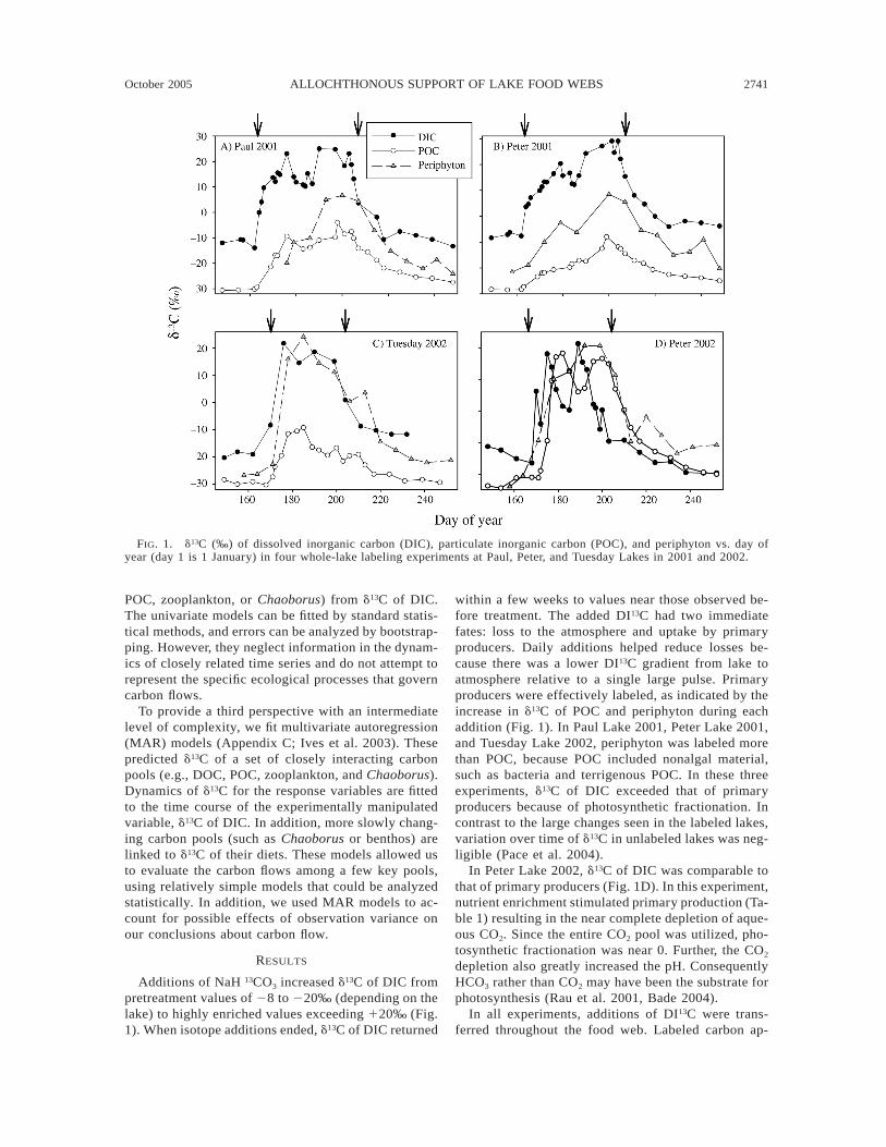
FIG. 1. d13C (‰) of dissolved inorganic carbon (DIC), particulate inorganic carbon (POC), and periphyton vs. day ofyear (day 1 is 1 January) in four whole-lake labeling experiments at Paul, Peter, and Tuesday Lakes in 2001 and 2002.

POC, zooplankton, or Chaoborus) from d13C of DIC.The univariate models can be fitted by standard statis-tical methods, and errors can be analyzed by bootstrap-ping. However, they neglect information in the dynam-ics of closely related time series and do not attempt torepresent the specific ecological processes that governcarbon flows.

To provide a third perspective with an intermediatelevel of complexity, we fit multivariate autoregression(MAR) models (Appendix C; Ives et al. 2003). Thesepredicted d13C of a set of closely interacting carbonpools (e.g., DOC, POC, zooplankton, and Chaoborus).Dynamics of d13C for the response variables are fittedto the time course of the experimentally manipulatedvariable, d13C of DIC. In addition, more slowly chang-ing carbon pools (such as Chaoborus or benthos) arelinked to d13C of their diets. These models allowed usto evaluate the carbon flows among a few key pools,using relatively simple models that could be analyzedstatistically. In addition, we used MAR models to ac-count for possible effects of observation variance onour conclusions about carbon flow.

RESULTS

Additions of NaH 13CO3 increased d13C of DIC frompretreatment values of 28 to 220‰ (depending on thelake) to highly enriched values exceeding 120‰ (Fig.1). When isotope additions ended, d13C of DIC returned

within a few weeks to values near those observed be-fore treatment. The added DI13C had two immediatefates: loss to the atmosphere and uptake by primaryproducers. Daily additions helped reduce losses be-cause there was a lower DI13C gradient from lake toatmosphere relative to a single large pulse. Primaryproducers were effectively labeled, as indicated by theincrease in d13C of POC and periphyton during eachaddition (Fig. 1). In Paul Lake 2001, Peter Lake 2001,and Tuesday Lake 2002, periphyton was labeled morethan POC, because POC included nonalgal material,such as bacteria and terrigenous POC. In these threeexperiments, d13C of DIC exceeded that of primaryproducers because of photosynthetic fractionation. Incontrast to the large changes seen in the labeled lakes,variation over time of d13C in unlabeled lakes was neg-ligible (Pace et al. 2004).

In Peter Lake 2002, d13C of DIC was comparable tothat of primary producers (Fig. 1D). In this experiment,nutrient enrichment stimulated primary production (Ta-ble 1) resulting in the near complete depletion of aque-ous CO2. Since the entire CO2 pool was utilized, pho-tosynthetic fractionation was near 0. Further, the CO2

depletion also greatly increased the pH. ConsequentlyHCO3 rather than CO2 may have been the substrate forphotosynthesis (Rau et al. 2001, Bade 2004).

In all experiments, additions of DI13C were trans-ferred throughout the food web. Labeled carbon ap-


FIG. 2. d13C (‰) predicted by the dual isotope flow (DIF) model (lines) and observed (points) vs. day of year (day 1 is1 January) for Paul Lake in 2001. (A) DIC and POC, (B) DOC and bacteria, (C) periphyton and benthos, (D) zooplankton,(E) Chaoborus, and (F) three size classes of largemouth bass: young-of-year (YOY; solid circles), juveniles (open circles),and adults (solid triangles). Arrows indicate the start and end of the isotope addition.

peared in bacteria shortly after initiation of the 13Caddition (Fig. 2B). DOC was also labeled, though to alesser extent because of the large size of this carbonpool. Although periphyton rapidly accumulated 13C, la-beled carbon accumulated slowly in benthic inverte-brates in this experiment (Fig. 2C).

Zooplankton accumulated 13C shortly after 13C ap-peared in the POC (Fig. 2D), and labeled carbon inzooplankton was transferred to Chaoborus (Fig. 2E).Among fishes of Paul Lake, young-of-year largemouthbass accumulated 13C to the greatest extent, consistentwith their more rapid carbon turnover rate and zoo-planktivorous habit (Fig. 2F). Juvenile largemouth bassaccumulated some 13C as a consequence of eating zoo-plankton, Chaoborus, benthos, and young-of-year bass.Adult largemouth bass were labeled only slightly. Thisresult was predicted by the bass bioenergetics modeland is consistent with the slow carbon turnover rate ofthese large but slow-growing fishes. Both juvenile andadult largemouth bass consume terrestrial prey itemswhich are not enriched in 13C.

The DIF model appeared to fit the observed d13C(Fig. 2 and Appendix D). This model includes a com-prehensive analysis of the carbon cycle by employinga substantial amount of field data on carbon pool sizesand flux rates (Appendix A). That richness of process-

level detail is an advantage. Discrepancies betweenmodel predictions and observations are small relativeto the overall changes in the data. But because so manyobservations must be accommodated simultaneously,there can be systematic departures between predictedand observed d13C. For example, in Paul Lake 2001,the model underestimates labeling of zooplankton andoverestimates labeling of Chaoborus (Fig. 2E, F).

Similar results occurred in the other experiments.Residual standard deviations for most compartmentswere ,1‰, and these deviations were typically smallrelative to the large range of 13C created by the ma-nipulation (Appendix D). Overall, correspondence be-tween observed d13C and predictions of the DIF modelwas similar in all four experiments (Appendix D).

The univariate models focus on one carbon pool ata time predicting dynamics from the DI13C time seriesand a fixed pool of carbon with a terrestrial signatureof 228‰ (Pace et al. 2004). These parsimonious mod-els fit the data closely in most cases, as illustrated forPeter Lake in Fig. 3. The model simulates the increaseand decline of 13C, with the exception of underpre-dicting POC observations in the 2002 experiment atmaximum labeling (Fig. 3). Fits of similar quality werefound for other experiments (Appendix D). The uni-variate models are limited in that fits for a given carbon


FIG. 3. d13C (‰) predicted by univariate models (lines) and observed (points) vs. day of year (day 1 is 1 January) forPeter Lake.

pool do not take advantage of information in closelyrelated carbon pools. Also, dynamics of d13C in slowlychanging pools, such as benthos or fishes, are not easilypredicted from the relatively rapid changes of d13C inDIC and the many transformations that occur as carbonmoves through the food web to these consumers. There-fore we did not attempt to fit univariate models forthese slowly changing pools.

MAR models incorporate additional information byincluding the dynamics of closely related variables.Predictions of the MAR models closely match observedd13C in most cases, as shown in Fig. 4 for Tuesday Lakein 2002. The MAR approach considers three subsys-tems of the food web. The modest response of the ben-thos to the substantial enrichment of periphyton is cap-tured (Fig. 4A). Bacterial 13C falls between POC andDOC but more closely reflects the dynamics of PO13C,reflecting preferential utilization of the autotrophiccomponent of POC (Fig. 4B; Kritzberg et al. 2004).Predicted zooplankton and Chaoborus 13C dynamics fitthe data well, and the MAR model represents the ex-pected lag in labeling of Chaborus relative to their prey(Fig. 4C). Fits of similar quality were found for otherexperiments (Appendix D). We did not attempt to fitMAR models for fishes. Instead we combined MARestimates of allochthony of diet items with data oncomposition of fish diets to calculate allochthony offishes.

Allochthony, the proportion of carbon flow from ter-restrial sources, was calculated for all organic carbonpools in the DIF model, and for as many carbon poolsas could be fitted for the univariate and MAR models

(Table 2). All models indicate that the major carbonpools POC and DOC had significant allochthonouscomponents. For example, in the experiments withoutnutrient enrichment (Paul Lake 2001, Peter Lake 2001,Tuesday Lake 2002) POC allochthony ranged from0.29 to 0.59, depending on the model. In the nutrientenrichment experiment (Peter Lake 2002), allochthonyof POC ranged from 0 to 0.07, depending on the model.Thus nutrient enrichment increased the contribution ofphytoplankton to POC.

DOC was more allochthonous than POC (Table 2).In the unenriched experiments, allochthony of DOCranged from 0.53 to 0.96, depending on the lake andthe model. In dystrophic Tuesday Lake, model esti-mates of DOC allochthony were consistently high(0.92–0.96). For each model, the lowest estimate ofDOC allochthony occurred in the enrichment experi-ment (Peter Lake 2002).

Carbon flow through bacteria was dominated by al-lochthonous sources in the unenriched experiments (al-lochthony range, 0.60–0.76 depending on the modeland experiment). In the enriched experiment, the DIFmodel estimated bacterial allochthony as 0.39, but datawere insufficient for analysis using the other models.

Allochthony of zooplankton was similar in Paul Lakeand Peter Lake in 2001 (0.22–0.48). In Tuesday Lake,zooplankton were more allochthonous (0.49–0.75). InPeter Lake during enrichment in 2002, zooplanktonwere supported almost entirely by within-lake primaryproduction, and allochthony estimates ranged from 0to 0.12. The same general pattern—more allochthony


TABLE 2. Allochthony (proportion of carbon flow from terrestrial sources) for major carbon pools, estimated using threedifferent models.

Lake Year Method DOC Bacteria POC

Paul 2001 DIF 0.53 0.60 0.29Paul 2001 MAR 0.83 6 0.01 0.71 6 0.18 0.38 6 0.03Paul 2001 univar. 0.85 6 0.02 0.40 6 0.03Peter 2001 DIF 0.69 0.73 0.50Peter 2001 MAR 0.87 6 0.01 0.47 6 0.04Peter 2001 univar. 0.87 6 0.01 0.55 6 0.03Peter 2002 DIF 0.43 0.39 0.06Peter 2002 MAR 0.55 6 0.10 0.07 6 0.00Peter 2002 univar. 0.70 6 0.02 0.00 6 0.01Tues 2002 DIF 0.92 0.76 0.48Tues 2002 MAR 0.95 6 0.02 0.67 6 0.04 0.57 6 0.05Tues 2002 univar. 0.96 6 0.01 0.59 6 0.05

Notes: For univariate and multivariate autoregression (MAR) models, bootstrapped standard deviations are presented. InPaul Lake, Fish 1 is young-of-year largemouth bass, Fish 2 is juvenile largemouth bass, and Fish 3 is adult largemouth bass.In Peter Lake, Fish 1 is pumpkinseed, Fish 2 is stickleback, and Fish 3 is fathead minnow. In Tuesday Lake, Fish 1 is goldenshiner, Fish 2 is stickleback, and Fish 3 is fathead minnow. DIF refers to the dual isotope flow model (Appendix A). Otherabbreviations are as in Table 1.

FIG. 4. d13C (‰) predicted by multivariate autoregression(MAR) models (lines) and observed (points) vs. day of year(day 1 is 1 January) for Tuesday Lake in 2002.

in Tuesday Lake, less allochthony in Peter Lake withenrichment—was evident for Chaoborus.

Benthic invertebrates had similar allochthony in theunenriched experiments (0.60–0.85). Benthos tended

to be more allochthonous than zooplankton. Under en-richment, allochthony of benthos appeared to decrease,although the gap between DIF estimates and MAR es-timates was large.

In Paul Lake, flow of carbon to juvenile and adultlargemouth bass (Fishes 2 and 3 in Table 2) was morethan half allochthonous. Diets of these fishes includesubstantial numbers of terrestrial prey (Hodgson andKitchell 1987). Young-of-year largemouth bass wereless allochthonous, partly because these fish feed pri-marily on zooplankton during the first few weeks oflife (Post et al. 1997). In Tuesday Lake, we estimatedhigh allochthony for a different set of fishes: goldenshiner, stickleback, and fathead minnow.

In Peter Lake, allochthony of pumpkinseed sunfish,stickleback, and fathead minnow (Fishes 1, 2, and 3,respectively, in Table 2) declined with nutrient enrich-ment. Prior to enrichment, fish allochthony was com-parable to that of the other lakes (0.51–0.80). Afterenrichment, fish allochthony declined to 0.25–0.55.These results indicate that nutrient enrichment of PeterLake caused a decrease in the contribution of terrige-nous carbon, relative to carbon fixed in the lake, tofishes during the course of the experiment.

DISCUSSION

Evaluation of allochthony estimates

Our experiments label new, autochthonous primaryproduction of phytoplankton and periphyton in themixed layer of the lakes for 35–42 d. The experimentsshow clearly that some portion of secondary productionis directly supported by this contemporaneous, surface-layer, labeled primary production and some is not.Some portion of secondary production may, therefore,be supported by terrestrially derived organic C (allo-chthony) but there are additional possibilities. Con-sumers may utilize contemporaneous primary produc-tion from waters or sediments deeper than the mixed


TABLE 2. Extended.

Zooplankton Chaoborus Benthos Fish 1 Fish 2 Fish 3

0.37 0.37 0.60 0.38 0.59 0.730.24 6 0.04 0.36 6 0.06 0.84 6 0.06 0.67 0.72 0.760.22 6 0.05 0.53 6 0.09

0.34 0.34 0.85 0.69 0.71 0.510.41 6 0.01 0.41 0.78 0.80 0.65 0.540.48 6 0.03

0.12 0.12 0.07 0.40 0.45 0.330.08 6 0.00 0.20 6 0.04 0.41 6 0.11 0.55 0.30 0.250.00 6 0.02 0.12 6 0.08

0.75 0.75 0.83 0.93 0.93 0.840.49 6 0.04 0.49 6 0.04 0.72 6 0.23 0.56 0.65 0.580.74 6 0.04 0.65 6 0.56

layer that is not labeled with added 13C. Alternatively,consumers may consume detritus from primary pro-duction that occurred prior to the time 13C was added.Several lines of evidence suggest that these processesare not important in these experiments. We evaluatethis evidence for POC and DOC inputs to the epilim-nion, for vertical migration and feeding of planktonicorganisms, and for sources of C consumed by epilim-netic benthos.

POC inputs.—The three study lakes are stronglystratified during summer. Solutes added to the uppermixed layer do not move across the thermocline (seeCole and Pace 1998, Houser 2001). There is no mech-anism, except thermocline deepening, that can addDOC or POC from below the thermocline to the mixedlayer. For POC, the DIF and MAR models calculatethat losses of epilimnetic POC from sedimentation andconsumption are rapid, and hence the epilimnetic POCpool turns over in a few days. In the case of POC, thestanding stock is replaced many times over the courseof the experiment, and its 13C content represents theintroduction of new inputs. In addition to autochtho-nous primary production, the possible inputs of newPOC include flocculation of DOC (which the DIF mod-el accounts for), terrestrial inputs (accounted for), andresuspension of previously deposited material on epi-limnetic sediments. To the extent that a portion of thisresuspended material could be both autochthonous inorigin and older than the experiment, our estimate ofallochthony for POC might be compromised. A simplecalculation suggests that the total amount of resuspen-sion from these sediments could be only a trivial por-tion of the POC input to the epilimnion. Using the MARmodel, POC inputs can be estimated as daily turnover3 allochthony 3 mean areal density of POC (AppendixC). Estimated POC inputs during the experiments were62 mg·m22·d21 in Paul Lake, 47 mg·m22·d21 in PeterLake 2001, 35 mg·m22·d21 in Peter Lake 2002, and 104mg·m22·d21 in Tuesday Lake. Epilimnetic sedimentscomprise ;10% of the surface area of these lakes. If10% of annual primary production were deposited onthese sediments, only 50% of this decomposed in place,

and all of the rest was resuspended into the lake duringthe ice-free season, resuspension of autochthonous ma-terial would supply ,5 mg C·m22·d21 (to the wholelake), which is much smaller than the required POCinput to the water column. This calculation of resus-pended POC is certainly an overestimate in these smalllakes, which experience little wave action and low re-suspension of sediments. We conclude that epilimneticPOC was primarily derived from autochthonous pri-mary production and new terrestrial inputs during thecourse of the manipulations.

Origins of DOC.—DOC is a mixture of both au-tochthonous and allochthonous sources, and the aver-age pool turns over slowly, ;3%/d (Bade 2004). CouldDOC produced autochthonously prior to the experi-ment compromise our interpretation of allochthony?Kritzberg et al. (2004) demonstrated that bacteria pref-erentially utilize DOC of fresh algal origin in the studylakes, and this preference is accounted for in the DIFmodel. This preference rapidly depletes much of thefresh DOC of algal origin from the DOC standing stock.Bade (2004), using a kinetic modeling approach, es-timates that, except for the nutrient-enriched lake (Peter2002), terrestrial DOC comprises from 80 to 90% ofthe DOC standing stock, in agreement with the resultspresented here (Table 1). Thus while there is both al-lochthonous and autochthonous input to the DOC pool,these findings imply that most of the bulk standingstock DOC at any point in time is terrestrial in origin(as is the case for many lakes, Hessen and Tranvik1998). Thus any effects of older DOC derived fromphytoplankton are minor. In the case of the nutrient-enriched lake (Peter 2002) as much as 40% of the DOCpool is of algal origin (Bade 2004). In this case, how-ever, the nutrients and the 13C were added in the sameseason, precluding a large role for algal DOC producedprior to the experiment. We conclude that DOC wasprimarily allochthonous and not transiently enriched inautochthonous carbon prior to the 13C additions. Usingthe MAR model, DOC input rates can be estimated asdaily turnover 3 allochthony 3 mean areal density ofDOC (Appendix C). Estimated input rates during the


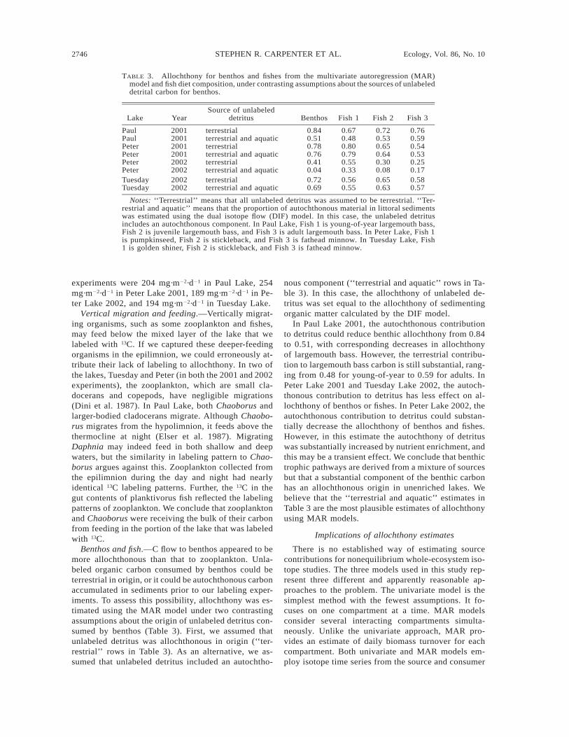
TABLE 3. Allochthony for benthos and fishes from the multivariate autoregression (MAR)model and fish diet composition, under contrasting assumptions about the sources of unlabeleddetrital carbon for benthos.

Lake YearSource of unlabeled

detritus Benthos Fish 1 Fish 2 Fish 3

Paul 2001 terrestrial 0.84 0.67 0.72 0.76Paul 2001 terrestrial and aquatic 0.51 0.48 0.53 0.59Peter 2001 terrestrial 0.78 0.80 0.65 0.54Peter 2001 terrestrial and aquatic 0.76 0.79 0.64 0.53Peter 2002 terrestrial 0.41 0.55 0.30 0.25Peter 2002 terrestrial and aquatic 0.04 0.33 0.08 0.17Tuesday 2002 terrestrial 0.72 0.56 0.65 0.58Tuesday 2002 terrestrial and aquatic 0.69 0.55 0.63 0.57

Notes: ‘‘Terrestrial’’ means that all unlabeled detritus was assumed to be terrestrial. ‘‘Ter-restrial and aquatic’’ means that the proportion of autochthonous material in littoral sedimentswas estimated using the dual isotope flow (DIF) model. In this case, the unlabeled detritusincludes an autochthonous component. In Paul Lake, Fish 1 is young-of-year largemouth bass,Fish 2 is juvenile largemouth bass, and Fish 3 is adult largemouth bass. In Peter Lake, Fish 1is pumpkinseed, Fish 2 is stickleback, and Fish 3 is fathead minnow. In Tuesday Lake, Fish1 is golden shiner, Fish 2 is stickleback, and Fish 3 is fathead minnow.

experiments were 204 mg·m22·d21 in Paul Lake, 254mg·m22·d21 in Peter Lake 2001, 189 mg·m22·d21 in Pe-ter Lake 2002, and 194 mg·m22·d21 in Tuesday Lake.

Vertical migration and feeding.—Vertically migrat-ing organisms, such as some zooplankton and fishes,may feed below the mixed layer of the lake that welabeled with 13C. If we captured these deeper-feedingorganisms in the epilimnion, we could erroneously at-tribute their lack of labeling to allochthony. In two ofthe lakes, Tuesday and Peter (in both the 2001 and 2002experiments), the zooplankton, which are small cla-docerans and copepods, have negligible migrations(Dini et al. 1987). In Paul Lake, both Chaoborus andlarger-bodied cladocerans migrate. Although Chaobo-rus migrates from the hypolimnion, it feeds above thethermocline at night (Elser et al. 1987). MigratingDaphnia may indeed feed in both shallow and deepwaters, but the similarity in labeling pattern to Chao-borus argues against this. Zooplankton collected fromthe epilimnion during the day and night had nearlyidentical 13C labeling patterns. Further, the 13C in thegut contents of planktivorus fish reflected the labelingpatterns of zooplankton. We conclude that zooplanktonand Chaoborus were receiving the bulk of their carbonfrom feeding in the portion of the lake that was labeledwith 13C.

Benthos and fish.—C flow to benthos appeared to bemore allochthonous than that to zooplankton. Unla-beled organic carbon consumed by benthos could beterrestrial in origin, or it could be autochthonous carbonaccumulated in sediments prior to our labeling exper-iments. To assess this possibility, allochthony was es-timated using the MAR model under two contrastingassumptions about the origin of unlabeled detritus con-sumed by benthos (Table 3). First, we assumed thatunlabeled detritus was allochthonous in origin (‘‘ter-restrial’’ rows in Table 3). As an alternative, we as-sumed that unlabeled detritus included an autochtho-

nous component (‘‘terrestrial and aquatic’’ rows in Ta-ble 3). In this case, the allochthony of unlabeled de-tritus was set equal to the allochthony of sedimentingorganic matter calculated by the DIF model.

In Paul Lake 2001, the autochthonous contributionto detritus could reduce benthic allochthony from 0.84to 0.51, with corresponding decreases in allochthonyof largemouth bass. However, the terrestrial contribu-tion to largemouth bass carbon is still substantial, rang-ing from 0.48 for young-of-year to 0.59 for adults. InPeter Lake 2001 and Tuesday Lake 2002, the autoch-thonous contribution to detritus has less effect on al-lochthony of benthos or fishes. In Peter Lake 2002, theautochthonous contribution to detritus could substan-tially decrease the allochthony of benthos and fishes.However, in this estimate the autochthony of detrituswas substantially increased by nutrient enrichment, andthis may be a transient effect. We conclude that benthictrophic pathways are derived from a mixture of sourcesbut that a substantial component of the benthic carbonhas an allochthonous origin in unenriched lakes. Webelieve that the ‘‘terrestrial and aquatic’’ estimates inTable 3 are the most plausible estimates of allochthonyusing MAR models.

Implications of allochthony estimates

There is no established way of estimating sourcecontributions for nonequilibrium whole-ecosystem iso-tope studies. The three models used in this study rep-resent three different and apparently reasonable ap-proaches to the problem. The univariate model is thesimplest method with the fewest assumptions. It fo-cuses on one compartment at a time. MAR modelsconsider several interacting compartments simulta-neously. Unlike the univariate approach, MAR pro-vides an estimate of daily biomass turnover for eachcompartment. Both univariate and MAR models em-ploy isotope time series from the source and consumer


compartments, and no other rate measurements. Errorestimates for univariate and MAR models are easilycomputed by bootstrapping. The DIF model, in con-trast, uses many field measurements of ecosystem rates,all available isotope time series, and many assumptionsabout ecosystem structure and feedbacks. This addedcomplexity allows the DIF model to estimate more flux-es among ecosystem compartments than the other mod-els, thereby providing a more detailed breakdown ofecosystem carbon flows. It is not possible to computea statistically rigorous estimate of errors for the DIFmodel. However, errors in predicting d13C were similarfor the three models (Appendix D).

In general there was good agreement among the threemodels, with the univariate and MAR models produc-ing the most similar estimates. The correspondence ofthese two approaches results partly from the impor-tance of the time-series data of the focal compartmentcommon to both estimates. DIF model estimates dif-fered in some cases from the univariate and MAR mod-els, but these differences were usually not consistentwhen results were compared among lakes. For exam-ple, DIF model estimates of zooplankton allochthonywere 15% higher than the univariate model for PaulLake in 2001, but this difference was reversed for PeterLake 2001 where the DIF model estimate was 14%lower than the univariate model. Hence we concludethat the differences among allochthony estimates forzooplankton largely reflect model uncertainty. The DIFmodel consistently produced lower estimates of the au-tochthonous contribution to DOC than the univariateand MAR estimates. Except in Tuesday Lake, the DIFmodel indicates DOC has a significant autochthonouscomponent in contrast with the other two models. Thisdiscrepancy suggests that autochthonous fluxes by anumber of mechanisms (phytoplankton release, phy-toplankton mortality, consumer release) are importantand not well captured by the indirect, empirical ap-proaches of the MAR and univariate models. If the DIFmodel estimates are more realistic, additional study ofthese mechanisms is warranted, especially in terms ofhow these sources produce autochthonous DOC thataccumulates.

All three models indicate that allochthony was sub-stantial. Carbon flow to ‘‘herbivorous’’ zooplanktonwas 22–75% allochthonous in unenriched lakes, due toconsumption of terrigenous POC and bacterial carbonderived from terrigenous DOC. Carbon flow to fisheswas more allochthonous than that to zooplankton (fora given model). Fish allochthony is higher, because ofgreater reliance on allochthonous benthic resources anddirect consumption of terrestrial prey (Hodgson andKitchell 1987). Allochthonous organic carbon repre-sents a substantial subsidy to food webs of these lakes.

Many ecosystems receive substantial inputs of or-ganic carbon from outside their boundaries. Ecologistshave only recently begun to evaluate the contributionof these carbon inputs to food webs. In a number of

cases, species populations or consumer guilds are sub-sidized by exogenous food sources (Polis et al. 1997,2004). Our experiments demonstrate substantial organ-ic carbon subsidies to entire food webs of ecosystems.This finding is not consistent with the simplificationoften made for lakes where the food web is viewed aslargely supported by endogenous primary production.Instead, lake ecosystems, such as stream ecosystems(Wallace et al. 1997, Nakano and Murakami 2001), areopen, and consumers derive significant amounts of car-bon from exogenous sources.

Allochthony is reduced if nutrients are added. Therelative importance of allochthonous carbon flow to allconsumers decreased as a result of nutrient enrichmentof Peter Lake. This result is consistent with an earlierpulse labeling experiment of an entire lake, in whichnutrients were added and zooplankton were found tobe supported largely by autochthonous carbon (Cole etal. 2002). Eutrophication results from increased flowof nutrients from land to lakes, but the increase inautochthonous primary production reduces the depen-dency of aquatic consumers on terrigenous organic car-bon. Thus changes in landscapes that increase nutrientflow to lakes, such as land conversion for agricultureor urbanization (Carpenter et al. 1998), may reduce theterrestrial subsidy of organic matter to aquatic con-sumers and thereby decouple the aquatic food web fromits watershed.

Terrigenous subsidies were more important in dys-trophic Tuesday Lake than in the other lakes. Changesin landscapes that increase the flux or concentration ofterrigenous organic matter in lakes (Canham et al.2004) may increase the terrestrial subsidy to aquaticfood webs. The relative importance of terrestrial sub-sidies may wax or wane over decades to millennia aschanges in hydrology, soils, and watershed vegetationalter nutrient and organic matter inputs to lakes.

Allochthony is related to color : chlorophyll a ratio,which is an easily measured index of terrigenous or-ganic carbon relative to endogenous producer biomass(Fig. 5). Means of the three models represent our bestestimate of allochthony for four consumer compart-ments, and ranges represent the variability among mod-els (Table 2 for zooplankton and Chaoborus from allmodels, Table 2 for benthos and fish from DIF model,Table 3 for benthos and fish from MAR model). Allincrease with the color : chlorophyll a ratio except ben-thos, where allochthony is high for three of four cases.A similar positive relationship between percent allo-chthony and the ratio of color : chlorophyll a also oc-curs for the two major pelagic C pools, DOC and POC(data not shown). Color (light absorbance at 440 nm)is a measure of chromophoric dissolved organic matter(CDOM), which is largely of terrestrial origin (Hessenand Tranvik 1998). CDOM is probably proportional tothe amount of terrestrially derived organic C potentiallyavailable to consumers in a given lake. Chlorophyll ais proportional to phytoplankton biomass, an index of


FIG. 5. Allochthony (the proportion of carbon flow fromterrestrial sources) vs. ratio of color to chlorophyll a for (A)zooplankton, (B) Chaoborus (not available in Peter Lake2001), (C) benthos, (D) fish (YOY bass in Paul Lake 2001,fathead minnows in the other three experiments). Symbolsshow the means, and error bars show the maximum and min-imum values observed. Experiments in order of color : chlo-rophyll are: Peter Lake 2002, Paul Lake, Peter Lake 2001,Tuesday Lake.

the amount of autochthonous C potentially available toconsumers. Allochthony is inversely related to primaryproducer biomass and positively related to terrestriallyderived CDOM. While allochthony in our experimentsalso tracks other measures of autochthonous primaryproduction and terrestrial C-loading (e.g., measuredgross primary production and estimated terrestrial in-puts of DOC), color and chlorophyll a data are widelyavailable for a large number of lakes and may ulti-mately prove to be a useful predictor of allochthony.Because few measurements of whole-ecosystem allo-chthony are available, other variables such as lake size,morphometry, or water residence time may also be im-portant.

There is long history of research on material fluxesfrom land to water in ecosystem ecology (Likens andBormann 1974). More recently, ecologists have ad-dressed the role of cross-boundary subsidies for pop-ulation and community ecology (Polis et al. 2004). Inorder to be important for the receiving ecosystem,cross-boundary fluxes must be used by consumers inthat ecosystem. Our experiments show that consumerproduction in small, relatively unproductive lakes isheavily subsidized by organic carbon from the sur-rounding landscape. The importance of this subsidy isreduced by nutrient enrichment, and is greater in adystrophic lake with high concentrations of terrigenousDOC.

Our experimental lakes are near the average size forthe Northern Highland Lake District (median area, 0.33ha; range, 0.008 to 1625 ha; n 5 6928; North TemperateLakes Long-Term Ecological Research site; S. Car-penter et al., unpublished data). However, a substantialproportion of the landscape’s lake area and fresh-watervolume is found in larger lakes. The importance ofterrigenous organic carbon in larger lakes is uncertain.Inputs at the perimeter may be simply diluted in largerlakes, leading to the expectation that autochthonydrives the lake food web. Alternatively, consumers mayorient toward the littoral zone, a highly productive eco-tone (Schindler and Scheuerell 2002, Vander Zandenand Vadeboncoeur 2002), and thereby remain highlydependent on terrigenous carbon even in larger lakes.

ACKNOWLEDGMENTS

We thank Jon Frum for guidance and inspiration. The Uni-versity of Notre Dame Environmental Research Center andits director, Gary Belovsky, helped make this research pos-sible. Technical assistance was provided by Robert Drimme,Crystal Fankhouser, Norma Haubenstock, Jefferson Hinke,and Molli MacDonald. ISOTEC, especially B. Montgomery,facilitated our purchase of a large amount of 13C. We aregrateful for the financial support of the National ScienceFoundation and the Andrew W. Mellon Foundation.

LITERATURE CITED

Bade, D. L. 2004. Ecosystem carbon cycles: whole-lake flux-es estimated with multiple isotopes. Dissertation. Univer-sity of Wisconsin, Madison, Wisconsin, USA.

Bower, P. M., C. A. Kelly, E. J. Fee, J. Shearer, and D. R.DeClerq. 1987. Simultaneous measurement of primaryproduction by whole-lake and bottle radiocarbon additions.Limnology and Oceanography 32:299–312.

Bunn, S. E., P. M. Davies, and M. Winning. 2003. Sourcesof organic carbon supporting the food web of an arid flood-plain river. Freshwater Biology 48:619–635.

Canham, C. D., M. L. Pace, M. J. Papaik, A. G. B. Primack,K. M. Roy, R. J. Maranger, R. P. Curran, and D. M. Spada.2004. A spatially-explicit watershed-scale analysis of dis-solved organic carbon in Adirondack lakes. Ecological Ap-plications 14:839–854.

Carpenter, S. R., N. F. Caraco, D. L. Correll, R. W. Howarth,A. N. Sharpley, and V. H. Smith. 1998. Nonpoint pollutionof surface waters with phosphorus and nitrogen. EcologicalApplications 8:559–568.

Carpenter, S. R., J. J. Cole, J. R. Hodgson, J. F. Kitchell, M.L. Pace, D. Bade, K. L. Cottingham, T. E. Essington, J. N.Houser, and D. E. Schindler. 2001. Trophic cascades, nu-trients, and lake productivity: experimental enrichment oflakes with contrasting food webs. Ecological Monographs71:163–186.

Carpenter, S. R., and J. F. Kitchell. 1993. The trophic cascadein lakes. Cambridge University Press, Cambridge, UK.

Cole, J. J., and N. F. Caraco. 1998. Atmospheric exchangeof carbon dioxide in a low-wind oligotrophic lake measuredby the addition of SF6. Limnology and Oceanography 43:647–656.

Cole, J. J., S. R. Carpenter, J. F. Kitchell, and M. L. Pace.2002. Pathways of organic C utilization in small lakes:results from a whole-lake 13C addition and coupled model.Limnology and Oceanography 47:1664–1675.

Cole, J. J., and M. L. Pace. 1998. Hydrologic variability ofsmall, northern lakes measured by the addition of tracers.Ecosystems 1:310–320.


Cole, J. J., M. L. Pace, S. R. Carpenter, and J. F. Kitchell.2000. Persistence of net heterotrophy in lakes during nu-trient addition and food web manipulation. Limnology andOceanography 45:1718–1730.

Cuthbert, I. D., and P. A. del Giorgio. 1992. Toward a stan-dard method of measuring color in fresh water. Limnologyand Oceanography 37:1319–1326.

Dini, M. L., J. O’Donnell, S. R. Carpenter, M. M. Elser, J.J. Elser, and A. M. Bergquist. 1987. Daphnia size structure,vertical migration, and phosphorus redistribution. Hydro-biologia 150:185–191.

Elser, M. M., C. N. von Ende, P. Soranno, and S. R. Carpenter.1987. Chaoborus populations: response to food web ma-nipulations and potential effects on zooplankton commu-nities. Canadian Journal of Zoology 65:2846–2852.

Fausch, K. D., M. E. Power, and M. Murakami. 2002. Link-ages between stream and forest food webs: Shigeru Nak-ano’s legacy for ecology in Japan. Trends in Ecology andEvolution 17:429–434.

Fisher, S. G., and G. E. Likens. 1972. Stream ecosystem:organic energy budget. BioScience 22:33–35.

France, R. L., P. A. del Giorgio, and K. A. Westcott. 1997.Productivity and heterotrophy influences on zooplanktond13C in northern temperate lakes. Aquatic Microbial Ecol-ogy 12:85–93.

Grey, J., R. I. Jones, and D. Sleep. 2001. Seasonal changesin the importance of the source of organic matter to thediet of zooplankton in Loch Ness, as indicated by stableisotope analysis. Limnology and Oceanography 46:505–513.

Hanson, P. C., D. L. Bade, S. R. Carpenter, and T. K. Kratz.2003. Lake metabolism: relationships with dissolved or-ganic carbon and phosphorus. Limnology and Oceanog-raphy 48:1112–1119.

Hessen, D. O., and L. J. Tranvik. 1998. Aquatic humic sub-stances. Springer-Verlag, New York, New York, USA.

Hesslein, R. H., W. S. Broecker, P. D. Quay, and D. W. Schin-dler. 1980. Whole-lake radiocarbon experiment in an oli-gotrophic lake at the Experimental Lakes Area, North-western Ontario. Canadian Journal of Fisheries and AquaticSciences 37:454–463.

Hodgson, J. R., and J. F. Kitchell. 1987. Opportunistic for-aging by largemouth bass (Micropterus salmoides). Amer-ican Midland Naturalist 118:323–336.

Houser, J. N. 2001. Dissolved organic carbon in lakes: effectson thermal structure, primary production, and hypolimneticmetabolism. Dissertation. University of Wisconsin, Madi-son, Wisconsin, USA.

Ives, A. R., B. Dennis, K. L. Cottingham, and S. R. Carpenter.2003. Estimating community stability and ecological in-teractions from time-series data. Ecological Monographs73:301–330.

Jones, R. I., J. Grey, and L. Arvola. 1999. Stable isotopeanalysis of zooplankton carbon nutrition in humic lakes.Oikos 86:97–104.

Karlsson, J., A. Jonsson, M. Meili, and M. Jansson. 2003.Control of zooplankton dependence on allochthonous or-ganic carbon in humic and clear-water lakes in northernSweden. Limnology and Oceanography 48:269–276.

Kitchell, J. F., D. E. Schindler, B. R. Herwig, D. M. Post, M.H. Olson, and M. Oldham. 1999. Nutrient cycling at thelandscape scale: the role of diel foraging migrations bygeese at the Bosque del Apache Wildlife Refuge, New Mex-ico. Limnology and Oceanography 44:828–836.

Kling, G. W., B. Fry, and W. J. O’Brien. 1992. Stable isotopesand planktonic trophic structure in arctic lakes. Ecology73:561–566.

Kritzberg, E. S., J. J. Cole, M. L. Pace, W. Graneli, and D.L. Bade. 2004. Autochthonous vs. allochthonous carbon

sources to bacteria: results from whole-lake 13C experi-ments. Limnology and Oceanography 49:588–596.

Likens, G. E., and F. H. Bormann. 1974. Linkages betweenterrestrial and aquatic ecosystems. BioScience 24:447–456.

Meili, M., G. W. Kling, B. Fry, R. T. Bell, and I. Ahlgren.1996. Sources and partitioning of organic matter in pelagicmicrobial food web inferred from the isotopic composition(d13C and d15N) of zooplankton species. Archiv fur Hydro-biology, Special Issues 48:53–61.

Mook, W. G., J. C. Bommerson, and W. H. Stavernon. 1974.Carbon isotope fractionation between dissolved bicarbon-ate and gaseous carbon dioxide. Earth and Planetary Sci-ence Letters 22:169–176.

Nakano, S., and M. Murakami. 2001. Reciprocal subsidies:dynamic interdependence between terrestrial and aquaticfood webs. Proceedings of the National Academy of Sci-ence 98:166–170.

Pace, M. L., and J. J. Cole. 2000. Effects of whole lakemanipulations of nutrient loading and food web structureon planktonic respiration. Canadian Journal of Fisheriesand Aquatic Sciences 57:487–496.

Pace, M. L., and J. J. Cole. 2002. Synchronous variation ofdissolved organic carbon and color in lakes. Limnologyand Oceanography 47:333–342.

Pace, M. L., J. J. Cole, S. R. Carpenter, J. F. Kitchell, J. R.Hodgson, M. Van de Bogert, D. L. Bade, E. S. Kritzberg,and D. Bastviken. 2004. Whole-lake carbon-13 additionsreveal terrestrial support of aquatic food webs. Nature 427:240–243.

Polis, G. A., W. B. Anderson, and R. D. Holt. 1997. Towardan integration of landscape and food web ecology: the dy-namics of spatially subsidized food webs. Annual Reviewof Ecology and Systematics 28:289–316.

Polis, G. A., M. E. Power, and G. R. Huxel, editors. 2004.Food webs at the landscape level. University of ChicagoPress, Chicago, Illinois, USA.

Post, D. M., S. R. Carpenter, D. L. Christensen, K. L. Cot-tingham, J. R. Hodgson, J. F. Kitchell, and D. E. Schindler.1997. Seasonal effects of variable recruitment of a dom-inant piscivore on pelagic food web structure. Limnologyand Oceanography 42:722–729.

Power, M. E., and W. E. Dietrich. 2002. Food webs in rivernetworks. Ecological Research 17:451–471.

Rau, G. H., F. P. Chavez, and G. E. Friederich. 2001. Plankton13C/12C variations in Monterey Bay, California: evidenceof non-diffusive inorganic carbon uptake by phytoplanktonin an upwelling environment. Deep Sea Research 48:79–94.

Schiff, S. L., R. Aravena, S. E. Trumbore, and P. J. Dillon.1990. Dissolved organic carbon cycling in forested wa-tersheds: a carbon isotope approach. Water Resources Re-search 26:2949–2957.

Schindler, D. E., and M. D. Scheuerell. 2002. Habitat cou-pling in lake ecosystems. Oikos 98:17–189.

Seber, G. A. F. 1982. The estimation of animal abundanceand related parameters. MacMillan, New York, New York,USA.

Smith, D. C., and F. Azam. 1993. A simple economical meth-od for measuring bacterial protein synthesis rates in sea-water using tritiated leucine. Marine Microbial Food Webs6(2):107–114.

Vadeboncoeur, Y., D. M. Lodge, and S. R. Carpenter. 2001.Whole-lake fertilization effects on distribution of primaryproduction between benthic and pelagic habitats. Ecology82:1065–1077.

Vander Zanden, M. J., and Y. Vadeboncoeur. 2002. Fishes asintegrators of benthic and pelagic food webs in lakes. Ecol-ogy 83:2152–2161.

Wallace, J. B., S. L. Eggert, J. L. Meyer, and J. R. Webster.1997. Multiple trophic levels of a forest stream linked toterrestrial litter inputs. Science 277:102–104.


Wanninkhof, R., J. R. Ledwell, and W. S. Broecker. 1985.Gas exchange-wind speed relation measured with sulfurhexafluoride on a lake. Science 227:1224–1226.

Webster, J. R., and J. L. Meyer. 1997. Organic matter budgetsfor streams: a synthesis. Journal of the North AmericanBenthological Society 16:141–161.

Wetzel, R. G. 1995. Death, detritus and energy flow in aquaticecosystems. Freshwater Biology 33:83–89.

Zhang, J., P. D. Quay, and D. O. Wilbur. 1995. Carbonisotope fractionation during gas-water exchange and dis-solution of CO2. Geochimica Cosmochimica Acta. 59:107–114.

APPENDIX A

Dual isotope flow models are available in ESA’s Electronic Data Archive: Ecological Archives E086-146-A1.

APPENDIX B

Univariate models are available in ESA’s Electronic Data Archive: Ecological Archives E086-146-A2.

APPENDIX C

Multivariate autoregression models are available in ESA’s Electronic Data Archive: Ecological Archives E086-146-A3.

APPENDIX D

Information about goodness of fit of the models is available in ESA’s Electronic Data Archive: Ecological Archives E086-146-A4.

1

APPENDICES FOR THE PAPER

ECOSYSTEM SUBSIDIES: TERRESTRIAL SUPPORT OF AQUATIC FOOD WEBS FROM 13C ADDITION TO

CONTRASTING LAKES

A paper submitted to Ecology by

Stephen R. Carpenter*1, Jonathan J. Cole2, Michael L. Pace2, Matthew Van de Bogert1,2, Darren L. Bade1,2, David Bastviken3, Caitlin Gille1, James R. Hodgson4, James F. Kitchell1, and

Emma S. Kritzberg5 *Corresponding author; email [email protected] 1Center for Limnology University of Wisconsin Madison, Wisconsin 53706 USA 2Institute of Ecosystem Studies Millbrook, New York 12545 USA 3Department of Water and Environmental Studies Linköping University SE 581 83 Linköping, Sweden 4Department of Biology St. Norbert College De Pere, Wisconsin 54115 USA 5Department of Ecology/Limnology Lund University S-223 62 Lund, Sweden

2

APPENDIX 1 DUAL ISOTOPE FLOW MODELS

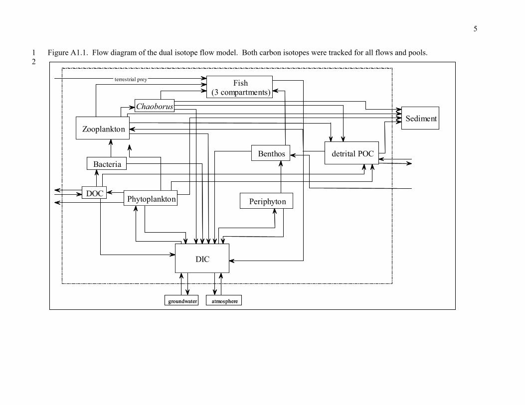
The dual-isotope flow (DIF) model calculates C flow for both 12C and 13C among 12 compartments within the lake and across the external boundaries of the ecosystem (Figure A1.1). The model is similar to a 6-compartment model presented in a prior paper (Cole et al. 2002), so we explain it only briefly here, highlighting the differences. The boundaries of the ecosystem are the bottom of the mixed layer, the atmosphere and the sediments. Two differential equations (one for mass balance dynamics of each C isotope) describe each of the 12 components of the model (DIC, DOC, pelagic bacteria, phytoplankton, detrital POC, zooplankton, Chaoborus, periphyton, benthic invertebrates, and three fish compartments representing different functional groups). Thus, there are 24 differential equations, one for the mass balance dynamics of 13C and one for the mass balance of total C in each of 12 compartments. The model was parameterized separately for each of the four experiments. Each of the 24 differential equations is a mass-balance equation (Cole et al. 2002). Many of the fluxes in each equation were directly measured. One flux for each carbon pool was estimated by difference. Eighteen parameters were estimated by constrained least squares using the Matlab Optimization Toolbox. The constraints were provided by literature values, our own measurements, or sensitivity analyses. These 18 parameters were input rate of POC; photosynthetic fractionation parameters for periphyton and phytoplankton; assimilation efficiencies of zooplankton and Chaoborus; respiration coefficients of benthos, zooplankton and Chaoborus; sedimentation coefficients of phytoplankton and zooplankton feces; flocculation and photodegradation coefficients of DOC; DOC release coefficient of phytoplankton; proportion of periphyton in benthos diets; selectivity coefficient of bacteria for DOC derived from phytoplankton; selectivity coefficient of zooplankton for phytoplankton; proportion of periphyton in benthos diets; relative contributions of zooplankton and Chaoborus to fish diets. The least squares estimates are the values of these parameters that minimize the sum of squared deviations between simulated and observed δ13C during the experiment. As a measure of goodness of fit, we present the residual standard deviation (standard deviation of the difference between simulated and observed δ13C values). This represents the average error of the model projections in the same units as δ13C (Appendix 4). The DIF model includes fish carbon fluxes computed by a fish bioenergetics model (Hanson et al. 1997). Bioenergetic parameters were taken from standard parameter tables for the fishes represented in the model (Hanson et al. 1997). For each fish compartment, the bioenergetics model was used to compute daily consumption of each prey item, respiration, and egestion. Growth and biomass dynamics were measured directly and interpolated to daily values input to the bioenergetics model. Fish functional groups were chosen to represent differences in body size and diet, and to include the most abundant fishes found in each experiment. In Paul Lake, Fish 1 is young-of-year largemouth bass, Fish 2 is juvenile largemouth bass, and Fish 3 is adult largemouth bass. Ontogenetic changes in diets of largemouth bass are reported in Carpenter and Kitchell (1993). In Peter Lake, Fish 1 is pumpkinseed (a sunfish that is primarily benthivorous), Fish 2 is stickleback (a small-bodied benthivore and planktivore), and Fish 3 is fathead minnow (a benthivorous cyprinid). In Tuesday Lake, Fish 1 is golden shiner (a primarily planktivorous cyprinid), Fish 2 is stickleback, and Fish 3 is fathead minnow.

3

In Tuesday Lake 2002, we did not simulate DI13C dynamics because good fits to observed δ13C of DIC could not be obtained. For that experiment, daily DI13C values were interpolated from measurements and used as inputs to the DIF model to solve the other 23 differential equations. DIC is a pH-dependent mixure of inorganic C species (CO2aq, HCO3 and CO3) and the reactions among these species fractionate 13C in different ways. Only the δ13C of the total DIC pool can be measured directly. The δ13C of the C species was calculated according to the equations in Zhang et al. (1995) and Mook et al. (1974). In nutrient-enriched Peter Lake in 2002, the very high pH and low CO2aq created conditions in which chemically-enhanced diffusion with the atomosphere occurred (Wanninkhof and Knox 1996). The uncertainty with isotope fractionation during chemically-enchanced diffusion made it difficult for us to accurately model all aspects of the DIC pool. Thus, the DIF for Peter Lake in 2002 uses actual measured DIC and its C-species isotopes as input data and does not model this compartment. A more complete treatment of the isotopic aspects of chemically enchanced diffusion in this experiment is presented by Bade (2004). The DIF model was solved in Matlab using a numerical method that accounted for the extremely rapid dynamics of DI13C in comparison with dynamics of 13C in other carbon pools. The 23 differential equations for compartments other than DI13C were integrated using the fourth-order fixed-interval Runge-Kutta method (Press et al. 1989). At each time step, DI13C was calculated using the analytic solution of the differential equation for DI13C. The analytical solution was derived by assuming that the other, more slowly-changing variables were constant over the short time step.

Programs for the model analysis and parameter bootstrapping were written by the authors using Matlab (versions 5.3 and 6.2).

LITERATURE CITED Bade, D.L. 2004. Ecosystem carbon cycles: whole-lake fluxes estimated with multiple isotopes. Ph.D. Thesis, University of Wisconsin, Madison, Wisconsin U.S.A. Carpenter, S.R. and J.F. Kitchell (eds.). 1993. The Trophic Cascade in Lakes. Cambridge University Press, Cambridge, England. Cole, J.J., S.R. Carpenter, J.F. Kitchell, and M.L. Pace. 2002. Pathways of organic C utilization in small lakes: Results from a whole-lake 13C addition and coupled model. Limnol. Oceanogr. 47: 1664-1675. Hanson, P.C., T.B. Johnson, D.E. Schindler, and J.F. Kitchell. 1997. Fish Bioenergetics 3.0. Sea Grant Technical Report. University of Wisconsin Sea Grant Institute, Madison, WI. Mook, W.G., J.C. Bommerson, and W.H. Stavernon. 1974. Carbon isotope fractionation between dissolved bicarbonate and gaseous carbon dioxide. Earth and Planetary Science Letters 22: 169-176.

4

Press, W.H., B.P. Flannery, S.A. Teukolsky and W.T. Vetterling. 1989. Numerical Recipes in C. Cambridge University Press, Cambridge, England. Wanninkhof, R. and M. Knox. 1996.Chemical enchancement of CO2 exchange in natural waters. Limnol.Oceanogr. 41: 689-697. Zhang, J., P.D. Quay, and D.O. Wilbur. 1995. Carbon isotope fractionation during gas-water exchange and dissolution of CO2.: Geochim. Cosmochim. Acta. 59:107-114.

1 2

Figure A1.1. Flow diagram of the dual isotope flow model. Both carbon isotopes were tracke

DIC

Bacteria

DOC Phytoplankton

atmospheregroundwater

Zooplankton

Periphyton

detrit

Chaoborus

Benthos

Fish(3 compartments)

terrestrial prey

DIC

Bacteria

DOC Phytoplankton

DIC

Bacteria

DOC Phytoplankton

atmospheregroundwater

Zooplankton

Periphyton

detrit

Chaoborus

Benthos

Fish(3 compartments)

terrestrial prey

5

d for all flows and pools.

al POC

Sediment

al POC

Sediment

6

APPENDIX 2. UNIVARIATE MODELS We used univariate statistical models to estimate sources supporting carbon pools and

food web constituents. The models are univariate because they only attempt to explain the response of a single variable (e.g. zooplankton) in contrast to other model approaches which are multivariate (Appendices 1 and 3). The models are statistical because they are based on fitting data from the C-13 manipulations using the equation: δ13Cxt = (1-w)[(1-m)(δ13CO2 (aq) – εp)t + m(δ13CO2 (aq) – εp)t-u] + w(-28). A schematic diagram of this model is presented in Figure A2.1. The left hand side of the equation represents time series of δ13C of POC, DOC, zooplankton, or Chaoborus (xt). The δ13C of these variables is modeled as a function of two sources - the δ13C of aqueous CO2 that varies during the manipulation and the δ13C of terrestrial C-3 plants that did not vary during the manipulation. The parameter w (0 ≤ w ≤ 1) estimates the relative contribution from these two sources. In addition, the contribution from aqueous CO2 is further divided into current production on day t and past production on day t - u where u is a time delay in days. The parameter m (0 ≤ m ≤ 1) estimates the relative contribution from current and past production. The distinction between current and past production accounts for the turnover of labeled carbon in the system. Comparisons showed that this distinction significantly improved the fit of the models to data (Pace et al. 2004). Aqueous carbon dioxide is the primary form of DI13C taken up by most phytoplankton and hence represents the carbon derived from primary production in the lake. The fractionation of 13C between CO2(aq) and HCO3 was calculated from direct measurements of DIC, DI13C, pH, and temperature using the equations of Mook et al. (1978) and Zhang et al. (1995). A daily time series of δ13CO2(aq) was established from measured values interpolated to daily values with a cubic spline. The model was evaluated for all the dates when δ13C of the response variable (POC, DOC zooplankton, or Chaoborus) was measured.

Unknown parameters for the univariate models are εp, w, m and u, where w, m, and u are as explained above and εp is photosynthetic fractionation. . The value of u that minimized variance was identified using a profile likelihood analysis (Burnham and Anderson 1998). Model parameters εp, w, and m were estimated using a nonlinear optimization routine in Matlab. Overall model fit was determined by least squares. Maximum likelihood analysis gave results equivalent to least squares for these models (Hilborn and Mangel 1997), but required estimating an additional parameter (variance). We only report the least squares results here. Goodness of fit was evaluated using mean residual standard deviation and the relationship between predicted and observed values. Parameter uncertainty was estimated by bootstrapping randomized data (Efron and Tibshirani 1993) and estimating parameters for 1000 iterations. The thousand estimates of each parameter were then used to calculate bootstrapped standard deviations. Bootstrapped parameter distributions for the models were approximately normally distributed, and parameter bias was only a few percent of the standard deviation (Efron and Tibshirani 1993).

The general model was modified for analysis of the 13C addition to Peter Lake in 2002.

In this case photosynthetic fractionation clearly varied and declined to low values with aqueous

7

CO2 drawdown promoted by nutrient addition. For this manipulation photosynthetic fractionation (εp) was modeled as a function of the concentration of CO2.

εp = ϕ [CO2] In this equation, the fitted parameter ϕ is negative, so εp becomes more negative as the concentration of CO2 increases. CO2 concentrations were measured or interpolated to match the date of sampling for modeled variables. ϕ was estimated using the same approach as described above for other parameters. Substituting equation 2 into equation 1 resulted in a model that provided a much better fit to the data for Peter Lake in 2002. For the analysis of DOC εp was fixed at the value derived for POC models excepting the Peter Lake 2002 manipulation. We assumed the autotrophic contribution to DOC is derived from the algae in the POC suggesting that photosynthetic fractionation from aqueous CO2 for these pools (POC and DOC) should be the same. In solutions that fit εp for the DOC data, fractionation was estimated near zero for the Paul and Peter 2001 additions. As an alternative, εp was fixed at the values derived for POC and parameters estimated using equation 1. Regardless of whether εp was fit or fixed the percent of allochthony for DOC was > 85% in the three manipulations that did not include nutrient addition. Here, we report results of models that used fixed values of εp.

Programs for the model analysis and parameter bootstrapping were written by the authors using Matlab (version 6.2).

LITERATURE CITED

Burnham, K.P. and D.R. Anderson. 1998. Model Selection and Inference: a Practical Information Theoretic Approach. Springer-Verlag, New York, New York. Efron, B and R.J. Tibshirani, 1993. An Introduction to the Bootstrap, Chapman & Hall, New York, New York. RHilborn, R. and M. Mangel. 1997. The Ecological Detective: Confronting Models with Data. Princeton University Press, Princeton, New Jersey. Mook, W.G., J.C Bimmerson, and W.H. Staverman. 1974. Carbon isotope fractionation between dissolved bicarbonate and gaseous carbon dioxide. Earth and Planetary Science Letters 22: 169-176. Pace, M.L., J.J. Cole, S.R. Carpenter, J.F. Kitchell, J.R. Hodgson, M. Van de Bogert, D.L. Bade, E.S. Kritzberg, and D. Bastviken. 2004. Whole-lake carbon-13 additions reveal terrestrial support of aquatic food webs. Nature 427: 240-243. Zhang, J., P.D. Quay, and D.O. Wilbur. 1995. Carbon isotope fractionation during gas-water exchange and dissolution of CO2.: Geochim. Cosmochim. Acta. 59:107-114.

8

Figure A2.1. Schematic diagram of the univariate models. Symbols are defined in the text.

δ13C xtime = t

x = POC, DOC,zooplankton, orChaoborus

δ13CO2 – εtime = t

(current production)

δ13C = -28(terrestrial)

δ13CO2 – εtime = t - u

(past production)

m

w

9

APPENDIX 3 MULTIVARIATE AUTOREGRESSION MODELS Multivariate autoregressions (Ives et al. 2003) were used to estimate autochthony and allochthony. The general form of the transition equation was

αt = B αt-1 + C Ut + ωt

In the transition equation, α is a vector of δ13C in components of the food web at a specified time. Elements of the transition matrix B describe the interactions among food web components. U is a matrix of covariates, and C is a matrix of parameters for the effects of the covariates. The errors ω are assumed to follow a multivariate normal distribution with mean 0 and covariance matrix Q.

We accounted for sampling errors in observing δ13C. Although analytical errors in measuring δ13C are small, it may be important to account for variation among replicate samples of consumers. We accounted for observation errors using an equation

yt = αt + υt

Here y is vector of observed δ13C at a specified time and the observation errors υ were assumed to follow a multivariate normal distribution with mean 0 and covariance matrix H. Given data for y and U and estimates of the observation covariance matrix H, a Kalman Filter was used to compute maximum likelihood estimates of B, C and Q (Harvey 1989). Using the elements of B and C, we estimated autochthony and allochthony (see below). We computed standard deviations of the elements of B and C, and of autochthony and allochthony, by parametric bootstrapping as recommended by Ives et al. (2003). To understand the calculation of autochthony and allochthony, it is necessary to examine the specific transition equations that were analyzed. For each lake-year, we analyzed two transition equations, one for the littoral data and one for the pelagic data. In the benthic transition equation (Figure A3.1),

=

bp

α

−

−=

b

p

mm

B10

01

−−

=bbb

ppp

wggwgg

Cεε

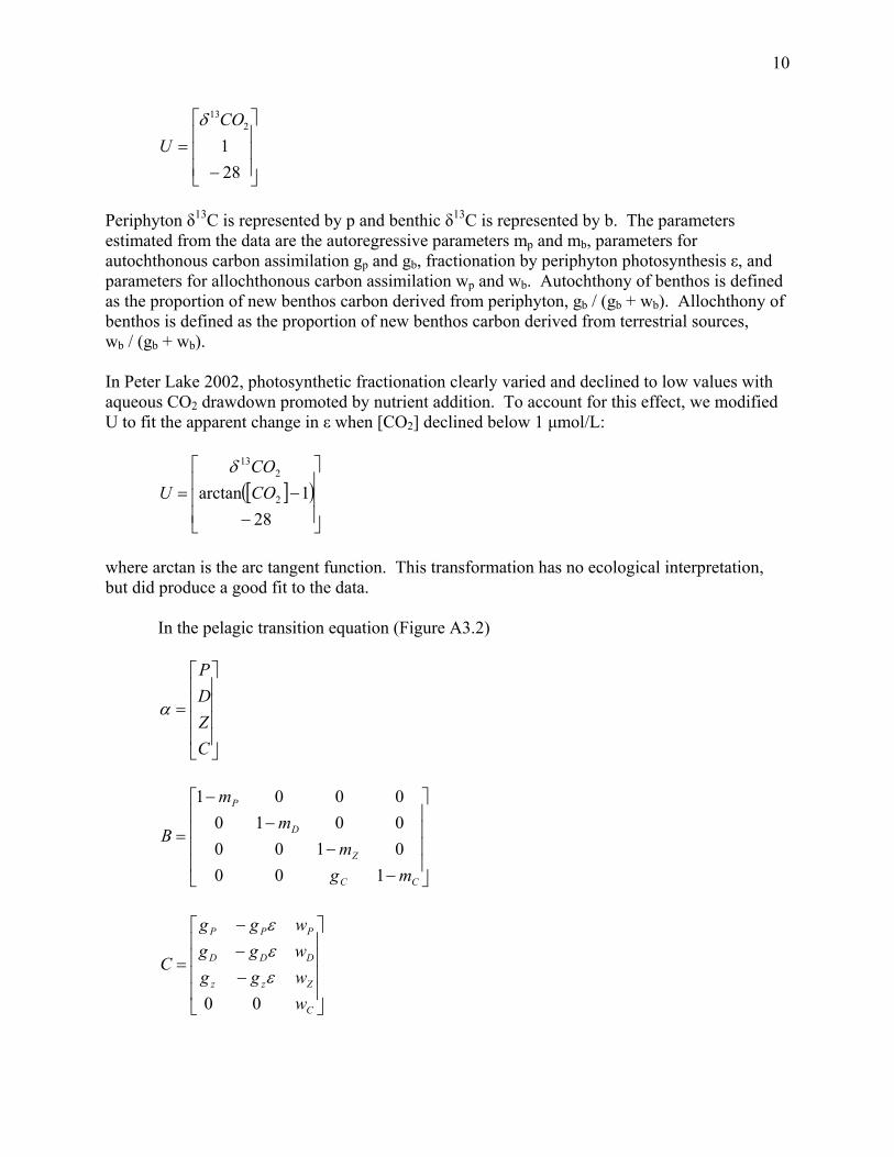
10

−=

281

213CO

Uδ

Periphyton δ13C is represented by p and benthic δ13C is represented by b. The parameters estimated from the data are the autoregressive parameters mp and mb, parameters for autochthonous carbon assimilation gp and gb, fractionation by periphyton photosynthesis ε, and parameters for allochthonous carbon assimilation wp and wb. Autochthony of benthos is defined as the proportion of new benthos carbon derived from periphyton, gb / (gb + wb). Allochthony of benthos is defined as the proportion of new benthos carbon derived from terrestrial sources, wb / (gb + wb). In Peter Lake 2002, photosynthetic fractionation clearly varied and declined to low values with aqueous CO2 drawdown promoted by nutrient addition. To account for this effect, we modified U to fit the apparent change in ε when [CO2] declined below 1 µmol/L:

[ ]( )

−−=

281arctan 2

213

COCO

Uδ

where arctan is the arc tangent function. This transformation has no ecological interpretation, but did produce a good fit to the data. In the pelagic transition equation (Figure A3.2)

=

CZDP

α

−−

−−

=

CC

Z

D

P

mgm

mm

B

100010000100001

−−−

=

C

Zzz

DDD

PPP

wwggwggwgg

C

00εεε

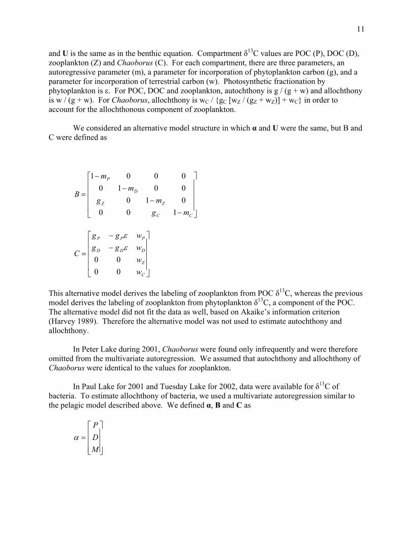
11

and U is the same as in the benthic equation. Compartment δ13C values are POC (P), DOC (D), zooplankton (Z) and Chaoborus (C). For each compartment, there are three parameters, an autoregressive parameter (m), a parameter for incorporation of phytoplankton carbon (g), and a parameter for incorporation of terrestrial carbon (w). Photosynthetic fractionation by phytoplankton is ε. For POC, DOC and zooplankton, autochthony is g / (g + w) and allochthony is w / (g + w). For Chaoborus, allochthony is wC / {gC [wZ / (gZ + wZ)] + wC} in order to account for the allochthonous component of zooplankton. We considered an alternative model structure in which α and U were the same, but B and C were defined as

−−

−−

=

CC

ZZ

D

P

mgmg

mm

B

10001000100001

−−

=

C

Z

DDD

PPP

wwwggwgg

C

0000

εε

This alternative model derives the labeling of zooplankton from POC δ13C, whereas the previous model derives the labeling of zooplankton from phytoplankton δ13C, a component of the POC. The alternative model did not fit the data as well, based on Akaike’s information criterion (Harvey 1989). Therefore the alternative model was not used to estimate autochthony and allochthony. In Peter Lake during 2001, Chaoborus were found only infrequently and were therefore omitted from the multivariate autoregression. We assumed that autochthony and allochthony of Chaoborus were identical to the values for zooplankton. In Paul Lake for 2001 and Tuesday Lake for 2002, data were available for δ13C of bacteria. To estimate allochthony of bacteria, we used a multivariate autoregression similar to the pelagic model described above. We defined α, B and C as

=

MDP

α

12

−−

−=

M

D

P

mm

mB

100010001

=

MMM

DDD

PPP

wggwggwgg

Cεεε

Symbols are identical to those for the pelagic model, except that M represents bacterial δ13C. Autochthony of bacteria is gM / (gM + wM) and allochthony is wM / (gM + wM). We also considered an alternative model in which labeling of bacteria was linked to bulk DOC, instead of to carbon released by phytoplankton. For this alternative model, B and C are defined as

−−

−=

MM

D

P

mgm

mB

10010001

=

M

DDD

PPP

wwggwgg

C00

εε

This alternative model did not fit as well, according to Akaike’s information criterion (Harvey 1989). Therefore it was not used to compute autochthony and allochthony.

Programs for the model analysis and parameter bootstrapping were written by the authors using Matlab (version 5.3).

LITERATURE CITED Harvey, A.C. 1989. Forecasting, Structural Time Series Models, and the Kalman Filter. Cambridge University Press, Cambridge, England. Ives, A.R., B. Dennis, K.L. Cottingham and S.R. Carpenter. 2003. Estimating community stability and ecological interactions from time-series data. Ecological Monographs 73: 301-330.

13

Figure A3.1. Schematic diagram of the MAR model used to estimate allochthonous and autochthonous carbon flow to benthos. Benthos are linked to periphyton through consumption of current production. Measurements of periphyton δ13C could have included small amounts of terrestrial detritus as well as in-lake primary production, represented by the arrow from terrestrial carbon to periphyton. Symbols are defined in the text.

δ13Cperiphyton

time = t

δ13Cbenthostime = t

δ13CO2 – εtime = t

(current production)


δ13Cperiphytontime = t -1

δ13Cbenthos

time = t -1

1 - mp

1 - mb

gb

wb

gp

wp

14

Figure A3.2. Schematic diagram of the MAR model used to estimate allochthonous and autochthonous carbon flow to POC, DOC, zooplankton and Chaoborus. POC, DOC and zooplankton are linked to phytoplankton through current production, whereas Chaoborus carbon derives from zooplankton. δ13CO2 – ε

time = t(current production)


δ13C POCtime = t

δ13C DOCtime = t δ13C

zooplanktontime = t

δ13CChaoborus

time = t

δ13C POCtime = t

δ13C DOCtime = t δ13C

zooplanktontime = t

δ13CChaoborus

time = t

gC

δ13C POCtime = t - 1

δ13C DOCtime = t - 1

δ13Czooplanktontime = t - 1

δ13CChaoborustime = t - 1

gZ

gP

gD

1 - mP

1 - mD

1 - mZ

1 - mC

wP

wD wZ

wC

15

APPENDIX 4 GOODNESS-OF-FIT OF THE MODELS 1 2 3 4 5 6 7 8 9

10 11 12 13

Standard deviations of residuals for each carbon pool were similar for the three models (Table A4.1). Standard deviations of residuals were substantially smaller than the ranges of δ13C caused by the tracer additions. Table A4.1. Ranges (per mil) and standard deviations of residuals (per mil) for δ13C of each carbon pool. For each experiment, we present the range of observed δ13C and the residual standard deviation from predictions of univariate (Uni), multivariate autoregressive (MAR), and dual-isotope flow (DIF) models. Residual standard deviations were not available (n/a) for carbon pools that were not predicted by a model. In Paul Lake, Fish 1 is young-of-year largemouth bass, Fish 2 is juvenile largemouth bass, and Fish 3 is adult largemouth bass. In Peter Lake, Fish 1 is pumpkinseed, Fish 2 is stickleback, and Fish 3 is fathead minnow. In Tuesday Lake, Fish 1 is golden shiner, Fish 2 is stickleback, and Fish 3 is fathead minnow.

16

1 2

Paul Lake, 2001 Peter Lake, 2001 Peter Lake, 2002 Tuesday Lake, 2002 Compartment Range Uni MAR DIF Range Uni MAR DIF Range Uni MAR DIF Range Uni MAR DIFDIC 39.0 n/a n/a 0.9 37.4 n/a n/a 0.6 41.0 n/a n/a n/a 42.0 n/a n/a 3.4DOC 5.0 1.0 0.2 0.2 3.0 0.6 0.2 0.2 9.5 1.9 0.05 0.4 1.9 0.4 0.2 0.1POC 23.1 1.6 0.5 0.7 16.6 1.5 0.01 0.4 42.8 5.8 0.03 0.7 21.1 2.8 0.2 1.2Bacteria 14.1 n/a 1.9 0.5 7.7 n/a n/a 0.7 22.3 n/a n/a 1.6 10.2 n/a 1.3 0.4Zooplankton 29.4 2.2 0.4 0.5 18.6 0.8 1.0 0.7 37.9 3.3 0.5 1.8 11.2 1.6 0.4 1.7Chaoborus 23.3 4.5 0.2 0.9 8.5 n/a n/a 4.2 28.4 5.3 0.3 1.9 13.8 2.0 0.7 0.8Periphyton 30.7 n/a 2.3 2.1 30.0 n/a 2.7 1.5 44.7 n/a 1.6 2.8 50.9 n/a 0.4 3.0Benthos 11.6 n/a 2.2 0.8 n/a n/a n/a n/a 23.4 n/a 1.4 1.0 18.7 n/a 0.3 0.7Fish 1 18.7 n/a n/a 0.8 6.8 n/a n/a 0.4 16.1 n/a n/a 1.0 5.5 n/a n/a 0.3Fish 2 10.0 n/a n/a 0.9 11.0 n/a n/a 0.6 16.4 n/a n/a 0.9 12.2 n/a n/a 0.8Fish 3 0.7 n/a n/a 0.5 11.4 n/a n/a 0.6 16.4 n/a n/a 0.9 9.9 n/a n/a 0.3 3

4 5 6

ecosystem subsidies: terrestrial support of aquatic food webs from

Documents