ecosystem considerations 2017 · mayumi arimitsu, sonia batten, jennifer boldt, nick bond, jennifer...

Ecosystem Considerations 2017

Status of theGulf of Alaska Marine Ecosystem

Edited by:Stephani Zador1 and Ellen Yasumiishi2

1Resource Ecology and Fisheries Management Division, Alaska Fisheries Science Center,National Marine Fisheries Service, NOAA

2Auke Bay Laboratories, Alaska Fisheries Science Center,National Marine Fisheries Service, NOAA

With contributions from:

Mayumi Arimitsu, Sonia Batten, Jennifer Boldt, Nick Bond, Jennifer Cedarleaf, Kristin Cieciel,Seth Danielson, Annette Dougherty, Sherri Dressel, AnneMarie Eich, Nissa Ferm, Emily Fergusson,Ben Fissel, Shannon Fitzgerald, Christine Gabriele, Sarah Gaichas, Andrew Gray, Chuck Guthrie,Dana Hanselman, Coleen Harpold, Bradley Harris, Scott Hatch, Kyle Hebert, Jerry Hoff, SteveKasperski, Arthur Kettle, David Kimmel, Carol Ladd, Ned Laman, Jesse Lamb, Anna Lavoie,Jean Lee, Daniel Lew, Steve Lewis, Jennifer Mondragon, John Moran, Jamal Moss, Franz Mueter,Jim Murphy, Janet Neilson, Joseph Orsi, Wayne Palsson, Melanie Paquin, Heidi Pearson, JohnPiatt, Alexei Pinchuk, Steven Porter, Heather Renner, Patrick Ressler, Lauren Rogers, Nora Rojek,Chris Rooper, Joshua Russell, Kalei Shotwell, Kim Sparks, William Stockhausen, Janice Straley,Wes Strasburger, Andy Szaba, Marysia Szymkowiak, Louise Taylor-Thomas, Scott Vulstek, JordanWatson, Andy Whitehouse, Matthew Wilson, Sarah Wise, Carrie Worton, Ellen Yasumiishi, andStephani Zador

Reviewed by:The Gulf of Alaska Groundfish Plan Team

November 13, 2017North Pacific Fishery Management Council

605 W. 4th Avenue, Suite 306 Anchorage, AK 99301

2

Western Gulf of Alaska 2017 Report Card

� The Gulf of Alaska in 2017 remained characterized by warm conditions although conditions havemoderated since the extreme heat wave of 2014–2016. The PDO remains in a positive patternbut with lower amplitude.

� The freshwater runoff into the GOA appears to have been greater than normal duringthe fall of 2016 and somewhat less than normal in summer 2017, with implications for thebaroclinic component of the Alaska Coastal Current.

� Mesozooplankton biomass measured by the continuous plankton recorder has often shown alargely biennial trend, however biomass remained greater than average in 2014 – 2016. Biomasstrends can be influenced by ecosystem conditions and mean size of the community. This suggeststhat prey availability for planktivorous fish, seabirds, and mammals has been variable recently. Thebiennial patterns suggests a possible link with biennially varying planktivorous pink salmonabundance which have shown lower than expected marine survival for the 2015 and 2016 outmigrationyear classes.

� Copepod community size remained small for the fourth consecutive year. The prevalenceof small copepods fits predictions of warm conditions favoring small copepods. This suggests thatplanktivorous predators may have had to work harder to fill nutritional needs from thenumerous, but small, prey items.

� Bottom trawl survey biomass of motile epifauna was below its long-term mean for the firsttime since 2001. The increase from 1987 to 2001 was driven by hermit crabs and brittle stars, whichcontinue to dominate the biomass. Octopus catches, which were record high in 2015, declined to a lownot seen since 1990.

� Trends in capelin as sampled by seabirds and groundfish have indicated that capelin were abundantfrom 2008 to 2013, but declined in during the warm years of 2015–2016. Their apparentabundance coincided with the period of cold water temperatures in the Gulf of Alaska.Preliminary reports suggest that predators were again foraging on capelin in 2017.

� Fish apex predator biomass during 2017 bottom trawl surveys was at its lowest level inthe 30 year time series, and the recent 5 year mean is below the long-term average. The trendis driven primarily by Pacific cod and arrowtooth flounder which were both at the lowestabundance in the survey time series. Pacific halibut and arrowtooth flounder have shown a generaldecline since their peak survey biomasses in 2003. Pacific cod has continued to decline from apeak survey biomass in 2009.

� Black-legged kittiwakes had moderate reproductive success in 2017 at the Semedi Islands,in contrast to the complete failure in 2015 for kittiwakes as well as other seabird species. Their repro-ductive success is typically variable, presumably reflecting foraging conditions prior to the breedingseason, during, or both. In general, fish-eating seabirds had less successful reproduction in 2017 thanmixed fish and plankton-eating seabird species.

� Modelled estimates of western Gulf of Alaska Steller sea lion non-pups counts were ap-proaching the long-term in 2016, suggesting conditions had been favorable for sea lions in thisarea. However, preliminary estimates show a decline in the number of pups from 2015 to 2017 anddeclines in the number of non-pups in the Cook Inlet, Kodiak, and Semidi area.

� Human populations in the small (<1500 people) fishing communities in the western Gulf of Alaskahave remained stable as a whole since 2000.

1

-2

1

4

* Pacific Decadal Oscillation (Winter)

10000

25000

40000

Fresh Water Input

-1

0

1* Mesozooplankton Biomass

-0.1

0.1

0.3

* Copepod Community Size

0

10000

20000

* Motile Epifauna Biomass

-3

0

3Capelin DFA Index

1000

3000

5000

* Apex Fish Biomass

-0.1

0.5

1.1

* Black-legged kittiwake Reproductive Success

10000

40000

70000

* Steller Sea Lion Non-pups

11000

15000

19000 * Human Population (Small Communities)

1970 1980 1990 2000 2010 2017

2013-2017 Mean 2013-2017 Trend

1 s.d. above mean

1 s.d. below mean

within 1 s.d. of mean

fewer than 2 data points

increase by 1 s.d. over time window

decrease by 1 s.d. over time window

change <1 s.d. over window


Figure 1: Western Gulf of Alaska ecosystem assessment indicators; see text for descriptions. * indicatestime series updated in 2017.

2

Eastern Gulf of Alaska 2017 Report Card

� The Gulf of Alaska in 2017 remained characterized by warm conditions although conditions havemoderated since the extreme heat wave of 2014–2016. The neutral El Nino of last winter haslessened, and La Nina conditions are slightly more favored that neutral for next winter.

� The sub-arctic front was farther south than usual, which was consistent with surface currents.Strong winter winds from the north impelled the PAPA trajectory index to its most southerly latitudesince the late 1930s. This represented a substantial change from the northerly surface current patternduring the previous three winters.

� Total zooplankton density in Icy Strait increased in 2016 relative to the previous threeyears but remained lower than the peak values in 2006–2009. Zooplankton were numerically dom-inated by gastropods and small copepods, while large copepod and euphausiid densities remainedbelow average.

� Also in Icy Strait, the increase in large and decrease in small copepod abundances in 2016relative to the previous year resulted in an increase in copepod community size. However, the lowabundances of all copepods does not indicate substantially improved foraging conditions forplanktivorous predators.

� Bottom trawl survey biomass of motile epifauna is typically dominated by brittle stars anda group composed of sea urchins, sand dollars and sea cucumbers. Record catches of hermitcrabs influenced the peak biomass estimate in 2013. Catches of many of the more dominant membersof this foraging guild were low in 2015. Brittle stars and miscellaneous crabs were the most abundantin 2017.

� A decrease in estimated total mature herring biomass in southeastern Alaska has beenobserved since the peak in 2011. Modeling indicates that the declines in biomass may be relatedto lower survival.

� Bottom-trawl survey fish apex predator biomass is currently below its 30-year mean, followinga peak in 2015. The trend is driven primarily by arrowtooth flounder which caught in greatnumbers in 2015. Pacific halibut and sablefish, the next most abundant species in this foraging guildhave shown variable but generally stable trends in recent surveys. Pacific cod were at their lowestabundance in the time series in 2017, but had been at their highest relative abundance in 2015.

� Growth rates of piscivorous rhinoceros auklet chicks were anomalously low in 2015 and2016, suggesting that the adult birds were not able to find sufficient prey to support successful chickgrowth. This is in contrast to 2012 and 2013, when chick growth rates were above the long termaverage.

� Modelled estimates of eastern Gulf of Alaska Steller sea lion non-pups counts are above the longterm mean through 2015. However, preliminary estimates suggest that non-pup counts declined12% in 2017 relative to 2015. This unusual recent decline in a long-increasing stock may indicateadverse responses to the marine heat wave of recent years.

� Human populations in the small (<1500 people) fishing communities in the eastern Gulf of Alaskahave remained stable in recent years following a gradual decline since peak population counts inthe mid-1990s.

3

-2

1

4

* Multivariate ENSO Index (MEI DecJan)

-0.1

0.1

0.3

Oceanography Index TBD

0

2000

4000

* Zooplankton Density Icy Strait (#/m3)

0.1

0.3

0.5

* Copepod Community Size

0

400

800* Motile Epifauna Biomass

0

150000

300000

* SE Alaska Herring Mature Biomass (tons)

100

250

400

* Apex Fish Biomass

6

10

14

Rhinoceros Auklet Chick Growth

0

15000

30000

* Steller Sea Lion Non-pups

8000

9500

11000* Human Population (Small Communities)

1970 1980 1990 2000 2010 2017

2013-2017 Mean 2013-2017 Trend

1 s.d. above mean

1 s.d. below mean







Figure 2: Eastern Gulf of Alaska ecosystem assessment indicators; see text for descriptions. Onepotential indicator is yet to be determined (TBD). * indicates time series updated in 2017.

4

Executive Summary of Recent Trendsin the Gulf of Alaska

This section contains links to most new and updated information contained in this report. Thelinks are organized within three sections: Physical and Environmental Trends, Ecosystem Trends,and Fishing and Human Dimensions Trends.

Physical and Environmental Trends

North Pacific

� The North Pacific atmosphere-ocean climate system was in a more moderate state during 2016–2017than during the previous two years (p. 61).

� In particular, the warm sea surface temperature anomalies associated with the extreme marine heatwave of 2014–2016 moderated (p. 56).

� A weak La Nina developed during winter 2016–2017 along with a weaker than normal Aleutian Low(p. 61).

� The Pacific Decadal Oscillation remains positive but with lower amplitude than in recent past years(p. 61).

� The winter of 2016–2017 included a large positive value for the North Pacific Index (NPI). While thissign of the NPI represents a typical atmospheric response to La Nina, its magnitude was dispropor-tionately large considering the weak amplitude of La Nina in late 2016 (p. 61).

� The North Pacific Gyre Oscillation (NPGO) mostly declined from a small positive value in early 2016to a small negative value in early 2017, implying that flows in the Alaska Current portion of theSubarctic Gyre and the California Current weakened slightly (p. 61).

� Climate models used for seasonal weather predictions indicate neutral to weak La Nina conditions forthe winter of 2017–2018 (p. 63).

� A continuation of warm sea surface temperatures across most of the North Pacific is predicted through

the end of the year. The magnitude of the anomalies is projected to be greatest in the western Bering

Sea, followed by slight cooling in the eastern Bering Sea, Gulf of Alaska, and nearshore waters of the

Pacific Northwest during spring 2018 (p. 63).

Gulf of Alaska

� The weather of the coastal GOA was generally warmer than normal during the past year with theexception of winter 2016–2017, during which air temperatures were near normal (p. 56).

5

� The coastal wind anomalies were upwelling favorable during the winter (p. 56).

� The freshwater runoff into the GOA appears to have been greater than normal during the fall of 2016and somewhat less than normal in summer 2017, with implications for the baroclinic component ofthe Alaska Coastal Current (p. 56).

� A prominent eddy formed near Yakutat in January 2016, leading to eddy kinetic energy levels in thenorthern Gulf of Alaska during spring 2016 were the highest recorded. Thus, phytoplankton biomasswas likely not confined to the shelf and cross-shelf transport of heat, salinity and nutrients was likelystrong (p. 65).

� Relatively weak eddy kinetic energy was observed in both the northern Gulf of Alaska and south ofKodiak during spring 2017 (p. 65).

� The sub-arctic front was farther south than usual, which is consistent with the surface currents shownin the Papa Trajectory Index (p. 67).

� The PAPA Trajectory Index recorded its southernmost latitude since the late 1930s. Strong winterwinds pushed the drifter track to the south east, in contrast to the north easterly direction of the pastthree years (p. 67).

� Water temperatures during the 2017 bottom trawl survey were slightly cooler compared to 2015 butstill among the warmer years in the record. The 2017 GOA thermal profile shared characteristics ofthe other warm survey years (i.e., 2003, 2005, and 2015) and contrasts with the cooler survey years(e.g., 2007–2013). The warmest water did not penetrate as deeply into the upper 100 m in 2017 (p.70).

� Freshwater temperatures in Auke Creek were above average during 2016 and average during during2017 relative to the long term 1980–2017 average (p. 75).

� Auke Creek water depths were higher than average during March-April and August, and lower thanaverage May–July during 2017 (p. 75).

� Sea surface temperatures in Icy Strait were ∼0.5oC below the 20-year time series average (p. 92).

� Sea temperatures on the Eastern Gulf of Alaska shelf at the surface and at the average mixed layerdepth were cooler in 2017 than 2016 (p. 90).

Ecosystem Trends

� In the Alaskan Shelf region sampled by the continuous plankton recorder, diatom abundance anomalieswere very low in 2016, representing a substantial decline relative to the previous six years (p. 80).

� In the same region, copepod community size anomalies remained negative for the fourth year (2013–2016), while mesozooplankton biomass anomalies were positive (and highest) for the third consecutiveyear (p. 80).

� Based on rapid zooplankton assessments in spring and summer 2017 in the western Gulf of Alaska,large copepod abundances in 2017 appeared to be higher than 2015 and similar in magnitude to thelong-term estimates from Line 8 (p. 83).

� In the same surveys, small copepods were abundant throughout the sampling area in spring, and theirabundances increased during summer. 2017 values were similar to the long-term estimates (p. 83).

� There were two types of surveys that sampled euphuasiids in the western Gulf of Alaska during 2017.There was a decline in acoustically-determined euphausiid abundance during summer 2017 relativeto the previous survey in 2015, to a low value similar to 2003 (p. 87). In the rapid zooplanktonassessment, euphausiid abundances appeared to be much higher than historical estimates in springand much higher than 2015 in particular (p. 83).

6

� Comprehensive zooplankton analysis from the eastern Gulf of Alaska showed patchy distribution ofspecies during 2017 with 40% of the total biomass to Cnidarian (nearshore) and Tunicates (basin) (p.94).

� Zooplankton density in Icy Strait increased in 2016 relative to the previous three years but remainedlower than the peak values in 2006–2009. Zooplankton were numerically dominated by gastropodsand small copepods, while large copepod and euphausiid densities remained below average (p. 92).

� The bottom trawl survey shows very few trends in total jellyfish abundance across time, with most ofthe trends being consistent within regions (p. 101).

� Diversity and abundance of jellyfish community during the EGOA summer survey increased in 2017with a shift away from single-species dominate (Phacellophora) observed in 2016 (p. 101).

� ADF&G survey biomass of Pacific herring in southeast Alaska in 2016 continued the decline from thepeak in 2011. All but Sitka herring stocks were at the lowest level in the time series, 1980–2016 (p.127).

� Neither sand lance nor capelin were prevalent during 2013–2016 in forage fish sampled by seabirds atMiddleton Island. Instead, mytophids and salmon increased in frequency (p. 112).

� The 2017 summer young-of-year sablefish-targeted trawl survey caught very few sablefish (2017 yearclass) within the survey grid, but caught more opportunistically near Kayak Island. Sebastes spp.catches in 2017 were similar to 2016.

� The 2017 summer eastern Gulf of Alaska shelf surface trawl survey biomass estimates for juvenile werelow for squid, juvenile Pacific cod, juvenile walleye pollock, and juvenile rockfish, but high for juvenilearrowtooth flounder. Biomass estimates for juvenile salmon were lowest on record for juvenile Chinooksalmon and juvenile coho salmon, low for juvenile pink and sockeye salmon, and moderate for juvenilechum salmon (p. 124, 116, and 120)

� At the Auke Creek weir, the marine survival of wild coho salmon for the 2016 smolt year was lowestthe on record for age-1 for the 38 year time series (p. 133).

� Marine survival of wild pink salmon for the 2016 smolt year was below average but above average overthe last 5 years (p. 131).

� Fish CPUE in Icy Strait was the lowest on record for juvenile salmon, low for capelin, larval pollock,adult pollock, moderate for immature Chinook salmon, and high for adult chum salmon and herringin 2017 relative to 1997-2016 (p. 130).

� Above average recruitment of sablefish to age-2 in 2018 (69 million) is expected based on warm latesummer sea temperatures and high chlorophyll a values in Icy Strait waters of northern southeastAlaska during 2016 (p. 144).

� In 2017 groundfish condition was below average for all species except Pacific cod. Northern rockfishand arrowtooth flounder had the lowest condition on record, and Pacific Ocean perch and southernrock sole were the second lowest on record (p. 135).

� In the Gulf of Alaska, there continues to be no significant trends in the distribution of rockfish withdepth, temperature and position. The stability of the distribution indicates that each of the speciesoccupy a fairly specific depth distribution. As temperatures rise and fall around the mean, the depthdistribution does not change, indicating that the rockfish are not changing their habitat or distributionto maintain a constant temperature (p. 147).

� Arrowtooth flounder, flathead sole, and other flatfish continue to dominate the catches in the ADF&Gtrawl survey, but not to the same degree as seen in previous surveys. A sharp decrease in overallbiomass is apparent from 2007 to 2016 from the years of record high catches occurring from 2002 to2005 (p. 139).

7

� Below average anomaly values for arrowtooth flounder and flathead sole were recorded again in 2016for both inshore and offshore areas; along with walleye pollock and Pacific cod. Pacific halibut andskates were above in both areas, while Tanner crab was above average only in the offshore area (p.139).

� Total CPUE in both the eastern and western GOA bottom trawl survery decreased from recent highvalues to their lowest (west) and second lowest (east) value in 2017. Species that showed the largestabsolute declines in biomass since 2013 included walleye pollock, Pacific cod, arrowtooth flounder andnorthern rockfish in the western GOA; and arrowtooth flounder, shortraker rockfish, Pacific cod andspiny dogfish in the eastern GOA (p. 158).

� Species richness and diversity are generally higher in the eastern Gulf of Alaska than in the westernGulf. Both richness and diversity tend to be highest along the shelf break and slope, with richnesspeaking at or just below the shelf break (200-300m), and diversity peaking deeper on the slope as wellas in shallow water. Diversity in the eastern Gulf has been declining since 2007 (p. 160).

� Few “mushy” halibut were reported during the 2017 fishing season relative to the previous few years,possibly indicating improved foraging conditions for halibut (p. 163).

� Ichthyophonus, a non-specific fungus-like protozoan fish parasite, has caused epizootic events amongeconomically important fish stocks including herring and salmon. Current research has found noindication of high intensity infections or clinically diseased individuals, supporting the hypothesis thatunder typical conditions, Ichthyophonus can occur at high infection prevalence with concomitant lowinfection intensities (p. 163).

� Several fish-eating seabirds had unusually low reproductive success in 2017. Common murres, whichshowed rare widespread reproductive failure in 2015–2016, generally had better colony attendance andfledging rates in 2017 but still the number of birds breeding was low. Black-legged kittiwakes andstorm-petrels (which consume a mix of fish and invertebrates) showed fledging rates within 1 SD ofthe mean, as did planktivorous auklets ( p. 152).

� Humpback whale calving and juvenile return rates in Glacier Bay and Icy Strait have declined sub-stantially in recent years. An anomalously low crude birth rate is expected for 2017. These changesin calving and juvenile return rates may be related to recent changes in whale prey availability and/orquality, which may in turn be negatively affecting maternal body condition and therefore reproductivesuccess and/or overall juvenile survival (p. 154).

� Observations of humpback whales throughout Prince William Sound and southeast Alaska suggestthat there is a long-term trend in humpback whales in Gulf of Alaska that may be related to prey. Ifprey is limiting and humpback whale populations have fully recovered to carrying capacity, there ispotential for top-down forcing on forage species and competition with fish, other marine mammals,and seabirds (p. 156).

Fishing and Human Dimensions Trends

� Discard rates of groundfish in the Gulf of Alaska increased from <10% in 2015 to >11% in 2016 forthe fixed gear sector; remained low, fluctuating between 1-3%, for the pollock trawl sector since 1998;and generally declined over the last ten years to a low of 8% in 2015 and 2016 for the non-pollocktrawl sector (p. 165).

� Non-target species catch of Schyphozoan jellies, primarily captured in the pollock fishery, was highestin 2016 relative to 2011–2016. Sea stars comprise 90% of the catch of assorted invertebrates. They areprimarily captured in the Pacific cod and halibut fisheries. Catch of structural epifauna has trendedupward since 2012. These are mostly sea anemones caught in the flatfish, Pacific cod, and sablefishfisheries (p. 169).

8

� Stock Composition of Chinook salmon bycatch in the Gulf of Alaska trawl fisheries has been relativelystable from 2012–2015. British Columbia stocks dominate the bycatch, and West Coast U.S. stockseither similar to British Columbia stocks, or less, in most years. The 2015 stock composition includedChinook salmon from British Columbia (51%), West Coast U.S. (32%), coastal southeast Alaska (14%),and northwest Gulf of Alaska (3%) (p. 170).

� Estimated numbers of seabird caught incidentally in the groundfish fisheries decreased from 876 to626 from 2015 to 2016 primarily due to a reduction in bycatch by 43% for black-footed albatross, 48%for gull, 100% for cormorant, and 43% for unidentified birds. No cormorant, other alcid, auklets, orunidentified albatross were caught (p. 173).

� At present, no GOA groundfish stock or stock complex is subjected to overfishing, and no GOAgroundfish stock or stock complex is considered to be overfished or to be approaching an overfishedcondition (p. 177).

� Landings (pounds) to characterize commercial seafood production decreased from 2015 to 2016 pri-marily due to a reduction in salmonid landings, then apex predators, and motile epifauna. Increasesin landing occurred in pelagic and benthic foragers (p. 182).

� Halibut and salmon (94% sockeye) subsistence harvest trends increased slightly from 2013 to 2014.However, over a longer period, 2005 to 2014, trends show roughly a 30% decline in halibut harvestand 40% increase in salmon harvest for subsistence (p. 183).

� Economic values of 5 functional groups (apex predators, benthic foragers, motile epifauna, pelagicforagers, and salmonids) show a decline in real ex-vessel value overall in all groups, a decline in thereal first-wholesale value in all groups except benthic foragers and motile epifauna, and an increase ofroughly 20% in the ratio of first-wholesale to total catch unit value for groups combined from 2015 to2016 (p. 187).

� Saltwater recreational fishing participation included almost 1 million days fished and an increase fromapproximately 375,000 to 390,000 saltwater anglers from 2014 to 2015 (p. 191).

� The trend in unemployment as an indicator of community viability increased in 2016 relative to 2015and was slightly higher 4.8% than the national unemployment rates of 4.6% in 2016 (p. 194).

� Trends in human populations from 2010 to 2016 indicate a 4.17% increase for Alaska, 2.98% increase forGulf of Alaska communities including Anchorage, and a 3.98% increase for Gulf of Alaska communitiesnot including Anchorage (p. 196).

� School enrollment has remained fairly stable recently, showing a slight decrease for larger schoolswith 500-4,500 students. Smaller schools had more variable enrollment year-to-year and an overalldownward trend. As of 2017, 27 schools have enrollment under 30 students, and 12 schools haveenrollments under 15 students, and 7 schools were closed (p. 199).

9

Contents

*GOA Report Card . . . . . . . . . . . . . . . . . . . . . . . . . . . . . . . . . . . . . . . . . . . . 1

*Executive Summary 5

Physical and Environmental Trends . . . . . . . . . . . . . . . . . . . . . . . . . . . . . . . . . . . 5

Ecosystem Trends . . . . . . . . . . . . . . . . . . . . . . . . . . . . . . . . . . . . . . . . . . . . . 6

Fishing and Human Dimensions Trends . . . . . . . . . . . . . . . . . . . . . . . . . . . . . . . . . 8

*Responses to SSC comments 22

Introduction 30

Ecosystem Assessment 35

Introduction . . . . . . . . . . . . . . . . . . . . . . . . . . . . . . . . . . . . . . . . . . . . . . . . . 35

*Hot Topics . . . . . . . . . . . . . . . . . . . . . . . . . . . . . . . . . . . . . . . . . . . . . . . . . 35

*Pyrosomes seen for first time in Gulf of Alaska research surveys . . . . . . . . . . . . . . . . 35

*LEO Network . . . . . . . . . . . . . . . . . . . . . . . . . . . . . . . . . . . . . . . . . . . . 38

*Gulf of Alaska . . . . . . . . . . . . . . . . . . . . . . . . . . . . . . . . . . . . . . . . . . . . . . . 40

*Indicators . . . . . . . . . . . . . . . . . . . . . . . . . . . . . . . . . . . . . . . . . . . . . . 40

*Recap of the 2016 Ecosystem State . . . . . . . . . . . . . . . . . . . . . . . . . . . . . . . . 44

*Impacts of the Marine Heat Wave on the Gulf of Alaska Ecosystem, including PacificCod . . . . . . . . . . . . . . . . . . . . . . . . . . . . . . . . . . . . . . . . . 46

*Current Environmental State – Western Gulf of Alaska . . . . . . . . . . . . . . . . . . . . . 53

*Current Environmental State – Eastern Gulf of Alaska . . . . . . . . . . . . . . . . . . . . . 54

Ecosystem Indicators 56

Ecosystem Status Indicators . . . . . . . . . . . . . . . . . . . . . . . . . . . . . . . . . . . . . . . . 56

10

Physical Environment . . . . . . . . . . . . . . . . . . . . . . . . . . . . . . . . . . . . . . . . 56

*North Pacific Climate Overview . . . . . . . . . . . . . . . . . . . . . . . . . . . . . . 56

*Sea Surface Temperature and Sea Level Pressure Anomalies . . . . . . . . . . . . . . 57

*Climate Indices . . . . . . . . . . . . . . . . . . . . . . . . . . . . . . . . . . . . . . . 61

*Seasonal Projections from the National Multi-Model Ensemble (NMME) . . . . . . . 63

*Eddies in the Gulf of Alaska . . . . . . . . . . . . . . . . . . . . . . . . . . . . . . . . 65

*Ocean Surface Currents – PAPA Trajectory Index . . . . . . . . . . . . . . . . . . . . 67

*Gulf of Alaska Bottom Trawl Survey Temperature Analysis . . . . . . . . . . . . . . 70

�Temperature and Salinity at GAK1 . . . . . . . . . . . . . . . . . . . . . . . . . . . . 74

*Watershed Dynamics in the Auke Creek System, Southeast Alaska . . . . . . . . . . 75

Habitat . . . . . . . . . . . . . . . . . . . . . . . . . . . . . . . . . . . . . . . . . . . . . . . . 78

*Structural Epifauna – Gulf of Alaska . . . . . . . . . . . . . . . . . . . . . . . . . . . 78

Primary Production . . . . . . . . . . . . . . . . . . . . . . . . . . . . . . . . . . . . . . . . . 80

Zooplankton . . . . . . . . . . . . . . . . . . . . . . . . . . . . . . . . . . . . . . . . . . . . . . 80

*Continuous Plankton Recorder Data from the Northeast Pacific: Lower Trophic Lev-els in 2016 . . . . . . . . . . . . . . . . . . . . . . . . . . . . . . . . . . . . . 80

*Rapid Zooplankton Assessment and Long-Term Time Series, Western Gulf of Alaska,Spring and Summer 2017 . . . . . . . . . . . . . . . . . . . . . . . . . . . . . 83

*Gulf of Alaska Euphausiid (“krill”) Acoustic Survey . . . . . . . . . . . . . . . . . . . 87

�Rapid Zooplankton Assessment, Eastern Gulf of Alaska, Summer 2017 . . . . . . . . 90

*Long-term Zooplankton and Temperature Trends in Icy Strait, Southeast Alaska . . 92

�Spatial trends in the biomass of mesozooplankton in waters of the eastern Gulf ofAlaska during July 2017 . . . . . . . . . . . . . . . . . . . . . . . . . . . . . 94

Jellyfish . . . . . . . . . . . . . . . . . . . . . . . . . . . . . . . . . . . . . . . . . . . . . . . . 101

*Jellyfish – Gulf of Alaska Bottom Trawl Survey . . . . . . . . . . . . . . . . . . . . . 101

*Spatial and Temporal Trends in the Abundance and Distribution of Jellyfish in theEastern Gulf of Alaska During Summer, 2011–2017 . . . . . . . . . . . . . . 101

Ichthyoplankton . . . . . . . . . . . . . . . . . . . . . . . . . . . . . . . . . . . . . . . . . . . . 107

�Larval Walleye Pollock Assessment in the Gulf of Alaska, Spring 2017 . . . . . . . . . 107

Forage Fish and Squid . . . . . . . . . . . . . . . . . . . . . . . . . . . . . . . . . . . . . . . . 108

�Small Neritic Fishes in Coastal Marine Ecosystems: Late-Summer Conditions in theWestern Gulf of Alaska . . . . . . . . . . . . . . . . . . . . . . . . . . . . . . 109

Capelin and Sand Lance Indicators for the Gulf of Alaska . . . . . . . . . . . . . . . . 112

11

�Seabird-Derived Forage Fish Indicators from Middleton Island . . . . . . . . . . . . . 112

*Spatial and temporal trends in the abundance and distribution of YOY groundfish inpelagic waters of the eastern Gulf of Alaska during summer, 2010–2017 . . . 116

*Spatial and Temporal Trends in the Abundance and Distribution of Juvenile PacificSalmon in the Eastern Gulf of Alaska during Summer 2011–2017 . . . . . . . 120

�Spatial and Temporal Trends in the Abundance and Distribution of Squid in theEastern Gulf of Alaska during Summer 2011–2017 . . . . . . . . . . . . . . . 124

Herring . . . . . . . . . . . . . . . . . . . . . . . . . . . . . . . . . . . . . . . . . . . . . . . . 127

*Southeastern Alaska Herring . . . . . . . . . . . . . . . . . . . . . . . . . . . . . . . . 127

Salmon . . . . . . . . . . . . . . . . . . . . . . . . . . . . . . . . . . . . . . . . . . . . . . . . 130

�Salmon Trends in the Southeast Coastal Monitoring (SECM) Survey . . . . . . . . . 130

*Marine Survival Index for Pink Salmon from Auke Creek, Southeast Alaska . . . . . 130

*Marine Survival Index for Coho Salmon from Auke Creek, Southeast Alaska . . . . . 133

Groundfish . . . . . . . . . . . . . . . . . . . . . . . . . . . . . . . . . . . . . . . . . . . . . . 135

*Gulf of Alaska Groundfish Condition . . . . . . . . . . . . . . . . . . . . . . . . . . . 135

*ADF&G Gulf of Alaska Trawl Survey . . . . . . . . . . . . . . . . . . . . . . . . . . . 139

*Recruitment Predictions for Sablefish in Southeast Alaska . . . . . . . . . . . . . . . 144

*Distribution of Rockfish Species in Gulf of Alaska Trawl Surveys . . . . . . . . . . . 147

Benthic Communities and Non-target Species . . . . . . . . . . . . . . . . . . . . . . . . . . . 149

*Miscellaneous Species – Gulf of Alaska Bottom Trawl Survey . . . . . . . . . . . . . . 149

Seabirds . . . . . . . . . . . . . . . . . . . . . . . . . . . . . . . . . . . . . . . . . . . . . . . . 152

�Seabird Monitoring Summary for the Western Gulf of Alaska . . . . . . . . . . . . . 152

Marine Mammals . . . . . . . . . . . . . . . . . . . . . . . . . . . . . . . . . . . . . . . . . . . 154

�Humpback Whale Calving and Juvenile Return Rates in Glacier Bay and Icy Strait . 154

�Summer Survey of Population Level Indices for Southeast Alaska Humpback Whales 156

Ecosystem or Community Indicators . . . . . . . . . . . . . . . . . . . . . . . . . . . . . . . . 158

*Aggregated Catch-Per-Unit-Effort of Fish and Invertebrates in Bottom Trawl Surveysin the Gulf of Alaska, 1993–2017 . . . . . . . . . . . . . . . . . . . . . . . . . 158

*Average Local Species Richness and Diversity of the Gulf of Alaska Groundfish Com-munity . . . . . . . . . . . . . . . . . . . . . . . . . . . . . . . . . . . . . . . 160

Disease Ecology Indicators . . . . . . . . . . . . . . . . . . . . . . . . . . . . . . . . . . . . . . 163

*“Mushy” Halibut Syndrome Occurrence . . . . . . . . . . . . . . . . . . . . . . . . . 163

*Ichthyophonus Parasite . . . . . . . . . . . . . . . . . . . . . . . . . . . . . . . . . . . 163

12

Fishing and Human Dimensions Indicators . . . . . . . . . . . . . . . . . . . . . . . . . . . . . . . . 165

Discards and Non-Target Catch . . . . . . . . . . . . . . . . . . . . . . . . . . . . . . . . . . . 165

*Time Trends in Groundfish Discards . . . . . . . . . . . . . . . . . . . . . . . . . . . 165

*Time Trends in Non-Target Species Catch . . . . . . . . . . . . . . . . . . . . . . . . 169

�Stock Compositions of Chinook Salmon Bycatch in Gulf of Alaska Trawl Fisheries . . 170

*Seabird Bycatch Estimates for Groundfish Fisheries in the Gulf of Alaska, 2007–2016 173

Maintaining and Restoring Fish Habitats . . . . . . . . . . . . . . . . . . . . . . . . . . . . . 177

Sustainability . . . . . . . . . . . . . . . . . . . . . . . . . . . . . . . . . . . . . . . . . . . . . 177

*Fish Stock Sustainability Index and Status of Groundfish, Crab, Salmon, and ScallopStocks . . . . . . . . . . . . . . . . . . . . . . . . . . . . . . . . . . . . . . . . 177

Seafood Production . . . . . . . . . . . . . . . . . . . . . . . . . . . . . . . . . . . . . . . . . . 182

�Economic Indicators in the Gulf of Alaska Ecosystem – Landings . . . . . . . . . . . 182

�Halibut and Salmon Subsistence Trends in the Gulf of Alaska . . . . . . . . . . . . . 183

Profits . . . . . . . . . . . . . . . . . . . . . . . . . . . . . . . . . . . . . . . . . . . . . . . . . 187

�Economic Indicators in the Gulf of Alaska Ecosystem – Value and Unit Value . . . . 187

Recreation . . . . . . . . . . . . . . . . . . . . . . . . . . . . . . . . . . . . . . . . . . . . . . . 191

�Saltwater Recreational Fishing Participation in the Gulf of Alaska: Number of Anglersand Fishing Days . . . . . . . . . . . . . . . . . . . . . . . . . . . . . . . . . 191

Employment . . . . . . . . . . . . . . . . . . . . . . . . . . . . . . . . . . . . . . . . . . . . . 194

*Trends in Unemployment in the Gulf of Alaska . . . . . . . . . . . . . . . . . . . . . 194

Socio-Cultural Dimensions . . . . . . . . . . . . . . . . . . . . . . . . . . . . . . . . . . . . . . 196

*Trends in Human Population in the Gulf of Alaska . . . . . . . . . . . . . . . . . . . 196

�Trends in School Enrollment in the Gulf of Alaska . . . . . . . . . . . . . . . . . . . . 199

References 203

* indicates contribution updated in 2017� indicates new contribution

13

List of Tables

1 This table represents the current indicators in this report organized by ecosystem-scale objec-tives derived from U.S. legislation and current management practices. . . . . . . . . . . . . . 31

2 Regression statistics for temperature and salinity at GAK1 from 1970–2016. . . . . . . . . . . 76

3 Nearshore survey data fit to the stock assessment estimates of age-2 sablefish (millions of fish)from Hanselman et al. (2016). Table shows the 2017 model fitted (2001–2016) and forecast(2017, 2018) estimates and standard errors for age-2 sablefish, and the predictor variablefrom 1999–2015 used to estimate (2001–2016) and predict (2017, 2018) the stock assessmentestimates of age-2 sablefish. Values in bold indicate predicted values based on the 2017 Modeland environmental indices from 2016 and 2017. . . . . . . . . . . . . . . . . . . . . . . . . . . 146

4 Index of PWS humpback whale abundance in PWS. * Note that the 2007 survey did not coverMontague Entrance, an area known for the highest concentration of whales and herring withinthe Sound in September. . . . . . . . . . . . . . . . . . . . . . . . . . . . . . . . . . . . . . . . 157

5 Estimated seabird bycatch in Gulf of Alaska groundfish fisheries for all gear types, 2007through 2016. Note that these numbers represent extrapolations from observed bycatch, notdirect observations. See text for estimation methods. . . . . . . . . . . . . . . . . . . . . . . . 176

6 Summary of status for GOA FSSI stocks managed under federal fishery management plans,updated through June 2017. . . . . . . . . . . . . . . . . . . . . . . . . . . . . . . . . . . . . . 178

6 FSSI stocks under NPFMC jurisdiction updated June 2016, adapted from the Status of U.S.Fisheries website: http://www.nmfs.noaa.gov/sfa/fisheries_eco/status_of_fisheries/.See Box A for endnotes and definition of stocks and stock complexes. . . . . . . . . . . . . . . 180

7 Gulf of Alaska (GOA) population 1880–2016. Percent change rates are decadal until 2010. . . 197

8 GOA fishing community schools with enrollment of 30 or fewer students. . . . . . . . . . . . . 201

14

http://www.nmfs.noaa.gov/sfa/fisheries_eco/status_of_fisheries/

List of Figures

1 Western Gulf of Alaska ecosystem assessment indicators; see text for descriptions. * indicatestime series updated in 2017. . . . . . . . . . . . . . . . . . . . . . . . . . . . . . . . . . . . . . 2

2 Eastern Gulf of Alaska ecosystem assessment indicators; see text for descriptions. One poten-tial indicator is yet to be determined (TBD). * indicates time series updated in 2017. . . . . . 4

3 The IEA (integrated ecosystem assessment) process. . . . . . . . . . . . . . . . . . . . . . . . 34

4 An example of a Pyrosoma atlanticum zooid observed during NOAA fisheries surveys in theGulf of Alaska during 2017. Photo credit: AFSC . . . . . . . . . . . . . . . . . . . . . . . . . 37

5 Map of Pyrosoma atlanticum observations during NOAA fisheries surveys in the Gulf of Alaskaduring 2017. Map created by Wayne Palsson . . . . . . . . . . . . . . . . . . . . . . . . . . . 37

6 LEO Network Observations in Alaska for 2016 with example of observation description, source:https://www.leonetwork.org. . . . . . . . . . . . . . . . . . . . . . . . . . . . . . . . . . . . 38

7 Distribution of 2016 LEO Network Observations in GOA communities. . . . . . . . . . . . . . 39

8 Relative energetic demand for Pacific cod of 10-70 cm FL based on the adult bioenergeticmodel for Pacific cod (Holsman and Aydin, 2015) and CSFR age-specific depth-preferencecorrected water temperatures (Barbeaux, unpublished data). . . . . . . . . . . . . . . . . . . 48

9 Daily model estimates of growth (top panel) and metabolic demand (bottom panel) basedon the adult Pacific cod bioenergetics model (Holsman and Aydin, 2015), a fixed relativeforaging rate (RFR) = 0.65 (across years), annual indices of GOA prey eenergy density, andan intermediate P. cod energy density of 3.7 kJ/g reported in Vollenweider et al. 2011. . . . . 49

10 Average prey energy density based on mean energy density of prey items and diet compositionfrom GOA Pacific cod stomach samples. Diet data from NOAA REEM Food Habits database. 50

11 Specific weight (g prey/ g pred) of prey in the diets of GOA Pacific cod, averaged across allsurvey diet samples and fish sizes. Diet data from NOAA REEM Food Habits database. . . . 51

12 Specific weight (g prey/ g pred) of Chionoecetes bairdi in the diets of Pacific cod in the Gulfof Alaska, AK. Diet data from NOAA REEM Food Habits database. . . . . . . . . . . . . . . 52

13 Proportion by weight of Chionoecetes bairdi in the diets of different size classess of Pacific codin the Gulf of Alaska, AK. Diet data from NOAA REEM Food Habits. . . . . . . . . . . . . . 52

14 SST anomalies for autumn, winter, spring, and summer. . . . . . . . . . . . . . . . . . . . . . 59

15 SLP anomalies for autumn, winter, spring, and summer. . . . . . . . . . . . . . . . . . . . . . 60

15

https://www.leonetwork.org

16 Time series of the NINO3.4 (blue), PDO (red), NPI (green), NPGO (purple), and AO(turquoise) indices. Each time series represents monthly values that are normalized usinga climatology based on the years of 1981–2010, and then smoothed with the application ofthree-month running means. The distance between the horizontal grid lines represents 2 stan-dard deviations. More information on these indices is available from NOAAs Earth SystemsLaboratory at http://www.esrl.noaa.gov/psd/data/climateindices. . . . . . . . . . . . . 62

17 Predicted SST anomalies from the NMME model for OND (1 month lead), DJF (3 monthlead), and JFM (4 month lead) for the 2017–2018 season. . . . . . . . . . . . . . . . . . . . . 64

18 Eddy Kinetic Energy averaged over January 1993–December 2016 calculated from satellitealtimetry. Regions (c) and (d) denote regions over which EKE was averaged for Figure 19. . . 66

19 Eddy kinetic energy (cm2 s-2) averaged over Region (d) (top) and Region (c) (bottom) shownin Figure 18. Black (line with highest variability): monthly EKE (dashed part of line is fromnear-real-time altimetry product which is less accurate than the delayed altimetry product),Red: seasonal cycle. Green (straight line): mean over entire time series. . . . . . . . . . . . . 67

20 Simulated surface drifter trajectories for winters 2008–2017 (endpoint year). End points of90-day trajectories for simulated surface drifters released on Dec. 1 of the previous year atOcean Weather Station PAPA are labeled with the year of the endpoint (50oN, 145oW). . . . 68

21 Annual, long-term mean (green line), and 5-year running mean (red line and squares) of thePAPA Trajectory Index time series (dotted black line and points) for 1902–2017 winters. . . . 69

22 Temperature (oC) anomaly profiles derived from RACE-GAP Gulf of Alaska bottom trawlsurvey bathythermograph casts (1993–2017) and predicted from a generalized additive modelat systematic depth increments and 1⁄2-degree longitude intervals; to visually enhance near-surface temperature changes, values ≤ 3.5oC or ≥ 9.5oC were fixed at 3.5 or 9.5oC and they-axis (depth) was truncated at 400 m (relative to maximum collection depth ca 1000 m). . . 73

23 Plots of temperature (left) and salinity (right) monthly anomalies over 1970–2016. Black linesdepict the least squares best-fit line to the data. . . . . . . . . . . . . . . . . . . . . . . . . . . 75

24 Auke Creek average temperature by months of operation for 1980–2015, 2016, and 2017. . . . 77

25 Auke Creek average gauge height by months of operation for 2006–2015, 2016, and 2017. . . . 77

26 Mean CPUE of HAPC species groups by area from RACE bottom trawl surveys in the Gulf ofAlaska from 1984 through 2017. Error bars represent standard errors. The gray lines representthe percentage of non-zero catches. . . . . . . . . . . . . . . . . . . . . . . . . . . . . . . . . . 79

27 Time series of structure forming invertebrate biomass estimates for the Gulf of Alaska. Es-timates (and standard deviations) were produced using a multispecies VAST model that in-cluded combined coral groups, combined pennatulaceans and combined sponge groups. . . . . 81

28 Boundaries of the regions described in this report. Dots indicate actual sample positions(note that for the Alaskan Shelf region the multiple (>50) transects overlay each other almostentirely). The Southern Bering Sea region is not discussed in this report. . . . . . . . . . . . 82

29 Annual anomalies of three indices of lower trophic levels (see text for description and deriva-tion) for each region shown in (Figure 28). Note that sampling of this Alaskan Shelf regiondid not begin until 2004. . . . . . . . . . . . . . . . . . . . . . . . . . . . . . . . . . . . . . . . 83

16

http://www.esrl.noaa.gov/psd/data/climateindices

30 Maps show the spring (left) and summer (right) abundance of large copepods, small copepods,and euphausiid larvae/juveniles estimated by the rapid zooplankton assessment. Note all mapshave a different abundance scales (No. m-3). X indicates a sample with abundance of zeroindividuals m-3. . . . . . . . . . . . . . . . . . . . . . . . . . . . . . . . . . . . . . . . . . . . . 85

31 Spring (left) and summer (right), annual, mean abundance of large copepods, small copepods,and euphausiids in the Gulf of Alaska, FOCI sampling region. Black points and lines representFOCI archived data from the Line 8 region, blue points represent RZA data from springsampling across the Gulf of Alaska in 2015 and 2017. Error bars represent standard error ofthe mean. . . . . . . . . . . . . . . . . . . . . . . . . . . . . . . . . . . . . . . . . . . . . . . . 86

32 Spatial distribution of acoustic backscatter density (sA at 120 kHz, m2 nmi-2) attributed toeuphausiids in consistently sampled areas in the entire GOA survey area during the 2017 Gulfof Alaska summer acoustic-trawl survey. . . . . . . . . . . . . . . . . . . . . . . . . . . . . . . 88

33 Spatial distribution of acoustic backscatter density (sA at 120 kHz, m2 nmi-2) attributed toeuphausiids in the consistently sampled areas around Kodiak Island (Shelikof Strait, BarnabasTrough, and Chiniak Trough) during the 2017 Gulf of Alaska summer acoustic-trawl survey. . 88

34 Acoustic backscatter estimate of euphausiid abundance from NOAA-AFSC Gulf of Alaskasummer acoustic-trawl survey. Error bars are approximate 95% confidence intervals computedfrom geostatistical estimates of relative estimation error (Petitgas, 1993). . . . . . . . . . . . 89

35 Map showing the summer (July) mean abundance (No. m-3) of large copepods estimated bythe rapid zooplankton assessment in the eastern GOA during 2017. X indicates a sample withabundance of zero individuals per m-3. . . . . . . . . . . . . . . . . . . . . . . . . . . . . . . . 91

36 Map showing the summer (July) mean abundance (No. m-3) of small copepods estimated bythe rapid zooplankton assessment in the eastern GOA during 2017. X indicates a sample withabundance of zero individuals per m-3. . . . . . . . . . . . . . . . . . . . . . . . . . . . . . . . 91

37 Map showing the summer (July) mean abundance (No. m-3) of euphausiids estimated by therapid zooplankton assessment in the eastern GOA during 2017. X indicates a sample withabundance of zero individuals per m-3. . . . . . . . . . . . . . . . . . . . . . . . . . . . . . . . 92

38 Mean annual Icy Strait Temperature Index (ISTI, oC, 20-m integrated water column, May-August) and 20-year mean ISTI (dashed line), for the northern region of SEAK from theSoutheast Coastal Monitoring project time series, 1997–2016 . . . . . . . . . . . . . . . . . . 94

39 Average annual zooplankton density anomalies for the northern region of SEAK from theSoutheast Coastal Monitoring project time series 1997–2016. Annual densities are composedof zooplankton samples collected monthly from May to August in Icy Strait. No samples wereavailable for August 2006 or May 2007. . . . . . . . . . . . . . . . . . . . . . . . . . . . . . . 95

40 Physical properties above and below the pycnocline in the eastern Gulf of Alaska, July 2017.Temperatures are reported in degrees Celsius, salinity units are PSU. . . . . . . . . . . . . . . 97

41 Kriging surface of biomass for total zooplankton and tunicates (salps) in the eastern Gulf ofAlaska, July 2017. Circle points were processed in the lab. . . . . . . . . . . . . . . . . . . . . 98

42 Kriging surface of biomass for Cnidarians (hydrozoan jellyfish) and all pteropods in the easternGulf of Alaska, July 2017. . . . . . . . . . . . . . . . . . . . . . . . . . . . . . . . . . . . . . . 98

43 Kriging surface of biomass for Neocalanus cristatus and Neocalanus plumchrus/flemengeri inthe eastern Gulf of Alaska, July 2017. . . . . . . . . . . . . . . . . . . . . . . . . . . . . . . . 99

17

44 Kriging surface of biomass for Eucalanus bungii and Metridia pacifica in the eastern Gulf ofAlaska, July 2017. . . . . . . . . . . . . . . . . . . . . . . . . . . . . . . . . . . . . . . . . . . 99

45 Kriging surface of biomass for Chaetognaths and Calanus marshallae in the eastern Gulf ofAlaska, July 2017. . . . . . . . . . . . . . . . . . . . . . . . . . . . . . . . . . . . . . . . . . . 100

46 Relative mean CPUE of jellyfish species by area from RACE bottom trawl surveys in theGulf of Alaska from 1984 through 2017. Error bars represent standard errors. The gray linesrepresent the percentage of non-zero catches. . . . . . . . . . . . . . . . . . . . . . . . . . . . 102

47 Index of abundance (metric tonnes) ±1 standard deviation for jellyfish in the eastern Gulf ofAlaska during late summer, 2011–2017. . . . . . . . . . . . . . . . . . . . . . . . . . . . . . . . 103

48 Center of gravity indicating temporal shifts in the mean east-to-west and north-to-south dis-tribution plus/minus 1 standard deviation in UTM (km) for jellyfish on the eastern Gulf ofAlaska during summer, 2011–2017. . . . . . . . . . . . . . . . . . . . . . . . . . . . . . . . . . 105

49 Effective area occupied (ln(km2)) indicating range expansion/contraction plus/minus 1 stan-dard deviation for jellyfish in the eastern Gulf of Alaska during summer, 2011–2017. . . . . . 106

50 At-sea rough counts of larval walleye pollock on the EcoFOCI Spring Survey, DY17-05. Countsare uncorrected for effort. . . . . . . . . . . . . . . . . . . . . . . . . . . . . . . . . . . . . . . 108

51 Estimated abundance of larval walleye pollock based on quantitative laboratory-based counts(1981–2015) and at-sea rough counts (2000–2017). . . . . . . . . . . . . . . . . . . . . . . . . 109

52 Catches of age-0 walleye pollock in the EcoFOCI late-summer small-mesh trawl survey for2013, 2015, and 2017. The area in the blue dashed box indicates the region most consistentlysampled since 2000 and includes the stations used to develop CPUE time series. . . . . . . . 110

53 Catches of age-0 walleye pollock in the EcoFOCI late-summer small-mesh trawl survey for2013, 2015, and 2017. The area in the blue dashed box indicates the region most consistentlysampled since 2000 and includes the stations used to develop CPUE time series. . . . . . . . 111

54 Interannual variation in diet composition of chick-rearing rhinoceros auklets on MiddletonIsland, 1978–2017, with a similar time series for black-legged kittiwakes (lower panel) forcomparison. . . . . . . . . . . . . . . . . . . . . . . . . . . . . . . . . . . . . . . . . . . . . . . 114

55 Prey species occurrence in the nestling diet of rhinoceros auklets on Middleton Island from1978–2017. . . . . . . . . . . . . . . . . . . . . . . . . . . . . . . . . . . . . . . . . . . . . . . 115

56 Index of abundance (metric tonnes) plus/minus 1 standard deviation for groundfish speciesin pelagic waters of the eastern Gulf of Alaska during summer, 2010–2017. . . . . . . . . . . . 117

57 Center of gravity indicating temporal shifts in the mean east-to-west and north-to-south dis-tribution plus/minus 1 standard deviation in UTM (km) for groundfish in pelagic waters ofthe eastern Gulf of Alaska during summer, 2010–2017. . . . . . . . . . . . . . . . . . . . . . . 118

58 Effective area occupied (ln(km2)) indicating range expansion/contraction plus/minus 1 stan-dard deviation for groundfish in pelagic waters of the eastern Gulf of Alaska during summer,2010–2017. . . . . . . . . . . . . . . . . . . . . . . . . . . . . . . . . . . . . . . . . . . . . . . 119

59 Index of abundance (metric tonnes) plus/minus 1 standard deviation for Pacific salmon in theeastern Gulf of Alaska during late summer, 2010–2017. . . . . . . . . . . . . . . . . . . . . . . 121

18

60 Center of gravity indicating temporal shifts in the mean east-to-west and north-to-south dis-tribution plus/minus 1 standard deviation in UTM (km) for juvenile Pacific salmon on theeastern Gulf of Alaska during late summer, 2010–2017. . . . . . . . . . . . . . . . . . . . . . . 122

61 Effective area occupied (ln(km2)) indicating range expansion/contraction plus/minus 1 stan-dard deviation for juvenile Pacific salmon on the eastern Gulf of Alaska during summer,2010–2017. . . . . . . . . . . . . . . . . . . . . . . . . . . . . . . . . . . . . . . . . . . . . . . 123

62 Index of abundance (metric tonnes) plus/minus 1 standard deviation for squid in the easternGulf of Alaska during late summer, 2011–2017. . . . . . . . . . . . . . . . . . . . . . . . . . . 125

63 Predicted field densities of squid in the eastern Gulf of Alaska during summer, 2011–2017. . . 126

64 Center of gravity indicating temporal shifts in the mean east-to-west and north-to-south distri-bution plus/minus 1 standard deviation in UTM (km) for squid in the eastern Gulf of Alaskaduring summer, 2011–2017. . . . . . . . . . . . . . . . . . . . . . . . . . . . . . . . . . . . . . 126

65 Effective area occupied (ln(km2)) indicating range expansion/contraction plus/minus 1 stan-dard deviation for squid on the eastern Gulf of Alaska during summer, 2011–2017. . . . . . . 126

66 Location of nine important Pacific herring spawning locations in Southeast Alaska.. . . . . . . 128

67 Estimated combined annual mature herring biomass (prefishery, including and excludingSitka) at nine important southeastern Alaska spawning areas, 1980–2016. Black line indi-cates average of combined Southeast Alaska herring biomass during base period of 2009–2016. 129

68 Time series of juvenile, immature (Chinook only), and adult salmon catch rates (number offish per hour) during SECM surveys from 1997–2017. . . . . . . . . . . . . . . . . . . . . . . . 131

69 Auke Creek pink salmon marine survival indices showing total marine survival presented byfry outmigration year. . . . . . . . . . . . . . . . . . . . . . . . . . . . . . . . . . . . . . . . . 132

70 Auke Creek coho salmon marine survival indices showing total marine survival (ocean age-0and age-1 harvest plus escapement; top panel), percentage of ocean age-1 coho per smolt(harvest plus escapement; middle panel), and percentage of ocean age-0 coho per smolt (es-capement only; bottom panel) by smolt year. Return year 2017 data are denoted with anasterisk as these may change slightly by the end of the coho return. . . . . . . . . . . . . . . . 134

71 Length-weight residuals for Gulf of Alaska groundfish sampled in the NMFS standard summerbottom trawl survey, 1985–2017. . . . . . . . . . . . . . . . . . . . . . . . . . . . . . . . . . . 137

72 Length-weight residuals for Gulf of Alaska groundfish sampled in the NMFS standard summerbottom trawl survey, 1985–2017, by INPFC area. . . . . . . . . . . . . . . . . . . . . . . . . . 138

73 Kiliuda Bay, Ugak Bay, and Barnabus Gully survey areas used to characterize inshore (darkgray, 14 stations) and offshore (light gray, 33 stations) trawl survey results. . . . . . . . . . . 140

74 Total catch per km towed (mt/km) of selected species from Barnabus Gully and Kiliuda andUgak Bay survey areas off the east side of Kodiak Island, 1987–2016 . . . . . . . . . . . . . . 141

75 A comparison of standardized anomaly values, based on catch (kg) per distance towed (km)for selected species caught from 1988 to 2016 in Barnabas Gully and Kiliuda and Ugak Baysduring the ADF&G trawl survey. . . . . . . . . . . . . . . . . . . . . . . . . . . . . . . . . . 142

76 Bottom temperature anomalies recorded from the ADF&G trawl survey for Barnabas Gullyand Kiliuda and Ugak Bays from 1990 to 2016, with corresponding El Nino years represented. 143

19

77 Stock assessment estimates, model estimates, and the 2017 and 2018 prediction for age-2Alaska sablefish. Stock assessment estimates of age-2 sablefish were modeled as a function oflate August chlorophyll a levels and late August sea temperatures in the waters of Icy Strait innorthern southeast Alaska during the age-0 stage (t-2), and the returns of age-1 pink salmon(t-1). These predictors are indicators for the conditions experiences by age-0 sablefish. Stockassessment estimates of age-2 sablefish abundances are from Table 3.14 in Hanselman et al.(2016). . . . . . . . . . . . . . . . . . . . . . . . . . . . . . . . . . . . . . . . . . . . . . . . . . 145

78 Plots of mean weighted (by catch per unit effort) distributions of six rockfish species-groupsalong three environmental variables in the Gulf of Alaska. Mean weighted distributions ofrockfish species-groups are shown for A) position, B) depth, and C) temperature. Position isthe distance from Hinchinbrook Island, Alaska, with positive values west of this central pointin the trawl surveys and negative values in southeastward. Asterisk indicates significant trendover the time series. . . . . . . . . . . . . . . . . . . . . . . . . . . . . . . . . . . . . . . . . . 148

79 Relative mean CPUE of miscellaneous species by area from RACE bottom trawl surveys inthe Gulf of Alaska from 1984 through 2017. Error bars represent standard errors. The graylines represent the percentage of non-zero catches. . . . . . . . . . . . . . . . . . . . . . . . . 150

80 Summary of reproductive success for select seabird species at Chowiet Island in the Semidis. 153

81 Crude birth rate (black line) (1985–2016) and annual number of calves (blue bars) (1985–2017)in Glacier Bay-Icy Strait. . . . . . . . . . . . . . . . . . . . . . . . . . . . . . . . . . . . . . . 155

82 Number of calves, one- and two-year-old whales documented annually in Glacier Bay-IcyStrait, 2003–2016. . . . . . . . . . . . . . . . . . . . . . . . . . . . . . . . . . . . . . . . . . . 155

83 Total numbers of humpback whales, calves and crude birth rate in Frederick Sound, StephensPassage, Glacier Bay, and Icy Strait. . . . . . . . . . . . . . . . . . . . . . . . . . . . . . . . . 157

84 Model-based estimates of total log(CPUE) for major fish and invertebrate taxa captured inbottom trawl surveys from in the western (west of 147oW) and eastern Gulf of Alaska by surveyyear with approximate 95% confidence intervals. Estimates were adjusted for differences indepth and sampling locations (alongshore distance) among years. No sampling in the easternGulf of Alaska in 2001. . . . . . . . . . . . . . . . . . . . . . . . . . . . . . . . . . . . . . . . . 159

85 Model-based annual averages of species richness (average number of species per haul, toppanels) and species diversity (Shannon index, bottom panels), 1993–2017, for the Western(left) and Eastern (right) Gulf of Alaska based on, respectively, 74 and 73 fish and invertebratetaxa collected by standard bottom trawl surveys with 95% pointwise confidence intervals.Model means were adjusted for differences in depth, date of sampling, and geographic location.161

86 Average spatial patterns in local species richness (species per haul, top panels) and Shannondiversity (bottom panels) for the Western (left) and Eastern (right) Gulf of Alaska. . . . . . . 162

87 Total biomass and percent of total catch biomass of managed groundfish discarded in the fixedgear, pollock trawl, and non-pollock trawl sectors, 1993–2016 (Includes only catch countedagainst federal Total Allowable Catches). . . . . . . . . . . . . . . . . . . . . . . . . . . . . . 166

88 Total catch of non-target species (tons) in the GOA groundfish fisheries (2003–2016). Notethe different y-axis scales between species groups. . . . . . . . . . . . . . . . . . . . . . . . . . 171

89 Stock composition of Chinook salmon bycatch in pollock trawl fisheries in the Gulf of Alaska. 172

90 Total estimated albatross bycatch in eastern Bering Sea (EBS), Aleutian Islands (AI), andGulf of Alaska (GOA) groundfish fisheries, all gear types combined, 2007 to 2016. . . . . . . . 174

20

91 Total estimated seabird bycatch in eastern Bering Sea (EBS), Aleutian Islands (AI), and Gulfof Alaska (GOA) groundfish fisheries, all gear types combined, 2007 to 2016. . . . . . . . . . . 175

92 The trend in Alaska FSSI, as a percentage of the maximum possible FSSI from 2006 through2017. The maximum possible FSSI is 140 for 2006 to 2014, and from 2015 on it is 144. Allscores are reported through the second quarter (June) of each year, and are retrieved from theStatus of U.S. Fisheries website http://www.nmfs.noaa.gov/sfa/fisheries_eco/status_

of_fisheries. . . . . . . . . . . . . . . . . . . . . . . . . . . . . . . . . . . . . . . . . . . . . 179

93 The trend in FSSI from 2006 through 2017 for the GOA region as a percentage of the maximumpossible FSSI. All scores are reported through the second quarter (June) of each year, andare retrieved from the Status of U.S. Fisheries website http://www.nmfs.noaa.gov/sfa/

fisheries_eco/status_of_fisheries. . . . . . . . . . . . . . . . . . . . . . . . . . . . . . . 179

94 Gulf of Alaska landings by functional group (pounds in log scale). . . . . . . . . . . . . . . . . 183

95 Estimated Subsistence Harvests of Halibut in Alaska, 2003–2012 and 2014 (lbs. net weight)by Area. Area 2C is Southeast Alaska, Area 3A is Central Gulf of Alaska (Kodiak to CapeSpencer), and Area 4E is the middle and inner domain of the eastern Bering Sea. Source: Falland Lemons 2016. . . . . . . . . . . . . . . . . . . . . . . . . . . . . . . . . . . . . . . . . . . 185

96 Household subsistence use permits and total salmon harvests in the Gulf of Alaska, 1994–2014.185

97 Gulf of Alaska real ex-vessel value by functional group (2016 dollars logged). . . . . . . . . . 188

98 Gulf of Alaska real first-wholesale value by functional group (2016 dollars logged). . . . . . . 189

99 Real first-wholesale to total catch unit value in the Gulf of Alaska (2016 dollars). . . . . . . . 189

100 The total number of days fished in saltwater in the Gulf of Alaska. . . . . . . . . . . . . . . . 191

101 The number of saltwater anglers in the Gulf of Alaska. . . . . . . . . . . . . . . . . . . . . . . 192

102 Unemployment rates for GOA, Alaska and USA . . . . . . . . . . . . . . . . . . . . . . . . . . 195

103 Gulf of Alaska population 1990–2016. Anchorage is presented on the second (right) axis. . . . 197

104 GOA fishing community schools with enrollment over 500 students. . . . . . . . . . . . . . . . 200

105 GOA fishing community schools with enrollment between 500 and 100 students. . . . . . . . . 200

106 School enrollment in the Kodiak Island Borough. . . . . . . . . . . . . . . . . . . . . . . . . . 201

21

http://www.nmfs.noaa.gov/sfa/fisheries_eco/status_of_fisheries




Responses to Comments from theScientific and Statistical Committee(SSC)

December 2016 SSC Comments

This year, as in the past, the Ecosystem Considerations (Reports) are thoughtful, well done, andmost helpful in providing a context within which to assess the stocks of commercially harvested fish inFederal waters off Alaska. The editors and authors have also been most responsive to the commentsand suggestions provided by the SSC in 2015. The most striking change this year has been to splitthe Ecosystem Considerations (Report) into four Large Marine Ecosystem (LME) (reports), oneeach for the Arctic (not yet available), the eastern Bering Sea, the Aleutian Islands, and the Gulf ofAlaska. Moreover, the chapter on the Aleutian Islands recognizes three distinct ecoregions, and theGulf of Alaska report is split into two regions. The SSC strongly supports, and deeply appreciatesthe effort associated with, these changes. The high quality of the figures was noteworthy, as wasthe consistent inclusion of error bars, where appropriate.

Thank you. This year we provide new editions of the eastern Bering Sea (Siddon & Zador) andGulf of Alaska (Zador & Yasumiishi) Reports.

The SSC was also pleased to see the inclusion of human communities as ecosystem components, thenew approach for assessing trawl impacts, and the various new forage fish indices in the chapters,among other changes. All of these additions represent important improvements to the document.The SSC further encourages the continued development of predictive capacity, and commends theefforts in this direction to date. Although more of the indicator reports mention the managementimplications of the findings than has been the case in the past, some of these discussions of implica-tions are rather cursory, and the SSC recommends that authors continue to expand these sections.

In the 2017 reports, we have further expanded the human dimensions section to include social-cultural, recreation, and economic indicators. Additional new contributions include a standardizedsummary of the Rapid Zooplankton Assessments and historical time series across Large MarineEcosystems as well as expanded analyses to estimate distribution and abundance shifts of fish andjellyfish from standard NOAA surveys. The Gulf of Alaska report also includes two new humpbackwhale contributions.

In the eastern Bering Sea report we’ve included a new section entitled “Groundfish RecruitmentPredictions” that incorporates a new indicator for Pacific cod along with five indicators for walleye

22

pollock recruitment. We plan to do the same for the Gulf of Alaska report when we have moreindicators that include recruitment predictions. Currently the report contains one for sablefish.

We continue to encourage authors to discuss the management implications of their findings; we hopethe SSC finds utility in each contribution. For 2018 Reports, we plan to revise the instructions forthe Implications section to encourage more relevant responses that directly address whether thereare potential management concerns, or not.

As we obtain more and better data for the Aleutian Islands and the Gulf of Alaska, it is likelythat the Ecosystem Consideration documents will grow substantially. The annual production ofthe Ecosystem Considerations (reports) is a heroic accomplishment, but it also brings to mind aquestion: If the Ecosystem Considerations are as important as the SSC thinks they are, are theresufficient resources being devoted to their compilation and editing? Synthesis across the indicators isa critical component of this effort, but is somewhat limited, likely due to time constraints. The SSCsuggests that it may be appropriate to provide additional staff resources to sustain the improvementof these documents.

Additional staff resources have been devoted to the production of the Reports (i.e., Editors), andmany AFSC staff now have Performance Plan metrics dedicated to Ecosystem Considerationsindicators. These steps have helped immensely; however, in 2017 we updated the eastern BeringSea and Gulf of Alaska reports only. Increased production frequency for the Aleutian Islands reportand development of the Arctic report will require additional staff time and/or resources.

Given the length and breadth of the 2016 Ecosystem Considerations (reports), it is not practical toreview and evaluate all elements and issues that might be addressed. Thus, this SSC report dealsonly with some of the most critical issues. These include the new structure of the documents, majorissues in the environment that may impact commercially important stocks, and issues pertaining tothe need for additional information.

Splitting the Ecosystem Considerations Chapter into Large Marine Ecosystems TheSSC sees the new format of the Ecosystem Considerations (reports) as a very positive step towardintegrating the various topics within a region. Particularly in the chapter on the eastern Bering Sea,there was improved coherence within topic areas (e.g., zooplankton), and improved cross-referencingbetween issues of relevance to each other. Cross-referencing between regions (GOA vs. EBS) stillremains a challenge, but the loss of between-region comparisons is more than offset by improvedintegration within regions, including an increased awareness of potential data gaps. The SSC alsoappreciates the efforts of the authors to examine ecological issues at spatial scales below those of theregions, thereby reflecting differences in sub-regional ecosystems. The split of the three ecoregionsof the Aleutian Islands and the split between the eastern and western Gulf of Alaska seem mostappropriate. As suggested on page 45 of the eastern Bering Sea Chapter, it may be appropriate toexamine selected indicators by the Inner, Middle, and Outer Shelf Domains in the Bering Sea.

We appreciate the positive feedback on splitting the previously single report into separate reportsbased on Large Marine Ecosystems. We agree the new format encourages better synthesis withina region, an ability to identify (and fill) gaps, and a coherence across ecosystem levels that betterenables an ecosystem approach to fisheries management. For the eastern Bering Sea report, weencouraged authors to examine individual indicators by domain (where appropriate) and are pleasedto include 4 indicators by domain (and an additional indicator split by north/south) in this year’sreport. For the Gulf of Alaska report, we grouped indicators within sections by East or West

23

GOA, and encourage authors to split GOA-wide indicators by the East/West designation whereappropriate.

Cross-cutting issues that may be of importance to management Selection and/or devel-opment of Ecosystem Indicators included in the Report Cards: The SSC appreciates the authorsefforts to identify regionally relevant ecosystem indicators to include in each of the report cards. Asnew indicators are identified and/or prior indicators replaced within each region, we request thatthe rationale behind indicator selection be provided.

As part of the Bering Sea Fisheries Ecosystem Plan (FEP) Team, we will be convening a workinggroup to re-evaluate and select Report Card indicators for the eastern Bering Sea. A similarworkshop was held in early 2016 in conjunction with a GOA IERP PI meeting for the Gulf ofAlaska report. Additionally, in April 2017, the Editors of these Reports (S. Zador, E. Yasumiishi,and E. Siddon) attended a national Ecosystem Status Report meeting in D.C. From that meeting,there are on-going efforts to standardize time series analyses and indicator presentation acrossScience Centers. We will aim to include justification and explanation each time there is a newindicator within a Report Card, as we did this year in the GOA Report Cards.

Continuation of aberrantly warm conditions With the possible exception of the western Aleu-tian Islands, all regions managed by the NPFMC have experienced unusually warm conditions forthe past three years. Forecasts suggest that these warm conditions may persist at least for the comingwinter and spring. The last time we had four warm years in a row (2001- 2005), there was a strongreduction in pollock recruitment in the eastern Bering Sea, among other impacts. The EcosystemConsiderations (reports) provide a useful heads-up that commercially valuable fish stocks may beadversely impacted by the continuing warm anomaly.

The Ecosystem Considerations Reports provide an ecosystem context within which to discuss har-vest recommendations, thus supporting the operationalizing of Ecosystem-Based Fisheries Man-agement. We would encourage stock assessment authors, plan team members, and SSC membersto formally acknowledge when consideration of ecosystem indicators is taken into account (whetherit affects harvest recommendations or not) as a best-practice of EBFM.

Bottom-up impacts on commercially important stocks There is accumulating evidence fromthe Bering Sea, the Aleutians, and the Gulf of Alaska that bottom-up issues may be affecting re-cruitment and fish weight-at-length or -age. Changes in the size composition of copepod zooplanktonassociated with warming waters have now been identified in the eastern Bering Sea and the Gulfof Alaska. In the eastern Bering Sea, changes in the timing of sea ice retreat appear to affect therecruitment of both large calanoid copepods and shelf species of euphausiids, with a demonstratedimpact on the survival of age-0 pollock. We need to know what other species of commercially im-portant fish are similarly affected. In the Aleutians, there is evidence of fish being underweight(negative length-weight residuals for most species in 2014 and 2016), but the direct mechanismshave not been identified. There are some old zooplankton data of Coyle and Hunt from the westernAleutians (Kiska and Buldir waters) that have not been published. Comparison of these historic(1990s) data with present-day conditions might be very valuable. In the Gulf of Alaska, shifts incopepod size distribution may be negatively affecting the availability of forage fish, which in turnaffects predatory fish of all kinds.

We appreciate the broader interests by the SSC for better mechanistic understanding of recruit-ment dynamics. The Recruitment Processes Alliance (RPA) continues to conduct process-oriented

24

research on several target species within each of Alaskas Large Marine Ecosystems to better resolvemechanisms of ecosystem change, develop indices and metrics that quantify shifts, and constructmodels that forecast ecosystem effects on key fisheries species. In the eastern Bering Sea, the ecosys-tem assessment focuses on walleye pollock, Pacific cod, Arrowtooth flounder, juvenile salmonids,and forage fish; in the Gulf of Alaska the RPA focuses on pollock, Pacific cod, Arrowtooth floun-der, juvenile salmonids, rockfishes, and Sablefish; in the northern Bering Sea and Arctic the RPAfocuses on pollock, Pacific cod, Arctic cod, Saffron cod, and juvenile salmonids.

These data are crucial to the understanding of loss of sea ice in the eastern Bering Sea and theresultant trophic cascade that influences ecosystem function and fisheries recruitment dynamics forpollock. Research is ongoing to address the impact of loss of sea ice on lower trophic levels suchas phytoplankton and zooplankton as well as important fishes including Pacific cod, Arrowtoothflounder, western Alaska salmon, and forage fish. In addition, modeling projects such as FEASTand ACLIM are studying impacts of future changes in lower trophic communities, fish recruitment,and resulting fisheries. Such analytical/modeling efforts synthesize data while incorporating themechanistic understanding that stems from process-oriented research. There are peer reviewedpublications that connect ecosystem function (zooplankton species composition) to fitness of Pacificcod and western Alaska salmon (Bristol Bay sockeye salmon, Yukon River Chinook salmon). Inthe Gulf of Alaska, current research includes understanding ecosystem impacts on target species’distribution, growth, fitness, and recruitment. In particular, AFSC scientists are working with stockassessment scientists to understand why Pacific cod abundance declined dramatically in recent yearsand to document ocean conditions that lead to high recruitment success of Sablefish.

The Rapid Assessments of Zooplankton are a valuable addition to the tools with which we assessenvironmental change, and the SSC appreciates the requested expansion of these data in all LMEs.It is hoped that the full work-ups of the samples will become the basis for future in-depth reports. Inthe meantime, it would be good if the authors could provide an indication of the abundance of largecopepods as well as their relative abundance with respect to small copepods, as opposed to simplyreporting on composition of zooplankton catches.

In this year’s reports, a standardized summary of the Rapid Zooplankton Assessments are providedfor both the eastern Bering Sea and Gulf of Alaska. In addition, the RZA estimates are shown incontext of historical time series of abundance for large copepods, small copepods, and euphausiids.Another improvement to the RZA analysis is an estimation of abundance, as opposed to propor-tional catches. In the Western Gulf of Alaska Report Card, we include copepod community sizecomposition from the Continuous Plankton Recorder. New this year for the Eastern Gulf of Alaska,we include the proportion of large calanoid copepod in relation to all calanoid copepods, from datain the Ferguson et al. contribution p. 92, to represent changes in copepod community size.

There is a current lack of information on the lower trophic levels in the central and western AleutianIslands, and to a lesser extent, in the Gulf of Alaska. These lower trophic-level-processes are poten-tially vulnerable to the impacts of climate warming and to ocean acidification. We lack sufficientinformation about the lower trophic levels in these region to be able to anticipate how warming,acidification, and harmful algal blooms might impact the lower trophic levels and, through them,the stocks of commercial interest. Obtaining the necessary information should be a high priority forresearch.

We agree that having high quality information on lower trophic processes is of particular importancefor assessing ecosystem status. This year we include six indicator contributions on zooplankton in

25

the Gulf of Alaska report, of which two are new. There remains a lack information on primaryproduction. The sole primary production-related time series we include is on diatom size as recordedby the Continuous Plankton Recorder.

Forage fish and groundfish trends across LMEs There are some indications across LMEsthat forage fishes and groundfishes may be impacted by aberrant environmental conditions, resultingin impacts to foraging behavior and efficiency. Drift patterns in the eastern Bering Sea in 2016are consistent with below-average recruitment for winter-spawning flatfishes (northern rock sole,arrowtooth flounder, and flathead sole). There are several seabird-based indicators that suggest thatforaging conditions were extremely poor in the EBS as well. In the GOA, the apparent recruitmentfailure of multiple groundfish stocks in 2015, including pollock, Pacific cod and several flatfishes, andthe predicted below average recruitment for sablefish are additional potential examples. The SSCcontinues to strongly endorse investigations into the mechanisms behind these potential impactsacross all LMEs.

We agree that better scientific understanding of the impacts of the recent extreme warming eventfrom 2014–2016 is a high priority. We have been tracking apparent impacts across ecosystemcomponents in these reports and provide syntheses in the Ecosystem Assessments. The Gulf ofAlaska Pacific cod stock in particular appears to have experienced adverse impacts such thatcommercial fisheries will be negatively affected.

The status and ecology of marine mammals The chapters on the eastern Bering Sea andAleutian Islands say relatively little about the status and ecology of Northern Fur Seals and StellerSea Lions. There is a report that fur seals are declining steadily, particularly on St Paul Island,but there is little information on progress that may have been made in determining when and wherein their life cycle threats to fur seal survival and successful reproduction are occurring. Likewise,we are told little about the status and ecology of sea lions in the Central and Western Aleutians.Declines in Steller Sea Lions have impacted fisheries in the Aleutian Islands, and on-going declinesin Northern Fur Seals have the potential to impact the pollock fishery over a large portion of theeastern Bering Sea. If the Council and the National Marine Fisheries Service are to managefisheries to protect these marine mammal species, then the Marine Mammal Laboratory will haveto become more proactive in providing information and in collaborating with the Council in themanagement and protection of these marine mammal stocks. A useful starting place would be forthe Marine Mammal Laboratory to contribute more fulsomely to the relevant annual EcosystemConsiderations chapters; for instance, by providing the biennial pup counts in time for inclusion inthis document.

The below information is provided from the Marine Mammal Laboratory:

The Marine Mammal Laboratory conducts biennial fur seal pup production surveys in the easternBering Sea, and has provided estimates in time to be included in the Ecosystem ConsiderationsReport and presentation to the SSC for the past 2 surveys (2014 and 2016). The contributionsinclude preliminary estimates from the Pribilof Islands in even years (immediately following thesurveys) as well as finalized estimates in odd years.

The 2016 contribution from MML also incorporated information on the status of northern fur seals,the foraging ecology, and possible explanations for changes in abundance at the Pribilof Islandsand Bogoslof Island. MML will continue to provide relevant information on northern fur seals in atimely manner to be included in the Ecosystems Considerations Report.

26

During 2017, the Marine Mammal Laboratory provided a comprehensive overview of the presentstate of the fur seal population and NMFS research plans at the April Council meetings, and assistedCouncil staff in their preparation of a synthesis paper entitled “Northern Fur Seals: Synthesis paperfor the North Pacific Fishery Management Council”.

There is virtually no information presented on the impacts of increasing numbers of baleen whalesin any of the regions. It would be useful to know something about the numbers of whales likelypresent in the various regions, their diets, and their potential prey consumption. There are dataon whales in Prince William Sound that could be used as an example. Modeling of some what-if scenarios could be useful for understanding the potential for whales to impact fisheries througheither consumption of young of commercially valuable species or their prey.

This year we are pleased to include two new indicator contributions on humpback whales in theGulf of Alaska report. These will hopefully begin to fill an information gap in this area. Trends innumbers of whales and calf production indicate that the recent warm conditions have had an adverseimpact on these large mammals that sample a broad swath of the NE Pacific during migration.Additionally, modeling efforts being developed within the REFM Division can address potentialimpacts to fisheries or their prey.

Humans as part of ecosystems With reference to human communities, the SSC requests con-sistency across the documents in the use of key indicators. The use of school enrollment data inthe AI document, for example, should be repeated for the other ecoregions as this is an establishedindicator of community health in areas where commercial fishing is a significant economic driver.The analyses of population changes reference decline and urban consolidation, among many trends;spatial data to accompany these population shifts would demonstrate sub-regional trends more ef-fectively and is consistent with the ways non-human species are presented in the documents. TheSSC recommends that the authors use their own subheading, Humans as a Part of Ecosystems,that is, humans are members of ecosystems as apex predators, as the framework for inclusion offuture indicators and to discard the notion that humans are impacted by or impacting the ecosystem,as was presented to the SSC. The latter is a Western and Euro-American philosophy that placeshumans outside of nature, is in conflict with Alaskan Natives relationship with the environment,and does not capture the integral role and complexity of human communities and stakeholders inthe AI, EBS, and GOA. Additional indices, such as use of subsistence food from the sea, would bewelcome.

Across both the eastern Bering Sea and Gulf of Alaska reports, we have standardized and broadenedour inclusion of human indicators. We have restructured the “Fishing and Human DimensionsIndicators” section to include the following:

1. Discards and Non-Target Catch

2. Maintaining and Restoring Fish Habitats

3. Sustainability

4. Seafood Production

5. Profits

6. Recreation

27

7. Employment

8. Socio-Cultural

We have added five new indicators as well as updated (i) Trends in Unemployment and (ii) Trendsin Human Populations to address urban versus rural communities and patterns.

Gulf of Alaska The GOA Ecosystem Considerations chapter has undergone considerable improve-ment in recent years, though the Editor and the SSC acknowledge that it is still a work in progress.As mentioned previously, the GOA report card has now been split into two regions (western andeastern) based on feedback from a workshop with the GOA IERP principal investigators. The SSCnotes that the ecology of the two subregions is quite different, and supports this division, which is al-ready recognized in some groundfish assessments. Some indicators have not yet been finalized for theeastern GOA report card. The SSC looks forward to continued development of these region-specificindicators.

We continue to expand the Gulf of Alaska report, which features several new indicator contributionsthis year. This includes temperature and salinity at GAK1, two on zooplankton, a spring larvalpollock assessment, two on forage fish, squid, salmon, seabirds, two on humpback whales, and sixrelated to socio-economics. In addition, we continue to emphasize the division between the Eastand West GOA at 144oW. Not all contributions follow this division, but when a majority do, weplan to reorganize the report to emphasize the two regions. At present within each subsection,West GOA contributions are presented first, followed by East GOA.

Capelin abundance (Report card): This suggests that capelin were more abundant in the cold years.Did their numbers change that quickly, or did they change their distribution, making them lessavailable to the birds?

The capelin indicator last year showed a common trend of capelin sampled at depth by groundfishas well as by seabirds, so changes in capelin were not related solely to moving out of range offoraging seabirds. Groundfish diets were not available at the time of report completion, so the nextupdate of this indicator will be in 2018.

Zooplankton Indices: It would be of value to examine the relationships between the abundance oflarge and small zooplankton, and whether there is a tie to water temperature. What are the ecologicalmechanisms behind the observed dynamics?

In the Ferguson contribution from 2016, the total zooplankton density and temperature showa weak negative correlation in Icy Strait. However, this relationship was not significant, andboth positive and negative monthly anomalies occurred in warm and cold years (r = -0.362, P= 0.328). Relationships are currently in flux with the perpetually increasing Icy Strait 20-mintegrated sea temperature and the evident decline in the density of both large and small copepods.Densities of euphausiids are showing an increasing response to the warming temperatures, whichcould be trophically beneficial for many planktivores. The mechanisms driving variation in IcyStrait zooplankton is being studied as part of a Masters degree by Emily Fergusson (AFSC Juneau)at the University of Alaska Fairbanks School of Fisheries and Ocean Sciences in Juneau. Shecurrently considers that advection, freshwater inflow, temperature, and salinity all play a role inthe variation in zooplankton.

Salp abundance increased again (p. 29): This is an important observation that might portend a new

28

food web structure inimical to commercially important fish. Is there information on how nutritioussalps are?

Salp is a low nutrient food source. Among holoplankton, the mean soluble protein content of salp(Salpa fusiformis) (0.1 mg/ml) was low relative to the cnidarians (0.1–18 mg/ml), cyanobacteria(29–48 mg/ml), chaetognaths (10.9 mg/ml), and squid paste (34.5 mg/ml) (Bullard and Hay 2002).Protein content correlates significantly and positively with lipid and carbohydrate content in gelati-nous zooplankton (R2 = 0.71, 0.34; P =0.001, 0.040 (derived from Bailey et al. 1995). Salp hadlow nutritional values (0 .2% protein, 1.0% fat, 0.43 kJ/g) in the Mediterranean waters (Cardonaet al. 2012).

Bailey, T. G., M. J. Youngbluth, and G. P. Owen. 1995. Chemical composition and metabolicrates of gelatinous zooplankton from midwater and benthic boundary layer environments off CapeHatteras, North Carolina, USA. Mar. Ecol. Prog. Ser. 122:121134. Bullard, S. G. and M. E.Hay. Palatability of marine macro-holoplankton: Nematocysts, nutritional quality, and chemistryas defense against consumers. Limnology and Oceanography: 47(5): 1456-1467. Cardona, L., DeQuevedo, I.., Borrell, A. and Aguilar, A., 2012. Massive consumption of gelatinous plankton byMediterranean apex predators. PloS one, 7(3), p.e31329.

Capelin indicators (P.31): It might be useful to present the data from the seabird diets and thefish diets separately so that one can understand if the index shifts whether the shift is primarily incapelin availability in surface waters or at depth.

The contribution of seabirds versus fish diets to the observed trend can be seen in the loadings.Rhinoceros auklet, Pacific cod, black-legged kittiwakes, and Pacific halibut all contributed signif-icantly to this trend, so we believe that the trend is robust to the type of sampler. As explainedabove, the next update to this indicator will be in 2018.

Ocean Station Papa (p. 39): This report, while excellent, seems too detailed and too retrospective.A shorter report focused on the current situation and its relationship to the time series mightbe more appropriate. Coloring the modeled tracks for warm and cold years could be of value forunderstanding the implications of the trajectories. Figures 12 and 13 (p. 53, 54): It would be usefulto have some indication of the variances around the means.

The author has been unable to find a definitive annual list of warm and cold years in the GOA,but we hope to update this figure with colors in 2018.

Herring (p. 73): This is a very nice, helpful summary.

The author made a concerted effort to shorten their contribution based on previous SSC request.

Human population declines in GOA (p. 134): The statement that the declines are due to decliningfish stocks seems problematic. This is not what the stock assessments show. Is this populationdecline really driven by increases in efficiency or changes in product mix?

This type of statement is not included in the current population contribution.

29

Introduction

The goals of the Ecosystem Considerations report are to (1) provide stronger links between ecosys-tem research and fishery management and to (2) spur new understanding of the connections betweenecosystem components by bringing together the results of diverse research efforts into one docu-ment. Beginning in 2016, we split the report into four separate documents, one for the Gulf ofAlaska, Aleutian Islands, eastern Bering Sea, and the Arctic1. This year, we present updatedreports for the Gulf of Alaska and eastern Bering Sea. Each report contains four main sections:

� Report Card(s)

� Executive Summary

� Ecosystem Assessment

� Ecosystem Status Indicators and Fishing and Human Dimensions Indicators

The purpose of the first section, the Report Card(s), is to summarize the status of the top indicatorsselected by teams of ecosystem experts to best represent each ecosystem. Time series of indicatorsare presented in figures formatted similarly to enable comparisons across indicators. Recent trendsin climate and the physical environment, ecosystems, and fishing and fisheries are highlighted inbulleted lists.

The purpose of the second section, the Executive Summary, is to provide a concise summary of thestatus of marine ecosystems in Alaska for stock assessment scientists, fishery managers, and thepublic. Page links to sections with more detail are provided.

The purpose of the third section, the Ecosystem Assessment, is to synthesize historical climateand fishing effects on Alaskan marine ecosystems using information from the Ecosystem Statusand Management Indicators section and stock assessment reports. Notable items, called “HotTopics”, that capture unique occurrences, changes in trend direction, or patterns across indicatorsare highlighted at the beginning. An ongoing goal is to produce ecosystem assessments utilizing ablend of data analysis and modeling to clearly communicate the current status and possible futuredirections of ecosystems. This year we expanded the Fishing and Human Dimensions sectionto more broadly reflect aspects of our role in the ecosystem. In doing so, we organized this newsection around a proposed set of ecosystem-scale objectives derived from U.S. legislation and currentmanagement practices (Table 1). We are considering reformatting the entire report by managementobjectives in future editions. Note: In this year’s report, the Ecosystem Status indicators remainorganized by trophic level.

1The Arctic report is under development

30

Table 1: This table represents the current indicators in this report organized by ecosystem-scale objectivesderived from U.S. legislation and current management practices.

Objective Indicators

Stability � Species richness and diversity (p. 160)� Fish stock sustainability index ( p. 177)

Biomass � Abundance and distribution of jellyfish (p. 101, p. 101)� Abundance and distribution of forage fish, groundfish, and salmon

(p. 109, p. 112, p. 112, p. 116, p. 120, p. 124, p. 127, p. 130 )� Fish and invertebrate CPUE (p. 139, p. 149, p. 158)� Salmon survival indices (p. 131, p. 133)

Productivity � Ichthyoplankton (p. 107)� Zooplankton (p. 80, p. 83, p. 87, p. 90, p. 92, p. 94, p. 92)� Groundfish condition (p. 135)� Groundfish recruitment predictions (Sablefish: p. 144)� Seabird reproductive activity (p. 152)� Humpback whale calf production (p. 154)

Trophic Structure � See Report Card indicators (Figures 1, 1)

Habitat � Structural epifauna (p. 78)

Climate & Oceanography � North Pacific climate conditions (p. 56, p. 57, p. 65, p. 67, p.70, p. 74, p. 75),

� Climate Indices (p. 61), and� Projections (p. 63)

Bycatch Reduction � Groundfish discards (p. 165)� Non-target species catch (p. 169, p. 170)� Seabird bycatch (p. 173)

Seafood production � Commercial landings (p. 182)� Subsistence trends (p. 183)

Profits � Ex-vessel value, first-wholesale value, and unit ratio value (p. 187)

Recreation � Number of recreational anglers and fishing days (p. 191)

Employment � Unemployment trends (p. 194)

Social-Cultural � LEO Network (p. 38)� Trends in human population ( p. 196)� School enrollment (p. 199)

We initiated a regional approach to ecosystem assessments in 2010 and presented a new ecosystemassessment for the eastern Bering Sea. In 2011, we followed the same approach and presented anew assessment for the Aleutian Islands based on a similar format to that of the eastern BeringSea. In 2012, we provided a preliminary ecosystem assessment on the Arctic. Our intent was toprovide an overview of general Arctic ecosystem information that may form the basis for morecomprehensive future Arctic ecosystem assessments. In 2015, we presented a new Gulf of Alaskareport card and assessment, which was further divided into Western and Eastern Gulf of Alaska

31

report cards beginning in 2016.

The eastern Bering Sea and Aleutian Islands assessments are based on additional refinementscontributed by Ecosystem Synthesis Teams. For these assessments, the teams focused on a subsetof broad, community-level indicators to determine the current state and likely future trends ofecosystem productivity in the EBS and ecosystem variability in the Aleutian Islands. The teams alsoselected indicators that reflect trends in non-fishery apex predators and maintaining a sustainablespecies mix in the harvest as well as changes to catch diversity and variability. Indicators for theGulf of Alaska report card and assessment were also selected by a team of experts, via an onlinesurvey instead of an in-person workshop.

The purpose of the fourth section, Ecosystem Status Indicators and Fishing and Human DimensionsIndicators, is to provide detailed information and updates on the status and trends of ecosystemcomponents. Additionally, this section may provide early warning signals of direct ecosystem im-pacts that could warrant management intervention or evidence of the efficacy of previous manage-ment actions. Ecosystem-based management indicators should also track performance in meetingthe stated ecosystem-based management goals of the NPFMC, which are:

1. Maintain biodiversity consistent with natural evolutionary and ecological processes, includingdynamic change and variability

2. Maintain and restore habitats essential for fish and their prey

3. Maintain system sustainability and sustainable yields for human consumption and non-extractive uses

4. Maintain the concept that humans are components of the ecosystem

Since 1995, the North Pacific Fishery Management Councils (NPFMC) Groundfish Plan Teams haveprepared a separate Ecosystem Considerations report within the annual SAFE report. Each newEcosystem Considerations report provides updates and new information to supplement the originalreport. The original 1995 report presented a compendium of general information on the Gulf ofAlaska, Bering Sea, and Aleutian Island ecosystems as well as a general discussion of ecosystem-based management. The 1996 edition provided additional information on biological features ofthe North Pacific, and highlighted the effects of bycatch and discards on the ecosystem. The1997 edition provided a review of ecosystem-based management literature and ongoing ecosystemresearch, and provided supplemental information on seabirds and marine mammals. The 1998edition provided information on the precautionary approach, essential fish habitat, effects of fishinggear on habitat, El Nino, local knowledge, and other ecosystem information. The 1999 editionagain gave updates on new trends in ecosystem-based management, essential fish habitat, researchon effects of fishing gear on seafloor habitat, marine protected areas, seabirds and marine mammals,oceanographic changes in 1997/98, and local knowledge.

In 1999, a proposal came forward to enhance the Ecosystem Considerations report by including moreinformation on indicators of ecosystem status and trends and more ecosystem-based managementperformance measures. The purpose of this enhancement was to accomplish several goals:

1. Track ecosystem-based management efforts and their efficacy

32

2. Track changes in the ecosystem that are not easily incorporated into single-species assessments

3. Bring results from ecosystem research efforts to the attention of stock assessment scientistsand fishery managers,

4. Provide a stronger link between ecosystem research and fishery management

5. Provide an assessment of the past, present, and future role of climate and humans in influ-encing ecosystem status and trends

Each year since then, the Ecosystem Considerations reports have included some new contributionsand will continue to evolve as new information becomes available. Evaluation of the meaning ofobserved changes should be in the context of how each indicator relates to a particular ecosys-tem component. For example, particular oceanographic conditions, such as bottom temperatureincreases, might be favorable to some species but not for others. Evaluations should follow an anal-ysis framework such as that provided in the draft Programmatic Groundfish Fishery EnvironmentalImpact Statement that links indicators to particular effects on ecosystem components.

In 2002, stock assessment scientists began using indicators contained in this report to systematicallyassess ecosystem factors such as climate, predators, prey, and habitat that might affect a particularstock. Information regarding a particular fishery’s catch, bycatch, and temporal/spatial distributioncan be used to assess possible impacts of that fishery on the ecosystem. Indicators of concern canbe highlighted within each assessment and can be used by the Groundfish Plan Teams and theCouncil to justify modification of allowable biological catch (ABC) recommendations or time/spaceallocations of catch.

Originally, contributors to the Ecosystem Considerations report were asked to provide a descriptionof their contributed index/information, summarize the historical trends and current status of theindex, and identify potential factors causing those trends. Beginning in 2009, contributors were alsoasked to describe why the index is important to groundfish fishery management and implicationsof index trends. In particular, contributors were asked to briefly address implications or impacts ofthe observed trends on the ecosystem or ecosystem components, what the trends mean and why arethey important, and how the information can be used to inform groundfish management decisions.Answers to these types of questions will help provide a “heads-up” for developing managementresponses and research priorities.

This report represents much of the first three steps in Alaska’s IEA: defining ecosystem goals,developing indicators, and assessing the ecosystems (Figure 3). The primary stakeholders in thiscase are the North Pacific Fishery Management Council. Research and development of risk analysesand management strategies is ongoing and will be referenced or included as possible.

It was requested that contributors to the Ecosystem Considerations report provide actual timeseries data or make it available electronically. Many of the timeseries data for contributions areavailable on the web, with permission from the authors. We are in the process of improving onlineaccess to indicators and debuted a new webpage in early 2016.

The Ecosystem Considerations reports and data for many of the time series presented within areavailable online at: http://access.afsc.noaa.gov/reem/ecoweb/index.php

Past reports and all groundfish stock assessments are available at: http://www.afsc.noaa.gov/

refm/stocks/assessments.htm

33

http://access.afsc.noaa.gov/reem/ecoweb/index.php

http://www.afsc.noaa.gov/refm/stocks/assessments.htm


Figure 3: The IEA (integrated ecosystem assessment) process.

If you wish to obtain a copy of an Ecosystem Considerations report version prior to 2000, pleasecontact the Council office (907) 271-2809.

34

Ecosystem Assessment

Stephani Zador1, Ellen Yasumiishi2, and Kirstin Holsman1

1Resource Ecology and Fisheries Management Division, Alaska Fisheries Science Center, NationalMarine Fisheries Service, NOAA2Auke Bay Laboratories Division, Alaska Fisheries Science Center, National Marine Fisheries Ser-vice, NOAAContact: [email protected] updated: October 2017

Introduction

The primary intent of this assessment is to summarize and synthesize climate, biological, and fishingeffects on the shelf and slope regions of the Gulf of Alaska (GOA) from an ecosystem perspectiveand to provide where possible an assessment of the possible future effects of climate and fishingon ecosystem structure and function. The Ecosystem Considerations reports associated with theAFSC’s Groundfish Stock Assessment and Fishery Evaluation (SAFE) report provides the historicalperspective on status and trends of ecosystem components and ecosystem-level attributes using anindicator approach. For the purposes of management, this information must be synthesized toprovide a coherent view of ecosystem status to provide ecosystem context within which fisheriesquota-setting decisions are made. The overall goal of the synthesis is to provide a narrative of thecurrent ecosystem state in the context of history and future changes.

Hot Topics

We present items that are either new or otherwise noteworthy and of potential interest to fisheriesmanagers as Hot Topics.

35

Pyrosomes seen for first time in Gulf of Alaska research surveys

Researchers observed Pyrosoma atlanticum (Figure 4) in three types of Alaska fish surveys thisyear — NOAA’s acoustic, surface and bottom trawl surveys. Fishermen first reported seeing theorganisms when trolling for salmon off Sitka, AK in February.

Pyrosomes are pelagic tunicates that typically form tube-like colonies and can approach four metersin length, but colonies are most commonly only several cm in length. Their name means “fire-house”, due to the brightly bioluminescence of the colonies at times. Pyrosomes can produceflashes of light visible up to 100 meters in clear water. The tube-like colonies are made up on100’s or 1,000’s of individual organisms called zooids, which reproduce sexually and asexually.Asexual reproduction of pyrosomes provide them with the ability to form massive blooms underfavorable conditions. The creatures typically live in tropical waters around the world, occasionallyemerging a little farther north in sub-tropical waters. Pyrosoma atlanticum is the most commonand widespread of all species of pyrosomes.

Pyrosomes were frequently encountered during AFSC fish surveys during the winter and summerof 2017 (Figure 5). Until this year, pyrosomes had never been detected in the Gulf of Alaskaduring any of AFSCs acoustic, surface trawl, or bottom trawl surveys, the latter of which has beenconducted since 1984. Pyrosomes were first observed during the AFSC’s winter acoustic survey forwalleye pollock in the Gulf of Alaska in March when between 1 and 104 were caught in midwatertrawl sets conducted off of the Kenai Peninsula and Kodiak. Pyrosomes were caught again duringthe July surface trawl survey conducted both on and offshore of the shelf between Yakutat andSitka. The AFSC bottom trawl survey observed pyrosomes from mid-July to early August alongthe shelf from Icy Bay to Dixon Entrance. The June–August summer acoustic survey for walleyepollock again detected pyrosomes with midwater trawls as far west as Chirikof Island to just westof Icy Bay. Pyrosomes were also observed in the stomachs of sablefish and in some rockfishes.

Contributed by Wayne Palsson, Jim Murphy, and Patrick Ressler

36

Figure 4: An example of a Pyrosoma atlanticum zooid observed during NOAA fisheries surveys in theGulf of Alaska during 2017. Photo credit: AFSC

Figure 5: Map of Pyrosoma atlanticum observations during NOAA fisheries surveys in the Gulf of Alaskaduring 2017. Map created by Wayne Palsson

37

LEO Network

The NMFS AFSC is interested in documenting and learning from citizen science observations thatmay be incorporated into future Ecosystem Status Reports (ESRs). We have identified the LEONetwork as a potential platform for tracking these observations (Figure 6). We are seeking Councilinput on the utilization of this network to gather citizen science observations on marine environmentchanges for future ESRs. Other citizen science efforts exist in Alaska, but to our knowledge theseefforts are mostly project specific (e.g., bird spotting and identification) or community specific.

The LEO Network was launched in 2012 by the Alaska Native Tribal Health Consortium (ANTHC)as a tool for local observers in the Arctic to share information about climate and other driversof environmental change (see: https://www.leonetwork.org/en/docs/about/about). Anyone mayjoin the network and provide observations, and the network now spans the globe. Consultantswith relevant expertise often, but not always, review the observations and provide feedback. Theobservations are of unusual environmental events or notable environmental changes, reported bygeographic location and date, and classified by relevant category (or multiple relevant categories)such as weather, land, fish, sea mammals, and ocean/sea.

Figure 6: LEO Network Observations in Alaska for 2016 with example of observation description, source:https://www.leonetwork.org.

A preliminary analysis of 2016 LEO Network observations in the GOA indicates the followingfrequency of observations by category (Figure 7). These categories are based on initial analysisof the 53 total observations in 2016 in the GOA and are not limited to the marine environment.The categories are also based on observations for the Eastern Bering Sea ecosystem, which aredescribed in that ESR; therefore, not all categories have observations in the GOA. This figure isbeing included as an example of the types of observations that are made on the LEO Network, and

38

https://www.leonetwork.org

future utilization of LEO Network observations for ESRs would be highly refined. The observationsin Figure 7 were made in 20 total communities.

marine environment. The categories are also based on observations for the Eastern Bering Sea ecosystem, which are described in that ESR; therefore, not all categories have observations in the GOA. This figure is being included as an example of the types of observations that are made on the LEO Network, and future utilization of LEO Network observations for ESRs would be highly refined. The observations in Figure Y were made in 20 total communities. Figure Y. Distribution of 2016 LEO Network Observations in GOA communities

With the permission of ANTHC, future reports could utilize qualitative content analysis techniques to systematically categorize observations by ecosystem. These categories would be mutually exclusive and exhaustive and pertain to the marine environment. An alternative to this approach would be the development of LEO Network “projects” specific to Alaska marine ecosystems (e.g., Eastern Bering Sea, Aleutian Islands, Gulf of Alaska, and Arctic) under which LEO Network participants could categorize their observations and NMFS staff could pull in and track relevant observations. Alaska State agencies, non-profit organizations, universities, and U.S. federal agencies have developed projects on the network to track observations specific to their area of interest, e.g., weather events, fish pathology, subsistence harvests, etc. Similarly, the National Weather Service (NWS) has developed an extreme weather-tracking program called “Storm Spotters” for citizens to report severe weather, and such events identified on the LEO Network are forwarded to this NWS Program. Utilization of the LEO Network for citizen science input on observed environmental changes may provide an important avenue for NMFS to engage with communities that are not usually represented in the fisheries management process. If the LEO Network is identified as an appropriate venue for citizen science observations for future ESRs, NMFS AFSC researchers will work with the ANTHC to reach out to communities and popularize the utilization of this network for ESR-specific information.

0 2 4 6 8 10 12 14 16 18 20

growths or diseases on plants and/or animals

unusual or unidentified plants or animals

extreme weather events or changes in weatherpatterns

algal/plant/jellyfish blooms

changes in seasonal plant or animal distributionsor abundance

marine mammal strandings

coastal erosion

plant or animal unusual mortality events

Figure 7: Distribution of 2016 LEO Network Observations in GOA communities.

With the permission of ANTHC, future reports could employ qualitative content analysis techniquesto systematically categorize observations by ecosystem. These categories would be mutually exclu-sive and exhaustive and pertain to the marine environment. An alternative to this approach wouldbe the development of LEO Network “projects” specific to Alaska marine ecosystems (e.g., EasternBering Sea, Aleutian Islands, Gulf of Alaska, and Arctic) under which LEO Network participantscould categorize their observations and NMFS staff could pull in and track relevant observations.Alaska State agencies, non-profit organizations, universities, and U.S. federal agencies have devel-oped projects on the network to track observations specific to their area of interest, e.g., weatherevents, fish pathology, subsistence harvests, etc. Similarly, the National Weather Service has de-veloped an extreme weather-tracking program called “Storm Spotters” for citizens to report severeweather, and such events identified on the LEO Network are forwarded to this NWS Program.

Utilization of the LEO Network for citizen science input on observed environmental changes mayprovide an important avenue for NMFS to engage with communities that are not usually representedin the fisheries management process. If the LEO Network is identified as an appropriate venue forcitizen science observations for future ESRs, NMFS AFSC researchers will work with the ANTHC toreach out to communities and popularize the utilization of this network for ESR-specific information.

Contributed by Marysia Szymkowiak

39

Gulf of Alaska Ecosystem Assessment

We present separate Western and Eastern Gulf of Alaska Report Cards to highlight inherent dif-ferences in ecosystem structure and function between the eastern and western ecoregions.

The Gulf of Alaska (GOA) is characterized by topographical complexity, including: islands; deepsea mounts; continental shelf interrupted by large gullies; and varied and massive coastline featuressuch as the Cook Inlet, Prince William Sound, Copper River, and Cross Sound, which bring bothfreshwater and nutrients into the GOA. The topographical complexity leads to ecological complex-ity, such that species richness and diversity differ from the western to eastern GOA. Thus, localeffects of ecosystem drivers may swamp basin-wide signals. With this in mind, ecosystem indica-tors were selected to best reflect the complexity of the GOA. Although there are many more peopleliving in both large and small communities throughout the GOA relative to the Aleutian Islandsor eastern Bering Sea, the complexity of the system requires a high-degree of local understandingto disentangle broad-scale patterns from local processes. Thus while the GOA Integrated ResearchProject in addition to ongoing studies are increasing understanding of the GOA ecosystem, westill consider the Gulf of Alaska to be ecosystem data-moderate relative to the Aleutian Islands(data-poor) and eastern Bering Sea (data-rich). However, as with the Aleutian Islands report cards,the division of the GOA report card into separate ecoregions highlights data gaps. For example,comparable forage fish indicators are not available for both regions. Also, while fresh water input isconsidered informative for the west, a comparable oceanographic indicator remains to be selectedfor the east. In this edition, we include a new copepod community size indicator and revised forag-ing guild biomasses, stellar sea lions, and human population indicators. These are described below.We will continue to revise and update these indicators in future editions of this report.

Indicators

Top-ranked indicators were selected for each category: physical, plankton, benthic, forage fish,non-forage fish, seabirds, marine mammals, and humans. We include two physical and planktonindicators and one from each of the other categories where available. The indicators are definedbelow.

Western Gulf of Alaska

1. The winter Pacific Decadal Oscillation

2. Fresh water input

3. Mesozooplankton biomass

4. Copepod community size

5. Motile epifauna biomass

40

6. Capelin

7. Fish apex predator biomass

8. Black-legged kittiwake reproductive success

9. Steller sea lion non-pup estimates

10. Human population

Winter Pacific Decadal Oscillation The leading mode of monthly sea surface temperatureanomalies in the North Pacific Ocean, poleward of 20oN. The monthly mean global average SSTanomalies are removed to separate this pattern of variability from any “global warming” signalthat may be present in the data. The winter index is the average monthly values from Novemberthrough March. Data from http://research.jisao.washington.edu/pdo/PDO.latest.

Fresh water input The GAK 1 oceanographic station is located at the mouth of ResurrectionBay near Seward. Temperature and salinity versus depth profiles have been taken at this stationsince December, 1970. The GAK 1 discharge time series is a low-resolution “model” (estimate) ofdischarge that accounts for little more than monthly mean air temperatures over the GOA drainagebasin, estimated precipitation, and some seasonal lags. The data are the annually-average monthlydischarge value for each calendar year.

Although the GAK 1 time series has been used as a measure of freshwater discharge in the past,salinity is affected by a number of factors, including wind mixing, evolution of stratification, andshelf advection. Thus, there is need for a better indicator, which may become available from out-puts of a new, high resolution discharge hindcast model by David Hill at Oregon State University.This improved discharge model uses a snowpack model, elevations, reanalysis precipitation, andstreamflow routing to estimate freshwater discharge and is tuned against USGS discharge measure-ments. The model is at about 1 km resolution and provides hourly estimates all along the GOAcoast. We hope use this model to improve this indicator in future editions of this report (SethDanielson, pers. comm.).

Mesozooplankton biomass Mesozooplankton biomass is estimated from taxon-specific abun-dance data collect from Continuous Plankton Recorders (CPRs). These have been deployed in theNorth Pacific routinely since 2000. The transect for the region known as the Alaska Shelf is sam-pled monthly (∼Apr-Sept) and presented here. Anomaly time series of each index are calculatedas follows: a monthly mean value (geometric mean) was first calculated. Each sampled month wasthen compared to the mean of that month and an anomaly calculated (Log10). The mean anomalyof all sampled months in each year was calculated to give an annual anomaly.

Copepod Community size Mean Copepod Community Size (Richardson et al., 2006) as sam-pled by Continuous Plankton Recorders is presented as an indicator of community composition.The methods used to calculate this indicator is listed above for mesozooplankton biomass.

41

http://research.jisao.washington.edu/pdo/PDO.latest

Motile epifauna biomass The NOAA bottom trawl survey has been conducted triennially since1984, and biennially since 2000. The motile epifauna foraging guild is calculated from the surveydata modified by an ecopath-estimated catchability. This guild includes: eelpouts, octopi, crab,sea stars, brittle stars, sea urchins, sand dollars, sea cucumbers, snails, and hermit crabs. Thisindicator is presented to reflect the trends in the benthic community of the western GOA. In the2016 report, this indicator included the entire survey area.

Capelin The common trend identified by Dynamic Factor Analysis of capelin in prey compositiontime series from various piscivorous seabird and groundfish species, considered to be “samplers”of the forage fish community. The capelin data are from seabird chick diets collected at breedingcolonies during summer and from groundfish stomach contents collected biennially during summerbottom-trawl surveys. The data include the percent diet composition from tufted puffins (Fraterculacirrhata) and common murres (Uria aalge) at East Amatuli Island, Alaska (USFWS), the relativeoccurrence during June August in black-legged kittiwakes (Rissa tridactyla) and percent biomassfrom rhinocerous auklets (Cerorhinca monocerata) at Middleton Island (ISRC), and the numberof capelin or sand lance per length of groundfish (year range; AFSC). The groundfish speciesincluded arrowtooth flounder (Atherestes stomias), Pacific cod (Gadus macrocephalus), Pacifichalibut (Hippoglossus stenolepis), and walleye pollock (Gadus chalcogramma). This indicator willbe updated in the 2018 report and biennially thereafter, as there is a lag in identifying fish dietsfollowing the biennial bottom trawl survey.

Apex predator biomass The NOAA bottom trawl survey has been conducted triennially since1984, and biennially since 2000. The apex predator foraging guild is calculated from the survey datamodified by an ecopath-estimated catchability. Fish in this guild include: Pacific cod, arrowtoothflounder, halibut, sablefish, large sculpins, and skates. Marine mammals, seabirds, and some otherfishes such as sharks are included as constant ecopath-estimated biomasses. In the 2016 report,this indicator included the entire survey area but now represents only the portion that is west of44oW.

Black-legged kittiwake reproductive success Black-legged kittiwakes are common surface-foraging, piscivorous seabirds that nest in the GOA. Reproductive success is defined as the pro-portion of nest sites with fledged chicks from the total nest sites that had eggs laid. Reproductivesuccess of this species is considered to be more sensitive to foraging conditions than that of commonmurres, another common seabird that has less variable reproductive success due to behaviors thatcan buffer the effects of poor food supply. Data are collected by the Alaska Maritime NationalWildlife Refuge staff, U.S. Fish and Wildlife Service.

Steller sea lion non-pup estimates The R package agTrend model was used to produce abun-dance estimates of Steller sea lions within the bounds of the GOA. This region includes the GOAportion of the western Distinct Population Segment (known as the west, central and east GOA).

Human population The combined populations of small (∼1500 people) fishing communitieswest of 144oW are used to represent human population trends in communities with ties to the

42

marine environment. A description of how these communities are selected can be found in theHuman Populations contribution, p. 196.

Eastern Gulf of Alaska

1. The Multivariate ENSO Index (MEI)

2. Oceanographic index to be determined

3. Mesozooplankton biomass

4. Copepod community size

5. Motile epifauna biomass

6. Southeast Alaska mature herring biomass

7. Fish apex predator biomass

8. Rhinoceros auklet chick growth rates

9. Steller sea lion non-pup estimates

10. Human population

Multivariate ENSO Index (MEI) The MEI represents trends in the El Nino/La Nina South-ern Oscillation. It is calculated from the first principal component of six variables observed overthe tropical Pacific. These are: sea-level pressure, zonal and meridional components of the surfacewind, sea surface temperature, surface air temperature, and total cloudiness fraction of the sky.Data are from http://www.esrl.noaa.gov/psd/enso/mei/table.html.

Oceanographic index to be determined A suitable oceanographic index has yet to be se-lected. We hope to present one next year.

Mesozooplankton biomass Zooplankton biomass is represented by zooplankton density (num-ber per m3) as captured by 333-µm bongo net samples during summer months in Icy Strait.

Copepod Community size The ratio of large calanoid copepods to total large and smallcalanoid copepods as sampled in Icy Strait is used to represent copepod community size.

Motile epifauna biomass The NOAA bottom trawl survey has been conducted triennially since1984, and biennially since 2000. The motile epifauna foraging guild is calculated from the surveydata modified by an ecopath-estimated catchability. This guild includes: eelpouts, octopi, crab,sea stars, brittle stars, sea urchins, sand dollars, sea cucumbers, snails, and hermit crabs. Thisindicator is presented to reflect the trends in the benthic community of the GOA. These values aresummarized for the eastern region, where survey efforts vary among years.

43

http://www.esrl.noaa.gov/psd/enso/mei/table.html

Southeast Alaska mature herring biomass Herring is used to represent forage fish trends inthe eastern GOA region. Total mature herring biomass is estimated from nine primary sites forwhich regular assessments are conducted and probably account for the majority of the spawningbiomass in southeastern Alaska in any given year.

Apex predator biomass The NOAA bottom trawl survey has been conducted triennially since1984, and biennially since 2000. The apex predator foraging guild is calculated from the survey datamodified by an ecopath-estimated catchability. Fish in this guild include: Pacific cod, arrowtoothflounder, halibut, sablefish, large sculpins, and skates. Marine mammals, seabirds, and some otherfishes such as sharks are included as constant ecopath-estimated biomasses. These values aresummarized for the eastern region, where survey efforts vary among years.

Rhinoceros auklet chick growth rate Mean growth rates of rhinoceros auklet chicks at St.Lazaria Island. Reproductive success is difficult to determine for these burrow-nesting seabirdsbecause they are sensitive to disturbance. Data are only included for chicks that were measured atleast three times during the linear phase of growth; chicks that did not exhibit linear growth wereexcluded. Data are collected by the Alaska Maritime National Wildlife Refuge staff, U.S. Fish andWildlife Service. The colony was not monitored in 2017.

Steller sea lion non-pup estimates The R package agTrend model was used to produce abun-dance estimates of Steller sea lions within the bounds of the GOA. This region includes the easternDistinct Population Segment known as southeast Alaska.

Human population The combined populations of small (∼1500 people) fishing communitieseast of 144oW are used to represent human population trends in communities with ties to themarine environment. A description of how these communities are selected can be found in theHuman Populations contribution, p. 196.

Recap of the 2016 Ecosystem State

Some ecosystem indicators are updated to the current year (2017), while others can only be updatedto the previous year (or earlier) due to the nature of the data collected, sample processing, ormodelling efforts. Therefore, some of the “new” updates in each Ecosystem Considerations Reportreflect information from the previous year. This year for the first time we include a completesummary of the ecosystem status of the GOA during 2016 that includes information from bothprevious and current indicators. The next section (Current conditions: 2017) provides, also for thefirst time, separate summaries of the 2017 ecosystem state for the western and eastern GOA basedon indicators updated this year. We plan to continue developing the ecosystem assessments withthis ecoregional focus in future editions.

The 2016 environmental state in the GOA reflected the continuance of the anomalously warm waterthat first appeared in late 2013/early 2014. This began as the “Warm Blob” in the NE Pacific

44

and evolved afterward, related in part to sea level pressure and wind anomalies. Temperatures atGAK1 during 2016 were the warmest on record since 1970. In the 2015/2016 winter, the westernGOA experienced anomalous winds out of the northwest in association with extremely low sea levelpressure. There was an early freshening in 2016 due to the anomalously warm winter and hencemore rain than snow than usual in coastal watersheds. The sub-arctic front was farther norththan usual, which was consistent with the poleward surface currents shown in the Papa TrajectoryIndex. The 2016 surface current pattern itself was very similar to those of 2012, 2014, and 2015.The coastal wind anomalies were generally downwelling favorable during winter and spring of 2016due to the pattern of winds from the northwest, but switched to more upwelling favorable duringthe summer. A prominent eddy was located on the outer shelf south of the Kenai Peninsula duringthe summer of 2016 and probably contributed to enhanced cross-shelf exchanges in its immediatevicinity.

The PDO has remained positive since 2014, indicating warmer than normal sea surface tempera-tures along the west coast of North America. The El Nino of the previous winter faded, and theneutral state that was forecasted for winter 2016/2017 held. The NPGO approached a neutralstate, indicating normal flows in the Alaska Current portion of the Subarctic Gyre. Sea surfacetemperature projections indicated that the warm conditions were likely to remain through the up-coming winter. However, the observed SSTs were generally cooler than predicted in the NE Pacific.The models simulated too-little moderation of the pre-existing warm anomalies in the GOA andBering Sea, and also under-predicted the amount of cooling in the waters offshore of the PacificNorthwest. Nevertheless, the models did reproduce the overall patterns in anomalous SST thatwere observed, even in the longer-range projections.

Many biological indicators suggested that there was poor productivity in the GOA in 2016. Therewere some signs of improvement relative to 2015, but these were limited to some increases in totalzooplankton abundance, abundant juvenile salmon and young of year forage fish, age-4 (2012 yearclass) pollock growth during spring, lower seabird bycatch, and the absence of large bird die-offs atthe end of summer (in the GOA). However, small copepod community size, the presence of southernspecies and salps during eastern GOA surveys, declines in groundfish catch rates in Barnabus Gully,occurrence of “mushy” halibut syndrome, poor seabird and humpback whale reproduction, and thesecond year of greater than average whale strandings point to the general low productivity of 2016.

Common murres experienced complete reproductive failure at nearly all monitored colonies in theGOA in 2016. This unprecedented event came after an unusually widespread and prolonged wintermortality event in 2015–2016 and was presumably linked to the anomalously warm conditions.At many colonies, zero to few murres attended nesting cliffs during the typical breeding period,which limited the ability of the USFWS biologists to detect population-level effects of the winterdie-off. Colonies where murres attempted to breed in 2016 laid eggs later than normal, and manyexperienced high rates of predation. USFWS biologists hypothesized that the reproductive failurein murres resulted from poor body condition prior to the breeding season after multiple years offood stress. Forage fish work in PWS and Kachemak Bay during summer 2016 suggested thatthere were favorable conditions for young-of-the-year forage fish including sand lance, herring andpollock during summer 2016 (Y. Arimitsu, unpubl. data.). These fish, while abundant, are of lowerenergetic value than older age classes and they become available to predators later in the breedingseason, compared to older age classes.

Humpback whales continued to experience unusual mortality events with at least 8 humpbackwhales killed by orcas (J. Moran, pers. comm.). Large whale entanglements were high (>20),

45

possibly due to changes in foraging behavior. Whales were observed feeding more nearshore and onjuvenile salmon than is typical. In addition, high cyamid lice appeared to be increasingly prevalenton humpback whales, possible further indication of poor foraging conditions for whales resulting inpoor body condition. The crude birth rate of humpback whales in Glacier Bay was the lowest onrecord, which began in 1985, only one mother/calf pair of which both appeared to be abnormallythin.

The NOAA summer bottom trawl survey is conducted biennially during odd-numbered years overa large part of the GOA shelf, so there were no data to report for 2016. However, some catchpatterns in this survey align closely with those of the annual bottom trawl survey conducted byADF&G over a more restricted area, Barnabus Gully. For example, both arrowtooth flounderand Pacific halibut appear to have increased in abundance until approximately 2003, after whichthey both generally declined. Both species increased in the NOAA and ADF&G survey in 2015relative to 2013 suggesting that the annual ADF&G survey may be able to provide some insightinto groundfish patterns during even years when there are no NOAA bottom trawl surveys. Withthe addition of 2016 ADF&G survey data this year, we note that all but halibut declined from 2015to 2016. Of particular note, Pacific cod continued to decline from a 2013 peak catch rate to thelowest observed in 2016.

There were a few reports of “mushy” halibut syndrome in 2016, although the reporting of thiscondition is anecdotal and may not accurately represent the true prevalence. The condition isconsidered a result of nutritional myopathy, and thus many be indicative of poor prey conditionsfor halibut. Also, the dominant year class of pollock (2012) was smaller than average during winter2015/2016 and early spring 2016, but there appeared to be growth compensation over the followingfew months so that they were larger than expected by the summer (J. Bonney, pers. comm.). Itremains uncertain whether the pollock grew even less than expected during winter, then caughtup. And/or was their spring growth rate greater than usual, indicating good feeding conditions?This would not be expected given the predominantly small zooplankton observed in fall 2015 andduring 2016 summer surveys.

New human dimensions indicators added in this 2017 Report provide information on the 2016 statusof human economic and social well-being. Landings reflect commercial economic production in theregion; salmon and apex predator landings have been stable, while landings of pelagic foragers havebeen increasing since 2012 due to an increase in Total Allowable Catch for pollock. Subsistence usepermits for salmon, primarily sockeye, have continued a generally increasing trend. Recreationalsalt water fishing has remained stable The population in the GOA has remained relatively stable asa whole with some variability in the smaller communities. School enrollment has generally decreasedin the mid- to smaller schools, and some small rural communities have experienced school closures.Meanwhile, unemployment in the GOA is lower than state and national rates overall. Taken as awhole, these data suggest stability in these measures of human dimensions in the GOA, at leastwithin the short time scales of these assessments. Future refinement of and research into this suiteof indicators may inform more subtle but important trends.

46

Impacts of the Marine Heat Wave on the Gulf of Alaska Ecosystem, including PacificCod

With the end of the marine heat wave that began during early 2014 and persisted through 2016,we can begin to assess some of the immediate and cumulative ecosystem responses across multipleecosystem components and metrics. There are increasing lines of evidence that in temperate/sub-arctic ecosystems such as the GOA and eastern Bering Sea, anomalously warm water, and inparticular, consecutive years of warm water patterns, can have an overall negative effect on ecosys-tem productivity. While there are winners and losers, warm water patterns can lead to bottom-upforcing that favors smaller and less-lipid rich zooplankton which in turn increases steps in foodchains and decreases trophic transfer efficiency. Predator response to environmental and trophicchanges can be rapid or slow and varies with natural history and adaptive capacity. For example,mobile species can shift their distributions to more favorable habitat via changes in depth or hor-izontal distance, while sessile organisms may exhibit temperature-driven physiological changes ingrowth or condition. As such some predator indicators will rapidly reflect environmental changewith little lag, such as within-season shifts in fish distribution (e.g., presence of southern speciesin surveys), while other signals may manifest over multiple years (e.g., changes in production).Bottom-up forcing can also be tracked through factors affecting recruitment; some which can beexpected to show rapid responses (e.g., age-0 fish abundance and survival) and others longer-termlagged responses (e.g., recruitment to a fish stock). An additional general response to warm waterspatterns is through the effect of increased temperature on the metabolic demands of ectother-mic (cold-blooded) organisms such as fish, who, all else being equal, need to eat more as theirmetabolism increases with temperature up to a critical point at which thermal stress and lethargylead to a lack of foraging, loss off tissue, and eventually mortality. Thus, it is reasonable to presumethat changes in temperature could lead to changes in top-down (i.e., predation) forcing and shiftsin food-web structure.

The marine heat wave of 2014–2016 in the Northeast Pacific was unusual in the magnitude oftemperatures across the system, the persistence of warm water through the winters, and the depth towhich warming extended (Bond et al 2015). Given that predation is a major structuring pressure inthe Gulf of Alaska ecosystem (Gaichas et al. 2015), we hypothesize that the extent and persistencein warm temperatures was sufficient to cause increases in metabolic demands in ectothermic fishsuch that prey was limiting through both (1) bottom-up forced decrease in lower-trophic preyavailability and quality (ie., smaller zooplankton) and (2) through competition with fish, bird, andmammal predators with overlapping diets. We focus on Pacific cod to explore this possibility (seeGulf of Alaska 2017 Pacific Cod Stock Assessment for additional detail), using data from the AFSCbottom-trawl survey and Resource Ecology and Ecosystem Modelling (REEM) Food Habits Lab.

Metabolic demand of ectothermic fish like Pacific cod is largely a function of thermal experienceand tends to increase exponentially with increasing temperatures. Fish can minimize metaboliccosts through behaviors such as movement to thermally optimal temperatures, or can increaseconsumption of food energy to meet increasing metabolic demands. The former requires access tothermally optimal temperatures, which may have been impacted by the recent marine heat wave.The latter requires sufficient access to abundant or high energy prey resources. Thus, if either islimiting, metabolic costs may exceed energetic consumption and decreases in growth or increasesin mortality will occur.

In fact, for Pacific cod in the GOA during the anomalously warm years of 2014–2016, prey demand

47

was elevated above long-term mean estimates, and peaked in 2016, according to adult bioenergeticmodel estimates of relative energetic demand (Figure 8). Based on water temperatures at preferreddepth, metabolic demand was greatest for 10 cm fish and >40 cm fish but lowest for 30 cm fish(Figure 8). Bioenergetic model estimates of Pacific cod growth and respiration also suggest poorthermal conditions for growth in 1998 (following the record El Nino of 1997/98) and 2016 (top panelFigure 9) that were driven by high metabolic demand during those years (bottom panel, Figure9). Prey energetic demand based on mean energy densities and annual shifts in diet compositionshow moderate changes in diet energy density over time, with highest cumulative diet energydensities in 2013, which occurred at the end of a 7 year cold temperature stanza in the GOA, andslightly lower values in 2015 near the long-term mean (Figure 10). Stomach fullness of Pacific codsampled from the GOA summer bottom trawl survey was lowest to date in 2015 (Figure 11), anddiet composition varied from previous years, with a 47.8% drop in Chionoecetes bairdi relative toprevious years (Figures 11 and 12) and an absence of capelin which had been abundant, particularlyin smaller Pacific cod, during 2011 and 2013. The proportion of C. bairdi in the diets of 40–80 cmcod dropped from the long-term mean of about 14% to 7% in 2015 (Figure 13).

Figure 8: Relative energetic demand for Pacific cod of 10-70 cm FL based on the adult bioenergeticmodel for Pacific cod (Holsman and Aydin, 2015) and CSFR age-specific depth-preference correctedwater temperatures (Barbeaux, unpublished data).

Thus the increase in metabolic demand in 2015 has two important implications: (1) Pacific codwould have had to consume an additional 6-12% of prey per day (g−1d−1) over average ( i.e., basedon mean estimates for years 1980-2014) to maintain growth and body condition, or (2) Pacificcod would have had to access energetic reserves leading to net body mass loss. The protractedwarm conditions from 2014–2016 may have exceed both adaptive options, potentially leading tostarvation and mortality. In addition, other ectothermic fish species would be expected to havesimilarly elevated metabolic demands during the warm conditions, increasing the potential forbroad scale prey limitations. There a few lines of evidence to support this potential mechanism

48

Figure 9: Daily model estimates of growth (top panel) and metabolic demand (bottom panel) basedon the adult Pacific cod bioenergetics model (Holsman and Aydin, 2015), a fixed relative foraging rate(RFR) = 0.65 (across years), annual indices of GOA prey eenergy density, and an intermediate P. codenergy density of 3.7 kJ/g reported in Vollenweider et al. 2011.

for declines in Pacific cod abundance, including poor fish condition observed in 2015 (i.e., fish thatwere lighter than average for a given length; Zador et al. 2017), lowest potential growth based onmean relative foraging rates reported in Holsman and Aydin (2015; Figure 9 top), highest recordedmetabolic demands in 2015 (Figure 9, bottom), below average diet energy density (lowest since2007) based on diet composition of survey collected stomach samples (Figure 10), and reports in2015–2016 of widespread reproductive failures and mortality events from starvation for bird andmarine mammal predators that share prey resources with Pacific cod in the GOA. Also of importantnote is the potential absence of capelin (an important prey item) in the diets of Pacific cod from2015 (Figure 11), and the overall lower mean stomach fullness for fish in 2015 (height of columnsin Figure 11; note that these data are aggregated across the GOA). Considered collectively, theselines of evidence suggest that persistent anomalously warm conditions that extended from surfacewaters to depth, may have contributed to high mortality rates for juvenile and adult Pacific codfrom the years 2014–2016. Additional analysis of these patterns is needed to further evaluatespatial differences in energetic demand and potential factors influencing Pacific cod survival across

49

Figure 10: Average prey energy density based on mean energy density of prey items and diet compositionfrom GOA Pacific cod stomach samples. Diet data from NOAA REEM Food Habits database.

the region.

Specific responses to the marine heat wave appears to have varied among the other abundant, ec-tothermic groundfish in the GOA such as walleye pollock, arrowtooth flounder, and Pacific halibut.While they would be expected to have similar metabolic responses to the increased temperature,inherent differences in life history and/or adaptive capacity may influenced how their responsesmanifested. For example, the relatively more pelagic and lower trophic (i.e., zooplankton) diet ofwalleye pollock may have been sufficient to maintain natural mortality rates. Arrowtooth flounderabundance has also declined in recent years, which may reflect similar stock-wide effects of increasedmetabolic demands and limiting prey resources. Additionally, as a major predator of young pollock,the decline in arrowtooth flounder may have decreased predatory pressure on pollock. While Pacifichalibut stomachs were also lacking C. bairdi during 2015, their high migration and pelagic foragingcapabilities may have been sufficient to buffer the effects of increased metabolic demands. Addi-tional analysis is needed to further evaluate how various ecosystem components have responded tothe heat wave.

50

Figure 11: Specific weight (g prey/ g pred) of prey in the diets of GOA Pacific cod, averaged across allsurvey diet samples and fish sizes. Diet data from NOAA REEM Food Habits database.

51

Figure 12: Specific weight (g prey/ g pred) of Chionoecetes bairdi in the diets of Pacific cod in the Gulfof Alaska, AK. Diet data from NOAA REEM Food Habits database.

Figure 13: Proportion by weight of Chionoecetes bairdi in the diets of different size classess of Pacificcod in the Gulf of Alaska, AK. Diet data from NOAA REEM Food Habits.

52

Current Environmental State – Western Gulf of Alaska

The North Pacific atmosphere-ocean climate system was in a more moderate state during 2016–2017than during the previous two years. In particular, the warm sea surface temperature anomaliesassociated with the extreme marine heat wave of 2014–2016 moderated. A weak La Nina developedduring winter 2016–2017 along with a weaker than normal Aleutian Low. The Pacific DecadalOscillation remains positive but with lower amplitude than in recent past years. The weather ofthe coastal GOA was generally warmer than normal during the past year with the exception ofwinter 2016–17, during which air temperatures were near normal. The freshwater runoff into theGOA appears to have been greater than normal during the fall of 2016 and somewhat less thannormal in summer 2017, with implications for the baroclinic component of the Alaska CoastalCurrent. The coastal wind anomalies were upwelling favorable during the winter. The sub-arcticfront was farther south than last year. This is consistent with the surface currents shown in the PapaTrajectory Index, which has its southernmost extent since the 1930s, and suggests that there wasreduced transport into the Alaska Current. Eddy kinetic energy has been low this past spring andsummer, suggesting that phytoplankton was more tightly confined to the shelf. Water temperatureprofiles taken during the summer bottom-trawl survey showed slight overall cooling compared to2015 but that it was still among the warmer years in the survey’s record. Also, the warmest waterdid not penetrate as deeply into the upper 100 m as in 2015. Taken together, these suggest thatthe GOA continues to be warm but is returning to average conditions.

The rapid zooplankton assessment during spring and summer in the western GOA noted somehot spots of large copepods during spring, but the numbers of large copepods declined over thesummer. Compared with historical estimates in Shelikof Straits, large copepod abundances weresimilar to the long-term mean and higher than they were in 2015, the year of the last survey. Smallcopepods were widespread in spring and increased in abundance in summer, with both values aboutequal to the long term mean. The smaller life-stages of euphausiids that are sampled in the rapidzooplankton assessment appeared to be more abundant compared to historical estimates and tothe low estimates in 2015. This pattern was in contrast to the preliminary euphausiid abundanceestimate from the acoustic survey, which samples larger juveniles and adults, and which found lesseuphausiid biomass in 2017 than in 2015.

Larval walleye pollock rough counts from the 2017 western GOA EcoFOCI survey were above aver-age throughout the grid with few zero catches. This is in contrast to 2015 when the survey catcheswere far below average and often zero across the survey grid. The rough count abundance estimateindicates that larval walleye pollock abundance was similar to previous higher-abundance years(2000, 2006, 2010) although not as high as 2013. However, the distribution of the extremely abun-dant larval pollock in 2013, which did not materialize into a large year-class, was more concentratedto the west of the Shumagin Islands compared with the more widespread larval distribution thisyear. Late summer catches this year remained high, the second-highest in the record, and wereconcentrated through Shelikof Strait and east of Kodiak. Their distribution may have favored theirsurvival over the summer.

Groundfish condition during the summer bottom-trawl surveys in 2015 was notable in that allspecies had below average body condition. Pacific cod condition was the lowest recorded. In2017, all species but Pacific cod had below average body condition. Fish condition for arrowtooth

53

flounder and northern rockfish were the lowest on record, indicating that foraging conditions formost species remained poor. Pacific cod diets, particularly in the larger sizes, contained largeproportions of pollock and C. bairdi crab, which had been noticeably absent in 2015. The depthdistribution of rockfish caught during the bottom trawl survey remained unchanged relative toprevious years. Their mean distribution relative to temperature was lower than last year, reflectingthe temperature difference in the water column.

Seabirds and marine mammals continued to do poorly overall in 2017 with some exceptions. Severalfish-eating seabirds had unusually low reproductive success in 2017. In general, murres appear tohave been negatively affected during the marine heat wave of the past few years, with widespreadreproductive failures, die-offs, and low attendance at breeding colonies. Other species did not showbroad-scale failures during this period; planktivorous seabirds were generally successful. Despiteoverall low reproductive success of murres in 2017, some improvement in murre attendance andfledging success may indicate some improvement in foraging conditions. In Glacier Bay, biologistsonly documented two mother-calf humpback whale pairs, which will likely be the second year ina row of anomalously low birth rates. In addition, one of the whale mothers in 2017 appeared tobe abnormally thin, and the other lost her calf by mid-July. A preliminary look at finalized 2017counts of steller sea lions indicates that there has been a significant decline in pup counts in theeastern and central GOA relative to 2015 (Sweeny and Fritz pers. comm). These are the firstregion-wide declines in western Steller sea lion pup counts that the NOAA Marine Mammal Labhas observed east of Samalga Pass since the overall stock decline ceased in the early 2000s. Pupcounts had consistently increased at all rookeries in these 2 regions through 2013, and through 2015at 8 of the 10. Whatever caused the substantial drop in pup counts observed in 2017 appears tohave had the greatest impact in the Prince William Sound area and less impact to the west andeast.

Current Environmental State – Eastern Gulf of Alaska

Eastern GOA shelf waters were 2–3oC cooler in 2017 than we have seen for the last 3 years, althoughstill within the range of a “warm” year. Within the archipelago of northern southeast Alaska, thetop 10-m integrated temperatures were also about 2oC cooler in 2017 than in 2016 during July,and 0.5oC below the long term average (Fergusson). Overall there were near normal temperaturesaveraged over upper 100m, albeit they were warmer on the shelf and colder offshore. The intensityof stratification, and the shallowness of “deep” cold water offshore was notable. Average mixedlayer water temperature was cooler than last year, confirming that the “Warm Blob” is dissipating.

The eastern GOA zooplankton community in oceanic waters contained a high biomass of tunicates(doliolids and salps), while the nearshore zooplankton biomasses consisted of a high number ofsmall (<0.25 mm) juvenile shelled pteropods, Limacina helicina, at a single station. Some mixingof oceanic and shelf species assemblages occurred during July of 2017, likely resulting from weakhorizontal density gradients and a weak Alaska Coastal Current. Zooplankton communities overthe eastern GOA shelf were shaped by a freshwater plume emanating from the Alsek River, southof Yakutat. Offshore ichthyoplankton in the bongo was dominated by rockfish, snailfish, and fisheggs, with the occasional myctophid.

54

Observations from 2017 surveys targeting young-of-the-year (YOY) fish in the eastern GOA in-dicated low productivity of YOY groundfish, juvenile salmon, adult salmon, and squid with theexception of high YOY arrowtooth flounder and average juvenile chum salmon abundances. Rela-tive to 2016, there was a continuation of low biomass of YOY Pacific cod, YOY pollock, and squid;a reduction in juvenile salmon biomass and YOY rockfish, and an increase in YOY arrowtoothflounder biomass. While a portion of the catch differences in 2016 and 2017 was possibly due toa change in trawl gear, some portion is likely to be the result of shift in prey fields and primaryproducers.

Inside archipelago waters of northern southeast Alaska, surface trawl surveys found few juvenilesalmon, YOY groundfish, or forage fish, although there were moderate herring and high adult chumsalmon catches. Large catches of adult chum salmon were consistent with large harvest rates ofchum salmon in commercial fisheries around the state of Alaska.

Jellyfish biomass was dominated by Ctenophora and Aequorea. For the third continuous warmyear, the biomass of large-bodied jellyfish Chrysaora melanaster was down, and this species failedto dominant catches as they have in the past. Overall, Ctenophores and Hydrozoans were therecent key players in GOA in terms of abundance. Shifts from large bodies to small bodied jellyfishmay be due to shifts in water mass properties that shift distributions or a result of environmentalforcing on growth and survival on the early life polyp stage on the benthos.

The YOY sablefish surface trawl survey catches indicated sparse abundances of sablefish (n = 2)and stable Sebastes spp. abundances (n = 4,946) in offshore waters during 2017 relative to catchesduring 2016 (sablefish n = 2,202, rockfish n = 3891). In 2017, juvenile sablefish were nearshorein the northern edge of the panhandle off of Kayak Island rather than offshore as in 2016. Thesurvey adaptively sampled a nearby eddy and on the shelf between Baranof Island and Kayak Islandwhere catches were sparse until reaching Kayak Island (n ∼700). YOY groundfish, forage fish, andjuvenile salmon body sizes were small in the nearshore eastern GOA during 2017.

In Auke Creek in 2016, the number of pink and coho salmon smolt outmigrants was low. Thesemigrating smolts experienced warm creek temperatures and low water depths. Lack of snowfalland snowmelt contributed to warmer creek temperatures in 2016. The 2016 out migrants hadthe lowest marine survival of salmon returning to spawn for the 1980–2017 time series, with cohosalmon experiencing the lowest marine survival on record. In contrast, pink salmon had averagemarine survival rates. Conditions for smolt outmigration improved in 2017 with cooler freshwatertemperature (2oC) and deeper creek depths.

55

Ecosystem Indicators

Ecosystem Status Indicators

Indicators presented in this section are intended to provide detailed information and updates onthe status and trends of ecosystem components. Older contributions that have not been updatedare excluded from this edition of the report. Please see archived versions available at: http:

//access.afsc.noaa.gov/reem/ecoweb/index.php

Physical Environment

North Pacific Climate Overview

Contributed by Nick Bond (UW/JISAO)Pacific Marine Environmental Laboratory, NOAA, Seattle, WAContact: [email protected] updated: August 2017

Summary: The state of the North Pacific atmosphere-ocean system during 2016–2017 featured themoderation of warm sea surface temperature (SST) anomalies associated with the extreme marineheat wave of 2014–16. The sea level pressure (SLP) anomaly patterns varied from season to season,with the most prominent perturbation occurring in winter 2016–17 when the Aleutian Low was muchweaker than normal. This kind of anomaly has often been associated with the remote forcing byLa Nina; the magnitude of the response was large relative to that of the tropical Pacific signal.The Pacific Decadal Oscillation (PDO) was positive during the past year, with an overall decline inamplitude. The climate models used for seasonal weather predictions are indicating that near-neutralENSO conditions or a weak La Nina are most likely for the winter of 2017–18, while maintainingNorth Pacific SST anomalies in a weakly PDO-positive sense.

Regional Highlights:

West Coast of Lower 48. This region experienced moderate upper ocean temperatures with theexception of Baja California, where relatively warm water prevailed. The winter of 2016–17 waswetter than normal along the entire west coast, with portions of Northern California receiving recordamounts of precipitation. It was also quite chilly in the Pacific Northwest, where it was the coldestwinter since 1992–93, and a full 5textsuperscriptoC colder than the record warm winter of 2014–15.

56



The end of winter snow pack was above normal for all of the Pacific coast states. The coastalwind anomalies were downwelling-favorable during the fall of 2016. Enhanced upwelling occurredalong the northern and central California coast during late spring into summer 2017. Upwellingwas also prominent at times along the coast of the Pacific Northwest, which, during August 2017,included relatively high near-surface chlorophyll concentrations; moored buoys indicated relativelycool water with low oxygen content below about 80 meters depth. Based on anecdotal accounts,there do not appear to have been as many unusual species sighted. An exception was during latespring into summer along the coast of the Pacific Northwest, where there were multiple sightings oflarge assemblages of pyrosomes, a gelatinous tunicate that are rarely found in such large numbers.

Gulf of Alaska. The weather of the coastal GOA was generally warmer than normal during the pastyear with the exception of winter 2016–17, during which air temperatures were near normal. Thefreshwater runoff into the GOA appears to have been greater than normal during the fall of 2016and somewhat less than normal in summer 2017, with implications for the baroclinic componentof the Alaska Coastal Current. The coastal wind anomalies were upwelling favorable during thewinter. The sub-arctic front was farther south than last year, which is consistent with the surfacecurrents shown in the Ocean Surface Currents–Papa Trajectory Index section (p. 67).

Alaska Peninsula and Aleutian Islands. The weather of this region featured enhanced storminessin the fall of 2016, especially in the west, and suppressed storminess during the following winter.Easterly wind anomalies and mild temperatures occurred during spring 2017. Based on syntheticdata from NOAAs Global Ocean Data Assimilation System (GODAS), the westward flow associatedwith the Alaskan Stream decreased from relatively high values late in 2016 to lower than normalvalues in the summer of 2017. The GODAS product suggests there were pulses in the strength ofthe eastward flow associated with the Aleutian North Slope Current.

Sea Surface Temperature and Sea Level Pressure Anomalies

Contributed by N. Bond (UW/JISAO)Pacific Marine Environmental Laboratory, NOAA, Seattle, WAContact: [email protected] updated: September 2017

Description of indices: The state of the North Pacific climate from autumn 2016 throughsummer 2017 is summarized in terms of seasonal mean sea surface temperature (SST) and sealevel pressure (SLP) anomaly maps. The SST and SLP anomalies are relative to mean conditionsover the period of 1981–2010. The SST data are from NOAA’s Optimum Interpolation Sea SurfaceTemperature (OISST) analysis; the SLP data are from the NCEP/NCAR Reanalysis project. Bothdata sets are made available by NOAA’s Earth System Research Laboratory (ESRL) at http:

//www.esrl.noaa.gov/psd/cgi-bin/data/composites/printpage.pl.

Status and trends: The eastern portion of the North Pacific ocean experienced during 2014–16one of the most extreme marine heat waves in the observational record (Scannell et al., 2016); theinterval summarized here can be considered a transition period between that event and a moreclimatologically normal SST distribution on the basin-scale. More detail on the evolution of theSST and SLP from a seasonal perspective is provided directly below.

57

http://www.esrl.noaa.gov/psd/cgi-bin/data/composites/printpage.pl

http://www.esrl.noaa.gov/psd/cgi-bin/data/composites/printpage.pl

The SST in the North Pacific during the autumn (Sep–Nov) of 2016 (Figure 14a) was warmer thannormal in the Gulf of Alaska (GOA) and much warmer than normal (>2oC) in the northern andeastern Bering Sea. Most of the remainder of the North Pacific Ocean had SSTs that were near toslightly above normal, with the exception of a cold patch at the dateline between 40o and 50oN.The SST anomalies in the tropical Pacific were positive in the west, and negative in the east, withthe latter implying weak La Nina conditions. The pattern of anomalous SLP during autumn 2016featured a pole of strongly negative anomalies over the western Bering Sea, and lower than normalSLP extending eastward to a secondary negative pole off the coast of the Pacific Northwest (Figure15a). This SLP pattern implies wind anomalies from the west across the North Pacific betweenroughly 40o and 50oN, causing enhanced cooling.

58

(a) Autumn (b) Winter

(c) Spring (d) Summer

Figure 14: SST anomalies for autumn (September–November 2016), winter (December 2015–February 2017), spring (March–May 2017), andsummer (June–August 2017).

59

(a) Autumn (b) Winter

(c) Spring (d) Summer

Figure 15: SLP anomalies for autumn (September–November 2016), winter (December 2016–February 2017), spring (March–May 2017), andsummer (June–August 2017).

60

The pattern of North Pacific SST during winter (Dec–Feb) of 2016–17 relative to the seasonal mean(Figure 14b) reflected cooling north of about 40oN relative to the previous fall season. This coolingwas associated with anomalous winds out of the west across the middle latitudes of the North Pacificin fall, followed by anomalous winds during winter out of the west across the Bering Sea and out ofthe northwest in the GOA. The latter wind anomalies were due to a distribution of anomalous SLPduring winter 2016–17 that featured much higher pressures than normal over a large portion ofthe eastern North Pacific, with a peak magnitude greater than 12 mb located south of the AlaskaPeninsula (Figure 15b). This is the signature of a particularly weak Aleutian Low, and impliessuppressed storminess for the southeastern Bering Sea and GOA. A weak Aleutian Low commonlyoccurs during La Nina, but as shown in Figure 14b, the SST anomalies in the central and easterntropical Pacific were not much cooler than normal. It is not known why there appears to havebeen such a disproportionate response in the atmospheric circulation over the North Pacific. Theanomalous northerly flow on the east side of the positive SLP anomaly south of Alaska resulted inthe coldest winter for the Pacific Northwest since 1992–93; the region of lower than normal pressurealong the west coast of the US was also accompanied by higher than normal precipitation.

The distribution of anomalous SST in the North Pacific during spring (Mar–May) of 2017 (Figure14c) was similar to that during the previous winter season, with moderation in the magnitude of theanomalies north of 30oN and modest warming in the sub-tropical North Pacific. Moderate coolingoccurred in the central North Pacific in the vicinity of 40oN, 170oW. The overall pattern projectedon the positive phase of the Pacific Decadal Oscillation (PDO), but not as strongly as during thepast two years. The SST anomalies in the tropical Pacific were of minor amplitude. The SLPanomaly pattern (Figure 15c) for spring 2017 featured a band of lower than normal pressure fromeastern Siberia to a negative center south of the Aleutian Islands, with an eastward extension toBritish Columbia. Above-normal SLP resulted in suppressed storminess for the eastern Bering Sea.The atmospheric circulation in the northeast Pacific promoted relatively downwelling-favorablewinds in the coastal GOA and wet weather in the Pacific Northwest.

The SST anomaly pattern in the North Pacific during summer (Jun–Aug) 2017 is shown in Figure14d. It was warmer than normal north of 50oN, with the greatest positive anomalies of +2oC nearBering Strait into the southern Chukchi Sea. Warm SSTs were also present in a band betweenabout 30o and 15oN across the entire North Pacific Ocean with the greatest anomalies locatednortheast of the Hawaiian Islands. Upper ocean temperatures in the tropical Pacific were quiteclose to their climatological norms. The distribution of anomalous SLP (Figure 15d) during summer2017 included negative centers in the northwestern portion of the North Pacific basin and south ofmainland Alaska straddling a region of slightly higher than normal SLP centered near 40oN andthe dateline.

Climate Indices


Description of indices: Climate indices provide an alternative means of characterizing the state

61

of the North Pacific atmosphere-ocean system. The focus here is on five commonly used indices:the NINO3.4 index for the state of the El Nino/Southern Oscillation (ENSO) phenomenon, PacificDecadal Oscillation (PDO) index (the leading mode of North Pacific SST variability), North PacificIndex (NPI), North Pacific Gyre Oscillation (NPGO) and Arctic Oscillation (AO). The time seriesof these indices from 2007 into summer 2017 are plotted in Figure 16.

2007 2009 2011 2013 2015 2017

NorthPacificClimateIndices

NINO3.4

PDO

NPI

NPGO

AO

Figure 16: Time series of the NINO3.4 (blue), PDO (red), NPI (green), NPGO (purple), and AO(turquoise) indices. Each time series represents monthly values that are normalized using a climatologybased on the years of 1981–2010, and then smoothed with the application of three-month running means.The distance between the horizontal grid lines represents 2 standard deviations. More information onthese indices is available from NOAAs Earth Systems Laboratory at http://www.esrl.noaa.gov/psd/data/climateindices.

Status and trends: The North Pacific atmosphere-ocean climate system, in an overall sense, wasin a more moderate state during 2016–17 than during the previous two years. The NINO3.4 indexranged from slightly negative during late 2016 to slightly positive during spring of 2017, with littletrend over the course of summer 2017 (Figure 16). This rather quiet state for the tropical Pacific isin contrast with the large swings that occurred in 2015–16. The PDO has been positive (indicatingwarmer than normal SST along the west coast of North America and cooler than normal in thecentral and western North Pacific) since early 2014. The magnitude of the PDO has generallydecreased since early 2016. Much of this decline can probably be attributed to ENSO, and in

62



particular the transition from a strong El Nino to a weak La Nina in 2016. The NPI was negativeduring the past fall and spring, implying a deeper than normal Aleutian Low, as indicated inFigures 15a and 15b. In contrast, the winter of 2016–17 included a large positive value for the NPI.While this sign of the NPI represents a typical atmospheric response to La Nina, its magnitude isdisproportionately large considering the weak amplitude of La Nina in late 2016.

The NPGO mostly declined from a small positive value in early 2016 to a small negative value inearly 2017. This index has been shown to be positively correlated with nitrate concentrations onLine P extending from Vancouver Island to Station P at 50oN, 145oW. The AO represents a measureof the strength of the polar vortex, with positive values signifying anomalously low pressure overthe Arctic and high pressure over the Pacific and Atlantic Ocean at a latitude of roughly 45oN.It has a weakly positive correlation with sea ice extent in the Bering Sea. The AO was positiveduring the winter of 2016–17, perhaps contributing to the anomalously weak Aleutian Low (Figure15b), and otherwise in a mostly neutral state on seasonal time scales since early 2016.

Seasonal Projections from the National Multi-Model Ensemble (NMME)


Description of indicator: Seasonal projections of SST from the National Multi-Model Ensemble(NMME) are shown in Figure 17. An ensemble approach incorporating different models is partic-ularly appropriate for seasonal and longer-term simulations; the NMME represents the average ofeight climate models. The uncertainties and errors in the predictions from any single climate modelcan be substantial. More detail on the NMME, and projections of other variables, are available atthe following website: http://www.cpc.ncep.noaa.gov/products/NMME/.

63

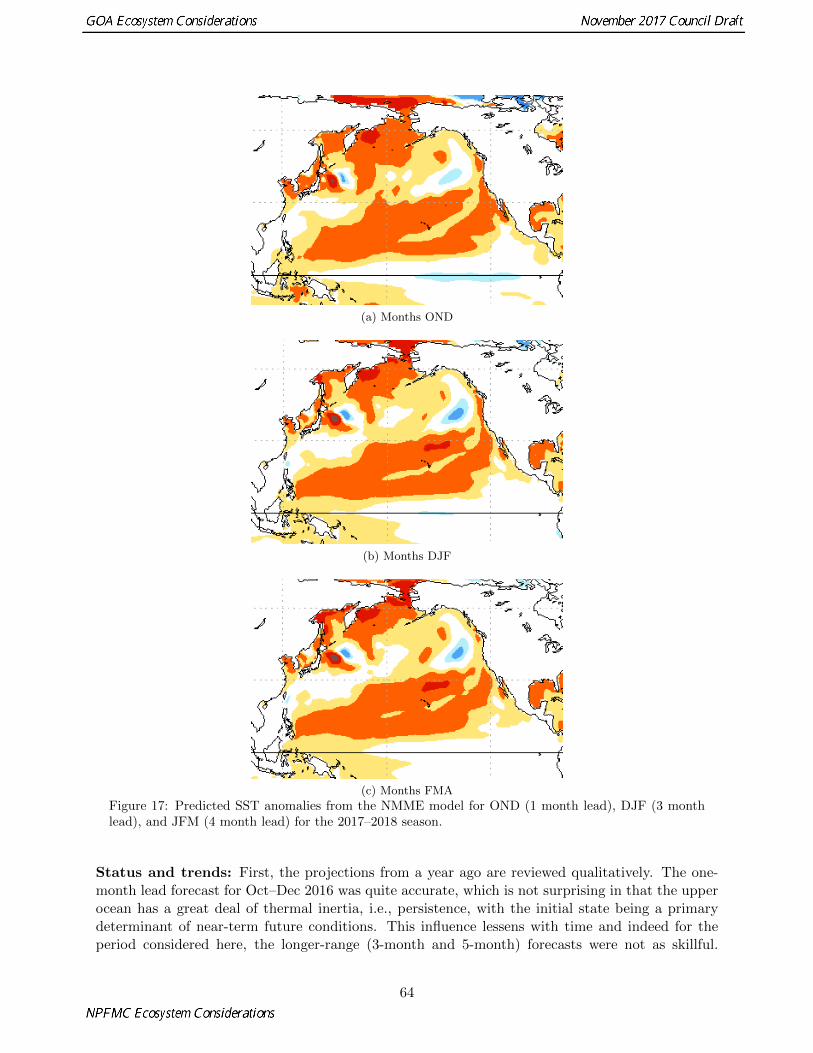
http://www.cpc.ncep.noaa.gov/products/NMME/

(a) Months OND

(b) Months DJF

(c) Months FMA

Figure 17: Predicted SST anomalies from the NMME model for OND (1 month lead), DJF (3 monthlead), and JFM (4 month lead) for the 2017–2018 season.

Status and trends: First, the projections from a year ago are reviewed qualitatively. The one-month lead forecast for Oct–Dec 2016 was quite accurate, which is not surprising in that the upperocean has a great deal of thermal inertia, i.e., persistence, with the initial state being a primarydeterminant of near-term future conditions. This influence lessens with time and indeed for theperiod considered here, the longer-range (3-month and 5-month) forecasts were not as skillful.

64

The models as a group, as reflected in the ensemble averages, correctly predicted the signs andthe magnitudes of the SST anomalies in the sub-tropical and tropical Pacific, with only minordiscrepancies. The NMME forecasts at the 3-month and 5-month forecast horizons did not validateas well north of about 30oN, where the modeled SSTs were generally warmer than observed. Themodels simulated too-little moderation of the pre-existing warm anomalies in the GOA and BeringSea, and also under-predicted the amount of cooling in the waters offshore of the Pacific Northwest.Nevertheless, the models did reproduce the overall patterns in anomalous SST that were observed,even in the longer-range projections; the positive skill in these forecasts discussed here (and foundin other studies) suggest that the NMME SST output merits consideration.

These NMME forecasts of three-month average SST anomalies indicate a continuation of warmconditions across most of the North Pacific through the end of the year (Oct–Dec 2017) with areduction in the longitudinal extent of cooler than normal temperatures offshore of the PacificNorthwest (Figure 17a). The magnitude of the positive anomalies is projected to be greatest(exceeding 1oC) in the western Bering Sea. Negative SST anomalies are projected in the centraland eastern equatorial Pacific. It is uncertain whether they will remain weak enough to constituteneutral conditions or become strong enough to constitute La Nina. As of early September 2017, theprobabilistic forecast provided by NOAA’s Climate Prediction Center (CPC) in collaboration withthe International Research Institute for Climate and Society (IRI) for the upcoming fall throughwinter indicates about a 40% chance of neutral conditions and a 55% chance of a weak La Nina.The overall pattern of SST anomalies across the North Pacific is maintained through the 3-monthperiods of December 2017–February 2018 (Figure 17b) and February–April 2018 (Figure 17c) withsome slight cooling in the eastern Bering Sea, GOA, and nearshore waters of the Pacific Northwest.

Implications The distribution of forecast SST anomalies projects on the positive phase of thePDO, but also exhibits some substantial differences with the characteristic pattern of the PDO.In particular, the positive phase of the PDO generally includes significantly warmer than normalwater in the GOA, and only modest anomalies in the western Bering Sea, while just the reverse isshown in the forecasts. This discrepancy appears to be related to some of the individual NMMEmodels forecasts of a relatively weak Aleutian low (not shown).

Eddies in the Gulf of Alaska

Contributed by Carol Ladd, Pacific Marine Environmental Laboratory, NOAA, Seattle, WABuilding 3, 7600 Sand Point Way NE, Seattle, WA 98115-6349Contact: [email protected] updated: August 2017

Description of indicator: Eddies in the northern Gulf of Alaska have been shown to influence dis-tributions of nutrients (Ladd et al., 2009, 2005; Ladd, 2007), phytoplankton (Brickley and Thomas,2004), ichthyoplankton (Atwood et al., 2010), and the foraging patterns of fur seals (Ream et al.,2005). Eddies propagating along the slope in the northern and western Gulf of Alaska are generallyformed in the eastern Gulf in autumn or early winter (Okkonen et al., 2001) sometimes associatedwith gap winds from Cross Sound (Ladd and Cheng, 2016). Using altimetry data from 1993 to2001, Okkonen et al. (2003) found that strong, persistent eddies occurred more often after 1997than in the period from 1993 to 1997. Ladd et al. (2007) extended that analysis and found that, in

65

the region near Kodiak Island (Figure 18; region c), eddy energy in the years 2002–2004 was thehighest in the altimetry record.

Since 1992, a suite of satellite altimeters has been monitoring sea surface height. Eddy kineticenergy (EKE) can be calculated from gridded altimetry data (merged TOPEX/Poseidon, ERS-1/2, Jason and Envisat; (Ducet et al., 2000), giving a measure of the mesoscale energy in thesystem. A map of eddy kinetic energy in the Gulf of Alaska averaged over the altimetry record(updated from Ladd et al. (2007)) shows four regions with local maxima (labeled a, b, c and din Figure 18). The first two regions are associated with the formation of Haida (a) and Sitka (b)eddies. Eddies that move along the shelf-break often feed into the third and fourth high EKEregions (c and d; Figure 18). By averaging EKE over regions c and d (see boxes in Figure 18), weobtain an index of energy associated with eddies in these regions (Figure 19). The Ssalto/Duacsaltimeter products were produced and distributed by the Copernicus Marine and EnvironmentMonitoring Service (CMEMS) (http://www.marine.copernicus.eu).

Figure 18: Eddy Kinetic Energy averaged over January 1993–December 2016 calculated from satellitealtimetry. Regions (c) and (d) denote regions over which EKE was averaged for Figure 19.

Status and trends: The seasonal cycle of EKE averaged over the two regions (c and d) are outof phase with each other. Region (c) exhibits high EKE in the spring (March–May) and lowerEKE in the autumn (September–November) while region (d) exhibits high EKE in the autumn andlow EKE in the spring. EKE was particularly high in region (c) in 2002–2004 when three largepersistent eddies passed through the region. The highest EKE observed in region (c) occurred in2016 when a strong persistent eddy remained in the region for multiple months. In region (d),high EKE was observed in 1993, 1995, 2000, 2002, 2004, 2006, 2007, 2010, 2012, 2013, and 2015.Near-real-time data suggests that EKE was low in both regions in spring and summer 2017. Thehigh EKE values in spring 2016 in region (c) were due to a strong eddy that formed near Yakutatin January 2016.

66

http://www.marine.copernicus.eu

Figure 19: Eddy kinetic energy (cm2 s-2) averaged over Region (d) (top) and Region (c) (bottom) shownin Figure 18. Black (line with highest variability): monthly EKE (dashed part of line is from near-real-time altimetry product which is less accurate than the delayed altimetry product), Red: seasonal cycle.Green (straight line): mean over entire time series.

Factors causing observed trends: In the eastern Gulf of Alaska, interannual changes in surfacewinds (related to the Pacific Decadal Oscillation, El Nino), and the strength of the Aleutian Lowmodulate the development of eddies (Combes and Di Lorenzo, 2007; Di Lorenzo et al., 2013).Recent work suggests that regional scale gap-wind events may also play a role in eddy formationin the eastern Gulf of Alaska (Ladd and Cheng, 2016). In the western Gulf of Alaska, variability isrelated both to the propagation of eddies from their formation regions in the east and to intrinsicvariability.

Implications: EKE may have implications for the ecosystem. Phytoplankton biomass was proba-bly more tightly confined to the shelf during 2017 due to the absence of eddies, while in 2007, 2010,2012, 2013, and 2015 (region (d)), phytoplankton biomass likely extended farther off the shelf. Inaddition, cross-shelf transport of heat, salinity, and nutrients were probably weaker in 2017 thanin years with large persistent eddies. Eddies sampled in 2002–2004 were found to contain differentichthyoplankton assemblages than surrounding slope and basin waters indicating that eddies alongthe slope may influence the distribution and survival of fish (Atwood et al., 2010). In addition,carbon isotope values suggest that cross-shelf exchange due to eddies may be important to themarine survival rate of pink salmon (Kline, 2010).

Ocean Surface Currents – Papa Trajectory Index

Contributed by William T. StockhausenResource Ecology and Fishery Management Division, Alaska Fisheries Science Center, NationalMarine Fisheries Service, NOAAContact: [email protected]

67

Last updated: August 2017

Description of indicator: The PAPA Trajectory Index (PTI) provides an annual index of near-surface water movement variability, based on the trajectory of a simulated surface drifter releasedat Ocean Station PAPA (50oN, 145oW; Figure 20). The simulation for each year is conductedusing the “Ocean Surface CURrent Simulator” (OSCURS; http://las.pfeg.noaa.gov/oscurs).Using daily gridded atmospheric pressure fields, OSCURS calculates the speed and direction ofwater movement at the ocean’s surface at the location of a simulated surface drifter. It usesthis information to update the position of the simulated drifter on a daily basis over a specifiedtime period. For the index presented here, OSCURS was run for 90 days to simulate a surfacedrifter released at Ocean Station PAPA on December 1 for each year from 1901 to 2016 (trajectoryendpoints years 1902–2017).

2016

2017

2015

2014

2013

2012

PAPA

2008

2009

2010

2011

Sources: Esri, GEBCO, NOAA, National Geographic, DeLorme, HERE, Geonames.org, and othercontributors

130°W

140°W

140°W

150°W

150°W

60°N

55°N

55°N

50°N

50°N

Figure 20: Simulated surface drifter trajectories for winters 2008–2017 (endpoint year). End pointsof 90-day trajectories for simulated surface drifters released on Dec. 1 of the previous year at OceanWeather Station PAPA are labeled with the year of the endpoint (50oN, 145oW).

Status and trends: In general, the trajectories fan out northeastwardly toward the North Amer-ican continent (Figure 20). The 2009/2010 trajectory was an exception and resulted in the west-ernmost trajectory endpoint for the entire set of model runs (1902–2017 endpoints). Under the

68

http://las.pfeg.noaa.gov/oscurs

influence of contemporaneous El Nino conditions, the Aleutian Low in the winter of 2009–2010 wasanomalously deep and displaced to the southeast of its usual position in winter (Bond and Guy,2010), resulting in anomalously high easterly (blowing west) wind anomalies north of Ocean Sta-tion PAPA. The 2011/2012 trajectory followed the general northeastwardly path of most drifters,but was notable because its ending latitude was the northernmost of all trajectories since 1994.The trajectory for 2012/13 was notable as ending up the furthest east among trajectories in re-cent years, driven by very strong westerly anomalies in the northeast Pacific. The trajectoriesfor 2013/14, 2014/15, and 2015/16 trajectories were very similar to that for 2011/12, althoughthese did not reach quite as as far north as in 2011/12. These trajectories coincided with thedevelopment (2013/14) and continuation (2014/15, 2015/16) of the “Blob” of warm surface watersalong the eastern Pacific coast and the return of the Pacific Decadal Oscillation (PDO) to a warm,positive phase associated with winds from the south near the coast. The increased southerly windscontributed to well above-average sea surface temperatures in the Gulf of Alaska in 2015/16. Theopposite was true for the 2016/17 winter, however, and strong northerly winds pushed the driftertrajectory to its most southerly latitude since the late 1930s.

Figure 21: Annual, long-term mean (green line), and 5-year running mean (red line and squares) of thePAPA Trajectory Index time series (dotted black line and points) for 1902–2017 winters.

The PTI time series (Figure 21, black dotted line and points) indicates high interannual variationin the north/south component of drifter trajectories, with an average between-year change of >4o

and a maximum change of greater than 13o (between 1931–1932). The change in the PTI between2010/11 and 2011/12 was the largest since 1994, while the changes between 2011/12 and 2012/13,and between 2012/13 and 2013/14, represented reversals with slightly less, but diminishing, mag-nitude. Such swings, however, were not uncommon over the entire time series. The changes from2013/14 to 2015/16 constituted a relatively rare event when the index changed very little over threesuccessive years.

Over the past century, the filtered (5-year running average) PTI has undergone four completeoscillations with distinct crossings of the mean, although the durations of the oscillations are not

69

identical: 26 years (1904–1930), 17 years (1930–1947), 17 years (1947–1964), and 41 years (1964–2005). The filtered index indicates that a shift occurred in the mid 2000s to predominantly southerlyanomalous flow following a 20+ year period of predominantly northerly anomalous flow. This wasindicative of a return to conditions (at least in terms of surface drift) similar to those prior to the1977 environmental regime shift. This part of the cycle apparently ended rather quickly, however,as it now appears the filtered PTI has crossed the mean in the opposite direction. The recentperiod of predominantly southern flow has been the shortest and weakest in the time series.

Factors influencing observed trends: Filtered PTI values greater than the long-term mean areindicative of increased transport and/or a northerly shift in the Alaska Current, which transportswarm water northward along the west coast of Canada and southeast Alaska from the south andconsequently plays a major role in the Gulf of Alaskas heat budget. In addition, the PDO recently(July, 2014) shifted into a positive and warm phase, associated with warm SST anomalies near thecoast in the eastern Pacific and low sea level pressures over the North Pacific, the latter of whichcontributes to southerly winds and northerly flows. Individual trajectories also reflect interannualvariability in regional (northeast Pacific) wind patterns.

Implications: The year-to-year variability in near-surface water movements in the North Pa-cific Ocean has been shown to have important effects on the survival of walleye pollock (Gaduschalcogrammus) by affecting its spatial overlap with predators (Wespestad et al., 2000), as well asto influence recruitment success of winter spawning flatfish in the eastern Bering Sea (EBS; Wilder-buer et al. (2002)). Interdecadal changes in the PTI reflect changes in ocean climate that appearto have widespread impacts on biological variability at multiple trophic levels (King, 2005). Thereis strong evidence that the productivity and possibly the carrying capacity of the Alaska Gyre andof the continental shelf were enhanced during the “warm” regime that began in 1977. Zooplanktonproduction was positively affected after the 1977 regime shift (Brodeur and Ware, 1992), as wererecruitment and survival of salmon and demersal fish species. Recruitment of rockfish (Pacificocean perch) and flatfish (arrowtooth flounder, halibut, and flathead sole) also increased. However,shrimp and forage fish such as capelin were negatively affected by the 1977 shift (Anderson, 2003).The reduced availability of forage fish may have contributed to the decline in marine mammal andseabird populations observed after the 1977 shift (Piatt and Anderson, 1996).

Gulf of Alaska Survey Bottom Trawl Temperature Analysis

Contributed by Ned Laman, Resource Assessment and Conservation Engineering Division, Ground-fish Assessment Program, Alaska Fisheries Science Center, National Marine Fisheries Service,NOAAContact: [email protected] updated: October 2017

Description of indicator: Since 1993, water column temperatures have been routinely recordedduring Alaska Fisheries Science Center (AFSC) Resource Assessment and Conservation Engineer-ing Groundfish Assessment Program (RACE-GAP) GOA bottom trawl surveys using bathythermo-graph data loggers attached to the headrope of the bottom trawl net. In 2003, the SeaBird (SBE-39)microbathythermograph (Sea-Bird Electronics, Inc., Bellevue, WA) replaced the Brancker XL200data logger (Richard Brancker Research, Ltd., Kanata, Ontario, Canada) which had been in use

70

from 1993–2001 (Buckley et al., 2009). The analyses presented here combine these two types ofbathythermic data; the downcast data from each RACE-GAP trawl haul were isolated and used toinform our models.

The spatial and temporal coverage of the GOA RACE-GAP summer bottom trawl surveys hasvaried from year to year. Starting dates have ranged from the middle of May to the first week inJune, and survey end dates ranged from the third week in July to the first week in September. Thenumber of vessels employed, the areal extent, and the maximum depth of the GOA survey have allvaried between survey years (e.g., water temperatures were not collected from the eastern GOA in1993 and 2001, stations in the deepest GOA stratum [700–1000 m] have been sampled in just 5 ofthe last 12 surveys). Additionally, there is the expectation of an overall warming trend for watertemperatures collected as the summer advances and the bottom trawl survey progresses from thewestern GOA into southeast Alaska; this should be particularly pronounced in the upper layers ofthe water column.

To account for the spatio-temporal variation that were a consequence of the survey design weremoved the effect of collection date on water temperature by standardizing all RACE-GAP GOAbottom trawl collection dates to a median survey date of July 10. We formulated a generalizedadditive model (GAM) to estimate the effects of collection date on temperature at depth acrosssurvey areas and years; the GAM accounted for 81% of the total deviance in the temperature data.The resulting model was used to predict water temperature on the median survey day at depth andstation from survey trawl haul downcasts. Model residuals were added to the predicted median daytemperature-at-depth to produce temperature anomaly estimates for each station and depth duringeach survey year. To facilitate visualization, these estimates were averaged over systematic depthbins in 1⁄2-degree longitude increments. Depth gradations were set finer in shallower depths (e.g., 5m bins between 0 and 100 m, 10 m bins between 100 and 300 m) to capture the anticipated rapidwater temperature changes in surface waters with increasing depth. To further stretch the colorramp and enhance the visual separation of the near-surface temperature anomalies (between ∼ 4and 10oC and < 100 m), predicted temperature anomalies ≥ 9.5oC and ≤ 3.5oC were fixed at 9.5and 3.5oC (e.g., a 12.5oC temperature anomaly was recoded as 9.5oC for the graphic representation)and the y-axis (depth) was truncated (0–400 m) relative to the deepest depths sampled (ca. 1000m).

Status and trends: The thermal profile suggests that conditions in 2017 may have been slightlycooler compared to 2015 but still among the warmer years in our record (Figure 22). The warmestwater did not penetrate as deeply into the upper 100 m in 2017. The warmer anomalies from thissummers survey (≥ 7oC) were generally constrained to depths < 50 m whereas similar temperatureanomaly values in 2015 were common between 50 and 100 m. However, there appeared to bewarmer water deeper in the central Gulf (200–300 m) in 2017 compared to 2015. In general, the2017 GOA thermal profile shares characteristics of the other warm years in our record (i.e., 2003,2005, and 2015) and contrasts with the cooler years we have observed (e.g., 2007–2013).

Factors influencing observed trends: Temperature data we collected during RACE-GAP bot-tom trawl surveys in the GOA represent a temporally brief and spatially constrained snapshot ofwater column conditions. In the data summarized in the figure, each temperature bin representsdata that were collected over a relatively short time as the vessels moved through the area. It isdifficult to draw general conclusions about longer term trends from this type of data, especiallysince these temperature observations can be affected by short term events such as storms, tidalcurrents, and changes in freshwater discharge. More persistent medium-term phenomena like sea-

71

sonal changes in solar heat flux, El Nino Southern Oscillations, and shifts in the Alaska CoastalCurrent also play an important role in determining water column temperatures. In addition, thestrength and persistence of eddies are believed to have a large impact on the transport of both heatand nutrients across the continental shelf in the GOA (Ladd et al., 2007). The data reported heredepict the variation in water column temperatures observed amongst GOA bottom trawl surveyyears, but do not inform the mechanisms or processes driving these differences.

Implications: Water column temperatures influence the distribution, assemblage membership,abundance, and growth rates of phytoplankton and zooplankton species. Ichthyoplankton distri-bution and growth rates are also related to location of the warm core eddies that are a prominentfeature of the central GOA (Atwood et al., 2010). Adult and juvenile fish distribution can alsobe influenced by water temperatures (Kotwicki and Lauth, 2013; Rooney et al., in press). Inter-annual differences in water column temperatures, their implications, and their possible effects onfish populations in the GOA require more study to be better understood.

72

Figure 22: Temperature (oC) anomaly profiles derived from RACE-GAP Gulf of Alaska bottom trawlsurvey bathythermograph casts (1993–2017) and predicted from a generalized additive model at system-atic depth increments and 1⁄2-degree longitude intervals; to visually enhance near-surface temperaturechanges, values ≤ 3.5oC or ≥ 9.5oC were fixed at 3.5 or 9.5oC and the y-axis (depth) was truncated at400 m (relative to maximum collection depth ca 1000 m).

73

Temperature and Salinity at GAK1

Contributed by Seth Danielson, College of Fisheries and Ocean Sciences, University of Alaska,Fairbanks, AKContact: [email protected] updated: September 2017

Description of indicator: Temperature and salinity versus depth profiles have been taken sinceDecember 1970 at oceanographic station GAK1, located at the mouth of Resurrection Bay nearSeward, Alaska. This 47-year time series is one of the longest running oceanographic time seriesin the North Pacific and the longest-running hydrographic profile dataset in Alaskan waters. Thelocation is 59o 50.7’ N, 149o 28.0’ W and is located within the Alaska Coastal Current, so it is well“connected” with the shelf circulation. The sampling platform is normally R/V Little Dipper, a28’ coastal research vessel operated by the University of Alaskas Seward Marine Center.

The goal of the GAK1 project is to provide a long-term high-quality reference dataset for thecoastal northern Gulf of Alaska that enables scientists, students, commercial and subsistence fishersand resource managers to better understand climatic and ecological conditions, their changes,and ramifications of change. Understanding, anticipating, and responding to change requires astationary frame of reference in the form of long-term in situ observations. Such datasets arethe best means to guide our assessments and interpretations of system variability. Untangling therelations between climatic and other drivers of change (e.g., oil spills or fishing regulations) similarlyrequires long reference time series. Environmental time series data can provide information valuableto the management of fish and shellfish populations and fisheries.

The GAK1 dataset is collected under the fundamental hypothesis that oceanic conditions areimportant to the physical and biological functioning of the Prince William Sound and Gulf of Alaskaecosystems. To that end, many dozens of papers have examined this hypothesis from numerousperspectives (for a comprehensive listing, see the GAK1 home page at http://www.ims.uaf.edu/gak1/). As the chemical and biological datasets begin to catch up (via quality of resolution,duration and frequency) to the physical measurements we expect that the insights gleaned throughinterdisciplinary analyses will grow in kind.

Status and trends: Year 2016 was the warmest on record for the GAK1 time series. Trendsshown in Figure 23 are averages over 0–50 m depth and 200–250 m depth. Table 2 shows regressionstatistics for the period of record and for 2009–2016. The recent 2013–2016 warm interval waspreceded by relatively cool temperatures over 2007–2012 and as a consequence the 2009–2016analysis period shows an increasing trend that is an order of magnitude larger than the 1970–2016interval. While salinity has declined in the past decade in both the near-surface and near-bottom,salinity over the entire time period has increase slightly in the near-bottom.

Factors influencing observed trends: The GAK1 record captures long-term (47-year) trendsof warming throughout the water column, along with freshening in the 50 m closest to the surfaceand a slight salinization close to the seafloor. The observed warming is consistent with long-termclimate trends of warming for the planet as a whole. Warming temperatures affect snow melt, netglacial ablation, coastal runoff, and by extension, these terrestrial discharges impact the surfacesalinity. The reasons for the near-seafloor salinity increases are presently unknown and are underinvestigation.

74

http://www.ims.uaf.edu/gak1/

http://www.ims.uaf.edu/gak1/

Figure 23: Plots of temperature (left) and salinity (right) monthly anomalies over 1970–2016. Blacklines depict the least squares best-fit line to the data.

Implications: There are myriad consequences that may propagate through the ecosystem as aresult of the observed temperature and salinity changes and many effects are difficult or impossibleto anticipate. Some expected impacts include the following: 1. increasing coastal salinities couldincrease the along-shelf transport in the Alaska Coastal Current, altering the dispersal pathwaysand/or timing of water, heat, the coastal water chemical constituents, and plankton that are in-fluenced by the coastal current; 2. warming will lead to increased metabolic rates and changes inbiogeochemical cycling; 3. differential trends in the influence of temperature and salinity lead toincreased levels of stratification on the Gulf of Alaska continental shelf; and 4. increasing stratifica-tion may alter (reduce) the transfer of nitrate from subsurface waters into the euphotic zone. Thelatter has implications for the amount of new production that the shelf may be able to sustain.

Watershed Dynamics in the Auke Creek System, Southeast Alaska

Contributed by Scott C. Vulstek and Joshua R. RussellAuke Bay Laboratories Division, Alaska Fisheries Science Center, National Marine Fisheries Ser-vice, NOAAContact: [email protected] updated: September 2017

Description of indicator: The Auke Creek Research Station has been in permanent operationsince 1980 and provides a unique opportunity to study migratory salmonids due to the operation of

75

Table 2: Regression statistics for temperature and salinity at GAK1 from 1970–2016.

ParameterDaterange

DepthRange(m)

Numberofsamples

Trend(perdecade)

TrendConfidencebounds

Correlationcoefficient

p-value

Temperature (C) 1970-2016 0-50 381 0.24 +/- 0.068 0.11 1.07E-11Temperature (C) 1970-2016 200-250 379 0.15 +/- 0.040 0.13 1.08E-12Temperature (C) 2009-2016 0-50 93 2.93 +/- 0.704 0.43 1.05E-12Temperature (C) 2009-2016 200-250 93 1.39 +/- 0.322 0.45 2.31E-13Salinity 1970-2016 0-50 381 -0.08 +/- 0.035 0.05 7.99E-06Salinity 1970-2016 200-250 379 0.02 +/- 0.019 0.01 6.53E-02Salinity 2009-2016 0-50 93 -0.78 +/- 0.323 0.20 5.77E-06Salinity 2009-2016 200-250 93 -0.12 +/- 0.233 0.01 3.10E-01

a weir capable of the near-perfect capture of all migrating juvenile and adult salmon. In addition tothe capture of migrating individuals, daily recordings of environmental variables are also collected.These variables include: creek temperature, and creek height. Creek temperature is collected usingan in-creek probe that records temperature on an hourly basis and is located 25 meters upstreamof the weir structure. Creek height is recorded using a staff gauge that is permanently installeddirectly downstream of the weir structure and approximately 7 meters above the average low tideline. Thirty-eight years of temperature data are available (1980–2017), and 12 years of creek heightdata (2006–2017). These variables provide a valuable addition to the fisheries data collected at theAuke Creek Research Station.

Status and trends: The historical trends of yearly average creek temperature in Auke Creekvaries from 8.6oC to 11.6oC with an average temperature of 10.3oC from 1980–2017. The averagetemperature for 2016 was 11.5oC and 10.4oC for 2017. From 2006–2017, average yearly creek heightvaried from 21.6ft to 21.9ft, with an average of 21.7 ft. The average gauge height for 2017 was21.6ft and 21.8ft for 2017. Historical trends and the most recent two years are shown for creektemperature (Figure 24) and gauge height (Figure 25).

Factors influencing observed trends: The trends that we are observing in the Auke Creekwatershed provide further evidence for the rapid climatic change that has been documented inthis system. Due to recent fluctuations in winter snowfall, we are seeing shifts from a snowmelt-dominated to a rainfall-dominated watershed at Auke Creek (Shanley et al., 2015)(Figure 25). Thislack of snowfall, and subsequent lack of snowmelt, contribute to warmer creek temperatures earlierin the year (Figure 24).

Implications: These changes in stream conditions and climate have been shown to have influenceon the median migration date of juvenile and adult salmon in Auke Creek (Kovach et al., 2013). Ad-ditionally, changes in time of entry to the marine environment can effect marine survival (Weitkampet al., 2011). Both of these can have impacts on groundfish and salmon productivity as juvenilesalmon serve as an important food source in the early marine environment. (Landingham et al.,1998; Sturdevant et al., 2009, 2012). Additionally, shifts in the timing and magnitude of freshwaterand associated nutrient input directly affects processes in the nearshore marine environment (e.g.,salinity and temperature).

76

Figure 24: Auke Creek average temperature by months of operation for 1980–2015, 2016, and 2017.

Figure 25: Auke Creek average gauge height by months of operation for 2006–2015, 2016, and 2017.

77

Habitat

Structural Epifauna – Gulf of Alaska

Contributed by Chris Rooper, Resource Assessment and Conservation Engineering Division, AlaskaFisheries Science Center, National Marine Fisheries Service, NOAAContact: [email protected] updated: October 2017

Description of indicator: Structural epifauna groups considered to be Habitat Area of ParticularConcern (HAPC) biota include sponges, corals (both hard and soft) and anemones. NOAA collectsdata on structural epifauna during the biennial RACE summer surveys in the Gulf of Alaska.For each species group, the catches for each year were scaled to the largest catch over the timeseries (which was arbitrarily scaled to a value of 100). The standard error (±1) was weightedproportionally to the CPUE to get a relative standard error. The percentage of positive catches inthe survey bottom trawl hauls was also calculated.

Status and trends: A few general patterns are clearly discernible (Figure 26). Sponges are caughtin about 50% of bottom trawl survey hauls in all areas of the GOA when combined across areas.This percentage has been increasing in the Yakutat (to about 30% of hauls) and Southeastern (toabout 60% of hauls) regions. However, the CPUE is generally highest in the Shumagin area low tothe east. Sponge CPUE has declined in the Kodiak area, while CPUE has remained fairly constantin the four other areas. Anemones are caught in low abundance in the eastern GOA, while they arecommon (occur in ∼50% of tows) at a relatively constant abundance in the Shumagin, Chirikof andKodiak regions. Gorgonian corals show an opposite pattern, as they are in highest abundance inthe southeastern GOA, although they are relatively uncommon in catches for all areas. The peakabundance occurred in 1999 in the eastern GOA, and catches have declined in recent surveys. Thesea pen time series is dominated by large CPUEs in 2005 and 2015 in the Chirikof area, but theyoccur uncommonly in bottom trawl tows (< 10% occurrence). Stony coral catches are rare. Softcoral CPUE has been uniformly low with the exception of a large catch in the western GOA in the1984 survey.

78

Figure 26: Mean CPUE of HAPC species groups by area from RACE bottom trawl surveys in the Gulf of Alaska from 1984 through 2017. Errorbars represent standard errors. The gray lines represent the percentage of non-zero catches.

79

Factors influencing observed trends: The Gulf of Alaska survey does not sample any of thesefauna well, so some caution is recommended in interpreting these trends in CPUE. Overall, mostarea-species combinations do not show trends in either catches or frequency of occurrence. However,the decline in sponge catches in the Kodiak area may indicate that sponges are decreasing here,whereas the increases in frequency of occurrence of sponges in the Yakutat and Southeastern areasmay indicate an expansion of sponge populations.

Implications: Changes in structural epifauna CPUE may indicate changes in habitat, but atpresent no research has demonstrated definitive links. In future ecosystem contributions an overallbiomass for these species groups for the Gulf of Alaska will be computed using geospatial methods.Preliminary results (Figure 27) show that overall coral and sponge biomass estimates have remainedhighly variable, but relatively constant throughout the history of the bottom trawl survey, whereaspennatulaceans seemed to peak in the 2005 survey before falling off and recovering to a high levelin 2017. These are preliminary results and need further examination and exploration.

Primary Production

There are no updates to primary production indicators in this year’s report, except for the diatomtrends in the Continuous Plankton Recorder contribution by Batten (p. 80. See the contribu-tion archive for previous indicator submissions at: http://access.afsc.noaa.gov/reem/ecoweb/index.php

Zooplankton

Continuous Plankton Recorder Data from the Northeast Pacific: Lower Trophic Levelsin 2016

Contributed by Sonia Batten, Sir Alister Hardy Foundation for Ocean Science, c/o 4737 Vista ViewCr, Nanaimo, BC, V9V 1N8, CanadaContact: [email protected] updated: July 2017

Description of indicator: Continuous Plankton Recorders (CPRs) have been deployed in theNorth Pacific routinely since 2000. Two transects are sampled seasonally, both originating in theStrait of Juan de Fuca, one sampled monthly (∼Apr–Sept) which terminates in Cook Inlet, thesecond sampled 3 times per year (in spring, summer and autumn) which follows a great circleroute across the Pacific terminating in Asia. Several indicators are now routinely derived fromthe CPR data and updated annually. In this report we update three indices for three two regions(Figure 28); the abundance per sample of large diatoms (the CPR only retains large, hard-shelledphytoplankton so while a large proportion of the community is not sampled, the data are internallyconsistent and may reveal trends), mesozooplankton biomass (estimated from taxon-specific weightsand abundance data) and mean Copepod Community Size (see Richardson et al., 2006 for detailsbut essentially the length of an adult female of each species is used to represent that species andan average length of all copepods sampled calculated) as an indicator of community composition.Anomaly time series of each index have been calculated as follows: A monthly mean value for each

80



Figure 27: Time series of structure forming invertebrate biomass estimates for the Gulf of Alaska.Estimates (and standard deviations) were produced using a multispecies VAST model that includedcombined coral groups, combined pennatulaceans and combined sponge groups.

region is first calculated. Each sampled months mean is then compared to the long-term mean ofthat month and an anomaly calculated (Log10). The mean anomaly of all sampled months in eachyear is calculated to give an annual anomaly.

The indices are calculated for the oceanic North-East Pacific and the Alaskan shelf SE of CookInlet (Figure 28). The oceanic NE Pacific region has the best sampling resolution as both transects

81

intersect here. This region has been sampled up to 9 times per year with some months sampledtwice. The Alaskan shelf region is sampled 5–6 times per year by the north-south transect.

Figure 28: Boundaries of the regions described in this report. Dots indicate actual sample positions(note that for the Alaskan Shelf region the multiple (>50) transects overlay each other almost entirely).The Southern Bering Sea region is not discussed in this report.

Status and trends: Diatom abundance anomalies were very low on the Alaskan Shelf in 2016(particularly in April and May) and lower than in 2015 in the oceanic NE Pacific (Figure 29).The mesozooplankton biomass anomaly was strongly positive on the Alaskan shelf, with positiveanomalies in each sampled month. It was also positive overall for the NE Pacific region, althoughMay and July values were slightly negative. The Copepod Community Size index saw negativeanomalies for both the Alaskan Shelf and the NE Pacific regions meaning that the species weresmaller then average. For the Alaskan Shelf region this was the 4th consecutive year of negativeanomalies and while the anomaly for the NE Pacific was not as low as in 2015, it was again negative.

Factors influencing observed trends: We have previously speculated that during the previousheat wave years of 2014–2015 nutrient conditions may have been poor since a higher than averagecontribution of smaller, pennate diatoms (that have an advantage over larger cells in low nutrientconditions) was evident in spring of those years in the Alaskan Shelf, as well as the NE Pacific region.This trend could have continued with even smaller cells present in 2016 that are not retained by theCPR. However, there was a very high zooplankton biomass in 2016 so it is also possible that thelow numbers of larger diatoms was caused by high grazing pressure from zooplankton. Whateverthe cause, the diatom anomaly in spring 2016 was the lowest of the time series so clearly somethingwas unusual in the 2016 plankton community.

The negative anomalies for the Copepod Community Size Index for both the Alaska Shelf andNE Pacific regions are consistent with the warmer water favoring the smaller-bodied species whichgenerally have a more southerly center to their distribution and are more abundant in warm years.They were very abundant in 2016, since biomass anomalies were positive while mean size was small.

Implications: Each of these variables is important to the way that ocean climate variability ispassed though the phytoplankton to zooplankton and up to higher trophic levels. Changes in

82

Figure 29: Annual anomalies of three indices of lower trophic levels (see text for description and deriva-tion) for each region shown in (Figure 28). Note that sampling of this Alaskan Shelf region did notbegin until 2004.

community composition (e.g., abundance and composition of large diatoms, prey size as indexedby mean copepod community size) may reflect changes in the nutritional quality of the organism totheir predators. Changes in abundance or biomass, together with size, influences availability of preyto predators. For example, while mesozooplankton biomass anomalies were positive, the reducedaverage size of the copepod community suggests that the biomass was packaged into numerous, butsmall, prey items. This may require more work by predators to obtain their nutritional needs, andfor the Alaskan Shelf region this is now a persistent feature occurring in 4 consecutive years.

Rapid Zooplankton Assessment and Long-Term Time Series, Western Gulf of Alaska,Spring and Summer 2017

Contributed by Nissa Ferm, Jesse Lamb, David Kimmel, EcoFOCI Program, Resource Assessmentand Conservation Engineering Division, Alaska Fisheries Science Center, National Marine FisheriesService, NOAAContact: [email protected]

83

Last updated: September 2017

Description of indicator: In 2015, EcoFOCI implemented a method for an at sea Rapid Zoo-plankton Assessment (RZA) to provide leading indicator information on zooplankton compositionin Alaska’s Large Marine Ecosystems. The rapid assessment, which is a rough count of zooplank-ton (from paired 20/60 cm oblique bongo tows from 10 m from bottom or 300 m, whichever isshallower), provides preliminary estimates of zooplankton abundance and community structure.The method employed uses coarse categories and standard zooplankton sorting methods (Harriset al., 2005). The categories are small copepods (< 2 mm; example species: Acartia spp., Pseu-docalanus spp. and Oithona spp.), large copepods (> 2mm; example species: Calanus spp. andNeocalanus spp.), and euphausiids (< 15 mm; example species: Thysanoessa spp.). Small cope-pods were counted from the 153 µm mesh, 20 cm bongo net. Large copepods and euphausiids werecounted from the 505 µm mesh, 60 cm bongo net. In 2016, the method was refined and personnelcounted a minimum of 100 organisms per sample at sea to improve zooplankton estimates. Other,rarer zooplankton taxa were present but were not sampled effectively with the on-board samplingmethod. Detailed information on these taxa is provided after in-lab processing protocols have beenfollowed (1+ years post survey). The GOA RZA was conducted on two surveys: 1) from 12 Mayto 1 June 2017 (spring) and 2) from 19 Aug to 17 Sep 2017 (summer).

In order to provide comparison to yearly RZA data, a long-term time series was developed fromarchived data. The mean, annual abundance of each RZA category was plotted for “Line 8” (anarea approximately bounded by 57.46–57.73oN and 154.67–155.30oW) in the Shelikof Strait, Gulf ofAlaska from 1990–2011 and represented May/June sampling (spring). For summer, mean, annualabundance of each RZA category was plotted for the primary grid area southwest of Kodiak Island(an area approximately bounded by 54–58oN and 155–160oW) from 2000–2015 (where data wereavailable) and represented Aug/Sep sampling.

Status and trends: Large copepods had high abundances in the SW area of the survey gridand near Kodiak Island in spring (Figure 30). Large copepod abundances declined in summer,and the SW area of the survey grid remained the area with the highest abundances (Figure 30).Compared to historical abundances of large copepods at Line 8, 2017 abundances appeared to besimilar in magnitude to the long-term estimates and higher than 2015 (Figure 31). Small copepodswere abundant throughout the sampling area in spring, and their abundances increased duringsummer (Figure 30). Small copepods showed very little interannual variability in spring and summerabundance, and 2017 values were similar to the long-term estimates (Figure 31). Euphausiidjuvenile stages were abundant throughout the sampling region in spring and numbers reduced intosummer (Figure 30). Euphausiid abundances appeared to be much higher than historical estimatesin spring in general and 2015 in particular (Figure 31). Higher abundances of euphausiids wereobserved in summer of 2015 and 2017 compared to the most recent survey values (Figure 31).

Factors influencing observed trends: Large copepods in spring include Neocalanus cristatusand N. plumchrus/flemingeri. These species enter diapause and disappear from the plankton inJune, thus the decline of larger copepods into the summer (Figure 30) is partially explained bythis life history event. The other large copepod species, Calanus marshallae, has been shown toincrease in years with cold winters and a strong, spring phytoplankton bloom (Sousa et al., 2016).We observed evidence of a recent spring bloom and numerous Calanus copepodites during thespring survey, suggesting that winter conditions were favorable for Calanus. The long-term times-series of large and small copepods showed little variability in either spring or summer (Figure

84

(a) Large Copepods–Spring (b) Large Copepods–Summer

(c) Small Copepods–Spring (d) Small Copepods–Summer

(e) Euphausiids–Spring (f) Euphausiids–Summer

Figure 30: Maps show the spring (left) and summer (right) abundance of large copepods, small copepods,and euphausiid larvae/juveniles estimated by the rapid zooplankton assessment. Note all maps have adifferent abundance scales (No. m-3). X indicates a sample with abundance of zero individuals m-3.

31) and this is likely due to the combination of multiple species into one, representative category.Examination of individual species shows that variability among the individual species of smallercopepods does occur (unpub. data). We also observed large numbers of euphausiid early life historystages in spring (Figure 30). Sousa et al. (2016) also report the conditions that increased Calanusabundances also appeared to favor the euphausiid Thysanoessa inermis. The significant decline in

85

Figure 2. Spring (left) and summer (right), annual, mean abundance of large copepods, small copepods, and euphausiids in the Gulf of Alaska, FOCI sampling region. Black points and lines represent FOCI archived data from the Line 8 region, blue points represent RZA data from spring sampling across the Gulf of Alaska in 2015 and 2017. Error bars represent standard error of the mean.

Figure 31: Spring (left) and summer (right), annual, mean abundance of large copepods, small copepods,and euphausiids in the Gulf of Alaska, FOCI sampling region. Black points and lines represent FOCIarchived data from the Line 8 region, blue points represent RZA data from spring sampling across theGulf of Alaska in 2015 and 2017. Error bars represent standard error of the mean.

euphausiid numbers during the summer (Figure 30) can be partially explained by the developmentof euphausiids resulting in larger sized individuals that can effectively avoid the 60 cm bongo net.Long-term variability in mesozooplankton in this region is thought to be driven by PDO and ENSOcycles (Sousa et al., 2016). However, the euphausiid variability does show some patterns over time(Figure 31). The drops in euphausiid abundance corresponded with positive phases of the PDO(Figure 31) as suggested by (Sousa et al., 2016). However, considerable local variability within agiven year may mask these longer-term trends in abundance.

Implications: Zooplankton are an important prey base for larval and small juvenile pollock inspring. The increase in abundance of copepods and their presence at nearly all stations indicatessignificant secondary production present in the ecosystem during spring of 2017, particularly whencompared to 2015 estimates (Figure 31). Furthermore, the higher abundances of early stage eu-phausiids present could bode well for higher abundances in fall when juvenile pollock diets shift to

86

a primarily euphausiid-based diet prior to overwintering.

Gulf of Alaska Euphausiid (“krill”) Acoustic Survey

Contributed by Patrick Ressler, Midwater Assessment and Conservation Engineering Program, Re-source Assessment and Conservation Engineering Division, Alaska Fisheries Science Center, NOAAContact: [email protected] updated: October 2017

Description of indicator: The Gulf of Alaska survey of the abundance and distribution ofeuphausiids (“krill”, principally Thysanoessa spp.) has been developed (Simonsen et al., 2016)based on methods used by Ressler et al. (2012) in the Bering Sea. The survey incorporates bothacoustic and Methot trawl data from summer Gulf of Alaska acoustic-trawl surveys for pollockconducted in 2003, 2005, 2011, and biennially since 2013 by NOAA-AFSC. Acoustic backscatter perunit area (sA at 120 kHz, m2 nmi-2) classified as euphausiids was integrated over the water columnand then across the surveyed area to produce an annual estimate of acoustic abundance (sA * area,proportional to the total abundance of euphausiids). Approximate 95% confidence intervals onthese estimates were computed from geostatistical estimates of relative estimation error (Petitgas,1993). Though surveys since 2013 have covered the shelf from the Islands of Four Mountains toYakutat (Figure 32), the index reported here is limited to areas around Kodiak that have beenconsistently sampled in all years of the time series (Figure 33). Net collections from euphausiidscattering layers in 2011, 2013, and 2015 have been numerically dominated by euphausiids and showthat Thysanoessa inermis, T. spinifera, and Euphausia pacifica with average length ∼19 mm are themost commonly encountered species (Simonsen et al. 2016, Ressler unpublished data). Additionalsampling during the summer 2017 survey was conducted in support of an NPRB-funded projectfocused upon measuring acoustic properties of and improving survey techniques for euphausiids(#1501, “How many krill are there in the eastern Bering Sea and Gulf of Alaska?”, PIs Warren,Ressler, Harvey, Gibson, underway through 2019).

Status and trends: Results indicate that highest abundance of euphausiids in the time series wasobserved in 2011 and the lowest in 2003 (Figure 34). There was a decline in 2017 relative to theprevious survey in 2015, to a value similar to 2003. Barnabas Trough appears to be a local hotspot(Figures 32, 33), as observed in previous surveys (Simonsen et al., 2016). Final species and lengthcomposition from summer 2017 Methot trawls are not yet available. These data are preliminaryand will change.

Factors influencing observed trends: Factors controlling annual changes in euphausiid abun-dance are not well understood; possible candidates include bottom-up forcing by temperature andfood supply, and top-down control through predation (Hunt et al., 2016). When factors includingtemperature, pollock abundance, primary production, and spatial location have been considered inspatially-explicit multiple regression models, increases in euphausiid abundance have been stronglycorrelated with cold temperatures in the eastern Bering Sea (Ressler et al., 2014), but not in theGOA (Simonsen et al., 2016). Euphausiid abundance is not strongly correlated with the abundanceof pollock (a major predator) in statistical models of observations from either system.

Implications: The results presented here suggest a lower level of euphausiid prey availability insummer 2017. Euphausiids are a key prey species for fish species of both ecological and economic

87

Figure 32: Spatial distribution of acoustic backscatter density (sA at 120 kHz, m2 nmi-2) attributed toeuphausiids in consistently sampled areas in the entire GOA survey area during the 2017 Gulf of Alaskasummer acoustic-trawl survey.

Figure 33: Spatial distribution of acoustic backscatter density (sA at 120 kHz, m2 nmi-2) attributed toeuphausiids in the consistently sampled areas around Kodiak Island (Shelikof Strait, Barnabas Trough,and Chiniak Trough) during the 2017 Gulf of Alaska summer acoustic-trawl survey.

importance in the Gulf of Alaska, including walleye pollock (Gadus chalcogrammus), Pacific Oceanperch (Sebastes alutus), arrowtooth flounder (Atheresthes stomias), capelin (Mallotus villosus),

88

Figure 34: Acoustic backscatter estimate of euphausiid abundance from NOAA-AFSC Gulf of Alaskasummer acoustic-trawl survey. Error bars are approximate 95% confidence intervals computed fromgeostatistical estimates of relative estimation error (Petitgas, 1993).

eulachon (Thaleichthys pacificus), and as well as many species of seabirds and marine mammals.

89

Rapid Zooplankton Assessment, Eastern Gulf of Alaska, Summer 2017

Contributed by Jamal Moss, Colleen Harpold, Melanie Paquin, and David Kimmel, EcosystemMonitoring and Assessment Program, Auke Bay Laboratories Division, Alaska Fisheries ScienceCenter, National Marine Fisheries Service, NOAAContact: [email protected] updated: October 2017

Description of indicator: In 2015, EcoFOCI implemented a method for an at sea Rapid Zoo-plankton Assessment (RZA) to provide leading indicator information on zooplankton compositionin Alaskas Large Marine Ecosystems. The rapid assessment, which is a rough count of zooplank-ton (from paired 20/60 cm oblique bongo tows from 10m from bottom or 200 m, if bottom depthwas >200 m), provides preliminary estimates of zooplankton abundance and community structure.Coarse species categories were assessed using standard zooplankton sorting methods (Harris et al.,2005). The categories were small copepods (< 2 mm; example species: Acartia spp., Pseudocalanusspp., and Oithona spp.), large copepods (> 2mm; example species: Calanus spp. and Neocalanusspp.), and euphausiids (< 15 mm; example species: Thysanoessa spp.). Small copepods werecounted from the 153 µm mesh, 20 cm bongo net. Large copepods and euphausiids were countedfrom the 505 µm mesh, 60 cm bongo net. The method was refined in 2016, and personnel counteda minimum of 100 organisms per sample to improve zooplankton estimates. Other, less abundantzooplankton taxa were present but were not sampled effectively with this method. Detailed infor-mation on these taxa is provided after in-lab processing protocols have been followed (1+ yearspost survey). The eastern Gulf of Alaska was sampled from July 2 to July 25, 2017.

Status and trends: This is the first year that the RZA has been performed on the eastern Gulfof Alaska Assessment survey. No information on trends in zooplankton abundance are availableacross years. However, we are able to provide a snap-shot of the large and small copepod andeuphausiid (<15 mm) community in the eastern GOA during July. Large copepod abundancepeaked in the coastal areas off Chichagof and Baranof Islands. They were also generally moreabundant over the continental shelf and less abundant over continental slope and basin waters(Figure 35). Small copepod abundance decreased within the southern portion of the survey grid,especially in areas stretching from the coast to 80 nm offshore. Small copepod abundance peakedat survey stations located on the northern shelf (Figure 36). Euphausiids were most abundant atcoastal nearshore stations (Figure 37). High catches at nearshore stations may have been due inpart to shallow depths where the net was sampling closer to the substrate relative to deeper stationslocated further from shore.

Factors influencing observed trends: Large copepod species (e.g., Neocalanus spp.) enterdiapause (descend) and become less abundant in zooplankton samples by June. Two hundredmeters was the maximum depth sampled, and large copepods residing at slope and offshore stationswould not be captured. The increase in large copepod abundance over nearshore stations (Figure 35)may thus be due to sampling, as gear was deployed to just above the bottom (stations <200 m) andmay be more likely to sample copepods in or entering diapause. Another important large copepodspecies, Calanus marshallae/glacialis, is generally more abundant in years with cold winters and astrong spring phytoplankton bloom (Sousa et al., 2016). The EcoFOCI program observed evidenceof a strong spring bloom and numerous Calanus spp. copepodites in the western Gulf of Alaska,spring 2017. This evidence suggests that winter conditions were favorable for Calanus spp.

90

Figure 35: Map showing the summer (July) mean abundance (No. m-3) of large copepods estimated bythe rapid zooplankton assessment in the eastern GOA during 2017. X indicates a sample with abundanceof zero individuals per m-3.

Figure 36: Map showing the summer (July) mean abundance (No. m-3) of small copepods estimatedby the rapid zooplankton assessment in the eastern GOA during 2017. X indicates a sample withabundance of zero individuals per m-3.

Copepod and euphausiid abundances in the eastern GOA were lower than those in the western GOA(p. 83). Large copepod densities in the western GOA during late summer typically ranged within50 individuals m-3 (hereafter Im-3), whereas large copepod densities in the eastern GOA typicallyranged between 10–20 Im-3. Small copepod densities in the western GOA ranged from 5,000–15,000 Im-3, whereas in the eastern GOA they typically ranged from 2,500–7,500 Im-3. Euphausiid

91

Figure 37: Map showing the summer (July) mean abundance (No. m-3) of euphausiids estimated by therapid zooplankton assessment in the eastern GOA during 2017. X indicates a sample with abundanceof zero individuals per m-3.

densities in the eastern GOA ranged from 2.5–7.5 Im-3 whereas those in the western GOA rangedfrom 10–40 Im-3.

Implications: Zooplankton are an important prey base for age-0 and juvenile marine fish andsome species of juvenile salmon. Increased abundance of copepods and euphausiids over the shelfand at coastal locations (within 3 miles from shore) likely served to benefit juvenile fishes andsalmon inhabiting coastal waters during summer 2017.

Long-term Zooplankton and Temperature Trends in Icy Strait, Southeast Alaska

Contributed by Emily Fergusson, Joseph Orsi, and Andrew Gray, Auke Bay Laboratories Division,Alaska Fisheries Science Center, NOAA FisheriesContact: [email protected] updated: August 2017

Description of indicator: The Southeast Coastal Monitoring (SECM) project of Auke Bay Lab-oratories, AFSC, has been investigating how climate change may affect Southeast Alaska (SEAK)nearshore ecosystems in relation to juvenile salmon and associated biophysical factors since 1997(Fergusson et al., 2013; Orsi et al., 2015). Temperature and zooplankton data have been collectedannually in Icy Strait during monthly (May to August) fisheries oceanography surveys.

This report presents 2016 annual values of temperature and zooplankton in relation to the long-termtrends in Icy Strait. The Icy Strait Temperature Index (ISTI, oC) is the average temperature of theupper 20-m integrated water column. Zooplankton density (number per m3) was computed from333-µm bongo net samples (≤200 m depth) (Orsi et al., 2004; Park et al., 2004). Temperature and

92

zooplankton anomalies were computed as deviations from the long-term annual mean values. Thetemperature and zooplankton measures were used to describe the nearshore environment utilizedby many commercially and ecologically important forage fish in SEAK.

Status and trends: The ISTI shows the annual temperature trend identifying warm and coolyears, with 11 years warmer and 9 years cooler than the average (9.4oC). Overall, the ISTIs rangedfrom 8.3oC to 10.6oC, and anomalies did not exceed ±1.2oC (Figure 38). The ISTI in 2016 wasanomalously warm by approximately 1.2oC, which made it the highest ISTI observed over the 20year time series.

The zooplankton density shows the trend in zooplankton abundance and also reflects the health ofthis important lower trophic level community. Overall, the long-term mean zooplankton densityranged from 891 to 3,192 organisms per m3 (Figure 39). The 2016 total density of zooplanktonshowed an increased from the 2015 density and was above average as the 6th highest measure in the20-year time series. For all years, total zooplankton density and temperature were not significantlycorrelated, with positive and negative monthly anomalies occurring in both warm and cold years(r = 0.11, P = 0.64).

Overall, the zooplankton community was numerically dominated by gastropods (≤ 36%) and smallcalanoid copepods (≤ 2.5 mm length; ≤ 35% composition). Three other taxa, important in fishdiets (Sturdevant et al. 2012; Fergusson et al. 2013), contributed to the community in smallerpercentages (large calanoid copepods (> 2.5 mm), ≤ 19%; hyperiid amphipods, ≤ 3%; and eu-phausiids, ≤ 1%). For 2016, densities of hyperiid amphipods and gastropods were anomalouslyhigh, showing a clear increase from the 2015 densities, furthermore, the densities of the hyperiidsand gastropods are the 2nd and 1st highest densities, respectively, over the time series. Largecalanoid copepods also showed an increase from 2015 densities but were still below the 20-yearmean density. Euphausiid and small calanoid densities both declined from 2015 densities. Theshifts in densities between species is indicative of differential responses to the drastic increase inthe ISTI.

Factors influencing observed trends: Subarctic zooplankton typically follow seasonal cyclesof abundance, however as indicated here, responses to climate change may be species-specific.These species-specific differences may be based on life history, seasonal timing cues, physiology,and environmental parameters other than temperature (Mackas et al., 2012), and these responsescould depend on the monthly timing, magnitude, and duration of temperature anomalies in warmor cold years. Therefore, the ISTI may not adequately explain shifts in abundance and compositionof these prey fields, particularly at broader taxonomic scales. To more accurately reflect criticaltrophic interactions with respect to climate change, an analysis at the species level would be neededand should include a prey quality measure, such as % lipid.

Implications: Climate change can have broad impacts on key trophic linkages in marine ecosys-tems by changing relationships of the biophysical environment with seasonal abundance, compo-sition, timing, and utilization of prey (Mackas et al., 2004, 2012; Coyle et al., 2011). Our resultssuggest that such relationships are currently in flux with the perpetually increasing ISTIs and theevident increase in the density of some of the zooplankton groups. Likewise, the densities of eu-phausiids and small calanoid copepods are showing an opposite decreasing response to the warmingtemperatures, which could be trophically consequential for many planktivores. Additionally, shiftsin the developmental timing of the zooplankton could lead to mismatched timing of favorable preyfields for planktivorous fish. These indices may help to explain climate-related variation in prey

93

Figure 38: Mean annual Icy Strait Temperature Index (ISTI, oC, 20-m integrated water column, May-August) and 20-year mean ISTI (dashed line), for the northern region of SEAK from the SoutheastCoastal Monitoring project time series, 1997–2016

fields across the diverse range of fish communities (Sturdevant et al., 2012; Fergusson et al., 2013),which may directly or indirectly affect fish growth and recruitment (Beamish et al., 2004, 2012;Coyle et al., 2011).

Spatial trends in the biomass of mesozooplankton in waters of the eastern Gulf ofAlaska during July 2017

Contributed by Wesley Strasburger1 and Alexei Pinchuk2

textsuperscript1 Auke Bay Laboratories Division, Alaska Fisheries Science Center, National MarineFisheries Service, NOAAtextsuperscript2 College of Fisheries and Ocean Sciences, University of Alaska Fairbanks, Juneau,AKContact: [email protected] updated: September 2017

Description of indicator: Fisheries oceanography surveys were conducted by AFSC in the east-ern Gulf of Alaska during July, 2010–2017. In 2017, we developed new indicators of zooplanktonbiomass in collaboration with the University of Alaska Fairbanks using 2017 data that will allowus to compare estimated total biomass for select zooplankton species in the future. A zooplanktonnet tow (60 cm bongo, 505 µm mesh) was used to collect mesozooplankton at each station. ASeabird Electronics FastCat (49) was mounted above the bongo net to provide real time depth,temperature, and salinity data. Casts were to “bottom” (5–10 m from bottom) or 200 m (if bottomdepths were >200 m). Calibrated General Oceanics flowmeters were mounted inside the mouth of

94

0

2000

4000

Total Density (#/m3)

100

550

1000

Large calanoid copepod density (#/m3)

0

1000

2000

Small calanoid copepod density (#/m3)

-100

100

300

Euphausiid density (#/m3)

0

35

70

Hyperiid amphipods (#/m3)

-100

250

600

Gastropods (#/m3)

1990 1995 2000 2005 2010 2016

2012-2016 Mean 2012-2016 Trend

1 s.d. above mean

1 s.d. below mean







Figure 39: Average annual zooplankton density anomalies for the northern region of SEAK from theSoutheast Coastal Monitoring project time series 1997–2016. Annual densities are composed of zoo-plankton samples collected monthly from May to August in Icy Strait. No samples were available forAugust 2006 or May 2007.

the nets to measure volume filtered. Volume estimates from flowmeters were compared with vol-umes estimates from the distance towed at each station to ensure net clogging was not a significantfactor. All samples were preserved in 5% formalin, buffered with seawater for later processing.

In the laboratory, each mesozooplankton sample was poured into a sorting tray and large organisms,such as shrimp and jellyfish, were removed and counted. The sample then was sequentially splitusing a Folsom splitter until the smallest subsample contained approximately 200 specimens ofthe most abundant taxa. All taxa in the smallest subsamples were identified, staged, counted,and weighed. Each larger subsample was examined to identify, count, and weigh the larger, lessabundant taxa. Blotted wet weights for each taxa and stage were determined as outlined in earlier

95

papers (Coyle et al., 2008, 2011). The coefficient of variation in the average wet weight wascomputed for each species. If the coefficient of variation for any given taxon and stage changed byless than 5% when additional weights were taken from subsequent samples, a mean wet weight wascalculated, and wet weights were no longer measured for that taxon. The wet weight biomass forall subsequent samples was estimated by multiplying the specimen count by the mean wet weight.Multi-year (since 1997) average individual weights obtained from the Seward Line were appliedto rare taxa. In practice, only calanoid copepods had consistent wet weights after weighing eachtaxon and stage in about 10–15 samples. Therefore, wet weights on chaetognaths, decapod larvae,and other larger and soft-bodied taxa were measured and recorded for each sample. Wet weightmeasurements were done on a Cahn Electrobalance or Mettler top loading balance, depending onthe size of the animal. All animals in the samples were identified to the lowest taxonomic categorypossible. Copepodite stages were identified and recorded. Biomass values by station were computedfor each species in mg m-3. In order to produce this volume of data within 2 months of the endof the survey, only data from the 60 cm bongo is being considered, and approximately every otherstation was processed.

The depth of the pycnocline was computed for each station by locating the depth where dt/dz wasat a maximum (σt = density - 1000, kg m-3; z = depth, m). The mean water-column temperatureabove and below the pycnocline were then computed. Interpolation of physical and biological valuesover the sampling area was done using kriging subroutines in SURFER 12 (Golden Software).

Status and trends: The 2017 eastern Gulf of Alaska shelf sea surface (12–14oC) and bottom(6–10oC) temperatures during July were above average for the survey area since 2014 (Figure40). Salinity values ranged from 26–35 in the surface and 32–33 near the benthos (Figure 40). Afreshwater plume emanated from the Alsek River, south of Yakutat (Figure 1). Total zooplanktonbiomass (Figure 41) had two large peaks, one oceanic and one over the shelf. The oceanic peakwas due to a very high biomass of tunicates (salps, Figure 41), while the nearshore biomass peakwas due to the shelled pteropod, Limacina helicina (Figure 3). Approximately 40% of the totalzooplankton biomass was Cnidaria and Tunicata (hydrozoan jellyfish and salps) (Figure 42). Thelargest proportion of cnidarian (hydrozoan jellyfish; Figure 42) biomass was within and borderingthe freshwater body near the Alsek River. Other selected zooplankton species were influencedby salinity above the pycnocline, with increased biomass in offshore and shelf areas along withintrusions of oceanic water (Figures 43, 44, 45).

Factors influencing observed trends: Similar to previous work in the Gulf of Alaska (Coyleand Pinchuk, 2003), salinity appears to be the largest factor influencing distribution and biomassin the mesozooplankton community in the eastern Gulf of Alaska. Nearshore communities overthe northern portion of the grid were shaped by a freshwater plume emanating from the AlsekRiver, south of Yakutat. Additionally, a lack of frontal structure and the ability of certain speciesto rapidly react to temperature and salinity differences appear to have shaped the zooplanktoncommunity in July of 2017. Some mixing of oceanic and shelf species assemblages occurred duringJuly of 2017 and was likely due to a lack of an oceanic front (Mundy, 2005), and a weak AlaskaCoastal Current.

Asexual reproduction in hydrozoan jellyfishes and salps has been documented to increase underwarmer or warming conditions (Purcell, 2005). In addition, we have qualitatively observed a largeincrease in the abundance and prevalence of pelagic tunicates (salps and doliolids) during thesummer season in the past few years. Trawl samples (and other anecdotal evidence) indicate highnumbers of pyrosomes and gymnosomes since 2014. This is likely due to seeding events from offshore

96

Figure 40: Physical properties above and below the pycnocline in the eastern Gulf of Alaska, July 2017.Temperatures are reported in degrees Celsius, salinity units are PSU.

during the “Warm Blob” (Bond et al., 2015) or from further south (Li et al., 2016).

Implications: Given the prevalence of gelatinous zooplankton in 2017, there is a high potentialfor the removal of a large fraction of primary productivity from the pelagic ecosystem (Li et al.,2016). As an example of critical species abundance reduction, the average abundance per cubicmeter for Calanus marshallae in 2012 was nearly 500% more than the average abundance in 2017.Abundance of C. marshallae in 2012 was regularly above 100 individuals per cubic meter, 22 of 32stations processed in 2017 had an abundance of less than 10 individuals per cubic meter. Removalof the base of the food chain has large implications for zooplankton, fish, seabirds, and marinemammals. The catch of juvenile salmon and age-0 marine groundfish in surface waters duringthis July 2017 survey was very low. The low pelagic fish catches were in part possibly due to a

97

Figure 41: Kriging surface of biomass for total zooplankton and tunicates (salps) in the eastern Gulf ofAlaska, July 2017. Circle points were processed in the lab.

Figure 42: Kriging surface of biomass for Cnidarians (hydrozoan jellyfish) and all pteropods in theeastern Gulf of Alaska, July 2017.

changes in trawl gear in 2017, and/or the result of shifts in prey fields and primary producers. Inaddition, gelatinous zooplankton are highly efficient filter feeders that shunt pelagic production tothe benthos via fecal pellets and dead falls (Richardson et al., 2009) and may stimulate productionand growth of benthic species.

98

Figure 43: Kriging surface of biomass for Neocalanus cristatus and Neocalanus plumchrus/flemengeriin the eastern Gulf of Alaska, July 2017.

Figure 44: Kriging surface of biomass for Eucalanus bungii and Metridia pacifica in the eastern Gulf ofAlaska, July 2017.

99

Figure 45: Kriging surface of biomass for Chaetognaths and Calanus marshallae in the eastern Gulf ofAlaska, July 2017.

100

Jellyfish

Jellyfish – Gulf of Alaska Bottom Trawl Survey

Contributed by Chris Rooper, Resource Assessment and Conservation Engineering Division, AlaskaFisheries Science Center, National Marine Fisheries Service, NOAA Contact: [email protected] updated: October 2017

Description of indicator: RACE bottom trawl surveys in the Gulf of Alaska (GOA) are designedprimarily to assess populations of commercially important fish and invertebrates. However manyother species are identified, weighed and counted during the course of these surveys and these datamay provide a measure of relative abundance for some of these species. For jellyfish, the catchesfor each year were scaled to the largest catch over the time series (which was arbitrarily scaled toa value of 100). The standard error (+/- 1) was weighted proportionally to the CPUE to get arelative standard error. The percentage of positive catches in the survey bottom trawl hauls wasalso calculated.

Status and trends: Jellyfish mean catch per unit effort (CPUE) is typically higher in the Kodiakregion than in other areas (Figure 46). The frequency of occurrence in trawl catches is generallyhigh across all areas, except the Shumagins, but has been variable. Jellyfish catches in the westernGOA (Chirikof and Shumagin areas) have been uniformly low. Jellyfish catch in the Kodiak areadecreased from peaks during the 2013 and 2015 surveys. Jellyfish catches in the eastern GOA(Yakutat and Southeastern areas) have been low.

Factors influencing observed trends: Jellyfish are probably not sampled well by the geardue to their fragility and potential for catch in the mid-water during net deployment or retrieval.Therefore jellyfish encountered in small numbers which may or may not reflect their true abundancein the GOA. The fishing gear used aboard the Japanese vessels that participated in all GOA surveysprior to 1990 was very different from the gear used by all vessels since. This gear difference almostcertainly affected the catch rates for jellyfish.

Implications: GOA survey results show very few trends in jellyfish abundance across time, withmost of the trends being consistent within regions.

Spatial and Temporal Trends in the Abundance and Distribution of Jellyfish in theEastern Gulf of Alaska During Summer, 2011–2017

Contributed by Kristen Cieciel and Ellen Yasumiishi, Auke Bay Laboratories Division, Alaska Fish-eries Science Center, National Marine Fisheries Service, NOAAContact: [email protected] updated: October 2016

Description of indicator: Pelagic jellyfish were sampled using a rope trawl towed in the upper20 m of the eastern Gulf of Alaska during the Alaska Fisheries Science Center’s Gulf of AlaskaAssessment Survey, 2011–2017. Stations were approximately 10 nautical miles apart and a trawlwas towed for approximately 30 minutes. Area swept was estimated from horizontal net opening

101

Figure 46: Relative mean CPUE of jellyfish species by area from RACE bottom trawl surveys in theGulf of Alaska from 1984 through 2017. Error bars represent standard errors. The gray lines representthe percentage of non-zero catches.

and distance towed.

Jellyfish catch was estimated in kilograms. Jellyfish distribution, abundance, and densities in theseareas were estimated using geostatistical modeling methods (Thorson et al., 2015). All jellyfishmedusae caught in the surface trawl (top 20 m of the water column) were sorted by species andsubsampled for bell diameter and wet weight. Several gelatinous species were encountered withthe surface trawl, the most common identifiably retained are: Aequorea sp., Aurelia sp., Chrysaoramelanaster, Ctenophora (Hormiphora sp., Pleurobrachia bachei, Beroe sp.), Cyanea capillata, Pha-cellocephora camtschatica, and Staurophora mertensii. Biomass was calculated for each species andcompared across species, and oceanographic domain in the eastern Gulf of Alaska. In 2017 a gearchange was implemented, the Cantrawl was replaced with a Nordic 264 trawl net. For specificdetails on this gear change please reference cruise report (Strasburger et al. in review).

Abundance and distribution (center of gravity and area occupied) were estimated for each jellyfishspecies using the VAST package for multispecies version 1.1.0 (Thorson et al., 2015; Thorson andKristensen, 2016; Thorson et al., 2016a,b) in RStudio version 0.99.896 and R software version 3.3.0(R Core Team 2016). The abundance index is a standardized geostatistical index developed byThorson et al. (2015); Thorson and Kristensen (2016); Thorson et al. (2016a,b) to estimate indicesof abundance for stock assessments. We specified a gamma distribution and estimated spatial and

102

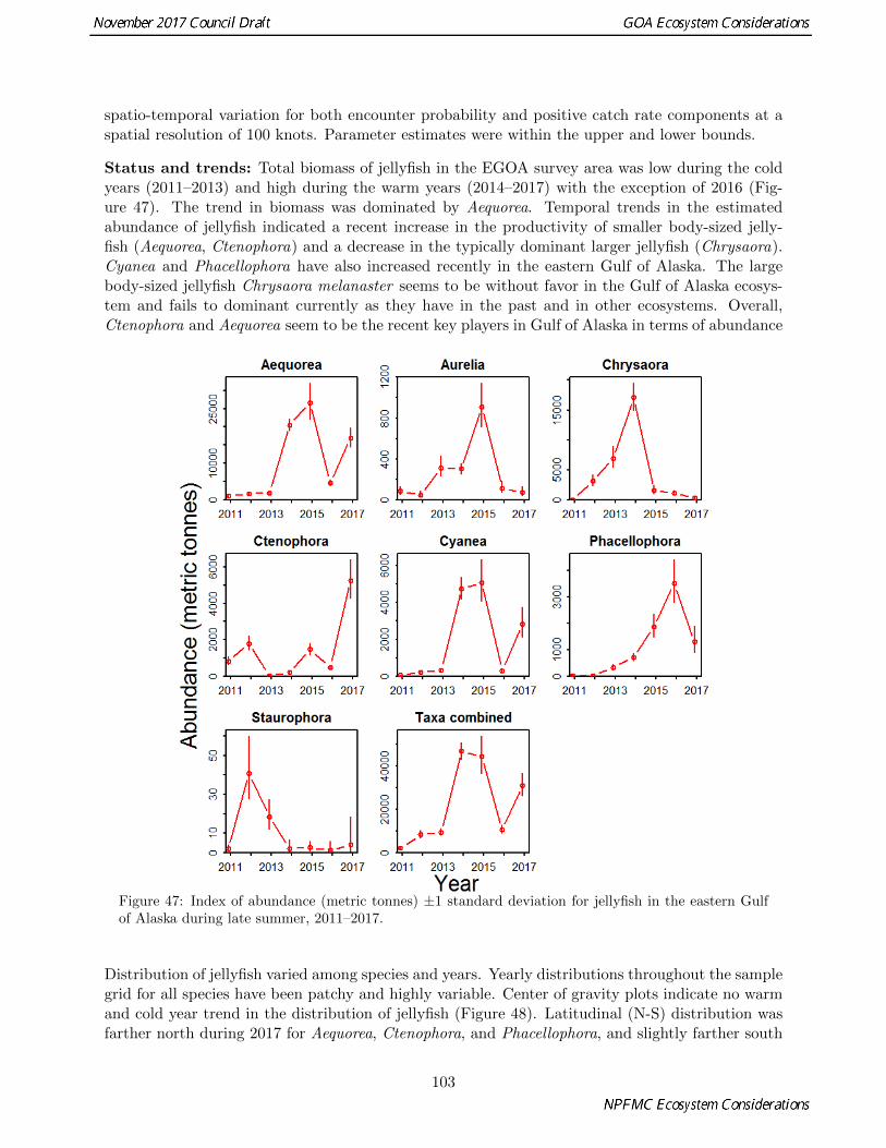
spatio-temporal variation for both encounter probability and positive catch rate components at aspatial resolution of 100 knots. Parameter estimates were within the upper and lower bounds.

Status and trends: Total biomass of jellyfish in the EGOA survey area was low during the coldyears (2011–2013) and high during the warm years (2014–2017) with the exception of 2016 (Fig-ure 47). The trend in biomass was dominated by Aequorea. Temporal trends in the estimatedabundance of jellyfish indicated a recent increase in the productivity of smaller body-sized jelly-fish (Aequorea, Ctenophora) and a decrease in the typically dominant larger jellyfish (Chrysaora).Cyanea and Phacellophora have also increased recently in the eastern Gulf of Alaska. The largebody-sized jellyfish Chrysaora melanaster seems to be without favor in the Gulf of Alaska ecosys-tem and fails to dominant currently as they have in the past and in other ecosystems. Overall,Ctenophora and Aequorea seem to be the recent key players in Gulf of Alaska in terms of abundance

Figure 47: Index of abundance (metric tonnes) ±1 standard deviation for jellyfish in the eastern Gulfof Alaska during late summer, 2011–2017.

Distribution of jellyfish varied among species and years. Yearly distributions throughout the samplegrid for all species have been patchy and highly variable. Center of gravity plots indicate no warmand cold year trend in the distribution of jellyfish (Figure 48). Latitudinal (N-S) distribution wasfarther north during 2017 for Aequorea, Ctenophora, and Phacellophora, and slightly farther south

103

for Aurelia, Chrysaora, and Staurophora, and no different for Cyanea relative to 2016. Longitudi-nal distribution was oriented farther east for Aequorea, Aurelia, Chrysaora, and Staurophora, andfarther west for Ctenophora, Cyanea, and Phacellophora in 2017 relative to 2016. According to theestimated area occupied, the distribution was contracted for Aequorea, Chrysaora, Phacellophora,and Staurophora, and slightly expanded for Aurelia, Ctenophora, and Cyanea during 2017 relativeto 2016 (Figure 49).

Factors influencing observed trends: Shifts in abundance from single-body, large-sized jellyfishduring cold years to multiple, smaller-sized species during warm years indicate that there could bea shift to multiple taxa in the future during warm stanzas. There is not enough eastern Gulf ofAlaska data to determine if this is the trend. The cause for the shifts in biomass and distribution donot seem to rely solely on physical ocean factors (temperature and salinity). These shifts could alsobe a result of environmental forcing earlier in the growing season or during an earlier life historystage (polyp), which may influence large medusae biomasses and abundances (Purcell et al., 2009).The rise in Ctenophore catches could possibly be related to the change in gear but gear effects havenot been determined at this time.

Implications: Significant increases in jellyfish biomass may redirect energy pathways, causing dis-ruption to eastern Gulf of Alaska foodwebs by increased jellyfish predation pressure on zooplanktonand larval fish, which could result in limiting carbon transfer to higher trophic levels (Condon et al.,2011).

104

Figure 48: Center of gravity indicating temporal shifts in the mean east-to-west and north-to-southdistribution plus/minus 1 standard deviation in UTM (km) for jellyfish on the eastern Gulf of Alaskaduring summer, 2011–2017.

105

Figure 49: Effective area occupied (ln(km2)) indicating range expansion/contraction plus/minus 1 stan-dard deviation for jellyfish in the eastern Gulf of Alaska during summer, 2011–2017.

106

Ichthyoplankton

Larval Walleye Pollock Assessment in the Gulf of Alaska, Spring 2017

Contributed by Annette Dougherty and Lauren Rogers, EcoFOCI, Resource Assessment and Con-servation Engineering Division, Alaska Fisheries Science Center, National Marine Fisheries Service,NOAAContact: [email protected] updated: August 2017

Description of indicator: The 2017 EcoFOCI spring larval survey was conducted from May 11to June 2. A total of 267 stations were sampled using the 60 cm bongo with 0.505 mm mesh. Fromthe 60 cm bongos, net 1 was preserved in 1.5% formaldehyde for later identification, quantification,and length measurement of all larval fish species. Net 2 was used to acquire a rough count of larvalpollock while at sea to determine a rough estimate of abundance and geographic distribution.Rough counts were acquired by pouring the codend contents into a 4-liter beaker and removing a10% subsample for sorting. If the larval pollock count was below 10, then the entire codend wassorted. The larval samples removed from net 2 were preserved in alcohol to determine age, growth,hatch date distributions, prey estimates, and condition by cell cycle analysis. The 20/60 bongoarray with 0.153/0.505 mm mesh was used every other survey line to identify and quantify relativezooplankton abundance available for larval fish. A Sea-Bird FastCat was used in conjunction withthe bongos to acquire temperature and salinity profiles. Argos satellite-tracked drifters drogued at40 meters were released east of Kennedy Entrance and between the Semidi Islands and ChirikofIsland (both areas of high larval pollock counts) to assess current strength and direction of larvaltransport.

A time series of larval walleye pollock abundance has been developed using quantitative laboratorycounts of samples from the spring larval survey from 1981–2015 (Rogers and Mier, 2016; Doyleet al., 2009); however, these data are not available until approximately 12 months after the survey.At-sea rough counts of larval walleye pollock provide a rapid indicator of larval abundance, and atime series was constructed for larval rough counts using the same methodology as for laboratory-based counts. Comparison of abundance estimates using at-sea rough counts and laboratory countsfrom 2000–2015 indicate a strong correlation (r = 0.99). At-sea rough counts are only available forwalleye pollock.

Status and trends: Larval walleye pollock rough counts from the 2017 western Gulf of Alaskasurvey were above average throughout the grid with few zero catches (Figure 50). This is in contrastto 2015 when catches were far below average and often zero across the survey grid (Dougherty, 2015).The rough-count abundance estimate indicates that larval walleye pollock abundance was similarto previous high-abundance years (2000, 2006, 2010) although not as high as 2013 (Figure 51).

Factors influencing observed trends: All larval pollock caught were observed to be in excel-lent condition and feeding well. A rapid zooplankton assessment (RZA) was conducted at sea todetermine prey quality and abundance (see Ferm et al., p. 83). Results suggest good conditionsfor pollock larvae and juvenile production. Temperature at 40 meters (larval pollock residence)ranged between 4–6oC, which is closer to the expected temperature range for late May in compari-son to 2015. The Argos satellite-tracked drifter released east of Kennedy Entrance quickly entered

107

Figure 50: At-sea rough counts of larval walleye pollock on the EcoFOCI Spring Survey, DY17-05.Counts are uncorrected for effort.

Shelikof Strait and is currently traveling along the Alaska Peninsula between Sutwik Island andthe Shumagin Islands. The drifter released between Chirikof Island and the Semidi Islands. hastraveled inland to the Alaska Peninsula past the Shumagin Islands and is moving towards PavlofBay. The data from the drifter tracks will be useful to determine if mixing of larval pollock fromgeographically separated spawning stocks is occurring (i.e. Shelikof and Shumagin Islands).

Implications: Observed high abundance of larval walleye pollock indicates good survival throughthe first critical bottleneck period for walleye pollock. This suggests that the ecosystem has returnedto a more productive state after the 2014–2016 warm anomaly. Juvenile walleye pollock are animportant prey species in the Gulf of Alaska. Whether 2017 will be a strong year-class for thewalleye pollock fishery remains to be seen, as high mortality at later stages can reduce even stronglarval and juvenile cohorts, as was seen in 2013.

108

●

●

●

●

●

●

●

●

●

●

● ●

●

●●

● ●

●

● ● ●●

●

●

● ● ●

●

●

●

●

1980 1990 2000 2010

050

015

0025

00

Mea

n ab

unda

nce

(no.

per

10

m2 )

● Laboratory countsAt−sea rough counts

Figure 51: Estimated abundance of larval walleye pollock based on quantitative laboratory-based counts(1981–2015) and at-sea rough counts (2000–2017).

Forage Fish and Squid

Small Neritic Fishes in Coastal Marine Ecosystems: Late-Summer Conditions in theWestern Gulf of Alaska

Contributed by Lauren Rogers, Matthew Wilson, Steven Porter, EcoFOCI Program, Resource As-sessment and Conservation Engineering Division, Alaska Fisheries Science Center, NOAAContact: [email protected] updated: September 2017

Description of indicator: The Ecosystems & Fisheries Oceanography Coordinated Investigations(EcoFOCI) Program monitors and researches small neritic fishes to improve our understanding andmanagement of the Gulf of Alaska ecosystem and fisheries. Small neritic fishes include the juvenilestages of economically and ecologically important species (e.g., walleye pollock, Pacific cod, Pacificocean perch and other rockfishes, sablefish, and arrowtooth flounder). They also include speciesmanaged exclusively as forage fishes (e.g., capelin and eulachon) that support the fishes, seabirds,and marine mammals that characterize the piscivore-dominated GOA ecosystem. Longstandingobjectives of EcoFOCI late-summer field work in the western Gulf of Alaska are to extend a timeseries of age-0 walleye pollock abundance estimates, monitor the neritic environment including

109

zooplankton and abiotic conditions, and collect samples for research (e.g., trophic and spatialecology, bioenergetics, age and growth).

During 21 August–15 September, the NOAA vessel Oscar Dyson sampled the western Gulf of Alaskafrom Cook Inlet to the Shumagin Islands, including Shelikof Strait, the east side of Kodiak Island,and spanning the shelf out to the shelf break. The survey grid west of the Shumagin Islands wastruncated due to weather. At each of 130 stations, water temperature and salinity were profiledand zooplankton samples were collected with 20 cm (153 µm mesh) and 60-cm (505 µm mesh)bongos towed obliquely through the upper 200 m of the water column (see p.83). Target fisheswere collected using a Stauffer trawl (aka anchovy trawl) equipped with a small-mesh (2x3 mm)codend liner towed obliquely to a maximum depth of 200 m.

Time series of abundance for age-0 pollock and for capelin were constructed based on catches fromlate-summer surveys since 2000 (only odd years since 2001) for the consistently sampled regionbetween Kodiak Island and the Shumagin Islands (Figure 52). Mean catch per unit area wascalculated using an area-weighted mean. Due to significant differences in catches of capelin duringday versus night, mean CPUE for the night stations only is also shown.

●

●●

●

●

●

●●

●

●

●

●

●

●

●

●

●●

●

●

●

●

●

●

●●●

●

●

●

●●

●

●

● ●

●●

●

●

●

●●

●

●

●

●

●

●

● ●

●

●

●

●

●

●

●●

●●

●

●

●

●

●●●●

●

●

●

●

●

●

●

●

●

●

●

●

●

●

●

●

● ●

●

●

●●●●●●

●

●● ●

●●●●

●●●

●●●

●●●

●●●

●

●

●

●

●

●●

●

●

●●●

●

●

●

●●●●

●●

●●

●

●

●

●●

●

●●

● ●●

●

●

●

●●

●

●

●

●

●

●

●

●

●●

●

●

●

●

● ●

2013

−165 −160 −155 −150

5456

5860

●

●

●●

●

● ● ●

●

●

●

●●

●

●

●

●

●

●

●

●

●

●

●

●

●

●

●

●

●●

●

●

●

●

●

●●

●

●

●

●

●

●●

●

●

●

●

●

●

●●

●

●

●

●

●

●

●

●●

●

●

●

●

●

● ●

2015

−165 −160 −155 −150

5456

5860

●●

●

●

●●●

●

●

●

●●●●●●

●●

●●●●●●

●●●●●● ●

● ●●

●●●

●●●● ●

●

●

●

●●

● ●

●●●●●●● ●

●●

●●

●

●

●●

●●●

●●

●●

●

●

●●

●●

●●

●

●

●

●●● ●

● ●

●●

●

●

●

●

●

●●●

●

●●

●

●

●

●

●●

●

●

●

●

2017

−165 −160 −155 −150

5456

5860

●

●

●

Age−0 Pollock (No per m2)

00.050.55

Figure 52: Catches of age-0 walleye pollock in the EcoFOCI late-summer small-mesh trawl survey for2013, 2015, and 2017. The area in the blue dashed box indicates the region most consistently sampledsince 2000 and includes the stations used to develop CPUE time series.

Status and trends: Catches of age-0 pollock were particularly high through Shelikof Strait and tothe east of Kodiak Island (Figure 52). The mean CPUE estimate for 2017, which does not includethe stations near Kodiak, suggests the second highest abundance of age-0 pollock in our time series

110

(Figure 53), averaging 380,000 age-0 pollock per square kilometer (0.38 fish/m2). Pollock densitiestapered off towards the Shumagin Islands in the southwest. This spatial distribution is in contrastto a previous high abundance year (2013) when catches were highest southwest of the ShumaginIslands. Capelin abundance remained low in 2017, continuing a trend of low abundance since 2011.However, note that no sampling occurred in even years and the time series estimate does not includecatches from near Kodiak, where capelin catches are typically higher.

● ● ●

●

●

● ●

●

●

●

2000 2005 2010 2015

0.0

0.2

0.4

0.6

0.8

Age 0 Pollock

Age

−0

Mea

n C

PU

E (N

om

2 )

(A)

040

080

012

00

Age

−1

(MA

CE

She

likof

)

020

0040

0060

00

Age

−1

(Ass

essm

ent m

odel

)

● EcoFOCI Age−0Age−1 (MACE Shelikof)Age−1 (Assessment)

● ● ●

●

●

●● ● ● ●

2000 2005 2010 2015

0.0

0.2

0.4

0.6

0.8

1.0

Capelin

Mea

n C

PU

E (N

om

2 ) ● Day & NightNight only

(B)

Figure 53: Catches of age-0 walleye pollock in the EcoFOCI late-summer small-mesh trawl survey for2013, 2015, and 2017. The area in the blue dashed box indicates the region most consistently sampledsince 2000 and includes the stations used to develop CPUE time series.

Factors influencing observed trends: The abundance of age-0 pollock in late summer reflectsthe number of surviving larvae from spawning in the spring and survival processes through thesummer. In spring of 2017, catches of larval pollock were high (Dougherty and Rogers, p.107), anda rapid assessment of zooplankton in late summer (Ferm et al., p.83) suggested high abundanceof euphausiids and large copepods, preferred prey for pollock. The observed spatial distributionof pollock may result from transport processes and/or reflect production from different spawninggroups. Investigations into factors driving changes in the spatial distribution and abundance ofcapelin and juvenile pollock are underway.

Implications: Capelin and young-of-year pollock are key forage fish species in the Gulf of Alaska,providing prey for seabirds, fishes, and mammals. This late-summer survey also provides an as-

111

sessment of the abundance, size, and condition of young-of-year pollock before entering their firstwinter, giving an early indicator of potential year class strength. Strong catches of juvenile pollock,together with previously observed high larval abundance, suggest a return to productive conditionsin the Gulf of Alaska following the “Blob” warm anomaly in 2014–2016.

Capelin and Sand Lance Indicators for the Gulf of Alaska

Contributed by Stephani Zador and Madisyn FrandsenResource Ecology and Fishery Management Division, Alaska Fisheries Science Center, NationalMarine Fisheries Service, NOAAContact: [email protected] updated: August 2016This will be updated in 2018.

Seabird-Derived Forage Fish Indicators from Middleton Island

Contributed by Scott A. Hatch1, Mayumi Arimitsu2, John F. Piatt21 Institute for Seabird Research and Conservation, Anchorage, AK2 Seabird and Forage Fish Ecology Program, Marine Ecosystems Office, Alaska Science Center U.S.Geological Survey, Anchorage, AKContact: [email protected] updated: August 2017

Description of indicator: Time series of seabird and forage fish monitoring at Middleton Islandin the north-central Gulf of Alaska are among the longest available from any Alaska location. Beingsituated near the continental shelf edge (lat 59.4375, lon -146.3277), Middletons seabirds sampleboth neritic habitat and deep ocean waters beyond the shelf break. Consequently, certain species ofecological concern (myctophids) and/or economic concern (0-age group sablefish) figure prominentlyin seabird diets at Middleton, unlike anywhere else these prey and their seabird predators mightbe monitored.

In most years since 2000, regurgitated food samples have been collected from adult and/or nestlingblack-legged kittiwakes (Rissa tridactyla) during all months April through August. From an evalua-tion of alternate methods of analyzing and reporting diet results, the preferred metric for kittiwakesis prey relative occurrence (Hatch, 2013), for which the relevant sample units are numbers of identi-fied prey types in a given sample. Rhinoceros auklet (Cerorhinca monocerata) diets are monitoredby collecting bill-loads from chick-provisioning adults, usually once or twice a week from early Julythrough early or mid-August. Since 1978, more than 100 kg of auklet prey samples have beencollected on Middleton, and auklet diet monitoring provides our single best indicator of forage fishdynamics in the region.

Status and trends: On average, Middleton kittiwakes take about equal amounts of Pacific sandlance, capelin, and invertebrates, with lesser amounts of herring, sablefish, salmon, and myctophids,depending on stage of the season. The juxtaposition of time series for kittiwakes and rhinocerosauklets since 1978 (Figure 54) shows general agreement between a sustained decline of sand lanceand, beginning in 2007, the emergence of capelin as a dominant forage species. In the last 4 years,

112

however, when neither sand lance nor capelin were prevalent, the diets of surface-feeding kittiwakesand diving auklets diverged in respect to prey-switching to alternate species such as mytophids andsalmon.

Auklet data plotted separately by prey type highlight the interannual dynamics of individual species(Figure 55). By all appearances, sand lance were the overwhelmingly dominant forage species in thenorthern Gulf in the late 1970s through the early 1980s. Following a period of reduced availabilityin the mid 1990s, sand lance made a strong comeback by the end of that decade. However, sandlance steadily declined in importance after 2000 and for the most part have contributed little toseabird diets since 2008. However, the appearance of about 30% sand lance in the auklet diet in2016 and 2017 is consistent with a known association of sand lance with warm-water conditions(Hatch, 2013). Pacific herring seem also to have benefited from recent warm surface conditionsprevalent in the region

Factors influencing observed trends: Seabird diets at Middleton reflect ecosystem shifts inthe Gulf of Alaska. This includes specific events recorded and widely discussed in the ecologicalliterature such as the notable shift from “warm” (positive Pacific Decadal Oscillation, PDO) con-ditions to cold (negative PDO) conditions around 1999–2000 (Greene, 2002; Peterson et al., 2003;Batten and Welch, 2004), a similar but stronger and more persistent shift in 2008 (Hatch, 2013),and a widely reported warm-water anomaly that has dominated the system since late winter 2013(Bond et al., 2015)). A salient finding during a recent, anomalous warm-water event has been thevirtual disappearance of capelin from the kittiwake diet on Middleton, following 6 prior years whencapelin were predominant (Figure 54). An apparent trade-off between Pacific sand lance (warmconditions) and capelin (cold conditions) may be a benchmark of the forage fish community in theregion.

Implications: Seabird diets provide further evidence that capelin disappeared in the ecosystemduring the recent warm years. Chick diets at Middleton may be informative for sablefish studies.In 2017, the Alaska Fisheries Science Center will begin using specimens from seabird diet samplingat Middleton for phenology and growth studies of first-year sablefish, which are difficult to sampledirectly. Seabird diet indicators are potentially applicable to other management concerns in theregion, including Pacific herring stocks, which crashed and have not recovered after the Exxon-Valdez Oil Spill in 1989, and year-class strengths of pink and chum salmon, which appear regularlyin Middleton seabird diets.

113

3

Fig. 1. Interannual variation in diet composition of chick-rearing rhinoceros auklets on Middleton Island, 1978 to 2017, with a similar time series for black-legged kittiwakes (lower panel) for comparison.

0.0

0.2

0.4

0.6

0.8

1.0Pr

opor

tion

of b

iom

ass

Year

RHAU chick diet

Sand lance Capelin Salmon Sablefish Greenling Herring

0.0

0.2

0.4

0.6

0.8

1.0

Rela

tive

occu

rren

ce

Year

Kittiwake June-August

Sand lance Capelin Herring SablefishMyctophids Salmon Other fish Invertebrates

Figure 54: Interannual variation in diet composition of chick-rearing rhinoceros auklets on MiddletonIsland, 1978–2017, with a similar time series for black-legged kittiwakes (lower panel) for comparison.

114

4

Fig. 2. Indices of prey species occurrence in the nestling diet of rhinoceros auklets on Middleton Island from 1978 through 2017.

Prop

ortio

n of

bio

mas

s

Year

0.0

0.1

0.2

0.3

0.4 Pacific herring

0.00.20.40.60.81.0

Sand lance

0.00.10.20.30.40.50.6

Capelin

0.00.10.20.30.40.50.6

Pink & chum salmon

0.00.10.20.30.40.5 Y-O-Y Sablefish

Figure 55: Prey species occurrence in the nestling diet of rhinoceros auklets on Middleton Island from1978–2017.

115

Spatial and temporal trends in the abundance and distribution of YOY groundfish inpelagic waters of the eastern Gulf of Alaska during summer, 2010–2017

Contributed by Wes Strasburger, Jamal H. Moss and Ellen Yasumiishi, Auke Bay LaboratoriesDivision, Alaska Fisheries Science Center, National Marine Fisheries Service, NOAAContact: [email protected] updated: October 2017

Description of indicator: Pelagic fish were sampled using a rope trawl towed in the upper 20m during the Alaska Fisheries Science Center’s eastern Gulf of Alaska Assessment Survey, summer2010–2017. Stations were approximately 10 nautical miles apart and hauls were standardized toapproximately 30 minutes. Area swept was estimated from horizontal net opening and distancetowed. The Nordic 264 trawl was used in 2010 and 2017, and a CanTrawl 400/601 was used in2011–2016.

Fish catch was estimated in kilograms. Young-of-the-year (YOY) marine fish weight was esti-mated by multiplying the grand mean weight in a given year by the number captured at a station.Four YOY groundfish species were captured in the trawl, including: Pacific cod, walleye pollock,arrowtooth flounder, and rockfish (Sebastes spp.).

Abundance and distribution (center of gravity and area occupied) were estimated using the VASTpackage for multispecies version 1.1.0 (Thorson et al., 2015; Thorson and Kristensen, 2016; Thorsonet al., 2016a,b). This package generates a standardized geostatistical index, used for estimatingabundance for stock assessments. We specified a gamma distribution and estimated spatial andspatio-temporal variation for both encounter probability and positive catch rate components at aspatial resolution of 100 knots (100 prediction units). Parameter estimates were within the upperand lower bounds and final gradients were less than 0.0005. If no positive catches occurred fora species within a year, an artificial minimum value was inserted, allowing the model to run. Itis important to note that no YOY Pacific cod were sampled in 2016. This resulted in very largeconfidence intervals on a low point. The overall trend is still what would be expected.

Status and trends: YOY biomass estimates indicate high levels of arrowtooth flounder, and lowlevels of Pacific cod, pollock, and rockfish in 2017. Temporal trends in the estimated abundance ofthese groundfish species indicated above average abundance of arrowtooth flounder in 2012, aboveaverage abundance of Pacific cod in 2014, above average abundance of pollock during 2014, and anabove average abundance of rockfish in 2016 (Figure 1). In 2016, rockfish were the most abundantYOY marine fish species in 2016 followed by pollock, and arrowtooth flounder (Figure 56).

Distribution of groundfish in pelagic waters varied among species and years. Pacific cod werecommonly predicted to be over the shelf (50–200 m bottom depth) and within 20 nm from shore.Pollock were more widely distributed, occupying shelf, slope, and basin domains (50–2000 m bottomdepth). Rockfish were the most widely distributed species in the eastern Gulf of Alaska; occupyingshelf, slope, and basin domains up to 100 nm from shore. Arrowtooth flounder were typically foundoffshore, with the exception of in 2012. In 2017, Pacific cod were found off of Yakutat Bay andBaranof Island, pollock were found north and offshore, arrowtooth flounder in the northern regionof the survey area, and rockfish fairly evenly distributed across the shelf.

Center of gravity indicated that all species were distributed farther north in 2017. Pacific cod

116

Figure 56: Index of abundance (metric tonnes) plus/minus 1 standard deviation for groundfish speciesin pelagic waters of the eastern Gulf of Alaska during summer, 2010–2017.

were distributed farther north during recent warm years (2014–2015), whereas pollock, arrowtoothflounder, and rockfish were not until 2017 (Figure 2). Range expansion or contraction occurred forall species in 2017 relative to 2016, except for pollock (Figure 3).

Factors influencing observed trends: Lower groundfish abundances in pelagic waters during2017 are believed to be in response to poor primary production (Strom et al., 2016) and an increasedabundance of salps (Li et al., 2016), which further reduced the amount of plankton available transferenergy to upper trophic levels. Piscivorous predators not common to the eastern Gulf of Alaska(e.g., Pacific pomfret) were present in the eastern Gulf of Alaska during 2014, and 2015, presumablyin response to unprecedented warming in the eastern Pacific Ocean commonly referred to as the“Warm Blob” (Bond et al., 2015). Additional predation pressure by these warm water predatorsmay have reduced the amount of YOY marine fish that would have otherwise been present.

Implications: Lower groundfish abundances in surface waters during 2017 indicate a change inproductivity in pelagic waters that affected many species of YOY marine fish. Warm conditionsduring 2014 and 2015 appeared to initially benefit pollock and Pacific cod and in more recent yearsbenefited arrowtooth flounder and rockfish. No Pacific cod were sampled during 2016. Additionally,Pacific cod were low for 2010–2013 year classes in the survey area, a period of cool temperatures.

117

Figure 57: Center of gravity indicating temporal shifts in the mean east-to-west and north-to-southdistribution plus/minus 1 standard deviation in UTM (km) for groundfish in pelagic waters of theeastern Gulf of Alaska during summer, 2010–2017.

118

Figure 58: Effective area occupied (ln(km2)) indicating range expansion/contraction plus/minus 1 stan-dard deviation for groundfish in pelagic waters of the eastern Gulf of Alaska during summer, 2010–2017.

119

Spatial and Temporal Trends in the Abundance and Distribution of Juvenile PacificSalmon in the Eastern Gulf of Alaska during Summer 2011–2017

Contributed by Jamal Moss, Wesley Strasburger, and Ellen Yasumiishi, Auke Bay LaboratoriesDivision, Alaska Fisheries Science Center, National Marine Fisheries Service, NOAAContact: [email protected] updated: October 2017

Description of indicator: Pelagic fish were sampled using a trawl net towed in the upper 20 mof the eastern Gulf of Alaska (EGOA) during the Alaska Fisheries Science Centers Gulf of AlaskaAssessment Surveys during summer, 2010–2017. Stations were approximately 10 nautical milesapart and a trawl was towed for approximately 30 minutes. The area swept by the trawl wasestimated from horizontal net opening and distance towed. Fish catch was estimated in kilograms.Juvenile salmon weight was estimated by multiplying the grand mean weight in a given year by thenumber captured at a station. A CanTrawl was used to sample fish during 2011–2016 and Nordictrawl was used to sample fish in 2017.

Abundance and distribution (center of gravity and area occupied) were estimated for juvenileChinook (Oncorhynchus tshawytscha), chum (O. keta), pink (O. gorbuscha), and sockeye (O. nerka)salmon using the VAST package for multispecies version 1.1.0 (Thorson et al., 2015; Thorson andKristensen, 2016; Thorson et al., 2016a,b) in RStudio version 1.0.136 and R software version 3.3.0(R Core Team 2016). The abundance index is a standardized geostatistical index developed byThorson et al. (2015); Thorson and Kristensen (2016); Thorson et al. (2016a,b) to estimate indicesof abundance for stock assessments. We specified a gamma distribution and estimated spatial andspatio-temporal variation for both encounter probability and positive catch rate components at aspatial resolution of 100 knots. Parameter estimates were within the upper and lower bounds andfinal gradients were less than 0.0005.

Status and trends: Temporal trends in the estimated biomass of juvenile salmon in the EGOAshelf survey area indicates a decrease in the productivity of juvenile salmon during 2017 (Figure 59).Abundances were low for Chinook, coho, pink, and sockeye salmon, and moderate for chum salmon.Both juvenile pink and chum salmon had an alternating year pattern with higher abundances ineven-numbered years. Juvenile salmon were distributed nearshore in waters above the continentalshelf. Juvenile salmon were distributed farther south and east in 2017 relative to 2016 (Figure 59).In 2017, area occupied was contracted for Chinook, coho, and sockeye, and expanded for pink andchum salmon (Figure 59).

Factors influencing observed trends: Lower abundances of juvenile salmon during 2017 waslikely due to a combination of lower odd-brood year pink salmon production and due to the con-tinuation of warm waters and low and patchy ocean productivity.

Implications: Recent decreases in the abundance of juvenile salmon in our survey area duringsummer implies a decline in conditions for growth and survival of salmon from southeast Alaska,British Columbia and the Pacific Northwest lakes and rivers and/or a change in the distribution ofjuvenile salmon into our survey area during July. The size of juvenile salmon in the surveys werealso observed as smaller than usual. Juvenile indices may be an early indication for the numbersof returning adults to the region of origin.

120

Figure 59: Index of abundance (metric tonnes) plus/minus 1 standard deviation for Pacific salmon inthe eastern Gulf of Alaska during late summer, 2010–2017.

121

Figure 60: Center of gravity indicating temporal shifts in the mean east-to-west and north-to-southdistribution plus/minus 1 standard deviation in UTM (km) for juvenile Pacific salmon on the easternGulf of Alaska during late summer, 2010–2017.

122

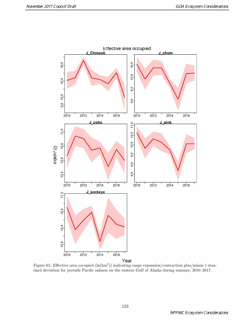
Figure 61: Effective area occupied (ln(km2)) indicating range expansion/contraction plus/minus 1 stan-dard deviation for juvenile Pacific salmon on the eastern Gulf of Alaska during summer, 2010–2017.

123

Spatial and Temporal Trends in the Abundance and Distribution of Squid in theEastern Gulf of Alaska during Summer 2011–2017

Contributed by Jamal Moss, Wesley Strasburger, and Ellen Yasumiishi, Auke Bay LaboratoriesDivision, Alaska Fisheries Science Center, National Marine Fisheries Service, NOAAContact: [email protected] updated: October 2017

Description of indicator: Squid were sampled using a trawl net towed in the upper 20 m ofthe eastern Gulf of Alaska (EGOA) during the Alaska Fisheries Science Center’s Gulf of AlaskaAssessment Surveys during summer, 2011–2017. Stations were approximately 10 nautical milesapart and a trawl was towed for approximately 30 minutes at each station. A CanTrawl was usedfrom 2011–2016 and a Nordic trawl in 2017. The area swept by the trawl was estimated fromhorizontal net opening and distance towed. Squid catch was estimated in kilograms by year andstation. Squid weight at each station was estimated by multiplying the grand mean weight in agiven year by the number captured at a station.

Abundance and distribution (center of gravity and area occupied) were estimated using the VASTpackage for multispecies version 1.1.0 (Thorson et al., 2015; Thorson and Kristensen, 2016; Thorsonet al., 2016a,b) in RStudio version 1.0.136 and R software version 3.3.0 (R Core Team 2016). Theabundance index is a standardized geostatistical index developed by Thorson et al. (2015, 2016a)to estimate indices of abundance for stock assessments. We specified a gamma distribution andestimated spatial and spatio-temporal variation for both encounter probability and positive catchrate components at a spatial resolution of 100 knots. Parameter estimates were within the upperand lower bounds and final gradients were less than 0.0005.

Status and trends: Squid were most abundant in the EGOA during 2014 (Figure 62). Temporaltrends in squid abundances indicate that squid has steadily increased since 2011 with the exceptionof a large spike in abundance in 2014 and slight decline in 2017. Squid were distributed across theshelf but farther offshore during 2011–2015 and nearshore during 2016 and 2017 (Figure 63). Squidwere distributed farther northwest during 2017 relative to 2016. During the 2014–2017 warm years,squid were generally distributed farther north relative to the prior cold years 2011–2013 (Figure64). The area that squid occupied in the survey area declined over the 2011–2017 year period(Figure 65).

Factors influencing observed trends: Squid abundance was lowest during 2011 and may becorrelated with poor primary production. Abundances of squid in the EGOA during 2014 mayhave been in response to unprecedented warming in the eastern Pacific Ocean and influx of thewater mass referred to as the “Warm Blob” (Bond et al., 2015).

Implications: Predators not common to the eastern Gulf of Alaska were present in the EGOAduring 2014, and 2015, presumably in response to the “Warm Blob” (Bond et al. 2015). Wespeculate that forage such as squid may have attracted predators to the EGOA shelf. Squid is ahigh energy prey item for marine species. The high abundances of squid in 2014 may had increasedthe quality and quantity of prey for predators and subsequent survival for species such as salmon.Good feeding conditions during the early marine and pre- and post-winter life stages of juvenilesalmon is thought to improve body condition and survival of salmon to adulthood. The highabundances of squid in 2014 corresponded with the 2014 juvenile year for salmon that had higher

124

Figure 62: Index of abundance (metric tonnes) plus/minus 1 standard deviation for squid in the easternGulf of Alaska during late summer, 2011–2017.

returns of chum salmon (that typically mature after 3 winters in the ocean) to Alaska in 2017 andhigh returns of pink salmon (that mature after one winter in the ocean) to Alaska in 2015.

125

Figure 63: Predicted field densities of squid in the eastern Gulf of Alaska during summer, 2011–2017.

Figure 64: Center of gravity indicating temporal shifts in the mean east-to-west and north-to-southdistribution plus/minus 1 standard deviation in UTM (km) for squid in the eastern Gulf of Alaskaduring summer, 2011–2017.

Figure 65: Effective area occupied (ln(km2)) indicating range expansion/contraction plus/minus 1 stan-dard deviation for squid on the eastern Gulf of Alaska during summer, 2011–2017.

126

Herring

Southeastern Alaska Herring

Contributed by Kyle Hebert and Sherri Dressel, Alaska Department of Fish and Game, CommericalFisheries Division, P. O. Box 110024, Juneau, AK 99811-0024Contact: [email protected] updated: July 2017

Description of indicator: Pacific herring (Clupea pallasi) stocks that reside in southeasternAlaskan waters are defined on a spawning area basis. In recent decades there have been about ninespawning areas where spawning events have typically been annual and meaningful in size relativeto potential for commercial exploitation. These areas include Sitka Sound, Craig, Seymour Canal,Hoonah Sound Hobart Bay-Port Houghton, Tenakee Inlet, Ernest Sound, West Behm Canal, andKah Shakes-Cat Island (Figure 66). Stock assessments have been conducted at these areas formost years since at least the 1980s by the Alaska Department of Fish and Game, primarily throughmodeling that relies on indices of egg deposition, age, and size (Hebert, 2017). Although spawningat these areas accounts for a large proportion of the spawning biomass in southeastern Alaskain any given year, other areas with more limited spawning also exist throughout southeasternAlaska. However, little or no stock assessment activity occurs at these minor locations other thanoccasional and opportunistic aerial surveys to document the miles of spawn along shoreline. Theherring that spawn in all areas of Southeast Alaska are believed to be affected by the physical andchemical characteristics of Gulf of Alaska waters, though the spawning areas directly exposed tothe open coast (Sitka Sound, Craig, Kah Shakes-Cat Island) may be affected the greatest or themost immediately.

Status and trends: Since peaking around the early 2010s, several stocks have decreased substan-tially. The current biomass level for Southeast Alaskan herring in aggregate is below the mean levelover the base period 2009–2016 (Figure 67). This also holds true for every individual stock in theregion. Biomass levels prior to the base period were also below the mean level of the base period,for both combined biomass and for most years of individual stocks. Biomass levels, both currentand historical, are low relative to the base period because the base period partially coincides withthe most productive period for herring in Southeast Alaska that has been documented since atleast 1980. Although the two largest and most consistent stocks (Sitka Sound and Craig), havedeclined substantially from their peaks around 2011, they continue to be at levels above the thresh-olds necessary to allow commercial fisheries. Other, smaller stocks in the region have declined tomuch lower levels over the past few years and in some cases to small fractions of their peaks a fewyears ago (e.g., Hoonah Sound, Seymour Canal, Ernest Sound). Age-structured stock assessmentmodeling indicates that the decline can be attributed at least in part to lower survival rates overthe past few years.

Factors influencing observed trends: The underlying cause for the recent decline in herringsurvival and biomass in the region remains unknown. Multiple plausible factors may be contribut-ing, including increasing populations of predatory marine mammals, such as humpback whales andStellar sea lions (Sigler et al., 2009; Muto et al.; Fritz et al., 2016), high levels of predatory fishsuch as salmon, or the recent shift to warmer sea surface temperatures as reflected in the PDO,which could affect herring prey or metabolism.

127

Figure 66: Location of nine important Pacific herring spawning locations in Southeast Alaska..

Implications: Although it is possible that lower abundance of herring in the region may haveshort-term deleterious effects on predators that rely on herring, there is not enough informationabout populations of other forage species to understand the broader net impact on predators. Theshort life-span of herring and the natural volatility of stock levels, particularly of smaller-sizedstocks, make it difficult to speculate on long-term implications to the ecosystem.

128

0

50,000

100,000

150,000

200,000

250,000

300,000

1980198219841986198819901992199419961998200020022004200620082010201220142016

Estim

ated m

ature

bioma

ss (to

ns)

Year

Total SEAK biomassSEAK biomass, minus SitkaSitka biomassAverage 2009-2016 total SEAK

Figure 2. Estimated combined annual mature herring biomass (prefishery, including and excluding Sitka) at nine important southeastern Alaska spawning areas, 1980-2016. Black line indicates average of combined Southeast Alaska herring biomass during base period of 2009-2016.

Figure 67: Estimated combined annual mature herring biomass (prefishery, including and excludingSitka) at nine important southeastern Alaska spawning areas, 1980–2016. Black line indicates averageof combined Southeast Alaska herring biomass during base period of 2009–2016.

129

Salmon

Salmon Trends in the Southeast Coastal Monitoring (SECM) Survey

Contributed by Jordan T. Watson, Andy Gray, Emily Fergusson, James M. Murphy, Auke BayLaboratories Division, Alaska Fisheries Science Center, National Marine Fisheries Service, NOAAContact: [email protected] updated: August 2017

Description of indicator: The Southeast Coastal Monitoring (SECM) program has collected fish,zooplankton, and oceanographic samples in southeast Alaska since 1997 (Fergusson et al., 2013;Orsi et al., 2014, 2015). Sampling has been focused most consistently in Icy Strait, the primarynorthern migratory pathway to the Gulf of Alaska for juvenile salmon originating from over 2000southeast Alaska streams and rivers. Research objectives of the SECM program are to provideinsight into the production dynamics and early ocean ecology of Southeast Alaska salmon.

Surface trawls (0–20m) are used to sample epipelagic fish species, including all five commercialspecies of Pacific salmon (Oncorhynchus sp.) in southeast Alaska. Juvenile pink salmon (O.gorbuscha) are, on average, the most abundant species in the epipelagic habitat in SECM surveys.In addition to juvenile salmon, SECM surveys catch a suite of non-salmonid fish species, includingoccasional large numbers of walleye pollock (Gadus chalcogrammus), capelin (Mallotus villosus),and Pacific herring (Clupea pallasii). We provide summaries of the annual catch rates for thefive salmon species (pink; coho O. kisutch; sockeye, O. nerka; chum, O. keta; and Chinook, O.tshawytscha).

Status and trends: In 2017, juvenile salmon catch rates were among the lowest of the time seriesfor all five salmon species (Figure 68). Meanwhile, adult chum salmon catch rates continued anupward trend, though these rates remain nearly an order of magnitude lower than those of adultpink salmon.

Factors influencing observed trends: Ocean conditions in 2017 were preceded by severalanomalously warm years. Warm ocean conditions are likely to have influenced recruitment patternsthrough multiple years of altered community structure and stock dynamics. We continue to seekrelationships between observed trends and environmental covariates (e.g., sea surface temperature).

Implications: Understanding recruitment processes of fish stocks is an important aspect of man-aging fish stocks, particularly during periods of substantial climate change. Juvenile abundanceand oceanographic data collected during SECM have provided reliable forecasts of pink salmonreturns to Southeast Alaska (Orsi et al., 2015) and are used for pre-season fisheries managementdecisions in the purse seine and drift gillnet fisheries of Southeast Alaska (Wertheimer et al., 2015).By extending the application of SECM fish catches beyond pink salmon, we are poised to betterresolve the relationships between other salmon species and ecosystem indicators that help to de-scribe their production dynamics. Furthermore, as SECM surveys continue annually, they fill avaluable gap in data that occurs during off-years for the Gulf of Alaska Ecosystem Surveys.

130

Figure 68: Time series of juvenile, immature (Chinook only), and adult salmon catch rates (number offish per hour) during SECM surveys from 1997–2017.

Marine Survival Index for Pink Salmon from Auke Creek, Southeast Alaska

Contributed by Scott C. Vulstek, Joshua R. RussellAuke Bay Laboratories Division, Alaska Fisheries Science Center, National Marine Fisheries Ser-vice, NOAAContact: [email protected] updated: September 2017

Description of indicator: The 1980–2016 time series of marine survival estimates for wild pinksalmon from the Auke Creek Research Station in Southeast Alaska is the longest-running continuousseries available in the North Pacific. The Auke Creek weir structure facilitates near-completecapture of all migrating pink fry and returning adults, and is the only weir capable of such on a wildsystem in the North Pacific. Marine survival is estimated as the number of adults (escapement) perfry. The index is presented by fry outmigration year. While no stock-specific harvest informationis available for Auke Creek pink salmon, and there are possible influences of straying and intertidalproduction downstream of the weir structure, the precision of this long-term dataset makes it anexcellent choice for model input relating to nearshore and gulf-wide productivity.

131

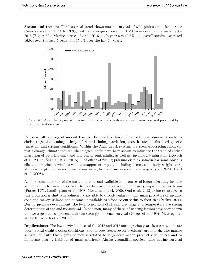
Status and trends: The historical trend shows marine survival of wild pink salmon from AukeCreek varies from 1.2% to 53.3%, with an average survival of 11.2% from ocean entry years 1980–2016 (Figure 69). Marine survival for the 2016 smolt year was 10.6% and overall survival averaged16.9% over the last 5 years and 15.4% over the last 10 years.

Figure 69: Auke Creek pink salmon marine survival indices showing total marine survival presented byfry outmigration year.

Factors influencing observed trends: Factors that have influenced these observed trends in-clude: migration timing, fishery effort and timing, predation, growth rates, maintained geneticvariation, and stream conditions. Within the Auke Creek system, a system undergoing rapid cli-matic change, climate-induced phenological shifts have been shown to influence the trend of earliermigration of both the early and late run of pink adults, as well as, juvenile fry migration (Kovachet al. 2013b, Shanley et al. 2015). The effect of fishing pressure on pink salmon has some obviouseffects on marine survival as well as unapparent impacts including decreases in body weight, vari-ations in length, increases in earlier-maturing fish, and increases in heterozygosity at PGM (Hardet al. 2008).

As pink salmon are one of the most numerous and available food sources of larger migrating juvenilesalmon and other marine species, their early marine survival can be heavily impacted by predation(Parker 1971, Landingham et al. 1998, Mortensen et al. 2000, Orsi et al. 2013). One resistance tothis predation is that pink salmon fry are able to quickly outgrow their main predators of juvenilecoho and sockeye salmon and become unavailable as a food resource due to their size (Parker 1971).During juvenile development, the local conditions of stream discharge and temperature are strongdeterminants of egg and fry survival. In addition, many of these influencing factors have been shownto have a genetic component that can strongly influence survival (Geiger et al. 1997, McGregor etal. 1998, Kovach et al. 2013a).

Implications: The low survival indices of the 2015 and 2016 outmigration year classes may indicatepoor habitat quality, ocean conditions, and/or prey resources for predatory groundfish. The marinesurvival of Auke Creek pink salmon is related to large-scale ocean productivity indices and toimportant rearing habitats of many southeast Alaska groundfish species. The marine survival

132

of indices of Auke Creek pink salmon provide trends that allow for the examination of annualvariation in habitat quality of rearing areas and general ocean conditions and productivity. Dueto the one ocean year life history of pink salmon, we are able to use their marine survival as aproxy for the general state of the Gulf of Alaska. Additionally, as pink fry are such a numerousfood resource in southeast Alaska, their abundance and rate of predation allow for insights intothe groundfish fisheries. Pink fry have been shown to be an important food resource for juvenilesablefish, making up a large percentage of their diet (Sturdevant et al. 2009, 2012). The growthand marine survival of Auke Creek pink salmon provide valuable proxies for Gulf of Alaska andsoutheast Alaska productivity, as well as, the overwintering survival and recruitment of sablefish.

Marine Survival Index for Coho Salmon from Auke Creek, Southeast Alaska

Contributed by Scott C. Vulstek, Joshua R. Russell, Ellen M. YasumiishiAuke Bay Laboratories Division, Alaska Fisheries Science Center, National Marine Fisheries Ser-vice, NOAAContact: [email protected] updated: September 2017

Description of indicator: The time series of marine survival estimates for wild coho salmon fromthe Auke Creek Weir in Southeast Alaska is the most precise and longest-running continuous seriesavailable in the North Pacific. Auke Bay Laboratories began monitoring wild coho salmon survivalin 1980. All coho salmon smolts leaving the Auke Lake watershed have been counted, subsampledfor age and length, and injected with coded wire tags (CWT). Research studies over the last 36years have captured and sampled virtually all migrating wild juvenile and adult coho salmon. Thesemigrating fish included those with both 1 and 2 freshwater annuli and 0 or 1 ocean annuli. Marinesurvival is estimated as the number of adults (harvest plus escapement) per smolt. The indexis presented by smolt (outmigration) year. The precision of the survival estimate was high dueto 100% marking and sampling fractions that minimized the variance in the survival estimate andmade the series an excellent choice for model input relating to nearshore and gulf-wide productivity.It is the only continuous marine survival and scale data set in the North Pacific that recovers allreturning age classes of wild, CWT coho salmon as ocean age 0 and 1

Status and trends: The historical trend shows marine survival of wild coho salmon from AukeCreek varies from 5.1% to 47.8%, with an average survival of 23.7% from smolt years 1980–2015(Figure 70; top panel). Marine survival for 2015 was the lowest on record at 5.1% and overallsurvival averaged 16.2% over the last 5 years and 17.9% over the last 10 years. The survival indexfor ocean age-1 coho varies from 3.9% to 36.6% from smolt years 1980–2015 (Figure 70; middlepanel) and for ocean age-0 coho varies from 1.1% to 11.2% from smolt years 1980–2016, with 2015being the lowest on record (Figure 70; bottom panel). Return data for 2017 returns are included,despite the fact that the run is not completely finished. These data are included because the marinesurvival for ocean age-1 coho at Auke Creek will likely again be near the lowest on record at ∼7.0%(marine survival was at 6.7% as of 26 September 2017, with recent fishery and escapement countsindicating that a minimum amount of fish likely remain at large).

Factors influencing observed trends: Factors influencing observed trends include: smolt age,smolt size, migration timing, fishery effort and location, and marine environmental conditions

133

Figure 70: Auke Creek coho salmon marine survival indices showing total marine survival (ocean age-0and age-1 harvest plus escapement; top panel), percentage of ocean age-1 coho per smolt (harvest plusescapement; middle panel), and percentage of ocean age-0 coho per smolt (escapement only; bottompanel) by smolt year. Return year 2017 data are denoted with an asterisk as these may change slightlyby the end of the coho return.

(Kovach et al. 2013; Malick et al. 2009; Robins 2006; Briscoe et al. 2005). Coho salmon marinesurvival is influenced by a number of life history parameters such as juvenile growth rate andsize, smolt age and smolt ocean entry timing (Weitkamp et al. 2011). Recent studies have shown

134

that climate change has shifted the median date of migration later for juveniles and earlier foradults (Kovach et al. 2013). The marine survival of Auke Creek coho reflects nearshore rearingproductivity and, as such, is utilized to infer regional trends in coho salmon productivity as one offour indicator stocks utilized by the Alaska Department of Fish and Game to manage coho salmonover all of southeast Alaska (Shaul et al. 2011). The marine survival of Auke Creek coho salmonand growth inferred by scales samples is influenced and reflective of broad scale oceanographicindices in the Gulf of Alaska (Malick et al. 2005; Robbins 2006; Briscoe et al. 2005; Orsi et al.2013).

Implications: The marine survival index of coho salmon at Auke Creek is related to ocean pro-ductivity indices and to important rearing habitats shared by groundfish species. The preliminary2017 survival data indicate that recent conditions were not favorable for the Auke Creek coho. Thetrends in coho salmon marine survival indices from Auke Creek provide a unique opportunity toexamine annual variation in habitat rearing areas and conditions because ocean age-0 coho adultsoccupy only nearshore and strait habitats prior to returning to the creek. Ocean age-0 coho leavefreshwater in May through June and return in August through October, the same time sablefishare moving from offshore to nearshore habitats. In contrast, ocean age-1 coho salmon occupy thosenearshore habitats for only a short time before entering the Gulf of Alaska and making a long mi-gratory loop. They return to the nearshore habitats on their way to spawning grounds after the firstwinter that age-0 sablefish spend in nearshore habitats. The relative growth and survival of oceanage-0 and age-1 coho salmon from Auke Creek may provide important proxies for productivity,overwintering survival of sablefish, and recruitment of sablefish to age-1.

Groundfish

Gulf of Alaska Groundfish Condition

Contributed by Jennifer Boldt1, Chris Rooper2, and Jerry Hoff2

1Fisheries and Oceans Canada, Pacific Biological Station, 3190 Hammond Bay Rd, Nanaimo, BC,Canada V9T 6N72Resource Assessment and Conservation Engineering Division, Alaska Fisheries Science Center,National Marine Fisheries Service, NOAAContact: [email protected] updated: October 2015

Description of indicator: Length-weight residuals are an indicator of somatic growth (Brodeuret al., 2004) and, therefore, a measure of fish condition. Fish condition is an indicator of howheavy a fish is per unit body length, and may be an indicator of ecosystem productivity. Positivelength-weight residuals indicate fish are in better condition (i.e., heavier per unit length); whereas,negative residuals indicate fish are in poorer condition (i.e., lighter per unit length). Fish conditionmay affect fish growth and subsequent survival (Paul et al., 1997; Boldt and Haldorson, 2004).The AFSC Gulf of Alaska bottom trawl survey data were utilized to acquire lengths and weightsof individual fish for walleye pollock, Pacific cod, arrowtooth flounder, southern rock sole, duskyrockfish, northern rockfish, and Pacific ocean perch. Only standard survey stations were includedin analyses. Data were combined by INPFC area; Shumagin, Chirikof, Kodiak, Yakutat andSoutheastern. Length-weight relationships for each of the seven species were estimated with a linear

135

regression of log-transformed values over all years where data were available (during 1984–2017).Additionally, length-weight relationships for age 1+ walleye pollock (length from 100–250 mm) werealso calculated independent from the adult life history stage. Predicted log-transformed weightswere calculated and subtracted from measured log-transformed weights to calculate residuals foreach fish. Length-weight residuals were averaged for the entire GOA and for the 5 INPFC areassampled in the standard summer survey. Temporal and spatial patterns in residuals were examined.

Status and trends: Length-weight residuals varied over time for all species with a few notablepatterns (Figure 71). Residuals for most species where there were data were positive in the firstthree years of the survey (1985–1990). The residuals have been mixed for all species since then,generally smaller and varying from year to year. Age-1 pollock have generally been at or nearthe mean condition since the 1990 survey (although 2017 was a negative condition year). In 2017condition was below average for all species except Pacific cod. Fish condition for northern rockfishand arrowtooth flounder was the lowest on record and Pacific Ocean perch and southern rock solewere the second lowest on record. In general, for all species except the gadids there has been ageneral decrease in body condition since 1990.

Spatial trends in residuals were also apparent for some species (Figure 72). Most species weregenerally in better condition in the Kodiak area, especially southern rock sole. The southeasternarea was an area where fish condition was generally worse than other areas of the GOA, exceptfor northern rockfish. For Pacific Ocean perch, the Kodiak and Shumagin areas generally hadpositive length-weight residuals. Arrowtooth flounder and age-1 pollock are the only species withconsistently higher residuals in the Yakutat area.

Factors influencing observed trends: One potential factor causing the observed temporal vari-ability in length-weight residuals may be temperature and local production. The lack of consistenttrends in any of the species and any of the areas suggests that local conditions that vary from yearto year might be driving condition trends in the Gulf of Alaska.

Other factors that could affect length-weight residuals include survey sampling timing and fishmigration. The date of the first length-weight data collected is generally in the beginning of Juneand the bottom trawl survey is conducted sequentially throughout the summer months from westto east. Therefore, it is impossible to separate the in-season time trend from the spatial trend inthese data.

Implications: A fish’s condition may have implications for its survival. For example, in PrinceWilliam Sound, the condition of herring prior to the winter may in part determine their survival(Paul and Paul 1999). The condition of Gulf of Alaska groundfish may partially contribute to theirsurvival and recruitment. In the future, as years are added to the time series, the relationshipbetween length-weight residuals and subsequent survival can be examined further. It is likely,however, that the relationship is more complex than a simple correlation. Also important toconsider is that condition of all sizes of fish were examined and used to predict survival. Perhaps,it would be better to examine the condition of juvenile fish, not yet recruited to the fishery, orthe condition of adult fish and correlations with survival. This work has not yet been done for the2017 bottom trawl survey data, but we are preparing a manuscript describing the juvenile-adultcondition correlation and further splitting of juvenile and adult fishes and anticipate including itin the 2018 ecosystem contributions.

136

Figure 71: Length-weight residuals for Gulf of Alaska groundfish sampled in the NMFS standard summerbottom trawl survey, 1985–2017.

137

Figure 2. Length-weight residuals for seven Gulf of Alaska groundfish sampled in the NMFS standard summer bottom

trawl survey, 1985-2017, by INPFC area.

Figure 72: Length-weight residuals for Gulf of Alaska groundfish sampled in the NMFS standard summerbottom trawl survey, 1985–2017, by INPFC area.

138

ADF&G Gulf of Alaska Trawl Survey

Contributed by Carrie Worton, Alaska Department of Fish and Game, 211 Mission Road, Kodiak,AK 99615Contact: [email protected] updated: August 2017

Description of indicator: The Alaska Department of Fish and Game conducts an annual trawlsurvey for crab and groundfish in Gulf of Alaska targeting areas of crab habitat around KodiakIsland, the Alaska Peninsula, and the Eastern Aleutian Islands (Spalinger In press). Parts of theseareas have been surveyed annually since 1984, but the most consistent time series begins in 1988.In 2016, a total of 377 stations was sampled from June 9 through September 2. While the surveycovers a large portion of the central and western Gulf of Alaska, results from Kiliuda and Ugak Bays(inshore) and the immediately contiguous Barnabas Gully (offshore) are generally representativeof the survey results across the region (Figure 73). The trawl survey uses a 400-mesh eastern ottertrawl constructed with stretch mesh ranging from 10.2 cm in the body, decreasing to 3.2 cm in thecodend. Constructed ideally to sample crab, it can also reliably sample a range of fish species andsizes, ranging from 15 cm to adult sizes, but occasionally capturing fish as small as 7 cm for somespecies. The survey catches (mt/km) from Kiliuda and Ugak Bays and Barnabas Gully were sum-marized by year for selected species groups (Figure 74). Using a method described by (Link et al.,2002), standardized anomalies, a measure of departure from the mean catch (kg) per distance towed(km), were also calculated for selected species; arrowtooth flounder Atheresthes stomias, flatheadsole Hippoglosoides elassodon, Tanner crab Chionoecetes bairdi, Pacific cod Gadus macrocephalus,skates, walleye pollock G. chalcogrammus and Pacific halibut Hippoglossus stenolepis (Figure 75).Temperature anomalies were calculated using average bottom temperatures recorded for each haulfrom 1990 to present (Figure 76).

Status and trends: Arrowtooth flounder, flathead sole, and other flatfish continue to dominatethe catches in the ADF&G trawl survey, but not to the same degree as seen in previous surveys.A sharp decrease in overall biomass is apparent from 2007 to 2016 from the years of record highcatches occurring from 2002 to 2005 (Figure 74).

Prior to the start of our standard trawl survey in 1988, Ugak Bay was the subject of an intensiveseasonal trawl survey in 1976–1977 (Blackburn 1977). Today, the Ugak Bay species compositionis markedly different than in 1976. Red king crabs Paralithodes camtschaticus were the maincomponent of the catch in 1976–1977, but now are nearly non-existent. Flathead sole, skate, andgadid catch rates have all increased roughly 10-fold. While Pacific cod made up 88% and walleyepollock 10% of the gadid catch in 1976–1977, catch compositions have reversed in 2016 with Pacificcod making up 12% of catch and walleye pollock 87%. In 2016, overall gadid catches have slightlyincreased in the inshore areas of Kiliuda and Ugak Bays, but have decreased in the offshore areaof Barnabus Gully (Figure 74).

Below average anomaly values for arrowtooth flounder and flathead sole were recorded again in2016 for both inshore and offshore areas; along with walleye pollock and Pacific cod (Figure 75).Pacific halibut and skates were above in both areas, while Tanner crab was above average only inthe offshore area.

Temperature anomalies for both inshore and offshore stations show significant increases in the last

139

Figure 73: Kiliuda Bay, Ugak Bay, and Barnabus Gully survey areas used to characterize inshore (darkgray, 14 stations) and offshore (light gray, 33 stations) trawl survey results.

3 years, from a previous period of below average temperatures (2011–2013) to highest average tem-peratures ever recorded in 2016 (Figure 76). The higher than average temperature years frequentlyoccur during moderate and strong El Nino years (http://www.cpc.ncep.noaa.gov/products/analysis_monitoring/ensostuff/ensoyears.shtml).

Factors influencing observed trends: It appears that significant changes in volume and com-position of the catches on the east side of Kodiak are occurring, but it is unknown to what extentpredation, environmental changes, and fishing effort are contributing. The lower overall catch from1993 to 1999 (Figure 74) may be a reflection of the greater frequency of El Nino events on overallproduction while the period of less frequent El Nino events, 2000 to 2003, corresponds to yearsof increasing production and corresponding catches. Lower than average temperatures have beenrecorded from 2006 to 2009 along with decreasing overall abundances in 2008 and 2009. This may

140

http://www.cpc.ncep.noaa.gov/products/analysis_monitoring/ensostuff/ensoyears.shtml

http://www.cpc.ncep.noaa.gov/products/analysis_monitoring/ensostuff/ensoyears.shtml

0.0

0.2

0.4

0.6

0.8

1.0

1.2

1.4

1.6

1.8

198

8

198

9

199

0

199

1

199

2

199

3

199

4

199

5

199

6

199

7

199

8

199

9

200

0

200

1

200

2

200

3

200

4

200

5

200

6

200

7

200

8

200

9

201

0

201

1

201

2

201

3

201

4

201

5

201

6

mt/

km

Year

Ugak and Kiliuda Bays

Gadids

Flathead sole

Arrowtooth flounder

Other flatfish

Tanner crab

Starfish

Other species

0.0

0.2

0.4

0.6

0.8

1.0

1.2

1.4

1.6

1.8

198

8

198

9

199

0

199

1

199

2

199

3

199

4

199

5

199

6

199

7

199

8

199

9

200

0

200

1

200

2

200

3

200

4

200

5

200

6

200

7

200

8

200

9

201

0

201

1

201

2

201

3

201

4

201

5

201

6

mt/

km

Year

Barnabas Gully

Gadids

Flathead sole

Arrowtooth flounder

Other flatfish

Tanner crab

Starfish

Other species

Figure 74: Total catch per km towed (mt/km) of selected species from Barnabus Gully and Kiliuda andUgak Bay survey areas off the east side of Kodiak Island, 1987–2016

indicate a possible lag in response to changing environmental conditions or some other factors maybe affecting abundance that are not yet apparent.

Implications: Although trends in abundance in the trawl survey appear to be influenced by majoroceanographic events such as El Nino, local environmental changes, predation, movements, andfishery effects may influence species specific abundances. Monitoring these trends is an importantprocess used in establishing harvest levels for state water fisheries. These survey data are used

141

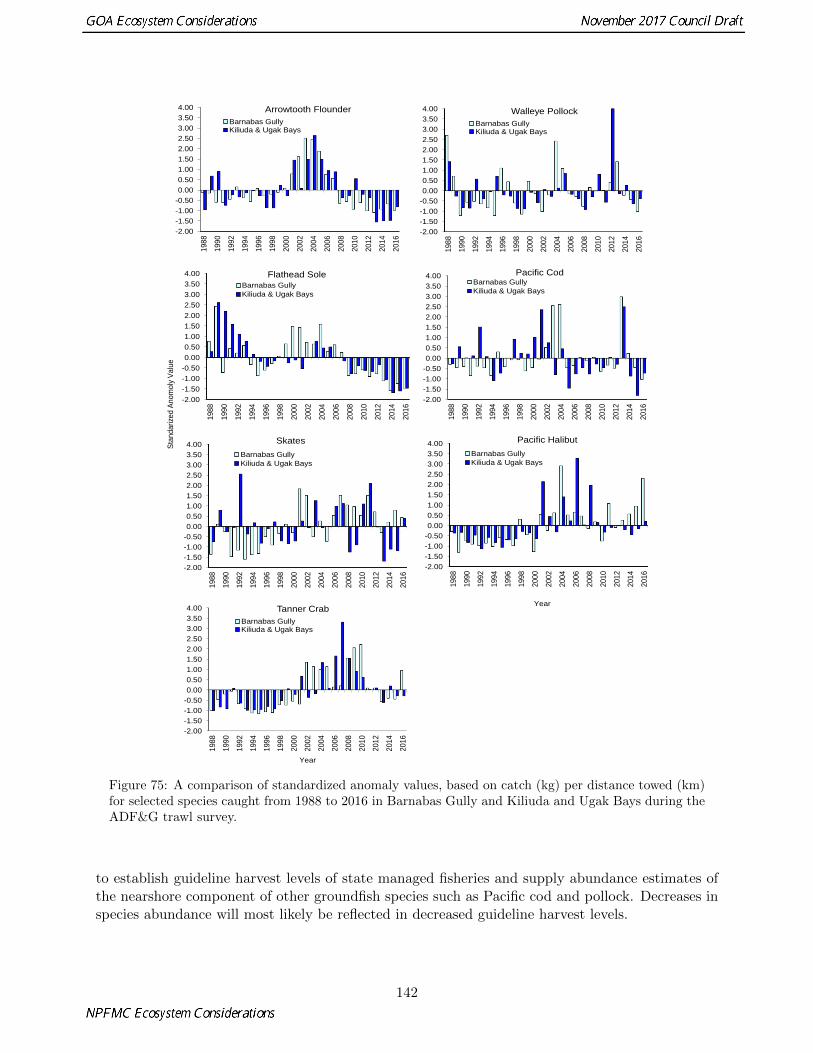
-2.00

-1.50

-1.00

-0.50

0.00

0.50

1.00

1.50

2.00

2.50

3.00

3.50

4.00

198

8

199

0

199

2

199

4

199

6

199

8

200

0

200

2

200

4

200

6

200

8

201

0

201

2

201

4

201

6

Flathead Sole

Barnabas Gully

Kiliuda & Ugak Bays

-2.00

-1.50

-1.00

-0.50

0.00

0.50

1.00

1.50

2.00

2.50

3.00

3.50

4.00

198

8

199

0

199

2

1994

199

6

199

8

200

0

200

2

200

4

200

6

200

8

201

0

201

2

201

4

201

6

Pacific CodBarnabas Gully

Kiliuda & Ugak Bays

-2.00

-1.50

-1.00

-0.50

0.00

0.50

1.00

1.50

2.00

2.50

3.00

3.50

4.00

198

8

199

0

199

2

199

4

199

6

199

8

200

0

200

2

200

4

200

6

200

8

201

0

201

2

201

4

201

6

Tanner Crab

Barnabas GullyKiliuda & Ugak Bays

-2.00

-1.50

-1.00

-0.50

0.00

0.50

1.00

1.50

2.00

2.50

3.00

3.50

4.00

198

8

199

0

199

2

199

4

199

6

199

8

2000

200

2

200

4

200

6

200

8

201

0

201

2

201

4

201

6

Arrowtooth Flounder


-2.00

-1.50

-1.00

-0.50

0.00

0.50

1.00

1.50

2.00

2.50

3.00

3.50

4.00

198

8

199

0

199

2

199

4

199

6

199

8

200

0

200

2

200

4

200

6

200

8

201

0

201

2

201

4

201

6

Skates

Barnabas Gully

Kiliuda & Ugak Bays

-2.00

-1.50

-1.00

-0.50

0.00

0.50

1.00

1.50

2.00

2.50

3.00

3.50

4.00

198

8

199

0

199

2

199

4

1996

199

8

200

0

200

2

200

4

2006

200

8

201

0

201

2

201

4

2016

Pacific Halibut

Barnabas Gully

Kiliuda & Ugak Bays

-2.00

-1.50

-1.00

-0.50

0.00

0.50

1.00

1.50

2.00

2.50

3.00

3.50

4.00

198

8

1990

199

2

199

4

1996

199

8

200

0

2002

200

4

200

6

200

8

201

0

201

2

201

4

201

6

Walleye Pollock


Sta

nd

arize

d A

no

mo

ly V

alu

e

Year

Year

Figure 75: A comparison of standardized anomaly values, based on catch (kg) per distance towed (km)for selected species caught from 1988 to 2016 in Barnabas Gully and Kiliuda and Ugak Bays during theADF&G trawl survey.

to establish guideline harvest levels of state managed fisheries and supply abundance estimates ofthe nearshore component of other groundfish species such as Pacific cod and pollock. Decreases inspecies abundance will most likely be reflected in decreased guideline harvest levels.

142

20162014201220102008200620042002200019981996199419921990

2.0

1.5

1.0

0.5

0.0

-0.5

-1.0

Year

Ano

ma

ly V

alu

e

Kiliuda amd Ugak Bays

Barnabas Gully

El Niño Weak

El Niño Moderate

El Niño Strong

El Niño Very Strong

Figure 76: Bottom temperature anomalies recorded from the ADF&G trawl survey for Barnabas Gullyand Kiliuda and Ugak Bays from 1990 to 2016, with corresponding El Nino years represented.

143

Recruitment Predictions for Sablefish in Southeast Alaska

Contributed by Ellen Yasumiishi, Kalei Shotwell, Dana Hanselman, Emily Fergusson, Auke BayLaboratories Division, Alaska Fisheries Science Center, National Marine Fisheries Service, NOAAContact: [email protected] updated: August 2017

Description of indicator: Biophysical indices from surveys in 2016 and salmon returns in 2017were used to predict the recruitment of sablefish to age-2 in 2017 and 2018 (Yasumiishi et al.,2015). Biophysical indices were collected during the southeast coastal monitoring (SECM) survey.The SECM survey has an annual survey of oceanography and fish in inside and outside waters ofnorthern southeast Alaska since 1997 (Orsi et al. 2012). Oceanographic sampling included, butwas not limited to, sea temperature and chlorophyll a. These data are available from documentspublished through the North Pacific Anadromous Fish Commission website from 1999 to 2012 (www.npafc.org) and from Emily Fergusson at the Alaska Fisheries Science Center in Juneau, Alaska.An index for pink salmon survival was based on adult returns of pink salmon to southeast Alaska(Piston and Heinl, 2014). These oceanographic metrics may index sablefish recruitment, becausesablefish use these waters as rearing habitat early in life (late age-0 to age-2). Estimates of age-2sablefish abundance are from (Hanselman et al., 2013). We modeled age-2 sablefish recruitmentestimates from 2001 to 2010 as a function of sea temperature, chlorophyll a, and pink salmonproductivity during the age-0 stage for sablefish.

Status and trends: We modeled age-2 sablefish recruitment estimates from 2001 to 2016 (Hansel-man et al., 2016) as a function of sea temperatures during 1999–2014, chlorophyll a during 1999–2014, and adult pink salmon returns in 2000–2015. The model with the lowest Bayesian informationcriterion (108) described the stock assessment estimates of age-2 sablefish abundance as a functionof late August maximum chlorophyll a during the age-0 stage, late August maximum sea temper-ature during the age-0 stage, and pink salmon returns during the age-1 life stage of these sablefish(Figure 77; Table 3). A regression model indicated positive coefficient for the predictor variableschlorophyll a, sea temperature, and pink salmon returns were positively in the sablefish model (R2

= 0.767, Adjusted R2 = 0.708, F-statistic: 13.15 on 3 and 12 DF, p-value: 0.0004).

Based on 2016 environmental data, the high levels of 10.83 chlorophyll a (10.83), warm waters(13.4oC) and good forecast for pink salmon returns (43 million) in 2017, we predict above averageabundance of age-2 sablefish (68 million) in 2018 (2016 year class). Based on 2017 environmentaldata, low chlorophyll a (1.12) in 2015, average sea temperatures (12oC), and low pink salmonreturns in 2016 (17,820,985), we predict below average abundance of age-2 sablefish in 2017 for the2015 year class.

144

www.npafc.org

www.npafc.org

Figure 77: Stock assessment estimates, model estimates, and the 2017 and 2018 prediction for age-2Alaska sablefish. Stock assessment estimates of age-2 sablefish were modeled as a function of late Augustchlorophyll a levels and late August sea temperatures in the waters of Icy Strait in northern southeastAlaska during the age-0 stage (t-2), and the returns of age-1 pink salmon (t-1). These predictors areindicators for the conditions experiences by age-0 sablefish. Stock assessment estimates of age-2 sablefishabundances are from Table 3.14 in Hanselman et al. (2016).

145

Table 3: Nearshore survey data fit to the stock assessment estimates of age-2 sablefish (millions of fish) from Hanselman et al. (2016). Tableshows the 2017 model fitted (2001–2016) and forecast (2017, 2018) estimates and standard errors for age-2 sablefish, and the predictor variablefrom 1999–2015 used to estimate (2001–2016) and predict (2017, 2018) the stock assessment estimates of age-2 sablefish. Values in bold indicatepredicted values based on the 2017 Model and environmental indices from 2016 and 2017.

Stock Assessment Model

Estimates Fitted and forecast Predictor variablesYear Sablefish (t) Estimates Standard error Chlorophyll a (t-2) Sea temperature (t-2) Pink salmon (t-1)2001 12.2 8.95 2.067 2.15 13.4 31,009,5472002 44.5 40 4.56 6.08 12 85,654,2262003 7.1 8.79 1.55 1.63 12.8 61,929,9242004 14 11.16 2.72 2.64 10.7 72,431,6232005 6.8 6.77 1.81 1.22 13.1 60,965,6612006 12 12.61 2.94 1.05 14.5 79,033,9172007 8.9 8.38 2.25 2.68 12.5 21,848,8502008 9.9 6.56 2.75 2.15 10.8 62,435,5992009 9.6 11.54 2.8 2.33 14.2 25,406,3772010 20.7 16.84 1.88 3.59 11.7 50,695,1142011 5.4 8.91 1.78 2.52 12.3 35,196,2812012 10.6 3.13 2.51 0.55 12.7 73,123,9472013 1.2 8.86 2.51 3.06 11.2 32,320,5952014 9.2 17.63 3.58 1.58 12.7 119,898,1912015 17.2 12.98 2.33 1.92 14.2 50,944,4322016 12.9 19.07 1.94 3.73 12.4 46,306,3932017 -4.11 3.3 1.12 12 17,820,9852018 68.72 10.08 10.83 13.4 43,000,000

Factors influencing observed trends: Warmer sea temperatures were associated with highrecruitment events in sablefish (Sigler and Zenger Jr., 1989). Higher chlorophyll a content insea water during late summer indicate higher primary productivity and a possible late summerphytoplankton bloom. Higher pink salmon productivity, a co-occurring species in near-shore waters,was a positive predictor for sablefish recruitment to age-2. These conditions are assumed morefavorable for age-0 sablefish, overwintering survival from age-0 to age-1, and overall survival toage-2.

Implications: Our 2017 model indicates that we should expect a weak 2015 year class and astrong 2016 year class of sablefish.

Distribution of Rockfish Species in Gulf of Alaska Trawl Surveys


Description of indicator: In a previous analysis of rockfish from 14 bottom trawl surveys in theGulf of Alaska and Aleutian Islands (Rooper, 2008), five species assemblages were defined basedon similarities in their distributions along geographical position, depth, and temperature gradients.The 180 m and 275 m depth contours were major divisions between assemblages inhabiting the shelf,shelf break, and lower continental slope. Another noticeable division was between species centeredin southeastern Alaska and those found in the northern Gulf of Alaska and Aleutian Islands.

In this time series, the mean-weighted distributions of six rockfish (Sebastes spp.) species alongthe three environmental gradients (depth, temperature, and position) were calculated for the Gulfof Alaska. A weighted mean value for each environmental variable was computed for each surveyas:

Mean =

∑(fixi)∑fi

,

where fi is the CPUE of each rockfish species group in tow i and xi is the value of the environmentalvariable at tow i. The weighted standard error (SE) was then computed as:

SE =

√(∑

(fix2i ))−((

∑fi)∗mean2)

(∑

fi)−1√n

,

where n is the number of tows with positive catches. Details of the calculations and analysescan be found in Rooper (2008). These indices monitor the distributions of major components ofthe rockfish fisheries along these environmental gradients to detect changes or trends in rockfishdistribution.

Status and trends: In the Gulf of Alaska, there continues to be no significant trends in thedistribution of rockfish with depth, temperature and position (Figure 78). This is in contrast tosome of the earlier years in which the indicator was calculated. The distribution of rockfish speciesin the bottom trawl surveys appears to have stabilized for the Gulf of Alaska.

147

Factors causing observed trends: In the Gulf of Alaska, the stability of the distribution indi-cates that each of the species occupy a fairly specific depth distribution. This is seen in the flatline time series of distribution across depths and the variability in temperature. As temperaturesrise and fall around the mean, the depth distribution does not change, indicating that the rockfishare not changing their habitat or distribution to maintain a constant temperature.

Implications: The trends in the mean-weighted distributions of rockfish should continue to bemonitored, with special attention to potential causes of the shift in depth and position distributionsof rockfish, especially as they relate to changing temperatures.

Figure 78: Plots of mean weighted (by catch per unit effort) distributions of six rockfish species-groupsalong three environmental variables in the Gulf of Alaska. Mean weighted distributions of rockfishspecies-groups are shown for A) position, B) depth, and C) temperature. Position is the distance fromHinchinbrook Island, Alaska, with positive values west of this central point in the trawl surveys andnegative values in southeastward. Asterisk indicates significant trend over the time series.

148

Benthic Communities and Non-target Fish Species

Miscellaneous Species – Gulf of Alaska Bottom Trawl Survey


Description of indicator: RACE bottom trawl surveys in the Gulf of Alaska (GOA) are designedprimarily to assess populations of commercially important fish and invertebrates. However manyother species are identified, weighed and counted during the course of these surveys, and these datamay provide a measure of relative abundance for some of these species. For each species group, thecatches for each year were scaled to the largest catch over the time series (which was arbitrarilyscaled to a value of 100). The standard error (+/- 1) was weighted proportionally to the CPUE toget a relative standard error. The percentage of positive catches in the survey bottom trawl haulswas also calculated.

Status and trends: Echinoderm catches have been highest in the Kodiak and Chirikof regions ofthe GOA, and they are consistently captured in ∼80% of bottom trawl hauls in all areas (Figure 79.Echinoderms have been declining in both of these areas over the last few surveys. Shrimp CPUEhas been increasing in the Kodiak and Chirikof areas over the last few surveys, while remainingfairly constant and low in the other areas. Eelpout CPUE has been variable, with peak abundancesoccurring in 1993, 2001 and 2009 in the Shumagin area, 2003 and 2013–2015 in the central GOA(Kodiak and Chirikof areas) and peak catches after 1999 in the eastern GOA. Poacher CPUEspeaked in 1993 and 2015 in the Shumagin area. Poachers have been uniformly in low abundancein the Chirikof, Yakutat and Southeastern areas and have been variable, but somewhat higher inthe Kodiak areas.

149

Figure 79: Relative mean CPUE of miscellaneous species by area from RACE bottom trawl surveys in the Gulf of Alaska from 1984 through2017. Error bars represent standard errors. The gray lines represent the percentage of non-zero catches.

Factors influencing observed trends: Many of these species are not sampled well by the gearor occur in areas that are not well sampled by the survey (hard, rough areas, mid-water etc.) andare therefore encountered in small numbers which may or may not reflect their true abundance inthe GOA. The fishing gear used aboard the Japanese vessels that participated in all GOA surveysprior to 1990 was very different from the gear used by all vessels since. This gear difference almostcertainly affected the catch rates for some of these species groups.

Implications: The trends in other species in the bottom trawl survey do not appear consistentover time, with the possible exception of decreases in recent echinoderm catches.

151

Seabirds

Seabird Monitoring Summary for the Western Gulf of Alaska

Contributed by Heather Renner, Nora Rojek, Arthur Kettle, Alaska Maritime National WildlifeRefuge, Homer, AKContact: heather [email protected] updated: October 2017

Description of indicator: The Alaska Maritime National Wildlife has monitored seabirds atcolonies around Alaska in most years since the early- to mid-1970’s. Time series of annual breedingsuccess and phenology (and other parameters) are available from over a dozen species at eightRefuge sites in the Gulf of Alaska, Aleutian Islands, and Bering and Chukchi Seas. Monitoredcolonies in the Gulf of Alaska include Aiktak (in Unimak Pass), Chowiet (Semidi Islands), EastAmatuli (Barren Islands), and St. Lazaria (Southeast Alaska; not monitored in 2017) islands.Reproductive success is defined as the proportion of nest sites with eggs (or just eggs for murresthat do not build nests) that fledged a chick.

Status and trends: Several fish-eating seabirds had unusually low reproductive success in 2017.At Chowiet Island in the Semidis, this included tufted and horned (not shown) puffins (Figure 80).Common murres, which showed rare widespread reproductive failure in 2015–2016, generally hadbetter colony attendance and fledging rates in 2017 but still the number of birds breeding was low.In 2017, tufted puffin productivity was >1 standard deviation (SD) below the long term mean atall monitored sites except at East Amatuli (where they were observed carrying large amounts ofcapelin). Black-legged kittiwakes and storm-petrels (which consume a mix of fish and invertebrates)showed fledging rates within 1 SD of the mean, as did planktivorous auklets. Timing of breedingwas within typical ranges for most species (although horned puffins and ancient murrelets wereearly at Aiktak and murres and kittiwakes were late at East Amatuli).

Factors influencing observed trends: In general, murres appear to have been negatively affectedduring the marine heat wave of the past few years, with widespread reproductive failures, die-offs,and low attendance at breeding colonies. Other species did not show broad-scale failures duringthis period; planktivorous seabirds were generally successful. Despite overall low reproductivesuccess of murres in 2017, some improvement in murre attendance and fledging success may reflectenvironmental changes returning back to more neutral conditions (see Bond, p. 56).

Implications: Reproductive activity of central-place foraging seabirds can reflect ecosystem con-ditions at multiple spatial and temporal scales. For piscivorous species that feed at higher trophiclevels, continued reduced reproductive success may indicate that the ecosystem has not yet shiftedback from warm conditions and/or there is a lagged response of the prey. However, the improve-ment in attendance and minimal reproductive activity among murres during 2017 indicates someimprovement in foraging conditions for those species.

152

-10

40

90 Common Murres at the Semidis

-10

40

90 Tufted Puffins at the Semedis

-10

30

70

Black-legged Kittiwakes at the Semidis

-10

35

80 Parakeet Auklets at the Semidis

1989 1995 2000 2005 2010 2017

2013-2017 Mean 2013-2017 Trend

1 s.d. above mean

1 s.d. below mean







Figure 80: Summary of reproductive success for select seabird species at Chowiet Island in the Semidis.

153

Marine Mammals

Humpback Whale Calving and Juvenile Return Rates in Glacier Bay and Icy Strait

Contributed by Janet Neilson, Christine Gabriele, Louise Taylor-Thomas, Glacier Bay NationalPark and Preserve, P.O. Box 140, Gustavus, AK 99826Contact: janet [email protected] updated: September 2017

Description of indicator: From 1985–2017, we used consistent methods and levels of effort tomonitor humpback whales annually from June 1–August 31 in Glacier Bay and Icy Strait (Gabrieleet al., 2017). We calculated the crude birth rate as an annual index of reproduction by dividingthe number of calves by the total whale count each year. We also documented the return andrecruitment of calves into the population as juveniles. Humpback whales and groundfish target thesame lipid-rich prey (i.e., forage fish and euphausiids) and trends in humpback whale reproductivesuccess and juvenile survival may indicate changes in prey availability and/or quality in the easternGulf of Alaska.

Status and trends: There is mounting evidence that humpback whale calving and juvenile returnrates in Glacier Bay and Icy Strait have declined substantially in recent years. In 1985–2013, weobserved 2–21 calves per year (mean = 9.3) and a crude birth rate ranging 3.3%–18.2% (Figure 81).Females almost always remained with their calves for the entire summer although we documenteda missing calf in eight cases over the 1985–2013 time period, with no more than one case per year(Neilson et al., 2015). In 2014, an unprecedented number of calves (n = 5) went missing betweenearly August and late October (Neilson et al., 2015) and none of the remaining calves (n = 9) havebeen resighted in subsequent years. In 2015, we documented relatively few calves (n = 5) (Neilsonand Gabriele, 2016) and none have been resighted. In 2016, we documented only one mother/calfpair (both appeared to be abnormally thin), which led to the lowest crude birth rate (0.6%) sincemonitoring began in 1985 (Neilson et al. 2017) (Figure 81). In 2017, we documented only twomother-calf pairs, which we expect will lead to an anomalously low crude birth rate for the secondyear in a row (the total whale count for 2017 is pending data analysis). Furthermore, one of themothers in 2017 appeared to be abnormally thin and the other lost her calf by mid-July.

Humpback whales that summer in southeastern Alaska exhibit strong maternally-directed sitefidelity that has driven population growth over time (Pierszalowski et al., 2016). We did notdocument any one or two-year-old whales in 2016 and we observed very few small whales in 2017.Out of 29 calves that we documented in the study area from 2013–2015, only two individuals (7%)are known to have survived to be juveniles in the study. While the mean age at which calves returnto the study area is 3.2 years (Gabriele et al., 2017) and juvenile whales can be difficult to track andphoto-identify based on their small size and often erratic behavior, it is notable that before 2016,the last time we documented no one- or two-year-old whales in the study area was 2003 (Figure82).

Factors influencing observed trends: We hypothesize that these changes in calving and juvenilereturn rates may be related to recent changes in whale prey availability and/or quality, which mayin turn be negatively affecting maternal body condition and therefore reproductive success and/oroverall juvenile survival (Bradford et al., 2012; Fuentes et al., 2016; Seyboth et al., 2016). This

154

Figure 81: Crude birth rate (black line) (1985–2016) and annual number of calves (blue bars) (1985–2017) in Glacier Bay-Icy Strait.

Figure 82: Number of calves, one- and two-year-old whales documented annually in Glacier Bay-IcyStrait, 2003–2016.

hypothesis is supported by observed declines in the body condition of humpback whales throughoutnorthern Southeast Alaska in recent years (see Moran et al. this report).

Implications: Recruitment from local populations (vs. immigration from outside populations) hasbeen a key driver of humpback whale population growth over the past 30 years in Glacier Bay andIcy Strait (Pierszalowski et al., 2016), therefore sustained declines in calving and/or recruitmentwill have long-term effects on the humpback whale population in this area. If humpback whales

155

are currently food-limited in northern Southeast Alaska, this might indicate that groundfish (whichprey on the same species) may also be food-limited.

Summer Survey of Population Level Indices for Southeast Alaska Humpback Whales

Contributed by John Moran11, Christine Gabriele, Janet Nielson, Heidi Pearson, Andy Szabo,Steve Lewis, Janice Straley, Jennifer Cedarleaf11Auke Bay Laboratories Division, Alaska Fisheries Science Center, National Marine Fisheries Ser-vice, NOAAContact: [email protected] updated: October 2017

Description of indicator: Humpback whale populations have been monitored by various orga-nizations in Northern Southeast Alaska since the 1970. The Survey of Population Level Indicesfor Southeast Alaska Humpback (SPLISH) survey assessed trends in abundance, calf production,spatial and temporal distribution, prey composition, and body condition for humpback whales inNorthern Southeast Alaska during 2016 and 2017 (data from 2017 are not yet available). The 2016results can be compared to earlier studies to produce a decadal-scale time series (Straley et al.,2009; Calambokidis et al., 2008; Hendrix et al., 2012; Dahlheim et al., 2009; Neilson et al., 2017).For this report, we include the total number of juvenile/adult whales and calves estimated forFrederick Sound, Stephens Passage, Glacier Bay, and Icy Strait.

Status and trends: The total number of whales has increased each decade. Crude birth rateswere highest in 1986 and lowest in 2016. Calf numbers in 2017 are expected to be similar to 2016or lower. There has been a recent decrease in observed body condition (not shown). There is alsoanecdotal evidence that whales have shifted the distribution to the continental shelf from insidewater such as SEAK and Prince William Sound, possibly to feed on euphausiids.

During September in Prince William Sound, lower numbers of humpback whales and marine birdswere observed along with a record low biomass of herring, and low numbers of other forage fishand krill relative to previous years. This was our 7th fall survey, with the lowest number of whalessince the project began in 2007 (Table 4). Increased effort and excellent conditions while surveyingknown whale/herring hot spots failed to locate any concentrations of humpbacks or prey.

Factors influencing observed trends: Potential causes for observed trends and current statusinclude: recent abnormally warm water in the Gulf of Alaska, which has been linked to decreasingprimary production/ forage species; humpback whale populations approaching carrying capacity;or a shift in whale distribution (i.e. offshore to better feeding grounds).

Regarding the Prince William Sound survey, the decline in whales mirrors the decline in herringwithin the Sound. The PWS herring biomass had been hovering around 20,000 tonnes in since1993. In 2015 it dropped to 8000 tonnes and continued to decline in 2016 and 2017 to 3000–3500tonnes (pers. comm. Scott Pegau). Mile days of spawn have dropped from a range of 150 milesprior to the spill, to about 50 miles in the “re-set” level of the 90s and 2000s, to a downward spiralof 36 mile days in the El Nino year of 2014, to 17 mile days in the “Blob” year of 2015, and to 9mile days in 2016, and 9 mile days in 2017. These levels are unprecedented, and not capable ofsupporting the predator levels of previous years.

156

9 mile days in 2016, and 9 mile days in 2017. These levels are unprecedented, and not capable of supporting the predator levels of previous years.

Implications: These observations suggest that there is a long-term trend in humpback whales in Gulf of Alaska that may be related to prey. If prey is limiting and humpback whale populations have fully recovered to carrying capacity, there is potential for top-down forcing on forage species (Moran et. al. 2017: Straley et. al. 2017) and competition with fish, other marine mammals, and seabirds. Monitoring humpback whale indicators may be useful in assessing productivity in the eastern GOA (i.e. shifts in whale distribution may reflect shifts in prey; changes in body condition and calf production may indicate changes in prey abundance or availability). Since there is significant prey overlap between humpback whales and many ground fish species, these data may be useful for a coarse evaluation of ground fish forage.

Figure 1. Total numbers of humpback whales, calves and crude birth rate in Frederick Sound, Stephens Passage, Glacier Bay, and Icy Strait.

Literature Cited

Moran, J. R., R. A. Heintz, J. M. Straley, and J. J. Vollenweider. 2017. Regional variation in the intensity of humpback whale predation on Pacific herring in the Gulf of Alaska. Deep Sea Research Part II: Topical Studies in Oceanography.

Straley, J. M., J. R. Moran, K. M. Boswell, R. A. Heintz, T. J. Quinn II, B. Witteveen, and S. D. Rice. 2017. Seasonal presence and potential influence of foraging humpback whales upon Pacific herring wintering in the Gulf of Alaska. Deep Sea Research Part II: Topical Studies in Oceanography.

0%

5%

10%

15%

20%

0

50

100

150

200

250

1986 1998 2004 2016

# of

Wha

les

All whales Calves % CalvesFigure 83: Total numbers of humpback whales, calves and crude birth rate in Frederick Sound, StephensPassage, Glacier Bay, and Icy Strait.

Table 4: Index of PWS humpback whale abundance in PWS. * Note that the 2007 survey did notcover Montague Entrance, an area known for the highest concentration of whales and herring withinthe Sound in September.

Month/yearCountsof whales

Nautical milessurveyed

Encounter rateWhale/NM

Sep 2007* 24 370 0.06Sep 2008 71 412 0.17Oct 2011 62 441 0.14Sep 2012 81 444 0.18Sep 2013 113 355 0.32Sep 2014 181 427 0.42Sep 2017 12 543 0.02

Implications: These observations suggest that there is a long-term trend in humpback whales inGulf of Alaska that may be related to prey. If prey is limiting and humpback whale populations havefully recovered to carrying capacity, there is potential for top-down forcing on forage species (Moranet al., 2017; Straley et al., 2017) and competition with fish, other marine mammals, and seabirds.Monitoring humpback whale indicators may be useful in assessing productivity in the eastern GOA(i.e. shifts in whale distribution may reflect shifts in prey; changes in body condition and calfproduction may indicate changes in prey abundance or availability). Since there is significant preyoverlap between humpback whales and many ground fish species, these data may be useful for acoarse evaluation of ground fish forage.

157

Ecosystem or Community Indicators

Aggregated Catch-Per-Unit-Effort of Fish and Invertebrates in Bottom Trawl Surveysin the Gulf of Alaska, 1993–2017

Contributed by Franz Mueter, University of Alaska Fairbanks, 17101 Point Lena Road, Juneau,AK 99801Contact: [email protected] updated: October 2017

Description of indicator: This index provides a measure of the overall biomass of benthic, dem-ersal, and semi-demersal fish and invertebrate species. We obtained catch-per-unit-effort (CPUE inkg ha-1) of fish and major invertebrate taxa for each successful haul completed during standardizedbottom trawl surveys on the Gulf of Alaska shelf (GOA), 1993–2017. Total CPUE for each haulwas computed as the sum of the CPUEs of all fish and invertebrate taxa. To obtain an index ofaverage CPUE by year, we modeled log-transformed total CPUE (N = 6333 and 1561 hauls in thewestern (west of 147oW) and eastern GOA, respectively) as smooth functions of depth, alongshoredistance and sampling stratum with year-specific intercepts using Generalized Additive Models fol-lowing Mueter et al. (2002). Hauls were weighted based on the area represented by each stratum.To avoid biases due to gear and vessel issues, data prior to the 1993 survey was not included in theanalysis.

Status and trends: Total log(CPUE) in both the eastern and western GOA decreased from recenthigh values to their lowest (west) and second lowest (east) value in 2017 (Figure 84). There wasno significant long-term trend over time from 1993 to 2017 in either region, but total CPUE de-creased significantly by 30–40% since 2009 and 2013, respectively, in the eastern and western GOA.The decrease in CPUE was widespread among species, affecting commercial and non-commercialspecies. Species that showed the largest absolute declines in biomass since 2013 included walleyepollock, Pacific cod, arrowtooth flounder and northern rockfish in the western GOA; and arrowtoothflounder, shortraker rockfish, Pacific cod and spiny dogfish in the eastern GOA.

Factors influencing observed trends: Commercially harvested species account for over 70% oftotal survey catches. Fishing is expected to be a major factor determining trends in survey CPUE,but environmental variability is likely to account for a substantial proportion of the observed vari-ability in CPUE through variations in recruitment, growth, and distribution. Substantial declinesin many species in recent years may be associated with the unusual warm conditions in the GOA in2014–2016, which appeared to affect prey availability and were associated with unusual mortalityevents in seabirds and marine mammals.

Implications: This indicator can help address concerns about maintaining adequate prey forupper trophic level species and other ecosystem components. A sharp drop in total biomass ofdemersal fish and invertebrates affecting commercial and non-commercial species, suggests pooravailability of zooplankton prey for these species and a reduced prey base for upper trophic levelspecies following the 2014/15 warm event.

158

Figure 84: Model-based estimates of total log(CPUE) for major fish and invertebrate taxa capturedin bottom trawl surveys from in the western (west of 147oW) and eastern Gulf of Alaska by surveyyear with approximate 95% confidence intervals. Estimates were adjusted for differences in depth andsampling locations (alongshore distance) among years. No sampling in the eastern Gulf of Alaska in2001.

159

Average Local Species Richness and Diversity of the Gulf of Alaska Groundfish Com-munity

Contributed by Franz Mueter, University of Alaska Fairbanks, 17101 Point Lena Road, Juneau,AK 99801Contact: [email protected] updated: October 2017

Description of indicator: Indices of local species richness and diversity are based on standardbottom trawl surveys in the western (WGOA; west of 147oW) and eastern Gulf of Alaska (EGOA).We computed the average number of fish and major invertebrate taxa per haul (richness) and theaverage Shannon index of diversity (Magurran, 1988) by haul based on CPUE (by weight) of eachtaxon. Indices for the Gulf of Alaska were based on 76 fish and common invertebrate taxa thathave been consistently identified since the early 1990s. Indices were computed following (Mueteret al., 2002). Briefly, annual average indices of local richness and diversity were estimated byfirst computing each index on a per-haul basis, then estimating annual averages with confidenceintervals across the survey area using a Generalized Additive Model that accounted for the effectsof variability in geographic location (latitude/longitude) and depth with year-specific intercepts.In addition to trends in the indices over time, we mapped average spatial patterns for each indexacross the survey region.

Status and trends: Richness and diversity were generally higher in the EGOA than in the WGOAwith, on average, 2–3 additional species per haul in the east (Figure 85). Richness and diversityhave been relatively stable in the western Gulf with slightly higher local richness in the 2015/17surveys compared to the 2011/13 surveys. Local species richness in the eastern Gulf increasedsubstantially in 2013, declined by more than 2 species per haul in 2015 and increased somewhat in2017. Diversity in the EGOA had been declining since 2007 but increased in the most recent surveyassociated with the increase in local richness (Figure 85). Both richness and diversity tend to behighest along the shelf break and slope (Figure 86), with richness peaking at or just below the shelfbreak (200–300m), and diversity peaking deeper on the slope (300m+), as well as in some shallowwater regions (< 100m). Notably, both richness and diversity are high off the Kenai Peninsula.

Factors influencing observed trends: Local richness and diversity reflect changes in the spatialdistribution, abundance and species composition that may be caused by fishing, environmentalvariability, or climate change. If species are, on average, more widely distributed in the samplingarea the number of species per haul increases. Local species diversity is a function both of how manyspecies are caught in a haul and how evenly CPUE is distributed among these species, hence timetrends (Figure 85) and spatial patterns (Figure 86) in species diversity differ from those in speciesrichness. Diversity typically increases with species richness and decreases when the abundance ofdominant species increases. For example, the decreasing trend in diversity in the EGOA since2007 appears to be due to an increase in the abundance and dominance of a few species, includingarrowtooth flounder, walleye pollock and Pacific ocean perch. The unusual increase in local speciesrichness in the EGOA in 2013 appears to have resulted from increased catches of a number of fishand invertebrate species, including walleye pollock, several Sebastes species, skates, grenadiers, seastars and others. The increase in richness and diversity in 2017 reflects reduced dominance of manyof these species and possibly a more even distribution across space.

Implications: There is evidence from many systems that diversity is associated with ecosystem

160

Figure 85: Model-based annual averages of species richness (average number of species per haul, toppanels) and species diversity (Shannon index, bottom panels), 1993–2017, for the Western (left) andEastern (right) Gulf of Alaska based on, respectively, 74 and 73 fish and invertebrate taxa collected bystandard bottom trawl surveys with 95% pointwise confidence intervals. Model means were adjustedfor differences in depth, date of sampling, and geographic location.

stability, which depends on differential responses to environmental variability by different speciesor functional groups (McCann, 2000). To my knowledge, such a link has not been established formarine fish communities.

161

Figure 86: Average spatial patterns in local species richness (species per haul, top panels) and Shannondiversity (bottom panels) for the Western (left) and Eastern (right) Gulf of Alaska.

162

Disease Ecology Indicators

“Mushy” Halibut Syndrome Occurrence

Contributed by Stephani ZadorResource Ecology and Fisheries Management Division, Alaska Fisheries Science Center, NationalMarine Fisheries Service, NOAAContact: [email protected] updated: October 2016

Description of indicator: The condition was first detected in Gulf of Alaska halibut in 1998.Increased prevalence occurred in 2005, 2011, and 2012, while it was apparently absent in 2013and 2014. It is most often observed in smaller halibut of 15–20 lbs in the Cook Inlet area, buthas also been noted in Kodiak, Seward, and Yakutat. Alaska Department of Fish and Game(ADF&G) describes the typical condition consisting of fish having large areas of body muscle thatare abnormally opaque and flaccid or jelly-like. The overall body condition of these fish is usuallypoor, and often they are released because of the potential inferior meat quality. Incidence of mushyhalibut is reported opportunistically in recreational fishing reports, but may not represent truetrends.

Status and trends: ADF&G post samplers have reported relatively few “mushy” halibut duringthe 2017 sport fishing season (http://www.adfg.alaska.gov/sf/fishingreports/).

Factors influencing observed trends: The condition is considered a result of nutritional my-opathy/deficiency, and thus may be indicative of poor prey conditions for halibut. According toADF&G, the Cook Inlet and Homer/Seward areas are nursery grounds for large numbers of younghalibut that feed primarily on forage fish that have recently declined in numbers. Stomach contentsof smaller halibut now contain mostly small crab species. Whether this forage is deficient, eitherin quantity or in essential nutrients is not known. However, mushy halibut syndrome is similarto that described for other animals with nutritional deficiencies in vitamin E and selenium. Thismuscle atrophy would further limit the ability of halibut to capture prey possibly leading to furthermalnutrition and increased severity of the primary nutritional deficiency.

Implications: The relatively few reports of “mushy” halibut, particularly relative to its recentprevalence in 2015 and 2016, may indicate that foraging conditions for young halibut were morefavorable during the past year. However, reporting is opportunistic and may not reflect trueprevalence.

Ichthyophonus Parasite

Contributed by the Fisheries, Aquatic Science, and Technology (FAST) Lab, Alaska Pacific Uni-versity.Contact: [email protected] updated: August 2017

Description of indicator: Ichthyophonus (spp.) is a globally distributed mesomycetozoan fish

163

http://www.adfg.alaska.gov/sf/fishingreports/

parasite, which has caused epizootic events among economically important fish stocks, includingherring and salmon. The parasite has been documented in at least 145 fish species, and infectioncan result in reduced growth, stamina, and overall health. In some cases, individuals show grossclinical signs including black papules, white nodules on heart tissue, muscle ulcers, and rougheningof the skin. The FAST Lab has conducted Ichthyophonus surveys since 2011 that have focused oncommon sport-caught fishes throughout the marine waters of southcentral Alaska.

Current work is focused on surveying Ichthyophonus prevalence in Pacific halibut for 2017 in Homer.This work uses a fish length-based sampling design and also examines physiological componentsto gain more information on how the parasite affects halibut condition. Bioelectric impedanceanalysis (BIA) and Fultons Condition Factor (K) are being used to assess muscle condition andlength/weight ratio. In addition, host immune response to the parasite is being measured byhistolopathological methods, and qPCR is being used to quantify parasite load. As with our earlierresearch, we are working cooperatively with the ADF&G port sampling program and the charterhalibut fleets.

Status and trends: Initial work in August of 2011 resulted in the first documentation of nat-ural Ichthyophonus infections in lingcod (Ophiodon elongates), yelloweye rockfish (Sebastes ruber-rimus) and Pacific cod (Gadus macrocephalus), along with the expansion of the geographic rangeof Ichthyophonus in black rockfish (Sebastes melanops) northward to include southcentral Alaska(Harris et al., InReview).

Subsequent work has focused on Pacific halibut (Hippoglossus stenolepis) in Homer, Alaska. Themost recent survey was performed in 2016, and found 57% prevalence (n=335). Previous surveysreported 26% (n=126, 2011), 29% (n=248, 2012) and 23% (n=315, 2013)(Grenier, 2014).

Factors influencing observed trends: The 2012 and 2013 FAST Lab Pacific halibut researchfound that the parasite infected heart tissues; was never found in liver, spleen, or kidney tissues;and was more prevalent in older fish. A pepsin digestion assay was developed to assess the degreeof infection, and found that load varied widely among infected fish with 6 to 1,245 Ichthyophonusschizonts per gram of heart tissue. Findings did not support the hypothesis that reduced halibutsize-at-age may be caused by Ichthyophonus.

Implications: This research has found no indication of high intensity infections or clinically dis-eased individuals. These results support the hypothesis that under typical conditions, Ichthyophonuscan occur at high infection prevalence with concomitant low infection intensities. This project laysimportant methodological groundwork for the expansion of groundfish condition research to theBering Sea, Aleutian Islands and Gulf of Alaska.

164

Fishing and Human Dimensions Indicators

Indicators presented in this section are intended to provide a summary of the status of severalecosystem-scale indicators related to fishing and human economic and social well-being. Theseindicators are organized around objective categories derived from U.S. legislation and current man-agement practices (see Table 1 for a full list of objective categories and resulting indicators):

� Maintaining diversity

� Maintaining and restoring fish habitats

� Sustainability (for consumptive and non-consumptive uses)

� Seafood production

� Profits

� Recreation

� Employment

� Socio-cultural

The indicators presented are meant to represent trends in different aspects of the general manage-ment objective, but some indicators are better proxies than others. For example, seafood productionis a fairly good proxy for the production of seafood to regional, national, and international mar-kets but ex-vessel and wholesale value are imperfect proxies for harvesting and processing sectorprofits. This suite of indicators will continue to be revised and updated to provide a more holisticrepresentation of human/environment interactions and dependencies.

Maintaining Diversity: Discards and Non-Target Catch

Time Trends in Groundfish Discards

Contributed by Jean Lee, Resource Ecology and Fisheries Management Division, AFSC, NMFS,NOAA, and Alaska Fisheries Information Network, Pacific States Marine Fisheries CommissionContact: [email protected] updated: September 2017

Description of indicator: Estimates of groundfish discards for 1993–2002 are sourced from NMFSAlaska Regions blend data, while estimates for 2003 and later come from the Alaska Region’s CatchAccounting System. These sources, which are based on observer data in combination with industrylanding and production reports, provide the best available estimates of groundfish discards. Discardrates as shown in Figure 87 below are calculated as the weight of groundfish discards divided bythe total (i.e., retained and discarded) catch weight for the relevant area-gear-target sector. Whererates are described below for species or species groups, they represent the total discarded weightof the species/species group divided by the total catch weight of the species/species group for

165

the relevant area-gear-target sector. These estimates include only catch of Fishery ManagementPlan (FMP)-managed groundfish species on FMP-managed groundfish targets: not included aregroundfish discards in the halibut fishery and discards of non-FMP groundfish species, such asforage fish and species managed under prohibited species catch limits.

Figure 87: Total biomass and percent of total catch biomass of managed groundfish discarded in thefixed gear, pollock trawl, and non-pollock trawl sectors, 1993–2016 (Includes only catch counted againstfederal Total Allowable Catches).

Status and trends: Since 1993 discard rates of groundfish species in federally-managed Alaskangroundfish fisheries have generally declined in both pollock and non-pollock trawl fisheries in theGulf of Alaska (GOA)(Figure 87). One exception is in the GOA fixed gear sector, where rates havevaried between a low of 6% in 2012 and a high of 14% in 1993 and have trended upward since 2012following a downward decline during the preceding 4 year period. In the non-pollock trawl sector,discard rates dropped from 40% in 1994 to 21% in 1998, trended upwards from 1998 to 2003, andhave generally declined over the last ten years to a low of 8% in 2015 and 2016. Discard rates inthe GOA pollock trawl sectors declined from over 10% in 1993 to about 1% in 1998 and have sincefluctuated between 1% and 3%.

Factors influencing observed trends: Since the early 1990s fisheries managers in North Pacificgroundfish fisheries have employed various measures to address the problem of discards, including:

� Limited access privilege programs (LAPPs) that reduce economic discards by removing the

166

race for fish

� In-season closure of fisheries once target or bycatch species quotas are reached

� Minimum retention and utilization standards for certain fisheries

� Maximum retainable amounts (MRAs) specifying the amounts of “bycatch only” speciesthat harvesters may retain relative to other groundfish species that remain open to directedfishing. MRAs reduce regulatory discards by allowing for limited retention of species harvestedincidentally in directed fisheries.

In the Gulf of Alaska ecosystem management and conservation measures aimed at reducing by-catch have contributed to an overall decline in groundfish discards over time. Pollock roe stripping,wherein harvesters extract only the highest value pollock product and discard all of the remainingfish, was prohibited in 1991. In 1997 arrowtooth flounder was added as a basis species for retentionof pollock and Pacific cod, and in 1998 full retention requirements for pollock and cod were imple-mented for all vessels fishing for groundfish, leading to overall declines in pollock and cod discardsin the GOA. Additional retention requirements went into effect in 2003 for shallow-water flatfishspecies across the entire GOA and in 2004 for demersal shelf rockfish in the Southeast Outsidedistrict of the Eastern Gulf. Under the GOA groundfish FMP, fisheries with discard rates over 5%for shallow-water flatfish are subject to annual review by the North Pacific Council. Reductionsin flatfish discards account for most of the general decline in discards and discard rates for thenon-pollock trawl sector.

Implementation of the Pacific Halibut and Sablefish Individual Fishing Quota (IFQ) Program in1995 led to an overall decline in groundfish discards in the GOA longline sablefish fishery. The IFQprogram includes a number of measures to minimize discards of both target and bycatch species.Retention of sablefish and halibut is required as long as the harvester has IFQ catch quota available,which restricts the practice of high grading (discard of lower quality fish). Additionally, all Pacificcod and rockfish must be retained when IFQ halibut or sablefish are on board, subject to otherregulations.

Another LAPP, the Central Gulf of Alaska Rockfish Program, rationalizes allocations of rockfishspecies targeted with trawl gear in the Central GOA (northern rockfish, Pacific ocean perch, anddusky rockfish) along with species harvested incidentally in the fishery (Pacific cod, rougheyerockfish, shortraker rockfish, and sablefish). Vessels fishing in cooperatives with Rockfish Programquota are prohibited from discarding catch of rationalized species. Discards and discard rates ofsablefish and rockfish across the entire GOA non-pollock trawl sector have generally declined sincethe Rockfish Program was piloted in 2007.

In recent years the species historically comprising the “other groundfish” assemblage (skate, sculpin,shark, squid, octopus) have overtaken flatfish as the largest source of discards in the GOA. Mostdiscards of these species currently occur in the longline fishery, although greater observer coverageon smaller hook and line vessels beginning in 2013 likely accounts for some of the recent increasein fixed gear sector discards. Retention rates for skate and octopus have fluctuated over time,in part due to changing market conditions for these species. Interest in retention of skates anddirected fishing for skates (despite their management under “bycatch-only” status beginning in2005) resulted in annual overages of longnose and big skate TACs from 2007 to 2013. Discardsof skate have increased since 2012 as NMFS has taken action to prevent such overages, including

167

regulatory discard requirements for big skate in the Central GOA, imposed at progressively earlierdates from 2013 to 2015, and, in 2016, a reduction in the MRA for GOA skates from 20% to 5%.

Implications: Characterizing fishery bycatch, which includes discards of groundfish, is an im-portant component of ecosystem-based management. Discards add to the total human impact onbiomass without providing a benefit to the Nation and as such are seen as “contrary to responsiblestewardship and sustainable utilization of marine resources” (Kelleher, 2005). Bycatch in generalconstrains the utilization of commercial species (resulting in forgone income) and increases theuncertainty around total fishing-related mortality, making it more difficult to assess stocks, defineoverfishing levels, and monitor fisheries for overfishing. Although ecosystem effects of discards arenot fully understood, discards of whole fish and offal have the potential to alter energy flow withinecosystems and have been observed to result in changes to habitat (e.g., oxygen depletion in thebenthic environment) and community structure (e.g., increases in scavenger populations).

Minimizing fishery discards is recognized as an ecological, economic, and moral imperative in var-ious multilateral initiatives and in National Standard 9 of the Magnuson-Stevens Fishery Conser-vation and Management Act. Over the last three decades, management measures in North Pacificgroundfish fisheries have generally been effective in increasing groundfish retention and utiliza-tion and reducing discards. Monitoring discards and discard rates provides a way to assess thecontinuing efficacy of such measures.

168

Time Trends in Non-Target Species Catch

Contributed by Andy Whitehouse1, Sarah Gaichas2, and Stephani Zador31Joint Institute for the Study of the Atmosphere and Ocean (JISAO), University of Washington,Seattle WA,2Ecosystem Assessment Program, Northeast Fisheries Science Center, National Marine FisheriesService, NOAA, Woods Hole MA,3Resource Ecology and Fisheries Management Division, Alaska Fisheries Science Center, NationalMarine Fisheries Service, NOAAContact: [email protected] updated: September 2017

Description of indicator: We monitor the catch of non-target species in groundfish fisheries in theGulf of Alaska (GOA). In previous years we included the catch of “other” species, “non-specified”species, and forage fish in this contribution. However, stock assessments have now been developedor are under development for all groups in the “other species” category (sculpins, unidentifiedsharks, salmon sharks, dogfish, sleeper sharks, skates, octopus, squid), some of the species in the“non-specified” group (giant grenadier, other grenadiers), and forage fish (e.g., capelin, eulachon,Pacific sand lance, etc.), therefore we no longer include trends for these species/groups here (seeAFSC stock assessment website at http://www.afsc.noaa.gov/refm/stocks/assessments.htm).Invertebrate species associated with Habitat Areas of Particular Concern, previously known asHAPC biota (seapens/whips, sponges, anemones, corals, and tunicates) are now referred to asstructural epifauna. Starting with the 2013 Ecosystem Considerations Report, the three categoriesof non-target species we continue to track here are:

1. Scyphozoan jellyfish

2. Structural epifauna (seapens/whips, sponges, anemones, corals, tunicates)

3. Assorted invertebrates (bivalves, brittle stars, hermit crabs, miscellaneous crabs, sea stars,marine worms, snails, sea urchins, sand dollars, sea cucumbers, and other miscellaneousinvertebrates).

Total catch of non-target species is estimated from observer species composition samples taken atsea during fishing operations, scaled up to reflect the total catch by both observed and unobservedhauls and vessels operating in all Fishery Management Plan areas. Catch since 2003 has beenestimated using the Alaska Region’s Catch Accounting System. This sampling and estimationprocess does result in uncertainty in catches, which is greater when observer coverage is lower andfor species encountered rarely in the catch.

The catch of non-target species/groups from the GOA includes the reporting areas 610, 620, 630,640, 649, 650, and 659 (https://alaskafisheries.noaa.gov/sites/default/files/fig3.pdf). Within re-porting area 610, the GOA and Aleutian Islands (AI) Large Marine Ecosystems are divided at164oW. Non-target species caught east of 164oW is within the GOA LME and the catch west of164oW is within the AI LME.

Status and trends: The catch of Scyphozoan jellies in the GOA has been variable from 2011–2016, with the highest catch in 2016 (Figure 88). Other years of elevated catch were 2012 and 2015

169


and were preceded by years of reduced catch. Scyphozoan jellies are primarily caught in the pollockfishery. The catch of structural epifauna in the GOA dropped slightly from 2011 to 2012 and hasgenerally trended upward since. Sea anemones comprise the majority of the structural epifaunacatch and they are primarily caught in the flatfish, Pacific cod, and sablefish fisheries. The catchof assorted invertebrates in the GOA has been variable and shown little trend. Sea stars dominatethe assorted invertebrate catch, accounting for more than 90% of the total assorted invertebratecatch in each year. Sea stars are caught primarily in the Pacific cod and halibut fisheries. Thecatch of assorted invertebrates in 2015 increased 69% from 2014, and was the highest over the timeperiod 2011–2016. In 2016 the catch of assorted invertebrates dropped back down to nearly the2014 level.

Factors influencing observed trends: The catch of non-target species may change if fisherieschange, or ecosystems change, or both. Because non-target species catch is unregulated and unin-tended, if there have been no large-scale changes in fishery management in a particular ecosystem,then large-scale signals in the non-target catch may indicate ecosystem changes. Catch trends maybe driven by changes in biomass or changes in distribution (overlap with the fishery) or both. Fluc-tuations in the abundance of jellyfish are influenced by a suite of biophysical factors affecting thesurvival, reproduction, and growth of jellies including temperature, wind-mixing, ocean currents,and prey abundance (Purcell, 2005; Brodeur et al., 2008).

Implications: The catch of structural epifauna and assorted invertebrates is very low comparedwith the catch of target species. The lack of a clear trend in the catch of scyphozoan jellyfish mayreflect interannual variation in jellyfish biomass or changes in the overlap with fisheries. Abundantjellyfish may have a negative impact on fishes as they compete with planktivorous fishes for preyresources (Purcell and Sturdevant, 2001), and additionally, jellyfish may prey upon the early lifehistory stages (eggs and larvae) of fishes (Purcell and Arai, 2001; Robinson et al., 2014).

Stock Compositions of Chinook Salmon Bycatch in Gulf of Alaska Trawl Fisheries

Contributed by Jordan T. Watson, Chuck M Guthrie, Andrew Gray, Auke Bay Laboratories Divi-sion, Alaska Fisheries Science Center, National Marine Fisheries Service, NOAAContact: [email protected] updated: August 2017

Description of indicator: Chinook salmon (Oncorhynchus tshawytscha) is a highly migratoryspecies that is caught as bycatch in trawl fisheries in the Bering Sea and the Gulf of Alaska(Schnaittacher and Narita, 2013). This economically and culturally valuable species is designated asprohibited species catch, with a suite of bycatch mitigation measures, including hard caps that canresult in fishery closures (Stram and Ianelli, 2014). Chinook caught in the Gulf of Alaska originatefrom as far south as Oregon and as far north as the Yukon River, so identifying sources of Chinookcaught as bycatch is critical for conservation and management of domestic and transboundarystocks.

Observers from the North Pacific Groundfish Observer Program monitor at least 30% of the tripstargeting walleye pollock (Gadus chalcogrammus) in the Gulf of Alaska each year, and during thesetrips, they enumerate all Chinook bycatch. Among these, they sample ∼10% of the total estimatedChinook bycatch for genetic analysis. The Genetics Program at the Auke Bay Laboratories analyzes

170

2011 2012 2013 2014 2015 2016

Scyphozoan Jellies

0

50

100

150

200

Tota

l Cat

ch (

mt)

2011 2012 2013 2014 2015 2016

Structural Epifauna

01020304050

Tota

l Cat

ch (

mt)

2011 2012 2013 2014 2015 2016

Assorted Invertebrates

0

500

1000

1500

2000

Tota

l Cat

ch (

mt)

Figure 88: Total catch of non-target species (tons) in the GOA groundfish fisheries (2003–2016). Notethe different y-axis scales between species groups.

Chinook bycatch samples for genetic stock identification (Guthrie III et al., 2017), apportioningcatches to clusters of geographic regions (West Coast U.S., British Columbia, Coastal SoutheastAlaska, Copper River, Northeast Gulf of Alaska, Northwest Gulf of Alaska, North Alaska Peninsula,Coastal Western Alaska, Middle Yukon River, Upper Yukon River, and Russia). As an indicator, wepresent the proportional composition of the bycatch by each of these stock complexes, or clusters.

Status and trends: Stock composition has been relatively stable during the short duration ofthis time series, with British Columbia stocks dominating the bycatch, and West Coast U.S. stocks

171

either similar to British Columbia stocks, or less, in most years (Figure 89). Coastal SoutheastAlaska and Northwest Gulf of Alaska stocks typically represent substantially less of the bycatchwhile the remainder of stocks were negligible.

Figure 89: Stock composition of Chinook salmon bycatch in pollock trawl fisheries in the Gulf of Alaska.

Data have only been collected in a reproducible and consistent fashion for a few years, so a descrip-tion of trends is fairly limited at this point. However, as we move forward, these data establish abaseline with which to compare changes in the future.

Factors influencing observed trends: Two primary factors dictate the observed trends ingenetic stock composition of trawl fishery bycatch in the Gulf of Alaska. First, British Columbiaand West Coast U.S. systems produce orders of magnitude more Chinook each year than Alaskansystems, yielding the much greater proportion of these stocks. Second, the timing of the fisheriesmay also drive some of the observed signals. British Columbia and West Coast U.S. stocks haveboth spring and fall runs of Chinook, which may lead to the presence of greater overlap with trawlfisheries in the Gulf of Alaska, as compared to Alaskan stocks which are dominated by a springout-migration of smolts, reducing periods of potential overlap with trawl fleets.

Implications: Understanding the dynamics of Chinook bycatch in trawl fisheries is critical togroundfish management because Chinook represent a prohibited species catch that can drive fisherbehavior and lead to significant economic impacts on the fleet. The coarse spatial resolution of theregional clusters makes it difficult to resolve the impacts of Chinook bycatch on any particular stock,as has been done in the Bering Sea (Ianelli et al., 2012). However, despite the coarse resolution,changes in the relative compositions from year to year may serve as an indicator of altered dynamicsin the fishery interaction with Chinook. A shift in compositions could be indicative of a changein timing of either Chinook migration patterns or fishing patterns, both of which could be related

172

to environmental changes. Alternatively, a change in genetic stock structure could be indicativeof a change in population dynamics (e.g., higher or lower juvenile mortality) of a particular stock,altered production scales or schedules, or the recovery or failure of dominant regional runs. Anysuch factors could affect groundfish fleets or salmon fisheries and may warrant further investigation.

Seabird Bycatch Estimates for Groundfish Fisheries in the Gulf of Alaska, 2007–2016

Contributed by Anne Marie Eich1, Stephani Zador2, Shannon Fitzgerald2 and Jennifer Mondragon1

1Resource Ecology and Fisheries Management Division, Alaska Fisheries Science Center, NationalMarine Fisheries Service, NOAA2 Sustainable Fisheries Division, Alaska Regional Office, National Marine Fisheries Service, NOAAContact: [email protected] updated: August 2017

Description of indicator: This report provides estimates of the numbers of seabirds caught asbycatch in commercial groundfish fisheries operating in federal waters in the Gulf of Alaska ofthe U.S. Exclusive Economic Zone for the years 2007 through 2016. Estimates of seabird bycatchfrom earlier years using different methods are not included here. Fishing gear types represented aredemersal longline, pot, pelagic trawl, and non-pelagic trawl. These numbers do not apply to gillnet,seine, or troll fisheries. Data collection on the Pacific halibut longline fishery began in 2013 withthe restructured observer program, although some small amounts of halibut fishery informationwere collected in years previous when an operator had both halibut and sablefish individual fishingquota (those previous years of halibut data, from 2007–2012, are not included in the data presentedin this report).

Estimates are based on two sources of information, (1) data provided by NMFS-certified fisheryobservers deployed to vessels and floating or shoreside processing plants (AFSC, 2011), and (2)industry reports of catch and production. The NMFS Alaska Regional Office Catch AccountingSystem (CAS) produces the estimates (Cahalan et al., 2014, 2010). The main purpose of the CAS isto provide near real-time delivery of accurate groundfish and prohibited species catch and bycatchinformation for inseason management decisions. It is also used for the provision of estimates ofnon-target species (such as invertebrates) and seabird bycatch in the groundfish fisheries. At eachdata run, the CAS produces estimates based on current data sets, which may have changed overtime. Changes in the data are due to errors that were discovered during observer debriefing, dataquality checks, and analysis. Examples of the possible changes in the underlying data are: changesin species identification; deletion of data sets where data collection protocols were not properlyfollowed; and changes in the landing or at-sea production reports where data entry errors werefound.

Status and trends: The numbers of seabirds estimated to be caught incidentally in Gulf of Alaskafisheries in 2016 decreased from that in 2015 by 29%, and was below the 2007–2015 average of 1114by 44% (Table 5). Black-footed albatross, northern fulmars, and gulls were the most commonspecies group bycaught. In 2016, the number of northern fulmars increased by 126% compared to2015 but remained below the 2007–2015 average of 451 by 56%. However, the number of black-footed albatross and gulls decreased compared to 2015. Fewer black-footed albatross were caughtin 2016 than the three previous years (2013–2015) and were below the 2007–2015 average of 223. In

173

fact, the numbers of all albatrosses estimated to be caught incidentally in the Gulf of Alaska, easternBering Sea, and Aleutian Islands fisheries in 2016 were less than those in 2015 (Figure 90) and belowtheir respective 2007–2015 averages. The estimated numbers of albatrosses caught incidentally inthe Gulf of Alaska is more than in the eastern Bering Sea and the Aleutian Islands, as has beenthe case in all years in this time series (Figure 91). In the Gulf of Alaska fisheries, shearwaterswere the only species or species group to see a percentage increase in 2016 when compared to the2007–2015 average. The estimated numbers of birds caught incidentally in the Gulf of Alaska fallsbetween that in the eastern Bering Sea and the Aleutian Islands, as has been the case in all buttwo years in this time series (Figure 91).

Figure 90: Total estimated albatross bycatch in eastern Bering Sea (EBS), Aleutian Islands (AI), andGulf of Alaska (GOA) groundfish fisheries, all gear types combined, 2007 to 2016.

Factors influencing observed trends: There are many factors that may influence annual vari-ation in bycatch rates, including seabird distribution, population trends, prey supply, and fisheriesactivities. For example, a marked decline in overall numbers of birds caught after 2002 reflectedthe increased use of seabird mitigation devices. A large portion of the freezer longline fleet adoptedthese measures in 2002, followed by regulation requiring them for the rest of the fleet beginning inFebruary 2004. Since 2002, seabird bycatch estimates have varied annually but have not returnedto the level seen prior to the use of seabird mitigation devices. Since 2004, work has continued ondeveloping new and refining existing mitigation gear (Dietrich and Melvin, 2008).

The longline fleet has traditionally been responsible for about 90% of the overall seabird bycatchin Alaska, as determined from the data sources noted above. However, standard observer samplingmethods on trawl vessels do not account for additional mortalities from net entanglements, cablestrikes, and other sources. Thus, the trawl estimates are biased low (Fitzgerald et al., in prep). Forexample, this study shows that the 2010 estimate of trawl-related seabird mortality is 823, while

174

Figure 91: Total estimated seabird bycatch in eastern Bering Sea (EBS), Aleutian Islands (AI), andGulf of Alaska (GOA) groundfish fisheries, all gear types combined, 2007 to 2016.

the additional observed mortalities (not included in this estimate and not expanded to the fleet)were 112. Observers now record the additional mortalities they see on trawl vessels and the AFSCSeabird Program has contracted an analyst to work on how these additional numbers can be foldedinto an overall estimate. The challenge to further reduce seabird bycatch is great given the rarenature of the event. For example, Dietrich and Fitzgerald (2010) found in an analysis of 35,270longline sets from 2004 to 2007 that the most predominant species, northern fulmar, only occurredin 2.5% of all sets. Albatross, a focal species for conservation efforts, occurred in less than 0.1%of sets. However, given the vast size of the fishery, the total bycatch can add up to hundreds ofalbatross or thousands of fulmars (Table 5)

Implications: There was a slight decrease in seabirds caught incidentally in the Gulf of Alaska in2016 relative to the year before, whereas the changes were relatively larger in the Aleutian Islandsand in the eastern Bering Sea. These differences many reflect localized differences in seabirddistribution, fishing effort, and/or seabird prey supply, all of which could impact bycatch. Therecent warm oceanic conditions, the “Blob”, have been linked to changes ecosystem and lowerproductivity in the Gulf of Alaska. During the “Blob” years of 2014–2016, incidental catch in theGulf of Alaska has remained relatively constant compared to earlier years (in contrast to the easternBering Sea).

It is difficult to determine how seabird bycatch numbers and trends are linked to changes in ecosys-tem components because seabird mitigation gear is used in the longline fleet. There does appearto be a link between poor ocean conditions and the peak bycatch years, on a species-group basis.Fishermen have noted in some years that the birds appear “starved” and attack baited longline gearmore aggressively. In 2014 seabird bycatch off Alaska was at relatively low levels (driven by lowernorthern fulmar and gull bycatch) but albatross numbers were the highest at any time between2002 and 2016. This could indicate poor ocean conditions in the North Pacific as albatross traveledfrom the Hawaiian Islands to Alaska. Broad changes in overall seabird bycatch, up to 5,750 birdsper year, occurred between 2007 and 2016. This probably indicates changes in food availabilityrather than drastic changes in how well the fleet employs mitigation gear. A focused investigation

175

Table 5: Estimated seabird bycatch in Gulf of Alaska groundfish fisheries for all gear types, 2007 through2016. Note that these numbers represent extrapolations from observed bycatch, not direct observations.See text for estimation methods.

Species Group 2007 2008 2009 2010 2011 2012 2013 2014 2015 2016

Unidentified Albatross 17 0 0 0 10 0 28 0 0 0Black-footed Albatross 182 295 51 62 215 141 436 284 344 198Laysan Albatross 0 168 31 84 163 17 73 33 42 44Northern Fulmar 1466 893 236 175 875 19 257 51 88 197Shearwaters 32 0 0 0 61 0 57 0 6 20Gull 461 183 320 279 554 51 135 157 286 149Auklets 0 0 0 0 0 0 0 6 50 0Other Alcid 0 0 0 0 0 0 0 39 0 0Cormorant 0 0 0 0 0 0 0 0 28 0Unidentified 48 274 188 0 9 33 7 0 33 19

Grand Total 2206 1813 827 600 1886 260 994 569 876 626

of this aspect of seabird bycatch is needed and could inform management of poor ocean conditionsif seabird bycatch rates (reported in real time) were substantially higher than normal.

176

Maintaining and Restoring Fish Habitats

There are no updated or new indicators in this section this year.

Sustainability (for consumptive and non-consumptive uses)

Fish Stock Sustainability Index and Status of Groundfish, Crab, Salmon, and ScallopStocks

Contributed by Andy Whitehouse, Joint Institute for the Study of the Atmosphere and Ocean(JISAO), University of Washington, Seattle, WAContact: [email protected] updated: September 2017

Description of indicator: The Fish Stock Sustainability Index (FSSI) is a performance measurefor the sustainability of fish stocks selected for their importance to commercial and recreational fish-eries (http://www.nmfs.noaa.gov/sfa/fisheries_eco/status_of_fisheries). The FSSI willincrease as overfishing is ended and stocks rebuild to the level that provides maximum sustainableyield. The FSSI is calculated by awarding points for each fish stock based on the following rules:

1. Stock has known status determinations:

(a) overfishing level is defined = 0.5

(b) overfished level is defined = 0.5

2. Fishing mortality rate is below the “overfishing” level defined for the stock = 1.0

3. Biomass is above the “overfished” level defined for the stock = 1.0

4. Biomass is at or above 80% of the biomass that produces maximum sustainable yield (BMSY)= 1.0 (this point is in addition to the point awarded for being above the “overfished” level)

The maximum score for each stock is 4.

In the Alaska Region, there are 36 FSSI stocks and an overall FSSI of 144 would be achieved ifevery stock scored the maximum value, 4. Over time, the number of stocks included in the FSSI haschanged as stocks have been added and removed from Fishery Management Plans (FMPs). Priorto 2015 there were 35 FSSI stocks and maximum possible score of 140. To keep FSSI scores forAlaska comparable across years we report the total Alaska FSSI as a percentage of the maximumpossible score (i.e., 100%). Additionally, there are 29 non-FSSI stocks, two ecosystem componentspecies complexes, and Pacific halibut which are managed under an international agreement. Noneof the non-FSSI stocks are known to be overfished, approaching an overfished condition, or subjectto overfishing. For more information on non-FSSI stocks see the Status of U.S. Fisheries webpage.

Within the GOA region there are 14 FSSI stocks. The assessment for sablefish is based on aggre-gated data from the GOA and BSAI regions. In previous FSSI contributions, the sablefish FSSI

177


Table 6: Summary of status for GOA FSSI stocks managed under federal fishery management plans,updated through June 2017.

GOA FSSI (14 stocks) Yes No Unk Undef N/A

Overfishing 0 14 0 0 0Overfished 0 12 2 0 0Approaching Overfished Condition 0 12 2 0 0

score was included among BSAI species. Starting with this years contribution sablefish has beenremoved from the BSAI contribution and is now included in the GOA FSSI.

Status and trends: As of June 30, 2017, no BSAI or GOA groundfish stock or stock complex issubjected to overfishing, and no BSAI or GOA groundfish stock or stock complex is considered tobe overfished or to be approaching an overfished condition (Table 6).

The current overall Alaska FSSI is 132.5 out of a possible 144, or 92%, based on updates throughJune 2017 and is unchanged from last year (Figure 92). The overall Alaska FSSI has generallytrended upwards from 80% in 2006 to 92% in 2017. The GOA FSSI is 51 out of a maximum possible56 (Table 6). Two and a half points are deducted from both the Demersal Shelf Rockfish Complexand the Thornyhead Rockfish complex for unknown status determinations and not estimatingB/BMSY. Since 2006 the GOA FSSI has been generally steady, increasing from 90% in 2006 up to91% in 2017 (Figure 93). There were minor drops in the FSSI in 2008–2009 and again in 2012–2013.In 2008 and 2009 a point was lost each year for B/BMSY walleye pollock in the western/centralGOA dropping below 0.8. In 2009 an additional 2.5 points were lost for the Rex sole stock havingunknown status determinations and for not estimating B/BMSY. In 2012 and 2013 2.5 points werelost for having unknown status determinations and not estimating B/BMSY for the deep waterflatfish complex.

Factors influencing observed trends: The overall Alaska FSSI and the GOA FSSI is unchangedfrom last year. GOA stocks that had low FSSI scores (1.5) are the thornyhead rockfish complex(shortspine thornyhead rockfish as the indicator species) and the demersal shelf rockfish complex(yelloweye rockfish as the indicator species). The low scores for these groups are because theoverfished status determinations are not defined and it is therefore unknown if the biomass is abovethe overfished level or if biomass is at or above 80% of BMSY.

Implications: The majority of Alaska groundfish fisheries appear to be sustainably managed,including GOA groundfish fisheries. Until the overfished status determinations are defined forthe Demersal Shelf Rockfish complex and the Thornyhead Rockfish complex, it will be unknownwhether these stocks are overfished or approaching an overfished condition.

178

2006

2007

2008

2009

2010

2011

2012

2013

2014

2015

2016

2017

Alaska Fish Stock Sustainability Index (FSSI)

Year

FS

SI (

perc

ent o

f tot

al p

ossi

ble)

7080

9010

0

Figure 92: The trend in Alaska FSSI, as a percentage of the maximum possible FSSI from 2006 through2017. The maximum possible FSSI is 140 for 2006 to 2014, and from 2015 on it is 144. All scoresare reported through the second quarter (June) of each year, and are retrieved from the Status of U.S.Fisheries website http://www.nmfs.noaa.gov/sfa/fisheries_eco/status_of_fisheries.

2006

2007

2008

2009

2010

2011

2012

2013

2014

2015

2016

2017

GOA Fish Stock Sustainability Index (FSSI)

Year

FS

SI (

perc

ent o

f tot

al p

ossi

ble)

7080

9010

0

Figure 93: The trend in FSSI from 2006 through 2017 for the GOA region as a percentage of themaximum possible FSSI. All scores are reported through the second quarter (June) of each year, andare retrieved from the Status of U.S. Fisheries website http://www.nmfs.noaa.gov/sfa/fisheries_

eco/status_of_fisheries.

179




Table 6: FSSI stocks under NPFMC jurisdiction updated June 2016, adapted from the Status of U.S. Fisheries website: http://www.

nmfs.noaa.gov/sfa/fisheries_eco/status_of_fisheries/. See Box A for endnotes and definition of stocks and stock complexes.(continued)

Stock Overfishing Overfished Approaching Action Progress B/BMSY FSSI Score

GOA Arrowtooth flounder No No No N/A N/A 3.38 4GOA Flathead sole No No No N/A N/A 2.55 4GOA Blackspotted and Rougheye Rockfish complexa No No No N/A N/A 1.92 4

GOA Deepwater Flatfish Complexb No No No N/A N/A 2.43 4GOA Shallow Water Flatfish Complexc No No No N/A N/A 2.02 4

GOA Demersal Shelf Rockfish Complexd No Unknown Unknown N/A N/A not estimated 1.5GOA Dusky Rockfish No No No N/A N/A 1.46 4GOA Thornyhead Rockfish Complexe No Unknown Unknown N/A N/A not estimated 1.5Northern rockfish - Western / Central GOA No No No N/A N/A 1.28 4GOA Pacific cod No No No N/A N/A 1.32 4GOA Pacific Ocean perch No No No N/A N/A 1.57 4GOA Rex sole No No No N/A N/A 2.20 4Walleye pollock - Western / Central GOA No No No N/A N/A 0.93 4

GOA BSAI Sablefishf No No No N/A N/A 1.02 4



Box A. Endnotes and stock complex definitions for FSSI stocks listed in Table ??, adapted fromthe Status of U.S. Fisheries website: http://www.nmfs.noaa.gov/sfa/fisheries_eco/status_of_fisheries/.

(a) GOA Blackspotted and Rougheye Rockfish consists of Blackspotted Rockfish and Rougheye Rockfish.An assessment of the combined species provides the overfished determination, and the OFL is based onthe combined-species assessment.

(b) The Deep Water Flatfish Complex consists of the following stocks: Deepsea Sole, Dover Sole, andGreenland Turbot. Dover Sole is the indicator species for determining the status of this stock complex.

(c) The Shallow Water Flatfish Complex consists of the following stocks: Alaska Plaice, Butter Sole, C-OSole, Curlfin Sole, English Sole, Northern Rock Sole, Pacific Sanddab, Petrale Sole, Sand Sole, SlenderSole, Southern Rock Sole, Speckled Sanddab, Starry Flounder, and Yellowfin Sole. The overfishingdetermination is based on the OFL, which is computed by using abundance estimates of the complex.A single, assemblage-wide OFL is specified, but overfishing was not defined for the other shallow-waterflatfish stocks per se, because they are part of the overall shallow-water flatfish assemblage. SAFE reportindicates that the shallow water flatfish complex was not subjected to overfishing and that neither ofthe indicator species (northern and southern rock sole) is overfished or approaching a condition of beingoverfished.

(d) The Demersal Shelf Rockfish Complex consists of the following stocks: Canary Rockfish, China Rockfish,Copper Rockfish, Quillback Rockfish, Rosethorn Rockfish, Tiger Rockfish, and Yelloweye Rockfish. Theoverfishing determination is based on the OFL, which is computed by using estimates of YelloweyeRockfish and then increased by 10% to account for the remaining members of the complex.

(e) The Thornyhead Rockfish Complex consists of the following stocks: Longspine Thornyhead and Short-spine Thornyhead. The overfishing determination is based on the OFL, which is computed using abun-dance estimates of Shortspine Thornyhead.

(f) Although Sablefish is managed separately in the Gulf of Alaska, Bering Sea, and Aleutian Islands, withseparate overfishing levels, ABCs, and TACs based on the proportion of biomass in each respectiveregion, separate assessments are not conducted for each of these three regions; the assessment is basedon aggregated data from the Gulf of Alaska, Bering Sea, and Aleutian Islands regions. Therefore, it isnot appropriate to list separate status determinations for these three regions.

181



Seafood Production

Economic Indicators in the Gulf of Alaska Ecosystem – Landings

Contributed by Benjamin Fissel1, Jean Lee1,2, and Steve Kasperski11Resource Ecology and Fishery Management Division, Alaska Fisheries Science Center, NationalMarine Fisheries Service, NOAA2Alaska Fisheries Information Network, Pacific States Marine Fisheries CommissionContact: [email protected] updated: October 2017

Description of indicator: Landings are a baseline metric for characterizing commercial economicproduction in the Gulf of Alaska. Landings are the retained catch of fish, calculated as in Fisselet al. (2016), and plotted here by functional group. While many species comprise a functionalgroup, it is the handful of species that fishermen target that dominate the economic metrics in eachgroup. The primary target species in the apex predators functional group are Pacific cod, Pacifichalibut, sablefish, and arrowtooth flounder. The primary target species in the pelagic foragersfunctional group are walleye pollock, Pacific ocean perch, northern rockfish and dusky rockfish.The primary species caught in the benthic foragers functional group are flathead sole, and rex sole.The primary target species in the salmonid functional group are chinook, sockeye, and pink salmon.The primary species caught in the motile epifauna functional group are tanner and dungeness crab.Because of significant differences in the relative scale of landings across functional group landingsare plotted on a log scale.

Status and trends: Landings in the Gulf of Alaska are primarily comprised of catch from threefunctional groups: salmon, pelagic foragers, and apex predators (Figure 94). Salmon landingsdisplay a stable cycle driven by large returning year classes in odd years. The primary specieslanded within the pelagic forager functional group is pollock, whose landings have been fairlystable until 2012 when they began to increase with the Total Allowable Catch (TAC). Pacific oceanperch, northern rockfish and dusky rockfish are also caught in significant quantities in the Gulf ofAlaska, but landings are roughly one half to one fifth the volume of pollock landings. Within theapex predator functional group, Pacific cod, arrowtooth flounder, halibut and sablefish all havesignificant target fisheries. Landings have been stable for the apex predator functional group asa whole, but the distribution of landings across species within this group has changed over time.Halibut and sablefish landings have declined significantly over roughly the last decade. Pacific codlandings decreased in 2016, a trend which is expected to continue through 2018. Relative to thepreceding three functional groups, benthic forager and motile epifauna are caught in significantlysmaller quantities. Rex sole and flathead sole have target fisheries and total landings are well belowthe annual TACs for these species. State managed fisheries exist for tanner and dungeness crab.Landings of both of these functional groups have remained fairly stable over time.

Factors influencing observed trends: For species with limiting TACs, trends in landing followsthat of the TACs. The decline in halibut and sablefish landings follows the conservation reductionsin the TAC. Pacific cod landings are also determined by the TAC, which had been significantlyhigher since 2010 than before, until the decrease in 2016.

Implications: Landings depict one aspect of the raw stresses from harvesting imposed on the

182

Implications: Landings depict one aspect of the raw stresses from harvesting imposed on the Gulf of Alaska ecosystem’s functional group through fishing. This information can be useful in identifying areas where harvesting may be impacting different functional groups in times where the functional groups within the ecosystem might be constrained. Salmonids have on average been the largest functional group landed over this period, followed by apex predators and pelagic foragers which have been roughly equivalent over time but have experienced some divergence in recent years with pelagic foragers being the largest component of landings in 2016. Relative to other functional groups, benthic foragers and motile epifauna make up a smaller share of total landings in the Gulf of Alaska. Monitoring the trends in landings stratified by ecosystem functional group provides insight on the fishing related stresses on ecosystems. The ultimate impact that these stresses have on the ecosystem cannot be discerned from these metrics alone and must be viewed within the context of what the ecosystem can provide. References Fissel, B., M. Dalton, R. Felthoven, B. Garber-Yonts, A. Haynie, A. Himes-Cornell, S. Kasperski, J. Lee, D. Lew, and C. Seung. Stock Assessment and Fishery Evaluation Report for the Groundfish Fisheries of the Gulf of Alaska and Bering Sea/Aleutian Island Area: Economic Status of the Groundfish Fisheries off Alaska, 2015", NPFMC, November, 2016. http://www.afsc.noaa.gov/refm/docs/2016/economic.pdf.

15

16

17

18

19

20

21

22

2003 2004 2005 2006 2007 2008 2009 2010 2011 2012 2013 2014 2015 2016

Apex predators Benthic foragers Motile epifauna

Pelagic foragers Salmonid Grand TotalFigure 94: Gulf of Alaska landings by functional group (pounds in log scale).

Gulf of Alaska ecosystem’s functional group through fishing. This information can be useful inidentifying areas where harvesting may be impacting different functional groups in times where thefunctional groups within the ecosystem might be constrained. Salmonids have on average been thelargest functional group landed over this period, followed by apex predators and pelagic foragerswhich have been roughly equivalent over time but have experienced some divergence in recent yearswith pelagic foragers being the largest component of landings in 2016. Relative to other functionalgroups, benthic foragers and motile epifauna make up a smaller share of total landings in the Gulfof Alaska. Monitoring the trends in landings stratified by ecosystem functional group providesinsight on the fishing related stresses on ecosystems. The ultimate impact that these stresses haveon the ecosystem cannot be discerned from these metrics alone and must be viewed within thecontext of what the ecosystem can provide.

Halibut and Salmon Subsistence Trends in the Gulf of Alaska

Contributed by Sarah P. Wise1 and Kim Sparks21 Resource Ecology and Fishery Management Division, Alaska Fisheries Science Center, NationalMarine Fisheries Service, NOAA2 Resource Ecology and Fisheries Management Division, Alaska Fisheries Science Center, NationalMarine Fisheries Service, NOAA; and Alaska Fisheries Information Network, Pacific States MarineFisheries CommissionContact: [email protected] updated: September 2017

183

Description of indicator: Subsistence uses of wild resources are defined as “noncommercial,customary and traditional uses” for a variety purposes including, nutritional, trade, and culturalpurposes (ADF&G, http://www.adfg.alaska.gov). Following the IPHC and NMFS regulations in2003, the subsistence halibut fishery allows the use of halibut by rural residents and membersof federally-recognized Alaska native tribes for non-commercial use, for food, or customary trade(Gilroy). Subsistence fishery harvests produces an average of 155 pounds of food per person peryear in rural Alaska. In the GOA, all five salmon species are important subsistence fisheries, aswell as halibut, shellfish, and other finfish (ADF; Fall et al., 2017). In addition to subsistence, theGulf of Alaska also supports personal-use fisheries. For these reasons, subsistence harvests of twofocal species, salmon and halibut, were considered informative.

Harvest data were collected from the ADF&G Division of Subsistence for years 1994 to 2014(ADF&G: http://www.adfg.alaska.gov/index.cfm?adfg=subsistence.harvest). ADF&G reports that1994 was the first year data from all subsistence fisheries was available and comparable to currentcollections. Subsistence data are largely collected from household surveys.

Status and trends: Records indicate a significant increase in household subsistence use permitsin the GOA for salmon along with an increase in total salmon harvest (Figure 95). The vastmajority of total harvest is sockeye salmon. In 2014, 94% of personal-use salmon harvested wassockeye salmon. The harvest data for other salmon species is less consistent (Figure 96). Thedata reflect a downward trend in Chinook harvest Alaska-wide, while Coho and chum salmon showconsiderable variation in harvest rates. The historical average since 1994 is 940,444 salmon, withthe 2014 harvest estimated at 932,596 fish. Approximately half of state-wide subsistence sockeyeharvests (47%) took place in GOA communities (Fall et al., 2017). In 2014, 728,225 salmon wereharvested from personal-use fisheries, with 404,867 fish (56%) harvested from the Kenai River dipnet fishery. Personal-use harvests have increased in the GOA since 1994, largely due to increasedharvests in the Upper Cook Inlet dip net fisheries (Fall et al., 2017).

According to the Alaska Department of Fish and Game, statewide subsistence halibut harvest (inpounds) declined between the years 2004 to 2012, with a slight uptick in 2014 (Figure 95). Therewere approximately 4,506 subsistence fishermen throughout Alaska who harvested an estimated40,698 halibut in 2014. In comparison, the IPHC estimated that the total halibut harvest inAlaska in 2014 was 33,804 million pounds, with total subsistence harvests representing 2.3% of thetotal harvest. Subsistence halibut are largely harvested in GOA communities. The data illustrate56% of the subsistence halibut harvest occurred in Area 2C (Southeast Alaska), and 32% in Area3A (Southcentral Alaska). Research indicates that Kodiak and Sitka regions have the largestsubsistence halibut harvests (Fall and Lemons, 2016). Setline gear is most commonly used (71%)while 29 percent of harvests are conducted with hand-operated gear.

Factors influencing observed trends: The reasons for the decline in subsistence halibut harvestare complex, and in large part related to participation in the survey and methodology (Fall andLemons, 2015). Due to budgetary constraints, data collection efforts were reduced in size and scope,which is consistent with the decrease in reported harvests, suggesting that some of the decrease inhalibut harvest is a result of a lower participation in the survey. In certain regulatory areas, thereis a downturn in renewal of Halibut permits (SHARCs) after the initial rise in participation afterthe start of the SHARC program (Fall and Lemons, 2015). Postal survey methodology differed insome regions. The decrease could suggest survey fatigue. In 2014, an effort was made to follow upwith non-participants to complete the survey, increasing the reported harvest estimates. After thefieldwork, concerns were raised in certain areas about the decrease in available harvest, suggesting

184

Figure 95: Estimated Subsistence Harvests of Halibut in Alaska, 2003–2012 and 2014 (lbs. net weight)by Area. Area 2C is Southeast Alaska, Area 3A is Central Gulf of Alaska (Kodiak to Cape Spencer),and Area 4E is the middle and inner domain of the eastern Bering Sea. Source: Fall and Lemons 2016.

Figure 96: Household subsistence use permits and total salmon harvests in the Gulf of Alaska, 1994–2014.

one cause may be bycatch from commercial cod fishing.

Implications: Subsistence fishing and hunting represent a major source of food security andcultural identity for rural Alaskans. Rural households rely on subsistence resources to supplementfood during the winter when other sources of food may be unavailable or prohibitively expensive

185

(Loring and Gerlach, 2009). In addition, gathering of subsistence resources represents a way of lifeto many rural Alaskans that connects them to their land, heritage and establishes community bondsof sharing and networking (Picou et al., 1992). The decline in halibut subsistence may indicateincreased vulnerability for subsistence communities.

186

Profits

Economic Indicators in the Gulf of Alaska Ecosystem – Value and Unit Value

Contributed by Benjamin Fissel1, Jean Lee1,2, and Steve Kasperski11Resource Ecology and Fishery Management Division, Alaska Fisheries Science Center, NationalMarine Fisheries Service, NOAA2Alaska Fisheries Information Network, Pacific States Marine Fisheries CommissionContact: [email protected] updated: October 2017

Description of indicator: Three metrics are used to characterize economic value in an ecosystemcontext for the Gulf of Alaska: ex-vessel value, first-wholesale value, and ratio of first-wholesalevalue to total catch. Ex-vessel value is the un-processed value of the retained catch. Ex-vessel valuecan informally be thought of as the revenue that fishermen receive from the catch. First-wholesalevalue is the revenue from the catch after primary processing by a processor. First-wholesale value isthus a more comprehensive measure of value to the fishing industry as it includes ex-vessel value aswell as the value-added revenue from processing which goes to processing sector. The first-wholesalevalue to total catch unit value is the ratio of value to biomass extracted as a result of commercialfish harvesting. The measure of biomass included in this index includes retained catch, discards,and prohibited species catch. This metric answers the question: “how much revenue is the fishingindustry receiving per-unit biomass extracted from the ecosystem?”

The first two metrics are plotted by functional group. While many species comprise a functionalgroup, it is the handful of species that fishermen target that dominate the economic metrics in eachgroup. The primary target species in the apex predator functional group are Pacific cod, Pacifichalibut, sablefish, and arrowtooth. The primary target species in the pelagic forager functionalgroup are walleye pollock, Pacific ocean perch, northern rockfish and dusky rockfish. The primaryspecies caught in the benthic forager functional group are flathead sole, and rex sole. The primarytarget species in the salmonid functional group are Chinook, sockeye, and pink salmon. The primaryspecies caught in the motile epifauna functional group are tanner and dungeness crab. Because ofsignificant differences in the relative scale of value across functional group value is plotted in logs.Ex-vessel value and first-wholesale value have been adjusted for inflation using the GDP chain-typedeflator.

Status and trends: Ex-vessel value is the revenue from landings, so trends in ex-vessel valueand landings are closely connected. Ex-vessel value is highest in the salmon and apex predatorfunctional groups (Figure 97). Ex-vessel revenues have remained fairly stable over time but havebeen lower since 2013 as the relative share of landings have shifted away from the more highly pricedsablefish and halibut species towards the more moderately priced Pacific cod. Despite large catchvolumes pollock prices are comparatively lower than apex predators or salmon. A combinationof catch and price increases account for the increasing trend in up to 2012. Since 2013 depressedpollock prices have resulted in flat or decreasing revenue despite increased landings. Changes inbenthic forager flatfish revenues have largely tracked changes in landings of rex sole and flatheadsole. Value in the motile epifauna group has generally increased with crab ex-vessel prices.

First-wholesale value is the revenue from the sale of processed fish. Some fish, in particular pollock

187

A combination of catch and price increases account for the increasing trend in up to 2012. Since 2013 depressed pollock prices have resulted in flat or decreasing revenue despite increased landings. Changes in benthic forager flatfish revenues have largely tracked changes in landings of rex sole and flathead sole. Value in the motile epifauna group has generally increased with crab ex-vessel prices. Differences in the relative level of the indices between the landings and ex-vessel value in Figure 1 reflects differences in the average prices of the species that make up the functional group. Hence, landings of benthic forager flatfish may be larger than those of the motile epifauna group, but motile epifauna ex-vessel value is higher because it commands a higher price. Ex-vessel prices are influenced by a multitude of potential factors including demand for processed products, the volume of supply (both from the fishery and globally), the first-wholesale price, inflation, fishing costs, and bargaining power between processors and fishermen. However, annual variation in the ex-vessel prices tends to be smaller than variations in catch and short to medium term variation in the landings and ex-vessel revenue indices appear similar.

First-wholesale value is the revenue from the sale of processed fish. Some fish, in particular pollock and Pacific cod, are processed in a numerous product forms which can influence the generation of revenue by the processing sector. Level shifts in the relative location of the first-wholesale indices compared to the ex-vessel indices are influenced by differences in the amount and types of value-added processing in each functional group. First-wholesale was generally increasing for each of the functional groups up to about 2008-2010 with stable or increasing landings and gradually increasing prices (Figure 2). After this variation in landings or in prices have had differential impacts. Salmon first-wholesale prices are affected by the annual cycles in

14

15

16

17

18

19

20

21

22

2003 2004 2005 2006 2007 2008 2009 2010 2011 2012 2013 2014 2015 2016


Pelagic foragers Salmonid Grand TotalFigure 97: Gulf of Alaska real ex-vessel value by functional group (2016 dollars logged).

and Pacific cod, are processed in a numerous product forms which can influence the generation ofrevenue by the processing sector. First-wholesale was generally increasing for each of the functionalgroups up to about 2008–2010 with stable or increasing landings and gradually increasing prices(Figure 98). After 2010, variation in landings or in prices have had differential impacts. Over thelong-term both salmon prices and revenue show an increasing trend. First-wholesale value in theapex predator group decreased with Pacific cod prices in 2009 and declined after 2011. The valueof the pelagic forager group shows a gradual increasing trend up to 2012 when prices for pollockdecreased with high global pollock supply. Benthic forager first-wholesale value has remained fairlystable and changes in value largely reflect changes in landings. First-wholesale value in the motileepifauna group has remained fairly stable, as crab prices increased through 2012, dipped in 2013–2014 and have been increasing through 2016.

The first-wholesale to total catch unit value is analogous to a volumetrically weighted average priceacross functional groups which is inclusive of discards. However, discards represent a relatively smallfraction of total catch. Because of the comparatively larger value of salmon and apex predators theunit value index is more heavily weighted towards these groups. The unit value index increasedfrom 2003–2008 with generally increasing prices across all functional groups (Figure 99). After 2008shifts in the relative share of landings from halibut and sablefish to the more moderately-pricedcod resulted in a decrease in the average price of the apex predator group. Salmon prices continuedto rise through 2012. The net effect of these changes is that the trend in the aggregate unit valueindex leveled out from 2009–2012. Pollock prices fell somewhat starting in 2013. Apex predatorprices continued to decline after 2013.

Factors influencing observed trends: Sablefish and halibut are high valued whitefish, and priceincreases resulting from the reduced supply of these species have helped to offset the impact on

188

landings and tend to display a counter-cyclic relationship with lower prices when landings volumes are high and higher prices when volumes are low. This relationship tends to smooth out revenues over time. Over the long-term both salmon prices and revenue show an increasing trend. First-wholesale value in the apex predator group decreased with Pacific cod prices in 2009 and declines since 2011 are largely the result of a shift in the relative share of landings from the more highly priced sablefish and halibut species towards the more moderately priced Pacific cod. The value of the pelagic forager group shows a gradual increasing trend up to 2012 when prices for pollock decreased with high global pollock supply. Benthic forager first-wholesale value has remained fairly stable and changes in value largely reflect changes in landings. First-wholesale value in the motile epifauna group has remained fairly stable, crab prices increased through 2012, dipped in 2013-2014 and have been increasing through 2016.

The first-wholesale to total catch unit value is analogous to a volumetrically weighted average price across functional groups which is inclusive of discards. However, discards represent a relatively small fraction of total catch. Because of the comparatively larger value of salmon and apex predators the unit value index is more heavily weighted towards these groups. The unit value index is increasing from 2003-2008 with generally increasing prices across all functional groups (Figure 3). After 2008 shifts in the relative share of landings from halibut and sablefish to the more moderately priced cod resulted in a decrease in the average price of the apex predator group. Salmon prices continued to rise through 2012. The net effect of these changes is that the trend in the aggregate unit value index leveled out from 2009-2012. Pollock prices fell somewhat starting in 2013 with significant global pollock supply. Apex predator prices continued to decline after 2013 with shifts in catch composition. These features combined with volatility in salmon prices account for the decreasing unit value trend since 2012.

15

16

17

18

19

20

21

22

2003 2004 2005 2006 2007 2008 2009 2010 2011 2012 2013 2014 2015 2016


Pelagic foragers Salmonid Grand TotalFigure 98: Gulf of Alaska real first-wholesale value by functional group (2016 dollars logged).

Implications: The economic metrics displayed here provide perspective on how the human component of the ecosystem feeds off of and receives value from the Gulf of Alaska and the fish species within that ecosystem. Ex-vessel and first-wholesale value metrics area measure of the ultimate value from the raw resources extracted and how humans add value to the harvest for their own uses. While salmon and apex predators are relatively equally important to the ex-vessel sector, the salmonid functional group makes up a larger share of first wholesale revenue. Pelagic foragers also make up a relatively similar share of landings as apex predators, but are substantially lower in terms of ex-vessel and first wholesale revenue due to their high volume and relatively low prices. Situations in which the value of a functional group are decreasing but catches are increasing indicate that the per-unit value of additional catch to humans is declining. This information can be useful in identifying areas where fishing effort could be reallocated across functional groups in times where the functional groups within the ecosystem might be constrained while maintaining value to the human component of the ecosystem. Monitoring the economic trends stratified by ecosystem functional group provides insight on the fishing related stresses on ecosystems and the economic factors that influence observed fishing patterns. The ultimate impact that these stresses have on the ecosystem cannot be discerned from these metrics alone and must be viewed within the context of what the ecosystem can provide. References Fissel, B., M. Dalton, R. Felthoven, B. Garber-Yonts, A. Haynie, A. Himes-Cornell, S. Kasperski, J. Lee, D. Lew, and C. Seung. Stock Assessment and Fishery Evaluation Report for the Groundfish Fisheries of the Gulf of Alaska and Bering Sea/Aleutian Island Area: Economic

0

0.2

0.4

0.6

0.8

1

1.2

1.4

1.6

1.8

2003 2004 2005 2006 2007 2008 2009 2010 2011 2012 2013 2014 2015 2016Figure 99: Real first-wholesale to total catch unit value in the Gulf of Alaska (2016 dollars).

revenues from reduced landings. Differences in the relative level of the indices between the landingsand ex-vessel value in Figure 1 reflects differences in the average prices of the species that make upthe functional group. Hence, landings of benthic forager flatfish may be larger than those of the

189

motile epifauna group, but motile epifauna ex-vessel value is higher because it commands a higherprice. Ex-vessel prices are influenced by a multitude of potential factors including demand forprocessed products, the volume of supply (both from the fishery and globally), the first-wholesaleprice, inflation, fishing costs, and bargaining power between processors and fishermen. However,annual variation in the ex-vessel prices tends to be smaller than variations in catch and short tomedium term variation in the landings and ex-vessel revenue indices appear similar.

Level shifts in the relative location of the first-wholesale indices compared to the ex-vessel indicesare influenced by differences in the amount and types of value-added processing in each functionalgroup. Salmon first-wholesale prices are affected by the annual cycles in landings and tend todisplay a counter-cyclic relationship with lower prices when landings volumes are high and higherprices when volumes are low. This relationship tends to smooth out revenues over time. Declinessince 2011 are largely the result of a shift in the relative share of landings from the more highlypriced sablefish and halibut species towards the more moderately priced Pacific cod.

Significant global pollock supply contributed to the decline in pollock prices starting in 2013. Thedecline in apex predator prices after 2013 occurred with shifts in catch composition. These featurescombined with volatility in salmon prices account for the decreasing unit value trend since 2012.

Implications: The economic metrics displayed here provide perspective on how the human com-ponent of the ecosystem feeds off of and receives value from the Gulf of Alaska and the fish specieswithin that ecosystem. Ex-vessel and first-wholesale value metrics area measure of the ultimatevalue from the raw resources extracted and how humans add value to the harvest for their ownuses. While salmon and apex predators are relatively equally important to the ex-vessel sector,the salmonid functional group makes up a larger share of first-wholesale revenue. Pelagic foragersalso make up a relatively similar share of landings as apex predators, but are substantially lowerin terms of ex-vessel and first-wholesale revenue due to their high volume and relatively low prices.Situations in which the value of a functional group is decreasing but catches are increasing indicatethat the per-unit value of additional catch to humans is declining. This information can be use-ful in identifying areas where fishing effort could be reallocated across functional groups in timeswhere the functional groups within the ecosystem might be constrained while maintaining value tothe human component of the ecosystem. Monitoring the economic trends stratified by ecosystemfunctional group provides insight on the fishing related stresses on ecosystems and the economicfactors that influence observed fishing patterns. The ultimate impact that these stresses have onthe ecosystem cannot be discerned from these metrics alone and must be viewed within the contextof what the ecosystem can provide.

190

Recreation

Saltwater Recreational Fishing Participation in the Gulf of Alaska: Number of Anglersand Fishing Days

Contributed by Daniel K. Lew1, Jean Lee21 Resource Ecology and Fishery Management Division, Alaska Fisheries Science Center, NationalMarine Fisheries Service, NOAA2 Resource Ecology and Fisheries Management Division, Alaska Fisheries Science Center, NationalMarine Fisheries Service, NOAA; and Alaska Fisheries Information Network, Pacific States MarineFisheries CommissionContact: [email protected] updated: August 2017

Description of indicator: Federal fisheries management objectives include managing healthyecosystems in part to provide recreational fishing opportunities. We use saltwater fishing participa-tion to represent trends in recreational fishing in Alaska. The magnitude of recreational saltwaterfishing participation is captured by (a) the days fished and (b) the number of anglers. The AlaskaDepartment of Fish and Game (ADF&G) conducts an annual survey of anglers to collect informa-tion on participation, catch, and harvest (Jennings et al., 2015; Romberg, 2016). Annual estimatesof the total number of saltwater anglers are available from 1996 to 2015. Estimates of the totalnumber of saltwater fishing days are available from 1981 through 2015. For the purposes of thisindicator, ADF&G Sport Fishing Areas A to H and J to Q correspond to the GOA, while AreasR–Z comprise the EBS (see http://www.adfg.alaska.gov/sf/sportfishingsurvey/index.cfm?ADFG=main.home).

Status and trends: In the GOA the total number of days fished in saltwater has increased sincethe early 1980s when almost a half million fishing days were taken (Figure 100). Annual saltwaterfishing days reached its peak in 1995 at about 1.06 million fishing days. In recent years the annualnumber of fishing days has been just shy of 1 million. The annual number of saltwater anglers fishingin the GOA has fluctuated since the mid-1990s between 350,000 and 442,000 anglers (Figure 101).Since 2009, the annual number of saltwater anglers has generally been below 400,000.

Figure 100: The total number of days fished in saltwater in the Gulf of Alaska.

191

http://www.adfg.alaska.gov/sf/sportfishingsurvey/index.cfm?ADFG=main.home

http://www.adfg.alaska.gov/sf/sportfishingsurvey/index.cfm?ADFG=main.home

Figure 101: The number of saltwater anglers in the Gulf of Alaska.

Factors influencing observed trends: Saltwater recreational fishing participation in Alaskais influenced by a number of factors, including fishing regulations for target species, social andeconomic factors affecting the angler and the angler’s household, and expected fishing conditions(e.g., stock size, timing and size of runs, weather, etc.). Pacific halibut and Pacific salmon (Chinook,coho, chum, sockeye, and pink salmon) are the most common target species, with other species lessfrequently being the principal target but being caught on trips targeting these species. Fishingregulations for these fish influence decisions about whether or not to fish, where to fish, whatspecies to fish for, and by what means to fish (e.g., unguided or guided fishing).

Fishing regulations in the Pacific halibut sport fishery were first established in 1973, but havechanged significantly over the years in the GOA (Meyer, 2010). Starting in 2007, more restric-tive bag and size limit regulations were imposed for halibut caught on charter boat fishing tripsin Southeast Alaska (74 Federal Register 21194). Beginning in 2014, Southcentral Alaska charterboat anglers began facing the same types of charter-specific bag and size limit and other restric-tions (see https://alaskafisheries.noaa.gov/fisheries/2c-3a-halibut-regs). Under theHalibut Catch Sharing Plan (CSP), which went into effect during 2014, the management tools usedto regulate harvest of Pacific halibut in the recreational sport sector are evaluated annually (79Federal Register 13906).

ADF&G manages Pacific salmon in Alaska primarily through a policy that involves maintainingspawning habitats and ensuring escapement levels (Heard, 2009). Allocation between the commer-cial and recreation sectors is set by the Alaska Board of Fish and can have a profound influenceon observed trends. In recent years, there has been concern over declining Chinook salmon levels,leading to area closures.

Macroeconomic factors such as economy-wide recessions likely affect participation patterns in salt-water fishing in Alaska. Due to the expense of traveling to and from Alaska, it is likely that duringtimes of economic hardship, there will be fewer non-resident saltwater anglers, resulting in fewertrips and days fished. Dips in annual saltwater fishing days and number of anglers during the period2001 and 2002 and the period 2008 and 2012 can be seen, which may be a result of the brief 2001

192

https://alaskafisheries.noaa.gov/fisheries/2c-3a-halibut-regs

Recession and the Great Recession (that began at the end of 2007). The increasing trend in thenumbers of anglers and fishing days in recent years (2013–2015) may be related to an improvingnational economy. Population growth in Alaska and the U.S. may also impact fishing trends. Whileconditions in the larger state, national, and international economy are likely to explain some ofthe observed trends, the statistics generally reflect micro-level decisions made by individual anglers(Lew and Larson, 2011, 2012, 2015).

Implications: Monitoring the number of saltwater anglers and fishing days provides a generalmeasure of fishing effort and participation in the saltwater sport fishery and can reflect changes inecosystem conditions, target stock status, management, economic factors, demographic trends, andother economic, social, and cultural factors. Alaska is well-known for its sport fishing opportunitiesand draws anglers both from within and from outside Alaska. Saltwater recreational fishing canbe a non-trivial source of extraction of several species (including Pacific halibut, Pacific salmon,and rockfish). Studies have indicated saltwater fishing in Alaska is valuable to anglers (Lew andLarson, 2011, 2012, 2015) and contributes to the economy by creating jobs and generating sales tofishing and non-fishing businesses and income to households (Lovell et al., 2013). Although therehas been some variation over the past 15 years in annual fishing days and total saltwater anglers,the overall trends in recent years appear to be relatively stable. Thus, without significant changesin the ecological, economic, management, or socio-cultural factors that are likely to influence GOA-level participation in saltwater recreational fishing, it is likely that saltwater recreational fishingwill remain at or near currently observed levels.

193

Employment

Trends in Unemployment in the Gulf of Alaska

Contributed by Anna Lavoie, Resource Ecology and Fishery Management Division, Alaska Fish-eries Science Center, National Marine Fisheries Service, NOAAContact: [email protected] updated: September 2017

Description of indicator: Unemployment is a significant factor in the Gulf of Alaska (GOA)ecosystem, as it is an important indicator of community viability (Rasmussen et al., 2015). Ad-vancements in socio-ecological systems research has demonstrated the importance of incorporatingsocial variables in ecosystem management and monitoring, and unemployment reflects economicsettings of a socio-ecological system (Turner et al., 2003; Ostrom, 2007).

This section summarizes trends in unemployment rates over time in the Gulf of Alaska (includ-ing Southeast Alaska, Cook Inlet, and Prince William Sound). The 98 GOA fishing communitiesincluded in analysis comprise most of the population that resides along Gulf of Alaska coast. Com-munities were included if they are within 25 miles of the coast, and/or based on their historicalinvolvement in Gulf of Alaska fisheries, or if they were included in one of the North Pacific Fish-ery Management Councils GOA fishery programs, such as the Community Quota Entity program.Unemployment data were aggregated and weighted to account for varying community populationsacross Alaska Boroughs. Estimates are presented annually from 1990–2017 (ADLWD, 2017). Popu-lation was calculated by aggregating community level data between 1890 and 1990 (DCCED, 2016)and annually from 1990–2015 (ADLWD, 2017).

Status and trends: Unemployment rates in the GOA from 1990 to 2016 were lower than state andnational rates overall (Figure 102) with one exception in 2000 when the GOA unemployment ratewas 4.5%, which was higher than the national rate of 4.0%. As of 2016, the GOA unemploymentrate was slightly higher than the national rate (4.80 and 4.60 respectively). Spanning the yearsof 1990 to 2016 the GOA employment rate including Anchorage is higher than when Anchorageis excluded, with the exception of the years 1994-1998 where the rates are almost equal. GOAunemployment rates reflect state and national trends overall as unemployment was highest in 1992and peaked in 2003 and 2010. The unemployment rate in GOA communities increased from 4.59%in 2015 to 4.80% in 2016.

Factors influencing observed trends: Alaska has experienced several boom and bust economiccycles. Peaks in employment occurred during the construction of the Alaska pipeline in the 1970sand oil boom of the 1980s. In contrast, unemployment peaked following completion of the pipeline,during the oil bust of the late 1980s, and during the great recession of 2007–2009 (ADLWD, 2016a).However, during the great recession, Alaskas employment decreased only 0.4%, whereas the nationaldrop was 4.3%, in part because of the jobs provided by the oil industry (ADLWD, 2016b). With theoil industry headquarters mainly located in Anchorage, the GOA region would be most impactedby job loss in the industry. The GOA region had the second highest unemployment rates (Arcticregion had highest) between 1990 and 2015 (Figure 102). In the GOA, seafood processing is a majorcontributor of jobs, despite being mainly comprised of low-wage, non-resident labor (ADLWD,2016a).

194

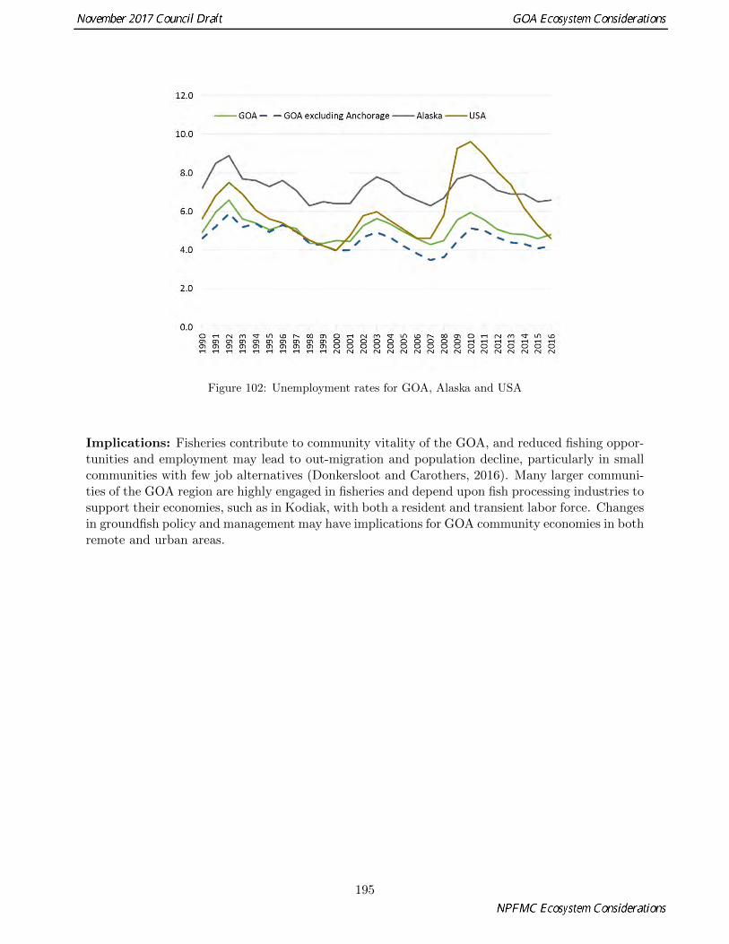
Figure 102: Unemployment rates for GOA, Alaska and USA

Implications: Fisheries contribute to community vitality of the GOA, and reduced fishing oppor-tunities and employment may lead to out-migration and population decline, particularly in smallcommunities with few job alternatives (Donkersloot and Carothers, 2016). Many larger communi-ties of the GOA region are highly engaged in fisheries and depend upon fish processing industries tosupport their economies, such as in Kodiak, with both a resident and transient labor force. Changesin groundfish policy and management may have implications for GOA community economies in bothremote and urban areas.

195

Socio-Cultural Dimensions

Trends in Human Population in the Gulf of Alaska

Contributed by Anna Lavoie, Resource Ecology and Fishery Management Division, Alaska Fish-eries Science Center, National Marine Fisheries Service, NOAAContact: [email protected] updated: September 2017

Description of indicator: Human population is a significant factor in the Gulf of Alaska (GOA)ecosystem, as many communities in the region rely upon fisheries to support their economies andto meet subsistence and cultural needs. As with areas neighboring the Arctic, population is animportant indicator of community viability (Rasmussen et al., 2015). Advancements in socio-ecological systems research have demonstrated the importance of incorporating social variables inecosystem management and monitoring (Turner et al., 2003; Ostrom, 2007). For example, variationin resource access or availability or employment opportunities may influence human migrationpatterns, which in turn may decrease human activity in one area of an ecosystem while increasingactivity in another.

This section summarizes trends in human population over time in the Gulf of Alaska (GOA) (includ-ing Southeast Alaska, Cook Inlet, and Prince William Sound). The 98 GOA fishing communitiesincluded in analysis comprise most of the population that resides along Gulf of Alaska coast. Com-munities were included if they are within 25 miles of the coast, and/or based on their historicalinvolvement in Gulf of Alaska fisheries, or if they were included in one of the North Pacific Fish-ery Management Councils GOA fishery programs, such as the Community Quota Entity program.Also, as of 2015 there was no population data for several communities that were previously includedin this report. They were not included in analysis because of insufficient data, however, they arementioned below. Population was calculated by summing community level data at decadal scalesfrom 1890–1990 (DCCED, 2016) and annually from 1990–2016 (ADLWD, 2017).

Status and trends: As of 2016 the population of GOA was 456,556 or 157,519 excluding Anchor-age. The population of small communities (population less than 1,500) was 26,000. The populationof all GOA communities has increased steadily since 1880 with the greatest population increase of194.2% occurring between 1950 and 1960 (Table 7). This figure includes Anchorage, the largestmajor city of Alaska, where the majority of population increase has occurred and where 40% ofAlaskas population currently resides (ADLWD2017a). With Anchorage excluded, and for smallcommunities, the greatest population increase of 50.2% occurred between 1980 and 1990 in theGOA (decadal increments). This is consistent with state trends as population change peaked dur-ing these periods (over 75% by 1960 and 36.9% by 1990). Population increase leveled off after 1990with lower rates in the following decades in the GOA and Alaska state. Between 1990 and 2016,the population of GOA increased 32.0% (31.8% excluding Anchorage) which is consistent with, yetlower than, state trends across this time period (34.5%)(Figure 103).

Despite the general population trend in the GOA as a whole, 41.2% of communities experiencedpopulation decline between 1990 and 2016. The communities of Hobart Bay, Annette, MeyersChuck and Cube Cove had no population data as of 2010. Communities of Ivanof Bay, Elfin Cove,Karluk, Pelican City, Point Baker, and Cold Bay also had decreases in population ranging from

196

Table 7: Gulf of Alaska (GOA) population 1880–2016. Percent change rates are decadal until 2010.

Year Alaska % change GOA % changeGOAexcludingAnchorage

GOA % changeexcludingAnchorage

1880 33,426 3,151 3,1511890 32,052 -4.11 7,469 137.04 7,469 137.041900 63,592 98.40 10,499 40.57 10,499 40.571910 64,356 1.20 13,394 27.57 13,394 27.571920 55,036 -14.48 17,208 28.48 15,352 14.621930 59,278 7.71 21,633 25.71 19,356 26.081940 72,524 22.35 29,213 35.04 25,718 32.871950 128,643 77.38 41,960 43.63 30,706 19.391960 226,167 75.81 123,456 194.22 40,623 32.301970 302,583 33.79 181,414 46.95 56,872 40.001980 401,851 32.81 253,961 39.99 79,530 39.841990 550,043 36.88 342,521 34.87 116,183 46.092000 626,932 13.98 400,222 16.85 139,939 20.452010 710,231 13.29 437,413 9.29 145,587 4.042016 739,828 4.17 456,556 2.98 157,519 3.96

Figure 103: Gulf of Alaska population 1990–2016. Anchorage is presented on the second (right) axis.

60.1% to 80.0%. In contrast, the community of Kalifornsky experience a population increase of

197

over 2,900% during this time period.

Indigenous Americans comprise up to 82% of the population of small communities in remote areas,and more Native Americans reside in Alaska than any U.S. state (Goldsmith et al., 2004). As of2014, 15% of Alaskas population was Alaska Native or Native American (ADLWD, 2016c), and asof 2015, 28% of the population in the GOA identified as Native American alone or combination withanother race (DCCED, 2016). In addition, there has been increased migration of Alaska Nativesfrom rural to urban areas (Goldsmith et al., 2004; Williams, 2004). The majority of populationgrowth that has occurred in Alaska and the GOA is of the Caucasian demographic (ADLWD,2016c).

Factors influencing observed trends: Overall population increase in GOA between 1990 and2016 (31.8%) was consistent with state trends (34.5%). Alaska has high rates of population turnoverbecause of migration, and population growth has occurred mainly in urban areas (ADLWD, 2016c).The main factors that affect population growth are natural increase (births minus deaths) andmigration, with the latter being the most unpredictable aspect of population change (Williams,2004; ADLWD, 2016c). In 2010, 61% of Alaskas population was born out of state (Rasmussen etal. 2015). In terms of natural growth, from 2010 to 2014 the average annual birth rate in Alaskawas 1.6 per 100 people which was higher than the national rate of 1.3 (ADLWD, 2016c). From2010–2014 the Aleutian chain and Southeast Alaska had the lowest natural increase (0.0–1.0%)whereas the Northern Bering Sea area had the highest (1.5–3.0%). The natural growth rates ofthe GOA had a range of 0.0–1.5% (ADLWD, 2016c). The the GOA region has the highest netmigration in the state, and the Matanuska-Susitna Borough has the highest growth rate (ADLWD,2016c).

Population trends in Alaska and the GOA region are the result of changes in resource extrac-tion and military activity (Williams, 2004). Historically, the gold rush of the late 19th centurydoubled the states population by 1900, and later WWII activity and oil development fueled thepopulation growth (ADLWD2016c). However, certain areas have experienced population shifts atvarious periods, particularly those with military bases. For example, the population of Kodiakdeclined in the 1990s because of Coast Guard cut-backs (Williams 2006). The fishing industryalso influences community population. Kodiak and the Aleutian Islands have the most transientpopulations because of the seafood processing industry (Williams, 2004). Some GOA communitiesthat experienced fishery permit loss subsequently experienced population decline (Donkersloot andCarothers, 2016). Also, reduction of jobs in the lumber industry have caused population decrease.For example, the Whitestone Logging Camp population fluctuated from 164 to 0 between 1990 and2006, increased to 17 in 2010 and was zero in subsequent years (ADLWD, 2017).

Implications: Population shifts can affect pressures on fisheries resources, however inferencesabout human impacts on resources should account for economic shifts and global market demand forseafood and other extractive resources of the ecoregion. As stated earlier, the majority of populationincreases in the GOA are due to increased net migration rather than natural increase, and they havemainly occurred in urban areas as populations in many small communities are declining. Fisheriescontribute to community vitality of the GOA. Reduced fishing opportunities and employmentmay lead to out-migration and population decline, particularly in small communities with few jobalternatives (Donkersloot and Carothers, 2016). Many larger communities of the GOA region arehighly engaged in fisheries and depend upon fish processing industries to support their economies,such as in Kodiak, with both a resident and transient labor force. Changes in groundfish policy andmanagement, such as increased regulations, may have implications for GOA community economies

198

in both remote and urban areas.

With a large concentration of Alaskas population in Anchorage, it has become the major hubfor goods and services, trade, and travel. Services such as medical, business and technology sup-port and entertainment attract people to the area seeking services, and employment and educa-tion opportunities. The population growth of Anchorage has also contributed to sprawl into theMatanuska-Susitna valley. According to the U.S. Census Bureau of 2010, the population density ofthe Matanuska-Susitna borough was 3.6, whereas the state as a whole was 1.2. This regional growthhas increased regional hunting and fishing pressures, recreational demand, and reduced availableagricultural land because of high speculative land values (Fischer, 1976). Rapid development ofthe Matanuska-Susitna valley may have impacts on the local watersheds fish stocks and habitat,which should be monitored over time.

Trends in School Enrollment in the Gulf of Alaska

Contributed by Sarah P. Wise1 and Kim Sparks21 Resource Ecology and Fishery Management Division, Alaska Fisheries Science Center, NationalMarine Fisheries Service, NOAA2 Resource Ecology and Fisheries Management Division, Alaska Fisheries Science Center, NationalMarine Fisheries Service, NOAA; and Alaska Fisheries Information Network, Pacific States MarineFisheries CommissionContact: [email protected] updated: September 2017

Description of indicator: Ensuring the productivity and sustainability of fishing communitiesis a core mandate of Federal fisheries management. One indicator to evaluate community vitalityis K-12 public school enrollment. Enrollments trends are of particular relevance due to the valueof schools to community cohesion and identity.

Public school enrollment was analyzed in the Gulf of Alaska (GOA) by borough and communitylevel in order to examine broader regional trends as well as the social and economic vitality ofindividual rural communities. Fishing communities were defined as in Lavoie p. 196. Enrollmentstatistics for K-12 grades by school and region were compiled for the years 1996–2014 from TheNational Center for Educational Statistics (https://nces.ed.gov/ccd/elsi/tableGenerator.aspx). More recent enrollment data were available for years 2014–2017 from the Alaska Departmentof Education and Early Development (http://www.eed.state.ak.us/stats/). Current schoollocations and names were verified using the EPA EJ mapping tool (https://ejscreen.epa.gov/mapper/). Municipalities or boroughs with enrollment over 4,500 were excluded from the analysisin order to avoid skewing the results (these included were the Matanuska-Susitna Borough, JuneauBorough, and Anchorage Municipality).

Status and trends: School enrollment patterns vary considerably in the GOA by rural and urbanareas and by population of the municipality. Within municipalities where school enrollment isover 500 students, school enrollment remains fairly stable, showing a general slight decrease inenrollment. Overall, there is a general decrease in enrollment. The exception to this is KenaiCity which has an increase in enrollment from 1424 students in 1996 to 1787 students in 2017, anincrease of 26 percent. In contrast school enrollment in Homer decreased nearly 50 percent among

199

https://nces.ed.gov/ccd/elsi/tableGenerator.aspx

https://nces.ed.gov/ccd/elsi/tableGenerator.aspx

http://www.eed.state.ak.us/stats/

https://ejscreen.epa.gov/mapper/

https://ejscreen.epa.gov/mapper/

those schools with over 500 students with 2302 students in 1996 and 1186 in currently (Figure 104).

Figure 104: GOA fishing community schools with enrollment over 500 students.

In municipalities with school enrollment between 100 and 500 students, there is a downward trendfor several schools including Hoonah City which decreased 60 percent, from 273 students to 109students since 1996, and Petersburg City and Angoon City, which both decreased 50% (Figure105).

Figure 105: GOA fishing community schools with enrollment between 500 and 100 students.

A majority of schools have enrollment under 100 students. Schools in smaller communities tendto have more variable enrollment trends. To illustrate, Figure 106 depicts Kodiak Island Borough

200

Table 8: GOA fishing community schools with enrollment of 30 or fewer students.

Status Previously open now closed ≤15 students 16–30 students

Numberof Schools

7 12 14

Cube Cove CDP Chenega CDP Chignik Lake CDPElfin Cove CDP Chignik city Coffman Cove cityEdna Bay city Chignik Lagoon CDP Cooper Landing CDPIvanof Bay CDP Hyder CDP Hope CDPMeyers Chuck CDP Karluk CDP Larsen Bay cityPort Protection CDP Kasaan city Tatitlek CDPTenakee Springs city Klukwan CDP Whale Pass CDP

Moose Pass CDP Tyonek CDPPelican city Old Harbor cityPerryville CDP Akhiok cityPort Alexander city Chiniak CDPPort Lions city Ouzinkie city

Hollis CDPNaukati Bay CDP

schools, with enrollments currently ranging from10 to 29. There is some fluctuation in enrollment,but an overall downward trend. Two schools dropped in enrollment forcing periodic school closures.The Karluk School first opened in 2001 with 10 students, closed in 2003, and re-opened in 2006with 10. Chiniak School closed in 2009 when enrollment dipped below the 10 student threshold,and re-opening in 2011. As of 2017, 27 schools have enrollment under 30, and 12 schools haveenrollments under 15 students (Table 8).

Figure 106: School enrollment in the Kodiak Island Borough.

Factors influencing observed trends: The GOA ecoregion varies substantially in populationand community structure and vitality. The GOA holds several larger municipalities, with largerschool enrollment, compared to other regions of Alaska. As people migrate to other areas, pop-ulations increase in adjacent communities. It is possible that enrollment may shift to the larger

201

communities as more convenient schools open. However other factors must be considered includingexisting infrastructure such as functional ports, airports, or medical facilities to provide supportfor a viable community structure. Those schools with enrollment under 30 students experience thegreatest uncertainty in terms of educational stability. With greater fluctuation in school enroll-ment, rural area schools are particularly vulnerable to closure and possible community disruption.The reasons for decreasing enrollment likely involve complex social and economic drivers includingmigratory patterns, resource availability, and employment. Additional research into the specific rea-sons for diminishing school enrollment in rural areas, as well as the impacts on these communitieswould inform and benefit management decisions.

Implications: Community residents are closely tied to the ecosystem through sense of place anddaily experience and activity. Schools are cultural centers and serve as important indicators of socialand economic viability, and community well-being (Lyson, 2002, 2005). Within rural communitiesin particular, schools are valuable symbols for community identity, autonomy, and shared socialvalues (Peshkin, 1978, 1982; Lyson, 2005). Research indicates that school closures negatively affectcommunities (Buzzard, 2016). Patterns of diminishing enrollment and school consolidation suggesta decrease in property values and taxes, fragmented community, and lost business, as well as declinesin reported quality of life scores (Sell and Leistritz, 1997; Lyson, 2002). Some research finds the rateof participation in community organizations decreases in communities experiencing school closures(Oncescu and Giles, 2014; Sell and Leistritz, 1997). These finding suggests that reduced enrollmentsand school closures may flag disruptions in social cohesion and viability, possibly leading to lessvibrant and sustainable communities.

202

References

Subsistence Fishing. http://www.adfg.alaska.gov. Accessed: 2017-10-10.

ADLWD. 2016a. Alaska Economic Trends. Employment Forecast 2016. Alaska Department ofLabor and Workforce Development. January 2016, Volume 36, No. 1. Report.

ADLWD. 2016b. Alaska Economic Trends. Is Alaska in a Recession? Alaska Department of Laborand Workforce Development. February 2016, Volume 36, No. 2. Report.

ADLWD. 2016c. Alaska Population Overview: 2015 Estimates. Report, Alaska Department ofLabor and Workforce Development.

ADLWD. 2017. Cities and Census Designated Places (CDPs), 2010 to 2016. Report, AlaskaDepartment of Labor and Workforce Development.

AFSC. 2011. Observer Sampling Manual for 2012. Technical report, Alaska Fisheries Science Center,Fisheries Monitoring and Analysis Division, North Pacific Groundfish Observer Program, 7600Sand Point Way, NE.; Seattle WA; 98115.

Anderson, P. J. 2003. Gulf of Alaska small mesh trawl survey trends, In: J.L.Boldt (Ed.), EcosystemConsiderations for 2004. Appendix C of the BSAI/GOA Stock Assessment and Fishery EvaluationReports. Technical report, North Pacific Fishery Management Council, 605 W. 4th Ave., Suite306, Anchorage, AK 99501.

Atwood, E., J. K. Duffy-Anderson, J. K. Horne, and C. Ladd. 2010. Influence of mesoscale eddieson ichthyoplankton assemblages in the Gulf of Alaska. Fisheries Oceanography 19:493–507.

Batten, S. D., and D. W. Welch. 2004. Changes in oceanic zooplankton populations in the north-east Pacific associated with the possible climatic regime shift of 1998/1999. Deep Sea ResearchPart II: Topical Studies in Oceanography 51:863–873.

Beamish, R. J., C. Neville, R. Sweeting, and K. Lange. 2012. The Synchronous Failure of JuvenilePacific Salmon and Herring Production in the Strait of Georgia in 2007 and the Poor Return ofSockeye Salmon to the Fraser River in 2009. Marine and Coastal Fisheries 4:403–414.

Beamish, R. J., R. M. Sweeting, and C. M. Neville. 2004. Improvement of Juvenile Pacific SalmonProduction in a Regional Ecosystem after the 1998 Climatic Regime Shift. Transactions of theAmerican Fisheries Society 133:1163–1175.

Boldt, J. L., and L. J. Haldorson. 2004. Size and condition of wild and hatchery pink salmonjuveniles in Prince William Sound, Alaska. Transactions of the American Fisheries Society133:173–184.

203

http://www.adfg.alaska.gov

Bond, N. A., M. F. Cronin, H. Freeland, and N. Mantua. 2015. Causes and impacts of the 2014warm anomaly in the NE Pacific. Geophysical Research Letters 42:3414–3420.

Bond, N. A., and L. Guy. 2010. North Pacific Climate Overview In: S. Zador and S. Gaichas(Ed.), Ecosystem Considerations for 2010. Appendix C of the BSAI/GOA Stock Assessment andFishery Evaluation Report. Technical report, North Pacific Fishery Management Council, 605W. 4th Ave., Suite 306, Anchorage, AK 99501.

Bradford, A. L., D. W. Weller, A. E. Punt, Y. V. Ivashchenko, A. M. Burdin, G. R. VanBlari-com, and R. L. Brownell Jr. 2012. Leaner leviathans: body condition variation in a criticallyendangered whale population. Journal of Mammalogy 93:251–266.

Brickley, P. J., and A. C. Thomas. 2004. Satellite-measured seasonal and inter-annual chlorophyllvariability in the Northeast Pacific and Coastal Gulf of Alaska. Deep-Sea Research Part Ii-TopicalStudies in Oceanography 51:229–245.

Brodeur, R., and D. M. Ware. 1992. Long-term variability in zooplankton biomass in the subarcticPacific Ocean. Fisheries Oceanography 1:32–37.

Brodeur, R. D., M. B. Decker, L. Ciannelli, J. E. Purcell, N. A. Bond, P. J. Stabeno, E. Acuna,and G. L. Hunt. 2008. Rise and fall of jellyfish in the eastern Bering Sea in relation to climateregime shifts. Progress in Oceanography 77:103–111.

Brodeur, R. D., R. L. Emmett, J. P. Fisher, E. Casillas, D. J. Teel, and T. W. Miller. 2004. Juvenilesalmonid distribution, growth, condition, origin, and environmental and species associations inthe Northern California Current. Fishery Bulletin 102:25–46.

Buckley, T. W., A. Greig, and J. L. Boldt. 2009. Describing summer pelagic habitat over thecontinental shelf in the eastern Bering Sea, 1982-2006. Report.

Buzzard, R. A. 2016. What Every Policy Maker, School Leader, Parent, and Community MemberNeeds to Know About the Social, Economic, and Human Capital Costs of Closing a Rural School:A Comprehensive Multi-faceted Investigation. Niagara University.

Cahalan, J., J. Mondragon, and J. Gasper. 2010. Catch sampling and estimation in the Federalgroundfish fisheries off Alaska. Technical report, U.S. Dep. Commer., NOA Tech. Memo. NMFS-AFSC-205, 42 p.

Cahalan, J. A., J. R. Gasper, and J. Mondragon. 2014. Catch Sampling and Estimation in theFederal Groundfish Fisheries off Alaska, 2015 Edition. Report, US Department of Commerce,National Oceanic and Atmospheric Administration, National Marine Fisheries Service, AlaskaFisheries Science Center.

Calambokidis, J., E. A. Falcone, T. J. Quinn, A. M. Burdin, P. Clapham, J. Ford, C. Gabriele,R. LeDuc, D. Mattila, and L. Rojas-Bracho. 2008. SPLASH: Structure of populations, levels ofabundance and status of humpback whales in the North Pacific. Report.

Combes, V., and E. Di Lorenzo. 2007. Intrinsic and forced interannual variability of the Gulf ofAlaska mesoscale circulation. Progress in Oceanography 75:266–286.

Condon, R. H., D. K. Steinberg, P. A. del Giorgio, T. C. Bouvier, D. A. Bronk, W. M. Graham,and H. W. Ducklow. 2011. Jellyfish blooms result in a major microbial respiratory sink of carbonin marine systems. Proceedings of the National Academy of Sciences 108:10225–10230.

204

Coyle, K. O., L. Eisner, F. J. Mueter, A. Pinchuk, M. Janout, K. Cieciel, E. Farley, and A. Andrews.2011. Climate change in the southeastern Bering Sea: impacts on pollock stocks and implicationsfor the Oscillating Control Hypothesis. Fisheries Oceanography 20:139–156.

Coyle, K. O., A. Pinchuk, L. Eisner, and J. M. Napp. 2008. Zooplankton species composition,abundance and biomass on the eastern Bering Sea shelf during summer: the potential role of watercolumn stability and nutrients in structuring the zooplankton community. Deep-Sea ResearchPart II 55:1755–1791.

Coyle, K. O., and A. I. Pinchuk. 2003. Annual cycle of zooplankton abundance, biomass andproduction on the northern Gulf of Alaska shelf, October 1997 through October 2000. FisheriesOceanography 12:327–338.

Dahlheim, M. E., P. A. White, and J. M. Waite. 2009. Cetaceans of Southeast Alaska: distributionand seasonal occurrence. Journal of Biogeography 36:410–426.

DCCED. 2016. State of Alaska Department of Commerce, Community and Economic Devel-opment. Community and Regional Analysis, Community Database Online. Report. https:

//www.commerce.alaska.gov/dcra/DCRAExternal

Di Lorenzo, E., D. Mountain, H. Batchelder, N. Bond, and E. Hofmann. 2013. Advances in marineecosystem dynamics from US GLOBEC: The horizontal-advection bottom-up forcing paradigm.Oceanography 26:2233.

Dietrich, K. S., and E. F. Melvin. 2008. Alaska Trawl Fisheries: Potential Interations with NorthPacific Albatrosses. Technical report, Washington Sea Grant.

Donkersloot, R., and C. Carothers. 2016. The graying of the Alaskan fishing fleet. Environment:Science and Policy for Sustainable Development 58:30–42.

Dougherty, A. 2015. Gulf of Alaska: Too warm for larval walleye pollock survival in 2015? In: Zador,S.G., (Ed.), Ecosystem Considerations 2015: Status of Alaska’s Marine Ecosystems. Techincalreport, North Pacific Fishery Management Council, 605 W 4th Ave, Suite 306, Anchorage, AK99501.

Doyle, M. J., S. J. Picquelle, K. L. Mier, M. Spillane, and N. bond. 2009. Larval fish abundanceand physical forcing in the Gulf of Alaska, 1981-2003. Progress in Oceanography 80:163–187.

Ducet, N., P. Y. Le Traon, and G. Reverdin. 2000. Global high-resolution mapping of oceancirculation from TOPEX/Poseidon and ERS-1 and-2. Journal of Geophysical Research-Oceans105:19477–19498.

Fall, J. A., L. B. Hutchinson-Scarbrough, B. Jones, D. Kukkonen, D. Runfola, L. A. Still, andT. Lemons. 2017. Alaska subsistence and personal use salmon fisheries 2014 annual report.Report, Alaska Department of Fish and Game, Division of Subsistence.

Fall, J. A., and T. Lemons. 2015. Subsistence harvests of Pacific halibut in Alaska, 2014. Report.

Fall, J. A., and T. Lemons. 2016. Presentation B3 Subsistence Halibut Harvests. Report.

Fergusson, E. A., M. V. Sturdevant, and J. A. Orsi. 2013. Trophic relationships among juvenilesalmon during a 16-year time series of climate variability in Southeast Alaska. Technical report.

205

https://www.commerce.alaska.gov/dcra/DCRAExternal

https://www.commerce.alaska.gov/dcra/DCRAExternal

Fischer, V. 1976. Regional effects of Anchorage metropolitan growth. Fairbanks: Institute of Social,Economic and Government Research, University of Alaska.

Fissel, B., M. Dalton, R. Felthoven, B. Garber-Yonts, A. Haynie, A. Himes-Cornell, S. Kasperski,J. Lee, D. Lew, and C. Seung. 2016. Stock assessment and fishery evaluation report for thegroundfish fisheries of the Gulf of Alaska and Bering Sea/Aleutian Islands area: economic statusof the groundfish fisheries off Alaska, 2015. Report.

Fritz, L. W., K. Sweeney, R. G. Towell, and T. W. Gelatt. 2016. Aerial and ship-based surveys ofSteller sea lions (Eumetopias jubatus) conducted in Alaska in June-July 2013 through 2015, andan update on the status and trend of the western distinct population segment in Alaska. Report.

Fuentes, M. M., S. Delean, J. Grayson, S. Lavender, M. Logan, and H. Marsh. 2016. Spatial andTemporal Variation in the Effects of Climatic Variables on Dugong Calf Production. PloS one11:e0155675.

Gabriele, C. M., J. L. Neilson, J. M. Straley, C. S. Baker, J. A. Cedarleaf, and J. F. Saracco. 2017.Natural history, population dynamics, and habitat use of humpback whales over 30 years on anAlaska feeding ground. Ecosphere 8.

Gilroy, H. L. The Pacific halibut fishery, 2004. in International Pacific Halibut Commission Eighty-First Annual Meeting, page 1907 .

Goldsmith, S., J. Angvik, L. Howe, A. Hill, and L. Leask. 2004. The Status of Alaska NativesReport. I. Anchorage: Institute of Social and Economic Research, University of Alaska.

Greene, K. 2002. Coastal cool-down. Science 295:1823–1823.

Grenier, C. 2014. Quantifying Ichthyophonus prevalence and load in Pacific halibut (Hippoglossusstenolepsis) in Cook Inlet, Alaska. Master’s.

Guthrie III, C., H. T. Nguyen, A. E. Thomson, and J. Guyon. 2017. Genetic stock compositionanalysis of the Chinook salmon bycatch from the 2015 Gulf of Alaska trawl fisheries. Report.

Hanselman, D., C. Lunsford, and C. Rodgveller. 2013. Assessment of the sablefish stock in Alaska.Technical report, North Pacific Fishery Management Council.

Hanselman, D., C. Lunsford, C. Rodgveller, and M. J. Peterson. 2016. Assessment of the Sable-fish stock in Alaska, Stock Assessment and Fishery Evaluation Report, North Pacific FisheryManagement Council, 605 W 4th Ave, Suite 306, Anchorage, AK 99501. Report.

Harris, B. P., S. R. Webster, N. Wolf, J. L. Gregg, and P. K. Hershberger. InReview. Ichthyophonusin Southcentral Alaska Groundfish. Journal of Aquatic Animal Health .

Harris, R., P. Wiebe, L. J., S. H.R., and H. M. 2005. ICES Zooplankton Methodology Manual.Elsevier Academic Press, Amsterdam.

Hatch, S. A. 2013. Kittiwake diets and chick production signal a 2008 regime shift in the NortheastPacific. Marine Ecology Progress Series 477:271–284.

Heard, W. R. 2009. Alaska Salmon. Unit 13 in Our Living Oceans, 6th edition. Report.

Hebert, K. P. 2017. Southeast Alaska 2016 herring stock assessment surveys. Report, AlaskaDepartment of Fish and Game, Fishery Data Series No. 17-01.

206

Hendrix, A., J. Straley, C. Gabriele, and S. Gende. 2012. Bayesian estimation of humpback whale(Megaptera novaeangliae) population abundance and movement patterns in southeastern Alaska.Canadian Journal of Fisheries and Aquatic Sciences 69:1783–1797.

Hunt, G. L., P. H. Ressler, G. A. Gibson, A. De Robertis, K. Aydin, M. F. Sigler, I. Ortiz, E. J.Lessard, B. C. Williams, and A. Pinchuk. 2016. Euphausiids in the eastern Bering Sea: Asynthesis of recent studies of euphausiid production, consumption and population control. DeepSea Research Part II: Topical Studies in Oceanography 134:204–222.

Ianelli, J. N., T. Honkalehto, S. Barbeaux, S. Kotwicki, K. Y. Aydin, and N. Williamson. 2012.Assessment of the walleye pollock stock in the Eastern Bering Sea. Technical report, N Pac FishManage Council, 605 W 4th Ave, Anchorage, AK 99510.

Jennings, G. B., K. Sundet, and A. E. Bingham. 2015. Estimates of participation, catch, andharvest in Alaska sport fisheries during 2011. Report.

Kelleher, K. 2005. Discards in the world’s marine fisheries: an update. Food & Agriculture Org.

King, J. 2005. Report of the Study Group on Fisheries and Ecosystem Responses to recent regimeshifts. PICES Scientific Report No. 28. Technical report.

Kline, J., T. C. 2010. Stable carbon and nitrogen isotope variation in the northern lampfish andNeocalanus, marine survival rates of pink salmon, and meso-scale eddies in the Gulf of Alaska.Progress in Oceanography 87:49–60.

Kotwicki, S., and R. R. Lauth. 2013. Detecting temporal trends and environmentally-driven changesin the spatial distribution of bottom fishes and crabs on the eastern Bering Sea shelf. Deep SeaResearch Part II: Topical Studies in Oceanography 94:231–243.

Kovach, R. P., J. E. Joyce, J. D. Echave, M. S. Lindberg, and D. A. Tallmon. 2013. EarlierMigration Timing, Decreasing Phenotypic Variation, and Biocomplexity in Multiple SalmonidSpecies. PLoS ONE 8:e53807.

Ladd, C. 2007. Interannual variability of the Gulf of Alaska eddy field. Geophysical ResearchLetters 34.

Ladd, C., and W. Cheng. 2016. Gap winds and their effects on regional oceanography Part I: CrossSound, Alaska. Deep Sea Research II .

Ladd, C., W. R. Crawford, C. Harpold, W. Johnson, N. B. Kachel, P. Stabeno, and F. Whitney.2009. A synoptic survey of young mesoscale eddies in the Eastern Gulf of Alaska. Deep-SeaResearch Part II 56:2460–2473.

Ladd, C., N. B. Kachel, C. W. Mordy, and P. J. Stabeno. 2005. Observations from a Yakutat eddyin the northern Gulf of Alaska. Journal of Geophysical Research-Oceans 110.

Ladd, C., C. W. Mordy, N. B. Kachel, and P. J. Stabeno. 2007. Northern Gulf of Alaska eddies andassociated anomalies. Deep-Sea Research Part I-Oceanographic Research Papers 54:487–509.

Landingham, J. H., M. V. Sturdevant, and R. D. Brodeur. 1998. Feeding habits of juvenile Pacificsalmon in marine waters of southeastern Alaska and northern British Columbia. Fishery Bulletin96:285–302.

207

Lew, D. K., and D. M. Larson. 2011. A repeated mixed logit approach to valuing a local sportfishery: the case of Southeast Alaska salmon. Land Economics 87:712–729.

Lew, D. K., and D. M. Larson. 2012. Economic values for saltwater sport fishing in Alaska: Astated preference analysis. North American journal of fisheries management 32:745–759.

Lew, D. K., and D. M. Larson. 2015. Stated preferences for size and bag limits of Alaska charterboat anglers. Marine Policy 61:66–76.

Li, K., A. J. Doubleday, M. D. Galbraith, and R. R. Hopcroft. 2016. High abundance of salps inthe coastal Gulf of Alaska during 2011: A first record of bloom occurrence for the northern Gulf.Deep Sea Research Part II: Topical Studies in Oceanography 132:136–145.

Link, J. S., J. K. T. Brodziak, S. F. Edwards, W. J. Overholtz, D. Mountain, J. W. Jossi, T. D.Smith, and M. J. Fogarty. 2002. Marine ecosystem assessment in a fisheries management context.Canadian Journal of Fisheries and Aquatic Sciences 59:1429–1440.

Loring, P. A., and S. C. Gerlach. 2009. Food, culture, and human health in Alaska: an integrativehealth approach to food security. Environmental Science & Policy 12:466–478.

Lovell, S. J., S. Steinback, and J. Hilger. 2013. The Economic Contribution of Marine AnglerExpenditures in the United States. Report.

Lyson, T. 2005. The importance of schools to rural community viability. A Mathematics EducatorsIntroduction to Rural Policy Issues 48.

Lyson, T. A. 2002. What Does a School Mean to a Community? Assessing the Social and EconomicBenefits of Schools to Rural Villages in New York .

Mackas, D. L., W. Greve, M. Edwards, S. Chiba, K. Tadokoro, D. Eloire, M. G. Mazzocchi,S. Batten, A. J. Richardson, C. Johnson, E. Head, A. Conversi, and T. Peluso. 2012. Changingzooplankton seasonality in a changing ocean: Comparing time series of zooplankton phenology.Progress in Oceanography 97100:31–62.

Mackas, D. L., W. T. Peterson, and J. E. Zamon. 2004. Comparisons of interannual biomassanomalies of zooplankton communities along the continental margins of British Columbia andOregon. Deep Sea Research Part II: Topical Studies in Oceanography 51:875–896.

Magurran, A. E. 1988. Ecological diversity and its measurement. Princeton University Press,Princeton, N.J.

McCann, K. S. 2000. The diversitystability debate. Nature 405:228–233.

Meyer, S. 2010. Changes coming for Alaska’s charter halibut fishery. Report.

Moran, J., R. Heintz, J. Straley, and J. Vollenweider. 2017. Regional variation in the intensity ofhumpback whale predation on Pacific herring in the Gulf of Alaska. Deep Sea Research Part II:Topical Studies in Oceanography .

Mueter, F. J., R. M. Peterman, and B. J. Pyper. 2002. Opposite effects of ocean temperatureon survival rates of 120 stocks of Pacific salmon (Oncorhynchus spp.) in northern and southernareas. Canadian Journal of Fisheries and Aquatic Sciences 59:456–463.

208

Mundy, P. R. 2005. The Gulf of Alaska: biology and oceanography. Alaska Sea Grant CollegeProgram.

Muto, M., V. Helker, R. Angliss, B. Allen, P. Boveng, J. Breiwick, M. Cameron, P. Clapham,S. Dahle, M. Dahlheim, B. S. Fadely, M. C. Ferguson, L. W. Fritz, R. C. Hobbs, Y. V.Ivashchenko, A. S. Kennedy, J. M. London, S. A. Mizroch, R. R. Ream, E. L. Richmond, K. E. W.Shelden, R. G. Towell, P. R. Wade, J. N. Waite, and A. N. Zerbini. Alaska Marine MammalStock Assessments, 2016 page 366 .

Neilson, J. L., and C. M. Gabriele. 2016. Results of humpback whale monitoring in Glacier Bayand adjacent waters 2015: Annual progress report. Report.

Neilson, J. L., C. M. Gabriele, and L. F. Taylor-Thomas. 2017. Humpback whale monitoring inGlacier Bay and adjacent waters 2016: Annual progress report. Report.

Neilson, J. L., C. M. Gabriele, and P. B. S. Vanselow. 2015. Results of humpback whale monitoringin Glacier Bay and adjacent waters 2014: Annual progress report. Report.

Okkonen, S. R., G. A. Jacobs, E. J. Metzger, H. E. Hurlburt, and J. F. Shriver. 2001. Mesoscalevariability in the boundary currents of the Alaska Gyre. Continental Shelf Research 21:1219–1236.

Okkonen, S. R., T. J. Weingartner, S. L. Danielson, D. L. Musgrave, and G. M. Schmidt. 2003.Satellite and hydrographic observations of eddy-induced shelf-slope exchange in the northwesternGulf of Alaska. Journal of Geophysical Research-Oceans 108.

Oncescu, J. M., and A. Giles. 2014. Rebuilding a sense of community through reconnection: Theimpact of a rural school’s closure on individuals without school-aged children. Journal of Ruraland Community Development 9.

Orsi, J., A. Wertheimer, M. Sturdevant, E. Fergusson, D. Mortensen, and B. Wing. 2004. Juvenilechum salmon consumption of zooplankton in marine waters of southeastern Alaska: a bioen-ergetics approach to implications of hatchery stock interactions. Reviews in Fish Biology andFisheries 14:335–359.

Orsi, J. A., E. A. Fergusson, E. M. Yasumiishi, E. V. Farley, and R. A. Heintz. 2015. SoutheastAlaska Coastal Monitoring (SCEM) survey plan for 2015. Technical report, Auke Bay Lab.,Alaska Fisheries Science Center, NOAA, NMFS.

Orsi, J. A., A. Piston, E. A. Fergusson, and J. Joyce. 2014. Biological monitoring of key salmonpopulations: Southeast Alaska pink salmon. Technical report.

Ostrom, E. 2007. A diagnostic approach for going beyond panaceas. Proceedings of the nationalAcademy of sciences 104:15181–15187.

Park, W., M. V. Sturdevant, J. A. Orsi, A. Wertheimer, E. A. Fergusson, W. R. Heard, andT. Shirley. 2004. Interannual abundance patterns of copepods during an ENSO event in IcyStrait, southeastern Alaska. Ices Journal of Marine Science 61:464–477.

Paul, J. M., A. Paul, and W. E. Barber. 1997. Reproductive biology and distribution of the snowcrab from the northeastern Chukchi Sea, pages 287–294 . Bethesda, MD.

Peshkin, A. 1978. Growing Up American; Schooling and the Survival of Community .

209

Peshkin, A. 1982. The Imperfect Union. School Consolidation & Community Conflict. ERIC.

Peterson, G. D., S. R. Carpenter, and W. A. Brock. 2003. Uncertainty and the management ofmultistate ecosystems: an apparently rational route to collapse. Ecology 84:1403–1411.

Petitgas, P. 1993. Geostatistics for fish stock assessments: a review and an acoustic application.ICES Journal of Marine Science: Journal du Conseil 50:285–298.

Piatt, J. F., and P. J. Anderson. 1996. Response of Common Murres to the Exxon Valdez oilspill and long-term changes in the Gulf of Alaska marine ecosystem. American Fisheries SocietySymposium 18:720–737.

Picou, J. S., D. A. Gill, C. L. Dyer, and E. W. Curry. 1992. Disruption and stress in an Alaskanfishing community: Initial and continuing impacts of the Exxon Valdez oil spill. Industrial CrisisQuarterly 6:235–257.

Pierszalowski, S. P., C. M. Gabriele, D. J. Steel, J. L. Neilson, P. B. Vanselow, J. A. Cedarleaf,J. M. Straley, and C. S. Baker. 2016. Local recruitment of humpback whales in Glacier Bay andIcy Strait, Alaska, over 30 years. Endangered Species Research 31:177–189.

Piston, A., and S. Heinl. 2014. Pink salmon stock status and escapement goals in southeast Alaska.Technical report, Alaska Department of Fish and Game.

Purcell, J. E. 2005. Climate effects on formation of jellyfish and ctenophore blooms: a review.Journal of the Marine Biological Association of the United Kingdom 85:461–476.

Purcell, J. E., and M. N. Arai. 2001. Interactions of pelagic cnidarians and ctenophores with fish:a review. Hydrobiologia 451:27–44.

Purcell, J. E., R. A. Hoover, and N. T. Schwarck. 2009. Interannual variation of strobilationby the scyphozoan Aurelia labiata in relation to polyp density, temperature, salinity, and lightconditions in situ. Marine Ecology Progress Series 375:139–149.

Purcell, J. E., and M. V. Sturdevant. 2001. Prey selection and dietary overlap among zooplank-tivorous jellyfish and juvenile fishes in Prince William Sound, Alaska. Marine Ecology ProgressSeries 210:67–83.

Rasmussen, R. E., G. K. Hovelsrud, and S. Gearheard. 2015. Community Viability. Nordic Councilof Ministers.

Ream, R. R., J. T. Sterling, and T. R. Loughlin. 2005. Oceanographic features related to northernfur seal migratory movements. Deep-Sea Research Part Ii-Topical Studies in Oceanography52:823–843.

Ressler, P., A. De Robertis, and S. Kotwicki. 2014. The spatial distribution of euphausiids andwalleye pollock in the eastern Bering Sea does not imply top-down control by predation. MarineEcology Progress Series 503:111–122.

Ressler, P. H., A. De Robertis, J. D. Warren, J. N. Smith, and S. Kotwicki. 2012. Developing anacoustic survey of euphausiids to understand trophic interactions in the Bering Sea ecosystem.Deep Sea Research Part II: Topical Studies in Oceanography 6570:184–195.

210

Richardson, A. J., A. Bakun, G. C. Hays, and M. J. Gibbons. 2009. The jellyfish joyride: causes,consequences and management responses to a more gelatinous future. Trends in ecology &evolution 24:312–322.

Richardson, A. J., A. W. Walne, A. G. J. John, T. D. Jonas, J. A. Lindley, D. W. Sims, D. Stevens,and M. Witt. 2006. Using continuous plankton recorder data. Progress in Oceanography 68:27–74.

Robinson, K. L., J. J. Ruzicka, and M. B. Decker. 2014. Jellyfish, Forage Fish, and the WorldsMajor Fisheries .

Rogers, L. A., and K. L. Mier. 2016. Gulf of Alaska Ichthyoplankton Abundance Indices 1981-2015. In: Zador, S. G., and Yasumiishi, E. M. (Eds.), Ecosystem Considerations 2015: Status ofAlaska’s Marine Ecosystems. Technical report, North Pacific Fishery Management Council, 605W 4th Ave, Suite 306, Anchorage, AK 99501.

Romberg, W. J. 2016. Alaska Statewide Sport Fish Harvest Survey, 2016. Alaska Department ofFish and Game, Regional Operational Plan SF.4A.2016.04,, Anchorage.

Rooney, S., E. A. Laman, C. Rooper, K. Turner, D. W. Cooper, and M. Zimmermann. in press.Model-based essential fish habitat definitions for Gulf of Alaska groundfish species .

Rooper, C. N. 2008. An ecological analysis of rockfish (Sebastes spp.) assemblages in the NorthPacific Ocean along broad-scale environmental gradients. Fishery Bulletin 106:1–11.

Scannell, H. A., A. J. Pershing, M. A. Alexander, A. C. Thomas, and K. E. Mills. 2016. Frequencyof marine heatwaves in the North Atlantic and North Pacific since 1950. Geophysical ResearchLetters 43:2069–2076.

Schnaittacher, G. M., and R. E. Narita. 2013. Incidental catches of salmonids by US groundfishfisheries in the Bering Sea/Aleutian Islands and the Gulf of Alaska, 1990-2012. NPAFC Doc1476.

Sell, R. S., and F. L. Leistritz. 1997. Socioeconomic impacts of school consolidation on host andvacated communities. Community Development 28:186–205.

Seyboth, E., K. R. Groch, L. Dalla Rosa, K. Reid, P. A. Flores, and E. R. Secchi. 2016. Southernright whale (Eubalaena australis) reproductive success is influenced by krill (Euphausia superba)density and climate. Scientific reports 6:28205.

Shanley, C. S., S. Pyare, M. I. Goldstein, P. B. Alaback, D. M. Albert, C. M. Beier, T. J. Brinkman,R. T. Edwards, E. Hood, and A. MacKinnon. 2015. Climate change implications in the northerncoastal temperate rainforest of North America. Climatic Change 130:155–170.

Sigler, M., D. Tollit, J. J. Vollenweider, J. F. Thedinga, D. J. Csepp, J. N. Womble, M. A. Wong,M. J. Rehberg, and A. W. Trites. 2009. Steller Sea Lion Foraging Response to Seasonal Changesin Prey Availability. Marine Ecology Progress Series 388.

Sigler, M., and H. H. Zenger Jr. 1989. Assessment of Gulf of Alaska sablefish and other groundfishbased on the domestic longline survey, 1987. Technical report, U.S. Department of Commerce,NOAA Technical Memo.

211

Simonsen, K., P. H. Ressler, C. Rooper, and S. Zador. 2016. Spatio-temporal distribution ofeuphausiids: an important component to understanding ecosystem processes in the Gulf of Alaskaand eastern Bering Sea. ICES Journal of Marine Science 73:2020–2036.

Sousa, L., K. O. Coyle, R. P. Barry, T. J. Weingartner, and R. R. Hopcroft. 2016. Climate-relatedvariability in abundance of mesozooplankton in the northern Gulf of Alaska 19982009. Deep SeaResearch Part II: Topical Studies in Oceanography .

Straley, J. M., J. R. Moran, K. M. Boswell, J. J. Vollenweider, R. A. Heintz, T. J. Quinn II, B. H.Witteveen, and S. D. Rice. 2017. Seasonal presence and potential influence of humpback whaleson wintering Pacific herring populations in the Gulf of Alaska. Deep Sea Research Part II: TopicalStudies in Oceanography .

Straley, J. M., I. Quinn, J. Terrance, and C. M. Gabriele. 2009. Assessment of markrecapture modelsto estimate the abundance of a humpback whale feeding aggregation in Southeast Alaska. Journalof biogeography 36:427–438.

Stram, D. L., and J. N. Ianelli. 2014. Evaluating the efficacy of salmon bycatch measures usingfishery-dependent data. ICES Journal of Marine Science 72:1173–1180.

Sturdevant, M., M. Sigler, and J. Orsi. 2009. Sablefish predation on juvenile Pacific salmon inthe coastal marine waters of Southeast Alaska in 1999. Transactions of the American FisheriesSociety 138:675–691.

Sturdevant, M. V., J. A. Orsi, and E. A. Fergusson. 2012. Diets and Trophic Linkages of EpipelagicFish Predators in Coastal Southeast Alaska during a Period of Warm and Cold Climate Years,19972011. Marine and Coastal Fisheries 4:526–545.

Thorson, J. T., and K. Kristensen. 2016. Implementing a generic method for bias correction instatistical models using random effects, with spatial and population dynamics examples. FisheriesResearch 175:66–74.

Thorson, J. T., M. L. Pinsky, and E. J. Ward. 2016a. Model-based inference for estimating shiftsin species distribution, area occupied and centre of gravity. Methods in Ecology and Evolution7:990–1002.

Thorson, J. T., A. Rindorf, J. Gao, D. H. Hanselman, and H. Winker. 2016b. Density-dependentchanges in effective area occupied for sea-bottom-associated marine fishes 283:20161853.

Thorson, J. T., A. O. Shelton, E. J. Ward, and H. J. Skaug. 2015. Geostatistical delta-generalizedlinear mixed models improve precision for estimated abundance indices for West Coast ground-fishes. ICES Journal of Marine Science 72:1297–1310.

Turner, B. L., R. E. Kasperson, P. A. Matson, J. J. McCarthy, R. W. Corell, L. Christensen,N. Eckley, J. X. Kasperson, A. Luers, and M. L. Martello. 2003. A framework for vulnerabilityanalysis in sustainability science. Proceedings of the national academy of sciences 100:8074–8079.

Weitkamp, L. A., J. A. Orsi, K. Myers, and R. Francis. 2011. Contrasting early marine ecologyof Chinook salmon and coho salmon in Southeast Alaska: insight into factors affecting marinesurvival. Marine and Coastal Fisheries 3:233–249.

212

Wertheimer, A. C., J. A. Orsi, and E. A. Fergusson. 2015. Forecasting pink salmon harvest insoutheast Alaska from juvenile salmon abundance and associated biophysical parameters: 2014returns and 2015 forecast. Report.

Wespestad, V. G., L. W. Fritz, W. J. Ingraham, and B. A. Megrey. 2000. On relationships betweencannibalism, climate variability, physical transport, and recruitment success of Bering Sea walleyepollock (Theragra chalcogramma). Ices Journal of Marine Science 57:272–278.

Wilderbuer, T. K., A. B. Hollowed, W. J. Ingraham, P. D. Spencer, M. E. Conners, N. A. Bond,and G. E. Walters. 2002. Flatfish recruitment response to decadal climatic variability and oceanconditions in the eastern Bering Sea. Progress in Oceanography 55:235–247.

Williams, J. G. 2004. Alaska Population Overview: 2003-2004 Estimates. Technical report, TheState of Alaska Department of Labor and Workforce Development, Research and Analysis Sec-tion, Demographics Unit.

Yasumiishi, E. M., S. K. Shotwell, D. H. Hanselman, J. A. Orsi, and E. A. Fergusson. 2015.Using Salmon Survey and Commercial Fishery Data to Index Nearshore Rearing Conditions andRecruitment of Alaskan Sablefish. Marine and Coastal Fisheries 7:316–324.

213

ecosystem considerations 2017 · mayumi arimitsu, sonia batten, jennifer boldt, nick bond, jennifer...

Documents