MPRAMunich Personal RePEc Archive

Economies of Scale in the Canadian FoodProcessing Industry

Jean-Philippe Gervais and Olivier Bonroy and Steve Couture

August 2006

Online at https://mpra.ub.uni-muenchen.de/64/MPRA Paper No. 64, posted 3 October 2006

Economies of Scale in the Canadian Food Processing Industry

Jean-Philippe Gervais* Olivier Bonroy Steve Couture

August 2006

Abstract: Cost functions for three Canadian manufacturing agri-food sectors (meat, bakery and dairy) are estimated using provincial data from 1990 to 1999. A translog functional form is used and the concavity property is imposed locally. The Morishima substitution elasticities and returns to scale elasticities are computed for different provinces. Inference is carried out using asymptotic theory as well as bootstrap methods. In particular, the ability of the double bootstrap to provide refinements in inference is investigated. The evidence suggests that there are significant substitution possibilities between the agricultural input and other production factors in the meat and bakery sectors. Scale elasticity parameters indicate that increasing returns to scale are present in small bakery industries. While point estimates suggest that increasing returns to scale exist at the industry level in the meat sector, statistical inference cannot rule the existence of decreasing returns to scale. To account for supply management in the dairy sector, separability between raw milk and the other inputs was introduced. There exists evidence of increasing returns to scale at the industry level in the dairy industries of Alberta and New Brunswick. The scale elasticity for the two largest provinces (Ontario and Quebec) is greater than one, but inference does not reject the null hypothesis of increasing returns to scale.

Keywords: Translog cost function, Canadian food processing industry, returns to scale, double bootstrap

J.E.L. Classification: D24, C30

* The authors are respectively Canada Research Chair in Agri-industries and International Trade, Post-doctoral researcher, and graduate student, all in CRÉA and Department of Agricultural Economics, and Consumer Studies, Laval University. Gervais is the corresponding author: 4415 Comtois, Department of Agricultural Economics and Consumer Studies, Laval University, QC, Canada G1K 7P4. Phone: (418) 656-2131; Email: Jean-Philippe.Gervais@eac.ulaval.ca. This project was partly funded by the Fonds de développement de la transformation alimentaire (FDTA). We would also like to thank Bruno Larue for making helpful suggestions at the early stage of this research and Rémy Lambert for valuable insights. Of course, all remaining errors and views expressed are the authors’ sole responsibility.

1

Economies of Scale in the Canadian Food Processing Industry

1 – Introduction

Broad globalization forces are changing the competitive environment of Canadian agri-business

firms. One factor that is often identified by firms to potentially increase their competitiveness is

achieving economies of scale by expanding production. If increases in output lower average

costs of processing firms, these benefits can increased profits or be passed back to consumers

and/or upstream agricultural producers; thus improving efficiency in the entire supply chain.

Canada is a medium-sized economy highly dependent on trade. The United States is the most

important export market of Canadian firms; but U.S. firms also often represent the strongest

competition of Canadian processors selling abroad (Baldwin, Sabourin and West, 1999). A

significant literature already documents economies of scale in the U.S. meat processing industry

(e.g., Ball and Chambers, 1982; Macdonald and Ollinger, 2000; Morrison Paul, 2001a and

2001b; Ollinger, MacDonald and Madison, 2005). Data availability issues or the belief that

technology and input prices are similar across industries in the two countries can perhaps explain

why relatively little empirical work has been done to date on measuring economies of scale in

the Canadian food processing sector. While similarities between the two countries’ industries

undoubtedly exist, there are fundamental differences that make extending the conclusions drawn

in the U.S. case to the Canadian case questionable. Identifying these differences is crucial in the

current globalization environment.

This study uses Statistics Canada’s Annual Survey of Manufactures (ASM) to estimate

economies of scale at the industry level in the meat, dairy and bread and bakery sectors of each

province. A translog cost function with four inputs (material, capital, labour and energy) is

estimated. The homogeneity, symmetry and adding-up properties of the cost function are

2

imposed through cross-equations restrictions while concavity is imposed locally using the

methodology of Ryan and Wales (2000). The model is estimated using maximum likelihood

techniques. Inference in the model is carried out using McCullough and Vinod (1998)’s double

bootstrap procedure because it produces more precise confidence intervals for the elasticities.

The refinements induced by the double bootstrap procedure are illustrated using comparisons

with the usual asymptotic inference procedure and single bootstrap method.

Two important issues emerged at the modelling stage. First, it is essential that the

empirical model considers the effects of supply management on the decisions of Canadian dairy

processors. Supply management is introduced through a restriction on the technology by

assuming that material (raw milk) is a perfect complement to the basket of other inputs. The

assumption of fixed proportion between output, raw milk and the basket of other inputs satisfies

the condition that the total quantity of milk available to processors is predetermined in the cost

minimization process. More importantly, it also implies that changes in output of processed dairy

products are accompanied by proportional changes in the supply of raw milk.

The second issue refers to the available dataset and the interpretation of the scale

elasticities. Economies of scale at the industry level can come from three different sources. Unit

cost at the plant or firm level can fall as the scale of production increases given factor prices.

Plant level economies of scale are often linked to heavy manufacturing industries while firm

level returns to scale are associated with advertising, product design, research, etc. (Arrow,

1998). Moreover, even if all firms produce under constant returns to scale, it is still possible to

find increasing returns to scale at the industry level independently of the number of firms in the

industry. In this case, increasing returns are external to the firm. There can be a number of

different sources for external economies of scale: specialized suppliers, labour market pooling

3

and human capital accumulation, knowledge spillovers, etc. Hence, it is important to understand

that finding economies of scale at the industry level does not constitute evidence that firms can

lower their average costs by increasing output. Data availability issues prevent making useful

comparisons between the Canadian and U.S. industries because it is not possible in the present

case to identify plant and/or firm level returns to scale. Nevertheless, discovering increasing

returns to scale at the industry level would suggest that output growth and/or reallocation across

firms can lead to cost savings and thus improve competitiveness.

The remainder of the paper is structured as follows. The next section presents the

empirical model and discusses the properties of the cost function. Section 3 introduces the data

and provides a brief description of general trends in the three industries. Section 4 presents the

estimation results, introduces the inference methods and discusses the policy implications of the

findings. The last section summarizes the results and suggests future research avenues to explore.

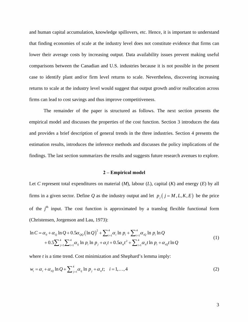
2 – Empirical model

Let C represent total expenditures on material (M), labour (L), capital (K) and energy (E) by all

firms in a given sector. Define Q as the industry output and let ( ), , ,jp j M L K E= be the price

of the jth input. The cost function is approximated by a translog flexible functional form

(Christensen, Jorgenson and Lau, 1973):

( ) 4 420 1 1

4 4 421 1 1

ln ln 0.5 ln ln ln ln

0.5 ln ln 0.5 ln ln

Q QQ i i iQ ii i

ij i j t tt it i tQj i i

C Q Q p p Q

p p t t t p t Q

α α α α α

α α α α α= =

= = =

= + + + +

+ + + + +

∑ ∑∑ ∑ ∑

(1)

where t is a time trend. Cost minimization and Shephard’s lemma imply:

4

1ln ln ; 1, , 4i i iQ ij j itj

w Q p t iα α α α=

= + + + =∑ … (2)

4

where iw is the ith input expenditure share. Homogeneity, adding-up and symmetry properties

imply that:

4 1iiα =∑ , 4 0iQi

α =∑ , 4

10iji

jα=

= ∀∑ , 4

10iti

α=

=∑ , and ij jiα α= (3)

Unfortunately, no parametric restrictions can simultaneously preserve the flexibility of the

translog cost function while guaranteeing that concavity in prices will be respected. The

concavity property of the translog cost function is data dependent. Ryan and Wales (2000)

showed how to impose concavity at a single point while preserving the global flexibility of the

cost function.1 While there is no assurance that their approach improves the overall number of

observations for which concavity is respected, they report that their method works extremely

well for their empirical application (i.e. concavity is automatically verified at all points).

Let H be the Hessian of the cost function defined in (1). Moreover, let *p , *Q and *t

represent the normalization points. In the empirical application that follows, they will represent

the province of interest for a specific year. It can be shown that the elements of the Hessian

evaluated at the normalization points are only function of the parameters of the model (Diewert

and Wales, 1987):

ij ij ij i i jH α δ α α α= − + ; , 1, , 4i j = … (4)

where 1ijδ = if i j= and 0 otherwise. The Hessian can be expressed as the product of a lower

triangular matrix D (with elements ijd ) by itself; i.e., '= −H DD which by definition is negative

semi-definite. Hence, (4) can be rewritten as:

( )ij ij i i jijα δ α α α′= − + −DD (5)

The parametric restrictions in (5) are imposed when estimating the cost function in (1)

and expenditures shares in (2). It is relatively straightforward to show that:

5

2 2 2 2 2 2 2 2 211 11 1 1 22 21 22 2 2 33 31 32 33 3 3

12 11 21 1 2 13 11 31 1 3 23 21 31 22 32 2 3

; ;

; ;

d d d d d d

d d d d d d d d

α α α α α α α α α

α α α α α α α α α

= − + − = − − + − = − − − + −

= − − = − − = − − − (6)

The parameters of the 4th input share equation are retrieved using the adding-up property.

Equations (1) and (2) are estimated by maximum likelihood once restrictions in (3) and (6) have

been included in the cost function and expenditure shares. The restricted system has the same

number of parameters as in (1) and thus Ryan and Wales’ methodology preserves the flexibility

of the translog cost function.

Canadian dairy production is under supply management and thus administered decisions

in the dairy industry will likely have impacts on the cost structure of processing firms. Assuming

that expenditures in material mainly include raw milk, material is not a choice variable from the

industry perspective and is a predetermined variable in the cost minimization process. It is

assumed that production of dairy products in a given province is determined according to the

Leontief-type technology: ( ) ( ){ }10, , , min , , ,M

MQ G M K L E M F K L Eαα= = . The production

process ( )G i implies that there are no substitution possibilities between material (milk) and the

other three production factors. It is assumed that the technology in the sub production function

( )F ⋅ can be approximated by a translog cost function. Hence the system of equations in the

dairy sector consists of equations (1) and (2) for , ,i L K E= as well as the following output

equation that summarizes the technological relationship between output of dairy products and

raw milk:

0 1ln ln lnM MQ Mα α= + (7)

The specification in (7) has the advantage that returns to scale are measured using

proportional variations in the production quota at the farm level. The current framework

explicitly accounts for proportional changes in the production quota when computing the impact

6

of a change in output on total costs. While predetermined quantities of milk could have been

modeled using a general translog cost function as in the bakery and meat sectors, a change in

processed dairy output would not have been accommodated through a proportional change in

material. The specification in (7) guarantees that this condition will be respected.

3 – Data

Data on input expenditures and sales receipts come from Statistics Canada’s Annual Survey of

Manufactures (ASM). The available data cover the period 1990-1999. Data were also available

for the 2000-2002 period, but important modifications were made to the coverage of the ASM in

2000. First, the survey stopped collecting data on hours worked in 2000 and this constitutes an

important limitation when computing a price index for labour. Second, the ASM started

including in 2000 all incorporated businesses with sales of less than $30,000 in manufactured

goods as well as all unincorporated manufacturers. Finally, major conceptual and methodological

changes were made to the ASM which resulted in total manufacturing shipments increasing by

about 8% between 1999 and 2000. The impacts of including the post-2000 data in the empirical

model are largely unknown and thus it was considered preferable to exclude these three years

from the sample. The data were collected by province and broken down across industry

according to the North American Industry Classification System (NAICS). The industries are the

bread and bakery sector (#3118), the meat sector (#3116) and the dairy sector (#3115).

Four inputs are used in the model: material, labour, energy and capital. While total

expenditures for the first three inputs are available in the ASM, capital expenditures must be

extracted from another dataset, Statistics Canada’s Cansim table 031-0002. The data is only

available at the national level and linear regressions were used to decompose aggregate capital

expenditures at the provincial level. The results of the different linear models that were used are

7

not reported here for sake of brevity. The estimation strategy consisted in specifying a

parsimonious linear equation in each sector. Capital expenditures were regressed on sales,

number of workers, material expenditures and energy costs, and any combination of these

variables. Each equation was used to produce predicted values of capital expenditures at the

provincial level. We selected the specification that minimized the distance between the

summation of the predicted capital expenditures in each province and the observed capital

expenditures at the national level. This criterion coincided with the model selection outcome

based on the Schwartz Bayesian Criterion. The national capital price index was applied to

expenditures in all provinces due to the lack of data to proxy provincial capital price indexes.

An output price index was needed to deflate total sales receipts in order to construct an

output measure. Unfortunately, the industrial price index in Cansim table 329-0038 is only

available starting in 1992 and is not available at the provincial level. Hence, it was decided to use

the consumer food price index in each province (Cansim table 326-0002). It is important to note

that each province uses a distinct reference price in computing the price index (1997 = 100) and

thus the index only accounts for variations in the time domain, and does not account for regional

differences in prices. Hence, the 1995 comparative price index for selected cities across Canada

was used to insert variability in the consumer food price index across provinces.

A price index for labour is computed from the ASM dataset using total wages paid to

production employees divided by hours of work. Price indexes for the other two inputs must be

obtained from sources other than the ASM. Because the material input mainly includes the farm

output sold to manufactures, the producer price index was used to deflate material expenditures.

While there is no clear-cut farm product that exactly fits the mix of raw material in each

processing sector, price indexes for grain, livestock and dairy products in Statistic Canada’s

8

Cansim database were used respectively for the bread and bakery, meat and dairy sectors.

Finally, the energy price index was proxied by the electricity price index in each province. Once

again, variations across provinces were computed; this time using differences in electricity prices

across major cities in Canada for the year 2001 as reported by Hydro-Quebec (2001).

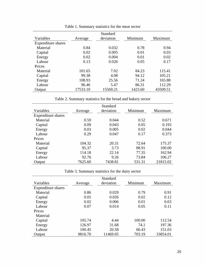
Tables 1, 2 and 3 present descriptive statistics of the meat, bread and bakery and dairy

sectors respectively. Note that the number of available observations differs across sectors.

Confidentiality issues will often result in a missing observation in the dataset. If the number of

firms is not sufficiently large, the observation at the industry level is withdrawn from the

database to prevent releasing information about individual firms. This leaves us with 44, 60 and

62 observations in the bread and bakery, meat and dairy sectors respectively. Material is included

in table 3 although the separability assumption for the dairy technology implies that the cost

share system only applies for energy, capital and labour. Still, it is interesting to compare the

factor intensity in the dairy industry with the other two industries. Tables 1, 2 and 3 report the

average expenditure share of each input with some information about their distribution. The

minimum and maximum values give an indication of the variability in shares across years and

provinces. In relative terms, the smallest variation in input expenditure shares occurs for material

which is also the most important expenditure share. This has important implications on scale

economies because as long as the price of material does not change with output, economies of

scale will be small because total costs are dominated by material expenditures. There are some

important variations in labour expenditures across observations. The greatest variation in the

price index in relative terms occurs for energy. It also seems that the bakery sector is the most

labour intensive of the three industries when measured in relative terms. Labour expenditures

represent a much smaller percentage of overall expenditures in the meat and dairy sectors.

9

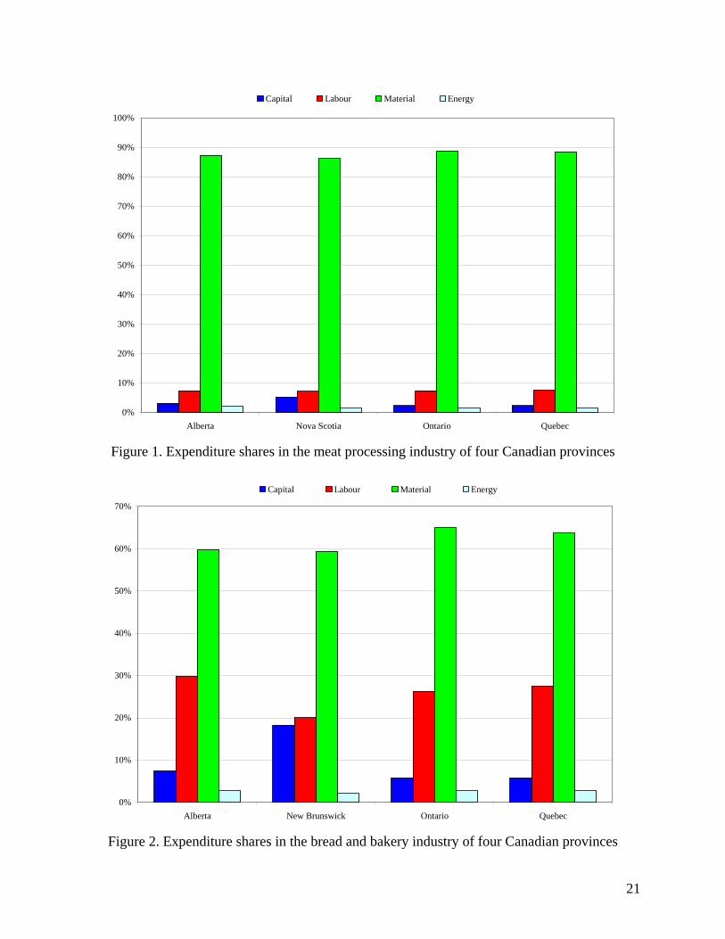
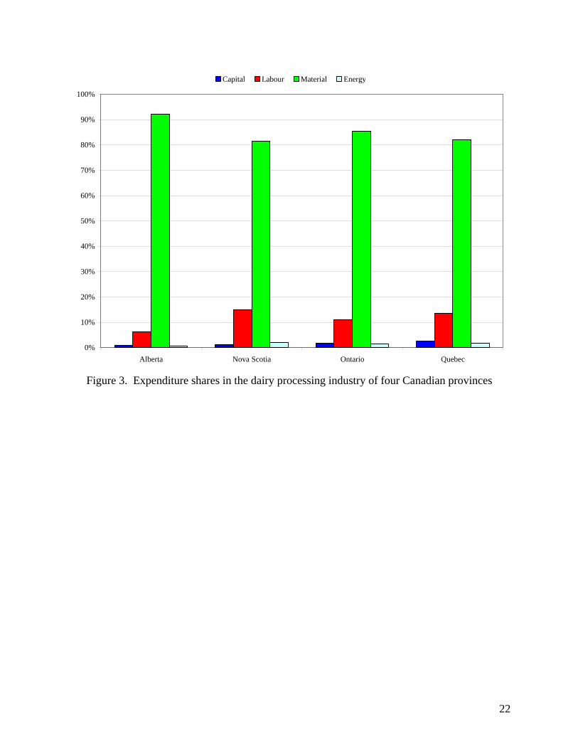
While tables 1, 2 and 3 provide an idea of the overall dispersion in the data, it is also

interesting to investigate whether there are important differences across provinces in a given

year. Figures 1, 2 and 3 present the input expenditure shares of four provinces in 1999 for the

meat, bread and bakery and dairy sectors respectively. Generally, speaking there is little variation

across provinces in 1999. However, the shares of capital and labour in the bread and bakery

sector of New Brunswick are significantly different than their Quebec, Ontario and Alberta

counterparts in Figure 2. Moreover, the difference between the material expenditure share

between Nova Scotia and Alberta is relatively important.

4 – Results

The model in (1)-(2) with the restrictions in (5) and (6) is highly non-linear and maximum

likelihood is used to estimate these equations. The statistics of interest are the scale elasticities in

each sector across large and small provinces. Preliminary runs revealed that imposing concavity

on the cost function did not yield the somewhat miraculous results of Ryan and Wales (2000) in

that concavity is not respected at all observations. One explanation is perhaps that there exists

greater heterogeneity across observations in the current sample than in Ryan and Wales’

empirical application. They used an annual time series of U.S. output manufacturing while the

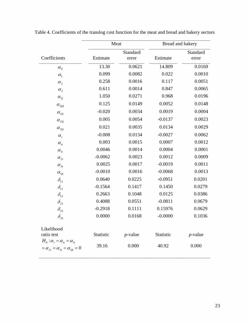
current sample includes small and large provinces. The estimated parameters of the meat and

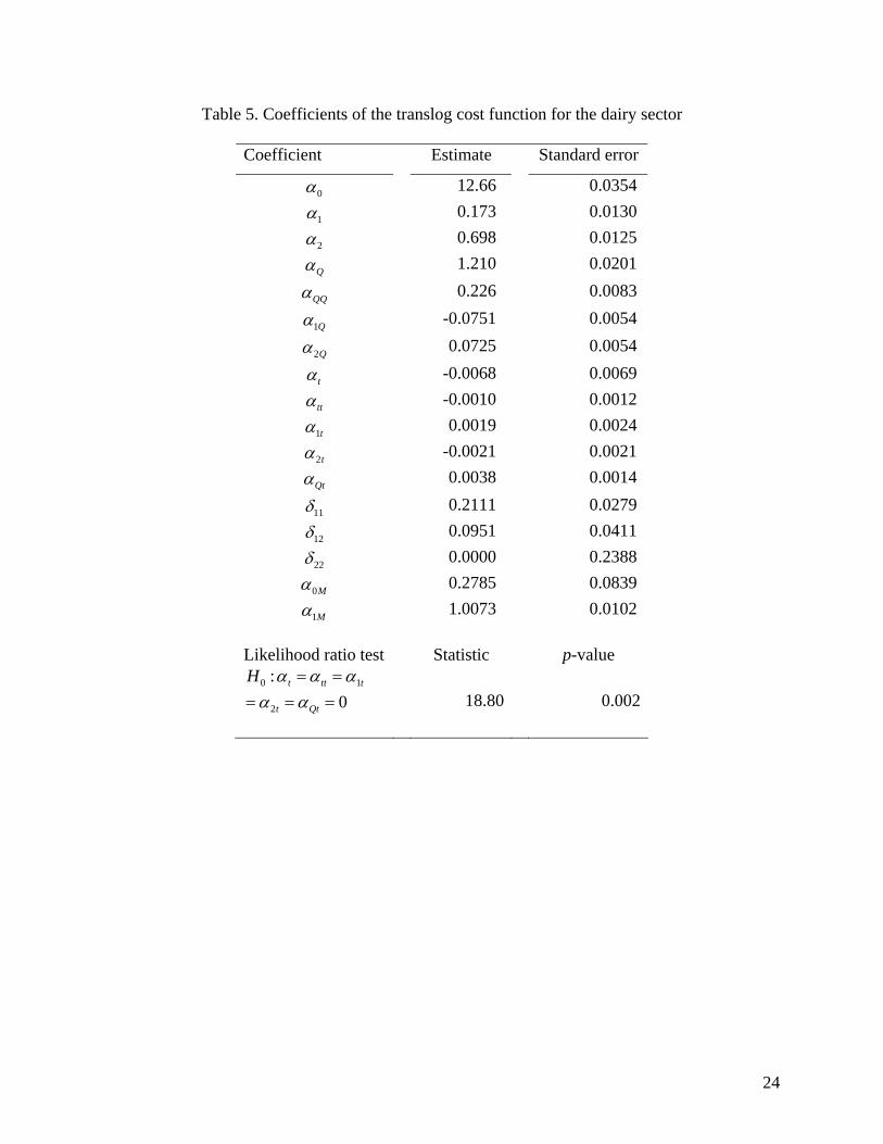
bread and bakery cost functions are reported in table 4 when concavity is imposed at the 1999-

Quebec observation. Table 5 presents the estimation results of the dairy cost function at the same

normalization point.

A Likelihood Ratio (LR) test was used to determine if a trend needed to be included in

the model. The LR statistic is: ( ) ( )2 ln lnU RLR L L= −⎡ ⎤⎣ ⎦ ; where UL and RL denote the value of

10

the likelihood function for the unrestricted and restricted ( )0;t tt it tQ iα α α α= = = = ∀ models

respectively. It follows a chi-squared distribution with 6 degrees of freedom. The LR statistic in

table 4 for the bread and bakery sector is 40.92 and yields a p-value less than 0.01 for the null

hypothesis that the trend coefficients are jointly not significant. Similar results hold for the meat

and dairy sectors. While the general fit of the empirical models seems adequate, it is difficult to

interpret the parameters as stand-alone meaningful economic statistics.2 For this purpose, the

notion of input substitutability and scale elasticities are introduced.

Blackorby and Russel (1989) argue that the notion of Hicksian substitutability among

inputs should be measured by the Morishima elasticities of substitution. The Morishima

elasticity (denoted by )ijM is computed as the derivative of the relative input use in logarithmic

form, ( )ln i jx x , with respect to the logarithmic of the price ratio i jp p . It is equal to

(Wohlgenant, 2001): ij ij jjM ε ε= − ; where ijε is the price elasticity of the demand for the ith

input with respect to the price of the jth input. The Morishima elasticities are data dependent; but

when evaluated at the normalization point, the uncompensated elasticities are strictly function of

the parameters: ( )ij ij ij i i j i jε α δ α α α α α= − + ; where 1ijδ = if i j= and zero otherwise.

The Morishima elasticities for the meat sector using the 1999-Quebec observation as the

normalization point are presented in table 6. While elasticities can differ across provinces and

time, unreported results suggest that they are rarely significantly different from a qualitative

standpoint. A particularly interesting elasticity is the change in the ratio of material to another

input following a change in the price of that other input. The substitution possibilities between

material and capital and material and energy do not seem to be negligible. For example, a one

percent decrease in the price of energy will decrease the ratio of materials to energy usage by

11

0.73 percent. Similarly, a decrease of 1% in the price of capital will decrease the ratio of material

to capital by 0.41 percent. Substitution seems to be more limited between material and labour.

Morishima elasticities in table 7 document substitution possibilities between all four

inputs for the bread and bakery sector. The results are strikingly different than substitution

elasticities for the meat sector. The ratio of material to labour is very price responsive with an

elasticity of 1. There is no substitution between material and capital as the point estimate of

elasticity is 0.01. As in the case of labour, the ratio of material to energy is quite elastic. The

most significant substitution effects involve energy as the Morishima elasticities are greater than

one. Morishima elasticities for the dairy sector are presented in table 8. By construction there are

no substitution possibilities between material and other inputs. As mentioned before, this rather

restrictive assumption was built in the model to account for the supply management policy. The

substitution elasticities between capital and energy are non negligible while there is less

substitution between labour and capital or energy.

Because all normalized data points equal one, it is relatively straightforward to compute

returns to scale evaluated at the normalization point given the logarithmic form of the cost

function. The scale elasticity in the meat and bread and bakery sectors are equal to the derivative

of the cost function with respect to output; and thus are directly measured by the parameter Qα .

A scale elasticity greater (lower) than one indicate decreasing (increasing) returns to scale.

Standard inference can be carried out in the usual way using asymptotic theory. Computing scale

elasticities in the dairy industry is however more involved because of the perfect

complementarity between material and the other inputs. The cost function is first divided up into

two sub cost-functions: one applies to expenditures in material while the second measures

expenditures in energy, capital and labour and has the translog form defined in (1). The sub-cost

12

function for material is: ( )1 1 11 0 1ln ln ln lnM M M M MC p Qα α α− − −= + + . Hence the scale elasticity

associated with expenditures in material is measured by 11Mα− while the scale elasticity of the

translog sub cost function is measured by Qα . Obviously, the total scale elasticity is not the sum

of the two separate elasticity measures. The following procedure is used to compute the total

scale elasticity: 1) compute fitted costs associated with each sub-cost function; 2) compute the

cost changes following a one percent change in output using the sub-cost scale elasticities ( Qα

and 11Mα− ); and 3) add up the predicted change in the two sub-costs and compare them to the

initial fitted costs in step 1.

Tables 9, 10 and 11 present the elasticities of scale of different provinces in 1999 for the

meat, bread and bakery and dairy sectors respectively. As mentioned before, concavity can only

be imposed locally if one wishes to preserve the flexibility of the cost function. To make sure

that the reported elasticity are consistent with the concavity property of the cost function being

verified, the model is re-estimated using each observation in the tables as a different

normalization point. While this procedure is lengthy, it has the advantage of being consistent

with the bootstrap procedure that is used below. Imposing concavity locally for the province of

Quebec in a given year may well result in concavity being verified for other provinces in many

different years; however, there is no guarantee that the non-violation of concavity will be

replicated in bootstrap samples. The only way to do so is to use a different normalization point

for the four reported cases when calculating the elasticities such that the bootstrap samples also

satisfy the concavity property.

Asymptotic confidence intervals are reported for the meat and bakery sectors. The

asymptotic distribution of the scale elasticity in the dairy sector is largely unknown because this

13

statistic involves many computations3 and thus bootstrap techniques were used. Moreover, it is

well known that the bootstrap distribution of a statistic provides a better estimate of the finite

sample distribution of the statistic than the asymptotic distribution if the statistic is

asymptotically pivotal (Horowitz, 2001).4 This may be especially true in the current context

given the relatively short samples. For the meat and bread and bakery sectors, the scale elasticity

parameters are not asymptotically pivotal because their distribution, although asymptotically

normal, depends on unknown population mean and variance parameters. The scale elasticity in

the dairy sector is also not pivotal because it is a combination of many parameters.

Beran (1987) has shown that the double bootstrap improves the accuracy of a single

bootstrap when an asymptotically pivotal statistic5 is not available by estimating a coverage error

for a confidence interval and then uses this estimate to adjust the single bootstrap thus reducing

its error. The double bootstrap method is relatively easy to implement and McCullough and

Vinod (1998) provide an excellent description of the algorithm that needs to be implemented. In

summary, let the initial maximum likelihood parameters be represented by the vector θ and the

predicted dependent variables by the matrix Y . Moreover, let the centered and rescaled sample

residuals be denoted by ε . Form a pseudo matrix of dependent variables *Y by sampling with

replacement from the matrix ε a matrix *ε such that ˆ* *Y = Y + ε . A bootstrap estimate of the

parameter of interest is obtained through maximum likelihood and is denoted *jθ . Repeat this

procedure J times.

For each bootstrap sample, the centered and rescaled residuals *ε are used to form a

second bootstrap sample ** * **= +Y Y ε . The model in (1)-(2) with restrictions in (5) and (6) is re-

estimated to obtain the vector of parameters **jkθ . This procedure is repeated K times. Compute

14

the pivotal statistic ( )** ˆ#j jkZ K= <θ θ . The idea is that under fairly general conditions, the

statistic jZ is uniformally distributed asymptotically (and thus is an asymptotically pivotal

statistic). Once all bootstrap samples are obtained, the statistics *jθ and jZ can be ordered

according to *(1)θ , *

(2)θ , …, *( )Jθ and (1)Z , (2)Z , …, ( )JZ . The simple bootstrap %α − confidence

interval is ( )( ) ( )* *

( 1)( 1) 1 , JJ ααθ θ ++ −⎡ ⎤⎣ ⎦ . The double bootstrap interval is ( ) ( )

* *( 1) ( 1),

L UJ Jα αθ θ+ +⎡ ⎤⎣ ⎦ where

( )( )( 1) 1L JZ αα + −= and ( )( 1)U JZ αα += . Hence, the role of the statistic Z is to redefine the

appropriate upper and lower bounds for the confidence intervals.

Table 9 suggests that there are increasing returns to scale in the meat sector because the

point estimate for all four provinces is below one. Hence, increasing industry output should

lower the industry’s average costs. Unfortunately, the asymptotic theory and bootstrap inference

do not rule out decreasing returns to scale as the upper bound of the 95% confidence interval is

greater than one. The single bootstrap interval does not seem different than the asymptotic

confidence interval. While the double bootstrap does not significantly change the conclusions of

the other two methods, it does provide some refinements to the confidence interval. It is

interesting to note that there is no statistically significant difference between the scale elasticities

in each province despite that production levels are quite different.

Table 10 presents the scale elasticities in the bread and bakery sector of Quebec, Alberta,

Ontario and New Brunswick. The asymptotic coverage for the scale elasticity parameter is

different than the coverage offered by the single percentile bootstrap method in the four

provinces. There exist significant returns to scale in the two smaller provinces (Alberta and New

Brunswick). The point estimate of the scale elasticity in Alberta suggests that a one percent

increase in output in 1999 would generate a 0.87 percent increase in total costs for the industry.

15

There exists decreasing returns to scale at the industry level for the sector in Ontario. While

increasing returns to scale in the Quebec industry cannot be ruled out from a statistical point, the

confidence interval is skewed to the right around the cut-off value of one; suggesting that the

industry cannot lower average costs by increasing output.

Table 11 provides the scale elasticity parameters for the dairy industry. The point

estimate for New Brunswick in 1999 is 0.93 which is statistically lower than one at the 95

percent confidence level both asymptotically and using the bootstrap inference. Hence, an

increase in output of 1% would only increase total costs in the industry by 0.93%. Note that this

increase in output must necessarily be accompanied by a proportional increase in material

according to the technology specification. In other words, dairy processors cannot increase

output without a corresponding increase in the production quota at the farm level. Hence, the

evidence suggests that the dairy processing industry in that province could move down its

average cost function by increasing output would milk production at the farm level be set

accordingly. The point estimate of the scale elasticity is however greater than one for the two

largest producing provinces, Quebec and Ontario. This suggests that increasing output at the

farm level would lead to increases in the industry average costs. It must be noted that these

conclusions hold in the context of 1999 and thus abstract from any potential structural change in

the industry (mergers, acquisitions, etc.) that has occurred since.

5 – Conclusion

Broad globalization forces in the agri-food sector are pressuring agri-food firms to increase their

competitiveness. In some instances, trade liberalization offers opportunities to expand output

while import competing agri-food industries may be forced in other instances to cut back

production. In any case, concentration and output expansion/contraction do affect the cost

16

structure of individual firms and the overall industry. The objective of the paper is to measure

potential (dis)economies of scale in the Canadian agri-food manufacturing sector. There has been

a considerable literature documenting economies of scale in U.S. agri-food industries but no

attention has been devoted to Canadian industries. U.S. and Canadian firms compete in common

markets and most likely share many similarities from a technological perspective. However, the

existence of supply management at the Canadian farm level and potential differences in factor

prices can lead to substantial differences in the overall cost structure of Canadian and U.S. food

processing firms.

Cost functions for three Canadian manufacturing agri-food sectors (meat, bakery and

dairy) are estimated using provincial data from 1990 to 1999. The Christensen, Jorgensen and

Lau (1973) translog flexible functional form is used. The concavity property of the cost function

is imposed locally using the approach of Ryan and Wales (2000). The Morishima substitution

elasticities in the bakery sector indicate that substitution possibilities between material and

energy and material and labour are important. Conversely, substitution possibilities between the

farm input and the other inputs in the meat sector are less significant. To account for the

implications of supply management on the cost structure of dairy processing firms, strong

separability between material and the other inputs was introduced through a Leontief technology

which yields two sub-cost functions that are estimated jointly. The sub-cost function for

expenditures in milk is log-linear while the sub-cost function for expenditures on capital, labour

and energy has the translog form. This rather stringent assumption on the technology was

introduced to account for the exogenous supply of milk at the farm level and more importantly to

restrict changes in processed dairy products to be accompanied by proportional changes in the

supply of raw milk at the farm level.

17

Inference is carried out using the usual asymptotic theory as well as bootstrap inference.

In particular, the ability of the double bootstrap to provide refinements in inference is

investigated. The idea of the double bootstrap is to sample from the initial bootstrap sample in

order to form an asymptotically pivotal statistic. This statistic is used to correct the inference

generated by the initial bootstrap sample. Scale elasticity parameters indicate that increasing

returns to scale are present in small bakery industries. Point estimates suggest that increasing

returns to scale exist at the industry level in the meat sector, but statistical inference cannot rule

the existence of decreasing returns to scale. Moreover, there are no statistical differences in the

measure of returns to scale across provinces. Finally, there exists evidence of increasing returns

to scale at the industry level in the dairy industries of Alberta and New Brunswick. The scale

elasticity for the two largest provinces (Ontario and Quebec) is greater than one, but inference

does not reject the null hypothesis of increasing returns to scale. The bootstrap method is

particularly helpful to compute confidence intervals in the dairy sector because the asymptotic

theory is practically difficult to compute in that case.

The major limitation of the study is the impossibility to distinguish the source of returns

to scale in the dataset. The provincial data yields elasticities of scale at the industry level that

encompass plant-level and firm-level economies of scale as well as economies of scale external

to firms. Future research endeavours should focus on breaking the data limitation barriers and

investigate with firm level data the cost structure of Canadian food processors. In that case,

meaningful comparisons could be drawn with the U.S. industry.

18

References Arrow, K. J., “Innovations and Increasing Returns to Scale”, in Increasing Returns and

Economic Analysis, edited by K. J. Arrow, Y-K Ng, and X. Yang, New York: St. Martin's Press, 1998.

Baldwin, J., D. Sabourin and D. West, Advanced Technology in the Canadian Food Processing

Industry, Agriculture and Agri-food Canada and Statistics Canada, 1999, Ottawa. Ball, V.E., and R.G. Chambers. “An Economic Analysis of Technology in the Meat Products

Industry”, American Journal of Agricultural Economics 64(1982): 699–709. Beran, R. “Prepivoting to Reduce Level Error in Confidence Sets”, Biometrika, 74(1987): 457-468. Blackorby, C. and R. R. Russell, “Will the Real Elasticity of Substitution Please Stand Up? A

Comparison of the Allen/Uzawa and Morishima Elasticities”, American Economic Review 79 (1989): 882-888.

Christensen, L. R., D. W. Jorgenson and L. J. Lau, “Transcendental Logarithmic Production

Frontiers”, Review of Economics and Statistics 55(1973): 28-45. Diewert, W. E., “An Application of the Shephard Duality Theorem: A Generalized Leontief

Production Function," Journal of Political Economy 79(1971): 481-507. Diewert, W. E. and T. J. Wales, “Flexible Functional Forms and Global Curvature Conditions”,

Econometrica 55(1987): 43-68. Greene, W. H., Econometric Analysis, 5th Edition, Prentice Hall, NJ, 2003. Horowitz, J., “The Bootstrap”, in Handbook of Econometrics Vol. 5, edited by J. J. Heckman and

E. Leamer, Elsevier Science, North Holland, 2001. Hydro-Quebec, Comparison of Electricity Prices in Major North American Cities, 2001. Kumbhakar, S. C., “Allocative Distortions, Technical Progress, and Input Demand in U.S. Airlines: 1970-1984”, International Economic Review 33(1992): 723-737. Lopez, R. A., A. M. Azzam, and C. Liron-Espana, “Market Power and/or Efficiency: A

Structural Approach”, Review of Industrial Organization 20(2002): 115-26. Macdonald, J. M., and M. E. Ollinger, “Scale Economies and Consolidation in Hog Slaughter”,

American Journal of Agricultural Economics (2000): 334-346. McCullough, B. D., and H. D. Vinod, “Implementing the Double Bootstrap”, Computational

Economics 12(1998): 79-95.

19

Morrison Paul, C. J., “Cost Economies and Market Power: The Case of the U.S. Meat Packing

Industry”, Review of Economics and Statistics 83 (2001a): 531-540. Morrison Paul, C. J., “Market and Cost Structure in the U.S. Beef Packing Industry: A Plant-

Level Analysis”, American Journal of Agricultural and Economics 83(2001b): 64-76. Ollinger, M., J. M. MacDonald, and J. M. Davidson, “Technological Change and Economies of

Scale in U.S. Poultry Processing”, American Journal of Agricultural Economics 87(2005): 87: 116-129.

Ryan, D. L., and T. J. Wales, “Imposing Local Concavity in the Translog and Generalized

Leontief Cost Functions”, Economics Letters 67(2000): 253-260. Wohlgenant, M. K., “Scale Economies and Consolidation in Hog Slaughter: Comment”,

American Journal of Agricultural Economics 83(2001): 1082-1083.

20

Table 1. Summary statistics for the meat sector

Variables

Average

Standard deviation

Minimum

Maximum

Expenditure shares Material 0.84 0.032 0.78 0.94 Capital 0.02 0.005 0.01 0.03 Energy 0.02 0.004 0.01 0.02 Labour 0.13 0.026 0.05 0.17Prices Material 101.65 7.02 84.23 115.41 Capital 99.38 4.08 94.12 105.21 Energy 108.93 25.56 71.24 165.88 Labour 96.46 5.47 86.31 112.29Output 17533.10 15569.21 1423.60 43509.51

Table 2. Summary statistics for the bread and bakery sector

Variables

Average

Standard deviation

Minimum

Maximum

Expenditure shares Material 0.59 0.044 0.52 0.671 Capital 0.09 0.043 0.05 0.193 Energy 0.03 0.005 0.02 0.044 Labour 0.29 0.047 0.17 0.373Prices Material 104.32 20.31 72.64 175.37 Capital 95.37 3.73 88.91 100.00 Energy 114.18 22.14 77.35 162.94 Labour 92.76 9.26 73.84 106.27Output 7625.60 7438.81 531.31 21815.02

Table 3. Summary statistics for the dairy sector

Variables

Average

Standard deviation

Minimum

Maximum

Expenditure shares Material 0.86 0.029 0.79 0.91 Capital 0.05 0.026 0.02 0.12 Energy 0.02 0.006 0.01 0.03 Labour 0.07 0.014 0.05 0.11Prices Material Capital 105.74 4.44 100.00 112.54 Energy 126.97 31.68 74.1 197.36 Labour 100.45 20.58 66.43 151.03Output 9816.70 11469.05 703.19 33854.01

21

0%

10%

20%

30%

40%

50%

60%

70%

80%

90%

100%

Alberta Nova Scotia Ontario Quebec

Capital Labour Material Energy

Figure 1. Expenditure shares in the meat processing industry of four Canadian provinces

0%

10%

20%

30%

40%

50%

60%

70%

Alberta New Brunswick Ontario Quebec

Capital Labour Material Energy

Figure 2. Expenditure shares in the bread and bakery industry of four Canadian provinces

22

0%

10%

20%

30%

40%

50%

60%

70%

80%

90%

100%

Alberta Nova Scotia Ontario Quebec

Capital Labour Material Energy

Figure 3. Expenditure shares in the dairy processing industry of four Canadian provinces

23

Table 4. Coefficients of the translog cost function for the meat and bread and bakery sectors

Meat Bread and bakery

Coefficients

Estimate

Standard error

Estimate

Standard error

0α 13.30 0.0621 14.809 0.0169

1α 0.099 0.0082 0.022 0.0010

2α 0.258 0.0016 0.117 0.0051

3α 0.611 0.0014 0.847 0.0065

Qα 1.050 0.0271 0.968 0.0196

QQα 0.125 0.0149 0.0052 0.0148

1Qα -0.020 0.0034 0.0019 0.0004

2Qα 0.005 0.0054 -0.0137 0.0023

3Qα 0.021 0.0035 0.0134 0.0029

tα -0.008 0.0134 -0.0027 0.0062

ttα 0.003 0.0015 0.0007 0.0012

1tα 0.0046 0.0014 0.0004 0.0001

2tα -0.0062 0.0023 0.0012 0.0009

3tα 0.0025 0.0017 -0.0019 0.0011

Qtα -0.0010 0.0016 -0.0068 0.0013

11δ 0.0640 0.0225 -0.0951 0.0201

12δ -0.1564 0.1417 0.1450 0.0279

13δ 0.2663 0.1048 0.0125 0.0386

22δ 0.4088 0.0551 -0.0811 0.0679

23δ -0.2918 0.1111 0.15976 0.0629

33δ 0.0000 0.0168 -0.0000 0.1036 Likelihood ratio test

Statistic

p-value

Statistic

p-value

0 1: t tt tH α α α= =

2 3 0t t Qtα α α= = = = 39.16 0.000 40.92 0.000

24

Table 5. Coefficients of the translog cost function for the dairy sector

Coefficient Estimate Standard error

0α 12.66 0.0354

1α 0.173 0.0130

2α 0.698 0.0125

Qα 1.210 0.0201

QQα 0.226 0.0083

1Qα -0.0751 0.0054

2Qα 0.0725 0.0054

tα -0.0068 0.0069

ttα -0.0010 0.0012

1tα 0.0019 0.0024

2tα -0.0021 0.0021

Qtα 0.0038 0.0014

11δ 0.2111 0.0279

12δ 0.0951 0.0411

22δ 0.0000 0.2388

0Mα 0.2785 0.0839

1Mα 1.0073 0.0102 Likelihood ratio test Statistic p-value

0 1: t tt tH α α α= =

2 0t Qtα α= = = 18.80 0.002

25

Table 6. Morishima input price elasticities in the meat sector

Price change Quantity ratio

(numerator) Capital Labour Material Energy

Capital 0.86 0.08 0.44

Labour 0.53 0.13 0.73

Material 0.41 0.25 0.73

Energy 0.07 0.42 0.97

Table 7. Morishima input price elasticities in the bread and bakery sector

Price change Quantity ratio

(numerator) Capital Labour Material Energy

Capital 0.84 0.08 1.48

Labour 0.08 0.88 1.44

Material 0.01 1.01 1.38

Energy 0.39 1.38 0.63

Table 8. Morishima input price elasticities in the dairy sector

Price change Quantity ratio

(numerator) Capital Labour Energy

Capital -0.101 1.107

Labour 0.237 0.769

Energy 0.775 0.230

26

Table 9. Scale elasticities in the meat sector Asymptotic Single bootstrap Double bootstrap

Province

Elasticity point

estimate Lower Upper Lower Upper Lower Upper

Quebec 0.97 0.93 1.01 0.93 1.01 0.94 1.00

Ontario 0.97 0.92 1.02 0.92 1.01 0.92 1.01

Alberta 0.97 0.93 1.02 0.93 1.02 0.92 1.01

Nova Scotia 0.96 0.91 1.01 0.91 1.01 0.91 1.00

Table 10. Scale elasticities in the bread and bakery sector

Asymptotic Single bootstrap Double bootstrap

Province

Elasticity point

estimate Lower Upper Lower Upper Lower Upper

Quebec 1.05 1.00 1.11 0.97 1.11 0.99 1.11

Ontario 1.12 1.06 1.18 1.03 1.19 1.06 1.19

Alberta 0.87 0.82 0.92 0.80 0.94 0.81 0.92

New Brunswick 0.78 0.72 0.83 0.71 0.85 0.72 0.83

Table 11. Scale elasticities in the dairy sector

Single bootstrap Double bootstrap

Province

Elasticity point

estimate Lower Upper Lower Upper

Quebec 1.01 0.99 1.04 0.97 1.05

Ontario 1.01 0.98 1.03 0.97 1.06

Alberta 0.97 0.94 0.99 0.93 1.01

New Brunswick 0.93 0.91 0.96 0.89 0.96

27

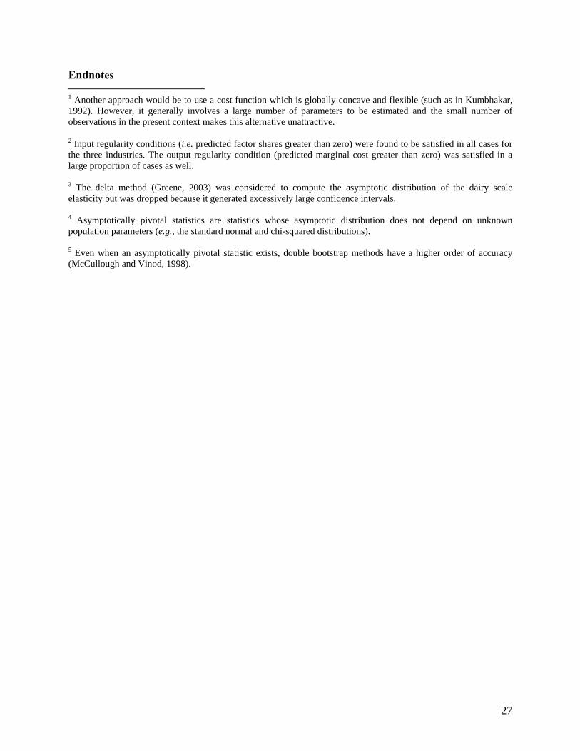
Endnotes 1 Another approach would be to use a cost function which is globally concave and flexible (such as in Kumbhakar, 1992). However, it generally involves a large number of parameters to be estimated and the small number of observations in the present context makes this alternative unattractive. 2 Input regularity conditions (i.e. predicted factor shares greater than zero) were found to be satisfied in all cases for the three industries. The output regularity condition (predicted marginal cost greater than zero) was satisfied in a large proportion of cases as well. 3 The delta method (Greene, 2003) was considered to compute the asymptotic distribution of the dairy scale elasticity but was dropped because it generated excessively large confidence intervals. 4 Asymptotically pivotal statistics are statistics whose asymptotic distribution does not depend on unknown population parameters (e.g., the standard normal and chi-squared distributions). 5 Even when an asymptotically pivotal statistic exists, double bootstrap methods have a higher order of accuracy (McCullough and Vinod, 1998).