ECONOMICS

REGIONAL EQUALITY AND NATIONAL DEVELOPMENT IN CHINA: IS THERE A

TRADE-OFF?

by

Anping Chen School of Economics

Jinan University

and

Nicolaas Groenewold Business School

The University of Western Australia

DISCUSSION PAPER 09.21

1

Regional Equality and National Development in China: Is There a Trade-Off?

Anping Chen,

School of Economics,

Jinan University,

Guangzhou, 510632,

Guangdong Province,

China

e-mail: anping.chen@yahoo.com.cn

and

Nicolaas Groenewold,*

Department of Economics,

University of Western Australia,

Crawley, WA 6009

Australia

e-mail: nic.groenewold@uwa.edu.au

*Corresponding author.

We are grateful to the Australian Department of Education, Employment and Workplace

Relations and to the Business School at UWA for support for Chen to visit UWA under

the Endeavour Award scheme in 2009 and to the Department of International Co-

operation at Jinan University and the UWA Business School for grants which supported

the visit of Groenewold to Jinan University in 2008. We have benefited from comments

received from participants in the Economics Seminar at the University of Western

Australia, from members of the China Economy and Business Program at the Australian

National University and from members of a seminar at the China Center for Economic

Studies at Fudan University.

2

Regional Equality and National Development in China: Is there a Trade-Off?

Abstract:

Despite high economic growth over the past 30 years, China’s substantial and persistent

regional disparities have been the subject of continuing concern to policy makers, as well

as the target of a wide variety of policies. An important issue in the policy debate about

whether and how best to attack these disparities is whether measures designed to improve

regional equality come at a cost to national development, i.e. whether there is a trade-off

between the level of national output and the equality of its distribution across the regions.

There is little analysis of this issue in the literature. We help fill this gap by setting up a

two-region model designed to capture some of the salient features of the Chinese

economy. We subject this model to a number of policy shocks and assess the effects on

regional disparities in per capita output, on the one hand, and on aggregate output on the

other to investigate the trade-off. We also consider income and welfare as alternatives to

output. We find that disparities in per capita output, income and welfare often move in

different directions so that it is important to specify which disparity is being targeted.

Moreover, since both disparities and aggregate outcomes are endogenous, how they move

together depends on the nature of the shock driving the model. Thus, some policies

designed to reduce disparities face a trade-off and others do not. Only a reduction in

internal migration restrictions unambiguously reduces all three disparity measures and

increases aggregate output, income and welfare. All other policies considered face a

trade-off in at least one dimension.

(265 words)

Key words: regional disparities, China, national output, trade-off, numerical modelling

JEL classifications: O18, O23, R11, R12, R13

3

1. Introduction

That aggregate growth in China has been high for several decades is well known.

Even the recent “Global Financial Crisis” has had relatively little impact, with China

being a central engine for world economic growth in the face of faltering economies

around the globe. What is perhaps somewhat less well known is that the regional

distribution of Chinese prosperity has been very uneven and is likely to continue to be so

for the foreseeable future. This dark underside of the Chinese “economic miracle” has

not gone unnoticed by Chinese policy makers at the highest level and central government

policy to address this issue has been a continuing feature of macroeconomic policy.1

Policy to reduce regional disparities are clearly desirable on the basis of equity

and have also been supported on the basis of the danger of social unrest which might be

caused by widening gaps between rich and poor regions. Yet, there has been a noticeable

caution in the vigour with which such policies are pursued by policy makers who are

reluctant to jeopardise the continuation of a high aggregate growth rate. Thus, there is, in

some quarters at least, a perception that directing policy to improve regional equality may

have a cost in terms of lower national performance; that is, there is the perception of a

trade-off between national output and the equality of its distribution across the regions.

If there is such a trade-off, it is clearly an important constraint on the execution of

policy. Yet there has been little analysis of this issue either at a theoretical or empirical

level. This is not surprising since the resolution of the question is not likely to be simple;

after all, in any reasonable macroeconomic model inter-regional per capita output

disparities and aggregate output will both be endogenous so that whether they move

1 See Groenewold et al. (2008), Chapter 2 and 3 for detailed information on Chinese regional disparities

and regional policy since the founding of the People’s Republic of China.

4

together or not will, in general, depend on the nature of the shock driving the model. In

policy terms, we would expect the existence of a trade-off to depend on the policy being

used to pursue equality. If this is indeed the case, it is all the more important to

investigate this issue since some policies may be constrained by a serious trade-off while

others may not.

Of course, those familiar with the literature on economic development and on

regional development in particular, will realise that the consideration of such a trade-off

is not new. Indeed, it dates back at least to the work on the inverted-U curve between

economic development and regional inequality; see particularly Williamson (1965) and

earlier work by Kuznets (1955) and Myrdal (1957) and Hirschman (1958). The idea

captured by the inverted-U curve is that in the early stages of development regional (and

other) inequality rises but eventually falls as development (usually measured in terms of

income or output per capita) proceeds. There is thus a relationship between inequality

and development which has an inverted-U shape. A recent discussion by Golley (2007,

Chapter 2) develops the relationship between these papers and explores possible

underlying mechanisms.

While the original literature focused on the relationship between (per capita)

output or income and disparities, many of the empirical applications came from growing

economies. Moreover, policy applications were also often to growing economies so that

in more recent literature the question is often cast in terms of the relationship between

growth and inequality.2 A substantial theoretical and empirical literature has developed

in this area but little consensus has been reached. Thus theoretical analysis in papers by

2 But see Chang and Ram (2000) and Easterly (2007) for recent examples of analyses of the relationship

between per capita income and inequality.

5

Galor and Zeira (1993), Alesina and Rodrik (1994), Persson and Tabellini (1994) and

Benhabib and Rustichini (1996) present arguments that growth and inequality are

negatively related while Kaldor(1956), Benabou (1996), Edin and Topel (1997) argue the

opposite effects. Empirical work is equally inconclusive with the work reported in papers

by Alesina and Rodrik (1994) and Persson and Tabellini (1994) finding that inequality is

harmful for growth while Forbes (2000) reports the opposite finding and various papers

present ambiguous results including those by Barro (2000), Partridge (2005), Fallah and

Partridge(2007), Chambers (2007), Bjornskow (2008) and Barro (2008).

The literature on inequality and development in China is relatively sparse. Li and

He (2006) recently predicted that China will continue to maintain rapid economic growth

during the 11th

Five-Year plan but that the income gap between regions will be further

enlarged because of three factors: continuing structural adjustment, the deepening of

administrative reforms and the enhancing of market forces. Kuijs and Wang (2005)

argue that China can have a more balanced growth path with a sustainable reduction of

income inequality if appropriate policies, such as reducing subsidies to industry and

investment, encouraging the development of the services industry and reducing the

barriers to labour mobility are implemented. Wan et al. (2006) explicitly tested the

growth-inequality nexus in China, focusing on rural-urban income inequality and regional

growth using a provincial-level panel data set. They found that an increase of inequality

has negative effects on growth irrespective of time horizons. Finally, Qiao et al. (2008)

find that fiscal decentralisation has resulted in more rapid economic growth accompanied

by greater regional inequality.

6

To sum up, there is a substantial literature, both theoretical and empirical, in the

broadly-defined area of inequality and development but no consensus on the direction of

the relationship between them. Moreover, there is relatively little work which deals

explicitly with China.

Our paper contributes to filling this gap. Our contribution to the literature is four-

fold. First, we revert to the original question of the relationship between inequality and

(per capita) output in contrast to much of the literature which has focused on the growth

of output. Second, we extend the analysis from one of output to include income and

welfare. We are thus able to look at inter-regional inequality and national development in

terms of three alternative measures: output, income and welfare. Third, we focus on

inter-regional disparities rather than household income or urban-rural inequality. This

reflects, in part at least, an important policy focus in China. Fourth, we recognise the

joint endogeneity of the two variables: the inter-regional gap and the national level of

output (or income or welfare). This approach is in contrast to much of the empirical

literature which tends to consider causation from inequality to growth or output and

ignores the possibility of reverse causation. Our analysis follows arguments by Lundberg

and Squire (2003) that a two-way relationship between these variables ought to be

entertained.

Our approach is theoretical and we proceed by setting up a simple theoretical

economic model which we subject to a variety of shocks designed to simulate policy

actions. We then observe the effects on both inter-regional disparities and national

variables to assess the trade-off question.

7

To keep the analysis tractable, we distinguish only two regions (based on the

widely-used interior/coastal distinction in China), we allow inter-regional migration but

with a cost to reflect the Chinese household registration or hukou system and we capture,

in a rudimentary way, some of the features of the Chinese taxation and expenditure

system. Naturally, we abstract from many other features of the economy.

Notwithstanding the simplicity of the model, it is non-linear and relatively

intractable so that, before using it to address the trade-off question, we linearise it in

terms of proportional changes and go on to solve it in numerical form, calibrating the

linearised model using recent data for China. Our model can, therefore, be seen as a

(very) small computable general-equilibrium (CGE) model, but one which, in contrast to

commonly-used CGE models, is relatively transparent.

While the model is designed to capture some features of the Chinese economy and

is calibrated with Chinese data, we argue that with some exceptions (such as a relaxation

of the internal migration restrictions) many of the policies simulated are more widely

applicable than just to China.

The structure of our model is most closely related to three recent theoretical

papers on China which use numerical models, one by Hu (2002), one by Hertel and Zhai

(2006) and a third by Whalley and Zhang (2007). While all these papers use small

numerical models of (aspects of) the Chinese economy, none of them focuses on policy

measures which might be used to reduce regional disparities and, moreover, none

addresses the trade-off question.

The general nature of our findings can be briefly summarised as follows. First,

different gaps (i.e. in per capita output , income or welfare) do not generally all move in

8

the same direction so that policy needs to be clear as to which gap is being targeted.

Second, whether a narrowing of the gap between the interior and the coast comes at the

expense of the national level of the relevant variable depends on the policy shock which

drives the change. Third, whether there is a trade-off or not depends on the variable of

interest. Fourth, most policies face a trade-off in at least one of the three dimensions

examined.

2. The model

To keep the regional structure of the model as simple as possible, we assume that

there are two regions conventionally called the coastal and interior (or inland) regions.

This two-region scheme has been widely used in policy discussion until the mid-1980s

and continues to be widely used in empirical work on China.3 The two-region

disaggregation we use is illustrated in Figure 1.

[Figure 1 about here]

The coastal region is relatively wealthy compared to the interior. Moreover,

agriculture which has been central to the Chinese economy is still a major source of

income and employment in the inland provinces while its importance has been supplanted

by manufacturing in the coast. We capture these stylised facts starkly by assuming a poor

interior region (denoted by I) which produces agricultural goods (denoted by A) and a

wealthy coastal region (denoted by C) which produces manufactured goods (denoted by

M).

3 Recent papers using this classification are Fleisher and Chen (1997), Demurger(2001), Fujita and Hu

(2001), Bao et al., (2002), Brun et al. (2002), Hu (2002), Whalley and Zhang (2007) and He, Wei and Xie

(2007).

9

Each region has households, firms and regional governments. There is also a

central government. Households supply labour to firms which produce output.

Households receive wage and profit income which they use to purchase some of each

region’s output; in addition, they receive a government-provided consumption good

which is private in the rival sense. Firms produce output using three factors – labour, a

fixed factor (land or capital) and a government-provided public good (which we call

infrastructure). No factors are inter-regionally mobile in the short run but labour can

migrate between regions in the long run although there are migration restrictions. In

principle, it would be straightforward to introduce capital mobility but this would make

the interpretation of the results more complicated and distract from our focus on labour

migration, governments and relative price changes as connections between regions.

Besides, there is recent evidence (Li, 2009) that capital mobility between China’s

provinces is much lower than is consistent with free capital mobility.

We distinguish between central and regional governments, with the latter

including all sub-national government levels although we recognise that, in practice, the

latter level includes several layers (provincial, prefecture, county and township). This

distinction between two levels of government is an important part of our model since

both regional and central governments can be expected to implement policies which have

regional objectives and effects.

In our model, both levels of government provide households with a consumption

good. From the households’ perspective the government-provided consumption good is

homogeneous. In addition to the consumption good, the regional governments are

assumed to provide infrastructure which is an input into the production process.

10

On the taxation side, we assume three taxes in the model in a way which broadly

reflects the stylised facts of the Chinese taxation system: (i) a national value-added tax

(VAT), the rate for which is set by the central government at the same level for both

regions and the proceeds from which are shared between the central government and the

regions with the same shares for each region;4 (ii) a business tax levied by the coastal

government which is assumed to be levied on the value of manufacturing output; (iii) an

agricultural tax which we assume to be levied on the value of agricultural output by the

interior government.5

We assume that households supply labour inelastically to firms in their own

region (each household supplying one unit) and choose consumption to maximise utility.

In the coastal region, manufacturing firms choose employment and output to maximise

profits, taking the real wage as a parameter and, in the interior, agricultural firms employ

all labour and pay a wage equal to the average product of labour. Governments are

assumed to behave exogenously apart from the fact that they need to satisfy their budget

constraint.

We consider the behaviour of households, firms and governments in turn.6

4 Although in the simulations we allow these shares to differ so that we can use them to model a fiscal

transfer. 5 While our structure drastically simplifies the structure of Chinese taxes, we would argue that it captures

the salient features; see Zhang and Martinez-Vazquez (2003), Jin, Qian and Weingast (2005), Shen, Jin and

Zou (2006), Jin and Zou (2005), Tochkov (2007), Zhang and Zou (1998), Zhang and Zou (2001) and

Zhang (2006) for recent information on aspects of the Chinese public finances. It should be also noted that

the tax on agriculture was abolished in 2006. We nevertheless include it in our model since for much of the

postwar period it has been an important source of revenue for the interior provincial governments. But it

would be possible to replace it with an alternative that falls more heavily on the interior provinces and is an

important source of revenue for them. Indeed and ironically, our analysis will be useful to assess the likely

effectiveness of the abolition of this tax in reducing the gap between the inland and the coast. 6 A list of variables is given in Appendix 1.

11

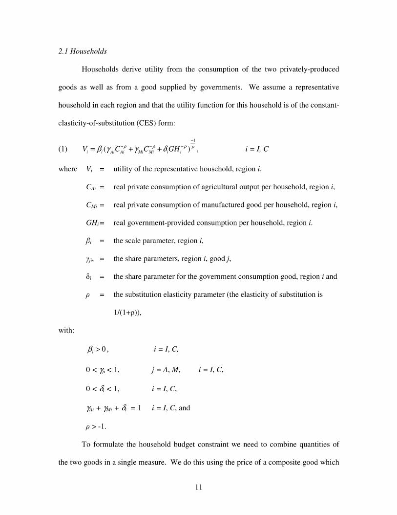
2.1 Households

Households derive utility from the consumption of the two privately-produced

goods as well as from a good supplied by governments. We assume a representative

household in each region and that the utility function for this household is of the constant-

elasticity-of-substitution (CES) form:

(1)

1

( )i i Ai Ai Mi Mi i i

V C C GHρ ρ ρ ρβ γ γ δ

−

− − −= + + , i = I, C

where Vi = utility of the representative household, region i,

CAi = real private consumption of agricultural output per household, region i,

CMi = real private consumption of manufactured good per household, region i,

GHi = real government-provided consumption per household, region i.

βi = the scale parameter, region i,

γji, = the share parameters, region i, good j,

δi = the share parameter for the government consumption good, region i and

ρ = the substitution elasticity parameter (the elasticity of substitution is

1/(1+ρ)),

with:

0i

β > , i = I, C,

0 < γji < 1, j = A, M, i = I, C,

0 < δi < 1, i = I, C,

γAi + γMi + δi = 1 i = I, C, and

ρ > -1.

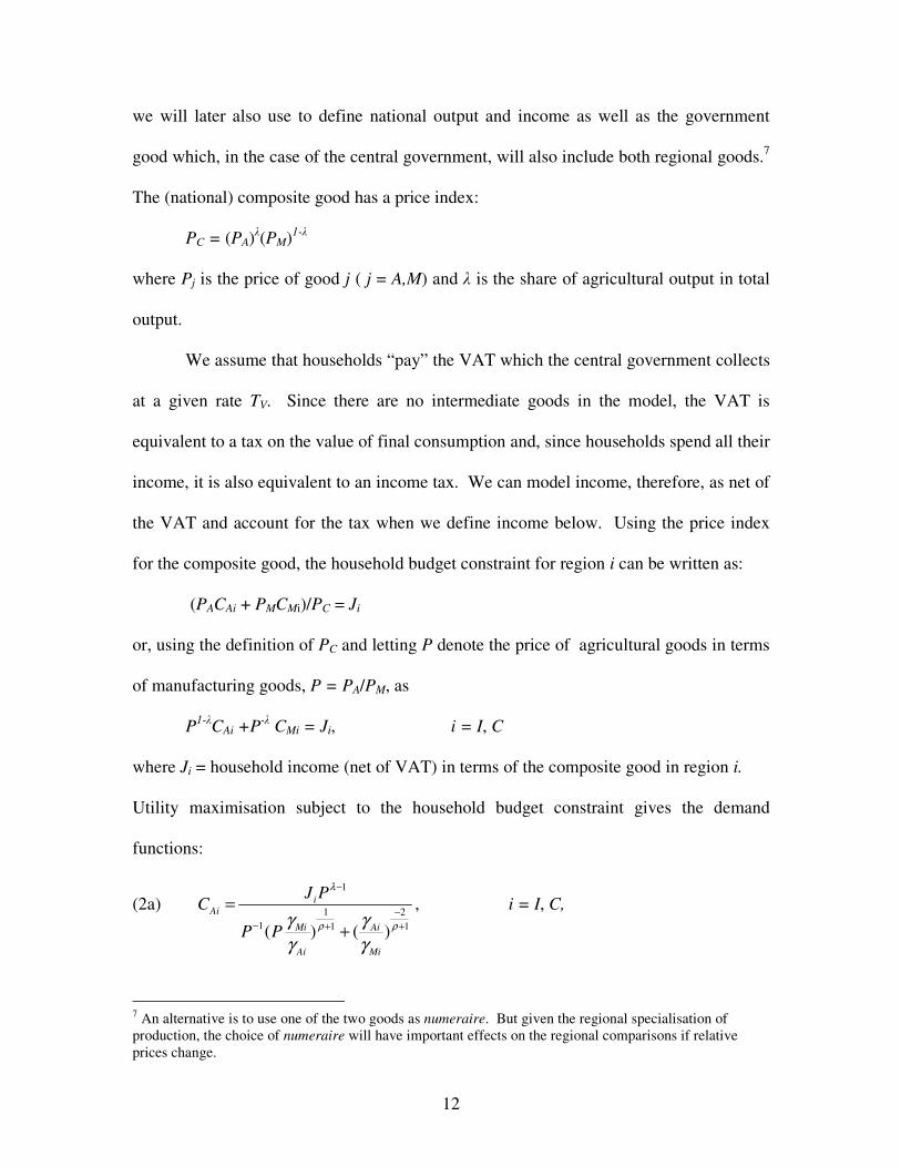
To formulate the household budget constraint we need to combine quantities of

the two goods in a single measure. We do this using the price of a composite good which

12

we will later also use to define national output and income as well as the government

good which, in the case of the central government, will also include both regional goods.7

The (national) composite good has a price index:

PC = (PA)λ(PM)

1-λ

where Pj is the price of good j ( j = A,M) and λ is the share of agricultural output in total

output.

We assume that households “pay” the VAT which the central government collects

at a given rate TV. Since there are no intermediate goods in the model, the VAT is

equivalent to a tax on the value of final consumption and, since households spend all their

income, it is also equivalent to an income tax. We can model income, therefore, as net of

the VAT and account for the tax when we define income below. Using the price index

for the composite good, the household budget constraint for region i can be written as:

(PACAi + PMCMi)/PC = Ji

or, using the definition of PC and letting P denote the price of agricultural goods in terms

of manufacturing goods, P = PA/PM, as

P1-λ

CAi +P-λ

CMi = Ji, i = I, C

where Ji = household income (net of VAT) in terms of the composite good in region i.

Utility maximisation subject to the household budget constraint gives the demand

functions:

(2a) 1

1 2

1 1 1( ) ( )

iAi

Mi Ai

Ai Mi

J PC

P P

λ

ρ ργ γ

γ γ

−

−

− + +

=

+

, i = I, C,

7 An alternative is to use one of the two goods as numeraire. But given the regional specialisation of

production, the choice of numeraire will have important effects on the regional comparisons if relative

prices change.

13

(2b) 1

1

1 1( )

iMi

Ai

Mi

J PC

P P

λ

ργ

γ

−

−

− +

=

+

, i = I, C.

Wages and profits are measured in terms of each firm’s own output so that, given our

assumptions about valuation of Ji, we have the following relationship between income,

the sources of income (wages and profits) and the VAT rate:

(3a) (1+Tv)JI = P1-λ

(ΠHI + WI) ,

(3b) (1+Tv)JC =P-λ

(ΠHC + WC) ,

where ΠHi = profit distribution per household, region i, and

Wi = real wage income per household, region i.

As indicated earlier, inter-regional migration is possible in the long run but

subject to migration restrictions (based on the household registration system, or hukou)

which we model as increasing the costs of migration.8 Moreover, we assume that

migration occurs only from the poor to the rich region and so avoid the discontinuities

which results from two-way costly migration; see Mansoorian and Myers (1993) for an

analysis of a model with such discontinuities and Woodland and Yashida (2006) for an

approach similar to ours but applied to immigration from poor to rich countries.9

In the models with free migration it is customary to assume that migration

occurs until utility is equalised across regions. But under the hukou system, people will

8 See Cheng and Selden (1994) for a general description and history of the hukou system. There have been

various analyses of the effects of the hukou system. Apart from the analysis by Whalley and Zhang (2007)

which we mentioned in the introductory section, they include Hertel and Zhai (2006) who analyse the

hukou restrictions in the context of urban-rural inequality, Liu (2005) who uses individual record data to

investigate the effects at the individual level and Poncet (2006) who uses data on inter-regional migration to

consider the effects of a change in hukou over time on such flows. 9 Other authors (such as Boadway and Flatters, 1982, Myers, 1990, Petchey, 1993, 1995, Petchey and

Shapiro, 2000, Groenewold, Hagger and Madden, 2000, 2003, and Groenewold and Hagger, 2005, 2007)

have avoided the discontinuity by assuming migration to be costless but this will not do in our case since

we will model the hukou restrictions in terms of migration costs.

14

be worse off in the interior since they will have to incur costs to obtain hukou for the

coastal region. We model the migration equilibrium condition as:

(4) /

, 0/

C CC I

I I

N AV V

N A

µ

µ

= >

where Ni/Ai is the population density of region i with Ni being population and Ai being

area and µ can be thought of as the hukou parameter – the larger is µ the greater will be

the difference in utilities across the two regions (since the coastal population density

exceeds that in the interior so that the term in brackets exceeds one).10

The intuition is

that the higher the population density the more resistant will the coastal region be to

further migration from the interior provinces. We use population density rather than

population itself since the latter will depend on the number of provinces in a region and

not capture the idea that it is the perceived capacity of the coastal region to absorb more

population that is one of the factors behind the resistance to migration from the interior

provinces.

2.2 Firms

We assume that the number of firms in each region is fixed. The FA firms in the

interior region engage in agriculture and the FM firms in the coastal region engage in

manufacturing. In each region, firms hire labour from households in their own region

and combine it with a fixed factor and the infrastructure provided by the regional

government to produce output using constant-returns-to-scale Cobb-Douglas technology.

10

Note that later Ni will be used to denote the number of households in region i. Since we will assume that

household size is the same for both regions, we can assume, without loss of generality, that household size

is 1 and therefore use N to denote both the number of households and population and use “per capita” and

“per household” interchangeably.

15

In the interior the fixed factor is called land and we assume that each firm (or

farm in this case) is allocated the same amount of land of identical quality. Workers are

assumed to choose a farm on which to work so as to achieve the highest wage. Firms, in

turn, pay all workers the average product so that in equilibrium the average product of

labour is equalised across all agricultural firms which requires that they are all of the

same size. We can therefore analyse a representative agricultural firm which has the

following production function:

( ))(1( ) / ( ) , 0 , , (1 ) 1ALAL AG AG

A A A A A AL AG AL AGY B LAND L F GRF

αα α α α α α α−−= < − − <

where BA is total factor productivity (TFP), LA is the total labour in agriculture (also the

total population in the inland region), FA represents the number of agricultural firms and

GRFA represents regional government expenditure on infrastructure which benefits firms.

Since we assume land to be an immobile factor in fixed supply, we can simplify and write:

)(1( ) AL AG

A AD B LAND

α α−−=

so that the production function becomes:

( )( ) / , 0 , , (1 ) 1ALAG

A A A A A AL AG AL AGY D GRF L F

αα α α α α= < − − <

Hence shocks to DA can be interpreted as changes in available agricultural land or

changes in TFP. This will prove to be a useful interpretation when we shock this variable

in the course of our simulation exercises since in the Chinese context an increase in TFP

may be easier to imagine than an increase in the quantity of agricultural land.

We proceed along the same lines for firms in the coastal region which engage in

manufacturing. In this region the fixed factor is capital which is not inter-regionally

mobile and, again, it is assumed to be distributed in equal amounts amongst the fixed

number of manufacturing firms. Since all firms maximise profits, they will be of the

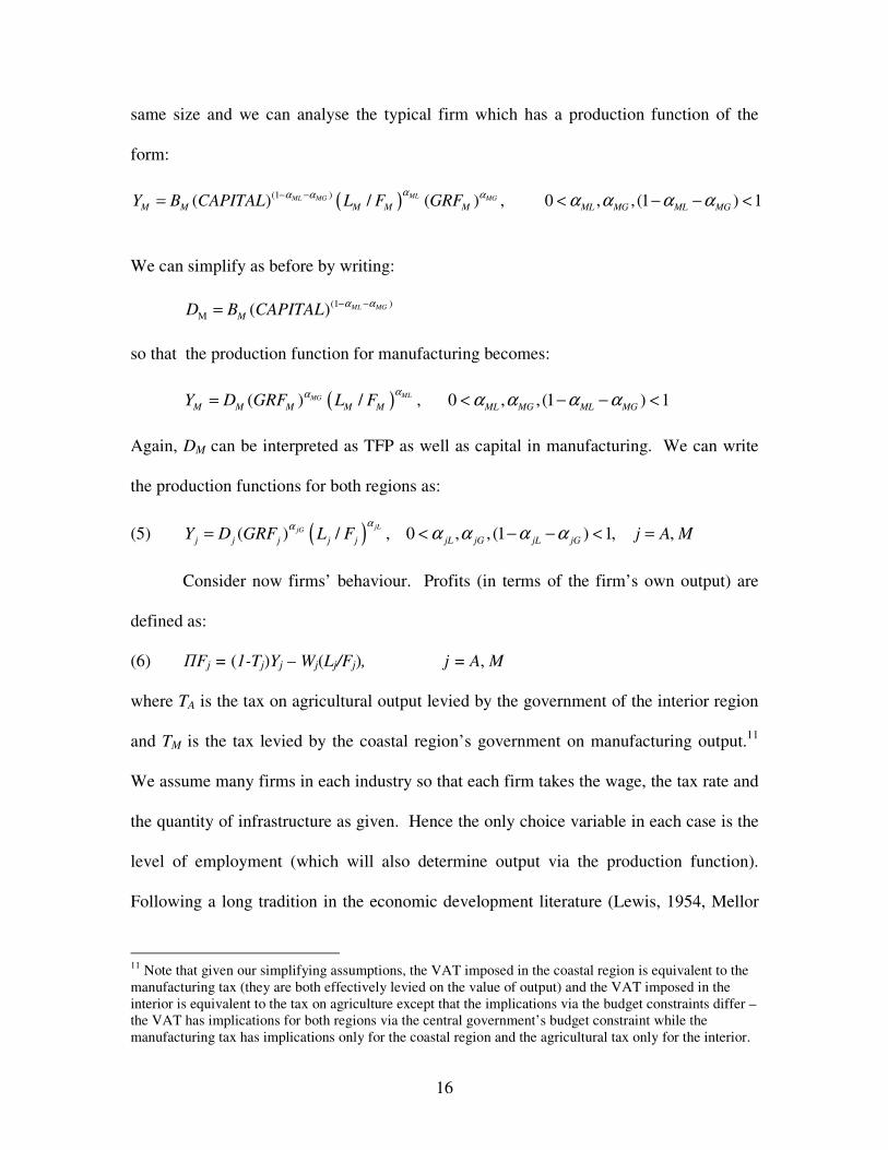
16

same size and we can analyse the typical firm which has a production function of the

form:

( ))(1( ) / ( ) , 0 , , (1 ) 1MLML MG MG

M M M M M ML MG ML MGY B CAPITAL L F GRFαα α α α α α α−−= < − − <

We can simplify as before by writing:

)(1

M ( ) ML MG

MD B CAPITAL

α α−−=

so that the production function for manufacturing becomes:

( )( ) / , 0 , , (1 ) 1MLMG

M M M M M ML MG ML MGY D GRF L F

αα α α α α= < − − <

Again, DM can be interpreted as TFP as well as capital in manufacturing. We can write

the production functions for both regions as:

(5) ( )( ) / , 0 , , (1 ) 1, ,jLjG

j j j j j jL jG jL jGY D GRF L F j A M

ααα α α α= < − − < =

Consider now firms’ behaviour. Profits (in terms of the firm’s own output) are

defined as:

(6) ΠFj = (1-Tj)Yj – Wj(Lj/Fj), j = A, M

where TA is the tax on agricultural output levied by the government of the interior region

and TM is the tax levied by the coastal region’s government on manufacturing output.11

We assume many firms in each industry so that each firm takes the wage, the tax rate and

the quantity of infrastructure as given. Hence the only choice variable in each case is the

level of employment (which will also determine output via the production function).

Following a long tradition in the economic development literature (Lewis, 1954, Mellor

11

Note that given our simplifying assumptions, the VAT imposed in the coastal region is equivalent to the

manufacturing tax (they are both effectively levied on the value of output) and the VAT imposed in the

interior is equivalent to the tax on agriculture except that the implications via the budget constraints differ –

the VAT has implications for both regions via the central government’s budget constraint while the

manufacturing tax has implications only for the coastal region and the agricultural tax only for the interior.

17

and Stevens, 1956, Gutman, 1957, Robinson, 1971, and Rey, 1998), we make different

behavioural assumptions for the two sectors – manufacturing firms in the coastal region

are assumed to choose employment to maximise profits but in the inland region all

workers are assumed to find employment in agriculture with the farm output being shared

equally among all workers. In agriculture, therefore, the wage is equal to the average

product and profits are zero.

The profit-maximising condition for manufacturing firms will result in the usual

marginal productivity condition:

(7a) ( )1

(1- ) ( ) / MLMG

M ML M M M M MT D GRF L F W

ααα−

=

In agriculture the assumption that labour is paid its average product results in the

following condition:

(7b) ( )1

(1- ) ( ) / ALAG

A A A A A AT D GRF L F W

αα −=

On the labour supply side, each household in each region is assumed to provide one unit

of labour inelastically to the firms in its own region so that labour force, labour supply,

employment and the number of households are all equal.

2.3 Governments

There are three sources of government revenue. The central government levies a

VAT at a uniform rate across the country and shares the revenue with the regional

governments. In addition, each regional government has its own tax: the coastal

government raises revenue through a business tax on manufacturing industry and the

inland government levies an agricultural tax on the value of farm output. Each

government (central, coastal and interior) receives tax revenue in the form of output and

18

costlessly transforms this output into a homogeneous government good. The central

government provides this to households as a consumption good in both regions, in per

capita amounts which are the same for all households within the region but may differ

across regions. Each regional government provides some output to households as a

consumption good (in equal per capita amounts) within its own region as well as

providing some to firms as infrastructure.

There are no assets in the model so that neither households, nor firms nor

governments can lend or borrow. Governments therefore must balance their budgets.

Consider the central government first. It raises VAT of NITVJI in region I and NCTVJC in

region C. Of this, a proportion (1-θ) is transferred to the regional governments and the

remainder is transformed costlessly into the government consumption good. In particular,

we assume that one unit of the composite good can be transformed into a unit of the

government good. The central government receives VAT revenue which is levied on

incomes which are measured in terms of the composite good. Its budget constraint

therefore has the simple form so that each unit of revenue is transformed into a unit of the

government good:

(8) NIGCI + NCGCC = θTV(NIJI+NCJC).

where GCi (i=I,C) is government good per household provided to residents of region i, TV

is the VAT rate and θ is the central government’s share of the VAT proceeds.

The regional governments receive some revenue from the VAT which is

measured in terms of the composite good but also some from local firms which is

measured in terms of the firm’s own output and is therefore re-valued in terms of the

19

composite good before being transformed into the government good. The regional

governments’ budget constraints have the form:

(9a) NIGRHI + GRFA = FATAP1-λ

YA+(1-θ)TVNIJI

(9b) NCGRHC + GRFM = FMTM P-λ

YM+(1-θ)TVNCJC

2.4 Aggregate variables and closure

It remains to introduce a number of important aggregate variables, definitions and

market-clearing conditions to complete the specification of the model.

First, the aggregate counterparts to the regional disparity variables are defined.

We begin with aggregate output.12

Recall that output is measured per firm so that to

compute national output we first compute regional output for each region, convert each

region’s output to the composite good before adding them:

(10) Y = FAP1-λ

YA + FMP-λ

YM

For income, we simply add total income (per capita income multiplied by population) of

each region since they are already measured in terms of the composite good:

(11) J = NIJI + NCJC

The appropriate procedure for welfare is less straightforward because of the problem of

comparing utilities. We overcome this at the regional level by assuming identical

households but households may differ across regions so that the same procedure is not

obviously correct. We decide to treat all individuals equally and simply measure national

12

Note that in much of the development literature, national development is measured using per capita

output or income. In our model, national population will be assumed to be constant so that per capita

output will always change equi-proportionately with aggregate output and similarly for income and welfare

so that aggregate and per capita variables may be used interchangeably to measure national development.

20

welfare as the population-weighted average of the utilities of the two types of identical

households:

(12) V = (NI/N)VI + (NC/N)VC.

Next, we introduce a number of definitions. First, the relationship between GHi

and its components is given by:

(13) GHi = GRHi + GCi, i = I, C

Second, as a matter of definition, wages in manufacturing are the same as the wage

received per household in the coastal region and the agricultural wage is the same as the

wage received by the representative interior household:

(14a) WI = WA

(14b) WC = WM

Market-clearing conditions are imposed on goods and labour markets. Goods-

markets clearing in each region implies:

(15a) FAYA = NICAI + NCCAC + TAFAYA+TVNIPλ-1

JI,

(15b) FMYM = NICMI + NCCMC + TMFMYM + TVNCPλJC

where we use the fact that in each case income is measured in terms of the composite

good while consumption and output are measured in terms of output of agricultural and

manufacturing goods. The labour market in each region clears so that employment in

agriculture is equal to the number of households in the interior region (each household

supplying one unit of labour) and the employment level in manufacturing is equal to the

number of coastal households:

(16a) LA = NI

(16b) LM = NC

21

Firms are assumed to distribute all their profits to households in their own region in equal

per capita amounts:

(17a) FAΠFA = NIΠHI,

(17b) FMΠFM = NCΠHC

The trade between regions must balance:

(18) NCPCAC = NICMI.

Finally, there is a given national population, N, which we assume to be exogenous

(19) NI + NC = N

To summarise, the model consists of the 33 equations, (1) to (19) in 44 variables:

Vi, Cji, GHi, P, Ji, ΠHi, Wi, Fj, Dj, Yj, Lj, Ni, ΠFj, TV, Tj, Wj, GRHi, GRFj, GCi, θ, N, µ, Y, J,

and V,

of which 13 are exogenous:

Fj, Dj, Tj, one of (GRHI, GRFA), one of (GRHC, GRFM), one of (GCI, GCC), θ, TV, N, and

µ,

so that there are 31 endogenous variables:

Vi, Cji, GHi, P, Ji, ΠHi, Wi, Yj, Lj, Ni, ΠFj, Wj, Y, J, V, one of (GRHI, GRFA), one of (GRHC,

GRFM) and one of (GCI, GCC).13

Two equations, however, are redundant since (3), (6), (14), (16), (17), (18) and the

household budget constraint can be used to derive (15) so that the balance between

number of equations and number of endogenous variables is restored.

13

Note that which of (GRHI, GRFA), for example, is chosen to be exogenous may affect the simulation

results. In some cases the choice will be clear, such as when we wish to compute the effect of a change in

GRHI in which case it must be the exogenous one. When we have a choice, we choose GRFA, GRFM and

GCC to be the exogenous variable in the three pairs in the list above. We will comment on the effects of

these choices in our discussion of the results. Note also that, strictly-speaking we should include the two Aj

as variables and declare them exogenous. But since they are areas of the two regions and there seems no

possible exercise which would require shocks to them, we treat them as parameters.

22

2.5 Short-run and long-run versions of the model

In the simulations to be reported below we distinguish between short-run and

long-run versions of the model. Since the model is static rather than dynamic, the

distinction is not based on the notion of equilibrium but corresponds, as in many CGE

models, to differences in closure assumptions. In particular, we define the short run as

the length of time before inter-regional migration begins to respond to the changes in VI

and VC. The distinction is based on the idea that migration is slow to respond fully to

changes in economic incentives. Thus, for example, Pissarides and McMaster (1990)

estimate that it takes as long as 20 years for reasonably complete adjustment of migration

to labour-market shocks. In terms of the model, this simply involves suspending

equations (4) and (19) and making NI and NC exogenous in the simulation. The long run

is used to refer to the simulation results using the model as set out above.

2.6 Linearising the model

The model as it stands is too complicated to solve analytically so that we

linearise it in terms of proportional changes for which we use a process of log

differentiation. This converts the model from one which is non-linear in the levels to one

which is linear in the proportional rates of change of the variables. The resulting

linearised versions of equations (1)-(19) are given in Appendix 2.

2.7 The numerical version of the linearised model

Having linearised the model in terms of proportional changes, we can solve the

model for any one of the (changes in the) endogenous variables in terms of (the changes

23

in) the exogenous variables. However, given the number of endogenous variables, this is

unlikely to lead to any interpretable results and we proceed to solve the model

numerically using data for China’s regions to calibrate the key parameters of the model,

detailed discussion of which we relegate to Appendix 3.

3. The Simulations

Given the number of exogenous variables in the model, there are many possible

policies which might affect the regional distribution of output. We simulate four such

policy actions, which the interior government and central government might undertake to

reduce regional disparities and assess the effects on the disparities themselves and

examine whether there is a trade-off between the reduction of disparities and national

development. We examine three alternative disparity measures (output, income and

welfare) and their corresponding aggregate levels to assess the nature of the trade-off.

We consider two policies carried out by the regional government. They are:

(i) A regional government fiscal policy. The model structure provides various

possible balanced-budget fiscal policy combinations. We choose an increase in

interior government-provided consumption aimed at increasing both welfare and

expenditure and hence output via the usual multiplier effects in the region. We

assume that the interior government’s budget is balanced by changing the

provision of infrastructure. Alternatives involve the use of changes in taxation to

balance the regional government’s budget constraint and we comment briefly on

these as appropriate.

24

(ii) Measures which increase productive capacity in the agriculture sector, such as

releasing more land for agriculture or improving agricultural technology It might

be argued that there is little additional land available for release to agriculture in

China. However, the shock here may also be thought of as the implementation of

policy which halts or slows down the alienation of farm land for non-agricultural

purposes.

Policies which the central government might undertake to reduce disparities are:

(iii) A cut in hukou cost which makes migration from the interior to the coast cheaper.

We note that originally the hukou system was instituted and administered by the

central government but that since reforms began in the late 1970s it has

increasingly been the wealthier coastal provinces which have maintained the force

of the hukou restrictions, presumably to keep out low-wage workers from the poor

inland provinces. Coastal provinces are, therefore, hardly likely to undertake

reform or allow relaxation of the migration restrictions to benefit the poorer

inland provinces and it must be assumed that only the central government is likely

to apply pressure to reduce restrictions which make it costly for labour to move

from the interior provinces to the more prosperous coastal region.

(iv) A fiscal redistribution in the form of an increase in expenditure on the

consumption good in the interior region by the central government balanced by a

reduction in that in the coastal region to balance the government’s budget. An

alternative version of this policy is to change the VAT-sharing arrangements in

favour of the interior. Given the simple model structure, this turns out to have the

25

same qualitative effects as the expenditure change and we do not consider it

separately.

4. Results

4.1 Base case

A summary of the base case simulation results are included in Table 1. Detailed

results for all variables are reported in Appendix 4. We discuss the four policies in turn.

[Table 1 about here]

Policy 1: An interior government fiscal policy

Table 1 shows that policy 1 has the desired effect of reducing the income and welfare

gaps but that it increases the output per capita disparity in both the short and long runs.

Moreover, while there is a reduction in the income and welfare gaps, this is obtained at

the expense of a reduction in national welfare, income and output. Thus, in both short

and long runs, there is a trade-off when the measure of interest is income or welfare while

if policy targets output per capita, there is a deterioration in both the gap and the national

level.

The mechanism underlying these results is that the increase in government-

provided consumption expenditure in the interior region requires a decrease in

expenditure on government-provided infrastructure if the government is to maintain its

budgetary balance. The decrease in infrastructure reduces both output and per capita

output in the interior, the direct result of which is an increase in the output per capita gap

and a decrease in national output. The effect in the interior spills over into the coastal

region via relative price changes and inter-regional trade. The fall in interior output

26

increases agricultural prices relative to manufacturing prices. This results in a increase in

income in the interior region and a decrease in income in the coastal region (both of

which are valued in terms of composite good). These income changes reinforce the direct

effects of the policy of reducing the welfare gap between the interior and coastal regions.

For the country as a whole, the increases in income and welfare in the interior region are

not large enough to offset the corresponding decreases in the coastal region, so that the

reduction of the income and welfare gaps comes at the expense of lower income and

welfare nationally.

In the long run, the improvement in welfare in the interior relative to that in the

coast induces migration from the coast to the interior. This causes a fall in the output in

the coastal region and a further fall in output for the nation as a whole and partly reverses

the original increase in the relative price of agricultural goods and so partly reverses the

original effects on the welfare and income gaps. Indeed, welfare and income in the

interior both fall by a small amount in the long run.14

However, these long-run changes

are not large enough to reverse the direction of policy effects on the gaps: the income and

welfare gaps still decrease in the long run (although not by as much as in the short run)

and the gap in output per capita still increases while at the national level income, welfare

and output all fall in the long run.

14

Note that output in the interior falls further in the long run even though there is migration from the coast

to the interior. The full results for this case reported in the Appendix show that this is largely a government

budget effect: as noted in the text, in modelling the present policy shock, we assume that infrastructure

expenditure is the endogenous variable in the regional government’s budget constraint. An influx of

population requires the interior government to increase consumption expenditure to maintain this at the new

higher level, requiring a further fall in the level of infrastructure expenditure which reduces interior output

by more than enough to offset the beneficial effects of the increase in labour input.

27

There is therefore a trade-off in the income and welfare dimensions in both the

short and long runs and no trade-off in terms of output (in the sense that the policy

worsens both the per capita output gap and national output).

As mentioned in the previous section, alternative forms of regional government

fiscal policy are possible. An expansion of infrastructure spending balanced by a

reduction in the amount of the consumption good provided will, not surprisingly, have

the opposite effect of the policy just described – it will boost national levels of output,

income and welfare and reduce the per capita output gap but all this comes at the cost of

widening income and welfare gaps. Alternatively, increases in expenditure can be

balanced by a rise in the agricultural tax. These alternatives will have effects not

dissimilar to those just described with the dominant effect working through the change in

infrastructure spending.

In summary, regional government fiscal policy generally faces a trade-off in the

income and welfare dimensions but not in the output dimension.

Policy 2: An increase in agricultural productive capacity

Table 1 indicates that policy 2 is clearly effective in reducing the regional per

capita output gap and that it is also beneficial for national output growth both in the short

run and long run since the boost to agricultural productive capacity greatly increases

agricultural output in the interior region while leaving manufacturing output unchanged

in the short run and reducing it slightly in the long run. Thus, on the output front, there is

no trade-off between tackling inter-regional disparities and maintaining the level of

aggregate activity.

28

The increase in agricultural output, however, adversely affects its relative price

which means that income in the interior region actually decreases while that in the coastal

region increases, which worsens the income gap between the two regions. But the income

fall in the interior region is smaller than the increase in the coast so that national income

increases. Similarly, welfare in the interior falls while that in the coast increases so the

welfare gap increases but national welfare also increases since the fall in the interior is

more than offset by the change in the opposite direction in the coast. Thus, as with

regional government fiscal policy, there is a trade-off when the government targets

welfare or income.

In the long run, the utility difference induces migration from the interior region to

the coast, which increases income in the interior (resulting both from the increase in

wages and profits in the interior region and from the relative price change which is now

in favour of the agricultural good) and welfare in the interior but not by enough to reverse

the short-run adverse effects on the welfare and income gaps although national income

and welfare continue to improve. Thus in the long run welfare, income and output all

increase in both regions but output per capita falls in the coastal region due to a modest

movement of population to the coast which increases output but, with decreasing

marginal product of labour, reduces output per capita. Despite the generally beneficial

effects on both regions, the inter-regional welfare and income gaps both widen (while

difference between output per capita in the two regions narrows). As with regional fiscal

policy, there is a trade-off between equality and national development in the income and

welfare dimensions but not as far as output is concerned.

29

Policy 3: A relaxation of the hukou restrictions

Table 1 shows that policy 3 has no effects in the short run which is not surprising

since the internal migration channel through which it operates is closed in the short run.

However, in the long run the hukou relaxation induces substantial migration from the

interior to the coastal region, which reduces the output in the interior while increasing

both the coastal output and national output. Given declining marginal productivity of

labour, the fall in output in the interior is less than the fall in labour inputs so that per

capita output increases in the interior region. For the same reason, per capita output in the

coastal region is falls. Therefore, policy 3 unambiguously narrows the regional per capita

output gap. It also increases national output since the coastal expansion more than offsets

the interior contraction. There is therefore no trade-off in the output dimension.

Policy 3 is also helpful in reducing the regional income and welfare gaps in the

long run. The mechanism is that the outflow of labour from the interior region improves

wages and profits in the interior region and the reduction in output in the interior region

has a relative price effect in favour of the agricultural good, both of which serve to

increase income in the interior. The increase in income in the interior has positive effects

on welfare in this region, which also benefits from the outflow of labour since this results

in an increase of the government-provided consumption good (both because of the rise in

the per capita tax base and an increase in the tax revenue from the VAT). On the contrary,

the inflow of migration into the coastal region is harmful for the utility and income of the

representative household in this region. However, since the decrease in income and utility

in the coastal region is smaller than the increase in the interior region, national income

30

and welfare both increase so that the government avoids a trade-off in the income and

welfare dimensions.

Thus, policy 3 is the first of the three policies considered so far for which there is

not trade-off for any of the three variables considered: income, welfare and output.

However, while appearing beneficial in all dimensions, the coastal region becomes

worse-off (per capita output, welfare and income all fall), making it likely that the coastal

government(s) will strongly oppose relaxation of migration restrictions.

Policy 4: A fiscal redistribution by the central government

As stated in the previous section, the structure of the model allows us to define at

least two fiscal redistribution policies, one an expansion of expenditure in the interior

matched by a reduction in the coast and the other a change in the VAT-sharing

arrangements in favour of the interior. Both have qualitatively similar effects and we

focus on the first – a rise in the provision of the government consumption good to the

interior with the central government’s budget being balanced by a fall in the provision of

the good to the coastal residents.

Table 1 shows that policy 4 has short-run effects only on welfare. Its effects on

the welfare in the interior is positive while its effect on the welfare in the coastal region is

negative which simply reflects the redistribution from the coast to the interior. Although

the coastal utility loss is smaller than the interior’s utility gain, national welfare falls

because of the greater coastal population.

Over time, people move from the coast to the interior in response to the welfare

gap. The inflow of labour into the interior increases the output in this region and

31

decreases that in the coastal region also decreasing national output. As in previous cases,

per capita output moves in the opposite direction so that the regional per capita output

gap increases. Relative prices move against agriculture which has a negative effect on

income in the interior region and also on national income. The inflow of migration into

the interior region also reduces the short-run welfare benefits to that region and so

mitigates the short-run policy effects of reducing the regional welfare gap.

Therefore, policy 4 has some benefits in reducing the regional welfare gap but it

enlarges the regional income and per capita output gaps and reduces national income,

welfare and output. The central government therefore faces a trade-off in the welfare

dimension in both the short and long runs but no trade-off in the output and income

dimensions.

4.2 Sensitivity to calibration of the substitution elasticity

In CGE modelling in general the elasticity of substitution is an important

parameter and, moreover, it is difficult to calibrate (see, e.g., Mansur and Whalley, 1984).

In our analysis we use a CES utility function so that the elasticity of substitution in

consumption between the agricultural and manufacturing goods is potentially an

important parameter in the model since it is likely to influence relative price changes

which have featured centrally in our explanation of the effects of policy shocks,

particularly the effects on income. As pointed out in Appendix 3, in calibrating the

model we use an average value of others’ econometric estimates of the substitution

elasticity. To assess the sensitivity of the results reported above to this choice, we re-ran

32

the simulations with the low and high values for the substitution elasticity. Our base-case

results use a value of 0.44 and Appendix 5 reports results for values of 0.2 and 0.68.

As expected, the value of substitution elasticity does have some effects on the

results, particularly on the income effects which, in turn, affect utility and, in the long run,

output though the channel of migration. The results reported in Appendix 5 show that the

smaller the value of the substitution elasticity, the larger the effect of policy shocks on

income. The mechanism is that the smaller the substitution elasticity, the more difficult is

substitution between agricultural goods and manufacturing goods and so the larger the

relative price change, which affects income in both regions. However, the direction of

change in disparities (income, welfare and per capita output) and of the change in

national variables (output, income and welfare) are not affected by the different

elasticities experimented with so our main conclusions regarding the existence of trade-

off are not undermined.

5. Conclusions

The focus of this paper is the tension between reducing inter-regional disparities

and maintaining the level of aggregate activity – is there a cost in terms of national

development foregone when policies to reduce inter-regional gaps are implemented? Our

starting point was that both regional- and national-level variables are likely to be

endogenous in any satisfactory regionally-disaggregated macro model so that whether an

inter-regional gap and the corresponding national variable move together or in opposite

directions will, in general, depend on the shock imposed on the model.

33

To explore this issue, we built a small two-region model capturing some of the

characteristics of the Chinese economy and subjected it to a number of shocks of which

we described four in detail. The effects of these shocks on inter-regional gaps in per

capita output, income and welfare as well as on the corresponding national levels of these

variables were analysed using simulations of a numerical version of the model.

Given that the signs of the effects of policy shocks are of most relevance for the

question at hand, we summarise these signs in Table 2. We consider three gaps: in per

capita output, income and welfare as well as the aggregate counterparts to these variables.

Two broad conclusions may be drawn from the information in the table.

[Table 2 about here]

First, different gaps generally move in different directions so that policy-makers

need to be clear as to which gap is being targeted. For the two policies initiated by the

regional government the welfare and income gaps move together but in the opposite

direction to the gap in per capita output. For the central government redistribution policy

it is the gaps in per capita output and income which move together in the opposite

direction to welfare. Finally, only in the policy which reduces inter-regional migration

costs, do all three gaps move in the same direction.

Second, whether a narrowing of the gap between the interior and the coast comes

at the expense of the national level of the relevant variable depends also on the shock. In

particular, regional government fiscal and productivity policies face a trade-off in both

welfare and income dimensions, central government redistribution policy faces a trade-

off in the welfare dimension only and while the hukou policy alone faces no trade-off at

all.

34

In summary, whether a trade-off exists generally depends on both the variable of

interest and on the nature of the policy shock. Fiscal redistribution policies always face a

trade-off in at least one dimension and often in two. Only a reduction of the costs of

internal migration reduces the inter-regional disparities for all three variables considered

– income, welfare and per capita output – and does so while increasing the national level

of these variables, thus producing both inert-regional and national benefits. But even this

policy comes at a cost – the coastal region loses in terms of welfare, income, and output

per capita and can, on the basis of these results, be expected to continue to oppose a

relaxation of the restrictions on internal migration in China.

35

References

Alesina, A. and D. Rodrik (1994), “Distributive Politics and Economic Growth”,

Quarterly Journal of Economics, 109, 465-490.

Bao, S., G. H. Chang, J. D. Sachs and W. T. Woo (2002) “Geographic Factors and

China's Regional Development under Market Reforms, 1978–1998”, China

Economic Review, 13, 89-111.

Barro, Robert J. (2000), “Inequality and Growth in A Panel of Countries”, Journal of

Economic Growth, 5, 87-120.

Barro, Robert J. (2008), “Inequality and Growth Revised”, Asian Development Bank

Working Paper Series on Regional Economic Integration No.11.

Benabou, R.(1996), “Inequality and Growth”, In: Bernanke, Ben S., Rotemberg, Julio J.

(Eds.), NBER Macroeconomics Manual, MIT Press, Cambridge, MA.

Benhabib, J. and A. Rustichini (1996), “Social Conflict and Growth”, Journal of

Economic Growth, 1, 129–146.

Boadway, R. and Flatters, F. (1982), “Efficiency and Equalisation Payments in a Federal

System of Government: A Synthesis and Extension of Recent Results”, Canadian

Journal of Economics, 15, 613-633.

Bjornskov, C. (2008), “The Growth-Inequality Association: Government Ideology

Matters”, Journal of Development Economics, 87, 300-308.

Brun, J.F., J. L. Combes and M. F. Renard (2002), “Are there Spillover Effects between

the Coastal and Noncoastal Regions in China?”, China Economic Review, 13,.

161-169.

Chambers, D. (2007), “Trading Places: Does Past Growth Impact Inequality?”, Journal of

Development Economics, 82, 257-266.

Chang, J. Y. and Ram, R. (2000), “Level of Development, Rate of Economic Growth and

Income Inequality”, Economic Development and Cultural Change, 48(4), 787-799.

Cheng, T. and Selden, M. (1994), “The Origins and Consequences of China’s Hukou

System”, The China Quarterly, 139, 644-668.

Demurger, S. (2001), “Infrastructure Development and Economic Growth: An

Explanation for Regional Disparities in China?”, Journal of Comparative

Economics, 29, 95-117.

Easterly, W. (2007), “Inequality Does Cause Underdevelopment: Insights from a New

Instrument”, Journal of Development Economics, 84, 755-776.

Edin, P. A. and Topel, R. (1997), “Wage Policy and Restructuring: the Swedish Labor

Market since 1960”, in Freeman , R.B., Topel, R., Swedenborg, B.(eds), The

Welfare State in Transition, Reforming the Swedish Model, University of

Chicago Press, Chicago, pp155-201.

Fallah, B. and Partridge, M. (2007), “The Elusive Inequality-Economic Growth

Relationship: Are There differences between Cities and the countryside?”, Annals

of Regional Science, 41, 375-400.

Fan, S. (1991), “Effects of Technological Change and Institutional Reform on Production

Growth in Chinese Agriculture”, American Journal of Agricultural Economics, 73,

266-275.

36

Fleisher, B. M and J. Chen (1997), “The Coast-Noncoast Income Gap, Productivity and

Regional Economic Policy in China”, Journal of Comparative Economics, 25,

220-236.

Forbes, Kristin J. (2000), “A Reassessment of the Relationship between Inequality and

Growth”, American Economic Review, 90, 869–887.

Fujita, M. and Hu, D. (2001), “Regional disparity in China 1985-1994: The effects of

globalization and liberalization”, Annals of Regional Science, 35, 3-37.

Galor, O. and J., Zeira (1993), “Income Distribution and Macroeconomics”, Review of

Economic Studies, 60, 35-52.

Golley, J. (2007), The Dynamics of Chinese Regional Development: Market Nature, State

Nurture, Edward Elgar Publishing Ltd, Cheltenham, UK.

Groenewold, N., A Chen and G. Lee (2008), Linkages between China’s Regions:

Measurement and Policy, Edward Elgar, Cheltenham, UK.

Groenewold, N. and Hagger, A. J. (2005), “The Effects of an Inter-Regional Transfer

with Empire-Building Regional Governments”, Review of Regional Studies, 35,

38-63.

Groenewold, N. and Hagger, A. J. (2007), “The Effects of Fiscal Equalisation in a Model

with Endogenous Regional Governments: An Analysis in a Two-Region

Numerical Model”, Annals of Regional Science, 41, 353-374.

Groenewold, N., Hagger, A. J. and Madden, J. R. (2000), “Competitive Federalism: A

Political-Economy General Equilibrium Approach”, Australasian Journal of

Regional Science, 6, 451-465.

Groenewold, N., Hagger, A. J. and Madden, J. R. (2003), “Interregional Transfers: A

Political-Economy CGE Approach”, Papers in Regional Science, 82, 535-554.

Gutman, G. O. (1957), "A Note on Economic Development with Subsistence

Agriculture", Oxford Economic Papers, 9, 323-334.

He, C., Wei, Y. D. and X. Xie (2008), ‘Globalization, Institutional Change, and Industrial

Location: Economic Transition and Industrial Concentration in China’, Regional

Studies, 42, 923-945.

Hertel, T. and Zhai, F. (2006), “Labour Market Distortions, Rural-Urban Inequality and

the Opening of China’s Economy”, Economic Modelling, 23, 76-109.

Hirschman, A. (1958), The Strategy of Economic Development, New Haven: Yale

University Press.

Hu, D.(2002), “Trade, Rural–Urban Migration, and Regional Income Disparity in

Developing Countries: A Spatial General Equilibrium Model Inspired by the Case

of China”, Regional Science and Urban Economics, 32, 311–338.

Jin, H., Qian, Y. and Weingast, B. R. (2005), “Regional Decentralization and Fiscal

Incentives: Federalism Chinese Style”, Journal of Public Economics, 89, 1719-

1742.

Jin, J. and H. Zou (2005), “ Fiscal Decentralization, Revenue and Expenditure

Assignments and Growth in China”, Journal of Asian Economics, 16, 1047-1064.

Kaldor, N., 1956, “Alternative Theories of Distribution”, Review of Economic Studies,23,

83-100.

Kuijs, L. and T. Wang (2005), "China's Pattern of Growth: Moving to Sustainibility and

Reducing Inequality", World Bank China Research Paper, No.2.

37

Kuznets, S. (1955), “Economic Growth and Income Inequality”, American Economic

Review, 45, 1-28.

Lewis, W. A. (1954), “Economic Development with Unlimited Supplies of Labour”,

Manchester School of Economic and Social Studies, 22, 139-191.

Li, C. (2009), “Savings, Investment and Capital Mobility within China”, China Economic

Review, doi:10.1016/j.chieco.2009.08.005.

Li, S. and J., He (2006), “China’s Economic Development Prospects (2006-2020)”, paper

presented at the ACE International Conference in Hong Kong.

Liu, Z. (2005), “Institution and Inequality: The Hukou System in China”, Journal of

Comparative Economics, 33, 133-157.

Lundberg, M. and L. Squire (2003), “The Simultaneous Evolution of Growth and

Inequality”, Economic Journal, 113, 326-344.

Mansoorian, A. and Myers, G.M.(1993), “Attachment to Home and Efficient Purchases

of Population in a Fiscal Externality Economy”, Journal of Public Economics, 52,

117–132.

Mansur, A., Whalley, J.(1984), “Numerical Specification of Applied General Equilibrium

Models: Estimation, Calibration and Data”, in Scarf, H.E. and Shoven, J.B. (eds.)

Applied General Equilibrium Analysis, Cambridge University Press, Cambridge.

Mellor, J. W. and Stevens, R. D. (1956), “The Average and Marginal Product of Farm

Labor in Underdeveloped Economies”, Journal of Farm Economics, 38, 780-791.

Myers, G. M. (1990), “Optimality, Free Mobility and the Regional Authority in a

Federation”, Journal of Public Economics, 43, 107-121.

Myrdal, G. (1957), Economic Theory and Underdeveloped Regions, London: Duckworth.

Partridge, M.(2005), “Does Income Distribution effect US State Economic Growth?”,

Journal of Regional Science, 45, 363-394.

Persson, T. and G., Tabellini (1994), “Is Inequality Harmful for Growth?”, American

Economic Review, 84, 600-621.

Petchey, J. (1993), “Equalisation in a Federal Economy with Inter-State Migration and

Different Factor Endowments”, Australian Economic Papers, 32, 343-353.

Petchey, J. (1995), “Resource Rents, Cost Differences and Fiscal Equalization”,

Economic Record, 71, 343-353.

Petchey, J. and Shapiro, P. (2000), “The Efficiency of State Taxes on Mobile Labour

Income”, Economic Record, 76, 285-296.

Pissarides, C.A. and I. McMaster (1990), “Regional Migration, Wages and Unemployment:

Empirical Evidence and Implications for Policy”, Oxford Economic Papers, 42, 812-

831.

Poncet, S. (2006), “Provincial Migration Dynamics in China: Borders, Costs and

Economic Motivations”, Regional Science and Urban Economics, 36, 385-398.

Qiao, B, Martinez-Vazquez, J. and Xu, Y. (2008), “The Trade-off Between Growth and

Equity in Decentralisation Policy: China’s Experience”, Journal of Development

Economics, 86, 112-128.

Rey, D. (1998), Development Economics, Princeton University Press, Princeton, NJ.

Robinson, W. C. (1971), “The Economics of Work Sharing in Peasant Agriculture”,

Economic Development and Cultural Change, 20, 131-141.

38

Shen, C., Jin, J. and Zou, H. (2006), “Fiscal Decentralization in China: History, Impacts,

Challenges and Next Steps”, World Bank Discussion Paper.

State Statistical Bureau (2005), China Civil Affairs Statistical Yearbook 2005, Statistical

Publishing House of China, Beijing.

State Statistical Bureau (2007), China Statistical Abstract 2007, Statistical Publishing

House of China, Beijing.

State Statistical Bureau (various issues), Statistical Yearbook of China, Statistical

Publishing House of China, Beijing.

Tochkov, K. (2007), “Interregional Transfers and the Smoothing of Provincial

Expenditure in China”, China Economic Review, 18, 54-65.

Wan G., M. Lu and Z. Chen (2006), “The Inequality–Growth Nexus In the Short and

Long Run: Empirical Evidence from China”, Journal of Comparative Economics,

34, 654-667.

Whalley, J. and Zhang, S. (2007), “A Numerical Simulation Analysis of (Hukou) Labour

Mobility Restrictions in China”, Journal of Development Economics, 83, 392-410.

Williamson, J. (1965), “Regional Inequality in the Process of National Development”,

Economic Development and Cultural Change, 17, 3-84.

Woodland, A.D. and Yoshida, C.(2006),“Risk Preference, Immigration Policy and Illegal

Immigration”, Journal of Development Economics, 81, 500– 513.

Zhang, T. and Zou, H. (1998), “Fiscal Decentralization, Public Spending and Economic

Growth in China”, Journal of Public Economics, 67, 221-240.

Zhang, X. (2006), “Fiscal Decentralization and Political Centralization in China:

Implications for Growth and Inequality”, Journal of Comparative Economics, 34,

713-726.

Zhang, Y. and Zou, H. (2001), “The Growth Impact of Intersectoral and

Intergovernmental Allocation of Public Expenditure: With Applications to China

and India”, China Economic Review, 12, 58-81.

Zhang, Z. and Martinez-Vazquez, J. (2003), “The System of Equalizing Transfers in

China”, International Studies Program Working Paper 03-12, Andrew Young

School of Policy Studies, Georgia StateUniversity.

39

Table 1 Summary of Base Case Simulation Results

Policy 1 Policy 2 Policy 3 Policy 4 Variables

SR LR SR LR SR LR SR LR

vI 0.0778 -0.0476 -0.1574 0.2567 0.0000 0.5256 0.1619 0.0611

vC -0.2483 -0.2181 1.0246 0.7293 0.0000 -0.3747 -0.1296 -0.0580

v -0.1737 -0.2383 0.7544 0.7854 0.0000 0.0393 -0.0630 -0.0722

jI 0.1179 -0.0242 -0.4864 0.0079 0.0000 0.6274 0.0000 -0.1246

jC -0.2716 -0.2288 1.1209 0.7707 0.0000 -0.4444 0.0000 0.0883

j -0.0983 -0.1601 0.4059 0.4933 0.0000 0.1109 0.0000 -0.0220

yA -0.2423 -0.2987 1.0000 0.9499 0.0000 -0.0636 0.0000 0.0126

yM 0.0000 -0.0654 0.0000 0.1813 0.0000 0.2301 0.0000 -0.0457

y -0.1042 -0.1657 0.4299 0.5117 0.0000 0.1038 0.0000 -0.0206

lA 0.0000 0.0723 0.0000 -0.2005 0.0000 -0.2544 0.0000 0.0505

lM 0.0000 -0.0982 0.0000 0.2721 0.0000 0.3453 0.0000 -0.0686

p 0.6317 0.6084 -2.6073 -2.0039 0.0000 0.7657 0.0000 -0.1521

yA-lA -0.2423 -0.3711 1.0000 1.1504 0.0000 0.1908 0.0000 -0.0379

yM-lM 0.0000 0.0328 0.0000 -0.0908 0.0000 -0.1152 0.0000 0.0229

Notes: since yj and lj are log differences of output and population respectively, yj-lj is the log difference of

output per capita. Policy 1 has grhi = 1 and grfj endogenous; policy 2 has dj =1 and grhi endogenous,

policy 3 has µi = 1 and grhi endogenous, policy 4 has gcI = 1 and gcC endogenous.

Table 2: Summary of results

Policy 1 Policy 2 Policy 3 Policy 4 Variables

SR LR SR LR SR LR SR LR

welfare gap - - + + 0 - - -

income gap - - + + 0 - 0 +

Pc output gap + + - - 0 - 0 +

aggregate welfare - - + + 0 + - -

aggregate income - - + + 0 + 0 -

aggregate output - - + + 0 + 0 -

Note: . Policy 1 has grhi = 1 and grfj endogenous; policy 2 has dj =1 and grhi endogenous, policy 3 has µi

= 1 and grhi endogenous, policy 4 has gcI = 1 and gcC endogenous.

40

Figure 1 The two regions of mainland China

41

Appendix 1: Definition of variables

Vi = utility of the representative household, region i,

V = national welfare,

CAi = real private consumption of agricultural output per household, region i,

CMi = real private consumption of manufactured good per household, region i,

GHi = real government-provided consumption per household, region i.

P = price of agricultural good in terms of manufactured good

Ji = real household income (net of VAT), region i,

J = national income,

ΠHi = real profit distribution per household, region i

Wi = real wage income per household, region i

Fj = the number of firms, sector j

Dj = productivity parameter, sector j

Yj = real output, sector j

Y = national output,

Lj = employment, sector j

Ni = population, region i

ΠFj = firm profit, sector j

Tv = value added tax rate

Tj = output tax rate, sector j

Wj = real wage income, sector j

GRHi = real regional government-provided consumption good per household, region i

GRFi = real regional government-provided public good, region i

GCi = real central government-provided consumption good per household in region i

θ = share of valued tax to the central government

N = national population

µ = hukou parameter

Appendix 2: Linearised version of the model

The model of section 2 is linearised in terms of proportional differences by taking

logarithms and differentials of each equation. The linearised form of equations (1) to (19)

(excluding equations (15) which are redundant) of the model are as follows, with the

linearised form having the same number as the original equation but being distinguished

by a prime.

The linearised utility function is:

(1’) i caiv Ai cmiv Mi ghiv i

v c c ghσ σ σ= + + i=I, C

where lower-case letters represent the proportional changes (log differential) of their

upper-case counterparts and

Ai Aicaiv

Ai Ai Mi Mi i i

C

C C GH

ρ

ρ ρ ρ

γσ

γ γ δ

−

− − −=

+ +,

Mi Micmiv

Ai Ai Mi Mi i i

C

C C GH

ρ

ρ ρ ρ

γσ

γ γ δ

−

− − −=

+ +,

i ighiv

Ai Ai Mi Mi i i

GH

C C GH

ρ

ρ ρ ρ

δσ

γ γ δ

−

− − −=

+ +.

42

The linearised consumption demand functions are:

(2a’) Ai i cai elas

c j p p pλ σ σ= + − − i=I, C

where 1

1 1

1

1 ( )

cai

Mi

Ai

P

ρ

ρ ρ

ρ

ρσ

γ

γ

−

+ +

+=

+

, 1

1elas

σρ

=+

, and

(2b’) Mi i cai

c j p pλ σ= + − i=I, C.

The linearised definitions of real household income are:

(3a’) (1 )tv v I hjI I wjI It j p h wπσ λ σ π σ+ = − + +

where IhjI

I I

H

H Wπσ

Π=

Π +, I

wjI

I I

W

H Wσ =

Π +,

1

vtv

v

T

Tσ =

+, and

(3b’) tv v C hjC C wjC Ct j p h wπσ λ σ π σ+ = − + +

where ChjC

C C

H

H Wπσ

Π=

Π +, C

wjC

C C

W

IIH Wσ =

+.

The linearised migration equilibrium condition corresponding to equation (4) is:

(4’) /

* log( ) ( )/

C CC I C I

I I

N Av v n n

N Aµ µ µ= + + −

where µ* = dµ/µ and we have used the obvious assumption that area is constant.

The linearised production functions are:

(5’) ( )j j jG j jL j j

y d grf l fα α= + + − j=A, M.

The linearised profit definitions are given by:

(6’) ( )j y fj j tj y fj j w fj j j j

f y t w l fπ π ππ σ σ σ σ= − − + − j=A, M

where (1 )

,j j

y fj

j

T Y

Fπσ

−=

Π

1

j

tj

j

T

Tσ =

−,

( / )j j j

w f j

j

W L F

Fπσ =

Π.

The manufacturing sector’s profit-maximisation condition in linear form is:

(7a’) (1 )( ) 0M tM M M MG M ML M M

w t d grf l fσ α α+ − − + − − =

and that for agriculture is given by:

(7b’) (1 )( ) 0A tA A A AG A AL A A

w t d grf l fσ α α+ − − + − − = .

The central government’s budget constraint is linearised as:

(8’) ( ) ( ) * ( ) ( )gcIgc I I gcCgc C C v jIj I I jCj C C

n gc n gc t n j n jσ σ θ σ σ+ + + = + + + + +

where I IgcIgc

I I C C

N GC

N GC N GCσ =

+, C C

gcCgc

I I C C

N GC

N GC N GCσ =

+, I I

jIj

I I C C

N J

N J N Jσ =

+,

C CjCj

I I C C

N J

N J N Jσ =

+, θ* = dθ/θ.

The regional government’s budget constraint in linear form is given by:

(9a’) ( )grhIgr I I grfAgr A

n grh grfσ σ+ +

( ) ( * )tAgr A A A tvIgr V I I

f t p p y t n jθσ λ σ σ θ= + + − + + − + + +

43

where I IgrhIgr

I I A

N GRH

N GRH GRFσ =

+, A

grfAgr

I I A

GRF

N GRH GRFσ =

+,

1θ

θσ

θ=

−,

1

1 (1 )

A A AtAgr

A A A V I I

F T P Y

F T P Y T N J

λ

λσ

θ

−

−=

+ −,

1

(1 )

(1 )

V I ItvIgr

A A A V I I

T N J

F T P Y T N Jλ

θσ

θ−

−=

+ −, and

(9b’) ( )grhCgr C C grfMgr Mn grh grfσ σ+ +

( ) ( * )tMgr M M M tvCgr V C Cf t p y t n jθσ λ σ σ θ= + − + + − + + +

where C CgrhCgr

C C M

N GRH

N GRH GRFσ =

+, M

grfMgr

C C M

GRF

N GRH GRFσ =

+,

(1 )

M M MtMgr

M M M V C C

F T P Y

F T P Y T N J

λ

λσ

θ

−

−=

+ −,

(1 )

(1 )

V C CtvCgr

M M M V C C

T N J

F T P Y T N Jλ

θσ

θ−

−=

+ −.

The definition of national output is linearised as:

(10’) ( ) ( )yyA A A yyM M M

y f y f yσ σ= + + +

where AyyA

A M

Y

Y Yσ =

+, M

yyM

A M

Y

Y Yσ =

+ and we assume that

yyAλ σ= .

The definition of national income is linearised as:

(11’) ( ) ( )nIj I I nCj C C

j j n j nσ σ= + + +

where I InIj

I I C C

N J

N J N Jσ =

+, C C

nCj

I I C C

N J

N J N Jσ =

+.

The definition of national welfare is linearised as:

(12’) ( ) ( )nIv I I nCv C C

v v n n v n nσ σ= + − + + −

where I InIv

I I C C

N V

N V N Vσ =

+, C C

nCv

I I C C

N V

N V N Vσ =

+.

The definition of GHi is linearised as:

(13’) i grhigh i gcigh i

gh grh gcσ σ= + i=I, C

where igrhigh

i

GRH

GHσ = , i

gcigh

i

GC

GHσ = .

The equalities between interior and agricultural wage and between coastal and

manufacturing wage imply:

(14a’) I A

w w= ,

(14b’) C M

w w= .

Equations (15), the goods markets clearing conditions, are dropped from the

model due to the redundancy result explained in section 2.

The employment market clearing conditions imply:

(16a’) A I

l n= ,

(16b’) M C

l n= .

The profit distribution conditions can be linearised to give:

(17a’) A A I I

f f n hπ π+ = + ,

(17b’) M M C C

f f n hπ π+ = + .

The balance of trade condition in linear form is:

44

(18’) C AC I MI

n p c n c+ + = + .

The national employment constraint results in the following linearised condition:

(19’) nI I nC C

n n nσ σ+ =

where / , /nI I nC C

N N N Nσ σ= = .

Appendix 3: Calibrating the linearised model

The linearised model contains a number of parameters which have to be evaluated

before the model can be put to work to simulate the effects of various shocks. These

parameters fall into two groups. The first are parameters which appear in model

relationships; γji, δi and ρ appear in the utility function (1) and αjG and αjL appear in the

production function (5). The remainder, on the other hand, are linearisation parameters

which are all shares of some sort.

The model parameters were evaluated as follows. For the parameters of the utility

function we broadly followed the method set out in Mansur and Whalley (1984) in which

the substitution elasticity σ = 1/(1+ρ) is derived from the equation:

1

i i

i

σ

σ

η γσ

γ

−=

−

where i

η is the (uncompensated) own-price elasticity, values for which were derived as

averages from Table 4 in Mansur and Whalley, and i

σγ can be derived from ratios of

consumption expenditure and our assumption that γAi + γMi + δi = 1.

The manufacturing sector production parameters, αMG and αM. were calibrated as

follows. Using the firm’s first-order condition for profit-maximisation, equation (7a), and

the assumption that the firm can choose the government expenditure to maximize profit,

we can write:

/

(1 )

M M MML

M M

W L F

Y Tα =

−, and

(1 )

MMG

M M

GRF

Y Tα =

−

and use data for the wage bill, government infrastructure expenditure and manufacturing

output net of tax to compute the parameters.

Since we assume that firms in the interior region (the agricultural sector) pay all

workers the average product rather than their marginal product, we can not use the profit-

maximisation condition to derive production parameters for agricultural sector. Instead,

we rely on previous work which has estimated agricultural production functions of the

Cobb-Douglas type from which we obtain parameter values. In particular, we use a value

of 0.25 for the labour parameter (αAL) and 0.35 for the land parameter (1- αAL - αGL),

based on values reported in Fan (1991) and use the constant-returns-to-scale assumption

to derive a value of 0.4 for the government expenditure parameter (αGL).

The linearisation parameters can be evaluated directly from their definitions,

given values for P, θ, µ, IIHi, Wi, Tv, Tj, Yj, ΠFj, Lj, Ni, GCi, Ji, GRHi, GRFi, GHi, Fj and

Ni. We normalise P at unity and also set the immigration parameter, µ, at unity (although

we ran experiments with different values for µ); θ is set at 0.75 to reflect the current

division of VAT revenue between the central and regional governments. We then use

45

these assumed values and the data for Ci, GRHi, GRFj, GCi, Ni, Wi together with the

model definitions to calculate the value of all other variables. The use of the model

definitions ensures that the parameter values used in the simulations are consistent with

the model constraints.

We therefore need data for two regions, the interior and the coast, for the

variables Ci, GRHi, GRFj, GCi, Ni, Wi. The data we use are based on those for the

Chinese provinces which we have allocated to the two regions as follows. The coastal

region consists of Beijing, Tianjin, Hebei, Guangdong, Hainan, Shandong, Fujian,

Zhejiang, Jiangsu, Shanghai, Liaoning and Guangxi with the remaining provinces being

allocated to the interior region. The interior therefore consist of: Shanxi, Inner Mongolia,

Jilin, Heilongjiang, Anhui, Jiangxi, Henan, Hubei, Hunan, Sichuan, Chongqing, Guizhou,

Yunnan, Shaanxi, Gansu, Qinghai, Ningxia, Tibet, Xinjiang. A map of the two regions

is provided in Figure 1.

For each region we use data averaged over the seven-year period 2000-2006 to

avoid cyclical influences on the share parameters. All the data come from China

Statistics Year Book (SSB, various issues) except for data on area used to compute

population density for the migration equilibrium condition, equation (4’), which come

from China Civil Affairs Statistical Yearbook 2005 (SSB, 2005).

46

Appendix 4 Base Case Results

Policy 1: Policy 2: Policy 3: Policy 4:

grhi=1

dA = 1 µ = -1 gcI = 1

Variables LR LR SR LR LR LR SR LR

vI 0.0778 -0.0476 -0.1574 0.2567 0.0000 0.5256 0.1619 0.0611

vC -0.2483 -0.2181 1.0246 0.7293 0.0000 -0.3747 -0.1296 -0.0580

v -0.1737 -0.2383 0.7544 0.7854 0.0000 0.0393 -0.0630 -0.0722

cAI -0.0657 -0.2010 0.2712 0.5902 0.0000 0.4049 0.0000 -0.0804

cMI 0.2123 0.0667 -0.8761 -0.2915 0.0000 0.7418 0.0000 -0.1473

cAC -0.4195 -0.3712 1.7313 1.2398 0.0000 -0.6237 0.0000 0.1239

cMC -0.1415 -0.1035 0.5840 0.3581 0.0000 -0.2867 0.0000 0.0570

ghI 0.0952 0.0242 0.3667 0.6447 0.0000 0.3528 0.7508 0.6972

ghC -0.2322 -0.2452 0.9583 0.7964 0.0000 -0.2055 -0.5986 -0.5709

jI 0.1179 -0.0242 -0.4864 0.0079 0.0000 0.6274 0.0000 -0.1246

jC -0.2716 -0.2288 1.1209 0.7707 0.0000 -0.4444 0.0000 0.0883

j -0.0983 -0.1601 0.4059 0.4933 0.0000 0.1109 0.0000 -0.0220

πhI

-0.2423 -0.3711 1.0000 1.1504 0.0000 0.1908 0.0000 -0.0379

πhC

0.0000 0.0328 0.0000 -0.0908 0.0000 -0.1152 0.0000 0.0229

wI -0.2423 -0.3711 1.0000 1.1504 0.0000 0.1908 0.0000 -0.0379

wC 0.0000 0.0328 0.0000 -0.0908 0.0000 -0.1152 0.0000 0.0229

yA -0.2423 -0.2987 1.0000 0.9499 0.0000 -0.0636 0.0000 0.0126

yM 0.0000 -0.0654 0.0000 0.1813 0.0000 0.2301 0.0000 -0.0457

y -0.1042 -0.1657 0.4299 0.5117 0.0000 0.1038 0.0000 -0.0206

lA 0.0000 0.0723 0.0000 -0.2005 0.0000 -0.2544 0.0000 0.0505

lM 0.0000 -0.0982 0.0000 0.2721 0.0000 0.3453 0.0000 -0.0686

nI 0.0000 0.0723 0.0000 -0.2005 0.0000 -0.2544 0.0000 0.0505

nC 0.0000 -0.0982 0.0000 0.2721 0.0000 0.3453 0.0000 -0.0686

πfA -0.2423 -0.2987 1.0000 0.9499 0.0000 -0.0636 0.0000 0.0126

πfM 0.0000 -0.0654 0.0000 0.1813 0.0000 0.2301 0.0000 -0.0457

wA -0.2423 -0.3711 1.0000 1.1504 0.0000 0.1908 0.0000 -0.0379

wM 0.0000 0.0328 0.0000 -0.0908 0.0000 -0.1152 0.0000 0.0229

p 0.6317 0.6084 -2.6073 -2.0039 0.0000 0.7657 0.0000 -0.1521

grhI 1.0000 1.0000 -1.0795 -0.2268 0.0000 1.0820 0.0000 -0.2149

grfA -0.6057 -0.7920 0.0000 0.0000 0.0000 0.0000 0.0000 0.0000

grhC -0.6640 -0.7012 2.7404 2.2773 0.0000 -0.5876 0.0000 0.1167

grfM 0.0000 0.0000 0.0000 0.0000 0.0000 0.0000 0.0000 0.0000

gcI -0.2052 -0.2997 0.8468 0.9340 0.0000 0.1106 1.0000 1.0000

gcC 0.0000 0.0000 0.0000 0.0000 0.0000 0.0000 -0.9205 -0.9407

fA 0.0000 0.0000 0.0000 0.0000 0.0000 0.0000 0.0000 0.0000

fM 0.0000 0.0000 0.0000 0.0000 0.0000 0.0000 0.0000 0.0000

dA 0.0000 0.0000 1.0000 1.0000 0.0000 0.0000 0.0000 0.0000

dM 0.0000 0.0000 0.0000 0.0000 0.0000 0.0000 0.0000 0.0000

tA 0.0000 0.0000 0.0000 0.0000 0.0000 0.0000 0.0000 0.0000

tM 0.0000 0.0000 0.0000 0.0000 0.0000 0.0000 0.0000 0.0000

qI 0.0000 0.0000 0.0000 0.0000 0.0000 0.0000 0.0000 0.0000

qC 0.0000 0.0000 0.0000 0.0000 0.0000 0.0000 0.0000 0.0000

tV 0.0000 0.0000 0.0000 0.0000 0.0000 0.5256 0.1619 0.0611

n 0.0000 0.0000 0.0000 0.0000 0.0000 -0.3747 -0.1296 -0.0580 μ 0.0000 0.0000 0.0000 0.0000 0.0000 0.0393 -0.0630 -0.0722

47

Appendix 5: Sensitivity Results (sigma=0.20)

Policy 1: Policy 2: Policy 3: Policy 4:

grhi=1

dA = 1 µ = -1 gcI = 1

Variables LR LR LR LR LR LR SR LR

vI 0.2627 0.0448 -2.8391 -0.1130 0.0000 0.6668 0.1619 0.0329

vC -0.2881 -0.2360 3.2930 1.1320 0.0000 -0.5286 -0.1296 -0.0273

v -0.1622 -0.2693 1.8914 1.2797 0.0000 -0.1496 -0.0630 -0.0345

cAI 0.2053 -0.0341 -2.3464 0.0901 0.0000 0.5960 0.0000 -0.1177

cMI 0.3519 0.1036 -4.0224 -0.5641 0.0000 0.8459 0.0000 -0.1671

cAC -0.3812 -0.3041 4.3576 1.4616 0.0000 -0.7084 0.0000 0.1399

cMC -0.2346 -0.1664 2.6816 0.8074 0.0000 -0.4584 0.0000 0.0906

ghI 0.2055 0.0818 -1.5887 0.3359 0.0000 0.4708 0.7508 0.6701

ghC -0.2695 -0.2886 3.0798 1.3597 0.0000 -0.4208 -0.5986 -0.5253

jI 0.3305 0.0835 -3.7773 -0.4684 0.0000 0.8094 0.0000 -0.1599

jC -0.3152 -0.2420 3.6026 1.1669 0.0000 -0.5958 0.0000 0.1177

j -0.0280 -0.1340 0.3196 0.6024 0.0000 0.0692 0.0000 -0.0137

πhI

-0.0875 -0.3090 1.0000 1.3962 0.0000 0.0969 0.0000 -0.0191

πhC

0.0000 0.0539 0.0000 -0.2392 0.0000 -0.0585 0.0000 0.0116

wI -0.0875 -0.3090 1.0000 1.3962 0.0000 0.0969 0.0000 -0.0191

wC 0.0000 0.0539 0.0000 -0.2392 0.0000 -0.0585 0.0000 0.0116

yA -0.0875 -0.1899 1.0000 0.8680 0.0000 -0.0323 0.0000 0.0064

yM 0.0000 -0.1077 0.0000 0.4777 0.0000 0.1168 0.0000 -0.0231

y -0.0376 -0.1431 0.4299 0.6454 0.0000 0.0527 0.0000 -0.0104

lA 0.0000 0.1191 0.0000 -0.5282 0.0000 -0.1292 0.0000 0.0255

lM 0.0000 -0.1617 0.0000 0.7168 0.0000 0.1753 0.0000 -0.0346

nI 0.0000 0.1191 0.0000 -0.5282 0.0000 -0.1292 0.0000 0.0255

nC 0.0000 -0.1617 0.0000 0.7168 0.0000 0.1753 0.0000 -0.0346

πfA -0.0875 -0.1899 1.0000 0.8680 0.0000 -0.0323 0.0000 0.0064

πfM 0.0000 -0.1077 0.0000 0.4777 0.0000 0.1168 0.0000 -0.0231

wA -0.0875 -0.3090 1.0000 1.3962 0.0000 0.0969 0.0000 -0.0191

wM 0.0000 0.0539 0.0000 -0.2392 0.0000 -0.0585 0.0000 0.0116

p 0.7331 0.6885 -8.3799 -3.2707 0.0000 1.2498 0.0000 -0.2469

grhI 1.0000 1.0000 -8.3824 -1.6835 0.0000 1.6386 0.0000 -0.3237

grfA -0.2187 -0.5492 0.0000 0.0000 0.0000 0.0000 0.0000 0.0000

grhC -0.7705 -0.8253 8.8075 3.8885 0.0000 -1.2033 0.0000 0.2377

grfM 0.0000 0.0000 0.0000 0.0000 0.0000 0.0000 0.0000 0.0000

gcI -0.0583 -0.2230 0.6668 1.0063 0.0000 0.0830 1.0000 1.0000

gcC 0.0000 0.0000 0.0000 0.0000 0.0000 0.0000 -0.9205 -0.9356

fA 0.0000 0.0000 0.0000 0.0000 0.0000 0.0000 0.0000 0.0000

fM 0.0000 0.0000 0.0000 0.0000 0.0000 0.0000 0.0000 0.0000

dA 0.0000 0.0000 1.0000 1.0000 0.0000 0.0000 0.0000 0.0000

dM 0.0000 0.0000 0.0000 0.0000 0.0000 0.0000 0.0000 0.0000

tA 0.0000 0.0000 0.0000 0.0000 0.0000 0.0000 0.0000 0.0000

tM 0.0000 0.0000 0.0000 0.0000 0.0000 0.0000 0.0000 0.0000

qI 0.0000 0.0000 0.0000 0.0000 0.0000 0.0000 0.0000 0.0000

qC 0.0000 0.0000 0.0000 0.0000 0.0000 0.0000 0.0000 0.0000

tV 0.0000 0.0000 0.0000 0.0000 0.0000 0.0000 0.0000 0.0000

n 0.0000 0.0000 0.0000 0.0000 0.0000 0.0000 0.0000 0.0000 μ 0.0000 0.0000 0.0000 0.0000 -1.0000 -1.0000 0.0000 0.0000

48

Appendix 5: Sensitivity Results (sigma=0.68)

Policy 1: Policy 2: Policy 3: Policy 4:

grhi=1

dA = 1 µ = -1 gcI = 1

Variables LR LR LR LR LR LR SR LR

vI -0.0621 -0.1208 0.3367 0.4201 0.0000 0.4631 0.1619 0.0737

vC -0.2181 -0.2039 0.6067 0.5515 0.0000 -0.3068 -0.1296 -0.0717

v -0.1824 -0.2138 0.5450 0.5671 0.0000 0.1227 -0.0630 -0.0889

cAI -0.2708 -0.3331 0.7534 0.8111 0.0000 0.3205 0.0000 -0.0638

cMI 0.1066 0.0375 -0.2964 -0.1712 0.0000 0.6958 0.0000 -0.1385

cAC -0.4484 -0.4244 1.2474 1.1419 0.0000 -0.5862 0.0000 0.1167

cMC -0.0710 -0.0538 0.1976 0.1597 0.0000 -0.2109 0.0000 0.0420

ghI 0.0118 -0.0214 0.7270 0.7811 0.0000 0.3006 0.7508 0.7093

ghC -0.2040 -0.2108 0.5674 0.5475 0.0000 -0.1104 -0.5986 -0.5912

jI -0.0431 -0.1095 0.1199 0.2183 0.0000 0.5470 0.0000 -0.1089

jC -0.2386 -0.2183 0.6637 0.5958 0.0000 -0.3776 0.0000 0.0752

j -0.1516 -0.1808 0.4218 0.4451 0.0000 0.1293 0.0000 -0.0257

πhI

-0.3595 -0.4202 1.0000 1.0418 0.0000 0.2323 0.0000 -0.0463

πhC

0.0000 0.0160 0.0000 -0.0253 0.0000 -0.1403 0.0000 0.0279

wI -0.3595 -0.4202 1.0000 1.0418 0.0000 0.2323 0.0000 -0.0463

wC 0.0000 0.0160 0.0000 -0.0253 0.0000 -0.1403 0.0000 0.0279

yA -0.3595 -0.3849 1.0000 0.9861 0.0000 -0.0774 0.0000 0.0154

yM 0.0000 -0.0319 0.0000 0.0504 0.0000 0.2801 0.0000 -0.0558

y -0.1545 -0.1837 0.4299 0.4527 0.0000 0.1264 0.0000 -0.0252

lA 0.0000 0.0353 0.0000 -0.0558 0.0000 -0.3097 0.0000 0.0617

lM 0.0000 -0.0479 0.0000 0.0757 0.0000 0.4203 0.0000 -0.0837

nI 0.0000 0.0353 0.0000 -0.0558 0.0000 -0.3097 0.0000 0.0617

nC 0.0000 -0.0479 0.0000 0.0757 0.0000 0.4203 0.0000 -0.0837

πfA -0.3595 -0.3849 1.0000 0.9861 0.0000 -0.0774 0.0000 0.0154

πfM 0.0000 -0.0319 0.0000 0.0504 0.0000 0.2801 0.0000 -0.0558

wA -0.3595 -0.4202 1.0000 1.0418 0.0000 0.2323 0.0000 -0.0463

wM 0.0000 0.0160 0.0000 -0.0253 0.0000 -0.1403 0.0000 0.0279

p 0.5550 0.5450 -1.5439 -1.4445 0.0000 0.5520 0.0000 -0.1099

grhI 1.0000 1.0000 0.2660 0.4165 0.0000 0.8362 0.0000 -0.1665

grfA -0.8987 -0.9843 0.0000 0.0000 0.0000 0.0000 0.0000 0.0000

grhC -0.5833 -0.6029 1.6226 1.5658 0.0000 -0.3157 0.0000 0.0629

grfM 0.0000 0.0000 0.0000 0.0000 0.0000 0.0000 0.0000 0.0000

gcI -0.3163 -0.3605 0.8800 0.9021 0.0000 0.1228 1.0000 1.0000

gcC 0.0000 0.0000 0.0000 0.0000 0.0000 0.0000 -0.9205 -0.9430

fA 0.0000 0.0000 0.0000 0.0000 0.0000 0.0000 0.0000 0.0000

fM 0.0000 0.0000 0.0000 0.0000 0.0000 0.0000 0.0000 0.0000

dA 0.0000 0.0000 1.0000 1.0000 0.0000 0.0000 0.0000 0.0000

dM 0.0000 0.0000 0.0000 0.0000 0.0000 0.0000 0.0000 0.0000

tA 0.0000 0.0000 0.0000 0.0000 0.0000 0.0000 0.0000 0.0000

tM 0.0000 0.0000 0.0000 0.0000 0.0000 0.0000 0.0000 0.0000

qI 0.0000 0.0000 0.0000 0.0000 0.0000 0.0000 0.0000 0.0000

qC 0.0000 0.0000 0.0000 0.0000 0.0000 0.0000 0.0000 0.0000

tV 0.0000 0.0000 0.0000 0.0000 0.0000 0.0000 0.0000 0.0000

n 0.0000 0.0000 0.0000 0.0000 0.0000 0.0000 0.0000 0.0000 μ 0.0000 0.0000 0.0000 0.0000 -1.0000 -1.0000 0.0000 0.0000