ECONOMICS

PESSIMISM SHOCKS IN A MODEL OF GLOBAL MACROECONOMIC INTERDEPENDENCE

by

Rod Tyers

Business School University of Western Australia

DISCUSSION PAPER 14.28

PESSIMISM SHOCKS IN A MODEL OF

GLOBAL MACROECONOMIC INTERDEPENDENCE*

Rod Tyers Business School

University of Western Australia, and Research School of Economics Australian National University

Working Papers in Economics UWA Business School

Revision, September 2014

Key words: Economic modelling, Macroeconomic coordination

DISCUSSION PAPER 14.28 * Thanks for assistance with the construction of the database for this model go to Ying Zhang and Tsun Se Cheong. The software used in the development of the model described is Gempack, supplied by the Melbourne Centre of Policy Studies.

Abstract Insights into the four-region strategic behaviour that drives global economic performance can be derived from applications of the elemental multi-region, macroeconomic simulation model introduced in this paper. It has a global general equilibrium structure that embodies bilateral linkages between represented regions via both trade and investment. Its behaviour is illustrated with an application to strategic monetary policy during the post-GFC period, which has been characterised by pessimistic expectations over prices, disposable income levels and capital returns in the US, the EU and Japan. The retention of full employment in the pessimistic regions is shown to require very considerable monetary expansions and these tend to flood the other regions with liquidity, temporarily raising their terms of trade, real consumption and investment while appreciating their real exchange rates. The results further suggest elements of coordination game structure amongst the big four economies in which equilibria are characterised by collective monetary responses, at least when subjected to pessimism shocks.

1. Introduction

Critical to understanding the behaviour of the global economy is the interaction between the

macroeconomic policy regimes of the major economic regions, the US, the Western Europe and

Japan, recently joined by China. These regions are all “large” in that the policies of each affect the

others as a group as well as the world’s many smaller economies. Their behaviour is therefore

highly interactive and strategic. The rise of China and other Asian, heretofore developing,

economies since the 1980s has not only underwritten global economic performance but high East

Asian saving rates have contributed to what became known as the “Asian savings glut”.1 Global

real interest rates peaked in the mid-1980s and have fallen since, in part because of this relative

increase in global savings supply. Graduation into this group of large economies engenders a

transition in the macroeconomic policy toolkit since no longer can governments and central banks

rely on “small open economy” trade policy or exchange rate adjustment regimes without the

prospect of retaliation from abroad.

To capture these large economy interactions and the associated strategic aspects of macroeconomic

policy formation this paper introduces a multi-region general equilibrium model that incorporates

elemental macroeconomic behaviour. Importantly, the model embodies not only full matrices of

trade flows but also bilateral relationships between savers one region and investment in others that

allow for the mobility of investable funds while at the same time accommodating the Goldstein-

Horioka association between home saving and home investment. The section to follow offers a

brief review of global macroeconomic issues and Section 3 details the model. The illustrative

analysis of deflationary expectations is discussed in Section 4 and conclusions are offered in

Section 5.

2. Global Macroeconomic Policy Interaction

Despite its declining share of global economic activity, because it is relatively open, world financial

markets continue to be dominated by the US. Though much that has been unpalatable since 2007

has been blamed on the GFC, the broad pattern of international finances did not appear to be

permanently changed by it. Critically, it brought about a reversion by the private sectors in the US,

the EU and Japan to net saving positions while all three governments assumed net borrowing

positions, as shown in Figure 1. It therefore replaced private debt, some of which had been

unsustainable, with sovereign debt, some of which is also unsustainable, leaving heightened global

uncertainty as to sovereign financing (Figure 2).

1 See Bernanke (2005), Chinn and Ito (2007), Choi et al. (2008) and Ito (2009), Arora et al. (2014). 1

A key change took place around 2005, before which the large US deficit had been financed by

surpluses in Japan and the oil producing countries. Thereafter, however, the burden of this

financing rested increasingly with China, as shown in Figure 3. By 2010 China had joined the club

of major economies and was the dominant supplier of finance to the rest of the world while the

regions other than it and the US were in comparative current account balance. After 2010 China’s

role as surplus financer began to diminish with the shifts in its domestic saving-investment balance

associated with its transition from export led growth to a more inward-focussed regime.2

Nonetheless, both China and Japan remain substantial buyers of US debt and equities, highlighting

the potential for disruption in US financial markets should their excess saving continue to decline

(Tyers et al. 2013, Arora et al. 2014).

Global finance over two decades

Some insight into the macroeconomic events leading up to the GFC is offered by Figure 4, which

shows the yields on short and long term US Treasury bonds since the beginning of the 1990s.

Consistent with the market segmentation theory of the yield curve, the transaction cost of financing

long term investments via a succession of short contracts is prohibitive. This allows short and long

maturity instruments to trade at substantially different prices. Moreover, short bonds primarily

serve the domestic financial sector and are instruments of conventional domestic monetary policy.

They are traded little between countries, or at least between the major economic regions considered

here. Time series in their yields show their clear links to region-specific business cycles. Long

bonds, by contrast, are instruments of private saving and investment.3 They are substitutes for

equity holdings and are extensively traded internationally. Long bond yields are therefore more

stable through time than short yields and reflect movements in the equilibrium between global

saving and investment. Considering this, Figure 4 clearly shows the two large US cycles that

preceded the GFC and the tightening that led up to it in 2004-5, when petroleum prices rose. 4 It

was this tightening that exposed those investors who expected short rates to remain low,

precipitating the GFC. Beyond 2008, of course, the US had driven its short yields near zero,

exhausting conventional monetary policy, and thereby joining Japan and the UK in the transition to

unconventional monetary policy.

What is also notable from Figure 4 is the continuous and smooth downward trend in long bond

yields. This is as clear an index as any of the Asian savings glut. After the 1980s the great majority

2 For a discussion of the transition to inward-focussed growth see Tyers (2014). 3 While this is true as a rule of thumb, housing investment can be sensitive to short rates in economies where most mortgage contracts have variable rates. The assumption that investment financing depends on the long maturity market is accurate in a comparative sense and it is a useful abstraction. 4 Its origins in petroleum markets are analyzed by Arora and Tyers (2011).

2

of the world’s incremental growth took place in Asia, where saving rates were, and continue to be,

substantially higher than in the rest of the world. Long yields, which had risen prior to the mid-

1980s, have fallen continuously since. Though it is not shown in the figure, this long run pattern is

also observable in European, Canadian and Australian long bond yields. Importantly, and this is

clear from the more recent data on yields represented in Figure 5, the downward trend in long yields

persists beyond the GFC in all three economic regions. Yet the evidence is building that the Asian

savings glut is over, led by declining net saving in both Japan and China. What, then, explains the

subsequent and continuing decline in long yields?

Unconventional monetary policy

Commonly referred to as “quantitative easing” (QE), this refers to central banks’ achievement of

money expansions via the large scale purchase of longer maturity instruments, including long term

treasury bonds. For economies that have been stagnant in real terms since 2007, this has led to the

substantial expansions in central bank asset holdings shown in Figure 6.5 These raise the prices of

long bonds and related instruments and suppress their yields. Unlike more conventional monetary

policy, the QE focus on widely traded instruments projects the domestic monetary cycle beyond

national borders with immediacy. In part for this reason, the policy is being matched across the

three large advanced economies, causing financial flows into the “economies in transition”,

including China, as investors seek out better yields abroad.6 So what purpose does such

unconventional monetary policy serve?

The three large economic regions have, each by their own historical standards, high unemployment

and governments with extraordinary sovereign debt overhangs. Further fiscal expansion seems

unwise yet their liquidity traps prevent conventional monetary expansions. QE offers an alternative

stimulatory course, so long as private portfolio holders preoccupied with the prospect of deflation

are prepared to hoard at least part of the money thus supplied. Under these conditions, acquisitions

by central banks offer the convenience of additional leeway for further government deficit

spending. Governments continue to spend beyond their revenues and central bank acquisitions

mask the decline in Asian demand for their bonds. Moreover, unless the expansions are fully

matched abroad, the new abundance of regional currency depreciates the exchange rate and

stimulates traded sectors. Of course all this is only sustainable so long as private portfolio-holders

expect long term deflation and hence absorb the currency thus made available.

5 It is notable that China’s monetary base is large compared with the others, which is likely due to reduced money creation by China’s commercial banks in response to such restrictions as high reserve to deposit ratios. 6 Of course, one clear rationale for QE on the part of the US Federal Reserve is that the substitution will be away from US bonds to US equities. And this has happened too. Much less is said by the Fed about the international effects.

3

The global game

In an important sense, QE policies are part of a strategic game within the small club comprising the

advanced economic regions, of which China is now a member. A substantial monetary expansion

by one region requires a matching response from the others to avoid appreciations that would

reduce competitiveness. In China, the other transitional economies and the resource exporting

economies like Canada and Australia, outside the club, the result has been accelerating inflation, or

more substantial nominal appreciations relative to the US.7 The notable thing about movements in

the major currencies since 2000, shown in Figure 7, is that the US$ has gradually depreciated

against all. Beyond that, the Yen, the Euro and the Yuan have tended to move together, particularly

in the aftermath of the GFC, when they appeared to stabilise around their 2000 relativities, albeit all

appreciating by a third against the US$. Very recently, there has been a break from this pattern with

Japan’s “Abenomics first arrow”, requiring more aggressive QE and causing a substantial

depreciation relative to the others. By contrast with previous decades, this depreciation has been

tolerated by the other advanced economies. Since the Japanese economy is now the smallest of the

economic blocs, it is possible that its departure from strategic equilibrium could be sustained at

minimum cost to the others.

4. Modelling Macroeconomic Interdependence

The analysis addresses short run departures from the underlying long run growth path of the global

economy. A multi-region general equilibrium structure is used that centres on the global financial

capital market. Accordingly, it offers a new approach to modelling international financial flows in

a deterministic setting. It is assumed that the financial products of each region are differentiated

and that portfolio managers assign new net saving across regions so as to maximise expected

portfolio returns given this differentiation. This approach retains Feldstein-Horioka (1980) home

bias while allowing significant redirections in financial flows at the margin. It also allows the level

of global financial market integration to be parameterised by varying this degree of differentiation.

The scale of spill-over effects associated with growth performance, excess saving and monetary

policy therefore depend on it.

Although there is a tendency for financial flows to move the global economy toward interest parity,

this differentiation prevents its achievement in the length of run considered. At the same time,

regional rates of return on equity investments depart from regional bond yields, the former

7 The A$ is the resource currency of an outsider economy that is not a default risk and that has not engaged in aggressive monetary expansion. Return-seeking financial flows from the QE economies have therefore boosted its value in the post-GFC period.

4

reflecting expected rates of return on installed capital and the latter short run equilibrium in regional

financial markets between savers, indebted governments and investors. Global bond market

integration ensures that yields in one region are affected by monetary policy in others, reflecting the

high rate of monetary spill-over that is characteristic of modern “unconventional” monetary policy.8

Within each region the demand for money is driven by a “cash in advance” constraint applying

across the whole of GDP. For any one household, home money is held in a portfolio with long

maturity bonds, which are claims over physical capital across the regions and domestic government

debt.9 Six regions are identified: the US, the EU, Japan, China, Australia and the Rest of the World,

though the focus of this paper is on the first four.10 Each region supplies a single product that is

also differentiated from the products of the other regions. On the supply side, there are three

primary factors with “production” labour (L) a partially unemployed variable factor while the stocks

of physical capital (K) and skill (S) are fixed and fully employed. Collective households are net

savers with reduced form consumption depending on current and expected future disposable income

and the home interest rate. Aggregate consumption is subdivided via a single CES structure

between the products of all the regions. The more routine details of the model are provided in

Appendix 1.

Financial markets

Here the modelling departs from convention by incorporating explicit portfolios of assets from all

regions. Data on regional saving and investment for 2011 is first combined with that on

international financial flows to construct an initial matrix to allocate total domestic saving in each

region to investment across all the regions. From this is derived a corresponding matrix of initial

shares of region i’s net (private and government) saving that are allocated to the local savings

supply that finances investment in region j, S0iji . When the model is shocked, the new shares are

calculated so as to favour investment in regions, j, with comparatively high after tax yields,

generally implying high expected real gross rates of return, rce. This is calculated as:

(2) P K 0

ce c e ei i ii i i iK

i i

P MPˆ ˆr r e eP

ϕϕ

= + = +

,

8 A high degree of long bond market integration, at least across advanced economies, is established by Arora et al. (2014). 9 Expectations are exogenous in the model and are formed over future values of home nominal disposable income, the rate of inflation, the real rate of return on home assets and bilateral real exchange rate alignment. 10 The EU is modeled as the full 26 and it is assumed that this collective has a single central bank.

5

where KiP is the price of capital goods, which in this model are linked by an exogenous factor to

PiP , the producer price of the region’s generic good.11 The (exogenous) expected proportional

change in the real exchange rate is ˆeie . A further adjustment is made using an interest premium

factor, iϕ , that is defined relative to the US ( US 1ϕ = ). This permits consideration of the effects of

changes in sovereign risk in association with the fiscal balance. Increments to regional sovereign

risk cause investments in those regions to be less attractive.

(3) i

0 i USi i

i US

G G , i "US"T T

φ

ϕ ϕ

= " ≠

,

where iφ is an elasticity indicating sensitivity to sovereign risk.

In region i, then, the demand for investment financing depends on the ratio of the expected rate of

return on installed capital, ceir and a domestic market clearing bond yield or financing rate, ir .

(4) 0

IiD ce

i i

i i

I rI r

e

=

,

where Iie is a positive elasticity enabling the relationship to reflect Tobin’s Q-like behaviour. This

investment demand is then matched in each region by a supply of saving that incorporates

contributions from all regional households.

Region i’s portfolio manager allocates the proportion Siji of its annual (private plus government)

saving to new investments in regions j, such that 1Sij

ji =∑ .12 Because the newly issued equity is

differentiated across regions based on un-modelled and unobserved region-specific properties, their

services are combined via a constant elasticity of substitution (CES) function specific to each

regional portfolio manager. Thus, region i’s household portfolio management problem is to choose

the shares, Siji , of its private saving net of any government deficit, D P D I

i iS S T T G= + + − , which are

to be allocated to the assets of region j so as to maximise a CES composite representing the value of

the services yielded by these assets:

11 The producer price level is the factory door price of the regional good, which differs in this model from the GDP price level due to indirect taxation. See Appendix 1 for an explanation of this. 12 The manager does not re-optimise over total holdings every year. This is because the model is deterministic and risk is incorporated only via exogenous premia, so the motivations for continuous short run rebalancing, other than the arrival of new saving, are not represented.

6

(5)

1

max ( )i

i

Sij

F D Si i ij ij

i jU S i

ρρa

−

− =

∑ such that 1S

ijj

i =∑ .

Here ija is a parameter that indicates the benefit to flow from region i’s investment in region j. The

CES parameter, iρ , reflects the preparedness of region i’s household to substitute between the

assets it holds. To induce rebalancing in response to changes in rates of return the ija are made

dependent on ratios of after-tax yields in destination regions, j, and the home region, i, via:13

(6) , , 0iK

j jij ij iK

i i

ri j i

r

λτ

a β λτ

= " > "

.

Here, Kiτ is the power of the capita income tax rate in region i. This relationship indicates the

responsiveness of portfolio preferences to yields, via the (return chasing) elasticity iλ . The

allocation problem, thus augmented, is:

(7)

1

max ( )i i

i

Sij

Kj jF D S

i i ij ijKi j i i

rU S i

r

λ ρρτ

βτ

−

− = ∑ such that 1S

ijj

i =∑ .

Solving for the first order conditions we have, for region i’s investments in regions j and k:

(8)

111

i

iiS Kij ij j jS Kik ik k k

i ri r

λρρβ τ

β τ

++ =

.

This reveals that region i’s elasticity of substitution between the bonds of different regions is

( )1 0Ii i iσ λ ρ= + > , which has two elements. The return-chasing behaviour of region i’s household

( iλ ) and the imperfect substitutability of regional bonds, and therefore the sluggishness of portfolio

rebalancing ( iρ ).

The optimal share of the net domestic saving of region i that is allocated to assets in region j then

follows from (8) and the normalisation condition, that 1Sik

ki =∑ :

(9) 1I

Iii

i

Sij

Kik k k

Kk ij j j

i

rr

σσ

λβ τβ τ

=

∑

.

13 Note that region i’s market bond yield, ri, is determined concurrently and indicates the replacement cost of capital in region i and therefore the opportunity cost for region i’s household of investment in region j.

7

The key matrix for calibration is ijβ . These elements are readily available, first, by noting that

only relative values are required and hence, for each region of origin, i, one value can be set to

unity, and second, by making the assumption that the initial database has the steady state property

that the net rates of return in regions j are initially the same as the market bond yield, rj. Then,

since in the base data 0 0 0 0,e eij j ik kr r r r= = , the ijβ s are available from a modified (6):

To complete the financial market specification, investment demand in each region is equated with

the global supply of saving to that region. Total investment spending in region j, in j’s local

currency, is then:

(8) D S D ij j ij i

i j

EI I i S , jE

= = "

∑ ,

where Ei is the nominal exchange rate of region i relative to the US$, which is the numeraire in the

model (EUS=1). The regional real bond yields (interest rates, jr ) emerge from this equality. Their

convergence across regions is larger the larger are the elasticities of asset substitution, Ijσ .

Regional money market equilibrium

A cash-in-advance constraint is assumed to generate transactions demand for home money across

all components of GDP. The opportunity cost of holding home money is set at the nominal after-

tax yield on home long term bonds. Real money balances are measured in terms of purchasing

power over home products.

(11) ( )e

e πτ

− +

= =

MRi

MYi

Ye SD MD i i ii i i K Y

i i

r Mm a yP

.

Here y is real regional GDP, PY is the GDP price and π Yei is the expected inflation rate of the GDP

price level, PY, which is defined in Appendix 1. The nominal money supply, SM , can be set as an

exogenous policy variable or endogenous to a price level or exchange rate target.

The database and parameters

The model database is built on national accounts, international trade and financial data for the

global economy in 2011. The relative sizes of the four major economic regions, the US, the EU,

Japan and China are indicated in Table 1, from which it is clear that China’s economy (even

measured without PPP adjustment) is not the smallest of them and it matches the largest in

investment, exports and saving. 8

The structures of the regional economies are indicated in Table 2. They differ in important ways.

The US has a high consumption share of GDP, China a low one. Necessarily, then, the US has a

low saving share while China has a high one. Some regions are more dependent on indirect taxes

than others, which makes a difference to the proportion of GDP made up of factor cost and hence

the size of the household budget and the gap between producer and GDP prices. The EU is

relatively dependent on indirect taxes, for example. Since these taxes (at least those accounted for

in the model) fall most heavily on consumption, changes in saving behaviour have strong

implications for fiscal deficits and, indirectly, for interest premia. Investment is larger in some than

in others, being extraordinarily high in China. And then, of course there are the fiscal deficits that

are largest in the US and Japan, and the current account surpluses or capital-financial account

deficits in Japan and China, at least partly funding the very substantial deficit in the US.

Interactions between these large economies through trade are captured in the consumption

expenditure matrix shown in Table 3. It is derived from the combination of national accounts with

a matrix of trade flows. The flows are expenditures inclusive of indirect taxes, converted into the

shares of total expenditure on goods and services by each country. Implicit, and consistent with the

one-good per region model, is the assumption that investment and government spending make

demands on the markets for home goods only. As it turns out, this assumption has important

implications for the representation of China in the model. Since its consumption is comparatively

low and its investment high, home products are mostly absorbed by investment and government

spending and so China’s consumption is distributed more evenly across regional goods than for the

other economies. This suggests a case for an import-dependent capital goods industry in the model.

The financial interactions between the regions are indicated by the saving-to-investment flows in

Table 4. These show the expected Feldstein-Horioka (1980) behaviour but also that there are

substantial financial interactions between the US, the EU and Japan in particular. The share of

excess saving directed to the US might be expected to change due to the recent decline in reserve

accumulation by China and its substitution with outward FDI that, most recently, has not been

directed to the US (Tyers et al. 2013). Finally, a complete list of the behavioural parameters used in

the model is provided in Table 5.

4. Pessimism Shocks, Monetary Policy and Strategic Interaction

Comparative static analysis using the model requires that a set of shocks be applied to exogenous

policy variables or behavioural parameters. These “levers” are listed in Table 6. Multiple shocks

can be applied simultaneously, though it should be recalled that the further from the initial

9

equilibrium the software is forced to look for a solution the more difficult it is to find one and the

less accurate is the solution obtained. Associated closure choices available in the model are listed

in Table 7.

Central banks in the US, Europe and Japan have found themselves in liquidity traps (effectively

zero yields on short term money market instruments) because, for reasons discussed earlier, private

agents have anticipated deflation and hence “hoarded” money (the share of global portfolios held as

money greatly increased after 2008, more than doubling in the US alone). For this application,

imagine that the US, EU and Japan are in liquidity traps and hence cannot use conventional

monetary policy to further target their price levels. Their economies are subjected to a set of

pessimism shocks. Deflation is expected in the GDP price, π Ye , which induces money hoarding via

(11), and in the consumer price, π Ce , which affects consumption via (A6). The money hoarding

raises the price of money relative to goods and hence brings the expectation to fruition. This is

exacerbated in the experiment by the addition of other pessimism shocks, including expected

declines in nominal disposable income, DeY , which also affects consumption via (A6) and the net

rate of return on installed capital, eCr , which affects investment via (4). The closures required for an

analysis of such pessimism shocks are listed in Table 8 and the shocks applied are listed in Table 9.

Results are then offered in Table 10.

Pessimism shocks only

The resulting deflation is shared roughly equally across the three large advanced economies and it is

transmitted at slightly lower rates to the regions maintaining fixed nominal exchange rates with the

US, China and the Rest of the World. While Australia’s monetary target is the producer price level,

changes in the distribution of consumption across home and imported products that are associated

with its real appreciation cheapen consumer goods slightly. The pessimistic regions suffer real

depreciations against the others, as expected, though that of the US is by far the largest. This is

because the associated financial outflows are proportionally larger from the US and so the US

current account deficit falls by more. The contraction in aggregate demand in the pessimistic

regions causes substantial reductions in their own and in global economic activity and employment.

Their collective households are unambiguously worse off as a consequence. Because other regions

benefit from an increase in investment expenditure, as portfolios rebalance out of the pessimistic

regions’ assets, and hence their real exchange rates appreciate, they enjoy a favourable shift in their

terms of trade. This raises net welfare in both China and Australia slightly.

10

The monetary policy offset in the US, EU and Japan

The second simulation imagines that the same pessimistic shocks occur but the power of

conventional monetary policy is not exhausted (there is a transition to unconventional monetary

policy that allows continued expansions in liquidity). This allows the central banks of all three

pessimistic regions to target their producer prices and thereby hold employment and real GDP

constant. The rise in liquidity required to achieve this, however, is massive. These large annual

monetary expansions then demand similarly large expansions by the fixed parity regions, China and

the Rest of the World. Even Australia must undertake a considerable monetary expansion as money

demand rises with the dramatic world-wide fall in interest rates. Essentially, by sustaining their

employment through liquidity expansion, the pessimistic regions keep up their saving levels, but

these savings are largely directed abroad due to the pessimism of their collective households.

Current account balances therefore tend to shift toward surplus in the pessimistic regions and

toward deficit in the others, with very large inflows going into China and Australia and large

increases in investment there. This raises formal sector employment and real GDP in the parity

regions, China and the Rest of the World. They and Australia have large real appreciations that also

engender improvements in their terms of trade. This dominates the welfare bottom line, which sees

the pessimistic regions worse off and the others considerably better off.14

Monetary response in only the US

To gauge the extent of strategic interaction between the large economies it is useful to simulate the

pessimism shocks with a monetary response (the resort to unconventional monetary policy) only in

the US. The results for this case are presented in Table 11. The monetary expansion required for

the US to restore full employment only in its domestic economy is smaller than what would be

required in concert with the EU and Japan. Yet this expansion depresses US interest rates by

considerably more than those in the EU and Japan. This directs US saving, which is boosted by the

full employment achieved by its monetary expansion, out to the EU and Japan. The resulting

financial flows see a contracting US current account (CA) deficit while the current accounts of the

EU and Japan shift substantially toward deficit. This causes considerable US nominal and real

depreciations that are largest against the EU and Japan. On the one hand, this means that the EU

and Japan enjoy large improvements in their terms of trade, which enhances their welfare, but on

the other, the levels of deflation in their economies are enlarged by the US action. This causes

14 This pattern reflects observed changes in the global economy in the post-GFC period and it helps to explain the role of financial outflows from the large advanced economies in the persistence of Australia’s high real exchange rate despite moderation in its terms of trade. The opposite of these shocks are also feasible, however, as the US and Japanese economies recover and pessimism recedes there. These results suggest such changes will be unambiguously bad for Australian welfare.

11

larger contractions in employment and GDP than would have occurred without the US action.

Given that the high social costs of unemployment the outcome for the EU and Japan is clearly

inferior to both the case with no monetary responses and the case in which all three pessimistic

regions move to unconventional monetary policy. The strategic interaction between these

economies therefore has a coordination element under which equilibria require either coordinated

inaction or coordinated responses.

5 Conclusion

The global macroeconomic game between the four largest economies is reviewed, showing its

strategic nature, particularly since the graduation of China. A model is proposed for capturing the

short run elements of this game. The model has conventional structure, though it embodies

complete bilateral matrices of both trade and investment flows and a variety of direct and indirect

tax instruments. It is applied comparative statically.

The model is illustrated with an application to pessimistic (deflationary) expectations and monetary

policy responses in the US, the EU and Japan. The scenario considered has portfolio holders

anticipating disposable income declines and continued deflation in the US, the EU and Japan, and

their central banks are hamstrung by liquidity traps and so are effectively targeting the money

supply. The pessimism then gives rise to the deflation that it anticipates and there are substantial

negative real effects in all three regions. If, on the other hand, the central banks of the pessimistic

regions are able to undertake further monetary expansion via unconventional means their levels of

employment and real GDP can be restored. The pessimism nonetheless drives considerable

financial outflows that see other regions enjoy rising investment and employment and

improvements in their terms of trade.

If, however, only the US offers a monetary response to the pessimism shocks then the implications

for the EU and Japan are inferior to those when no region is able to respond or when all regions

respond. This suggests elements of coordination game structure amongst the big four economies in

which equilibria are characterised by either collective action or inaction. Increasingly, the advent of

China in this group will ensure that coordination pressures extend to Chinese government policy.

12

References

Arora, V. and R. Tyers (2011), “Asset arbitrage and the price of oil”, Economic Modelling, 29(2): 142-150, March.

Arora, V., R. Tyers and Y. Zhang (2014), “Reconstructing the savings glut: the global implications of Asian excess saving”, CAMA Working Paper No. 2014-02/20, Centre for Applied Macroeconomics, Australian National University, Canberra, February.

Bernanke, B.S. (2009), “The crisis and the policy response”, Stamp Lecture, London School of Economics, London, England, January 13.

Chinn, M.D., B. Eichengreen and H. Ito (2012), “Rebalancing global growth”, in O. Canuto and D. Leipziger (eds), Ascent after Descent: Regrowing Economic Growth after the Great Recession, Washington DC: World Bank: 35-86.

Chinn, M.D. and H. Ito (2007), “Current account balances, financial development and institutions: assaying the world ‘saving glut’”, Journal of International Money and Finance, 26: 546-569.

Dooley, M.P., D. Folkerts-Landau and P. Garber (2004), “Direct investment, rising real wages and the absorption of excess labor in the periphery”, NBER Working Paper 10626 (July), Cambridge MA: National Bureau of Economic Research.

Feldstein, M. and C.Y. Horioka (1980), "Domestic Saving and International Capital Flows," Economic Journal, Royal Economic Society, 90(358): 314-29, June.

Fleming, J.M. (1962), “Domestic financial policies under fixed and under flexible exchange rates”, International Monetary Fund Staff Papers, 9: 369-379.

Choi, H., N.C. Mark and D. Sul (2008), “Endogenous discounting, the world saving glut and the US current account”, Journal of International Economics, 75: 30-53.

Horioka, C.Y. and A. Terada-Hagiwara (2012), “The determinants and long term projections of saving rates in developing Asia”, Japan and the World Economy, 24: 128-137.

Ito, H. (2009), “US current account debate with Japan then, and China now”, Journal of Asian Economics, 20: 294-313.

McKibbin, W.J. and A.B. Stoeckel (2011), 'Global Fiscal Consolidation', Lowy Institute for International Policy, Working Papers in International Economics, vol. 1, no. 11.

Mundell, R.A. (1963), “Capital mobility and stabilisation policy under fixed and flexible exchange rates”, Canadian Journal of Economics and Political Science, 29: 475-485.

Tyers, R. (2012), “Japan’s economic stagnation: causes and global implications”, The Economic Record, 88(283): 459-607, December.

______ (2013), “A simple model to study global macroeconomic interdependence”, UWA Business School Economics Discussion Paper 13.23, May http://www.business.uwa.edu.au/school/disciplines/economics/2013-economics-discussion-papers

______ (2013), “China and international macroeconomic interdependence”, CAMA Working Paper No. 34/2013, ANU, May, http://cama.crawford.anu.edu.au/publications/working-papers/abstract.php?id=381

13

______ (2014), “Looking inward for transformative growth”, China Economic Review, 29: 166–184.

______ (2014), “International effects of China’s rise and transition: neoclassical and Keynesian perspectives”, CAMA Working Paper No. 5-2014, July, https://cama.crawford.anu.edu.au/publication/cama-working-paper-series/3358/international-effects-chinas-rise-and-transition

Tyers, R., Y. Zhang and T.S. Cheong (2013), “China’s saving and global economic performance”, Chapter 6 in Garnaut, R., F. Cai and L. Song (eds,) China: A New Model for Growth and Development, Canberra: ANU E Press and Beijing: Social Sciences Academic Press, Pp 97-124.

14

Figure 1: Net Private and Government Saving in the Four Largest Economies, % GDP

Sources: IMF IFS data base; Australia, ABS; China (Mainland, for 2012 authors’ estimate is used for net factor income), NBS; USA, Bureau of Economic Analysis; Japan, BOJ; EU, Eurostat.

15

Figure 2 Sovereign Debt to GDP ratios for selected countries

Source: OECD Economic Outlook 89 database and The Economist.

Figure 3: Excess Annual Saving (Current Account Balances) by Key Region,

US$ billions

Sources: IMF IFS data base; China NBS; Japan, BOP and Ministry of Finance; EU27, Eurostat; US, Bureau of Economic Analysis

0%

50%

100%

150%

200%

250%

Australia China France Germany Greece Italy Japan Portugal UnitedKingdom

UnitedStates

2005 2006 2007 2008 2009 2010 2011

16

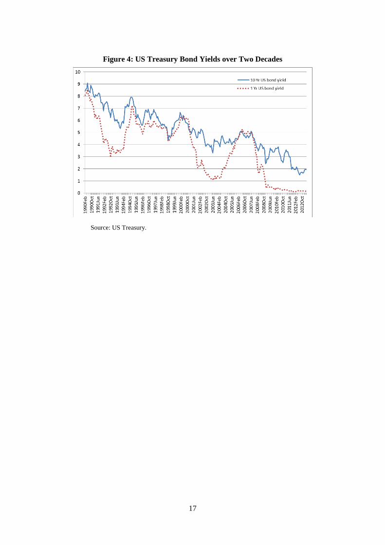
Figure 4: US Treasury Bond Yields over Two Decades

Source: US Treasury.

17

Figure 5: US, European and Japanese Government Bond Yields Since 2000

Source: US Treasury.

Source: European Central Bank.

Source: European Central Bank, Reuters.

18

Figure 6: Central Bank Assets, US$ trillions

Sources: EU, ECB; United States, Japan: St. Louis Federal Reserve Database; China, National Bureau of Statistics.

Figure 7: Nominal Exchange Rate Indices vs the US$

Source: IMF IFS and Eurostat.

19

Table 1: Relative Economic Sizes of China and the Other Large Regions, ca 2011:

% of world China US EU(26) Japan GDP 11 22 26 9 Consumption, C 8 27 26 9 Investment, I 20 15 22 8 Government spending, G 7 20 30 10 Exports, X 17 17 25 7 Imports, M 15 21 23 8 Total domestic saving, SD 19 13 20 9 Sources: National accounts data supply most of the elements though adjustments have been required to ensure that current accounts sum to zero globally, as do capital/financial accounts. The IMF-IFS database is the major source but there is frequent resort to national statistical databases.

Table 2: Regional Economic Structure, 2011:

% of GDP US EU(26) Japan China Australia RoW C 0.712 0.580 0.605 0.450 0.536 0.550 I 0.155 0.191 0.200 0.410 0.275 0.240 G 0.171 0.217 0.204 0.114 0.177 0.199 X 0.139 0.175 0.151 0.285 0.217 0.200 M 0.177 0.163 0.161 0.259 0.204 0.189 Indirect tax rev, TI 0.144 0.235 0.047 0.125 0.070 0.130 Direct tax rev, TD 0.017 0.015 0.124 0.035 0.093 0.061 Total tax rev, T 0.161 0.250 0.171 0.160 0.163 0.191 Private saving, SP 0.127 0.169 0.224 0.390 0.301 0.259 Govt saving, SG -0.010 0.034 -0.034 0.046 -0.013 -0.008 Total saving, SD 0.155 0.191 0.200 0.410 0.275 0.240 Monetary base, MB 0.133 0.114 0.220 0.411 0.134 0.250 Capital stock, K 3.317 3.414 4.239 2.740 4.027 2.000 Sources: National accounts data supply most of the elements though adjustments have been required to ensure that current accounts sum to zero globally, as do capital/financial accounts. The IMF-IFS database is the major source but there is frequent resort to national statistical databases.

Table 3: Shares of Consumption by Region of Origin, 2011a

% of row consn expenditure

US EU(26) Japan China Australia RoW

US 65.9 10.3 2.3 6.1 0.5 14.9 EU(26) 12.0 43.9 2.9 11.2 0.6 29.4 Japan 4.7 5.1 69.1 6.5 2.3 12.3 China 10.4 18.2 11.2 17.6 4.5 38.1 Australia 8.1 12.8 3.8 9.2 53.7 12.5 Rest of world 14.4 22.0 3.9 10.6 1.0 48.1 a These shares sum to 100 horizontally. They are based on the 2011 matrix of trade flows combined with consumption expenditure data in each region. The resulting matrix is inconsistent as between data sources and so a RAS algorithm is used to force consistency of bilateral elements with national accounts data. Sources: Implied trade flows are for 2011, drawn from the World Trade Organisation database.

20

Table 4: Shares of Total Domestic Saving Directed to Investment in Each Region, 2011a

% of row total saving US EU(26) Japan China Australia RoW

USb 68.0 13.3 6.4 6.4 1.5 4.4 EU(26)c 12.9 80.1 2.3 2.3 0.9 1.5 Japand 14.0 3.3 72.2 6.2 0.7 3.6 Chinac 9.2 0.6 0.9 81.1 0.1 8.0 Australiae 13.0 4.8 2.3 2.1 77.3 0.4 Rest of world 3.4 3.9 2.6 2.8 0.1 87.2 a These shares sum to 100 horizontally. They are based on 2011 investment flows. The original flow matrix is inconsistent with data on saving and investment from national accounts and so a RAS algorithm is used to ensure that row and column sums are consistent with other data. The row sums of the flow matrix are total saving by region and the column sums are total investment by region. These sums are sourced from the IMF-IFS database and the World Bank database. b USA: values are based on official statistics, BEA. c EU and China: indirect information from USA, Australian and Japanese statistics. d Japan: estimated based on FDI data, assuming investment outflow=FDI*1.6. The ratio 1.6 is that of USA reported inward investment from Japan divided by Japanese reported outward FDI to the USA. e Australia: Australian Bureau of Statistics "International Investment Position, Australia: Supplementary Statistics, 2011". f ROW is a residual. Its saving is inferred from national accounts estimates and its investment abroad is determined to balance the matrix of financial flows.

21

Table 5: Parameters

US EU(26) Japan China Australia RoW Production sharesa Labour, βL 0.18 0.18 0.18 0.26 0.18 0.24 Skill, βS 0.47 0.47 0.47 0.24 0.47 0.21 Capital, βK 0.35 0.35 0.35 0.50 0.35 0.55 Income tax ratesb tL= tS= tK 0.02 0.02 0.13 0.04 0.10 0.07 Indirect tax ratesc tC 0.20 0.40 0.05 0.20 0.10 0.15 tM 0.15 0.43 0.11 0.19 0.11 0.31 tX 0.00 0.00 0.00 0.00 0.00 0.00 Money parametersd Reserve ratio, ρ 0.05 0.05 0.05 0.15 0.05 0.10 Cash ratio, μ 0.08 0.10 0.17 0.21 0.10 0.20 Elasticities c to r, εCR 0.10 0.10 0.10 0.10 0.10 0.10 c to YD, εCY 0.94 1.03 0.82 0.93 1.25 0.88 cij/cik to PC

ij/PCik, σi 2.00 2.00 2.00 2.00 2.00 2.00

Saving iSij to ri/rj, σI

i 15.0 15.0 15.0 15.0 15.0 5.0 Investment, Ii to rC

i/ri, εIi 1.00 1.00 1.00 1.00 1.00 1.00

Premium to G/T, ϕi 0.20 0.20 0.20 0.20 0.20 0.20 mD to y, εMY 1.00 1.00 1.00 1.00 1.00 1.00 mD to (r+πe), εMR 0.60 0.60 0.60 0.60 0.60 0.60 a Production shares are based on demographic and occupational data from Tyers and Bain (2006), as well as estimates of factor incomes and capital stocks from the GTAP Database. b These income tax rates are lower than observed because direct transfers and sovereign debt service are deducted from income tax revenue so that observed fiscal balances are consistent with T-G, where G includes only expenditure on goods and services. c Although export taxes appear in the modelling, no values are applied since such taxes are usually very indirect. To infer the rates for other indirect taxes, approximate rates are initially chosen for the consumption tax rate and the import tax rate is then determined for consistency with the data on indirect tax revenue. In regions where other indirect taxes are major contributors to revenue, this tends to inflate the values of tC and tM. d The money parameters are crude characterisations, made on the assumption that the EU behaves as if it had a single central bank to cover all 26 members. Money demand parameters stem from a survey of estimates used in other models (including McKibbin and Wilcoxen 1995, Knell and Stix, 2003 and Teles and Zhou 2005). e Consumption elasticities are consistent with a variety of estimates in use in other models, both of marginal propensities and elasticities (including McKibbin and Wilcoxen 1995 and Jin 2011).

22

Table 6: Exogenous Variables for Experimentation

Policy Instrument Tax rates Labour income tax tL Capital income tax tK Consumption tax (GST) tC Import tariff tM Export tax tX Fiscal policy Government spending, US$ trillion G fiscal surplus, US$ trillion SG Monetary policy Monetary base, US$ trillion MB Reserve to deposit ratio ρ Expectations over future values Consumer price inflation rate πCe GDP price inflation rate πYe Real exchange rate appreciation ˆee Nominal disposable income YD

e Rate of return on installed capital rC

e Productivity TFP AY Saving Consumption preference shifter AC

Table 7: Closure Choices and Policy Regimes

In each case, holding fixed or exogenous one of:

Labour market Nominal wage W Labour use L Government Nominal expenditure G Fiscal surplus SG=T-G Monetary target Monetary base MB Consumer price level PC GDP price level PY Producer price level PP Exchange rate E

23

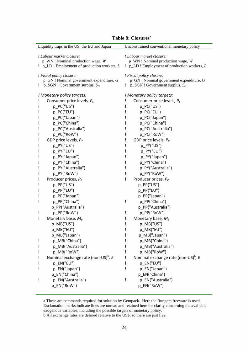
Table 8: Closuresa

Liquidity traps in the US, the EU and Japan Unconstrained conventional monetary policy ! Labour market closure: ! Labour market closure: p_WN ! Nominal production wage, W p_WN ! Nominal production wage, W ! p_LD ! Employment of production workers, L ! p_LD ! Employment of production workers, L ! Fiscal policy closure: ! Fiscal policy closure: p_GN ! Nominal government expenditure, G p_GN ! Nominal government expenditure, G ! p_SGN ! Government surplus, SG ! p_SGN ! Government surplus, SG ! Monetary policy targets: ! Monetary policy targets: ! Consumer price levels, PC ! Consumer price levels, PC ! p_PC("US") ! p_PC("US") ! p_PC("EU") ! p_PC("EU") ! p_PC("Japan") ! p_PC("Japan") ! p_PC("China") ! p_PC("China") ! p_PC("Australia") ! p_PC("Australia") ! p_PC("RoW") ! p_PC("RoW") ! GDP price levels, PY ! GDP price levels, PY ! p_PY("US") ! p_PY("US") ! p_PY("EU") ! p_PY("EU") ! p_PY("Japan") ! p_PY("Japan") ! p_PY("China") ! p_PY("China") ! p_PY("Australia") ! p_PY("Australia") ! p_PY("RoW") ! p_PY("RoW") ! Producer prices, PP ! Producer prices, PP ! p_PP("US") p_PP("US") ! p_PP("EU") p_PP("EU") ! p_PP("Japan") p_PP("Japan") ! p_PP("China") ! p_PP("China") p_PP("Australia") p_PP("Australia") ! p_PP("RoW") ! p_PP("RoW") ! Monetary base, MB ! Monetary base, MB p_MB("US") ! p_MB("US") p_MB("EU") ! p_MB("EU") p_MB("Japan") ! p_MB("Japan") ! p_MB("China") ! p_MB("China") ! p_MB("Australia") ! p_MB("Australia") ! p_MB("RoW") ! p_MB("RoW") ! Nominal exchange rate (non-US)b, E ! Nominal exchange rate (non-US)b, E ! p_EN("EU") ! p_EN("EU") ! p_EN("Japan") ! p_EN("Japan") p_EN("China") p_EN("China") ! p_EN("Australia") ! p_EN("Australia") p_EN("RoW") p_EN("RoW")

a These are commands required for solution by Gempack. Here the Rungem freeware is used. Exclamation marks indicate lines are unread and retained here for clarity concerning the available exogenous variables, including the possible targets of monetary policy. b All exchange rates are defined relative to the US$, so there are just five.

24

Table 9: Pessimistic Expectation Shocks in the US, EU and Japana

Shocks (%) to Exogenous Expectational Variables Consumer price inflation, which affects consumption, via 1 π= + CeINFE Shock p_INFE("US") = -5; Shock p_INFE("EU") = -5; Shock p_INFE("Japan") = -5; GDP price inflation, which affects money demand, via 1 π= + YeRNFE Shock p_RNFE("US") = -5; Shock p_RNFE("EU") = -5; Shock p_RNFE("Japan") = -5; Expected future nominal disposable income, = DeYDNE Y Shock p_YDNE(“US”) = -10; Shock p_YDNE(“EU”) = -10; Shock p_YDNE(“Japan”) = -10; Expected future net rate of return on installed capital, factor on = e

CRCE r Shock p_RC_EXP("US") = -2; Shock p_RC_EXP("EU") = -2; Shock p_RC_EXP("Japan") = -2;

a These are commands required for solution by Gempack. Here the Rungem freeware is used.

25

Table 10: Pessimistic Expectations in the US, EU and Japan: Simulation Results

% change US EU(26) Japan China Australia RoW US, EU, Japan liquidity trap (MB fixed) Monetary base, MB 0.0b 0.0b 0.0b -1.1 0.2 -1.9 Prices and exchange rates Consumer price level, PC -1.9 -2.3 -2.5 -1.1 -0.2 -1.1 Producer price level, PP -2.4 -2.1 -2.5 -0.7 0.0b -0.9 GDP price level, PY -2.8 -2.8 -2.6 -0.6 0.0 -0.8 Nominal exch rate v US, E 0.0 1.3 1.4 0.0b -0.6 0.0b Real exch rate v US, e 0.0 1.3 1.6 2.3 2.3 2.1 Interest rates Real bond yield, r -0.8 -0.7 -0.4 0.4 -0.3 1.3 Nominal bond yield, r+ πYe -5.7 -5.7 -5.4 0.4 -0.3 1.3 Balance of payments Change in CA, %GDP 1.1 0.3 0.3 -1.0 -0.6 -0.8 Real volumes Real consumption, c -4.1 -3.4 -2.8 1.0 0.6 0.8 Real investment, I/PP 0.6 0.4 0.9 1.2 1.5 0.5 Labour use, L -2.9 -2.6 -3.1 -1.0 0.0c -1.2 Real GDP, y=Y/PY -0.5 -0.5 -0.6 -0.3 0.0c -0.3 Purchasing power of income at consumer prices Welfare, Y/PC -1.5 -1.0 -0.7 0.2 0.3 0.0 Effective monetary policy in US, EU and Japan, targeting producer price levels Monetary base, MB 10.7 10.2 11.8 16.5 7.1 12.7 Prices and exchange rates Consumer price level, PC 1.4 -0.5 2.1 3.8 -5.0 3.6 Producer price level, PP 0.0b 0.0b 0.0b 6.3 0.0b 4.1 GDP price level, PY -0.7 -0.8 -0.3 6.0 0.8 3.8 Nominal exch rate v US, E 0.0 4.4 -2.3 0.0b 15.1 0.0b Real exch rate v US, e 0.0 4.3 -1.9 6.8 16.9 4.6 Interest rates Real bond yield, r -14.9 -14.1 -16.0 -12.7 -10.5 -12.3 Nominal bond yield, r+ πYe -19.2 -18.4 -20.2 -12.7 -10.5 -12.3 Balance of payments Change in CA, %GDP 2.2 -0.1 3.0 -2.5 -9.0 -0.9 Real volumes Real consumption, c -5.9 -2.9 -6.0 2.3 15.1 -0.3 Real investment, I/PP 2.4 7.2 -4.8 12.6 13.8 12.8 Labour use, L 0.0c 0.0c 0.0c 8.7 0.0c 5.4 Real GDP, y=Y/PY 0.0c 0.0c 0.0c 2.2 0.0c 1.2 Purchasing power of income at consumer prices Welfare, Y/PC -2.1 -0.2 -2.3 4.5 6.1 1.5 a These results are generated by the Gempack-Rungem software from the closures and shocks listed in Table 8. b These are targets of monetary policy. c These are the direct consequences of targeting producer price levels.

26

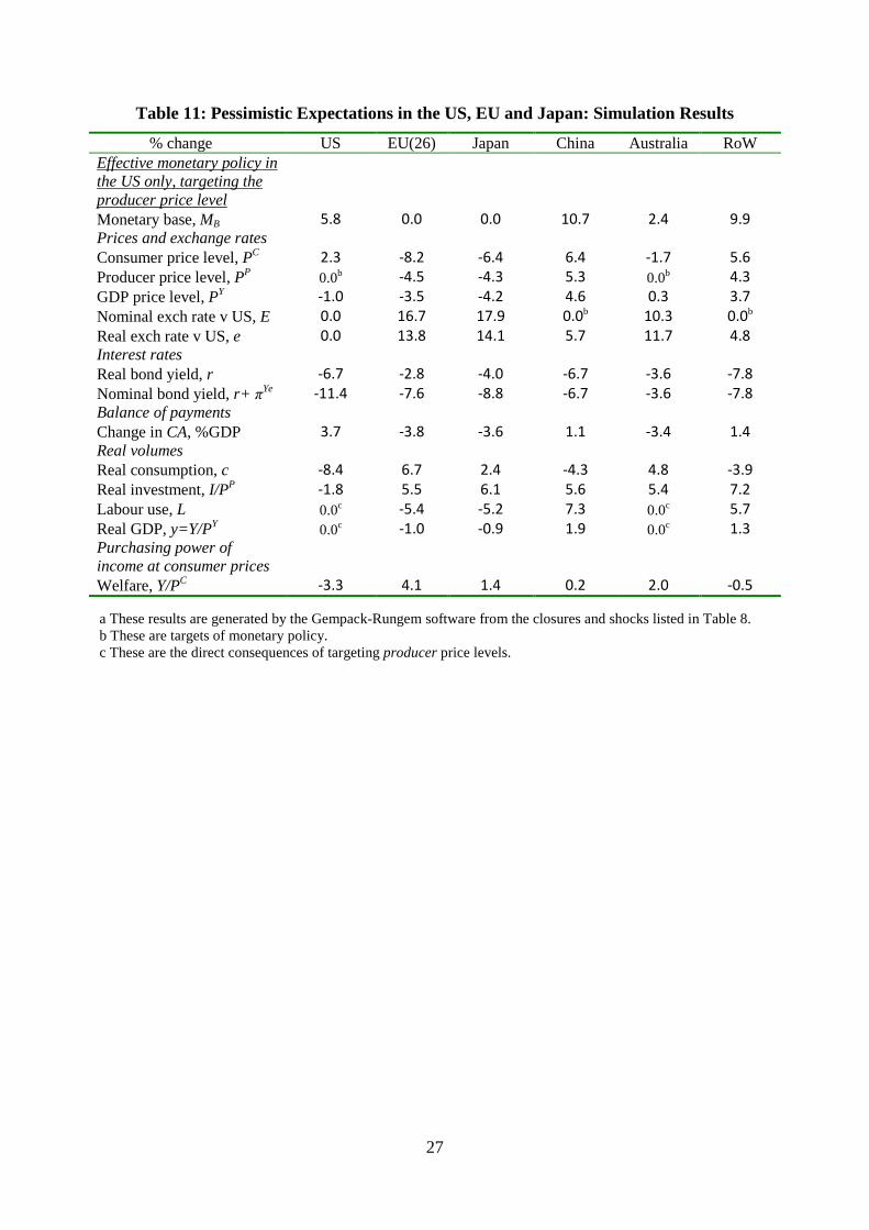
Table 11: Pessimistic Expectations in the US, EU and Japan: Simulation Results

% change US EU(26) Japan China Australia RoW Effective monetary policy in the US only, targeting the producer price level Monetary base, MB 5.8 0.0 0.0 10.7 2.4 9.9 Prices and exchange rates Consumer price level, PC 2.3 -8.2 -6.4 6.4 -1.7 5.6 Producer price level, PP 0.0b -4.5 -4.3 5.3 0.0b 4.3 GDP price level, PY -1.0 -3.5 -4.2 4.6 0.3 3.7 Nominal exch rate v US, E 0.0 16.7 17.9 0.0b 10.3 0.0b Real exch rate v US, e 0.0 13.8 14.1 5.7 11.7 4.8 Interest rates Real bond yield, r -6.7 -2.8 -4.0 -6.7 -3.6 -7.8 Nominal bond yield, r+ πYe -11.4 -7.6 -8.8 -6.7 -3.6 -7.8 Balance of payments Change in CA, %GDP 3.7 -3.8 -3.6 1.1 -3.4 1.4 Real volumes Real consumption, c -8.4 6.7 2.4 -4.3 4.8 -3.9 Real investment, I/PP -1.8 5.5 6.1 5.6 5.4 7.2 Labour use, L 0.0c -5.4 -5.2 7.3 0.0c 5.7 Real GDP, y=Y/PY 0.0c -1.0 -0.9 1.9 0.0c 1.3 Purchasing power of income at consumer prices Welfare, Y/PC -3.3 4.1 1.4 0.2 2.0 -0.5 a These results are generated by the Gempack-Rungem software from the closures and shocks listed in Table 8. b These are targets of monetary policy. c These are the direct consequences of targeting producer price levels.

27

Appendix 1: Model Analytics – The Conventional Components

Key financial relationships are given in the main text. This appendix lists the more standard

details of the model’s specification.

Output is assumed to be Cobb-Douglas in the three primary factors, so that, for regions i, local

output and the marginal product of capital are:

(A1) L S K S Ki i i i i L1Y K K Y K L S Ki

i i i i i i i i i i i i i i ii

yy A L S K , MP A S K L , 1 iK

β β β β β ββ β β β β− = = = + + = " .

The real volume of output, y, is distinguished from nominal GDP, Y = PYy, where PY is the

GDP price level (deflator). The real production wages of unskilled and skilled workers depend

conventionally on the corresponding marginal products.

(A2) S

L S Si i i ii i i iP P

i i i i

W y W yw , wP L P S

β β= = = =

Here the upper case wages are nominal and the lower case real and PP is the producer price

level.

Both direct and indirect tax revenues, TD and TI, play key roles in the formulation. GDP at

factor cost (or producer prices), YFC, is the total of direct payments to the collective household

in return for the use of its factors. Region i’s nominal GDP is then

(A3) FC FCI D P

i i i i i i iY Y T , Y C T S= + = + +

This is the standard disposal identity for GDP, or the collective household budget, where C is

the total value of final consumption expenditure, including indirect taxes paid, and SP is private

saving. The GDP price, PY, and the producer price, PP, would be the same were it not for

indirect taxes. In their presence we have:

(A4) Y P Ii i i i i iY P y P y T= = + , so that

IY P i

i ii

TP Py

= + .

Direct tax

Constant marginal direct tax rates, tW and tK, apply to all labour and capital income. The

corresponding “powers” of these rates are ( )L L1 tτ = + and ( )K K1 tτ = + and total direct tax

revenue is:

28

(A5) ( )D L S K P Ki i i k i i i i i iT t W L W S t P MP K= + + .

Indirect tax revenue, TI, depends on consumption and trade and so it will emerge later.

Consumption

Aggregate consumption expenditure, C, is a nominal sum but real consumption behaviour is

motivated by real incomes and the real interest rate. Real consumption, (lower case) c,

depends negatively on the real after-tax return on savings (the home bond yield, r) and

positively on both current and expected future real disposable income:

(A6) ee e

τ π

− = = +

CYCR CY ii iD DeCi i i i

i iC K C C Cei i i i i

C r Y Yc AP P P 1

,

where the expected inflation rate of the consumer price level is π Ce . To capture the home

household’s substitution between home and foreign products, real aggregate consumption in

region i is a CES composite of region i’s consumption of products from all regions:

(A7) i

i

1

i ij ijj

c cθ

θa−

− = ∑

The home household then chooses its mix of consumed products to minimise consumption

expenditure in a way that accounts for home indirect tax rates, foreign export taxes and

differing foreign product prices and exchange rates:

(A8) jC P C C M X Pi i i i i ii i i j ij j

j i

EC P c P c c P

Eτ τ τ τ= = +∑ ,

where C Mi i,τ τ and X

jτ are, respectively, the powers of region i’s consumption and import taxes

and the region of origin, j’s export tax. Ei is region i’s nominal exchange rate, measured as

US$ per unit of home currency.15

Optimum consumption is consistent with an elasticity of substitution between home and

foreign products of ( )i i1 / 1σ θ= + . The Marshallian demands are then:

(A9) ( )

, ,ii

i i

C M PP Ci i j j ii i i i

ii ii ij ijC C C Ci i i i

P E EC P Cc c i jP P P P

σσσ σ

τ ττa a

−− = = ≠

.

15 US currency is the numeraire in the model.

29

Given these consumption volumes, the composite price of all consumption, or the consumer

price level, emerges from the substitution of (A7) and (A9) in (A8) as:

(A10) ( )1

1 11

i ii

i i

Pj jC C P M

i i ii i i ijj i i

P EP P

E

σ σσσ στ a τ a

− −−

≠

= +

∑

The global product balance

Each region’s product is differentiated from the others and so global product balance stems

from a version of the expenditure identity in real volume terms:

(A11) i ii jiP

ji

I Gy cP+

= +∑ ,

where the final term is the sum of real consumption and real exports. Neither investors nor the

government pay indirect taxes on their expenditure and so the price they face for the home

product is the producer price, PP. This equation solves indirectly for the producer prices.

Private saving

Households receive income amounting to GDP at factor cost, YFC. Their disposable nominal

income is this sum less direct tax (6), and private saving is what remains after consumption

expenditure (9) is further deducted.

(A12) ,D P D P Di i i i i i iY P y T S Y C= − = −

Indirect tax revenue

This includes revenue from consumption, import and export taxes:

(A13) jC C P M X Pi i i ii i j ij j

j i

ET t P c c P

Eτ τ

= +

∑ ,

(A14) , jM M X Pi i i i j ij j

j i i

ET t M M c P

Eτ

≠

= =∑ ,

(A15) ,X X Pi i i i ji i

jT t X X c P= =∑ ,

(A16) I C M X D Ii i i i i i iT T T T , T T T= + + = + .

30

Government and total domestic saving

This is government revenue less government expenditure, both measured net of direct transfers.

To simplify the demand side, spending by the government is assumed to be directed only at

home goods.16 It pays no taxes and so faces the home producer price PP. Total domestic

saving is then the sum of private and government savings in the home economy, in home

currency.

(A17) D P G P D Ii i i iS S S S T T G= + = + + − .

Balance of payments

The sum of net inflows of payments on the current account and net inflows on the capital and

financial accounts, measured in a single (home) currency is zero:

(A18) ( )jS D S Di i ji j ij i

j i j ii

EX M i S i S 0, i "US"

E≠ ≠

− + − = " ≠

∑ ∑

Balance in the US is implied by balance in all the other regions. These equations determine the

nominal exchange rates and, since these are defined relative to the US$, that for the US is

always unity ( )USE 1= .

Real exchange rate

Each region has a real exchange rate relative to the US that is the rate of exchange between

regional product bundles. With the regions specified as single product economies this measure

parallels the terms of trade. Both real and nominal exchange rates are expressed according to

the financial convention, so that an appreciation is a rise in value.

(A19) Y Y

i ii i YY

USUS

i

P Pe EPP

E

= =

.

16 In the model database, direct transfers are netted from direct tax revenue, so that T-G is the true fiscal surplus.

31

Editor, UWA Economics Discussion Papers: Ernst Juerg Weber Business School – Economics University of Western Australia 35 Sterling Hwy Crawley WA 6009 Australia Email: ecoadmin@biz.uwa.edu.au The Economics Discussion Papers are available at: 1980 – 2002: http://ecompapers.biz.uwa.edu.au/paper/PDF%20of%20Discussion%20Papers/ Since 2001: http://ideas.repec.org/s/uwa/wpaper1.html Since 2004: http://www.business.uwa.edu.au/school/disciplines/economics

ECONOMICS DISCUSSION PAPERS 2012

DP NUMBER AUTHORS TITLE

12.01 Clements, K.W., Gao, G., and Simpson, T.

DISPARITIES IN INCOMES AND PRICES INTERNATIONALLY

12.02 Tyers, R. THE RISE AND ROBUSTNESS OF ECONOMIC FREEDOM IN CHINA

12.03 Golley, J. and Tyers, R. DEMOGRAPHIC DIVIDENDS, DEPENDENCIES AND ECONOMIC GROWTH IN CHINA AND INDIA

12.04 Tyers, R. LOOKING INWARD FOR GROWTH

12.05 Knight, K. and McLure, M. THE ELUSIVE ARTHUR PIGOU

12.06 McLure, M. ONE HUNDRED YEARS FROM TODAY: A. C. PIGOU’S WEALTH AND WELFARE

12.07 Khuu, A. and Weber, E.J. HOW AUSTRALIAN FARMERS DEAL WITH RISK

12.08 Chen, M. and Clements, K.W. PATTERNS IN WORLD METALS PRICES

12.09 Clements, K.W. UWA ECONOMICS HONOURS

12.10 Golley, J. and Tyers, R. CHINA’S GENDER IMBALANCE AND ITS ECONOMIC PERFORMANCE

12.11 Weber, E.J. AUSTRALIAN FISCAL POLICY IN THE AFTERMATH OF THE GLOBAL FINANCIAL CRISIS

12.12 Hartley, P.R. and Medlock III, K.B. CHANGES IN THE OPERATIONAL EFFICIENCY OF NATIONAL OIL COMPANIES

12.13 Li, L. HOW MUCH ARE RESOURCE PROJECTS WORTH? A CAPITAL MARKET PERSPECTIVE

12.14 Chen, A. and Groenewold, N. THE REGIONAL ECONOMIC EFFECTS OF A REDUCTION IN CARBON EMISSIONS AND AN EVALUATION OF OFFSETTING POLICIES IN CHINA

12.15 Collins, J., Baer, B. and Weber, E.J. SEXUAL SELECTION, CONSPICUOUS CONSUMPTION AND ECONOMIC GROWTH

32

ECONOMICS DISCUSSION PAPERS 2012

DP NUMBER AUTHORS TITLE

12.16 Wu, Y. TRENDS AND PROSPECTS IN CHINA’S R&D SECTOR

12.17 Cheong, T.S. and Wu, Y. INTRA-PROVINCIAL INEQUALITY IN CHINA: AN ANALYSIS OF COUNTY-LEVEL DATA

12.18 Cheong, T.S. THE PATTERNS OF REGIONAL INEQUALITY IN CHINA

12.19 Wu, Y. ELECTRICITY MARKET INTEGRATION: GLOBAL TRENDS AND IMPLICATIONS FOR THE EAS REGION

12.20 Knight, K. EXEGESIS OF DIGITAL TEXT FROM THE HISTORY OF ECONOMIC THOUGHT: A COMPARATIVE EXPLORATORY TEST

12.21 Chatterjee, I. COSTLY REPORTING, EX-POST MONITORING, AND COMMERCIAL PIRACY: A GAME THEORETIC ANALYSIS

12.22 Pen, S.E. QUALITY-CONSTANT ILLICIT DRUG PRICES

12.23 Cheong, T.S. and Wu, Y. REGIONAL DISPARITY, TRANSITIONAL DYNAMICS AND CONVERGENCE IN CHINA

12.24 Ezzati, P. FINANCIAL MARKETS INTEGRATION OF IRAN WITHIN THE MIDDLE EAST AND WITH THE REST OF THE WORLD

12.25 Kwan, F., Wu, Y. and Zhuo, S. RE-EXAMINATION OF THE SURPLUS AGRICULTURAL LABOUR IN CHINA

12.26 Wu, Y. R&D BEHAVIOUR IN CHINESE FIRMS

12.27 Tang, S.H.K. and Yung, L.C.W. MAIDS OR MENTORS? THE EFFECTS OF LIVE-IN FOREIGN DOMESTIC WORKERS ON SCHOOL CHILDREN’S EDUCATIONAL ACHIEVEMENT IN HONG KONG

12.28 Groenewold, N. AUSTRALIA AND THE GFC: SAVED BY ASTUTE FISCAL POLICY?

33

ECONOMICS DISCUSSION PAPERS 2013

DP NUMBER AUTHORS TITLE

13.01 Chen, M., Clements, K.W. and Gao, G.

THREE FACTS ABOUT WORLD METAL PRICES

13.02 Collins, J. and Richards, O. EVOLUTION, FERTILITY AND THE AGEING POPULATION

13.03 Clements, K., Genberg, H., Harberger, A., Lothian, J., Mundell, R., Sonnenschein, H. and Tolley, G.

LARRY SJAASTAD, 1934-2012

13.04 Robitaille, M.C. and Chatterjee, I. MOTHERS-IN-LAW AND SON PREFERENCE IN INDIA

13.05 Clements, K.W. and Izan, I.H.Y. REPORT ON THE 25TH PHD CONFERENCE IN ECONOMICS AND BUSINESS

13.06 Walker, A. and Tyers, R. QUANTIFYING AUSTRALIA’S “THREE SPEED” BOOM

13.07 Yu, F. and Wu, Y. PATENT EXAMINATION AND DISGUISED PROTECTION

13.08 Yu, F. and Wu, Y. PATENT CITATIONS AND KNOWLEDGE SPILLOVERS: AN ANALYSIS OF CHINESE PATENTS REGISTER IN THE US

13.09 Chatterjee, I. and Saha, B. BARGAINING DELEGATION IN MONOPOLY

13.10 Cheong, T.S. and Wu, Y. GLOBALIZATION AND REGIONAL INEQUALITY IN CHINA

13.11 Cheong, T.S. and Wu, Y. INEQUALITY AND CRIME RATES IN CHINA

13.12 Robertson, P.E. and Ye, L. ON THE EXISTENCE OF A MIDDLE INCOME TRAP

13.13 Robertson, P.E. THE GLOBAL IMPACT OF CHINA’S GROWTH

13.14 Hanaki, N., Jacquemet, N., Luchini, S., and Zylbersztejn, A.

BOUNDED RATIONALITY AND STRATEGIC UNCERTAINTY IN A SIMPLE DOMINANCE SOLVABLE GAME

13.15 Okatch, Z., Siddique, A. and Rammohan, A.

DETERMINANTS OF INCOME INEQUALITY IN BOTSWANA

13.16 Clements, K.W. and Gao, G. A MULTI-MARKET APPROACH TO MEASURING THE CYCLE

13.17 Chatterjee, I. and Ray, R. THE ROLE OF INSTITUTIONS IN THE INCIDENCE OF CRIME AND CORRUPTION

13.18 Fu, D. and Wu, Y. EXPORT SURVIVAL PATTERN AND DETERMINANTS OF CHINESE MANUFACTURING FIRMS

13.19 Shi, X., Wu, Y. and Zhao, D. KNOWLEDGE INTENSIVE BUSINESS SERVICES AND THEIR IMPACT ON INNOVATION IN CHINA

13.20 Tyers, R., Zhang, Y. and Cheong, T.S.

CHINA’S SAVING AND GLOBAL ECONOMIC PERFORMANCE

13.21 Collins, J., Baer, B. and Weber, E.J. POPULATION, TECHNOLOGICAL PROGRESS AND THE EVOLUTION OF INNOVATIVE POTENTIAL

13.22 Hartley, P.R. THE FUTURE OF LONG-TERM LNG CONTRACTS

13.23 Tyers, R. A SIMPLE MODEL TO STUDY GLOBAL MACROECONOMIC INTERDEPENDENCE

34

ECONOMICS DISCUSSION PAPERS 2013

DP NUMBER AUTHORS TITLE

13.24 McLure, M. REFLECTIONS ON THE QUANTITY THEORY: PIGOU IN 1917 AND PARETO IN 1920-21

13.25 Chen, A. and Groenewold, N. REGIONAL EFFECTS OF AN EMISSIONS-REDUCTION POLICY IN CHINA: THE IMPORTANCE OF THE GOVERNMENT FINANCING METHOD

13.26 Siddique, M.A.B. TRADE RELATIONS BETWEEN AUSTRALIA AND THAILAND: 1990 TO 2011

13.27 Li, B. and Zhang, J. GOVERNMENT DEBT IN AN INTERGENERATIONAL MODEL OF ECONOMIC GROWTH, ENDOGENOUS FERTILITY, AND ELASTIC LABOR WITH AN APPLICATION TO JAPAN

13.28 Robitaille, M. and Chatterjee, I. SEX-SELECTIVE ABORTIONS AND INFANT MORTALITY IN INDIA: THE ROLE OF PARENTS’ STATED SON PREFERENCE

13.29 Ezzati, P. ANALYSIS OF VOLATILITY SPILLOVER EFFECTS: TWO-STAGE PROCEDURE BASED ON A MODIFIED GARCH-M

13.30 Robertson, P. E. DOES A FREE MARKET ECONOMY MAKE AUSTRALIA MORE OR LESS SECURE IN A GLOBALISED WORLD?

13.31 Das, S., Ghate, C. and Robertson, P. E.

REMOTENESS AND UNBALANCED GROWTH: UNDERSTANDING DIVERGENCE ACROSS INDIAN DISTRICTS

13.32 Robertson, P.E. and Sin, A. MEASURING HARD POWER: CHINA’S ECONOMIC GROWTH AND MILITARY CAPACITY

13.33 Wu, Y. TRENDS AND PROSPECTS FOR THE RENEWABLE ENERGY SECTOR IN THE EAS REGION

13.34 Yang, S., Zhao, D., Wu, Y. and Fan, J.

REGIONAL VARIATION IN CARBON EMISSION AND ITS DRIVING FORCES IN CHINA: AN INDEX DECOMPOSITION ANALYSIS

35

ECONOMICS DISCUSSION PAPERS 2014

DP NUMBER AUTHORS TITLE

14.01 Boediono, Vice President of the Republic of Indonesia

THE CHALLENGES OF POLICY MAKING IN A YOUNG DEMOCRACY: THE CASE OF INDONESIA (52ND SHANN MEMORIAL LECTURE, 2013)

14.02 Metaxas, P.E. and Weber, E.J. AN AUSTRALIAN CONTRIBUTION TO INTERNATIONAL TRADE THEORY: THE DEPENDENT ECONOMY MODEL

14.03 Fan, J., Zhao, D., Wu, Y. and Wei, J. CARBON PRICING AND ELECTRICITY MARKET REFORMS IN CHINA

14.04 McLure, M. A.C. PIGOU’S MEMBERSHIP OF THE ‘CHAMBERLAIN-BRADBURY’ COMMITTEE. PART I: THE HISTORICAL CONTEXT

14.05 McLure, M. A.C. PIGOU’S MEMBERSHIP OF THE ‘CHAMBERLAIN-BRADBURY’ COMMITTEE. PART II: ‘TRANSITIONAL’ AND ‘ONGOING’ ISSUES

14.06 King, J.E. and McLure, M. HISTORY OF THE CONCEPT OF VALUE

14.07 Williams, A. A GLOBAL INDEX OF INFORMATION AND POLITICAL TRANSPARENCY

14.08 Knight, K. A.C. PIGOU’S THE THEORY OF UNEMPLOYMENT AND ITS CORRIGENDA: THE LETTERS OF MAURICE ALLEN, ARTHUR L. BOWLEY, RICHARD KAHN AND DENNIS ROBERTSON

14.09

Cheong, T.S. and Wu, Y. THE IMPACTS OF STRUCTURAL RANSFORMATION AND INDUSTRIAL UPGRADING ON REGIONAL INEQUALITY IN CHINA

14.10 Chowdhury, M.H., Dewan, M.N.A., Quaddus, M., Naude, M. and Siddique, A.

GENDER EQUALITY AND SUSTAINABLE DEVELOPMENT WITH A FOCUS ON THE COASTAL FISHING COMMUNITY OF BANGLADESH

14.11 Bon, J. UWA DISCUSSION PAPERS IN ECONOMICS: THE FIRST 750

14.12 Finlay, K. and Magnusson, L.M. BOOTSTRAP METHODS FOR INFERENCE WITH CLUSTER-SAMPLE IV MODELS

14.13 Chen, A. and Groenewold, N. THE EFFECTS OF MACROECONOMIC SHOCKS ON THE DISTRIBUTION OF PROVINCIAL OUTPUT IN CHINA: ESTIMATES FROM A RESTRICTED VAR MODEL

14.14 Hartley, P.R. and Medlock III, K.B. THE VALLEY OF DEATH FOR NEW ENERGY TECHNOLOGIES

14.15 Hartley, P.R., Medlock III, K.B., Temzelides, T. and Zhang, X.

LOCAL EMPLOYMENT IMPACT FROM COMPETING ENERGY SOURCES: SHALE GAS VERSUS WIND GENERATION IN TEXAS

14.16 Tyers, R. and Zhang, Y. SHORT RUN EFFECTS OF THE ECONOMIC REFORM AGENDA

14.17 Clements, K.W., Si, J. and Simpson, T. UNDERSTANDING NEW RESOURCE PROJECTS

14.18 Tyers, R. SERVICE OLIGOPOLIES AND AUSTRALIA’S ECONOMY-WIDE PERFORMANCE

36

ECONOMICS DISCUSSION PAPERS 2014

DP NUMBER AUTHORS TITLE

14.19 Tyers, R. and Zhang, Y. REAL EXCHANGE RATE DETERMINATION AND THE CHINA PUZZLE

14.20 Ingram, S.R. COMMODITY PRICE CHANGES ARE CONCENTRATED AT THE END OF THE CYCLE

14.21 Cheong, T.S. and Wu, Y. CHINA'S INDUSTRIAL OUTPUT: A COUNTY-LEVEL STUDY USING A NEW FRAMEWORK OF DISTRIBUTION DYNAMICS ANALYSIS

14.22 Siddique, M.A.B., Wibowo, H. and Wu, Y.

FISCAL DECENTRALISATION AND INEQUALITY IN INDONESIA: 1999-2008

14.23 Tyers, R. ASYMMETRY IN BOOM-BUST SHOCKS: AUSTRALIAN PERFORMANCE WITH OLIGOPOLY

14.24 Arora, V., Tyers, R. and Zhang, Y. RECONSTRUCTING THE SAVINGS GLUT: THE GLOBAL IMPLICATIONS OF ASIAN EXCESS SAVING

14.25 Tyers, R. INTERNATIONAL EFFECTS OF CHINA’S RISE AND TRANSITION: NEOCLASSICAL AND KEYNESIAN PERSPECTIVES

14.26 Milton, S. and Siddique, M.A.B. TRADE CREATION AND DIVERSION UNDER THE THAILAND-AUSTRALIA FREE TRADE AGREEMENT (TAFTA)

14.27 Clements, K.W. and Li, L. VALUING RESOURCE INVESTMENTS

14.28 Tyers, R. PESSIMISM SHOCKS IN A MODEL OF GLOBAL MACROECONOMIC INTERDEPENDENCE

14.29 Iqbal, K. and Siddique, M.A.B. THE IMPACT OF CLIMATE CHANGE ON AGRICULTURAL PRODUCTIVITY: EVIDENCE FROM PANEL DATA OF BANGLADESH

14.30 Ezzati, P. MONETARY POLICY RESPONSES TO FOREIGN FINANCIAL MARKET SHOCKS: APPLICATION OF A MODIFIED OPEN-ECONOMY TAYLOR RULE

14.31 Tang, S.H.K. and Leung, C.K.Y. THE DEEP HISTORICAL ROOTS OF MACROECONOMIC VOLATILITY

14.32 Arthmar, R. and McLure, M. PIGOU, DEL VECCHIO AND SRAFFA: THE 1955 INTERNATIONAL ‘ANTONIO FELTRINELLI’ PRIZE FOR THE ECONOMIC AND SOCIAL SCIENCES

14.33 McLure, M. A-HISTORIAL ECONOMIC DYNAMICS: A BOOK REVIEW

14.34 Clements, K.W. and Gao, G. THE ROTTERDAM DEMAND MODEL HALF A CENTURY ON

37