economic, revenue, and spending methodology
TRANSCRIPT

Kathy Hochul, Governor Robert F. Mujica Jr., Budget Director
Economic, Revenue,
and Spending Methodology


Table of Contents
Introduction Introductory Overview of the Methodology Practice .................................................................. 1 Part I: Economic Methodologies United States Macroeconomic Model ........................................................................................... 15 New York State Macroeconomic Model ........................................................................................ 41 New York State Adjusted Gross Income ...................................................................................... 48 Part II: Revenue Methodologies Alcoholic Beverage Taxes ............................................................................................................... 56 Cigarette and Tobacco Taxes ......................................................................................................... 57 Corporation Franchise Tax .............................................................................................................. 59 Corporation and Utilities Tax .......................................................................................................... 62 Employer Compensation Expense Tax ...................................................................................... . 64 Estate Taxes ........................................................................................................................................ 65 Fuel Taxes ............................................................................................................................................. 67 Gaming .................................................................................................................................................. 69 Highway Use Tax ................................................................................................................................ 72 Insurance Tax ....................................................................................................................................... 73 Personal Income Tax .......................................................................................................................... 76 Real Estate Transfer Tax .................................................................................................................. 82 Sales and Use Tax .............................................................................................................................. 84 Sources of Data .................................................................................................................................. 86 Part III: Spending Methodologies Child Welfare Services ...................................................................................................................... 88 Debt Service ........................................................................................................................................ 90 Employee Health Insurance .............................................................................................................94 Medicaid ............................................................................................................................................... 96 Non-Personal Service ....................................................................................................................... 98 Pensions .............................................................................................................................................. 100 Personal Service ................................................................................................................................ 103 Public Assistance Program ............................................................................................................. 106 School Aid ............................................................................................................................................ 110 Glossary of Acronyms ........................................................................................................................... 114

Introduction
Introduction
FY 2022 Economic, Revenue, and Spending Methodologies 1
Introductory Overview of the Methodology Practice The Division of the Budget (DOB or Division) Economic, Revenue, and Spending Methodologies supplements the detailed forecast of the economy, tax receipts, and spending forecasts presented in New York State’s (NYS or the State) Executive Budget and Quarterly Updates. This volume is intended to provide background information on the methods and models used to generate estimates for the major economic, receipt, and spending sources contained in the Executive Budget. DOB’s forecast methodology utilizes sophisticated econometric models, augmented by the input of a panel of economic experts, and a thorough review of economic, tax receipts and spending data to form multi-year quarterly projections of economic, tax receipts, and spending changes. The spending side analysis is designed to provide background information on the methods and analyses used to generate spending estimates for several major program areas contained in the Budget and is meant to enhance the presentation and transparency of the State’s spending forecast. The methodologies illustrate how spending forecasts are the product of many factors and sources of information, including past performance and trends, administrative constraints, expert judgment of State agency staff, and information on the State’s economic analysis and forecast– especially in cases where spending trends are sensitive to changes in economic conditions. Sources of Forecast Error Regardless of how sophisticated the methods used; all forecasts are subject to error. What follows is a review of the most important sources of forecast error and discussion of how they can affect the spending and receipts forecasts. Data Quality and Revisions Even the most appropriately specified forecasting model is constrained by the accuracy of the available data. The data used by DOB to produce a forecast typically undergo several revisions. For example, the quarterly and monthly components of the National Income and Product Accounts (NIPA) are frequently revised.1 While initial estimates are often based on sample information, these early estimates can be based on the informed judgment of the analyst who tabulates the data. The monthly employment estimates produced under the Current Employment Statistics (CES) program undergo a similar revision process as better and more broad-based data become available and as seasonal factors evolve. Less frequently, data are revised based on new definitions of the underlying concepts.2 Unfortunately, revisions tend to be largest at or near business cycle turning
1 The NIPA are maintained by the U.S. Bureau of Economic Analysis (BEA), a part of the Federal Department of Commerce. They are one of the main sources of information on general economic activity in the U.S. For example, real gross domestic product (GDP) is a part of NIPA. See https://www.bea.gov/resources/methodologies/measuring-the-economy for an introduction to NIPA. 2 The switch from Standard Industrial Classification (SIC) to North American Industry Classification System (NAICS) in 1997 is a classic example of how changes in the definition of a data series can challenge the modeler. The change was made to allow for greater comparability of data among Canada, Mexico, and the U.S. The switch not only changed the industrial

Introduction
2 FY 2022 Economic, Revenue, and Spending Methodologies
points, when accuracy is most critical to forecasters. Finally, the available data are sometimes not suitable for forecasting purposes, such as the BEA estimate of wages at the state level. DOB uses only NYS data to construct its State wages series, with the primary source being data collected under the Quarterly Census of Employment and Wages (QCEW) program of the U.S. Department of Labor’s Bureau of Labor Statistics (BLS).3 In contrast, the BEA uses national information to adjust the quarterly values for seasonal variation, as well as to ensure that state-level wages add up to national estimates. Consequently, there is often a significant difference between the two series, both in the quarterly pattern and in the annualized growth rates. Interestingly, DOB’s method performs well in anticipating the BEA’s revised estimates of annual growth in New York wages, since BEA revises its state-level wage data to be more consistent with the QCEW data, once a full year of QCEW data becomes available. Model Specification Error Economic forecasting models are by necessity simplifications of complex social processes. Although economic and fiscal policy theory provides some guidance as to how these models should be specified, theory is often imprecise with respect to capturing behavioral dynamics and structural shifts. Often one must choose between models that use the average behavior of the series over its entire history to forecast the future and models that give more weight to the more recent behavior of the series. Although more complicated models may do a better job of capturing history, they may be no better at forecasting the future than simpler models. Economic Shocks No model can adequately capture the multitude of unforeseeable events that can affect the economy. Also, some economic variables are more sensitive to shocks than others. For example, equity markets rise and fall on the day’s news, sometimes by large magnitudes. In contrast, real GDP growth tends to fluctuate within a relatively narrow range. Often, what appears to be a random economic shock may be a more permanent structural change. Shifts in the underlying economic, revenue, or spending structure are difficult to model in practice, particularly since the true causes of such shifts only become clear with hindsight. This can lead to large forecast errors when these shifts occur rapidly or when the cumulative impact is felt over the forecast horizon. Policy makers must be kept aware that even a well specified model can perform badly when structural changes occur. The Tax Receipts Forecasting Process The flow chart on the next page provides an overview of the tax receipts forecasting process. The entire forecast process, from the gathering of information to the running of various economic and tax receipt models, is designed to inform and improve the DOB estimates. As with any forecasting
classification scheme, but also eliminated decades of employment history. NAICS is used by Federal statistical agencies to classify business in order to collect, analyze and publish data about the business economy in the U.S. and was first created in 1937. For an introduction to NAICS, see https://www.census.gov/eos/www/naics/. 3 See https://www.bls.gov/cew/ for an introduction to the QCEW program.

Introduction
FY 2022 Economic, Revenue, and Spending Methodologies 3
process, the qualitative judgment of experts plays an important role in the estimation process. DOB analysts consider all sources of model error and assess the impact of changes that models cannot capture. Adjustments that balance these risks while minimizing informal loss functions are key elements of the process. DOB’s forecasting process remains guided primarily by the results from the models described in detail below.
DOB U.S. MACRO-MODEL
U.S. FORECAST
DOB N.Y. MODEL
NYFORECAST
RECEIPTSMODEL
U.S.Economic
Data
DOBEconomic Advisors
DOB AGIMODEL
RECEIPT FORECASTTaxes, Miscellaneous Receipts,
Gaming, Motor Vehicle Fees
NYEconomic
Data
OutsideEconomic Forecasts
ReceiptData
StudyFiles
Income Tax Simulation
Corporate Tax
Simulation
S&PFinancial Reports
Income Statements
IndustryStudies
Income TaxCorporate Franchise Tax
Insurance Tax
MacroeconomyFinanceBanking
State Fiscal Condition
DTF, OSC, Gaming, DFS,
MVF, SLA
Blue Chip, IHS Markit, Moody’s Economy.com.
Treasury, OMB, CBO
US BEA, NYS DOL, DTF
US Census Bureau
US BEA, US BLS,Federal Reserve Board,
US Census Bureau
The Economic and Revenue Forecasting Process

Introduction
4 FY 2022 Economic, Revenue, and Spending Methodologies
The Economy The most important factor influencing tax receipts estimates is the economic environment, which also has an important impact on spending decisions. The revenue base of NYS is dominated by tax sources that are sensitive to economic conditions, such as the personal income tax (PIT) and sales taxes. In addition, some expenditures – Medicaid, welfare, debt service, and nonpersonal service (NPS) costs – are directly related to the state of the economy. Thus, the first step in developing receipts and spending projections is a forecast of economic trends at the national and State levels. The schedule below provides the frequency and timing of forecasts performed over the course of the year. A brief overview of how the DOB forecasting process unfolds over the course of the calendar year is presented below. In a sense, the following schedule begins at the end, as the submission of the Executive Budget in January represents the culmination of research and analysis done throughout the preceding year. For the remainder of the year, the Division closely monitors all relevant economic and revenue data and regularly updates an extensive array of annual, quarterly, monthly, weekly, and daily databases. For example, estimates of U.S. GDP data are released at the end of each month for the preceding quarter. U.S. employment and unemployment rate data are released on the first Friday of each month for the preceding month, while unemployment benefits claims data are released on a weekly basis. Receipts data published by the NYS Office of the Comptroller (OSC) are released by the 15th of each month for the preceding month, while similar data from the Department of Taxation and Finance (DTF) are monitored on both a monthly and daily basis. The Executive Budget forecast is updated four additional times during the year in compliance with State Finance Law (SFL).
• January: Governor submits Executive Budget to the Legislature by the middle of the month, or by February 1 following a gubernatorial election.
• February: Prepare forecast for Executive Budget Amendments within 30 days of its release. • March: Joint Legislative-Executive Economic and Revenue Consensus Forecasting
Conference. • April: Statutory deadline (April 1) for enactment of State Budget by the Legislature and
Enacted Budget Financial Plan, 30 days after the Governor’s review of legislative changes is complete.
• June - July: Prepare forecast for First Quarterly Financial Plan Update. • October: Prepare forecast for Mid-Year Financial Plan Update. • December - January: Prepare Executive Budget forecast and supporting documentation.
Meet with DOB Economic Advisory Board for review and incorporation of Board members’ Mid-Year forecast comments.
The process begins with a forecast of the U.S. economy. The DOB macroeconomic model (DOB/US) framework and its development are described in detail in this volume. Model output is combined with a qualitative assessment of economic conditions to complete a preliminary U.S. forecast. In addition, DOB reviews the projections of other forecasters, which provide a point of comparison with the DOB forecast.
Introduction
FY 2022 Economic, Revenue, and Spending Methodologies 5
The U.S. forecast serves as the key input to the NYS macroeconomic forecast model. While national trends in employment, income, financial markets, foreign trade, and consumer confidence can have major impacts on the State’s economic performance, the State’s economy is subject to idiosyncratic fluctuations which can lead it to perform much differently than the nation as a whole. Because of the heavy concentration of jobs and income in the financial and business services industries, economic events that disproportionately affect these industries can have a greater impact on the State economy than on the rest of the nation. The NYS economic model captures both the linkages to the national economy and the factors that may cause NYS to deviate from the nation. The model estimates the future path of major elements of the NYS economy, including employment, wages and other components of personal income and makes explicit use of the linkages between employment and income earned in the financial services sector and the rest of the State economy. Projections of the income components that make up State taxable income are required to forecast PIT receipts – the largest single component of the receipts base. Therefore, DOB has constructed models for each component of NYS adjusted gross income (AGI). The results from these models serve as input to the income tax simulation model described below, the primary tool for calculating NYS personal income tax liability. A final part of the economic forecast process involves using tax collections data to assess the current state of the NYS economy. Tax data are often the most current information available for judging economic conditions. For example, personal income tax withholding provides information on wage and employment growth, while sales tax collections serve as an indicator of consumer purchasing activity. There are risks in relying too heavily on tax information to forecast the economy. However, these data are vital in assessing the plausibility of the existing economic forecast, particularly for the year in progress, and at or near turning points when “real-time” data are most valuable. Economic Advisory Board A key component of the forecast process takes place when DOB confers with a panel of economists with expertise in macroeconomic forecasting, finance, the regional economy, and public sector economics to obtain valuable input on current and projected economic conditions, as well as an assessment of the reasonableness of the DOB estimates of revenue and spending. Additionally, the panel provides insights on other key elements that may impact receipts growth, including financial services compensation and the performance of sectors of the economy that are difficult to capture in any model. Forecasting Receipts Once the economic forecast is complete, these projections are used to forecast selected revenues. DOB combines qualitative assessments, econometric analysis, and expert opinions to produce a final tax receipts forecast.
Introduction
6 FY 2022 Economic, Revenue, and Spending Methodologies
Modeling and Forecasting For large tax sources, receipts estimates are forecast by constructing underlying taxpayer liability and then projecting liability into future periods based on econometric models developed for each tax. Microsimulation models are employed to estimate future tax liabilities for the personal income and corporate business taxes. This method starts with detailed taxpayer information taken anonymously from tax returns and allows for the computation of tax liability under alternative policy and economic scenarios. Microsimulation allows for a bottom-up estimate of tax liability for future years as taxpayer incomes are trended forward based on DOB estimates of economic growth. An advantage of the microsimulation approach is that it allows direct calculation of the revenue impact of already enacted and proposed tax law changes on future liability. But while these models can evaluate the direct effect of a policy change on taxpayers, they do not permit feedback from the taxpayer back to the macroeconomy.4 For large policy changes intended to influence taxpayer behavior and trigger changes in the underlying economy, adjustments are made outside the modeling process. Note that after liability is estimated for future tax years it is converted to cash estimates on a State Fiscal Year (SFY) basis. Forecasting Spending As with revenues, spending projections are often closely tied to the DOB economic forecast. In many cases, spending projections are also tied to institutional and demographic factors pertaining to a specific spending program. Each spending methodology addresses at least four key components, including: an overview of important program concepts; a description of relationships among variables and how they relate to the spending forecast; how the forecasts translate into the current Financial Plan estimates and the risks and variations inherent in each forecast.
4 For examples of modeling efforts that attempt to incorporate such feedback, see Congressional Budget Office (CBO), How CBO Analyzed the Macroeconomic Effects of the President’s Budget, July 2003.
Introduction
FY 2022 Economic, Revenue, and Spending Methodologies 7
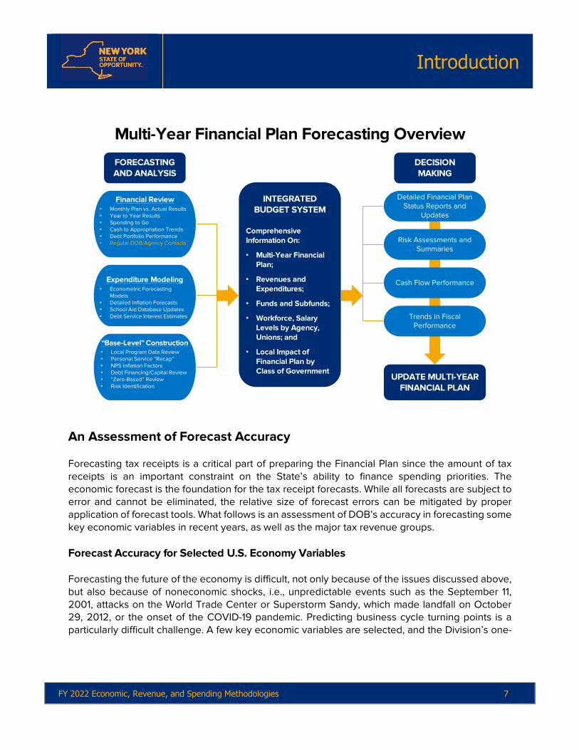
Multi-Year Financial Plan Forecasting Overview
FORECASTING AND ANALYSIS
Financial Review• Monthly Plan vs. Actual Results• Year to Year Results• Spending to Go• Cash to Appropriation Trends• Debt Portfolio Performance• Regular DOB/Agency Contacts
Expenditure Modeling• Econometric Forecasting
Models• Detailed Inflation Forecasts• School Aid Database Updates• Debt Service Interest Estimates
“Base-Level” Construction• Local Program Data Review• Personal Service “Recap”• NPS Inflation Factors• Debt Financing/Capital Review• “Zero-Based” Review• Risk Identification
INTEGRATED BUDGET SYSTEM
Comprehensive Information On:
• Multi-Year Financial Plan;
• Revenues and Expenditures;
• Funds and Subfunds;
• Workforce, Salary Levels by Agency, Unions; and
• Local Impact of Financial Plan by Class of Government
DECISION MAKING
Risk Assessments and Summaries
Cash Flow Performance
Detailed Financial Plan Status Reports and
Updates
Trends in Fiscal Performance
UPDATE MULTI-YEAR FINANCIAL PLAN
An Assessment of Forecast Accuracy Forecasting tax receipts is a critical part of preparing the Financial Plan since the amount of tax receipts is an important constraint on the State’s ability to finance spending priorities. The economic forecast is the foundation for the tax receipt forecasts. While all forecasts are subject to error and cannot be eliminated, the relative size of forecast errors can be mitigated by proper application of forecast tools. What follows is an assessment of DOB’s accuracy in forecasting some key economic variables in recent years, as well as the major tax revenue groups. Forecast Accuracy for Selected U.S. Economy Variables Forecasting the future of the economy is difficult, not only because of the issues discussed above, but also because of noneconomic shocks, i.e., unpredictable events such as the September 11, 2001, attacks on the World Trade Center or Superstorm Sandy, which made landfall on October 29, 2012, or the onset of the COVID-19 pandemic. Predicting business cycle turning points is a particularly difficult challenge. A few key economic variables are selected, and the Division’s one-

Introduction
8 FY 2022 Economic, Revenue, and Spending Methodologies
year-ahead annual forecast is compared to the initial BEA and BLS estimates.5 For comparison purposes, the Blue Chip forecast is also included where available. As the figures below indicate, forecast errors tend to be smaller when the economy is following a steady growth path than when the economy is changing direction. DOB’s forecast has tended to be very similar to the Blue Chip Consensus forecast for both real U.S. GDP growth and inflation. The Blue Chip consensus forecast and DOB both overestimated the strength of real U.S. GDP growth during the 2001 recession, but underestimated strength of the economy coming out. Neither DOB nor Blue Chip forecasters could have predicted the upcoming COVID-19 pandemic in their December 2019 forecast, therefore the forecast error for 2020 was very large. Similarly, the forecast error for employment was very large for 2020. The problems that energy price volatility presents in forecasting inflation are illustrated in the “Executive Budget Forecast Accuracy: US CPI (Consumer Price Index) Inflation One Year Ahead,“ shown below. Unlike the forecast error for real U.S. GDP, DOB's personal income forecast was below the actual growth in 2020. This was due to a record level of fiscal stimulus provided over the course of the year.
(4)
(3)
(2)
(1)
0
1
2
3
4
5
6
2000 2002 2004 2006 2008 2010 2012 2014 2016 2018 2020
Perc
ent C
hang
e
Blue ChipDOB ForecastActual
Executive Budget Forecast Accuracy: U.S. Real GDP GrowthOne Year Ahead
Note: “Actual” is based on BEA’s advance estimate for the fourth quarter, usually released at the end of the following Januaryexcept for 2018’s fourth quarter, which was released in February 2019 due to the government shutdown; Blue Chip and DOBforecasts for 2009 date from November 2008 due to the unusually early release date for the FY 2010 Executive Budget.
Source: Haver Analytics; Blue Chip Economic Indicators (December forecast for following year); Federal Reserve Bank ofPhiladelphia; DOB staff estimates.
5 Initial estimates rather than the most recent estimates are used as benchmarks to assess DOB’s forecast accuracy as forecasting future revisions to the data would be impossible.

Introduction
FY 2022 Economic, Revenue, and Spending Methodologies 9
(0.5)
0.0
0.5
1.0
1.5
2.0
2.5
3.0
3.5
4.0
4.5
2000 2002 2004 2006 2008 2010 2012 2014 2016 2018 2020
Perc
ent C
hang
eBlue ChipDOB ForecastActual
Executive Budget Forecast Accuracy: U.S. CPI InflationOne Year Ahead
Note: “Actual” is as of BLS’s preliminary estimate for December, released in the middle of the following January; Blue Chip andDOB forecasts for 2009 date from November 2008 due to the unusually early release date for the FY 2010 Executive Budget.
Source: Haver Analytics; Blue Chip Economic Indicators (December forecast for following year); Federal Reserve Bank ofPhiladelphia; DOB staff estimates.
(2)
(1)
0
1
2
3
4
5
6
7
2000 2002 2004 2006 2008 2010 2012 2014 2016 2018 2020
Perc
ent C
hang
e
DOB Forecast Actual
Executive Budget Forecast Accuracy: U.S. Personal IncomeOne Year Ahead
Note: “Actual” is based on BEA’s advance estimate of the fourth quarter, usually released at the end of the following Januaryexcept for 2018’s fourth quarter, which was released in February 2019 due to the government shutdown.
Source: Haver Analytics; Federal Reserve Bank of Philadelphia; DOB staff estimates.
Introduction
10 FY 2022 Economic, Revenue, and Spending Methodologies
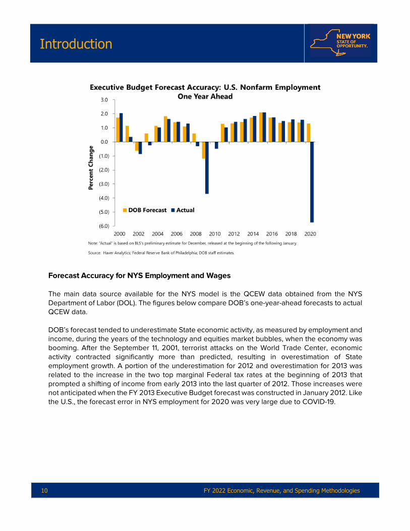
Forecast Accuracy for NYS Employment and Wages The main data source available for the NYS model is the QCEW data obtained from the NYS Department of Labor (DOL). The figures below compare DOB’s one-year-ahead forecasts to actual QCEW data. DOB’s forecast tended to underestimate State economic activity, as measured by employment and income, during the years of the technology and equities market bubbles, when the economy was booming. After the September 11, 2001, terrorist attacks on the World Trade Center, economic activity contracted significantly more than predicted, resulting in overestimation of State employment growth. A portion of the underestimation for 2012 and overestimation for 2013 was related to the increase in the two top marginal Federal tax rates at the beginning of 2013 that prompted a shifting of income from early 2013 into the last quarter of 2012. Those increases were not anticipated when the FY 2013 Executive Budget forecast was constructed in January 2012. Like the U.S., the forecast error in NYS employment for 2020 was very large due to COVID-19.

Introduction
FY 2022 Economic, Revenue, and Spending Methodologies 11
(11)
(10)
(9)
(8)
(7)
(6)
(5)
(4)
(3)
(2)
(1)
0
1
2
3
2001 2003 2005 2007 2009 2011 2013 2015 2017 2019
Perc
ent C
hang
e
DOB Forecast Actual
Executive Budget Forecast Accuracy: New York EmploymentOne Year Ahead
Source: NYS DOL; DOB staff estimates.
(4)(3)(2)(1)0123456789
10
2001 2003 2005 2007 2009 2011 2013 2015 2017 2019
Perc
ent C
hang
e
DOB Forecast Actual
Executive Budget Forecast Accuracy: New York WagesOne Year Ahead
Source: NYS DOL; DOB staff estimates.

Introduction
12 FY 2022 Economic, Revenue, and Spending Methodologies
Forecast Accuracy for Revenues As discussed, forecast models are simplified versions of reality and, as such, are subject to error. Tax collections in NYS are dependent on a host of specific factors that are difficult to predict accurately. A selection of more specific factors that either have affected or could affect NYS tax receipts estimates includes:
● National and State economic conditions, which are subject to shocks that are, by definition, unanticipated;
● One-time actions (that either accelerate or delay collections and thus impact cash flow);
● Court decisions concerning the proper applicability of a tax;
● State or Federal tax policy actions that could alter taxpayer behavior;
● Tax structures including tax rates and base subject to tax;
● Efficiency of tax collection systems;
● Enforcement efforts, audit activities and voluntary compliance;
● Timing of payments (shifting collections from one SFY to another);
● Tax Amnesty programs (1994, 1996, 2003, and 2010 covering PIT, corporate franchise tax
(CFT), sales tax, the estate and gift tax, and other minor taxes);
● Timing of Budget enactment; and
● Accounting changes mandated by statute. The Division's recent All Funds forecast performance are reviewed below with error defined as the actual collections minus the forecast. The “Enacted Budget Forecast Errors: Total Taxes” figure compares the total tax forecast with actual results and presents the historical pattern of the forecast errors (the FY 2010 forecast includes the estimated receipts for the Metropolitan Commuter Transportation Mobility tax which was established after the Enacted Budget). The overall pattern reflects the difficulty in forecasting at and near business cycle turning points and the tendency to overestimate receipts during recessions and to underestimate during expansions. The “Enacted Budget Forecast Accuracy: Forecast Errors” figure shows the share of the total dollar error contributed by each major tax category. In some years, there are offsetting errors. These figures also show that while an error rate may be significant, the dollars involved may be less so.

Introduction
FY 2022 Economic, Revenue, and Spending Methodologies 13
(6)
(4)
(2)
0
2
4
6
8
$0
$10
$20
$30
$40
$50
$60
$70
$80
$90
FY 2007 FY 2009 FY 2011 FY 2013 FY 2015 FY 2017 FY 2019 FY 2021
Percent ErrorBi
llion
s
Enacted Budget Forecast Actual Forecast Error (right scale)
Enacted Budget Forecast Errors: Total Taxes
Source: NYS DTF; DOB staff estimates.
($6)
($4)
($2)
$0
$2
$4
$6
$8
FY 2007 FY 2009 FY 2011 FY 2013 FY 2015 FY 2017 FY 2019 FY 2021
Billi
ons
PIT Consumption/Use Taxes Business Taxes Other Taxes
Enacted Budget Forecast Accuracy: Forecast Errors
Note: Error is defined as actual receipts less forecast receipts. Source: NYS DTF; DOB staff estimates.
Part I:
Economic Methodologies

Economic Methodologies
FY 2022 Economic, Revenue, and Spending Methodologies 15
The U.S. Macroeconomic Model DOB’s Economic and Revenue Unit provides projections on a wide range of economic and demographic variables which are used in the development of State revenue and expenditure projections, debt capacity analysis, and for other budget planning purposes. This section provides a detailed description of the econometric models developed by the staff for forecasting the national economy. Basic Features of the Model Drawing heavily on the methodology underlying the Federal Reserve Board’s macroeconomic model, DOB’s approach to modeling the U.S. economy incorporates the theoretical advances of the last 40 years in an econometric model designed for forecasting and policy simulation. The behavioral equations in DOB/US are consistent with economic agents that optimize their behavior subject to economically meaningful constraints. The model’s long-run equilibrium is the solution to a dynamic optimization problem carried out by households and firms. This approach permits both short-term business cycle fluctuations and long-term equilibrium properties to be handled within a consistent framework. This synthesis is made possible by adding adjustment frictions, as well as other departures from the perfectly competitive, instantaneous-adjustment model. The model structure also incorporates an error-correction framework that ensures movement back to equilibrium in the long run. Underlying this approach is a property of certain time series data called “cointegration,” under which certain types of time series share a tendency to return to a common equilibrium path, though they also may deviate from it for substantial periods. As in the Federal Reserve Board’s model, the assumptions that govern the long-run behavior of DOB/US stem from neoclassical microeconomic foundations, under which consumers exhibit maximizing behavior regarding consumption and labor-supply decisions, while firms maximize profit. In the long run the model solution converges to a balanced growth path. Consumption is determined by expected wealth, which is determined, in part, by expected future output and interest rates. The value of investment is affected by the cost of capital and expectations about the future paths of output and inflation. As even forward-looking economic agents do not adjust instantaneously to changing economic conditions, DOB/US incorporates dynamic adjustment mechanisms to deal with “frictions,” such as adjustment costs, the wage-setting process, and the persistent spending habits of consumers. Frictions delay the adjustment of nonfinancial variables, producing periods when labor and capital can deviate from optimal paths. These imbalances constitute signals that are important in wage and price setting because price setters must anticipate the actions of other agents. For example, firms set wages and prices in response to a set of expectations concerning productivity growth, available labor, and the consumption choices of households.

Economic Methodologies
16 FY 2022 Economic, Revenue, and Spending Methodologies
In contrast to the real sector, the financial sector is assumed to be unaffected by frictions, because transactions have negligible costs and well-developed primary and secondary markets for financial assets exist.6 It is now widely accepted that monetary policy can affect both inflation and the economy's equilibrium response to a real shock, and thus the course of the business cycle, thanks to this difference between the financial and real sectors of the economy. This leads to a consideration of how monetary policy is handled in DOB/US. By law, the monetary authority in the United States – the Federal Open Market Committee (FOMC), made up of the Federal Reserve’s Board of Governors plus five of the regional reserve bank presidents – has two mandates: to promote “maximum employment” and “stable prices.” While predicting the outcomes of committee meetings would appear impossible, it turns out that the “dual mandate” allows for the modeling of monetary policy decisions. DOB/US uses a modified “Taylor rule,” proposed by John Taylor.7 However, discretion is often used. For example, once the FOMC drove the target range for the federal funds rate to near-zero levels in trying to cope with the Great Recession, judgmental adjustments had to be used for modeling monetary policy, in place of reliance on the mechanical “Taylor rule.” Additional complications in modeling monetary policy have arisen from the FOMC’s use of unconventional policy tools, such as its communications and large-scale asset purchases, in the post-crisis period. Overview of Model Structure Well over 200 variables are forecast by the six modules of DOB/US. The first module estimates real potential U.S. output, measured by real U.S. GDP. The next module estimates agent expectations, which play a key role in determining long-term equilibrium values of important economic variables, such as consumption and investment, which are estimated in the third module. A fourth module produces forecasts for variables thought to be influenced primarily by exogenous forces but which play an important role in determining the economy’s other major indicators. The core behavioral model is the largest part of DOB/US and is its fifth block. Much of the discussion that follows focuses on this block which uses estimates from the third and fourth modules as inputs. The final module is made up of “satellite” models that use the core model variables as inputs, but do not feed back into the core behavioral equations. The current estimation period for the model is the first quarter (Q1) of 1965 through the fourth quarter (Q4) of 2019, excluding the COVID-19 period. Descriptions of each module follow below.
6 This assumption has recently been challenged considering the role of asset price bubbles in precipitating the credit crisis of 2008. Alternatively, bubbles can be viewed as resulting from long-term asset market frictions (see Markus Brunnermeier, Asset Pricing under Asymmetric Information: Bubbles, Crashes, Technical Analysis and Herding. Oxford, UK: Oxford University Press, 2001). 7 In the “Taylor Rule” framework, the policy decisions of the FOMC are guided by the extent to which inflation and output (the latter a proxy for employment) deviate from target levels. See John B. Taylor, “Discretion Versus Policy Rules in Practice,” Carnegie-Rochester Conference Series on Public Policy, vol. 39, 195-214, 1993.

Economic Methodologies
FY 2022 Economic, Revenue, and Spending Methodologies 17
Potential Output and the Output Gap Potential GDP is the output level the economy can produce when all available resources are utilized at their most efficient levels. It is the basis for the long-term equilibrium values and monetary policy forecasts of DOB/US. The economy can produce either above or below this level; when it does so for an extended period, economic agents can expect inflation to rise or fall, respectively, although the precise timing of that movement can depend on various factors. The “output gap” is the difference between actual and potential output. DOB’s method for estimating potential GDP largely follows that of the CBO.8 Potential GDP is estimated for each of the four major economic sectors defined under U.S. BEA NIPA data: private nonfarm business; private farm; government; and households and nonprofit institutions. A neoclassical growth model is specified for the nonfarm business sector (which makes up about 76 percent of GDP), incorporating three inputs to the production process: labor (measured by number of hours worked); capital stock; and total factor productivity (TFP). TFP cannot be directly estimated; instead, it is found as the residual from subtracting log output from a Cobb-Douglas production function (with fixed coefficients of 0.7 and 0.3 applied to log labor hours and log capital, respectively) from the historical log value of output. Each of the inputs to private nonfarm business production is assumed to have a component that varies with the business cycle, and to have a second, long-term, component that tracks the economy’s capacity to produce. Estimation of the long-term trend component presumes that the “potential” level of an input grows smoothly over time, though not necessarily at a fixed rate. Inputs are adjusted to their “potential” levels by estimating and then removing the cyclical component from the data series. For example, the cyclical component of the labor input is assumed to be reflected in the deviation of the actual unemployment rate from what economists define as the nonaccelerating inflation rate of unemployment, or NAIRU. When the unemployment rate falls below the NAIRU, indicating a tight labor market, the stage is set for higher wage growth and, in turn, higher inflation. The effect is reversed if the unemployment rate is above the NAIRU. After estimation, the fitted value from the regression is defined as the “potential level,” setting the unemployment rate deviations from the NAIRU equal to zero. This method is applied to all three of the major inputs to private nonfarm business production. To obtain a measure of potential private nonfarm business GDP, the potential levels of the three production inputs are substituted back into the production function where hours worked, capital, and TFP are given coefficients of 0.7, 0.3, and 1.0, respectively. For the other three sectors of the economy, the cyclical component is removed directly from the series using the method to estimate potential levels of the inputs to private nonfarm business production. Nominal potential values for the four sectors are also estimated by multiplying the chained dollar estimates by the implicit price deflators, based on quarterly historical data. The estimates for the four sectors are then “Fisher
8 Congressional Budget Office, “CBO’s Method for Estimating Potential Output,” October 1995, and Congressional Budget Office, “CBO’s Method for Estimating Potential Output: An Update,” August 2001.
Economic Methodologies
18 FY 2022 Economic, Revenue, and Spending Methodologies
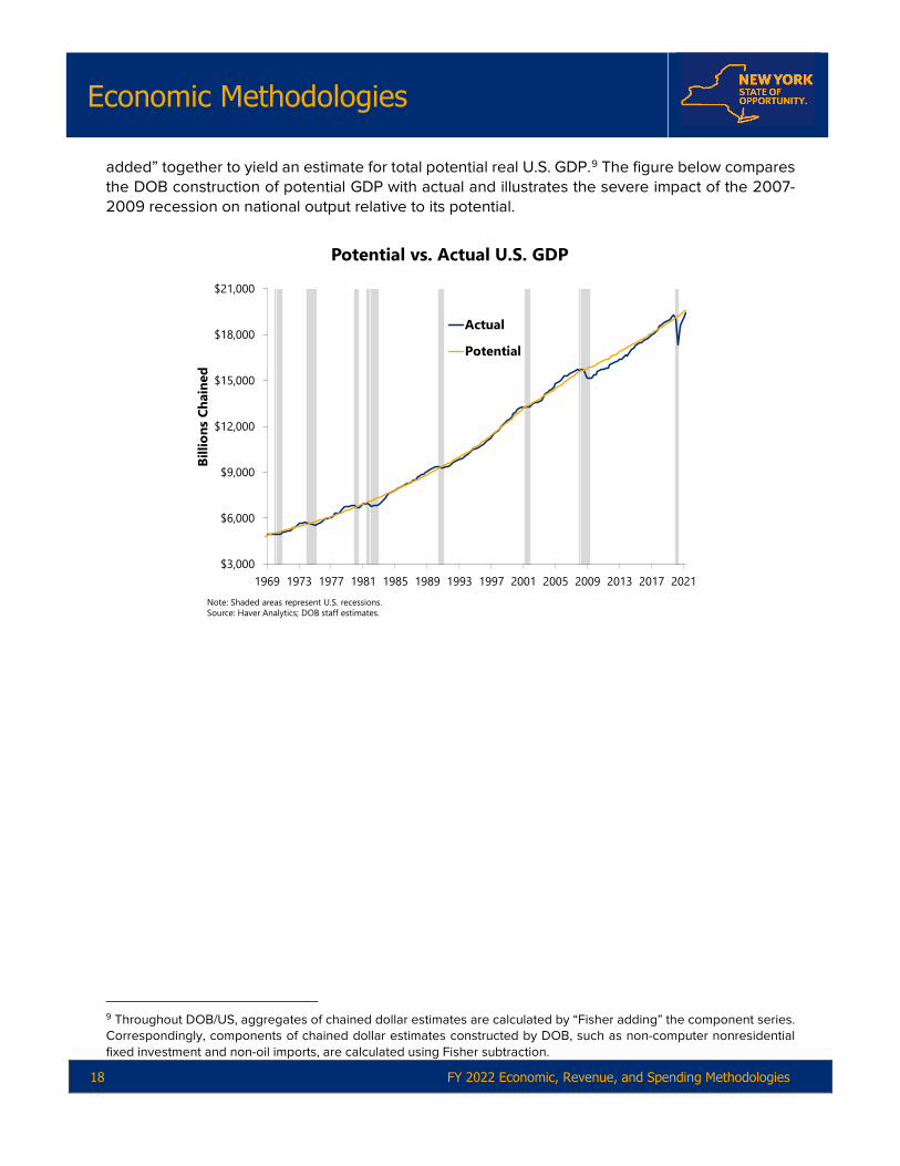
added” together to yield an estimate for total potential real U.S. GDP.9 The figure below compares the DOB construction of potential GDP with actual and illustrates the severe impact of the 2007-2009 recession on national output relative to its potential.
$3,000
$6,000
$9,000
$12,000
$15,000
$18,000
$21,000
1969 1973 1977 1981 1985 1989 1993 1997 2001 2005 2009 2013 2017 2021
Billi
ons
Chai
ned
Actual
Potential
Potential vs. Actual U.S. GDP
Note: Shaded areas represent U.S. recessions.Source: Haver Analytics; DOB staff estimates.
9 Throughout DOB/US, aggregates of chained dollar estimates are calculated by “Fisher adding” the component series. Correspondingly, components of chained dollar estimates constructed by DOB, such as non-computer nonresidential fixed investment and non-oil imports, are calculated using Fisher subtraction.

Economic Methodologies
FY 2022 Economic, Revenue, and Spending Methodologies 19
Expectations Formation Most important macroeconomic relationships are influenced by expectations. The general characteristics and policy implications of a full macroeconomic model will depend upon how expectations are formed. Rational and Adaptive Expectations Expectations play an important role in DOB/US in the determination of consumer and firm behavior. For example, when deciding expenditure levels, consumers are assumed to take a long-term view of their wealth prospects. Thus, when deciding how much to spend in a given period, they consider not only their current income but also their lifetime or “permanent income,” as per the “life cycle” or “permanent income” hypothesis put forward most famously by Milton Friedman.10 Producers are also assumed to be forward-looking, basing decisions on their expectations of future prices, interest rates, and output. However, since both households and firms experience costs associated with adjusting their long-term expenditure plans, both are assumed to exhibit a degree of behavioral inertia, adjusting only gradually. All economic agents in DOB/US are assumed to use all available information in forming their expectations, and that the expectations are correct, on average, over the long term. More formally, the rational expectations hypothesis (REH) implies that the expectation of a variable Y at time t, Yt, formed at period t-1, is the statistical expectation of Yt based on all available information at time t-1. However, because of evidence that agents adjust their expectations gradually, expectations in DOB/US are assumed to have an “adaptive” component as well, captured by including the term αYt-1, where α is hypothesized to be between zero and one. Consistent with the REH, it is assumed that agents’ long-run average forecast error is zero. This hybrid specification is inspired by Roberts,11 Rudd and Whelan,12 Sims,13 and others who argue that adaptive and rational expectations should not be viewed as mutually exclusive, particularly considering the high information costs associated with forecasting. Moreover, given the empirical importance of lags in forecasting inflation and other economic variables, it cannot be said that observable phenomena such as “habit persistence” and “price-stickiness” are model-inconsistent. DOB/US estimates agent expectations in two stages. First, expectations of three key economic variables (inflation, the federal funds rate, and percentage output gap) are estimated within a vector autoregressive (VAR) framework. These expectations become part of an information set that is shared by all agents who then use them to form expectations over variables that are specific to particular subsets of agents, such as households and firms. Details of this process are presented below.
10 Milton Friedman, A Theory of the Consumption Function, Princeton University Press for the National Bureau of Economic Research, Princeton, New Jersey, 1957. 11John M Roberts, “How Well Does the New Keynesian Sticky-Price Model Fit the Data?” The Federal Reserve Board, Finance and Economic Discussion Series 2001-13, (February 2001). 12 Jeremy Rudd and Karl Whelan, “Can Rational Expectations Sticky-Price Models Explain Inflation Dynamics?” The Federal Reserve Board, Finance and Economic Discussion Series 2003-46, (September 2003). 13 Christopher A. Sims, “Implications of Rational Inattention,” Journal of Monetary Economics, 50(3), 665-690 (April 2003).

Economic Methodologies
20 FY 2022 Economic, Revenue, and Spending Methodologies
Shared Expectations As previously discussed, all agents in DOB/US use a common information set to form expectations. The GDP price deflator is used as an inflation measure while the percentage output gap is defined as actual real GDP minus potential real GDP, divided by actual real GDP. Values for the early part of the forecast period are fixed by assumption, while values for the remaining quarters are estimated within a VAR framework, with the federal funds rate and the GDP inflation rate in first-difference form.
SHARED EXPECTATIONS VAR MODEL
7 8 9 10
11
0 1 2 3 4 5 6
12 13 14
0 1
2 3 41-1 -1
1 2 3 4
1 2 3 4
( ) ( )
( )
-
( )
t t ttt t
t t t t
t t t t
t
t
t
r
r r r r r rr
r r
∆α α α α α α α
β β
α ∆ α ∆ α ∆ α ∆
∆ ∆ ∆ ∆
α α α α ε
π∆π
π ππ π π πχ χ χ χ
∞ ∞
∞
− − −−
− − − −
− − − −
+
+
=
=
−
−
+ + + + ++ + + +
++ + + +
FederalFundsRate (
GDPDeflator
)
2 3 4 5 6
7 8 9 10
11 12 13 14
0 1 2 4 5 6
1 2 3 -4-1 -1
-1 -2 -3 4
1 2 -3 4
1 31 2-1= ( ) ( )
( )
( - )
-
t t t tt t
t t t t
t t t t
t tt tt t
t
r r r
r r r r
r r
β β β β β
β β β β
β β β β
χ
χ µ µ µ µ µ µ
ε
∆ ∆ ∆
π π ∆ ∆ ∆ ∆
∆π ∆π ∆π ∆π
χ χ χ χ
π π
∞
∞ ∞
+ − − −
−
− − −
− −− −
+ + + +
+ + + +
+ + +
−
+ +
+ + + + +Percentage Output Gap
7
8 9 10 11
12 13 14 15
-4
1 2 3 4
1 2 3 4
t
t t t t
t t t t t
rµ
µ µ µ µ
µ µ µ µ
∆
∆ ∆ ∆ ∆
χ χ χ χ ε
π π π π− − − −
− − − −
∞
++ + + ++ + + + +
Note: The subscript ' ' is used to indicate the endpoint condition; for the percentage output gap, the endpoint
tε condition stipulates a long-run value of zero. is the error term.
“Endpoint conditions” constrain the long-run values of these three variables. Endpoint restrictions for the federal funds rate and inflation are represented by the first two terms on the right-hand side of each equation in the table above, while the assumption that the percentage output gap becomes zero in the long run is implied and therefore does not appear explicitly in the equations. The endpoint condition for the federal funds rate is computed from forward rates. For inflation, the terminal constraint is the 10-year inflation rate expectation, as measured by survey data developed by the Federal Reserve Bank of Philadelphia.

Economic Methodologies
FY 2022 Economic, Revenue, and Spending Methodologies 21
(15)
(10)
(5)
0
5
10
15
20
1972 1976 1980 1984 1988 1992 1996 2000 2004 2008 2012 2016 2020
Perc
ent
Shared Expectations
GDP DeflatorPercentage Output GapFederal Funds Rate
Note: Shaded areas represent U.S. recessions. Source: Haver Analytics; DOB staff estimates.
Agent-Specific Expectations The common information set is augmented by expectations of agents in specific sectors. For example, since households base their consumption decisions on the expected lifetime accumulation of income and wealth, the household-specific information set includes expectations over the components of real disposable personal income and values of securities- and non-securities-related wealth. Similarly, the firm sector-specific information set includes expectations over the relative prices of investment goods. Long-Term Equilibrium Determination The economy’s long-term equilibrium is derived from a set of conditions that results from the optimizing behavior of economic agents, disregarding short-term adjustment costs. In the case of equilibrium consumption, households are assumed to be utility maximizers subject to a lifetime income constraint. Firms are assumed to maximize profits subject to a constant-returns-to-scale production function and are assumed to behave as price-takers. Equilibrium Consumption In the household sector, optimizing behavior is based on a life-cycle model whereby consumers maximize the present discounted value of their expected lifetime utility. Risk-averse consumers with unconstrained access to capital markets will tend to smooth their consumption spending over time, by borrowing, saving, or dissaving as circumstances demand, based on an estimate of “permanent income,” or their expected future lifetime resources. Expected permanent income is

Economic Methodologies
22 FY 2022 Economic, Revenue, and Spending Methodologies
comprised of the present discounted value of current and future real disposable income plus the value of household wealth. In DOB/US, the expected value of household permanent income for each quarter in the forecast period is approximated by a relatively stable share of expected potential GDP plus expected values for securities-related and nonsecurities-related wealth. The expected values for all the components of permanent income are determined in the agent-specific expectations module. Real disposable income is made up of several income sources, including labor income, property income (comprised of rental, interest, and dividend income), and transfer income. The precise composition of aggregate permanent income at any point in time will depend on the age profile of the U.S. household population, since the permanent income of younger households will contain a large share of labor income, while property and transfer income will dominate in the permanent income of older (retired) households. Since this age profile varies over time, the various components of permanent income enter the equation for long-term equilibrium consumption separately. In addition, this equation includes the current and lagged values of the output gap, capturing the notion that the rate at which households discount future income may depend on household perceptions of income risk, which in turn is assumed to vary with the business cycle. In DOB/US, the variation in long-term equilibrium consumption is assumed to be best approximated by the variation in those components of total consumption that tend not to exhibit extreme volatility over the course of the business cycle, namely services and nondurable goods.14 Equilibrium Investment in Producer Durable Equipment Most econometric models failed to contemporaneously capture the boom in nonresidential investment from 1992 to 2000, when it grew at an average annual rate of 11 percent. Tevlin and Whelan15 postulate two reasons for this. First, the average depreciation rate for producer durable equipment increased dramatically as computers grew as a share of the total, due to rapid advances in digital technology rendering computer and related equipment obsolete quickly. Indeed, the depreciation rate for computers and related equipment is more than twice that for other equipment.16 Second, investment became more sensitive to the user cost of capital. DOB/US estimates investment in computer equipment separately from the remainder of producer durable equipment due to these problems.17 The figure below compares the growth in the two investment components since 1990.
14 A “Fisher addition” of nondurable and services consumption produces the noncyclical component of total consumption. 15 Stacey Tevlin and Karl Whelan, “Explaining the Investment Boom of the 1990s,” Journal of Money, Credit, and Banking, 35(1), 1-22. (February 2003). 16 See Barbara M. Fraumeni, “The Measurement of Depreciation in the U.S. National Income and Product Accounts,” Survey of Current Business, U.S. Department of Commerce, pp. 7-23, (July 1997). 17 The brisk growth of computer equipment as a share of total producer durable equipment may represent in part an error in the data. Chain-weighting tends to overestimate real quantities when prices fall as quickly as those of computers and related equipment.

Economic Methodologies
FY 2022 Economic, Revenue, and Spending Methodologies 23
(40)
(30)
(20)
(10)
0
10
20
30
40
50
60
1990 1992 1994 1996 1998 2000 2002 2004 2006 2008 2010 2012 2014 2016 2018 2020
Perc
ent C
hang
e O
ne Y
ear A
go
Real Producer Durable Equipment Growth
ComputerNoncomputer
Note: Shaded areas represent U.S. recessions.Source: Haver Analytics; DOB staff estimates.
Profit-maximizing behavior dictates that the long-term rate of equilibrium investment is the rate of investment that maintains the optimum capital-output ratio. The optimal capital-output ratio will be proportional to the ratio of the price of output to the rental rate of capital, under a standard Cobb-Douglas production function. This holds for both types of producer durable equipment. Given this optimal ratio, desired growth in investment varies with output growth and changes in the rental rate of capital. For each type of equipment, the rental rate of capital is defined as its purchase price, represented by the implicit price deflator, multiplied by the sum of the financial cost of capital and the rate of depreciation. The financial cost of capital, a measure of the cost of borrowing in equity and debt markets, is estimated by giving equal weight to an estimate of the after-tax cost of equity and the yield on Moody’s Baa-rated corporate bonds.18 Different rates of depreciation are used for computer and noncomputer equipment. Equilibrium Prices, Productivity, Wages, and Hours Worked In equilibrium, the price level is determined by the condition that price equals marginal cost in competitive markets. Long-run productivity growth is determined by a time series model reflecting the belief that the best predictor of future growth is its own recent history. Long-term equilibrium nominal wage growth is determined by the sum of trend productivity growth and the long-term expected rate of inflation. The desired level of man-hours worked is constructed by dividing potential real GDP by trend labor productivity.
18 The series that estimates the after-tax cost of borrowing in the equity market is created by IHS Markit.

Economic Methodologies
24 FY 2022 Economic, Revenue, and Spending Methodologies
Exogenous Variables
There are many economic variables for which economic theory provides little or no guidance as to long-term or short-term behavior. The exogenous variable module estimates future values for over 30 such variables; their inputs are variables from the shared information set and autoregressive terms. Most exogenous variables are incorporated into identity equations that are used to compute NIPA concepts, although a few become inputs to the behavioral equations within the core behavioral module. The Core Behavioral Module
This module contains 133 estimating equations, 38 of which are behavioral. It contains five sectors: households, firms, government, the financial sector, and the foreign sector. The behavioral equations summarize the behavior of representative agents acting with foresight to achieve optimal outcomes in the presence of constraints. The short-run movement toward equilibrium is hampered by adjustment costs in the real sector. Agents plan to close the gap between the current level of variables and desired levels using a dynamic adjustment process. The magnitude of an adjustment made by agents during any given period is based on the size of the gap, past values of the variable, and past and expected values of other variables that may affect agents’ decisions. In the financial sector, agents are assumed to adjust instantaneously when new information becomes available. Therefore, equations for this sector do not contain any dynamic adjustment terms. Details on each of the five sectors follows. The Household Sector Consumption, housing investment, and labor supply are the main decision variables for households. Following Brayton and Tinsley,19 DOB/US assumes the existence of two groups of consumers. The larger class consists of forward-looking, utility-maximizing consumers whose consumption decisions are constrained by their permanent incomes. The model implicitly recognizes that this group is heterogeneous, representing various stages of the lifecycle. The second group is comprised of low-income households. Because they face credit-market constraints that prevent them from borrowing in order to smooth their consumption over time, they are called “liquidity constrained.” This also means that they are modeled as basing their consumption decisions only on current-period income.
19 Flint Brayton and Peter A. Tinsley, “A Guide to FRB/US, A Macroeconomic Model of the United States,” Macroeconomic and Quantitative Studies, Division of Research and Statistics, Federal Reserve Board (1996).

Economic Methodologies
FY 2022 Economic, Revenue, and Spending Methodologies 25
HOUSEHOLD SECTOR
C1 Real noncyclical consumption C2 Real cyclical consumption QC Desired real noncyclical consumption Y Real disposable personal income EZQC Expected desired noncyclical consumption EZGAP Expected potential GDP gap SLACB Willingness to lend to consumers INVH Residential fixed investment PSH Real new home price LIBOR3 3-month LIBOR rate GDPR Real GDP Ɛt Error Term
++τ +τ +ττ= τ= τ=
+τ=
= +
+
= +τ
∆ α α +α ∆ +α ∆ +α∑ ∑ ∑
+α ∆ α + α +
∆ β +β∑
ε
Noncyclical Consumption
Cyclical Consumption
0 1 2 3 4
5 6 7
0 1
5 5 5-1 -1
0 0 0
-3
5
0
ln 1 (ln -ln 1) ln 1 ( ln - )
ln 1980 2
ln 2 (ln -l
t t t t t t t
t t t t
t t
C EZQC QC C C Y EZQC EZGAP
Y D Q SLACB
C EZQC QC +
−
τ=+τ
β ∆ +β ∆
+β ∆ +β +β +β +β
+β +β +β +
∆ = µ + +µ +µ∑
ε
Residential Fixed Investment
2 3
4 5 6 7 8
9 10 11
0 1 2
-1 -1
1
5-1 -1
0
n 2) ln 2 ln
ln 1970 4 1974 4 1980 2 1981 4
1987 1 2001 4
( / )
t t t
t t t t
t t t t
t t
t
t t
C C Y
INVH D Q D Q D Q D Q
D Q D Q SLACB
INVH EZQC QC INVH INVH
−= +
+µ +µ ∆ +µ ∆ +µ +µ +µ +
θ + θ + θ ∆ θ ∆ +
ε
ε
Banks' Willingness to Lend to Consumers
3 4 5
0 1 2 3
6 7 8
1
1980 2 3 4 1976 4 1977 2
3 ln
t t t
t t t t t
tSLACB PSH Y D Q Q Q D Q D Qt t t
SLACB SLACB LIBOR GDPR
The four equations for the household sector incorporate expectations from either the shared information set VAR model or the agent-specific information set. The agent-specific information set for the household sector contains the expected value of wage and nonwage income, and the expected value of household wealth. The behavioral equations for the household sector balance the long-term equilibrium of theory with the empirically observed habit persistence and adjustment costs. The equations for the determination of cyclical consumption, noncyclical consumption, and housing investment appear above in the table titled “Household Sector.” Brief descriptions of the equations follow.

Economic Methodologies
26 FY 2022 Economic, Revenue, and Spending Methodologies
Consumption Consumption is divided into cyclical (durable goods) and noncyclical (services and nondurables) components, based on the significantly different growth rates these two groups display over the business cycle (see the figure titled “Cyclical vs Noncyclical: Real Consumption Growth” below). Noncyclical consumption is estimated using first differences of the logs of the data within a polynomial adjustment cost framework. The equation contains an error-correction term that captures the tendency toward long-run equilibrium; a lagged dependent variable that captures habit persistence; forward expectations of both desired noncyclical consumption and the output gap; bank willingness to lend to consumers; and real income (the last term meant to capture the behavior of liquidity-constrained households). The specification for cyclical consumption is very similar to that of noncyclical consumption, except for the exclusion of the error-correction and second expectations terms; the equation also includes real residential fixed investment, which tends to induce demand for household furniture, appliances, and other durable goods. Both equations contain dummy variables that account for extreme cyclical volatility and Federal policy shocks.
(15)
(10)
(5)
0
5
10
15
20
25
30
35
1969 1973 1977 1981 1985 1989 1993 1997 2001 2005 2009 2013 2017 2021
Perc
ent C
hang
e O
ne Y
ear A
go
Cyclical vs Noncyclical: Real Consumption Growth
NoncyclicalCyclical
Note: Cyclical refers to durable goods while noncyclical refers to nondurable goods and services. Shaded areas represent U.S.recessions.Source: Haver Analytics; DOB staff estimates.
Residential Fixed Investment Residential investment by households is estimated using a dynamic adjustment equation which assumes that households adjust their rate of housing investment in accordance with a long-term equilibrium relation between desired noncyclical consumption and housing services. A home price variable is also included in order to capture supply and demand features of the housing market.

Economic Methodologies
FY 2022 Economic, Revenue, and Spending Methodologies 27
Thus, the equation contains desired consumption divided by current housing investment; a lagged endogenous variable to capture habit persistence; forward-looking expectations of desired consumption; bank willingness to lend to consumers; and the real average purchase price of one-family homes. Bank Willingness to Lend Also appearing in the table above is the model for bank willingness to lend to consumers, using the concept from the Federal Reserve Board’s Senior Loan Officer Survey. This captures the impact on consumer spending of credit market conditions beyond the interest rate alone. The model specification for bank willingness to lend includes its own lag; the 3-month London Inter-Bank Offered Rate (LIBOR) to account for interbank lending costs; and real GDP growth (assumed to be inversely related to default risk). Labor Supply Households must make decisions about how much labor they will supply to the labor market. In DOB/US, the behavioral equation that determines the first difference of the labor force participation rate includes its own lags; real GDP lagged three quarters; a dummy variable capturing the influx of women into the labor market from the 1960s through 1980s; and dummy variables capturing the extraordinary increased hiring of federal government workers in the first quarters of 1990, 2000, and 2010, in order to conduct the Decennial Censuses. The labor supply is then determined by multiplying the labor force participation rate by an estimate of the working-age population (ages 16 through 64).

Economic Methodologies
28 FY 2022 Economic, Revenue, and Spending Methodologies
The Firm Sector DOB/US assumes that firms set their prices and factor input levels in order to maximize profits. This sector determines the following: the levels of the two components of nonresidential fixed investment in equipment; private nonresidential structures; investment in intellectual property products; labor demand; real wages; and output prices. Several of the firm-sector equations incorporate both error-correction terms to capture the impact of long-term equilibrium relationships, and dynamic adjustment terms to capture firm-level adjustment costs, like the household sector equations.
FIRM SECTOR: COMPUTER AND NONCOMPUTER EQUIPMENT
ττ
α α α α
α α α αα α ε
β
++=
∆ ∆ ∆
∆
∆
= + + +∑
+ + + +
+ + +
= +
Computer and Related Equipment
Noncomputer Equipment
0 1 2 3
4 5 6 7
8 9
0
5-1 -1
0
-1
( - )
2 2008 3 2008 4
2009 4 1
t t t t t
t t t t
t t t
t
lCO EQICO QlCO lCO lCO POTGDP
RRC Y KD D Q D Q
D Q AR
lEXCO EQ ττ
β β
β β β ε
+=
∆
∆
+ +∑
+ + + +
1 2
3 4 5
5-1 -1
0
-1
( - )
2
t t t
t t t t
IEXCO QIEXCO lEXCO lEXCO
GDPGAP RRO Y KD
ICO Nonres. fixed investment – computer and related equipment EQICO Expected desired computer investment QICO Desired computer investment – durable equipment POTGDP Potential GDP RRC Rental rate of capital– computers Y2KD Post-Y2K dummy for 2001 D2008Q3 Dummy for 2008Q3 D2008Q4 Dummy for 2008Q4 D2009Q4 Dummy for 2009Q4 AR1 First-order autocorrelation correction IEXCO Nonres. fixed investment – durable equip. excl. computers EQIEXCO Expected future desired investment – durable equip. excl. computers QIEXCO Desired investment – durable equip. excl. computers GDPGAP Percent real GDP gap RRO Rental rate of capital – other durable equipment Ɛt Error Term

Economic Methodologies
FY 2022 Economic, Revenue, and Spending Methodologies 29
FIRM SECTOR: STRUCTURES AND INTELLECTUAL PROPERTY PRODUCTS
2 3
0 1 2 3 4
5 6 7 8
0 1
-1 -2 -3
-1
ln ln ln ln ln
ln 1986 2 2001 4 1978 2
ln ln 2 lnt
t t t t t
t t t t t
t t tt
lS lS lS GDP RRS
RRO D Q D Q D Q
lIPP lIPP Y KD POTGDP
α α α α α
α α α α
β β β β
ε
ε
∆ ∆ ∆ ∆ ∆
∆
∆ = ∆ ∆
= + + + +
+ + + + +
+ + + +
Structures
Intellectual Property Products
IS Nonres. fixed investment – structures GDP Real GDP RRS Rental rate of capital – structures RRO Rental rate of capital – other durable equipment D1986Q2 Dummy for Tax Reform Act of 1986 D2001Q4 Dummy for retroactive provision of Job Creation and Worker Assistance Act of 2002 D1978Q2 Dummy for 1978Q2 IIPP Nonres. fixed investment – intellectual property products Y2KD Post-Y2K dummy for 2001 POTGDP Potential GDP Ɛt Error Term
Nonresidential Investment DOB/US estimates four categories of real nonresidential investment: investment in computer-related producer durable equipment; investment in all other equipment; investment in nonresidential structures; and investment in intellectual property products. The estimating equations for investment in computer and related equipment and all other equipment are virtually identical. Both equations contain an error-correction term, defined as a lag difference between equilibrium and current investment; an autoregressive term; forward expectations of equilibrium investment; and the appropriate rental rate of capital, as defined above. The computer equipment equation contains the first difference of potential GDP growth; a dummy variable to capture the large decline in investment during the second and third quarters of 2001, as well as other dummies. The equation for noncomputer equipment contains the current period value of the output gap. Investment in nonresidential structures is determined by its own past values; real U.S. GDP growth; its own rental rate and the rental rate of noncomputer equipment; and dummy variables. Investment in intellectual property products is determined by its own past value, the first log difference of potential GDP growth, and a dummy variable to capture the large decline in investment during the second and third quarters of 2001. Labor Demand: Hours Worked and Employment In DOB/US, the level of national employment is determined by estimating equations for the number of hours worked and the length of the average workweek, which together capture the nonfarm

Economic Methodologies
30 FY 2022 Economic, Revenue, and Spending Methodologies
private business sector’s demand for labor. Total employment, in turn, affects the movements of many other economic variables, such as output, wages, consumption, and inflation. Hours worked are estimated using a dynamic adjustment equation that includes an error-correction term composed of the difference between long-term equilibrium hours and actual hours; real U.S. GDP growth; the expected one-period-ahead value of the output gap; and dummy variables. The estimating equation for the average length of the workweek in the private nonfarm business sector also contains an error-correction term and the expected one-period-ahead value of the output gap. In addition, the model includes growth in real private nonfarm business GDP and dummy variables. The level of total private nonfarm employment is determined by dividing hours worked by the average length of the workweek multiplied by the number of weeks in a year. The Wage Rate The average hourly wage rate is defined as total private employee compensation (cash wages and salaries plus additional costs such as medical insurance premiums and employer contributions for social insurance) divided by hours worked. The long-run equilibrium growth in the wage rate is assumed to depend on trend productivity growth and the inflation rate, where inflation is measured by the private nonfarm chain-weighted GDP deflator and productivity is private nonfarm output divided by hours worked, adjusted to remove the effects of the business cycle. Thus, the equilibrium wage rate at time t is its value at time t-1 plus the sum of the growth rates for productivity and inflation. The actual quarterly wage rate is modeled in an error-correction framework but contains additional lags capturing the presence of “wage-stickiness.” The model also includes the expected one-period-ahead value of the output gap to capture the impact of forward-looking behavior on the speed of adjustment toward equilibrium. Output Prices The price level is represented by the private nonfarm chain-weighted GDP deflator. Its growth is modeled within a dynamic adjustment framework in which the price level adjusts gradually from its current level to its long-term equilibrium value. The model also includes the expected one- and two-period-ahead values of the output gap, again to capture the impact of forward-looking behavior on the speed of adjustment toward equilibrium. In addition, the model contains the petroleum products component of the Producer Price Index (PPI) to capture the impact of wholesale energy prices, as well as dummy variables to capture the impact of the 1970s oil shocks above and beyond what the PPI captures. Monetary Policy and the Financial Sector Monetary policy affects economic and financial decisions made by agents in the economy. The objective of monetary policy is to stabilize the economy’s performance – as reflected in the behavior of inflation, output, and employment – by balancing the twin goals of full employment and price stability. This is accomplished by raising or lowering short-term interest rates through changes in the central bank’s target federal funds rate in a manner that is consistent with its twin goals.

Economic Methodologies
FY 2022 Economic, Revenue, and Spending Methodologies 31
(4)
(2)
0
2
4
6
8
10
1990 1992 1994 1996 1998 2000 2002 2004 2006 2008 2010 2012 2014 2016 2018 2020
Perc
ent
Federal Funds Rate
Taylor's Rule
Note: Shaded areas represent U.S. recessions.Source: Haver Analytics; DOB staff estimates.
Federal Funds Rate vs. Rate Implied by Taylor's Rule
Within DOB/US, monetary policy is administered through a modified version of Taylor’s monetary rule. As illustrated in the figure above, “Federal Funds Rate vs. Rate Implied by Taylor’s Rule,” Taylor’s rule approximates the way the Federal Reserve has historically conducted monetary policy, particularly when the classic rule is augmented by expectations over future inflation and output. Note however the large deviations from the rule as a result of the “zero lower bound” on the federal funds rate in the period during and after the Great Recession. Deviations from the Federal Reserve’s assumed inflation target are weighed twice as heavily as deviations from its output growth target. In addition, the contemporaneous value of inflation is replaced by an average of actual inflation for the past three quarters and expected inflation for both the current quarter and the quarter ahead. A similar modification is made to the output growth term. This modified specification makes operational the requirement that the central bank be able to project the effect of its policy alternatives on the output gap and inflation and that its policy choice be consistent with that projection. The DOB/US specification of Taylor’s rule appears in the table labelled “Monetary Policy: Taylor’s Rule.” The financial sector of DOB/US is subdivided into two blocks of equations: one determining equity prices and the other determining interest rates. Many analysts believe that short-run changes in stock market prices follow a random walk and therefore day-to-day movements of individual stocks are impossible to forecast with any accuracy. However, long-run movements in price indices of large groups of stocks appear to move systematically with other economic variables. Much of the variation in the growth of the S&P 500 stock price index can be explained by the contemporaneous and expected growth of pre-tax corporate profits after normalizing by the interest rate on Baa corporate bonds. A lead term is added to capture the influence of profit expectations on investors’ decisions to buy and sell equities, and, subsequently, on stock prices.

Economic Methodologies
32 FY 2022 Economic, Revenue, and Spending Methodologies
In addition to the federal funds rate, which is modeled based on Taylor’s rule, DOB/US contains models for six interest rates: the three-month, one-year, five-year, and ten-year U.S. Treasury yields, as well as the Baa corporate bond rate and the 30-year conventional mortgage rate. These equations are specified within an error-correction framework based on the expectations theory of the term structure of interest rates, which posits that the yield on the long-term bond equals the expected yield on a series of short-term bonds over the life of the long-term bond, plus term and risk premiums. The theory implies that the rate on one-year government bonds can be used to explain the rate on five-year bonds, which, in turn, is used to explain the rate on bonds of longer maturities. Although the term and risk premiums are not explicitly captured in the estimated model, their impacts are embodied in the estimated coefficients. A real GDP gap term is added to most of the equations in order to capture the impact of expected (future) inflationary pressures on the current yield curve. Adjustments are made to account for the anticipated impact of the Federal Reserve’s less traditional policies, such as quantitative easing and “Operation Twist.”
MONETARY POLICY: TAYLOR’S RULE
rT Federal funds target rate GDP growth rate Average GDP inflation Average GDP growth rate R Real rate of interest GDP target growth rate GDP inflation r Federal funds market rate Inflation target
The Government Sector DOB/US also contains equations that estimate the contribution to GDP from Federal, and state and local governments. Spending by both the Federal government and state and local governments depends on the revenues they collect. Although government revenues come from various sources – PIT, sales taxes, corporate business taxes, and fees – we find that PIT receipts act as an adequate proxy for receipts from all these sources. Since the components of personal income grow at varying rates, the models for both Federal and state and local revenues include these components separately, as well as effective tax rates. All government sector variables are modeled in first-differenced logarithmic form. Since government receipts are only available in nominal terms, final demand by the government sector is modeled in nominal terms as well. Real spending is calculated by deflating these nominal
13 2 1
3 2 1 1
1 0.5( ) ( )
5
5,
T t t t T t T
tt
t
t t t
t t t
t t t t t
t
r R g g
g g g g gg
where R r
π π ππ π π π ππ
π
−− − +
− − − +
= + + − + −+ + + +
=
+ + + +=
= −
g
π g
Tgπ
Tπ
Economic Methodologies
FY 2022 Economic, Revenue, and Spending Methodologies 33
values by the appropriate price deflators. Because governments determine their budgets before they know how much revenue they will collect, they do not adjust quickly to current revenue shocks. In addition, Federal government spending is not constrained in the short run by current-year revenue. Therefore, government spending models include past revenue with lags up to seven quarters, as well as the current period nonfarm GDP price deflator. The Federal government spending model also includes the percentage GDP gap, capturing the countercyclical nature of some government spending, and government employment, since employee compensation accounts for most of the state and local government contribution to final demand. In addition, DOB/US estimates the impact of changes in fiscal policy on the macroeconomy. Because the primary determinant of consumer spending is households’ long-term expectations of disposable income, modeling the impacts of fiscal policy plays an important role in forecasting household consumption when there is a policy change, an example of which was the expiration of the payroll tax holiday at the end of 2012. To accomplish this, DOB/US combines the most recent Joint Committee on Taxation20 and CBO estimates (where available) with results from Current Expenditure Survey data, disaggregated by income level, to estimate how much of the change in disposable income will affect consumption. The Foreign Sector Real U.S. exports are determined by the level of foreign economic activity, as measured by an estimate of the growth rate of global GDP, and by U.S. export prices relative to foreign prices. Real imports are divided into non-oil and oil goods and services. Non-oil imports are a function of real domestic demand and the ratio of import prices to domestic prices. Oil imports are a function of real domestic demand, as well as oil prices relative to domestic prices. Both imports and exports equations contain additional dummy variables to capture one-time shocks, such as the September 11, 2001 terrorist attacks on the World Trade Center and the oil-price shocks of the 1970s. Satellite Models DOB/U.S. includes satellite models that use variables from the core model as explanatory variables to forecast additional concepts, which do not feed back into the core behavioral equations discussed above. Sectoral Employment Total employment is disaggregated into 20 industrial sectors based on NAICS. Individual equations incorporate “structural” variables that are forecast in prior modules, such as hours worked, real GDP, real personal income, the inflation-adjusted S&P 500, interest rates, and demographic variables. The general approach is to estimate an error-correction model, although the error-correction term is dropped if it is not significant. To remove seasonality, some of the sectors are modeled in year-ago differences. To capture seasonality in those sectors that are modeled in first
20 The Joint Committee on Taxation is a nonpartisan committee of the U.S. Congress, originally established under the Revenue Act of 1926. For further information, see https://www.jct.gov/about-us/overview.html.

Economic Methodologies
34 FY 2022 Economic, Revenue, and Spending Methodologies
differences, we add time-varying seasonal dummy variables, which are constructed using the X11 procedure developed by the U.S. Census Bureau. Nominal Consumption Detail DOB forecasts 16 detailed components of nominal consumption expenditures for the purpose of forecasting sales tax receipts (see the Sales and Use Tax section of this Volume). Three examples of these forecasting models follow in the “Selected Consumption Models” figure on the next page. All models are in first-differenced log form. The three major components of consumption expenditures are durable goods, nondurable goods, and services. To help ensure that the detailed components add up to projected totals, either the total or a function of the total appears on the right-hand side and is retained if the coefficient is statistically significant. For example, total durable consumption spending minus spending on motor vehicles and parts is on the right-hand side of furnishings and durable household equipment spending. Also included are its own lagged value; fixed residential investment; bank willingness to lend; and some dummy variables to account for large shocks that cannot be accounted for by the other explanatory variables. Given that credit-market conditions are already accounted for to some extent by total durable spending, the negative coefficient on bank willingness to lend may be an indication that this component is less sensitive to credit market conditions than the total less spending on motor vehicles and parts. The model specification for consumer spending on gasoline and other energy goods includes total nondurable consumption, of which it is a component; the energy goods component of the PPI for finished goods; and bank willingness to lend. The model specification for consumer spending on transportation services includes total services consumption less spending for medical, housing, and financial services; the energy goods component of the PPI for finished goods; bank willingness to lend; and total private sector employment (to capture changes in aggregate demand).

Economic Methodologies
FY 2022 Economic, Revenue, and Spending Methodologies 35
SELECTED CONSUMPTION MODELS
( )
( )
−
−
∆ = α + α ∆ − + α ∆ + α ∆
+α α + α +
∆ = β + β ∆ + β ∆ + β +
∆ = µ + µ ∆ − − − µ ∆
+µ
+ ε
ε
+
t t t t
t t t t
t tt t t
t t t t t t
tCDFHEQ CD CDMVPQ IFIXR CDFHEQSLACB D Q D Q
CNGFOQ CN WPI SLACB
CSTRSQ CS CSMEDQ CSHHOQ CSFIQ WPI
0 1 2 3
4 5 6
0 1 2 3
0 1 2
2
1
ln ln ln ln1986 4 1989 1
ln ln ln 057
ln ln ln 057
−∆ + µ + µ ∆ + εt t t tCSTRSQ SLACB EEAP3 4 51ln ln CDFHEQ PCE: Furnishings and Durable Household Equipment CD PCE: Durable Goods CDMVPQ PCE: Motor Vehicle and Parts IFIXR Residential Investment SLACB Willingness to lend to consumers D1986Q4 Dummy (=1 for 1986Q4; 0 otherwise) D1989Q1 Dummy (=1 for 1989Q1; 0 otherwise) CNGFOQ PCE: Gasoline and Other Energy Goods CN PCE: Nondurable Goods WPI057 PPI: Finished Energy Goods SLACB Willingness to lend to consumers CSTRSQ PCE: Transportation Services CS PCE: Services CSMEDQ PCE: Medical Services CSHHOQ PCE: Housing Services CSFIQ PCE: Financial Services EEAP U.S. Private Employment Ɛt Error Term
Other Prices The nonfarm private GDP deflator and other deflators from the core model are used to forecast several implicit price deflators for consumption, as well as the overall CPI and some of its components. The PPI for refined petroleum products and other implicit price deflators for consumption are used to forecast several components of the PPI. Nonpersonal Service Inflation DOB provides forecasts for 36 detailed price components specifically for the purpose of forecasting the nonpersonal service (NPS) expenditure component of the State budget. Since these forecasts are used by many different units within DOB for fiscal planning purposes, most are modeled on a State fiscal year basis. This set of forecast variables includes price deflators for

Economic Methodologies
36 FY 2022 Economic, Revenue, and Spending Methodologies
medical equipment; office equipment; office supplies; energy-related products; business services; and real estate rentals. Right-hand-side variables for these models include the DOB/US forecasts for price indices described above. For example, the price index for light fuel oil explains much of the variation in the index for home heating oil. Likewise, the price index for medical equipment is well represented by the price index for total medical care excluding medical services and drugs and medical supplies. All three of the latter measures are forecast within DOB/US. The figure that follows presents the model specifications for two of these price series.
SELECTED PRICE DEFLATORS
0 1
0 1 2 3 4
ln 057302 ln 0573
ln ln ln ln
t t
t t t t
t
t
WPI WPI
CPIUEMB CPIMED CPISVMED CPIUEMA d
εα α
β β β β β ε
∆ ∆
∆ ∆ ∆ ∆
= + +
= + + + + +
Home Heating Oil
Medical Equipment1995
WPI057302 PPI: Fuel oil #2 home heating oil WPI0573 PPI: Light fuel oils CPIUEMB CPI: Medical equipment CPIMED CPI: Medical care CPISVMED CPI: Medical services CPIUEMA CPI: Drugs and medical supplies Ɛt Error Term
Other Interest Rates and the Wilshire 5000 DOB/US also estimates eight additional interest rates, including commercial paper rates; Treasury bond rates; state and local municipal bond rates; LIBOR rates; and mortgage rates. These are estimated in single-equation models using variables from the core model as inputs. The Wilshire 5000 stock price index is estimated using the S&P 500 stock price index as an explanatory variable. Miscellaneous Variables The models discussed above, as well as the NYS model, provide inputs to the forecasts of many miscellaneous variables, such as average price of new light vehicles. These miscellaneous variables are forecast based on single-equation models.

Economic Methodologies
FY 2022 Economic, Revenue, and Spending Methodologies 37
Current Quarter Estimation The DOB/US macroeconomic models described above are all quarterly models, consistent with their primary data source, the BEA’s NIPA data. However, BEA’s quarterly estimates are themselves based on data compiled (generally at a monthly frequency) by the U.S. Department of Labor’s BLS; the U.S. Department of Commerce’s Census Bureau; and the BEA itself. Much of these data – though not all – are reported to the public. The purpose of DOB’s current-quarter tracking system is to make maximum use of the available high frequency information at the time a forecast is made. This allows DOB to estimate more accurately the base quarters for both real and nominal GDP, as well as personal income. Since the DOB/US models discussed above tend to project equilibrium relationships assuming no exogenous shocks, the projected annual growth rate for the near term is heavily dependent upon the base quarter estimate. The accuracy of the base quarter is crucial to the accuracy of the overall forecast. The BEA produces three estimates in the months immediately following the quarter being estimated – an initial release followed by two revisions. DOB always incorporates the most recent NIPA data when doing a forecast. DOB’s current quarter methodology is designed to incorporate the full breadth of the available high frequency data to forecast the advance release of either the quarter in progress or just ended. These data include monthly payroll employment; the value of construction put in place; weekly initial unemployment insurance claims; and monthly personal income and personal consumption estimates, to name just a few. Mixed-Data Sampling (MIDAS) Current Quarter Model Traditional methods of current quarter forecasting are constrained by the use of variables of the same frequency. However, with a variety of economic variables available at different frequencies, potentially valuable information is lost under these methods as the details of higher frequency series are often discarded. For example, GDP is reported on a quarterly basis, whereas employment is reported monthly, and interest rates are reported daily. There have been different approaches to estimating low frequency variables using high frequency series. One approach uses the average (or sum) of the high frequency series in the regression equation for the low frequency variable, applying equal weighting to each value in the average (or sum). A second approach is to include the high frequency series in the regression but allowing for a separate coefficient for each high frequency component, for example, using separate regressors for each month. However, this approach may require the estimation of a large number of coefficients. Mixed-Data Sampling (MIDAS) estimation combines these two approaches allowing for the independent and dependent variables to be sampled at different frequencies. Given the wealth of high-frequency economic data, the MIDAS approach is ideal for the estimation of lower-frequency current quarter variables. For example, the following table specifies the employment module of DOB’s U.S. Current Quarter Model which includes both monthly and weekly regressors.

Economic Methodologies
38 FY 2022 Economic, Revenue, and Spending Methodologies
U.S. EMPLOYMENT CURRENT QUARTER MODEL
0 1 2 3 4
5 6
1
/4
( 1)/4
({ }, )
({ }, )
t t t t t
t t tw
t tw
t t
TOTEMP TOTEMP STRIKE ISMC CENSUS
LICM LIUM
LICM LICM
LIUM LIUM
f
f
−
−
∆ = ∆ + ∆
∆
α α α α + α
+ α + α +
= θ
= θ
+ +ε
TOTEMP Nonfarm payroll employment STRIKE Employees on strike ISMC ISM Composite Index (Manufacturing + Services) CENSUS Employees working temporarily on Census LICMf Initial UI claims (f=w weekly frequency, monthly otherwise) LIUMf Continuing UI claims (f=w weekly frequency, monthly otherwise) Ɛt Error term
U.S. nonfarm payroll employment is a very important monthly indicator as it is used to forecast wages, which is the largest component of personal income. DOB’s model uses initial unemployment insurance (UI) claims and continuing UI claims as the main predictors for payroll employment. Initial claims reflect layoffs, while continuing claims measure the accumulation of individuals no longer in the workforce and, thus, can serve as a proxy for hiring activities.21 Increases in initial and continuing claims indicate weaker employment growth, while decreases suggest an improving labor market. Additional predictors for this model include ISM Composite Index, the change in the number of workers striking during the month (to correct for volatilities in historical data due to strikes), and the change in the number of workers temporarily employed by the Federal government to conduct the Decennial Census. Unemployment insurance claims are used to estimate payroll employment in monthly frequency, while initial and continuing claims are estimated using the MIDAS method. Monthly claims are described as functions of weekly claims and their lags, weighted by a chosen MIDAS weighting function. In this model, the polynomial distributed lags (PDL/Almon) weighting is selected, in which each lag has a distinct coefficient θi approximated using a polynomial function of i. Due to the rolling release of weekly claims data each month, different number of lags in the MIDAS equations are used depending on the extent of data availability at the time of forecast. In doing so, DOB preserves the detail of each high frequency datapoint, and maximizes the robustness of the model as more weekly datapoints become available. Forecasting Challenges During COVID-19 Macroeconomic forecasting has always been and will always be challenged by unforeseeable adverse events – rising oil prices due to the eruption of conflict in the Middle East or natural disasters. However, the impact of the COVID-19 pandemic dwarfs any such events that have taken place since the financial crisis of 2008. The result has been an unprecedented number of business
21 A decline in continuing claims could also be due to people exhausting their UI benefits defined by law.

Economic Methodologies
FY 2022 Economic, Revenue, and Spending Methodologies 39
closures and job losses, long production and shipment delays, and the largest Federal stimulus programs in recent history. U.S. real GDP contracted by an annualized rate of 31.2 percent in the second quarter of 2020, more than three times greater than what had been the largest annualized quarterly drop in the history of the current series, which goes back to the first quarter of 1947. The subsequent rebound in the third quarter produced growth of 33.8 percent, more than double what had until then been the largest quarterly increase in the history of the series. Similarly, the unemployment rate surged from 3.5 percent in February 2020 to 14.8 percent in April, the largest two-month increase in the history of the current seasonally adjusted series, going back to early 1947. With the economy rapidly adapting to the realities of the pandemic in historically unprecedented ways – consider the widespread embrace of remote work – even short-term forecasting has become unusually challenging using conventional methods. Recent academic research offers several alternative approaches to improving forecast accuracy under the current circumstances.22 In summarizing some of these innovative approaches, Ho (2021) emphasizes two, the first being the use of “subjective judgment” to modify existing models, based on explicit assumptions about how model dynamics might differ from past experience. As an example, there is little doubt that the historical pattern of co-movement between leisure and hospitality sector employment and jobs in other sectors has been totally disrupted by the pandemic. With the economic impact of the pandemic unfolding in real time, in some cases months before being accounted in the quarterly national and state data that typically underly DOB’s macroeconomic models, a second approach cited by Ho (2021) is the incorporation of novel high frequency data that may help to gauge the state of the economy and improve forecasts. In addition to regularly published government data such as weekly unemployment insurance (UI) claims, Chetty et al. (2020) developed a publicly available database containing both daily and weekly data to track how the pandemic was affecting consumer spending, employment, small business revenues, and other economic indicators, based on data collected from credit card processing firms, payroll companies, and other sources.23 Although high frequency data enable forecasters and policymakers to track the economy with a much shorter lag, some of these series suffer from short history, and irregular or missing data, which can certainly contribute to the size of the resulting forecast errors. Ho (2021) documents that it is informative to use such data only to the extent that the relationships between the high frequency series and the variables being forecast are appropriately modeled. In addition to crafting explicit assumptions as to how the pandemic is likely to affect the co-movements among key variables, as well as the enhanced use of high-frequency data, DOB
22 Ho, Paul (2021) “How Macroeconomic Forecasters Adjusted During the COVID-19 Pandemic,” Federal Reserve Bank of Richmond Economic Brief, No 21-19, (June 2021) and Ho, Paul “Forecasting in the Absence of Precedent,” Federal Reserve Bank of Richmond Working Paper Series, WP 21-10, (June 2021). 23 Chetty, Raj, J. Friedman, N. Hendren, M. Stepner, and The Opportunity Insights Team, “The Economic Impacts of COVID-19: Evidence from a New Public Database Built Using Private Sector Data,” National Bureau of Economic Research, NBER Working Paper 27431, (November 2020).

Economic Methodologies
40 FY 2022 Economic, Revenue, and Spending Methodologies
modified its macroeconomic models in other ways to improve forecast accuracy in the age of COVID-19. DOB/US excludes the COVID-19 era from its estimation period, precluding the need for dummy variables to correct for pandemic-related volatility. In contrast, longer time lags in the availability of data led to a different approach to forecasting state-level variables. DOB/NY was re-estimated and dummy variables were added to selected equations to capture the impact of the pandemic on the New York economy.
(9)
(6)
(3)
0
3
Jan-20 Mar-20 May-20 Jul-20 Sep-20 Nov-20
Perc
ent C
hang
e
Evolution of Blue Chip ForecastsReal GDP Growth for 2020
Mean Bottom 10% Top 10%
Actual = -3.5%
Source: Blue Chip Economic Indicators.
The figure above charts the evolution of the Blue Chip Consensus forecast for U.S. real GDP for 2020 over the course of the year. It is illuminating that even as late as August 2020, with two quarters of data available, the ultimate actual decline of 3.5 percent is not even within the range between the averages over the top and bottom 10 percent of forecasts, underscoring the profound level of uncertainty that currently characterizes the macroeconomic forecasting enterprise. Therefore, despite all the efforts described above, this uncertainty is likely to persist well into the future.

Economic Methodologies
FY 2022 Economic, Revenue, and Spending Methodologies 41
New York State Macroeconomic Model
DOB’s macroeconomic model for NYS attempts to capture the fundamental linkages between the State and national economies. In general, the State’s economy grows in tandem with the national economy, and contracts when the nation is in recession. But the relationship is more complicated. The figure below compares the lengths of the national recessions, as defined by the NBER Business Cycle Dating Committee, with those of the State, as determined by the NY Index of Coincident Economic Indicators (constructed by DOB) and shows that the length and severity of the State’s recessions can differ from those of the nation.24 Due to the disproportionate impact of the September 11, 2001, terrorist attacks on the World Trade Center, the State came out of the 2001 recession significantly later than the nation. In contrast, NYS entered the 2008 recession eight months after the nation and exited the downturn six months later than the country as a whole. While the recessions were approximately of the same length (19 months for the U.S., 17 months for NYS), they were out of sync. Although the 2020 COVID-19 recession in New York State and the Nation did not differ in their length, as measured by their respective coincident indices, the depth and speed of their recoveries varied significantly. New York State experienced a much greater decline and a slower recovery.
40
50
60
70
80
90
100
110
120
130
1972 1975 1978 1981 1984 1987 1990 1993 1996 1999 2002 2005 2008 2011 2014 2017 2020
NYS Recessions US Recessions NY US
Coincident Economic Indexes
Note: NYS recession dates are DOB staff estimates. Source: Moody’s Analytics/Conference Board; National Bureau of Economic Research (NBER); DOB staff estimates.
The DOB macroeconomic model for the State (DOB/NYS) quantifies the linkages between the national and State economies within an econometric framework that identifies the unique aspects of economic conditions in NYS. DOB/NYS is a structural time-series model, with most of the
24 For a detailed description see R. Megna, and Q. Xu (2003), “Forecasting the New York State Economy: The Coincident and Leading Indicators Approach,” International Journal of Forecasting, Vol. 19, pp 701-713.

Economic Methodologies
42 FY 2022 Economic, Revenue, and Spending Methodologies
exogenous variables derived from DOB/US. In general, the long-run equilibrium relationships between State and national economic variables are captured using cointegration/error-correction specifications, while the State’s unique dynamics are modeled within a restricted VAR (RVAR) framework.25 Model Structure DOB/NYS has six major modules: nonfarm payroll employment; real nonbonus average wages; bonus payments; nonwage income; prices; and the unemployment rate. Because the state-level wage data published by BEA have proven unsatisfactory for the purpose of forecasting State personal income tax liability, the Division constructs its own wage and personal income series based on QCEW data. Moreover, due to the importance of variable income trends – variable income being composed of bonus income and income derived from stock options and grants – to the understanding of trends in State wages overall, DOB has developed a methodology (described below) for decomposing its wage series into bonus and nonbonus wages. Employment In parallel with DOB/US, NYS employment is disaggregated into 15 industrial sectors. DOB/NYS is an “open economy” model, therefore assuming that most production factors and outputs are free to move across the State’s borders. The relationship between the national economy and NYS employment is captured through two channels. First, for those sectors where rates of State and national employment growth are significantly related, the national growth rate is specified as an exogenous variable in the equation. Second, overall U.S. economic conditions, as measured by the growth of real U.S. GDP, are included directly in the employment equations for some sectors and can influence employment of other sectors through VAR relationships. For 13 industrial sectors, the State’s unique employment growth pattern is captured within an RVAR setting in which the effect of one sector upon another is explicitly modeled. The choice as to which sectors are included on the right-hand side of a given equation is based on the results of an initial unrestricted VAR estimation. In the final RVAR specification, only those sectors that are well explained by the movements of other sectors are included in the model. As an example, the table below presents the final specification for manufacturing employment.
25 Because the number of parameters to be estimated within an unrestricted VAR framework is often very large, the model can be expected to be unstable. To address this concern, those parameters found to be insignificant at the 5 percent level are constrained to equal zero. The resulting RVAR model is both more parsimonious and more stable.

Economic Methodologies
FY 2022 Economic, Revenue, and Spending Methodologies 43
MANUFACTURING EMPLOYMENT
α α α α α αα α α α α α ε
+− −∆ = + ∆ + ∆ ∆ + +
+ + + + + + +t t t t t t
t t t t t t t
E E EUS EUS DQ DQDQ CORP DCov DCov DCov DCov
0 1 2 3 4 5
6 7 8 9 10 11
4 4ln 39 ln 39 ln 39 ln 39 1 23 1 2 3 4
E39 Manufacturing employment EUS39 National manufacturing employment DQi Seasonal dummy=1 for quarter i, 0 otherwise DCovi Covid-19 dummy=1 for quarter i in 2020, 0 otherwise CORP Corporate restructuring dummy=1 for the period from 1982Q4 through 1994Q1, 0 otherwise Ɛt Error term
The two remaining industrial sectors are estimated individually. These equations are specified as autoregressive models, with a corresponding national employment term included in each equation as an exogenous variable. Bonus and Stock Incentive Payments Total NYS wages are broken down into two components: a base wage component, which is relatively uniformly distributed over the course of the firm’s fiscal year; and a more-variable component made up primarily of bonus payments and income derived from the exercise of employee stock options, the vesting of stock grants, and other one-time payments. There are several reasons why the variable component of wages is modeled separately. First, bonuses have grown substantially since the early 1990s as a proportion of total wages. This strong growth stems primarily from two factors: the robust performance of securities industry profits during that period, and the shift in the corporate wage structure away from fixed pay and toward performance-based bonuses. Second, bonus payments play a significant role in the forecast of State government finances, since they tend to be concentrated among high-income taxpayers and thus are taxed at the top marginal income tax rate. Further, the timing of bonus payments affects the pattern of wage payments and consequently the State’s cash flow. Tax collections from wages usually peak during December, January and February, corresponding to the timing of bonus payments. Finally, because they are performance-based, bonus payments display a much more volatile growth pattern than nonbonus average wages. No government agency collects data on variable income as distinct from ordinary wages; thus, it must be estimated. DOB derives its estimate of bonuses from firm-level QCEW data, as collected under the unemployment insurance program. Firm-level average wages are calculated for each quarter. DOB obtains the firm’s base pay (that is, wages excluding variable pay) by taking the average over the two quarters with the lowest average wages. If the average wage for either of the remaining quarters is significantly above the base wage, then that quarter is assumed to contain variable income.26 The average variable payment is then defined as total average wage minus the base average wage, after allowing for an inflation adjustment to base wages. Total variable pay is
26 The threshold adopted for this purpose was 25 percent. However, the variable income estimates are robust to even a five percentage-point swing in this threshold.

Economic Methodologies
44 FY 2022 Economic, Revenue, and Spending Methodologies
then calculated by multiplying the average bonus payment by the total number of firm employees. It is assumed that only private-sector employees earn variable pay, though employees of private educational institutions and of utilities are excluded. Projecting bonus payments by industry is a multi-step procedure. The first step involves estimating a bonus payments model for the finance and insurance sector, since these bonuses are largely exogenous to wages paid in the remainder of the State economy. Because bonus payments for the remaining sectors have been found to have long-term equilibrium relationships with finance and insurance sector bonuses, these relationships are estimated in the second step. Feedback from Wall Street to the other sectors of the State economy can be substantial, especially for business services. In the final step, these long-term relationships are incorporated into the bonus estimating equations for the remaining sectors within an error correction framework. Revenues of the New York Stock Exchange (NYSE) member firms explain much of the variation in finance and insurance sector bonuses. Among the major drivers of revenues are two types of Wall Street underwriting activities – the dollar volume of initial public offerings (IPOs) and the value of debt underwritings. DOB forecasts these two variables first based on the interest rate and equity market forecasts provided by DOB/US. Traditionally, finance and insurance sector bonuses have been paid out in December or the following January and February, based roughly on the firm’s performance for the calendar year ending in December. Consequently, the finance and insurance sector bonus series are converted from a quarterly to a fiscal year frequency, while the explanatory variables are annualized on a calendar year basis. The forecast is then converted back to a quarterly series based on the most recent fiscal year’s pattern. See below for the finance and insurance sector bonus estimation equation.
FINANCE AND INSURANCE SECTOR BONUSES
α α α α α α
α ε
∆ = ∆ ∆+ + + + +
+ +t t t t t t
t t
B TRNYSE RFED DBHAT D D
D
0 1 2 3 4 5
6
ln 52 ln 2002 2004
2011
B52 Finance and insurance sector bonus TRNYSE RFED
NYSE member firms’ total revenues Real Federal Funds Rate
DBHAT Dummy =1 for FY 1999 and -1 for FY 2000 D2002 Dummy for FY 2002 D2004 D2011
Dummy for FY 2004 Dummy for FY 2011
Ɛt Error term
As described above, finance and insurance sector bonuses have long-term equilibrium relationships with bonus payments in other sectors. Therefore, a cointegration/error correction framework is used in the third step to estimate bonuses for all the other sectors. The next table gives an example of the specification for bonuses in manufacturing.

Economic Methodologies
FY 2022 Economic, Revenue, and Spending Methodologies 45
MANUFACTURING BONUSES
β β
α α α α α α α
α α α α ε= + + + + + +
+ + + + + + +
∆ ∆ ∆ ∆ ∆ ∆ ∆t t t t t t
tt t t t t
tB B
B B B B B B B
DQ DQ DQ4 50 1 2 3 6
7 8 9 10 0 1
-1 -2 -3 -4 -4
-1 -1( 39 52 )
39 39 39 39 39 52 52
1 2 3
B39 Manufacturing bonuses
B52 Finance and insurance bonuses
DQi Seasonal dummy for quarter i
Ɛt Error term
Real Nonbonus Average Wages Once average nonbonus wages have been identified, they are divided by a price deflator estimated specifically for the NYS economy (see “New York State Inflation Measure” below) to create real nonbonus average wages. To forecast real nonbonus average wages, DOB/NYS estimates 15 stochastic equations, one for each major industrial sector. Because statistical evidence suggests long-run equilibrium relationships exist between real nonbonus average wages for most of the State’s economic sectors and real average wages in the corresponding national sectors, State real nonbonus average wages for most sectors are modeled in a cointegration/error-correction framework. This is based on the belief that, since both labor and capital are free to move in a market economy, regional differences in labor costs will tend to disappear, although the equilibrating process may work slowly. This formulation allows for short-run adjustments toward long-run equilibrium. These short-run dynamics help to account for the State’s unique economic trends. The table below presents, as an example, the model specification for real nonbonus average wages in the finance and insurance sector. For the few sectors where there is no statistical evidence of a long-term relationship with national real average wages, real nonbonus average wages are modeled within an autoregressive framework, with one or more U.S. series (current or lagged values) used as explanatory variables to capture the impact of national economic conditions.

Economic Methodologies
46 FY 2022 Economic, Revenue, and Spending Methodologies
FINANCE AND INSURANCE SECTOR REAL NONBONUS AVERAGE WAGE
α α α α α α
α α α α α α
α α α β β ε−
− − − − −
− − −
−−
∆ = + ∆ + ∆ + ∆ + ∆ + ∆
+ ∆ + ∆ + ∆ + + +
+ + + + +∆ +t t
t t t t t
t t t t t t
t t
t
t
RWA RWA RWA RWA RWA USRA
USRA USRA USRA DQ DQ DQ
RTRATE RWA USRAGDPln
0 1 2 3 4 5
6 7 8 9 10 11
12 1 13 14 0 1
1 2 3 4 1
2 3 4
11
52 52 52 52 52
1 2 3
3 ( 52 )
RWA52 Real nonbonus average wage for NYS finance and insurance sector USRA U.S. real average wage GDP Real U.S. gross domestic product RTRATE3 Real interest rate on 3-month Treasury notes DQi Seasonal dummy variable for quarter i Ɛt Error term
Nonwage Income DOB/NYS estimates six components of nonwage income: transfer income; property income, which includes dividend, interest, and rental income; proprietors’ income; other labor income; personal contributions to social insurance programs; and the residency adjustment, which corrects for the fact that wages are measured according to place of employment rather than place of residency. Transfer payments and property income, the two largest components, together account for almost 80 percent of total nonwage income.
PROPERTY INCOME
α αα α α α α α
ε− − − −∆ = + ∆ + ∆ + ∆ + ∆ + ∆
+ + + t
t t t t t t
t t
PROP P P P PROP PROPDCov DCov
0 1 2 3 4 5
6 7
1 2 1 2ln ln ln ln ln ln2 4
PROP NYS property income P U.S. property income weighted by the State’s share of total U.S. employment DCovi Covid-19 dummy=1 for quarter i in 2020, 0 otherwise Ɛt Error term
Except for the residency adjustment, all the components of NYS nonwage income are driven by their national counterparts, since they are either governed by Federal regulations or influenced by national conditions. In each of these equations, the change in the NYS component of nonwage income is estimated as a function of the change in its U.S. counterpart, along with lags of the independent and dependent variables (to account for short-term dynamics). The table above gives an example of the specification for property income. State transfer income is first transformed by dividing by the NYS population and then is estimated as a function of U.S. per capita transfer income. State contributions for social insurance is modeled as a function of national contributions multiplied by NYS wages as a share of national wages. The residency adjustment is modeled as a function of NYS earned income, which is comprised of wages, other labor income, and personal contributions for social insurance.
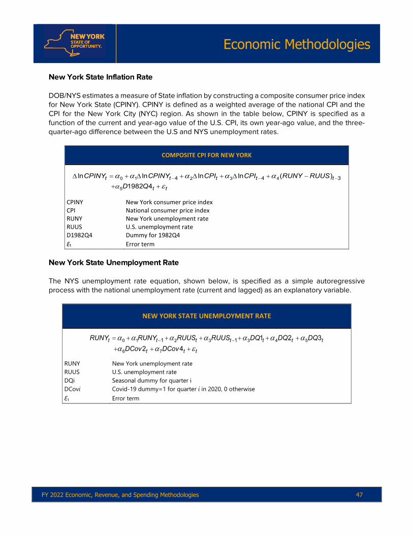
Economic Methodologies
FY 2022 Economic, Revenue, and Spending Methodologies 47
New York State Inflation Rate DOB/NYS estimates a measure of State inflation by constructing a composite consumer price index for New York State (CPINY). CPINY is defined as a weighted average of the national CPI and the CPI for the New York City (NYC) region. As shown in the table below, CPINY is specified as a function of the current and year-ago value of the U.S. CPI, its own year-ago value, and the three-quarter-ago difference between the U.S and NYS unemployment rates.
COMPOSITE CPI FOR NEW YORK
αα α α α α
ε− − −∆ = + ∆ + ∆ + ∆ + −
+ +t t t t t
t t
CPINY CPINY CPI CPI RUNY RUUSD Q
0 1 2 3 4
5
4 4 3ln ln ln ln ( )1982 4
CPINY New York consumer price index CPI National consumer price index RUNY New York unemployment rate RUUS U.S. unemployment rate D1982Q4 Dummy for 1982Q4 Ɛt Error term
New York State Unemployment Rate The NYS unemployment rate equation, shown below, is specified as a simple autoregressive process with the national unemployment rate (current and lagged) as an explanatory variable.
NEW YORK STATE UNEMPLOYMENT RATE
α α α α α α αα α ε
− −= + + + + + +
+ + +t t t t t t t
t t t
RUNY RUNY RUUS RUUS DQ DQ DQDCov DCov
0 1 2 3 3 4 5
6 7
1 1 1 2 32 4
RUNY New York unemployment rate RUUS U.S. unemployment rate DQi Seasonal dummy for quarter i DCovi Covid-19 dummy=1 for quarter i in 2020, 0 otherwise Ɛt Error term

Economic Methodologies
48 FY 2022 Economic, Revenue, and Spending Methodologies
New York State Adjusted Gross Income For estimation work done prior to 2017, DOB used annual sample data on the number of tax returns and the components of New York State adjusted gross income (NYSAGI) created by DTF based on the State’s taxpayer population. The last such sample, for Tax Year 2014, contained 733,702 weighted records and was received in August 2016. In December 2016, DTF began providing a population file; the current version (received in August 2021 and containing tax return data for 2019) contains 10.9 million returns; since this represents all State tax filers, it is no longer weighted. Despite this change in the taxpayer data file, single-equation econometric models are still used to project the number of returns and all the components of taxable income except for the largest component, wages. To ensure consistency with DOB’s New York economic forecast, the forecast growth rate for State wages and salaries derived from DOB/NYS is applied to the wage base obtained from DTF’s taxpayer data. In almost all cases, the NYSAGI components data series are non-stationary. The Division performs a logarithmic transformation which is then first-differenced for all series where at least 26 observations are available, a standard procedure used to avoid spurious regressions. A few shorter series are modeled in levels. DTF attempted to capture as accurately as possible the characteristics of the State taxpayer population in the years when it was constructing the sample. Because it was unreasonable to expect that every component of income would be perfectly represented each year, binary (“dummy”) variables were incorporated into the models where anomalies in the data were thought to be the product of sampling error. Detailed descriptions of the models for the number of returns and for the major components of NYSAGI, other than wages, are presented below. Tax Returns The number of tax returns is expected to vary with the number of households that earn any kind of taxable income during the year. The number of such households, in turn, should be closely associated with the number of individuals who are either self-employed, employed by others, or who earn taxable income from a source other than labor. Total State payroll employment, which is forecast within DOB/NYS, is a key input to this model, because most taxable income is derived from wages and salaries and, thus, is employment related. New Yorkers can earn taxable income from sources other than payroll employment, such as self-employment and real and financial assets. Self-employment is expected to be closely related to proprietors’ income, a component of the NIPA definition of State personal income that is available from BEA and forecast within DOB/NYS. Another component of personal income that is forecast within DOB/NYS, State property income, includes interest, dividend, and rental income. The DOB tax return model shown in the table below incorporates the sum of proprietors’ and property income for New York, deflated by the CPI for New York as constructed by DOB.

Economic Methodologies
FY 2022 Economic, Revenue, and Spending Methodologies 49
Historical data show that a one-time upward shift in the number of tax returns occurred in 1987, thought to be related to the Tax Reform Act of 1986 which was passed by the 99th Congress and signed into law by President Ronald Reagan on October 22, 1986.27 Beginning in 1987, the two-earner deduction for married couples was eliminated, thereby reducing the incentive for married couples to file joint tax returns. To capture this effect, a dummy variable for 1987 is included in the model. A dummy variable for 2000 is included to account for unusual growth in tax returns generated by the stock market.
TAX RETURNS
α α αα α ε+
∆ = + ∆ + ∆ +
+ + t
t t t t t
t t
RET NYSEMP PROPNY YENTNY CPINYD D
0 1 2
3 4
ln ln ln(( ) / )87 00
RET Number of tax returns NYSEMP Total State employment PROPNY State property income YENTNY State proprietors’ income CPINY Consumer Price Index for New York D87 Dummy variable for 1987 tax law change D00 Dummy variable for 2000 stock-market effect Ɛt Error term
Positive Capital Gains Realizations DOB’s positive capital gains realizations forecasting model incorporates those factors that are most likely to influence realization behavior: expected and actual tax law changes; equity market activity; and real estate market activity. Realization behavior appears to exhibit two types of reactions to changes in tax law: a transitory response to an expected change in the law and a permanent response to an actual change. For example, if the tax rate is expected to rise next year, then taxpayers may realize additional gains this year, to take advantage of the lower rate. However, in the long run, the higher tax rate should result in a lower level of current realizations, all things being equal. Based on Miller and Ozanne, the transitory response variable is specified as the square of the difference between the rate expected to take effect next period and the current period rate, with the sign of the difference preserved.28 The long-term or permanent response variable is the actual tax rate. The growth in realizations is expected to be directly related to growth in equity prices. To capture the effect of equity prices, the average price of all stocks traded is incorporated into the model. Forecasts of the average stock price are based on the forecast for the S&P 500 from DOB/U.S.
27 The official citation is P.L. (Public Law) 99-514. 28 Preston Miller and Larry Ozanne, “Forecasting Capital Gains Realizations,” Congressional Budget Office, August 2000.

Economic Methodologies
50 FY 2022 Economic, Revenue, and Spending Methodologies
The average price of stocks traded responds more strongly to declines than to increases in the S&P 500. Fluctuating levels of private equity and hedge fund activity and profitability contribute to capital gains realizations. Private equity firms own stakes in companies that are not listed on a public stock exchange and generally receive a return on their investment through a sale or merger of the company, a recapitalization, or by selling shares back to the public through an IPO. As the table below shows, to capture some of the dynamics of capital gains from private equity funds, the capital gains model includes the value of IPOs. Though small in magnitude, an increase in IPOs is associated with a significant increase in capital gains realizations. The model also contains a measure of real estate market activity, which appears to have grown substantially as a contributor to capital gains realizations since 2000. Taxpayers can exempt gains of up to $250,000 ($500,000 if filing jointly) from the sale of a primary residence, but all other capital gains from real estate transactions are fully taxable. Conditions in the real estate market are captured by including NYS real estate transfer tax (RETT) collections.
POSITIVE CAPITAL GAINS REALIZATIONS
α α α αα α ε
+
+
∆ = ∆ ∆ ∆ ∆
∆
+ +t t t t t
+ +t t t
CG TRSTX PRMTX EQTYP RETT IPO D
1 2 3 4_5 6
ln ln lnln 96 97
CG Positive capital gains realizations
TRSTX Transitory tax measure
PRMTX Permanent tax rate
EQTYP Average price of stocks traded
RETT Real estate transfer tax collections
IPO Value of “true” IPOs
D96_97 Dummy variable, 1 for 1996, -1 for 1997, 0 otherwise Ɛt Error term

Economic Methodologies
FY 2022 Economic, Revenue, and Spending Methodologies 51
Positive Rent, Royalty, Partnership, S Corporation, and Trust Income The largest contributor of New York’s positive partnership, S corporation, rent, royalty, estate and trust gains (PSG) is partnership income, much of which originates in the finance industry. Therefore, growth in PSG is believed to be closely related to overall economic conditions, represented by real U.S. GDP, as well as to the performance of the stock market, represented by the S&P 500. Another large contributor to this AGI category is income from closely held corporations organized under subchapter S of the Internal Revenue Code (“S corporations”). Selection of S corporation status allows firms to pass earnings through to a limited number of shareholders and thus avoid corporate taxation. Empirical work shows that the differential between personal income tax and corporate income tax rates can significantly affect election of S corporation status.29 Personal income increases (other things being constant) as more firms elect S corporation status over C corporation status, which is taxed under the corporate franchise tax. Consequently, DOB’s forecast model for positive partnership, S-corporation, and rent, royalty and trust income, shown below, includes the difference between the corporate franchise tax rate and the maximum marginal personal income tax rate, with the rates being composites of both State and Federal rates. Changes in tax law are believed to account for some of the volatility in PSG. The enactment of the Tax Reform Act of 1986, which created additional incentives to elect S corporation status, likely resulted in an unusually high rate of growth in this income component in the mid- to late 1980s. We observe a particularly high rate of growth in this component in 1988, followed by extremely low growth in 1989. Possible explanations are the expectation of a large tax increase after 1988, or an increase in the fee for electing S corporation status in 1989. This is captured by a dummy variable that assumes a value of one for 1988 and minus one for 1989.
POSITIVE PARTNERSHIP, S-CORPORATION, RENT, ROYALTY, ESTATE AND TRUST INCOME
α α α α α ε∆ = + ∆ + ∆ + ∆ + +t t t t t tPSG MTR SP GDP D 0 1 2 3 4ln ln ln 88 _ 89
PSG Partnership, S-corporation, rent, royalty, estate and trust income
MTR Difference between corporate and personal income maximum marginal tax rates SP Standard and Poor’s 500 stock index GDP Real U.S. GDP D88_89 Dummy variable, 1 for 1988, -1 for 1989, 0 otherwise Ɛt Error term
29 See, for example, Robert Carroll and David Joulfaian, “Taxes and Corporate Choice of Organizational Form,” OTA Paper 73, Office of Tax Analysis, U.S. Treasury Department, Washington, DC, October 1997.

Economic Methodologies
52 FY 2022 Economic, Revenue, and Spending Methodologies
Dividend Income Dividend income is linked to the fortunes of publicly held U.S. firms, which, in turn, are expected to vary with the business cycle. The inclusion of U.S. dividend income serves as a proxy for the profitability of publicly held U.S. firms and ensures consistency with DOB’s macroeconomic forecast model. Dividend income is also thought to be associated with firms’ expectations pertaining to their future profitability, which should be tied to the future strength of the economy. Equity market prices, a leading economic indicator, should vary with expected future dividend payouts and thus enters the specification shown below. Because interest rates incorporate inflation expectations, which in turn contain expectations regarding the future strength of the economy, they also represent a proxy for the latter. Interest rates are represented by the rate on the 10-year Treasury yield. Historically, changes in State dividend income have ranged from a decrease of 29 percent in calendar year 2009 to an increase of 27 percent in 2004, indicating that it is much more variable than dividend income on the national level. This may suggest the importance of factors affecting the way taxpayers report their income, rather than changes in the payment of dividends by firms. The Tax Reform Act of 1986 lowered the maximum tax rate on dividend income for New York taxpayers from 64 percent in 1986 to 36 percent in 1988. A dummy variable is included to control for what is assumed to be the impact of this Act on the reporting of taxable dividend income. Another dummy variable captures the impact of recessions (1975, 1990, 1991, 1992, 2001, 2002, 2008, and 2009).
DIVIDEND INCOME
α α α α αα ε
+
+
∆ = ∆ + ∆ + ∆ +
+t t t t t t
t t
DIV USDIV TRATE SP DREC D _D
1 2 3 4 5
6
ln ln 10 ln 88 8905
DIV Dividend income USDIV US dividend income under NIPA TRATE10 10-year Treasury yield SP Standard and Poor’s 500 stock Index DREC Recession dummy variable D88_89 Dummy variable, 1 for 1988, -1 for 1989 D05 Dummy variable = 1 for 2005, 0 otherwise Ɛt Error term
Interest Income For a given amount of assets, an increase in interest rates will increase interest income. DOB’s forecasting model for interest income is based on this simple concept and so includes the U.S. federal funds interest rate. In addition, the overall trend in taxable interest income for New York

Economic Methodologies
FY 2022 Economic, Revenue, and Spending Methodologies 53
has been found to track New York property income, a component of State personal income that combines interest, dividend, and rental income. The model specification that follows further includes a dummy variable to capture the impact of recessions (1975, 1990, 1991, 1992, 2001, 2002, 2008, and 2009) on interest income.
INTEREST INCOME
α α ε+ +∆ =α ∆ + ∆t t t t tINT FFRATE PROPNY DREC1 2 3ln ln
INT Interest income FFRATE Federal funds rate PROPNY New York property income DREC Recession dummy variable Ɛt Error term
Business Income Business income combines income earned and reported due to operating a business, or practicing a profession as a sole proprietor, or from farming. Business income is expected to vary with the overall strength of the State and national economies. The inclusion in the model of State proprietors’ income, a component of the NIPA definition of New York personal income, which is forecast within DOB/NYS, insures consistency between DOB’s New York forecast and the forecast of this NYSAGI component.
BUSINESS INCOME
α α α ε+ +∆ = ∆ + ∆ tt t t tBUS YENTNY GDP D 1 2 3ln ln ln 89
BUS Sole proprietor and farm income YENTNY State proprietor income (NIPA definition) GDP Real U.S. GDP D89 Dummy variable for 1989 onward Ɛt Error term
The impact of the national business cycle is captured using real GDP, which is forecasted in DOB/US In addition, a dummy variable is included to capture the downward shift in reported business income growth for the period from 1989 onward, perhaps due to new firms registering as S corporations rather than sole proprietorships, thus taking advantage of more favorable tax laws. The model specification is shown above.
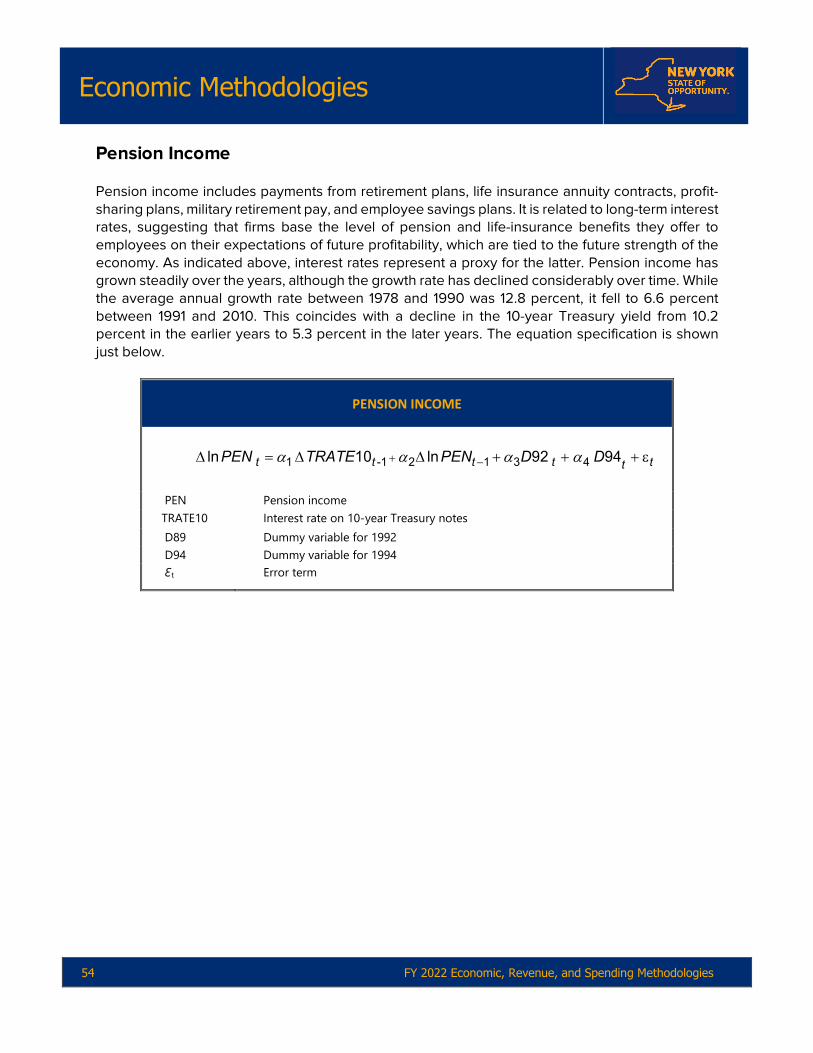
Economic Methodologies
54 FY 2022 Economic, Revenue, and Spending Methodologies
Pension Income Pension income includes payments from retirement plans, life insurance annuity contracts, profit-sharing plans, military retirement pay, and employee savings plans. It is related to long-term interest rates, suggesting that firms base the level of pension and life-insurance benefits they offer to employees on their expectations of future profitability, which are tied to the future strength of the economy. As indicated above, interest rates represent a proxy for the latter. Pension income has grown steadily over the years, although the growth rate has declined considerably over time. While the average annual growth rate between 1978 and 1990 was 12.8 percent, it fell to 6.6 percent between 1991 and 2010. This coincides with a decline in the 10-year Treasury yield from 10.2 percent in the earlier years to 5.3 percent in the later years. The equation specification is shown just below.
PENSION INCOME
α α α α+ −∆ = ∆ ∆ + + + εt t t t ttPEN TRATE PEN D D1 -1 2 1 3 4ln 10 ln 92 94
PEN Pension income TRATE10 Interest rate on 10-year Treasury notes D89 Dummy variable for 1992 D94 Dummy variable for 1994 Ɛt Error term
Part II:
Revenue Methodologies

Revenue Methodologies
56 FY 2022 Economic, Revenue, and Spending Methodologies
Alcoholic Beverage Taxes Forecast Methodology The alcoholic beverage tax forecast is primarily based on an analysis of historical alcoholic beverage consumption trends. Two growth rates used to analyze and help project future cash receipts are:
• trend growth rate which quantifies the rate of growth over a specified time period; and
• compound annual growth rate which is the uniform growth rate required each year over a specified time period to grow the series from the starting to the ending amount. The time period analyzed includes historical collections data, but more significance is given to recent (i.e., prior five years) collections trends.
Final estimates are constructed using the growth rate-based forecasts with possible adjustments made for audits, refunds, credits, enforcement issues, pay schedule lags, accounting delays, historical and year-to-date collection patterns, and tax policy and administrative changes. Risks to the Forecast The receipts forecast includes risks such as:
• Unpredictable changes in consumption behavior that influence collections; and
• The depletion or replenishment of inventories at the wholesale level.

Revenue Methodologies
FY 2022 Economic, Revenue, and Spending Methodologies 57
Cigarette and Tobacco Taxes Forecast Methodology Cigarette Excise Tax The estimation process for the cigarette excise tax is as follows:
1. Logarithmic transformation of the monthly cigarette tax stamp sales data series;
2. The resulting series serves as the dependent variable ln(STAMPSALES) in the model described below.
a. All variables in the model are monthly with the real price in logarithmic form. We adjust for seasonality via the use of dummies (March is omitted to maintain the intercept term). Note that the estimated coefficients for the trend and the logarithm of the real price without tax variables must be compounded over 12 months to be annualized (e.g., the estimated trend decline in stamp sales, all else equal, is approximately four percent annually).
= - -
- + + U t
TAXABLE CIGARETTE CONSUMPTION MODEL
ln(STAMPSALES) t Constant TREND t ln(REAL PRICE) t
Note: U t = Residual
PRE BUYTAX RATE t
ln(STAMPSALES): the logarithm of purchases of cigarettes tax stamps in NYS. TREND: a time-series estimation technique that employs a numeric variable synonymous with the observation (i.e., at observation1, Time = 1; at observation2, Time = 2, etc.). This effectively is a substitute for a non-observable variable that both affects the dependent variable and is substantially correlated with time. ln(REAL PRICE): the logarithm of the average monthly price, excluding State tax, of cigarettes in NYS.30 This is indexed to 1982-84 and divided by the CPI to measure the price of cigarettes relative to the overall prevailing price level. TAX RATE: the State cigarette tax rate expressed in cents per pack.
30 As reported in The Tax Burden on Tobacco, Orzechowski and Walker, Volume 54, 2019.
Revenue Methodologies
58 FY 2022 Economic, Revenue, and Spending Methodologies
PRE BUY: dummy variable equal to 1 in the month prior to a State tax increase, -1 in the month following a State tax increase and zero in all other months to capture the impacts of pre-buying on stamp sales.
3. After generating cigarette stamp sales annual growth rates and applying them to stamp sales revenue, audit and refund estimates are added into the series to arrive at estimates for cash collections. Adjustments are often made based on historical and year-to-date collection patterns as suspected tax evasion routinely causes collections to be lower than estimated model results, especially with NYC stamp sales revenue where there is an additional $1.50 per pack excise tax imposed. Other adjustments may be made for refunds, credits, pay schedule lags, accounting delays, tax law and administrative changes, and the estimated impact of discrete events, such as large price increases by manufacturers, Federal and State cigarette excise tax changes, and enforcement efforts on cigarette tax revenues.
Tobacco Products Tax Tobacco products tax receipts are a small component of the cigarette and tobacco taxes (approximately eight percent). This tax is imposed on products such as cigars, pipe tobacco and chewing tobacco. Trend analysis is used to construct a tobacco products tax forecast, with greater significance given to recent trends (i.e., the prior five years). Risks to the Forecast The receipts forecast includes risks such as:
• Increases in the price of cigarettes, primarily from tax increases;
• Unanticipated changes in the consumer responsiveness to future price/tax changes;
• Price changes in nearby states that could increase or lessen the incentive for consumers to evade the tax; and
• The effects of the Cigarette Strike Force unit within the DTF’s Criminal Investigations
Division.
Revenue Methodologies
FY 2022 Economic, Revenue, and Spending Methodologies 59
Corporation Franchise Tax Forecast Methodology Current year and outyear estimates of CFT are based on a combination of historical collection patterns, trending techniques, estimates of underlying taxpayer liability, and a microsimulation model that incorporates statutory changes. Current Year Forecast The current year estimation process involves the following steps:
1. Analyze historical trends in the components of cash collections by comparing year-to-date payments to historical averages for the same portion of the fiscal year to estimate remaining receipts for the year;
2. Adjust for collection abnormalities caused by administrative and tax law changes and
economic shocks that may disrupt otherwise stable patterns observable over several years;
3. Track liability payment streams for calendar year and fiscal year filers (current year, prior year adjustments and the prepayment on next year’s liability) and the other unassigned liability payments (other payments, audit and compliance receipts and Article 13 receipts) to arrive at estimates of current SFY collections; and
4. Review the tracking and estimation of audit and compliance receipts. Receipts from the Metropolitan Transportation Authority (MTA) surcharge are estimated in the current year using the same historical ratio analysis employed to estimate General Fund receipts with audit and compliance receipts estimated separately.
Outyear Forecast The outyear estimation process involves the following steps:
1. Derive annual growth rates for the three tax bases:
a. The aggregate business income base is trended using U.S. corporate profits; industry profits outlook and anecdotal information on industrial sectors are also examined to monitor trends that could specifically impact tax receipts;
b. The asset base is trended using U.S. investment in equipment and software. This variable is highly correlated with the total asset variable used to calculate the capital base tax, which is 0.1875 percent for tax years 2021 to 2023 and 0 percent thereafter; and
c. U.S. CPI is used to trend the fixed dollar minimum tax base variable, which represents less than two percent of total tax liability.

Revenue Methodologies
60 FY 2022 Economic, Revenue, and Spending Methodologies
2. Use the growth rates derived from Step (1) to trend Tax Year liability in a microsimulation model based on the actual calculation of tax due in each tax year based on current law. The model calculates liability for taxpayers that is used to produce a baseline estimate for gross receipts. Liability is simulated from the base for past years as well as the outyear forecast. The growth rates used in the trending for the current forecast are shown below.
0.0%
1.0%
2.0%
3.0%
4.0%
5.0%
(10%)
(5%)
0%
5%
10%
15%
20%
25%
2018 2019 2020 2021 2022 2023 2024 2025
Percent (U.S. CPI)
Economic Variables Year-Over-Year Percent Change
U.S. Corporate Profits U.S. Investment in Equipment and Software U.S. CPI
Perc
ent (
U.S.
Cor
pora
te P
rofit
s; U.
S.
Inve
stm
ent i
n Eq
uipm
ent a
nd S
oftw
are)
3. Sum results from the CFT microsimulation model to produce the CFT payment estimates for each forecast year;
4. Make out-of-model adjustments for the estimated impact of tax law changes (e.g.,
non-refundable tax credits), current year cash receipts and any administrative actions. As additional information from recent quarterly payments, tax returns or other sources becomes available, revisions to the estimated impact of significant tax law changes and current year cash receipts can produce substantial revisions to the net receipts estimate;
5. Based on historical trends, adjust for the incremental impact of the larger refundable tax
credits. This approach allows for the incorporation of recent refund activity while ensuring that the historical level of refunds is considered along with recently created or enhanced tax credits. Credit refund claims are paid at the conclusion of the audit review process, which is unique for each case and can skew the percentage distribution of net receipts when they are paid;

Revenue Methodologies
FY 2022 Economic, Revenue, and Spending Methodologies 61
6. Add estimates for audit and compliance receipts to the baseline estimate for gross receipts to arrive at a baseline, net receipts cash estimate; and
7. Outyear MTA surcharge estimates are generated by multiplying the ratio of non-audit General Fund receipts to non-audit MTA surcharge receipts.
Risks to the Forecast The receipts forecast includes risks such as:
• The volatile relationship between liability and the underlying economic factors, as well as difficulty in estimating the SFY in which cash receipts from that liability will be received. These relationships can be greatly altered by numerous factors through time;
• Audit and compliance results;
• Estimated impacts of tax law changes introduce additional risk from a variety of sources
(initial estimate, timing issues related to taxpayer awareness, and voluntary compliance); and
• Changes in the relationship between corporate profits and tax liability and errors in the
forecast of corporate profits provide additional risk to the CFT estimate.

Revenue Methodologies
62 FY 2022 Economic, Revenue, and Spending Methodologies
Corporation and Utilities Tax Forecast Methodology Current year and outyear estimates for public utility companies are based on a combination of historical collection patterns, simple trending techniques, and statutory changes or other unexpected occurrences that may affect collections. Current Year Forecast The current year estimation process involves the following steps:
1. Analyze historical trends in the components of cash collections by comparing year-to-date payments to historical averages for the same portion of the fiscal year to estimate remaining receipts for the year; and
2. Review the tracking and estimation of audit and compliance receipts. Outyear Forecast The outyear estimation process involves the following steps:
1. Apply multi-year, historical average growth rates in gross receipts to the current year liability;
2. Translate liability estimates to SFY cash receipts, which are then adjusted to reflect the estimated effects of law changes and other non-economic factors that affect collections; and
3. Add estimates for audit and compliance receipts to the baseline estimate for gross receipts to arrive at a baseline, net receipts cash estimate.
Telecommunication Companies The growth rate of telecommunication revenue is kept at an annual two percent decline during the forecast period due to the increase in use of internet-based communications (which are not taxable) and the competitive nature of the industry (which can change the taxable base). Risks to the Forecast The receipts forecast includes risks such as:
• Uncertainty related to energy prices, changes in supply and demand, business market conditions, changes in technology and general inflation;

Revenue Methodologies
FY 2022 Economic, Revenue, and Spending Methodologies 63
• Future statutory, regulatory, and administrative changes, including Federal Tax Law changes that affect tax rates and bases;
• Changes and trends in residential energy consumption; and
• Future trends in the wireless telecommunication industry.
Revenue Methodologies
64 FY 2022 Economic, Revenue, and Spending Methodologies
Employer Compensation Expense Tax Forecast Methodology The Employer Compensation Expense Tax (ECET) estimation process involves the following steps:
1. Grow the most recently completed monthly collections totals by the corresponding quarterly wage growth forecast.
• A lack of long-term historical collections data necessitates dependency on a small set of data points.
2. Proportionally adjust the projected collection series to reflect the initial three-year tax rate
phase-in. This rate increased from 1.5% in Tax Year 2019 to 3.0% (Tax Year 2020) and then 5.0% (Tax Years 2021 and after).
3. Proportionally adjust the projected collection series for projected growth in eligible
employer participation.
4. Aggregate the resulting monthly totals into fiscal year forecasts. Risks to the Forecast The receipts forecast includes risks such as:
• Errors from referencing the most recent historical collections data, including processing distortions that may not be repeated;
• Uncertainty related to the participation growth rate of eligible employers;
• Wage forecast errors;
• Errors related to the application of an aggregate quarterly wage forecast to a relatively
small subset of employers;
• Uncertainty regarding the share of total wages in excess of $40,000 per employee (wages below $40,000 are not subject to tax); and
• Unanticipated Federal administrative or legislative action to limit the value of the Employer Compensation Expense Tax.
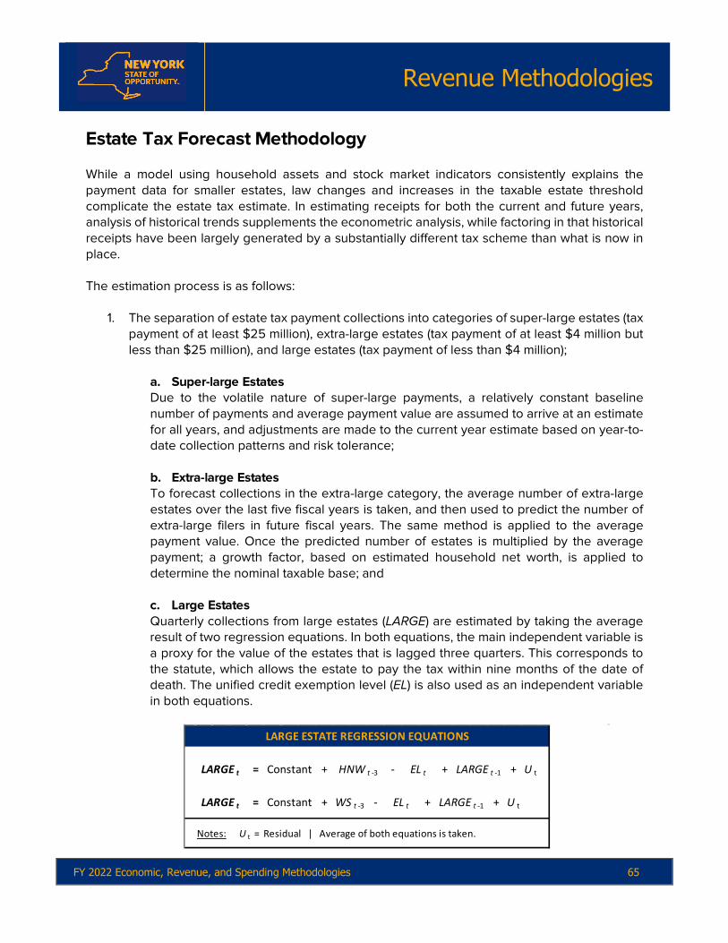
Revenue Methodologies
FY 2022 Economic, Revenue, and Spending Methodologies 65
Estate Tax Forecast Methodology While a model using household assets and stock market indicators consistently explains the payment data for smaller estates, law changes and increases in the taxable estate threshold complicate the estate tax estimate. In estimating receipts for both the current and future years, analysis of historical trends supplements the econometric analysis, while factoring in that historical receipts have been largely generated by a substantially different tax scheme than what is now in place. The estimation process is as follows:
1. The separation of estate tax payment collections into categories of super-large estates (tax payment of at least $25 million), extra-large estates (tax payment of at least $4 million but less than $25 million), and large estates (tax payment of less than $4 million);
a. Super-large Estates Due to the volatile nature of super-large payments, a relatively constant baseline number of payments and average payment value are assumed to arrive at an estimate for all years, and adjustments are made to the current year estimate based on year-to-date collection patterns and risk tolerance;
b. Extra-large Estates To forecast collections in the extra-large category, the average number of extra-large estates over the last five fiscal years is taken, and then used to predict the number of extra-large filers in future fiscal years. The same method is applied to the average payment value. Once the predicted number of estates is multiplied by the average payment; a growth factor, based on estimated household net worth, is applied to determine the nominal taxable base; and
c. Large Estates Quarterly collections from large estates (LARGE) are estimated by taking the average result of two regression equations. In both equations, the main independent variable is a proxy for the value of the estates that is lagged three quarters. This corresponds to the statute, which allows the estate to pay the tax within nine months of the date of death. The unified credit exemption level (EL) is also used as an independent variable in both equations.
= + - + + U t
= + - + + U tEL t LARGE t -1
Notes: U t = Residual | Average of both equations is taken.
LARGE ESTATE REGRESSION EQUATIONS
LARGE t Constant HNW t -3 EL t LARGE t -1
LARGE t Constant WS t -3

Revenue Methodologies
66 FY 2022 Economic, Revenue, and Spending Methodologies
HNW: household net worth as a function of financial assets and nominal home prices.
EL: the unified credit exemption level. Values after the 3rd quarter of 2014 include the phase-in of the higher filing threshold.
WS: the Wilshire 5000 equities index, used as a proxy to capture the contribution of equity markets to the taxable estate.
HV: the average value of a single-family home in NYS.
2. The estimates from each estate category are added together, along with audit and refund
estimates for each fiscal year, to arrive at total estate tax receipts forecasts; and
3. Final adjustments are regularly made based on year-to-date collections and from a risk assessment perspective due to the highly volatile nature of this tax.
Risks to the Forecast Risks to the receipts forecast include:
• Errors in the exogenous variable forecasts;
• The inherent difficulty of forecasting the tax liability of a decedent’s estate; and
• The inherent difficulty of estimating the impact of significant tax law changes.

Revenue Methodologies
FY 2022 Economic, Revenue, and Spending Methodologies 67
Fuel Taxes Forecast Methodology Fuel taxes consist of the motor fuel tax (MFT) and the petroleum business tax (PBT). The estimation process is as follows:
1. Produce an annual forecast of demand (taxable gallons of fuel consumed) from fiscal year data. Gasoline consumption growth is taken from the average of two different approaches:
a. The first approach uses the Energy Information Administration (EIA) estimated
relationships between changes in real GDP, national fuel prices, and national gasoline demand. EIA estimates that a one percent increase in real GDP will raise gasoline demand by 0.1 percent, and a 10 percent increase in fuel prices will decrease demand by 0.3 percent. To derive a State level forecast, real NYS disposable income growth is substituted for GDP.
Real NYS NYSDisposable
IncomeGasoline
Price
FY 2012 0.5% 24.3%FY 2013 3.0% 1.8%FY 2014 -1.5% -4.7%FY 2015 2.8% -10.9%FY 2016 3.7% -25.8%FY 2017 3.2% -1.6%FY 2018 4.6% 10.7%FY 2019 1.9% 6.8%FY 2020 1.7% -3.5%FY 2021 7.1% -13.6%
PERCENT CHANGE IN EXOGENOUS VARIABLES
b. The second approach uses the gasoline demand growth from the most recent EIA Annual Energy Outlook report.
The estimate of automotive diesel consumption for fuel taxes is derived by using the diesel demand growth from the most recent EIA Annual Energy Outlook. However, since this is an annual report, adjustments are made throughout the forecast period if there are significant changes to real GDP. In addition, a trend growth rate is used for comparison purposes to the EIA estimated demand growth rate to determine if economic activity has changed since the release of the annual report. PBT is also imposed on several other non-automotive fuel types (distillate, residual, kero-jet, aviation gasoline, railroad diesel, etc.). Receipts from these fuel types are roughly two
Revenue Methodologies
68 FY 2022 Economic, Revenue, and Spending Methodologies
percent of total PBT receipts. For these other fuel types, recent trend growth rates are typically used to generate demand forecasts.
2. Apply appropriate tax rates to the estimates of taxable gallonage. Specific to PBT only, the
base and supplemental tax rates are indexed with annual adjustments made on January 1 to reflect the percent change in the Producer Price Index (PPI) for refined petroleum products for the 12 months ending August 31 of the preceding year. Tax rates cannot increase or decrease by more than five percent per year. DOB forecasts the PPI used for indexing based on historical data.
3. Make various adjustments to arrive at the forecast of cash collections, since a direct relationship does not exist between reported gallonage and cash collections. Adjustments may be made for refunds, credits, pay schedule lags, accounting delays, historical and year-to-date collection patterns, and tax law and administrative changes.
Risks to the Forecast The receipts forecast includes risk such as unexpected variation in fuel prices due to changes in global economic and political conditions. Fuel price changes in turn impact fuel consumption, fuel inventories, tax evasion, and the PBT rate index.

Revenue Methodologies
FY 2022 Economic, Revenue, and Spending Methodologies 69
Gaming Forecast Methodology Video Lottery Terminals (VLTs) The forecast for VLT receipts is primarily based on an analysis of recent trends (i.e., prior five years in the net machine income (NMI) of each VLT facility. This analysis is supplemented by the estimated impacts of discrete events such as: a significant change in the number of machines; a major renovation or change in amenities; a shock to the economy; or a notable change by a nearby competing gaming facility. Once final NMI estimates are generated for each VLT facility, the statutory aid to education rates are applied. The Gaming Commission receives a share of NMI as an administrative allowance to cover administrative expenses. A portion of the unused administrative allowance is directed to aid to education at the end of the fiscal year. This administrative surplus estimate is made in conjunction with the Gaming Commission based on the initial NMI estimates and the Commission’s expected administrative expenses. Additional commission estimate amounts are provided for certain facilities out of Video Lottery Gaming (VLG) aid to education revenue. These figures are based upon NMI totals from the prior fiscal year. Each of these different aid to education revenue sources are summed to arrive at a total VLT receipts estimate. Adjustments may be made for accounting delays, minor non-recurring revenue sources, historical and year-to-date collection patterns, and law and administrative changes. Commercial Gaming The forecast for commercial gaming is primarily based on analysis of recent trends of the slot and table game (including sports wagering) gross gaming revenue (GGR) of each gaming facility. Specifically, year-to-date collections patterns are given significant importance due to the lack of historical observations. This analysis is supplemented by the estimated impacts of discrete events such as: a significant change in the number of machines and/or table games; a major renovation or change in amenities; a shock to the economy; or a notable change by a nearby competing gaming facility.
Once final slot and table game GGR estimates are generated for each gaming facility, the statutory tax rates are applied. Adjustments may be made for accounting delays, significant changes in free play offered, and law and administrative changes. Traditional Lottery Cash sales for the various lottery games are initially estimated using analysis of both historical and recent trends; and adjustments are subsequently made for the estimated impacts of marketing, operational, and promotional plans, new game introductions, and various other discrete events as noted below.

Revenue Methodologies
70 FY 2022 Economic, Revenue, and Spending Methodologies
Instant Cash Games Instant Cash game sales are forecasted using trend analysis with adjustments typically made for marketing and operational plans. As the prize payout and education amount generated is dependent on the two types of instant games sold (64.25 percent and 74.25 percent payout games), it is important to accurately forecast the split in sales. Analysis requires careful consideration of the timeline of marketing and promotional efforts, the timing of the introduction of new scratch-off games throughout the year and the seasonality of sales. Draw Games Sales of Mega Millions and Powerball tickets are volatile because the game jackpots can “roll-up” to high amounts. High jackpots produce significant sales spikes. The forecast of these games is inherently risky because it requires an assumption of the number and level of “roll-ups” expected to occur in a given State Fiscal Year. Analysis requires careful consideration of historical sales-to-jackpot relationships, seasonal effects, and other factors such as “jackpot fatigue” (i.e., the diminishing sales associated with a particular jackpot level over time) and the coverage ratio (the combinations actually bet, divided by the total number of combinations). These games can also be impacted by policy changes or other events such as changing the size of the matrix, changing the price of the game, and altering the jackpot structure. Sales for the rest of these games are generally estimated using trend analysis, with a focus on trends of the last five years. Analysis requires careful consideration of seasonality of sales, the number of draws per day, marketing and promotional efforts, and any other game-specific factors, changes, or events. Sales of these games have proven to be much more stable compared to the large jackpot games. Like the administrative allowance for VLTs, a portion of lottery game sales are directed to the Gaming Commission to cover administrative expenses. The same administrative surplus estimate process as described for VLTs also applies to traditional lottery games. After generating the sales forecasts and applying statutory aid to education rates and adding the administrative surplus estimate, adjustments may be made for accounting delays, historical and year-to-date collection patterns, and law and administrative changes. Interactive Fantasy Sports (IFS) The forecast for IFS is primarily based on an analysis of recent IFS consumption trends and NYS’s resident percentage. Trend analysis is used to determine growth rates for IFS handle (IFS contest entry fees) and NYS’s resident percentage, which are then separately applied to base year IFS handle and NYS resident percentage. Those two figures are multiplied to arrive at NYS handle. The tax rates are then applied to the estimate of NYS handle to arrive at an IFS tax revenue estimate.

Revenue Methodologies
FY 2022 Economic, Revenue, and Spending Methodologies 71
After generating a growth-rate based forecast, adjustments are made for historical and year-to-date collection patterns and law and administrative changes. Risks to Forecast The VLT and commercial gaming receipts forecast includes risks such as:
• Economic constraints experienced by consumers;
• Competition and expansion from commercial gaming facilities in NYS (as they progress towards stable operations), Native American casinos, and casinos in neighboring states;
• Future law or administrative changes;
• Significant changes in marketing or promotional strategies; and
• Facility closures or capacity restrictions. The traditional lottery receipts forecast includes risks such as:
• Economic constraints experienced by consumers;
• Mega Millions and Powerball games achieving lower or higher than forecasted sales if the number or level of large jackpots deviates more than expected;
• Significant shifts in sales in a certain type of game that may reduce sales from a similar,
competing game type, potentially impacting aid to education receipts depending on the aid to education rates of such games; and
• Competition from other gaming options that may also reduce lottery sales.
The IFS receipts forecast includes risks such as:
• Economic constraints experienced by consumers; and .
• Cancellation or suspension of sports leagues.

Revenue Methodologies
72 FY 2022 Economic, Revenue, and Spending Methodologies
Highway Use Tax Forecast Methodology The Highway Use Tax (HUT) is composed of the following three components: Truck Mileage Tax (TMT) The forecast is primarily based on analysis of recent TMT trends, with two growth rates used to analyze and project future cash receipts. The trend growth rate quantifies the rate of growth over a specified time period. The compound annual growth rate is the uniform growth rate required each year over a specified time period to grow the series from the starting to the ending amount. The time period being analyzed includes historical collections, but more significance is given to recent (i.e., prior five years) collections trends. Final estimates are constructed using the growth rate-based forecasts with possible adjustments for audits, refunds, enforcement issues, year-to-date collection patterns, as well as tax policy and administrative changes. Fuel Use Tax (FUT) The diesel forecast, detailed in the Fuel Taxes section of this volume, is used as a proxy for FUT collections. Adjustments may be made for audits, refunds, enforcement issues, year-to-date collection patterns, as well as tax policy and administrative changes. Registration Fees Like the TMT forecast, historical trends are used to estimate the amount of revenue collected from registration fees, along with any necessary adjustments. Recent adjustments reflected:
• the registration fee’s reduction to $1.50 with the FY 2017 Enacted Budget - down from a $15 registration fee coupled with a $4 decal fee; and
• a FY 2019 adjustment to reflect a reclassification of registration monies to the TMT.
Risks to Forecast The receipts forecast is dependent upon the demand for trucking, which fluctuates with national and NYS economic conditions. Specifically, FUT collections fluctuate with fuel consumption, which is influenced by both economic conditions and fuel prices. Furthermore, fuel prices also affect FUT collections by dictating whether a driver chooses to purchase fuel in-State or out-of-State in certain regions. When drivers purchase fuel out-of-State, but use it in-State, fuel use tax collections increase, while motor fuel tax and sales tax collections both decrease.
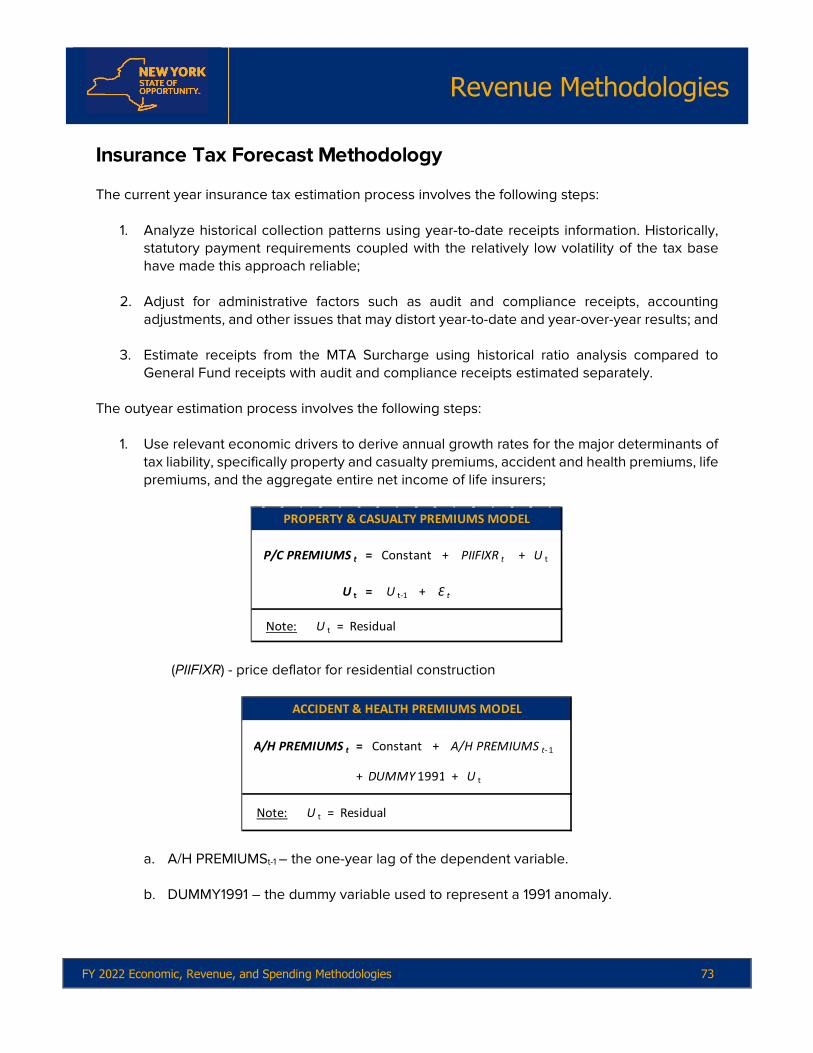
Revenue Methodologies
FY 2022 Economic, Revenue, and Spending Methodologies 73
Insurance Tax Forecast Methodology The current year insurance tax estimation process involves the following steps:
1. Analyze historical collection patterns using year-to-date receipts information. Historically, statutory payment requirements coupled with the relatively low volatility of the tax base have made this approach reliable;
2. Adjust for administrative factors such as audit and compliance receipts, accounting adjustments, and other issues that may distort year-to-date and year-over-year results; and
3. Estimate receipts from the MTA Surcharge using historical ratio analysis compared to General Fund receipts with audit and compliance receipts estimated separately.
The outyear estimation process involves the following steps:
1. Use relevant economic drivers to derive annual growth rates for the major determinants of tax liability, specifically property and casualty premiums, accident and health premiums, life premiums, and the aggregate entire net income of life insurers;
= + + U t
U t = + Ɛ tU t-1
Note: U t = Residual
PROPERTY & CASUALTY PREMIUMS MODEL
P/C PREMIUMS t Constant PIIFIXR t
(PIIFIXR) - price deflator for residential construction
= +
+ + U t
A/H PREMIUMS t- 1ConstantA/H PREMIUMS t
DUMMY 1991
ACCIDENT & HEALTH PREMIUMS MODEL
Note: U t = Residual
a. A/H PREMIUMSt-1 – the one-year lag of the dependent variable.
b. DUMMY1991 – the dummy variable used to represent a 1991 anomaly.

Revenue Methodologies
74 FY 2022 Economic, Revenue, and Spending Methodologies
= + + U t
Note: U t = Residual
TIME tConstantLIFE PREMIUMS t
LIFE PREMIUMS MODEL
TIME – a simple time trend.
= + +
Note: U t = Residual
EARNED NET INCOME LIFE MODEL
ConstantENILIFE t Z t U t
Z – a measurement of U.S. corporate profits.
2. Use the growth rates from (1) to trend tax year liability in a microsimulation model based on the actual calculation of tax due in each tax year;
2013 2014 2015 2016 2017 2018 2019 2020Lines of Insurance
Automobile 13,074.0 13,583.6 14,145.1 15,004.4 15,875.5 16,635.1 17,045.1 16,802.1percent change 3.5 3.9 4.1 6.1 5.8 4.8 2.5 (1.4)Worker's Compensation 5,191.5 5,261.1 5,523.6 5,893.9 5,942.5 5,917.7 5,620.6 4,749.9percent change 9.2 1.3 5.0 6.7 0.8 (0.4) (5.0) (15.5)Commercial Multi-Peril 3,487.5 3,613.5 3,591.8 3,659.4 3,863.0 3,958.4 4,097.3 4,119.1percent change 7.3 3.6 (0.6) 1.9 5.6 2.5 3.5 0.5General Liability 4,977.7 5,313.7 5,709.7 5,829.8 5,646.7 6,092.6 6,759.6 7,259.3percent change 11.5 6.8 7.5 2.1 (3.1) 7.9 10.9 7.4Homeowner's Multi-Peril 4,901.5 5,085.5 5,195.8 5,224.1 5,286.0 5,396.8 5,593.1 5,815.5percent change 4.2 3.8 2.2 0.5 1.2 2.1 3.6 4.0Other 6,373.1 6,436.3 6,391.7 6,380.8 6,294.5 6,628.0 6,750.9 6,809.3percent change 3.9 1.0 (0.7) (0.2) (1.4) 5.3 1.9 0.9TOTAL P/C PREMIUMS 38,005.2 39,293.8 40,557.8 41,992.5 42,908.3 44,628.7 45,866.8 45,555.2percent change 5.7 3.4 3.2 3.5 2.2 4.0 2.8 (0.7)
NEW YORK CALENDAR YEARPROPERTY AND CASUALTY INSURANCE PREMIUMS
(millions of dollars/percent)
Source: New York State Department of Financial Services and the NAIC's I-site after 2012.
3. Compare simulated liability from past years to actual liability payments to adjust results where appropriate;
4. Make additional adjustments for the estimated impact of law changes;

Revenue Methodologies
FY 2022 Economic, Revenue, and Spending Methodologies 75
5. Translate adjusted current year payment estimates to SFY cash estimates using historical relationships between current year payments and other payments (pre-payments, prior year adjustments, etc.); and
6. Adjust for audit and compliance receipts recovered by DTF, and tax collections received
by the Department of Financial Services (DFS). Risks to the Forecast The receipts forecast includes risk such as:
• Unexpected changes in premiums caused by changes in underwriting practices, surplus and reserves, regulations, and unexpected catastrophes;
• Changes in consumer behavior as it relates to the purchase of coverage for property and
casualty insurance policies. Significant changes in the economy may result in consumers changing their level of property and casualty insurance coverage; and
• National and state trends on health care premiums.

Revenue Methodologies
76 FY 2022 Economic, Revenue, and Spending Methodologies
Personal Income Tax Forecast Methodology The personal income tax (PIT) estimating/forecasting process has three major steps performed as follows:
1. NYSAGI (NYS adjusted gross income) forecasting uses a set of single-equation econometric models to project the separate components of gross taxable income. Here, the historical files are used to create a database of the NYSAGI income components. The NYSAGI models use this information, together with historical data and forecasts from DOB’s U.S. and NYS models, to make forecasts of the NYSAGI income components. Given the lag with which actual tax return data are available, results from these models are often adjusted to reflect the latest cash information. For further information on this process, please see the “New York State Adjusted Gross Income” chapter of this Volume.
2. PIT liability forecasting combines results from the NYSAGI models with the population file
data to forecast PIT liability. It can also be used to assess the impact of tax law changes. Computing liability beyond the base year adds an additional step to the process. First, taxpayer incomes are trended forward by growing the individual income components by adjusting the weights created after the population file’s base year to reflect the results from the NYSAGI models. Second, liability is calculated.
The process of trending taxpayer incomes to calculate liability is done sequentially as the latest population data forms the base for the next year’s “trended” dataset, which in turn becomes the base for creating the subsequent trended dataset, and so on. Once created, the new “trended” datasets can be submitted to the second step, the computation of tax liability, given taxpayers’ trended incomes and existing tax law for that year.
Note that because study files beginning with the 2015 tax year contain the entire population of filers, a necessary preliminary step is to use certain population characteristics to create weights so that the trending process’s loss-minimization function can work. Prior to the 2015 tax year, the study files were largely (though not entirely) stratified random samples and so were weighted by DTF.
a. An initial stage of the trending process takes the aggregate growth rates of the six
largest AGI components for residents - wages and salaries, positive capital gains realizations, positive partnership and S corporation gains, dividend income, interest income, proprietors and farm income, as well as nonresident wages and salaries – and allows their growth rates to vary by income. These growth rates are determined by a set of econometric models that forecast the shares of the major components by income deciles. These shares are constrained to add to unity, ensuring that the aggregate income targets are met. Income deciles are determined based on the taxpayer’s NYSAGI. For nonresidents, this measure of income is derived from the portion of gross income derived from New York State sources, as indicated by the taxpayer. Prior to estimation, deciles whose shares tend to rise and fall together over time are grouped.

Revenue Methodologies
FY 2022 Economic, Revenue, and Spending Methodologies 77
The share estimating equations typically include variables that are forecast within the U.S. and New York State macroeconomic models, as well as growth in the aggregate component itself.
b. Next, the most recent data is trended forward to the next year. Residents and
nonresidents are trended separately. The four steps of the trending process for residents are:
i. Individual taxpayer record weights are advanced by the projected growth in the
total number of resident returns.31 ii. The six major components of gross income listed above are advanced by the
projected decile-specific growth rates, discounted for the growth in the total number of returns.
iii. The record weights are adjusted yet again to ensure that the aggregate income
component targets implied by the NYSAGI model forecast are met precisely. Following U.S. Treasury Department methodology, a loss function is used that penalizes upward and downward adjustments to the existing weights equally. Weight adjustments are chosen to minimize this function subject to meeting the aggregate income targets, which implies an objective function of the following form:
Where: I: number of weight classes ni: number of records in the ith weight class wi: existing weight for the ith weight class xi: adjustment to the existing weight for the ith weight class λj: Lagrange multiplier for the jth major income component yj: aggregate target for the jth major income component yij: unweighted total for the jth major income component for income class i.
iv. The remaining components of taxpayer income are trended forward at the rates
projected by the NYSAGI models, discounted by the growth in the weights. The entire procedure is repeated for nonresidents, except that decile-specific rates are applied only to wages, and the minimization of the weight adjustment loss function
31 Details on the forecasting model for the total number of resident returns can be found in the “New York State Adjusted Gross Income” chapter of this volume.
I 6 I
L =Σ [ ] +Σ λ j (y j -Σ x i w i y ij )i =1 j =1 i =1
n i w i (x i4+x i
-4)
LOSS FUNCTION

Revenue Methodologies
78 FY 2022 Economic, Revenue, and Spending Methodologies
is constrained only by the need to satisfy the total nonresident wage target. The final trended dataset forms the base for trending forward to the following year.
Once a trended dataset has been created, it is submitted to the “liability calculator” program This program follows the structure of the State tax form and makes use of the individual filer’s trended information to compute liability for a given tax year on an individual basis. Total State liability is the weighted sum over all individual taxpayer records in the dataset, where the sum of the weights corresponds to the size of the total taxpaying population of the State.
3. The liability-to-cash process maps calendar year liability to fiscal year cash estimates
through a combination of revenue collection data monitoring, econometric modeling, and liability-to-cash ratio assessment. a. All available collection information for the different components of PIT are monitored to
better estimate current year receipts and to improve estimates of current year liability. Year-to-year liability growth, along with the actual daily, weekly, and monthly collections, is used as a guide for growth in cash collections.
i. The components of PIT cash receipts for a fiscal year include withholding (current
year and prior year), estimated payments (current year payments and extension payments for the prior tax year), final returns, delinquencies (assessments and payments related to prior year returns), and refunds (current, prior, minor offsets, State/City offsets, credit to estimated payments). Final returns, extension payments, and refunds comprise the components of taxpayers’ final “settlement” of their tax liabilities.
ii. A comprehensive PIT cash collection report is received from DTF mid-month for the prior month. This report is used to determine the official cash flow for the prior month. The actual collections data in this report is then compared with the original estimates for the month, and for the entire fiscal year. At the end of each quarter, this information is used, along with historical information and tax law changes, to make necessary adjustments to the cash liability estimate.
b. The largest component of income tax collections, withholding, is estimated based on
quarterly forecasts of NYS wages. i. The withholding methodology begins with a model wherein withholding is the
dependent variable and State wages are the main independent variable, with both variables in logarithmic form, allowing the coefficients to be interpreted as elasticities. The wage impact is expected to vary by quarter, due to the seasonal impact imparted by bonus payouts, combined with the progressive nature of the tax. To capture this effect, wages are represented by four variables constructed by multiplying the logarithm of wages by a dummy variable for each quarter. Some additional dummy variables are added to control for law changes, giving the resulting elasticities a constant-law interpretation. Consistent with expectations, the

Revenue Methodologies
FY 2022 Economic, Revenue, and Spending Methodologies 79
estimated elasticities are generally all greater than one, implying that withholding increases (decreases) at a faster rate than wages due to the State’s progressive income tax structure.
ln(WITH): the logarithm of withholding. ln(WAGE1): the logarithm of total NYS wages if Q1, 0 otherwise. ln(WAGE2): equal to the logarithm of total NYS wages if Q2, 0 otherwise. ln(WAGE3): equal to the logarithm of total NYS wages if Q3, 0 otherwise. ln(WAGE4): equal to the logarithm of total NYS wages if Q4, 0 otherwise. S1: seasonal variable for the first quarter of each calendar year. DUM1: indicator variable equal to 1 after 1985 Q2, 0 otherwise. DUM2: indicator variable equal to 1 after 1987 Q1, 0 otherwise. DUM3: indicator variable equal to 1 after 1987 Q3, 0 otherwise. DUM4: indicator variable equal to 1 after 1988 Q3, 0 otherwise. DUM5: indicator variable equal to 1 after 1989 Q3, 0 otherwise. DUM6: indicator variable equal to 1 after 1991 Q3, 0 otherwise. DUM7: indicator variable equal to 1 after 1995 Q2, 0 otherwise. DUM8: indicator variable equal to 1 after 1996 Q1, 0 otherwise.
= - + + +
+ - S 1t - - -
+ - + - -
- + + +
+ + - + U tDUM 13t AR t-1 AR t-4
DUM 10t DUM 11t DUM 12t
Constant ln(WAGE 1t ) ln(WAGE 2t ) ln(WAGE 3t )
ln(WAGE 4t ) DUM 1t DUM 2t DUM 3t
DUM 4t DUM 5t DUM 6t DUM 7t DUM 8t
DUM 9t
WAGE-WITHHOLDING ELASTICITY
Δ4 In(WITH t )
Note: U t = Residual

Revenue Methodologies
80 FY 2022 Economic, Revenue, and Spending Methodologies
DUM9: indicator variable equal to 1 after 1997 Q1, 0 otherwise. DUM10: indicator variable equal to 1 in 2003 Q3 and 2003 Q4, 0.5 in 2004, 0.45 in 2005, 0 otherwise. DUM11: indicator variable equal to 1 between 2009 Q2 and 2009 Q4, 0 otherwise. DUM12: indicator variable equal to 1 between 2010 Q1 and 2011 Q4, 0 otherwise. DUM13: indicator variable equal to 1 after 2011 Q4, 0 otherwise. AR: autoregressive lag variable.
ii. Future values of withholding growth are projected by applying the appropriate
elasticity to the projected quarterly growth rates for wages. Growth rates are applied to withholding on an adjusted constant-law basis. The final withholding forecast is generated by incorporating tax law change estimates and adjustments for business day differences.
c. The method for estimating non-withholding, non-refund cash components utilizes
historical patterns of growth rates and examines the share of liability normally provided by each component. This analysis is referred to as the ratio method. It is combined with estimates of liability growth to derive growth rates for the non-withholding cash components. These rates are then applied to the most recent actual cash information to produce the outyear forecast. Refunds are approached in a similar fashion but are examined as a share of withholding rather than liability. i. Since the sum of the positive (e.g., estimated tax) and negative (e.g., current year
refunds) components of cash collections roughly equal total liability, movements in these components over time should ultimately be driven by changes in liability.32 However, despite the extremely close relationship between cash received and liability reported on returns, the relationship between the individual cash components and liability has not been constant.
ii. The relationship between the sum of total cash components and liability is used to as a reasonableness test for the ratio method. History dictates that total cash components should always exceed liability by a percentage that falls within a somewhat narrow range. However, small changes in this percentage can generate substantial differences in total cash, and this variation in the cash-to-liability ratio serves as a significant source of estimation error. Another significant source of estimation error arises from the difficulty in assigning the liability to the correct cash
32 Even if cash collections could be precisely identified with a tax year, collections and liability might not be exactly equal. Cash collections tend to exceed liability for a given tax year since, for example, not every taxpayer who has taxes withheld from a paycheck or makes a quarterly estimated payment files a tax return. Consequently, total cash collections corresponding to a particular tax year exceed the liability reported on returns filed for that year.

Revenue Methodologies
FY 2022 Economic, Revenue, and Spending Methodologies 81
component in the appropriate fiscal year, though the primary source of forecast error is the uncertainty surrounding the forecasts for future tax liability.
Risks to the Forecast The receipts forecast includes risks such as:
• Volatile aspects of the economy, such as the performance of equity markets, financial services industry profits, and real estate activity, and their effects on income components, such as capital gains realizations, bonuses and stock incentive payouts;
• The concentration of income among a small number of high-income taxpayers and the disproportionate reliance on such taxpayers for revenue due to the State’s progressive PIT structure;
• Taxpayer behavior regarding overpayment and underpayment of quarterly estimated and extension payments;
• Tax law change-related revenue estimation; and
• Changes in the ratio of tax year-specific revenue to tax year-specific liability.

Revenue Methodologies
82 FY 2022 Economic, Revenue, and Spending Methodologies
Real Estate Transfer Tax Forecast Methodology RETT liability is separated into two distinct categories which are treated differently for forecasting purposes. Mansion tax liability includes the unique luxury residential market and the mansion tax itself is imposed on the buyer in addition to the base (i.e., non-mansion) tax. Meanwhile, commercial property conveyances are only taxable under the base tax. The estimation process is as follows:
1. Logarithmically transform the base RETT liability series divided by the tax rate;
2. The resulting series serves as the dependent variable ln(RETTN) in the model described
below;
= + +
- - + U t
BASE REAL ESTATE TRANSFER TAX EQUATION
Constantln (RETTN )t
Δ1VACNYC t
ln (MHV t) ln (HUSTSNY t)
0Δ1VACNYC t -1
Notes : U t = Res idual | Δ1 = X n - X n -1 where n = t or t -1
ln(MHV): the logarithm of the average existing single-family home price in NYS. ln(HUSTSNY): the logarithm of NYS housing starts. VACNYC: the sum of office building vacancy rates for midtown and downtown Manhattan. The model employs this variable both at current and lagged one quarter.
3. The resulting forecasts are used as estimated values of taxable transfers, and then the tax rate is applied to arrive at forecasts for base RETT liability by fiscal year;
4. Logarithmically transform the mansion RETT liability series, which is used as the dependent variable in the model below. While some of the same independent variables incorporated in the base tax equation are utilized here, the derived coefficients need not be the same and reflect different relationships between the variables and the variation of the receipts (i.e., mansion versus base) they attempt to explain.

Revenue Methodologies
FY 2022 Economic, Revenue, and Spending Methodologies 83
= + +
+ In (BONUS )t + + U t
Note: U t = Res idual
RMMTGENS t -1
D 2001t
MANSION REAL ESTATE TRANSFER TAX EQUATION
ln (RETTM )t Constant ln (MHV t)
ln(MHV): the logarithm of the average existing single family home price in NYS. RMMTGENS: the 30-year mortgage rate lagged one year. ln(BONUS): the logarithm of total bonus payments paid in NYS. D2001: dummy variable = 1 for FY 2001; 0 otherwise. This dummy variable helps adjust for the unusually high receipts in FY 2001.
FY 2012 FY 2013 FY 2014 FY 2015 FY 2016 FY 2017 FY 2018 FY 2019 FY 2020 FY 2021
Sum of Manhattan Vacancy Rates (level) 15.6 15.4 17.4 16.8 16.3 16.8 17.6 16.8 16.3 21.6
Average NYS House Price (% change) -2.7 3.3 5.8 1 -3.4 0.5 3.6 1.6 2.9 4.2
30-Year Mortgage Rate (level, %) 4.3 3.5 4.1 4 3.9 3.8 4.1 4.6 4.2 3.8
Total NYS Bonuses Payments ($ Bil l ions) 64.3 68.7 76.9 77.7 78.3 80.9 86.5 82.8 89.1 106.6
REAL ESTATE TRANSFER TAX EXOGENOUS VARIABLES
5. The base and mansion tax liability forecasts are combined, along with audit and refund estimates, to arrive at final receipts forecasts; and
6. Adjustments are regularly made based on year-to-date collections patterns, as well as for tax law and administrative changes.
Risks to the Forecast The receipts forecast includes risks such as:
• Errors in the forecasts of the exogenous variables;
• Large unanticipated transfers, typically in the downstate market;
• Administrative changes or unanticipated legislative action; and
• The strength of the dollar compared to other currencies.

Revenue Methodologies
84 FY 2022 Economic, Revenue, and Spending Methodologies
Sales and Use Tax Forecast Methodology The estimation process is as follows:
1. Adjust the collection series to correspond more closely to underlying economic activity:
a. Remove audit collections and refunds;
b. Place PrompTax, prior-period adjustments, and the first ten days of collections in the quarter in which the incidence of the tax occurred; and
c. Logarithmic transformation and adjust for seasonality by fourth-quarter differencing.
2. The resulting series, which examines the impact of consumption, serves as the dependent
variable ln(SALESADJ) in the model described below.
= + +
+ + -
+ + + + U t
GOODS AND SERVICES CONSUMPTION MODEL
Δ4 In(SALESADJ t ) Constant
Notes: U t = Residual | Δ4 = Xt - Xt-4
Δ4 ln(CDNTX t)
Δ4 ln(IPDENR t-1) Δ4 ln(SP500 t)
Δ4 D 1990tD 1986t D 2004t
Δ4 ln(CSTX t)
Δ4 DCLOTH t
a. Δ4 ln(CDNTX): the logarithm of nominal U.S. consumption of durable and non-durable goods. These components are weighted based on what percentage is estimated to be taxable in NYS. These weighted components are then summed and multiplied by the ratio of NYS to U.S. employment to estimate State taxable consumption of durable and non-durable goods. To more closely capture the lag between economic activity and tax collections, one-third of the prior quarter's State taxable consumption is added to two-thirds of the current quarter value.
b. Δ4 ln(CSTX): utilizes the same variable construction as described above for ln(CDNTX) to produce a consumption of services series.
c. Δ4 ln(IPDENR): the logarithm of U.S. investment in equipment and software is used to capture the sales and use tax (SUT) paid by businesses.
d. Δ4 ln(SP500): the logarithm of the current period value of the S&P 500 index captures the impact of the financial sector on the New York economy.
e. Δ4 DCLOTH: on March 1, 2000, items of clothing and shoes costing less than $110 were exempted from SUT. Since then, various changes have been made to this

Revenue Methodologies
FY 2022 Economic, Revenue, and Spending Methodologies 85
exemption (temporary suspensions, lower threshold, shorter exemption periods, etc.) for which the left-hand side variable has been adjusted. Before 2000 Q1, DCLOTH = 0; for 2000 Q1, DCLOTH = 0.33; and DCLOTH = 1 for all subsequent quarters.
f. D1986 and D2004: dummy variables are used for outliers in 1986 and 2004.
g. Δ4 D1990: dummy variable that accounts for the exclusion of cable from the sales tax base.
2012 2013 2014 2015 2016 2017 2018 2019 2020 2021Consumption of Goods in NYS 3.7 3.2 3 5.2 4.4 2.7 3.9 4 3.6 4.2Consumption of Services in NYS 4.9 3.7 3.6 6.1 5.4 4.5 4.4 5.2 3.4 -25.5S&P 500 Index 8.1 11 21.2 15.4 2.2 7.6 16.7 7.5 9.4 13.9
PERCENT CHANGE IN EXOGENOUS VARIABLES BY FISCAL YEAR
3. After generating estimated quarterly base growth rates, the impacts of step 1 are added back to the series to arrive at estimates for cash collections. Adjustments may be made for year-to-date collections and tax law and administrative changes.
Risks to the Forecast Potential risks to the sales and use tax receipts forecast include:
• Errors in the exogenous variable forecasts;
• Errors related to using the NYS employment to U.S. employment ratio as a measure of the State’s economic conditions;
• Errors related to using estimated weights attributable to the portion of goods and services that are taxable; and
• Administrative changes or unanticipated legislative action.
Revenue Methodologies
86 FY 2022 Economic, Revenue, and Spending Methodologies
Revenue Sources of Data DTF is the primary source of data used in the estimation and forecasting of methodologies:
• Article 9-A General Business CFT Credit Data set;
• Monthly Tax Collections Reports;
• PIT Processing Reports, which contain information on withholding, estimated payments, and those components of collections that are related to taxpayers’ final settlement with the State for the previous tax year; and
• PIT Study Files, which contain detailed information on all filers, including: marital and resident status, components of income, Federal and NYS adjusted gross incomes, either the standard deduction or the components of itemized deductions, the number and amount of exemptions, tax liability, and credits.
The Division also receives data reports and economic data from DFS, the Department of Motor Vehicles, the Internal Revenue Service, Public Service Commission (PSC), OSC, the Gaming Commission, the U.S. BEA of the Commerce Department, the U.S. EIA, Moody’s Economy.com, Coldwell Banker Richard Ellis, and the consulting firm Orzechowski and Walker.

Part III:
Spending Methodologies
Spending Methodologies
88 FY 2022 Economic, Revenue, and Spending Methodologies
Child Welfare Services Forecast Methodology The Office of Children and Family Services (OCFS) child welfare local assistance funding supports services delivered by local social services districts (LDSS) to at-risk youth and families. Services funded include: district investigation of alleged child abuse (child protective services or CPS); initiatives intended to keep vulnerable children in the home rather than in foster care (preventive); independent living services for older children aging out of foster care; aftercare; and adoption administration. Child welfare services are financed jointly by the State, the Federal government, and local social services districts. Services are provided as an “entitlement” and are financed with an open-ended General Fund commitment of 62 percent State reimbursement of local social services districts’ expenses net of available Federal funds.
Child welfare spending is determined by the demand for services (e.g., the number of reports of child abuse and the number of families requiring intervention) and the cost of services provided by local social services districts, including the number of district workers and their salaries. Many districts contract out for preventive services and these costs are driven by similar factors. Local district costs vary depending upon CPS and preventive caseloads, the level of community awareness, and local discretion in child welfare services programming. Key Forecasting Data and Assumptions Local district claims serve as a proxy for child welfare caseload. Caseload shifts can be caused by any number and combination of factors, including increased public awareness of child abuse and neglect, economic conditions and trends, and decisions made at the local level regarding the range and duration of services. Since the program’s inception in FY 2003, annual increases in claims can range up to double-digit growth. DOB’s forecast is based on claiming projections. The estimates are applied to three quarters of actual claims and the projected final quarter in the current year to project budget year and outyear gross claims, as the final quarter of claims is not available at the time of the Mid-Year Update. (For example, claims run from October to September, thereby the final quarter of claims is not available given a three-month lag in claims.) The final quarter is projected using the historical share of fourth quarter claims in prior years. Finally, Federal funding is applied to gross claims to generate the State's 62 percent share net of Federal.
Spending Methodologies
FY 2022 Economic, Revenue, and Spending Methodologies 89
Risks in Child Welfare Services Forecast Local district claiming is generally difficult to predict. Claiming patterns are affected by: the lack of predictability in service utilization as districts vary in their responses to child welfare service needs; varying individual service needs and costs; and variances in the financial capacity of districts to invest in child welfare services as districts must first invest in programs and then receive reimbursement. While program volatility is mitigated by using historical trends to project future expenditures, large swings in claims and sudden environmental changes (e.g., a high-profile child abuse case that prompts additional reporting, the impact from the opioid epidemic, and the impact of the current economic climate on local district spending patterns) are difficult to anticipate.

Spending Methodologies
90 FY 2022 Economic, Revenue, and Spending Methodologies
Debt Service Forecast Methodology The State funds capital investments through different financing sources, including long-term debt. As of FY 2021, the State had $58.9 billion of debt outstanding, with some of the largest amounts issued to finance construction and reconstruction of roads and bridges and for higher educational facilities for the State University of New York (SUNY) and the City University of New York (CUNY). The debt service due on this debt was $6.0 billion in FY 2021, after adjusting for prepayments and liquidity financings. Debt service is comprised of principal, interest and related costs on bonds issued by the State and public authorities on the State’s behalf (it does not include debt issued by authorities backed by authority revenues, e.g., tolls or fares). The costs include underwriter fees, rating agency costs, counsel fees, financial advisor fees, and bond issuance charges. Roughly 6 percent of the State's budget is spent on debt service. DOB prepares a detailed five-year projection of State debt levels and related costs twice annually, including all the major areas of existing and planned debt levels. This information (the “Capital Program and Financing Plan”) is available on the DOB website (www.budget.ny.gov) and is provided with the Executive and Enacted Budgets and major data is updated quarterly with each Financial Plan Update. Overview of Debt Service Forecast The debt service forecast is comprised of two distinct, but related, components: (1) debt service on bonds that have already been issued and (2) the projected new debt service for bonds that are planned to be issued to finance capital projects authorized by legislation. DOB uses a multi-faceted approach to forecast debt service over the next five-year period as described in detail below. Many consider debt service to be a “fixed” cost: The State’s debt service payments consist of specific principal and interest payments that must be made on precise dates (the State has never defaulted on a debt obligation). While that is true, the debt service costs on bonds that have already been issued may vary to a limited degree. For example, interest rate changes in the market can affect bonds that carry variable interest rates, which adjust periodically. Additionally, currently outstanding bonds can be refunded with new bonds, which lowers existing debt service costs. For new debt issuances, the State generally structures the debt so that annual payments are of roughly equal amounts over the life of the bond financing (“level debt service”), similar to the repayment terms of a typical home mortgage. Therefore, the State’s annual costs for an individual bond issue generally remain the same each year until the debt is retired, with greater interest payments occurring in the earlier years and greater principal payments in the later years. While the debt service forecast is less likely to vary significantly for debt that has already been issued, it is more subject to change for debt that has not yet been issued. Debt service can rise or fall as different capital investments receive increased or decreased funding or receive a different mix of financing sources. Market forces may also affect projections, as changes in interest rates,

Spending Methodologies
FY 2022 Economic, Revenue, and Spending Methodologies 91
varying demand for State bonds, and other market dynamics may increase or decrease debt service costs. The different factors affecting each category are summarized below. Debt Service Forecast – Existing Debt For debt that has already been issued, there are only a few factors that can cause the debt service to vary from projections, and such variations are relatively modest:
Fixed Rate Debt. Fixed rate debt represents the largest category of debt service. Interest rates for these bonds are established when the bonds are issued and do not change while the bonds are outstanding. This category of debt should have no variance.
Variable Rate Obligations. One potential variance from the forecast for existing debt is that actual interest rates will vary on the net variable rate obligations of the State. Interest rates on the State’s variable rate debt adjust periodically (i.e., weekly) and may differ from the DOB forecast. Such variable rate costs include the basis risk on interest rate swaps. Variable rate bonds account for less than one percent of State supported debt service. Debt Service Forecast – New Debt Some aspects for projecting new debt service are relatively straight forward, including the amount of debt that is statutorily authorized to be issued and the total amount of bond-financed capital spending that is statutorily authorized to be spent.
But other aspects are less clear until more specific information becomes available about the authorized capital projects, including:
• Whether certain types of capital projects are eligible for lower cost tax-exempt financing or
require taxable financing.
• The length of time the debt can be outstanding (e.g., 10 years or 30 years), which is primarily determined by the useful life of the project being financed.
• The timing of annual spending for each of the approved capital projects which typically
spend out over a multi-year period (e.g., the State is still spending for General Obligation capital projects approved by the voters in the 1980s).
Interest Rate Forecast DOB forecasts interest rates for all State bond issues throughout the five-year Capital Program and Financing Plan. These rates are based upon – and consistent with – DOB’s economic forecast of the Federal funds rate and other interest rates, including tax-exempt municipal bond long term rates, Treasury rates at various maturities, and short-term rates. DOB forecasts both State tax-exempt and taxable borrowing rates – both fixed rate and variable – across a variety of maturity terms. These rate forecasts are based upon various rate indexes from DOB’s economic forecast.

Spending Methodologies
92 FY 2022 Economic, Revenue, and Spending Methodologies
Timing of Capital Spending and Bond Sales DOB’s bond issuance projections are based upon the capital spending estimates for bond-financed programs. These capital spending amounts, as also detailed in the Capital Program and Financing Plan, are undertaken in a variety of programmatic areas, including transportation, education, and economic development. The capital spending estimates are based upon the expected timing of projects based on input from the associated State agencies, public authorities, legislative fiscal staff and program sponsors. Taxable vs. Tax-Exempt Financing When investors own a tax-exempt bond, the interest income paid to them is exempt from Federal, State and/or local taxes. In general, this means that investors require less interest on tax exempt bonds than they do for taxable bonds. Since traditional taxable bonds are subject to taxes and do not enjoy a subsidy, investors demand, and the State pays, commensurately higher interest rates. Because tax-exempt financings result in the lowest costs of borrowing, the State seeks to maximize the amount of debt that can achieve this classification consistent with Internal Revenue Service (IRS) guidelines. Consistent with IRS regulations, debt issued for a public benefit and use (e.g., roads, parks) can be issued as tax exempt. In contrast, debt financings that provide a benefit to a private company (e.g., private use) are taxable bonds. For example, loans or grants made to businesses for economic development purposes may benefit a private corporation, thereby requiring taxable financings. Bond Maturities The Debt Reform Act of 2000 restricts the issuance of state-supported debt to a maximum term of 30 years. Additionally, in order to qualify for tax exempt status, the IRS requires that the bonds issued do not exceed 120 percent of the combined useful life of the projects being financed. Some projects may have useful lives as short as five years (e.g., pothole repair), whereas a new bridge might have a useful life of as much as fifty years. The longer the useful lives of the specific component programs and projects, the closer to 30-year level debt service the State can achieve. Generally, the projected useful lives for ongoing projects are as follows:
• Transportation – 20 years • Higher Education (SUNY and CUNY) – 30 years • Mental Health – various up to 30 years • Environment – 20 years • Correctional Facilities – 30 years • State office buildings and other facilities – primarily 20 years • Housing programs – 30 years • Economic development – various up to 20 years • IT projects – 5 to 10 years

Spending Methodologies
FY 2022 Economic, Revenue, and Spending Methodologies 93
Variation in Forecast
As discussed previously, only a small portion of the State’s debt service spending forecast is subject to change since most of the costs are based on debt that has already been issued in a fixed rate mode. However, looking forward, bonds that have yet to be issued will comprise a growing portion of the State’s debt service spending. The two key elements that have the greatest potential to result in variances from the projected annual level of debt service costs are: (1) the timing of new capital spending in each fiscal year, and the resultant timing and amount of new bond sales and; (2) the interest rate forecast, including whether rates are above or below projected levels, with the most immediate impact felt on variable rate bonds. In terms of the interest rate forecast:
• An increase or decrease of 1 percent in variable interest rates from DOB’s forecast would
result in an $20 million variance, assuming $2 billion of variable rate bonds outstanding.
• The impact of a 1 percent change annually over five years from DOB’s projected fixed interest rate forecast has a cumulatively larger impact with each subsequent fiscal year – from $52 million in year 1 to $258 million by year 5, assuming $7 billion in annual issuances.

Spending Methodologies
94 FY 2022 Economic, Revenue, and Spending Methodologies
Employee Health Insurance Forecast Methodology The New York State Health Insurance Program (NYSHIP) provides comprehensive health insurance coverage to 1.2 million covered lives, inclusive of State employees/retirees, and their dependents by offering the choice of health insurance coverage through the Empire Plan or Health Maintenance Organization (HMO) options. Key Forecasting Data and Assumptions Employee Health Insurance premium development is a dynamic process with reviews occurring each quarter. The process for approving rates each year begins in earnest in early September with the carrier rate submissions and continues through rate finalization and approval by DOB followed by the release of premium rates to the Agency Health Benefits Administrators (HBAs), marking the beginning of the Option Transfer Period, usually in November. For the Empire Plan (carrying 89 percent of covered enrollees and dependents), each vendor, as well as the Department of Civil Services’ (DCS) Benefits Consultant provides premium projections along with detailed information on recent trends which is subject to ongoing review and analysis by the State. The premium rate development process is based on a review of this current experience and trends, leading to a projection of increases in such factors as utilization, the cost of claims, administrative costs and the impact of any new statutes/regulations. Rates for the remaining NYSHIP HMO options are community rated as developed by the HMOs and submitted to the DFS for approval. Data on current and projected enrollments (employee and retiree) is provided by the DCS, as the administrator for NYSHIP. Consistent with collective bargaining agreements, the Joint Committees on Health Benefits are briefed on the vendor rates projections in late September or early October. Ultimately, DCS will establish the rate recommendation, in consultation with staff of the Governor’s Office of Employee Relations (GOER) and DOB prior to submitting the rates to DOB’s Director for approval. The employer shares premium rates developed through this process drive the employee and retiree health insurance cost estimates that are presented in the Executive Budget. Risks and Variations to Forecasting Model The risks and variations to the forecasting model, include but are not limited to, unforeseen changes in the workforce, as well as State/Federal legislation; changes in program costs as a result of collective bargaining agreements; changes in the healthcare industry as a result of new technology or medical protocols that may drive up costs; and health care utilization.
Spending Methodologies
FY 2022 Economic, Revenue, and Spending Methodologies 95
Spending Projections Once the premium rates are approved, the employee health insurance costs for the new fiscal year can be estimated. The State’s health insurance premium cost is calculated by multiplying the enrollment figures for active State employees and retirees, by the respective employer share premium rates for individual and family coverage. The active State employee enrollment is based on both the current workforce as adjusted for any expected changes in the workforce. The retiree enrollment is based on current enrollment, adjusted for mortality rates and expected growth in the retiree population. Sick Leave credits are also factored into the State’s cost. The out-year forecasts are based on expected health insurance cost trends, utilization, and any expected enrollment changes that would result from anticipated fluctuations in the size of the State workforce.

Spending Methodologies
96 FY 2022 Economic, Revenue, and Spending Methodologies
Medicaid Forecast Methodology Medicaid, which is jointly financed by the Federal government, the State, and local governments (e.g., counties and NYC) provides health care services, including long-term care, for low-income, mentally ill, disabled and elderly individuals. Prior to 2006, for most services the non-Federal share of Medicaid costs was shared equally between the State and local governments. Since that time, local contributions have been capped at the 2005 level, with a statutorily specified annual increase. Beginning in FY 2014, the statutory growth in the local share was phased-out over a 3-year period. The Department of Health (DOH) is the single State agency responsible for administering the Medicaid program. A number of other State agencies, including the Office of Mental Health (OMH), the Office for People with Developmental Disabilities (OPWDD), the Office of Alcoholism and Substance Abuse Services (OASAS), OCFS and the State Education Department (SED) use Medicaid to finance health care services provided to their clients. NYS provides nearly all services allowed by the Federal Government and other services as authorized through Federal waivers. Approximately one third of NYS’s residents are enrolled in Medicaid and are served by a vast network of eligible health care providers or through managed care contracts with specific health plans. Roughly three quarters of the State’s Medicaid recipients are enrolled in managed care plans, while the balance access services on a fee-for-service basis. Currently, all NYS counties plus NYC participate in mandatory enrollment of Medicaid recipients in managed care plans, except for populations that are exempt. The Medicaid program uses various methods to determine provider reimbursement levels. On a fee-for-service basis, these methods are tailored to the service provided and include service-based fees and provider specific rates. Managed care plans receive capitated (e.g., fixed) payments per enrolled member on a monthly basis. Various control mechanisms (e.g., utilization thresholds, prior authorization) are also employed to ensure that services are medically necessary and consistent with Federal guidelines. Providers submit claims for fee-for-service reimbursement that are processed through a computerized claims payment system or medicaid management information System (MMIS) – called eMedNY, which is operated by a private contractor under the oversight of the Department of Health. Medicaid Managed Care premiums are also paid through MMIS. Each year more than 300 million claims are processed through MMIS. This system generates a payment only after verifying that the claim does not deviate from established control mechanisms, including recipient eligibility, provider standing and service authorization. Providers are paid on a weekly basis, and generally on a two-week lag after the claim is approved.

Spending Methodologies
FY 2022 Economic, Revenue, and Spending Methodologies 97
Key Forecasting Data and Assumptions Factors Impacting the Medicaid Forecast Medicaid spending in any fiscal year is determined by the price of the services provided through the program (e.g., nursing homes, hospitals, prescription drugs) and the utilization of those services (reflects both the number of individuals enrolled in Medicaid and the amount of services they use). Medicaid price and utilization, in turn, are influenced by a multitude of factors including economic conditions, litigation, changes in the health care marketplace, prescription drug pricing and product development by manufacturers, complex reimbursement formulas which themselves are affected by another set of factors (e.g., length of hospital stays), total enrollment in Medicaid and the behavior and composition of recipients accessing services. The State share of Medicaid spending is also dependent on the local government contributions toward Medicaid costs – which is now determined pursuant to the FY 2013 Enacted Budget Local Medicaid Cap legislation – and Federal funding, which can be affected by both statutory and administrative changes at the Federal level. Forecasting Methodology/Data State Medicaid disbursements are forecast on a cash basis and updated on a quarterly basis, consistent with the schedule for revising the State’s Financial Plan. Disbursements are evaluated both on a weekly basis using data on aggregate weekly cycle payments and based upon a detailed review of monthly service category claims data generated by the Medicaid Management Information System (MMIS). The forecast is used to evaluate current year spending and projected spending for the next budget-year. Spending estimates in the out-years are developed based upon this methodology and compared for consistency with the Medicaid growth factors estimated by the CBO. The Medicaid forecast involves an evaluation of all major service categories using a specific approach, depending on whether expenditures are based on monthly plan premiums or fee-for-service payments. The forecast uses category specific MMIS data. This includes detail on total paid claims and premiums, retroactive spending adjustments, caseload and service utilization. This data is incorporated into mathematical models that are used to predict future expenditures based upon historical expenditure patterns and seasonal trends. The models also consider non-MMIS data (e.g., managed care enrollment, Federal Medicare premiums, and trends in the pharmaceutical industry) in certain areas to generate program specific expenditure projections.

Spending Methodologies
98 FY 2022 Economic, Revenue, and Spending Methodologies
Non-Personal Service Forecast Methodology NPS costs represent operating costs of State agencies, including real estate rental, utilities, supplies and materials, equipment, telephone service, employee travel and contractual payments (e.g., consultants, information technology, and professional business services). Roughly two thirds of all NPS spending is expected to occur across four areas: the State University System, the Department of Corrections and Community Supervision (DOCCS), the Mental Hygiene agencies, and DOH. Typically, agencies that run State facilities have high NPS costs as they house and care for individuals. NPS spending varies by individual agency. For example, the largest areas of NPS spending by the DOCCS were for inmate health care costs and energy expenses. In contrast, DTF NPS spending included postage, information and telecommunications technology and travel. The largest factors influencing the non-personal service estimates are inflationary forecasts and changes in program activity. DOB forecasts 36 detailed price series specifically for the purpose of forecasting the NPS expenditure component of the Financial Plan. Forecasting Methodologies DOB provides forecasts for 36 detailed price series specifically for the purpose of forecasting the NPS expenditure component of the State Budget. This set of forecast variables includes price deflators for medical equipment, office equipment, office supplies, energy-related products, business services and real estate rentals. In most cases, detailed PPI or CPI are used to represent the price deflators of these variables. For example, for the home heating oil price deflator, the home heating oil component of the PPI is used. The primary data source for CPI and PPI data is BLS, which releases updated data each month. When there is no CPI or PPI component that closely matches the required price concept, an appropriately chosen price deflator from NIPA data is used. For example, the personal consumption expenditure price index for telephone and telegraph from NIPA data is used for the price deflator of telephone. The NIPA data are provided by BEA and updated on a quarterly schedule. However, BEA's quarterly estimates are based on data compiled generally monthly by BLS, the U.S. Department of Commerce Census Bureau, and BEA itself. For two variables – government purchase of computers, and information processing equipment and software – nominal spending growth is projected rather than price growth alone, since the available price series are adjusted for changes in quality. When product quality is changing rapidly due to technological advances, the use of a quality-adjusted price series to project spending growth can be very misleading. Space – space DOB converts the monthly and quarterly variables referred to above to fiscal year frequencies, and then uses regression models to forecast them. Forecast variables from DOB's U.S. macroeconomic model are used as explanatory variables. Detailed models are described in the Economic Methodologies section.
Spending Methodologies
FY 2022 Economic, Revenue, and Spending Methodologies 99
Program Changes Inflation factors are utilized in conjunction with program trends to determine overall NPS projections. These trends include whether State facilities plan to expand or contract to best deliver services, and whether it is more cost effective to provide services through competitive bidding, which drives NPS costs, or hire in-house staff that instead result in personal service and fringe benefit costs.

Spending Methodologies
100 FY 2022 Economic, Revenue, and Spending Methodologies
Pensions Forecast Methodology
Most State employees are members of the New York State and Local Retirement System (System), which consists of the New York State and Local Employees’ Retirement System (ERS) and the New York State and Local Police and Fire Retirement System (PFRS). These are defined benefit plans that provide varying pension benefits depending on the System and the benefit “tier” to which an individual employee belongs. All new employees that were not previously a member of one of the public retirement systems of the State are required to make employee contributions, whereas members in earlier pension tiers may or may not be required to make employee contributions depending on their membership date. The State makes annual payments to the System to fund the pension benefits that are promised to State employees based on the Aggregate Cost funding methodology. This actuarial funding methodology is intended to ensure that enough employer and employee contributions have been made prior to retirement to pre-finance (with future interest earnings) all future retirement benefits paid for an individual.
Although most State employees are members of ERS or PFRS, certain employees of the State University of New York (SUNY), SED, and other agencies are enrolled in one of two other retirement systems: the New York State Teachers’ Retirement System (TRS) or the Optional Retirement Program (ORP). Beginning July 1, 2013, new non-unionized employees earning over $75,000 also have the option to join the Voluntary Defined Contribution Plan. Unless specifically stated, the process and dollar amounts stated in this document apply only to State employees enrolled in ERS and PFRS.
A defined benefit pension system requires a sophisticated actuarial analysis of both assets and liabilities. When the present value of future benefits exceeds actuarial assets, all participating employers of ERS and PFRS pay an employer contribution, usually represented as a required percentage of reported salaries. The State's payments (as well as payments by local government employers for their employees, and employee contributions) go into the Common Retirement Fund (CRF). The CRF holds the assets of both ERS, the system for civilian State and local government employees, and PFRS, the system for State and local government police officers and firefighters. The State Comptroller is the sole trustee of both systems. Previous market changes have caused commensurate upward and downward shifts in the employer contribution rate. In the late 1990's, the need for the State's annual pension payment was nearly eliminated by the extraordinary market returns of the CRF. Conversely, the financial crisis in FY 2008 caused a dramatic increase in the State's annual pension payment. Most recently, the State Comptroller used the FY 2021 investment return—the largest in the State's history—to reduce the System's assumed rate of return and restart the asset valuation smoothing method to mitigate potentially significant employer contribution rate increases. Significant benefit enhancements approved in the year 2000 also contributed to increases in the employer contribution rates. Such enhancements included tier equity, the elimination of the required three percent employee contribution by Tier 3 and Tier 4 employees (after 10 years of service or 10 years from date of membership), and the implementation of annual cost-of-living adjustments. However, the new Tier 6 enacted by Chapter 18 of the Laws of 2012 has been a

Spending Methodologies
FY 2022 Economic, Revenue, and Spending Methodologies 101
mitigating factor of such increases (all new employees hired on or after April 1, 2012, that were not previously a member of one of the public retirement systems of the State, are assigned to Tier 6). Key Forecasting Data and Assumptions Employer contribution estimates result from the interplay of the two factors that determine the State's pension contribution, namely:
• The State’s actual salary base from the prior fiscal year; and
• The employer contribution rates promulgated by OSC, which are based on factors such as life expectancies, estimates of when employees typically retire, and the investment returns of the CRF.
Employer contribution rates are set at the higher of an actuarially-determined rate based on the above factors or a contribution rate of 4.5 percent, as required by Chapter 49 of the Laws of 2003. The employer contribution rates set by OSC are multiplied by the State's salary base from the prior fiscal year to determine the State's annual pension contribution. This calculation is adjusted for other pension costs such as administrative costs, prior year reconciliations, any unique amortization costs, new legislation in some cases, and the Group Life Insurance Program. Pension estimates are reviewed by DOB. The process for the updates is refined when OSC releases the projected employer contribution rates for the upcoming fiscal year, typically in early September. This estimate is later refined when the State receives OSC’s statutorily required "October Estimate" on October 15 each year. This estimate gives an in-depth analysis of the State's pension payment for the budget year and breaks down the various components of the payment, including normal costs, administrative costs, charges stemming from any prior amortizations, reconciliation charges, group life insurance charges, and other charges associated with Enacted legislation. OSC is also statutorily required to provide an updated estimate each year in the months of December and February. OSC does not provide an outyear forecast of projected pension contribution rates or overall salaries. However, DOB provides a forecast of rates and salary levels by regularly monitoring the State's salary base and tracking the performance of the CRF. Forecasting changes in the State's salary base includes a review of changes negotiated through the collective bargaining process and planned changes in the size of the State workforce. Another factor that affects employer pension contribution rates is the use of the actuarial technique known as smoothing. Used to reduce the year-to-year fluctuations in employer contribution rates from volatile investment returns, this process “smoothes” asset values by recognizing changes due to gains or losses in equity investments over a five-year period. The smoothing process used by OSC recognizes the full annual impact of unexpected equity investment gains and losses at the rate of 20 percent per year for five years. As a result, the market performance in prior years affects employer contribution rates for upcoming fiscal years. As noted previously, the State Comptroller

Spending Methodologies
102 FY 2022 Economic, Revenue, and Spending Methodologies
is planning to restart the asset valuation method based on the FY 2021 investment return to mitigate potentially significant employer contribution increases resulting from a reduction in the Systems assumed rate of return. Part TT of Chapter 57 of the Laws of 2010 permits local governments and the State to amortize a portion of their pension costs beginning in FY 2011. Specifically, pension contribution costs in excess of the amortization thresholds may be amortized. The authorizing legislation also permits amortization in all future years if the actuarial contribution rate is greater than the amortization threshold, which generally may increase or decrease by no more than one percentage point each year (i.e., the graded rate). Conversely, when the graded rate is higher than the actuarial contribution rate, the employer is required to pay the higher rate with the difference first used to pay down any prior year amortization amounts. If all amortized amounts have been paid, any additional contributions will be deposited in a reserve fund and used to offset future rate increases. Chapter 48 of the Laws of 2017 changed the computation of the employer's graded rate to provide an employer-specific graded rate computation based on the employer's own tier and plan demographics. Repayment of the amortized amounts is made over a ten-year period at an interest rate determined by the State Comptroller. The applicable interest rates for system employers who have elected to amortize in FY 2021 and FY 2022 are 1.33 percent and 1.76 percent, respectively. The Updated Financial Plan reflects the payment of the entire balance of prior year amortization made at the end of FY 2021 and does not assume amortization of State pension costs moving forward. Risks and Variations from Forecasting Model As employer contribution rates are largely determined by actuarial assumptions and the performance of the stock market, a significant downturn in the market, which results in the System not achieving the assumed rate of return, can result in a large increase in the State's annual pension contribution. Additionally, collectively negotiated salary increases and changes in the size and composition of the workforce, which determine the salary base to which the rates are applied, also affect the pension obligation for a given year. Such changes include general salary increases, modifications to programs and staffing patterns in response to new statutory mandates, outside certification requirements, recruitment and retention tools, or agency re-organizations. Participating employers may participate in the Contribution Stabilization Program and amortize a portion of their pension payments to ameliorate employer contribution volatility; however the amortization of pension payments generally results in higher pension costs over time due to the requisite interest owed on such deferrals.

Spending Methodologies
FY 2022 Economic, Revenue, and Spending Methodologies 103
Personal Service Forecast Methodology
Personal service costs include salaries of permanent State employees of the Executive, Legislature, Judiciary, and SUNY as well as overtime/holiday payments and costs of temporary and hourly paid employees. The costs also include uniform allowances for correctional and police officers, accrued vacation payments made upon separation from State service, and stipends. It does not include fringe benefits, which are accounted for under General State Charges.
The State Operating Funds Budget is projected to be spent on personal service to support employees under direct Executive control, University Systems, and the Independently Elected Agencies, including the Legislature and Judiciary. Roughly 75 percent of all personal service spending occurs in four areas: SUNY, the Mental Hygiene agencies, DOCCS, and the Judiciary.
The State’s workforce is paid on a biweekly basis with weekly pay cycles that alternate between Administrative and Institutional payrolls. Employees of State-run Correctional, Health, Mental Hygiene and Education Department facilities comprise the Institutional payroll, while all other employees are included in the Administrative payroll. Salary changes pursuant to collective bargaining contracts are the single largest factor influencing changes in the personal service forecast. Other factors that affect the personal service forecast are salary adjustments (i.e., performance advances, longevity payments and promotions), changes in workforce levels, and overtime. Each of these areas is described in more depth below.
The personal service forecast also includes consideration of the number of positions to be filled or vacated each year and the timing of those changes (e.g., whether a position is filled in May or January). In addition, consideration is given to the grade level changes associated with these workforce changes (i.e., a vacant position may be filled by an employee at a lower/higher salary grade).
Factors Affecting the Personal Service Forecast
The main factors affecting the personal service forecast include collective bargaining agreements, other salary adjustments (including longevity pay, performance advances and promotions), overtime/holiday pay, and changes in the size of the workforce.33
Salary Adjustments
Salary adjustments include performance advances which systematically raise an employees’ salary annually from the initial “hiring rate” until the “job rate” is reached, which typically occurs over a six- or seven-year period; longevity payments which increase the salary for employees who are at their job rate for more than five years and ten years; and promotions.
33 Please see the Other Matters Affecting the Financial Plan section of the Five Year Financial Plan Volume for more information on the negotiated salary agreements/reserve for future labor settlements.
Spending Methodologies
104 FY 2022 Economic, Revenue, and Spending Methodologies
Workforce Savings Plan
DOB continues to implement legislative and administrative savings measures to keep State agency operations spending flat. Savings actions include wage and benefit changes negotiated with the State’s employee unions, operational efficiencies, hiring freezes, facility closures, attrition, participation in the voluntary reduction in work schedule program, and controls on overtime.
Change in Size of Workforce
Workforce change is forecasted by utilizing projected authorized Full Time Employee (FTE) fill levels. Projections for authorized fill levels are based on an agency by agency analysis that includes whether State-run facilities are planned to expand or contract through either the addition of a new facility to serve a growing population or consolidation of existing facilities to optimize service delivery, whether program commitments will require a greater or lesser degree of staffing to meet service delivery needs, and whether it is more cost effective to hire State staff instead of consulting services which would lower NPS costs but increase State payroll and fringe benefit costs. To control the size of the workforce, the Executive can employ hiring freezes, retirement incentives (requires legislation), severance buy-outs (requires Union negotiations), and layoffs.
Overtime/Holiday Costs
In addition, overtime/holiday costs are also taken into consideration based on prior agency experience. Employees working in excess of 37.5 hours, but not exceeding 40 hours in a workweek, receive credit as non-compensatory overtime. Financial compensation is provided to overtime eligible employees who work in excess of 40 hours in any work week. Generally, employee positions allocated at or above Grade 23 are ineligible to receive overtime compensation. In rare emergency circumstances, the Budget Director may authorize overtime compensation for these employees. Overtime pay is typically at the rate of 1½ times of an employee’s regular rate of pay. More than 75 percent of overtime/holiday costs are generated by the Mental Hygiene agencies, DOCCS, and SUNY.
Overview of the Workforce Cost Projection Tool (WCPT)
To support the analysis of the above factors that influence annual payroll projections, DOB uses an automated system, the WCPT. The WCPT projects future salary requirements for existing State employees for use by agency fiscal officers in the development of their personal service budget requests and by budget examiners in the development of their personal service budget recommendations.
The WCPT projects future salary costs for existing State employees from a payroll file that is produced by OSC’s payroll system. The projection methodology related to the various salary cost components is discussed in more detail below.

Spending Methodologies
FY 2022 Economic, Revenue, and Spending Methodologies 105
Annual-Salaried Employee Salary Projections
The WCPT projects annual-salaried employee costs by calculating the future salaries of each annual-salaried employee listed in the base payroll and aggregating the results. The system does this by using the full-time annual salary that appears in the base payroll file as its starting point, and adding planned salary increases, performance advances, longevity payments and lump-sum payments where applicable. The addition of salary increases, including performance advances and longevity payments, is dependent upon union contract provisions.
“Additional” or “Other” Compensation
“Additional” or “other” compensation includes annual payments such as location pay, geographic differentials, and shift differentials, which are paid to employees in addition to their base salaries. Eligibility for various types of additional compensation depends upon a variety of factors including the bargaining unit to which the employee’s position is assigned, the employee’s work location, the employee’s designated work hours and the nature of the employee’s work responsibilities.
“Episodic” and “Non-Annual” Salaried Employee Costs
DOB began reporting “episodic” and “non-annual” salaried employee costs through the WCPT in 2010. Episodic earnings are those earnings, such as overtime/holiday and standby pay that are not as predictable as other contract terms. These earnings are summarized into earnings categories, such as non-annual salaried employee costs, overtime/holiday, and lump-sum payments, and then aggregated by agency, fund, subfund, program, bargaining unit and union over 26 pay periods.
Adjustments for Changes in Workforce Composition
DOB methodologies for projecting outyear annual salaries, additional compensation, episodic earnings, and non-annual salaried employee costs assume that there will be no change in the composition of the State workforce, such as new hires, separations, promotions, transfers, or position reclassifications or reallocations. Therefore, for a given Budget year, adjustments must be made to the WCPT’s projections for these changes as well as for suballocations to other agencies and planned increases to non-statutory salaries. These adjustments are typically made by agency fiscal officers and DOB examiners during budget development.
Risks
Risks inherent in the personal service forecasts include potential changes resulting from the contract negotiation process, the timing of fills/attritions and the related grade level changes, and overtime/holiday requirements.

Spending Methodologies
106 FY 2022 Economic, Revenue, and Spending Methodologies
Public Assistance Program Forecast Methodology The Office of Temporary and Disability Assistance (OTDA) local assistance programs provide cash benefits and supportive services to low-income families, children and adults living in NYS. OTDA’s public assistance (PA) program is comprised of the Family Assistance and Safety Net Assistance programs. The Family Assistance program, which is financed by Federal Temporary Assistance for Needy Families (TANF) funds, provides cash assistance to those families who have been on assistance for less than five years. The Safety Net Assistance program, financed by the State and counties, provides cash assistance to single adults, childless couples, and families who have exhausted their five-year Federal time-limit on TANF.
Key Forecasting Data and Assumptions There is a strong relationship between the PA caseload and economic factors such as the number of individuals employed in low-wage work. The costs associated with this caseload are dependent on factors such as the recipients' housing arrangements (homeless shelters and substance abuse residential programs are more expensive than regular housing) and shifting demographics (larger family sizes equal larger benefit payments).
The PA caseload model provides forecasts for families and singles on PA separately for NYC and for the rest of the State (ROS). ROS includes rural upstate and western New York as well as the wealthier, more densely populated suburban counties of the Hudson Valley and Long Island. The forecast for families on PA includes those families that have exhausted their five-year Federal time-limit (Safety Net families).
Current Population Survey data indicates that PA recipients who work tend to be concentrated in industries that have large numbers of relatively low-wage entry level jobs. These industries include manufacturing; retail trade; administrative and support services; waste management and remediation services; arts, entertainment, and recreation services; accommodation and food services, and “other” services. For convenience, we refer to employment aggregated across these industries as “entry-level employment.”
DOB uses econometric models to forecast entry-level employment separately for NYC and for ROS. Many of the input variables used in these models, such as statewide employment in entry-level industries and unemployment rate, are derived from DOB’s macroeconomic model for the New York State economy. In a second set of econometric models, PA caseload estimates are contingent upon the forecasts for entry-level employment levels and other relevant variables. Thus, the caseload forecasts are fully consistent with DOB’s overall economic outlook.

Spending Methodologies
FY 2022 Economic, Revenue, and Spending Methodologies 107
Forecasting Public Assistance Caseloads There are four models; two models examine the TANF caseloads in NYC and ROS and two models examine the safety net caseloads in NYC and ROS. Caseloads are defined as number of recipients and are estimated to vary based on factors such as entry-level employment levels and the unemployment rate. The models also contain measures that attempt to capture the impact of administrative and programmatic efforts at the national, State, and local levels to reduce the dependency on PA, including changes in eligibility criteria such as the added work requirements and term limits introduced with the passage of the Federal Personal Responsibility and Work Opportunity Reconciliation Act of 1996 (PRWORA) - which replaced the old welfare program. 4. The resulting series, which examines the impact of TANF caseload in NYC, serves as the
dependent variable Δ ln(TANFNYC) in the model described below.
a. Δ4 ln(GDPR): the change in real GDP from same quarter a year ago. An increase in real GDP is associated with a decline in family cases in NYC.
b. Δ4 ln(WENYC): the change in NYC entry-level employment from same quarter a year ago. An increase in entry-level employment opportunities is associated with a reduction in caseloads, however, this response takes about one year (four quarters) to materialize.
c. Admin: dummy variable for the NYC administrative effort, 1 between 1995 Q1 and the
third quarter (Q3) of 2001, 0 otherwise d. DSandy: dummy variable to account for caseloads in NYC impacted by the devastation
caused by Superstorm Sandy in the fourth quarter (Q4) of 2012 and 2013 Q1. e. D2007 and D2013: dummy variables used to account for one-time shifts in moving
families out of the Safety Net population and into the TANF population in response to classification errors.
f. D2008: dummy variable used to account for 2008.
g. AdminTANF: a dummy variable to reflect a shift in policy from a new mayoral
administration that increased the number of caseloads through 2015 Q4, independent of what economic trends would have suggested.
h. Q4: quarterly dummy variable is used since caseload data are not seasonally adjusted.
5. The resulting series, which examines the change in TANF caseload in ROS, serves as the dependent variable Δ4 ln(TANFROS) in the model described below.
a. Δ ln(WEROS): the change in the ROS entry-level employment from same quarter a year ago.

Spending Methodologies
108 FY 2022 Economic, Revenue, and Spending Methodologies
b. Admin2: dummy variable for the ROS administrative effort, 1 between 1994 Q3 and 2001 Q3, 0 otherwise
c. Q1 and Q3: quarterly dummy variables are inserted since caseload data are not
seasonally adjusted.
6. The resulting series, which examines the safety caseload in NYC, serves as the dependent variable Δ ln(SNNYC) in the model described below.
a. Δ4 ln(WENYC): The change in NYC entry-level employment from the same quarter a year
ago. An increase in entry-level employment opportunities is associated with a reduction in caseloads, however, this response takes about one year (four quarters) to materialize.
b. Admin: dummy variable for the for the NYC administrative effort, 1 between 1995 Q1 and
2001 Q3, 0 otherwise c. D2007 and D2013: dummy variables used to account for one-time shifts in moving
families out of the Safety Net population into the TANF population in response to classification errors.
d. D1987 and D1989: dummy variables to reflect a change to Federal regulations that
affected the number of NYC PA singles cases between 1987 Q3 and 1989 Q4.
e. DSandy: dummy variable to account for caseloads in NYC impacted by the devastation caused by Superstorm Sandy in 2012 Q4 and 2013 Q1.
f. AdminSN: a dummy variable to reflect a shift in policy from a new mayoral administration
that increased the number of safety caseloads through 2015 Q4, independent of what economic trends would have suggested.
7. The resulting series, which examines the safety caseload in ROS, serves as the dependent
variable Δ ln(SNROS) in the model described below.
a. Δ4 ln(URROS): the change in unemployment in the ROS from same quarter a year ago. An increase in the unemployment rate is associated with an increase in the ROS PA singles caseload.
b. Admin2: dummy variable for the for the ROS administrative effort, 1 between 1994 Q1
and 2001Q3, 0 otherwise c. D2002, D1992 and D1998: dummy variables for 2002 Q1, 1992 Q3, and 1998 Q1
account for large increases in ROS PA singles caseloads that remain unexplained by changes in economic conditions and administrative efforts.

Spending Methodologies
FY 2022 Economic, Revenue, and Spending Methodologies 109
d. Q1. Q2 and Q3: Dummy variables for the first, second, and third quarters control for seasonality in the caseload data.
= - - - +
+ - - + - + et
= - - + - + et
= - - -
- - - + + + et
= - + + +
- - - + et
TANF AND SAFETY NET CASELOAD MODELS
Impact of TANF Caseload in NYC
Δ ln(TANF NYC,t) Δ 4ln(GDPR) t
Q 3t
Change in TANF Caseload in ROS
Q 1t
Q 1t
Q 4t
Safety Caseload in NYC
Δ ln(SN NYC,t) Constant Δ 4 ln(WE NYC,t) Admin t D 2007:3t
AdminTANF t
D 2013:3t
DSandy t
AdminSN tD 1987:3t D 1989:4t t DSandy t
Δ 4 ln(WE NYC,t -4) Admin t
Δ ln(TANF ROS,t) Δ 4 ln(WE ROS,t) Admin 2t
D 2007:3t D 2008:1t D 2013:3t
Q 2t
Q 3t D 1992:3t D 1998:1t
Safety Caseload in ROS
Δ ln(SN ROS,t) Δ4 ln(UR ROS,t) Admin 2t D 2002:1t

Spending Methodologies
110 FY 2022 Economic, Revenue, and Spending Methodologies
School Aid Forecast Methodology School Aid provides funding to help finance elementary and secondary education for pupils enrolled in the 673 major public-school districts throughout the State. Funding is provided based on statutory aid formulas and through reimbursement for various grants and categorical programs. Major formula-based aid programs include Foundation Aid, Building Aid, and Transportation Aid. Additional information can be found in the School Aid portion of the Multi-Year Projections section of the Financial Plan. The State pays approximately 70 percent of the annual school year commitment during the fiscal year it was enacted, with most of the remaining 30 percent spent in the first three months of the next fiscal year. Some programs deviate from this spending pattern. For example, the State pays 25 percent of the school year commitment for BOCES programs during the fiscal year it was enacted and 75 percent in the following year. Key Forecasting Data and Assumptions The State FY 2022 Enacted Budget authorized the phase-in of full funding of the current Foundation Aid formula over three years, substantially increasing State support to school districts. Total spending for School Aid in future years is based on the remaining two years of this phase-in for School Year (SY) 2023 and SY 2024 and the projected Personal Income Growth Index (PIGI) in SY 2025 and thereafter. Total School Aid can deviate from the amount estimated in the Enacted Budget based upon periodic updates in school district claims and data. Projected School Aid Increase The State FY 2012 Enacted Budget amended Education Law to limit future School Aid increases to the rate of growth in New York State personal income. The projected level of School Aid in future years is a function of both this PIGI used to determine allowable growth, as well as enacted legislation prescribing payments greater than this allowable growth amount. Notably, in FYs 2014 through 2019, the authorized School Aid increases exceeded the indexed levels, while in FYs 2020 and 2021, the authorized School Aid increases were within the indexed levels. The increase in School Aid for SY 2022 of $3.0 billion (11.3 percent) is well above the PIGI of 4.3 percent. This $3.0 billion increase includes a $1.4 billion increase in Foundation Aid as part of the three-year phase-in of the formula, as authorized in the FY 2022 Enacted Budget. In both SY 2023 and SY 2024, growth in School Aid largely reflects the final two years of the three-year phase-in of full funding of the current Foundation Aid formula. The SY 2023 and SY 2024 projections also assume growth in expense-based aids under current law and additional aid to provide a minimum annual increase to all districts and extra support to high-need districts. In
Spending Methodologies
FY 2022 Economic, Revenue, and Spending Methodologies 111
SY 2025 and thereafter, current projections of growth in School Aid reflect the estimated ten-year average growth in State personal income. Foundation Aid: Foundation Aid is formula-based, unrestricted aid provided to school districts. It is the largest aid category within School Aid and is projected to total $19.8 billion in SY 2022. The Foundation Aid formula consists of four components: a State-specified expected instructional expenditure per pupil to which the State and districts will contribute, a State-specified expected minimum local contribution per pupil, the number of aid-eligible pupil units in the district, and additional adjustments based on phase-in factors and minimum or maximum increases. The Foundation Aid formula produces an overall funding target for each school district. The FY 2022 Enacted Budget authorized a three-year phase-in of this formula to its full funding level. Under this three-year phase-in, each school district's SY 2023 Foundation Aid will equal the sum of its SY 2022 Foundation Aid plus 50 percent of the difference between that amount and the formula's full funding target, while for SY 2024 and thereafter, each district's Foundation Aid will equal the greater of its aid in the prior year or its full funding target. SY 2023 and SY 2024 growth in the funding target is estimated based on the average annual percentage change in such funding target over the last five years. The SY 2023 and SY 2024 projections also assume additional aid to provide a minimum annual increase and extra support to high-need districts. Other Formula-Based Aids: The SY 2023 and SY 2024 projections also assume growth in expense-based aids under current law. Such growth in expense-based aids is estimated as the sum of the median annual change over the last five years, adjusting for a recent change in how SED projects the budget year's Building Aid and for pandemic-related fluctuations in Transportation Aid and Universal Prekindergarten Aid. Personal Income Growth Index: Pursuant to Education Law, the PIGI is currently defined as the ten-year average of the annual percentage change in New York State personal income over the period concluding with the State fiscal year that ends 15 months before the applicable school year begins (for example, the PIGI for SY 2022 equals the ten-year average of the annual percentage change in New York State personal income from FY 2011 to FY 2020). This rate is measured using BEA data published closest to October 31 prior to the start of the school year. The PIGI then establishes the allowable growth for School Aid for the upcoming school year, with certain portions of this amount reserved for growth in formula-based aids outside of Foundation Aid, including primarily expense-based reimbursement programs such as Building Aid and Transportation Aid. Any remaining growth can be allocated pursuant to a chapter of law for purposes including, but not limited to, increases in Foundation Aid. Total spending for School Aid in SY 2025 and thereafter is based on the projected PIGI.

Spending Methodologies
112 FY 2022 Economic, Revenue, and Spending Methodologies
School Aid Database Updates Education Law requires SED to release school district specific data three times a year for purposes of calculating School Aid: February 15, May 15, and November 15. The November 15 database forms the basis for Executive Budget forecasts. February and May database updates are used to revise forecasts of School Aid to individual districts. Typically, it is the revised data that is used for School Aid calculations for the Enacted Budget and for future adjustments to monies due to individual districts. Risks and Variations to Forecasting Model Foundation Aid Target Growth: Through the Foundation Aid formula, an overall funding target is produced for each school district. The FY 2022 Enacted Budget authorized the phase-in of full funding of this formula over three years. Thus, School Aid increases in SY 2023 and SY 2024 are highly dependent on the growth in this full funding target. Notably, fluctuations in this estimated full funding level occur annually, with factors such as inflation and relative levels of student need and school district wealth contributing to the growth in such amount. Expense-Based Aid Volatility: The SY 2023 and SY 2024 projections also assume growth in expense-based aids under current law. Such expense-based aid growth is dependent on increases in district expenses (e.g., transportation, BOCES services, school construction) and changes in districts' income and property wealth per pupil relative to the statewide averages. Growth in expense-based aids can be volatile and difficult to project with a high level of certainty. Estimated levels of expense-based aids are adjusted at each database update, with SED releasing revised data based on updated school district claims. Personal Income Growth All the risks that apply to the national and State macroeconomic forecasts apply to the State personal income estimates as well. In particular, financial market volatility as it relates to Wall Street profits and bonuses represent a major risk to NYS wages and, hence, personal income. Finally, forecast accuracy is limited by the accuracy of the available data. BEA estimates of both the wage and nonwage components of state personal income are revised multiple times over the course of the year, representing yet another risk to the DOB forecast.

Glossary of Acronyms
Glossary of Acronyms
114 FY 2022 Economic, Revenue, and Spending Methodologies
AGI Adjusted Gross Income
BEA U.S. Department of Commerce Bureau of Economic Analysis
BLS U.S. Department of Labor's Bureau of Labor Statistics
CBO Congressional Budget Office
CES Current Employment Statistics
CFT Corporation Franchise Tax
CPI Consumer Price Index
CPINY Consumer Price Index for the New York City Region
CPS Child Protective Services
CRF Common Retirement Fund
CUNY City University of New York
DCS Department of Civil Services
DFS Department of Financial Services
DOB Division of the Budget (The Division)
DOB/US Division of the Budget Macroeconomic Model of the United States
DOCCS Department of Corrections and Community Supervision
DOH Department of Health
DOL Department of Labor
DTF Department of Taxation and Finance
ECET Employer Compensation Expense Tax
EIA Energy Information Adminisration
ERS New York State and Local Employees’ Retirement System
FOMC Federal Open Market Committee
FTE Full Time Employee
FUT Fuel Use Tax
FY Fiscal Year
GDP Gross Domestic Product
GGR Gross Gaming Revenue
GOER Governor's Office of Employee Relations
HBAs Agency Health Benefits Administrators
HMO Health Maintenance Organization
HUT Highway Use Tax
IFS Interactive Fantasy Sports
IPO Initial Public Offering
LDSS Local Social Services Districts
LIBOR London Inter-Bank Offered Rate
MFT Motor Fuel Tax
MMIS Medicaid Management Information System
MTA Metropolitan Transportation Authority
NAICS North American Industry Classification System

Glossary of Acronyms
FY 2022 Economic, Revenue, and Spending Methodologies 115
NAIRU Non-Accelerating Inflation Rate of Unemployment
NIPA National Income and Product Accounts
NMI Net Machine Income
NPS Nonpersonal Service
NYC New York City
NYS New York State (The State)
NYSAGI New York State Adjusted Gross Income
NYSE New York Stock Exchange
NYSHIP New York State Health Insurance Program
OASAS Office of Alcoholism and Substance Abuse Services
OCFS Office of Children and Family Services
OMH Office of Mental Health
OPWDD Office for People with Developmental Disabilities
ORP Optional Retirement Program
OSC New York State Office of the State Comptroller
OTDA Office of Temporary and Disability Assistance
PA Public Assistance
PBT Petroleum Business Tax
PFRS New York State and Local Police and Fire Retirement System
PIT Personal Income Tax
PPI Producer Price Index
PRWORA Federal Personal Responsibility and Work Opportunity Reconciliation Act of 1996
PSC Public Service Commission
PSG Positive Partnership, S Corporation, Rent, Royalty, Estate and Trust Gains
Q1 First Quarter
Q2 Second Quarter
Q3 Third Quarter
Q4 Fourth Quarter
QCEW Quarterly Census of Employment and Wages
REH Rational Expectations Hypothesis
RETT Real Estate Transfer Taxes
ROS Rest of State (Non-NYC)
RVAR Restricted Vector Autoregressive
SED State Education Department
SFL State Finance Law
SFY State Fiscal Year (April 1 through March 31)
SIC Standard Industrial Classification
SUNY State University of New York
System New York State and Local Retirement System
TANF Federal Temporary Assistance for Needy Families

Glossary of Acronyms
116 FY 2022 Economic, Revenue, and Spending Methodologies
TFP Total Factor Productivity
TMT Truck Mileage Tax
TRS New York State Teachers’ Retirement System
TY Tax Year (January 1 through December 31)
VAR Vector Autoregressive
VLG Video Lottery Gaming
VLT Video Lottery Terminal
WCPT Workforce Cost Projection Tool