Economic Indicators and the Stock Market

The S&P 500 Index•Established in 1957 by S&P Dow Jones Indices.

•One of the most well known and commonly followed equity indices.

•Composed of 500 large market capitalization stocks listed on either the NYSE or NASDAQ.

S&P 500 Performance

Category 1 Category 2 Category 3 Category 40

1

2

3

4

5

6

Series 1 Series 2 Series 3

The Model•Dependent Variable: S&P 500 Index•Independent Variables: Housing Starts, Oil Price, Interest Rate, Unemployment Rate, GDP, Inflation, Money Supply

•S&P500=f(Housing,Oil,IR,UR,GDP,INF,M1 Money)

Predicted Effects• Housing – Positive• Interest Rate – Positive• Unemployment Rate – Negative• GDP – Positive• Inflation – Negative• Oil Price – Positive• Money Supply - Positive

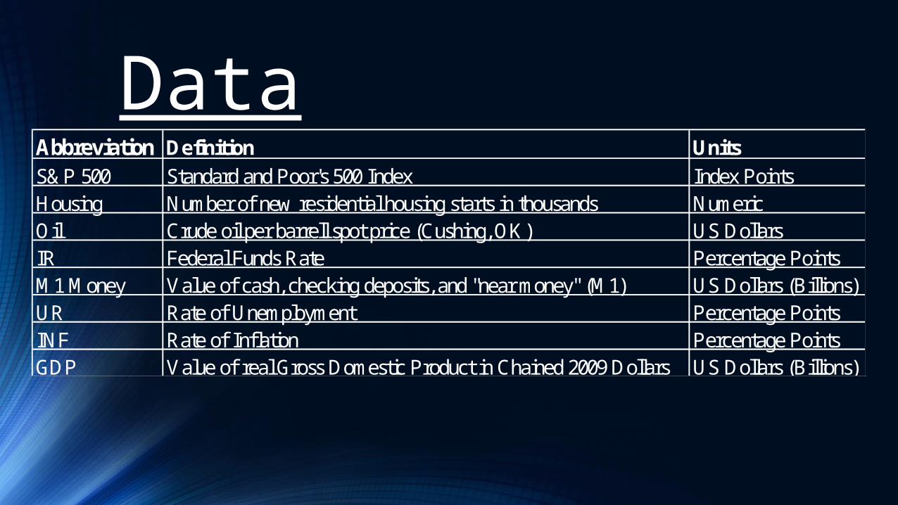
DataAbbreviation Definition UnitsS&P 500 Standard and Poor's 500 Index Index PointsHousing Number of new residential housing starts in thousands NumericOil Crude oil per barrell spot price (Cushing, OK) US DollarsIR Federal Funds Rate Percentage PointsM1 Money Value of cash, checking deposits, and "near money" (M1) US Dollars (Billions)UR Rate of Unemployment Percentage PointsINF Rate of Inflation Percentage PointsGDP Value of real Gross Domestic Product in Chained 2009 Dollars US Dollars (Billions)

Descriptive StatisticsDescriptive Statistics S&P 500 Housing Oil IR UR GDP INF M1 MoneyMean 1457.15 83.74 81.61 1.38 6.92 15159.30 1.75 2010.33Standard Error 55.67 5.83 3.26 0.32 0.30 95.65 0.16 92.81Median 1408.47 76.30 81.57 0.15 6.60 14963.36 1.80 1819.00Range 1270.02 148.50 96.31 5.19 5.60 2115.01 5.30 1701.30Standard Deviation 356.49 37.31 20.90 2.03 1.89 612.45 1.00 594.28Sample Variance 127082.15 1392.06 436.93 4.11 3.58 375094.69 1.00 353173.28Minimum 797.87 31.90 44.75 0.07 4.40 14355.56 -0.70 1367.80Maximum 2067.89 180.40 141.06 5.26 10.00 16470.57 4.60 3069.10

Initial Regression•S&P500 = -1500.23 - 0.05Housing - 0.267Oil + 165.53IR + 42.06UR + 0.06GDP - 14.79INF + 0.80M1 Money

•Statistically Significant Variables: Interest Rate and M1 Money.

•Statistically Insignificant Variables: Housing Starts, Oil Price, Unemployment Rate, GDP, and Inflation.

Initial Regression Output

Model Summaryb

Model R R Square

Adjusted R

Square

Std. Error of the

Estimate Durbin-Watson

1 .968a .937 .924 98.27502 1.028

Coefficientsa

Model

Unstandardized Coefficients

Standardized

Coefficients

t Sig. B Std. Error Beta

1 (Constant) -1500.230 1715.775 -.874 .388

Housing -.050 .912 -.005 -.055 .956

Oil -.267 .880 -.016 -.304 .763

IR 165.534 29.550 .941 5.602 .000

UR 42.058 23.108 .223 1.820 .078

GDP .058 .125 .100 .463 .646

INF -14.786 20.024 -.041 -.738 .465

M1_Money .801 .151 1.336 5.306 .000

Multi-Collinearity•The data exhibited symptoms of multi-collinearity as the R-squared was very high at 0.937 even though the initial regression only yielded two significant variables.

•Auxiliary Regressions Show: • Housing Starts highly correlated with Interest Rate (.754) and Unemployment (.815).

• Money Supply highly correlated with GDP (.930).

Autocorrelation•Durbin-Watson test indicates positive autocorrelation exists in data.

•Addition of a time trend variable was not statistically significant at a .05 level.

•First Differences regression yielded a lower Durbin-Watson statistic than the original regression.

F-Test•F-test to determine if statistically insignificant variables can be dropped from the equation.H0: B2=B3=B5=B6=B7=0HA: H0 is false

•Result: Do Not Reject Null Hypothesis.

New Model•S&P 500=f(IR, M1 Money)•S&P500=-258.169+119.775IR+0.771M1 Money

New Model OutputModel Summaryb

Model R R Square

Adjusted R

Square

Std. Error of the

Estimate Durbin-Watson

1 .964a .928 .925 97.83989 .926

Coefficientsa

Model

Unstandardized Coefficients

Standardized

Coefficients

t Sig. B Std. Error Beta

1 (Constant) -258.169 83.051 -3.109 .004

INT 119.775 10.391 .681 11.527 .000

M1_Money .771 .035 1.285 21.763 .000

Model ComparisonCoeffi cients P-Value Coeffi cients P-Value

Constant -1072.86 0.287 -258.17 0.004Housing Starts 0.02 0.984Oil Price -0.29 0.757Interest Rate 167.56 0.000 119.78 0.000Unemployment Rate 40.88 0.083GDP 0.03 0.71Inflation Rate -14.02 0.489M1 Money Supply 0.8 0.000 0.771 0.000

Model 1 Model 2Model Comparison

Results•The interest rate and the money supply have statistically significant effects upon the S&P 500 Index.

•For every one percentage point increase in the federal funds rate, the S&P 500 is predicted to increase by 119.78 index points ceteris paribus.

•For every one billion dollar increase in the M1 money supply, the S&P 500 is predicted to increase by 0.77 index points ceteris paribus.

Conclusion•This model can be used to predict future values of S&P 500 Index using readily available economic data. An R-squared of .928 indicates that this model should accurately predict these future values.

•Predicted future interest rates and money supply levels can be used to estimate a range of possible S&P 500 values given these predicted future economic conditions.

Conclusion•Model 2 estimates S&P 500 Index to be 2,122.5 on January 1, 2016.• Actual S&P 500 Index on January 1, 2016 was 2,049.8.

•Model 2 estimates S&P 500 Index to be 2,218.5 on April 1, 2016. • Actual S&P 500 Index on April 1, 2016 was 2,072.8.

•Model 2 estimates S&P 500 Index to be 2,212.8 on July 1, 2016.