Draft – Please do not cite August 2008 Development Economics: Theory, Empirical Research and Policy Analysis Julie Schaffner

Chapter 3 Economic Growth: Introduction

According to the umbrella definition offered in Chapter 1, the objective in development is “sustained improvement in the well-being of a country’s many people”. In Chapter 2 we examined possible definitions and measures of “well-being” at the level of a household. For this chapter and the next we shift from the micro level of the household to the macro or aggregate level of an entire country, and consider what is involved in defining and measuring overall development success. In this chapter we focus on a measure of aggregate change that has long been considered central to development success: economic growth, or growth in a country’s average income. While at first the concept of economic growth might sound far removed from the widespread and multidimensional improvements in well-being sought by development actors and described in Chapter 2, most analysts would agree that economic growth is of fundamental importance to long-term development success. In the absence of growth, average income remains constant, and any efforts to channel more income to the poor or to use income to provide more education or health care must channel income away from others. Where average income is just $517 per year, as in Sierra Leone, the best that can be done through such redistribution is to create widely shared poverty. Thus long-term development with the potential to erase vast differences in living standards across countries must involve increases in average income, or economic growth. This chapter first discusses how economic growth is defined and measured, and elaborates on its relationship to the larger concept of economic development. It then raises the natural question: What causes rapid economic growth? We begin answering this question by describing the kinds of change in the nature of economic activity that give rise to economic growth. We will refer to these changes as the “proximate” sources of economic growth. Later in the chapter we begin digging deeper, into the decisions and decision-makers through which these processes are set into motion, and the ways in which the policies of governments and other development actors, and the larger institutional frameworks within which these actors work, might influence these decisions. The rest of the textbook digs deeper still into the causes of good growth performance, building a rich model of how people, interacting with each other in market and non-market institutions, make decisions that shape rates of economic growth (as well as other development outcomes).

What is economic growth and how does it relate to the broader development objective?

Economic growth is defined as growth in an economy’s average income. In principle, average income is just the total value of income earned in any form, from any source, by

anyone in the country (as per the definition of income offered in Chapter 2), divided by the number of people in the country. Economic growth takes place, then, when the total income in the economy grows faster than the population. An economy’s total income equals the total value of its production, because people derive income only by engaging in the production of goods and services, and because all the value created through production activities must be “paid” out as income to someone in some form. Thus economic growth also requires that the total value of production grow faster than the population. Economic growth makes possible the shared, sustained improvements in well-being pursued by development actors. Increases in average income make it possible to increase income for some without necessarily having to reduce the income of others, and creates the potential for improvements that can be sustained for a long time. Increased income may flow directly into households, allowing them to purchase more goods and services through markets, or may be collected through taxation or charitable giving and used to expand the distribution of goods and services for which markets may not function well. Thus economic growth makes possible improvements in the many dimensions of current well-being that we discussed in Chapter 2. We will also see that economic growth arises when people take advantage of good investment opportunities. Thus, even before growth yields its tangible benefits, the conditions that give rise to growth may already be improving peoples’ dynamic well-being, as they enjoy improved opportunities to build better futures for themselves and their families. Unfortunately, success in economic growth does not guarantee complete success in development, for at least two reasons. First, average income can grow at a good pace even when the incomes of many individuals are stagnating or even declining. Thus while high rates of economic growth make possible widespread improvements in material living standards, they do not guarantee that the improvements will in fact be widespread. Second, as discussed in Chapter 2, increases in a household’s income do not guarantee that the household’s well-being is rising, because the improved income may be counter-balanced by reduced access to health care systems or greater fears regarding the future. Chapter 4 examines some of these potential differences between economic growth and development in more detail, and describes a variety of measures (related to reductions in the ills of poverty, inequality and vulnerability) that are complementary to growth rate measures for drawing inferences about development success at the aggregate level. Though economic growth is not identical to development, it is nonetheless crucial for long-run development success. It is thus important to understand the processes that underlie growth, and the ways in which intervention by governments or NGOs might affect the speed of growth.

How do we measure economic growth? The most common measures of economic growth are the average annual percentage growth rates in real per capita Gross Domestic Product (GDP) and real per capita Gross National Product (GNP). Gross Domestic Product (GDP) is defined as the total value

of final goods and services produced within a country’s borders during a specific period of time, such as a calendar year. The limitation to final goods and services excludes intermediate goods and services, which are used up in the production of other goods and services in the same period of time. For example, cotton thread is an intermediate good used up in the production of the final good, woven fabric. The value of intermediate goods and services produced within a country’s borders are not explicitly added in when calculating GDP, because their value is already included implicitly in the value of the final goods and services they were used to produce; including them again would lead to double counting. The difference between the value of intermediate goods and services used in a production activity and the value of the final output produced by the activity is called the activity’s value added. Calculating the total value of all final goods and services is equivalent to calculating the value added generated by every production activity in the economy, whether it produces intermediate or final goods and services.1 Final goods include both capital goods, which are used in the production of other goods and services, but are not used up during the period for which GDP is being measured, and consumption goods, which are used up during the period. In practice, obtaining accurate measures of GDP is difficult, especially in developing countries. Statisticians can only measure what they are able to observe. The typical approach to measuring the value of production is to observe goods and services as they pass through markets where transactions are recorded. Unfortunately, in some developing countries substantial fractions of agricultural production never pass through markets, because farm households consume their own produce. Growth and development often bring with them the spread of markets, as we will see in Chapter 6. As production that formerly took place outside of markets is drawn into markets, there may be some tendency for measured rates of growth in GDP to overstate true rates of growth in production. Where avoidance of tax laws and regulations is prevalent, many other goods and services also take place in black markets, outside the view of government statisticians. In some developing countries attempts are made to estimate these components of national product, but estimates tend to be based on weak data and on estimation methods that differ across countries. Yet other services and goods are produced by the governmental bureaucracy and offered without charge or for fees that do not represent their value. Accounting conventions for the calculation of GDP call for valuing the goods and services produced by government at their cost of production, which can be observed in government budget calculations, but may or may not provide an accurate representation of their true value.

1 Suppose a country contains only two industries, a final goods industry, which sells all of its output to consumers, and an intermediate goods industry, which sells all of its output to the final goods industry. The final goods industry produces its output using labor, capital and the intermediate good, while the intermediate good industry produces its output using only labor and capital. Let Y be the total value of final goods production and X be the total value of intermediate goods production. The value added produced in the final goods industry is equal to Y-X, while the value added in the intermediate goods industry is X. We can calculate the total value of GDP either by looking at the total value of production in only the final goods industry (Y) or by adding up the value added produced in both final and intermediate goods industries ((Y-X)+X=Y). Either way, we calculate that total GDP is equal to Y.

Gross National Product (GNP) is the value of final goods and services produced by domestic factors of production, whether at home or abroad. The distinction between GDP and GNP can be significant when countries’ labor or capital cross national borders to engage in production. The value of final goods and services produced by Brazilian labor and capital outside Brazil’s borders (by Brazilian workers who have migrated to other countries for work, or by Brazilian capital invested outside Brazil) is counted in Brazil’s GNP but not in its GDP. Similarly, the value of final goods and services produced by Japanese capital or labor within Brazil’s borders is counted in Brazil’s GDP but not in its GNP. Calculating GDP (or GNP) growth rates requires comparing the total value of goods and services produced in two different periods of time (e.g. the year 1990 and the year 2000). When the goods and services are valued using current prices (so that the goods produced in 1990 are valued using 1990 prices and the goods produced in 2000 are valued using 2000 prices), the resulting growth rate is a measure of nominal GDP growth. Nominal GDP might increase over time, either because the quantity and quality of goods and services increased, or because the prices of goods and services of given quality increased through inflation. Real GDP growth measures the portion of nominal GDP growth that can be attributed to increases in the quantity and quality of goods and services produced, rather than to price increases. The growth in real GDP from one year to the next is measured by using a single set of prices (often the prices in the first year) to value the quantities of good and services produced in both years. Measures of per capita growth seek to measure what is happening not to total income, but to the income available per person within the economy. Measures of per capita income are answers to the question: If we could redistribute all income until we achieve equality of incomes across people, without incurring any costs or losing any of the income in the process, what level of income would be enjoyed by everyone? Increases in per capita income indicate expansion of the level of material prosperity that everyone could share if income were distributed evenly.

Growth figures are usually reported as annual growth rates. This means that even when the period of interest is greater or less than one year, the average growth rate for that period is expressed as the growth that would occur over one full year at the observed pace. Growth rates are often expressed as annually compounded average rates. This means that the averages are calculated in a way that treats growth as a multiplicative process, in which growth during any one year leads GDP per capita to start the next year at a higher level of the base to which subsequent growth rates should be applied. For example, consider the table to the right describing the evolution of GDP in an economy that starts with GDP of 100 and grows at a steady annually compounded rate of 3 percent for 10 years. We can see compounding in the calculation of Year 2 GDP, which shows that the growth experienced from Year 1 to Year 2 (embodied in the final 1.03 factor) was applied not just to the original 100, but to 100*1.03, which was the new level of GDP attained in Year 1, as a

Year GDP Year 0 100 Year 1 100*1.03=103 Year 2 100*1.03*1.03=106.09

… Year 10 100*(1.03)10≈134.39

result of growth in the first year. The average annually compounded growth rate over a ten year period for a country that had GDP of G0 in Year 0 and G10 in Year 10 is the growth rate r (expressed, e.g. as r=.03 for a three percent growth rate) that solves the equation G0*(1+r)10=G10.

Empirical Growth Facts

Now that we know how measures of economic growth are constructed, we turn to a common source of data on economic growth, the Penn World Tables version 6.2 (Heston, et al., 2006), and review some basic facts regarding historical experience with economic growth around the world. What rates of economic growth are “fast” and “slow”? Figure 3.1 describes the range of average annually compounded growth rates over the period 1960-2000. The highest average growth rate achieved among the 98 countries for which adequate information was available was Taiwan’s 6.68 percent, while the lowest was Madagascar’s -1.07 percent. (The negative sign in this growth rate means that on average over this period income per capita was shrinking at more than 1 percent per year.) The most common growth rates were in the 2.5 to 3.0 percent range.

Figure 3.1 Average Annual Growth Rates in GDP per capita, 1960-2000

0 5 10 15 20 25 30 35 40

>6.5%

6.0% ~ 6.5%

5.5% ~ 6.0%

5.0% ~ 5.5%

4.5% ~ 5.0%

4.0% ~ 4.5%

3.5% ~ 4.0%

3.0% ~ 3.5%

2.5% ~ 3.0%

2.0% ~ 2.5%

1.5% ~ 2.0%

1.0% ~ 1.5%

0.5% ~ 1.0%

0% ~ 0.5%

-0.5% ~ 0%

-1.0% ~ -0.5%

-1.5% ~ -1.0%

Ave

rag

e an

nu

al g

row

th r

ate

Number of countries

Example

Taiwan

Korea, Republic of

China

Hong Kong

Singapore, Malaysia, Thailand

Japan

Portugal, Sri Lanka, Mauritius, Romania

Indonesia, Norway, Ghana, Greece

Austria, Lesotho, Panama, Italy, Pakistan

United States, Turkey, Denmark, Syria

Mexico, Colombia, Switzerland, Philippines

Ethiopia, Ecuador, South Africa, Nepal

Argentina, Zimbabwe, Peru

Uganda, Bolivia, Venezuela, Kenya

Rwanda, Nigeria, Zambia, Jordan, Senegal

Nicaragua, Chad, Niger

Madagascar

Source: Calculations employing Heston, et al. (2006). The Rule of 72. One way of understanding how large or small annually compounded growth rates are is to employ the “rule of 72”. This useful mathematical approximation tells us that to estimate roughly how many years it will take to double income per capita when the annually compounded growth rate is g percent, we can simply divide g into the number 72. For example, at a growth rate of 3 percent, you can expect to double income per capita in roughly 72/3=24 years. At a growth rate of 5 percent, you could expect to double income per capita in less than 14 and a half years. With growth rates near 7 percent, the top performers in Table 3.1 doubled their average incomes nearly four times in four decades! Growing at 2.48 percent, the United States doubled its average income only once; other countries failed even to increase their average income.

Lack of growth in many poor countries. If countries with low per capita income are ever to catch up to the levels of per capita income enjoyed in the world’s richer countries, then they must experience higher rates of economic growth. Figure 3.2 allows us to ask whether poorer countries have tended to grow more rapidly than richer countries over the last 40 years, and thus whether poorer countries have shown any tendency for their per capita incomes to “catch up” with per capita incomes in the richer countries. The horizontal axis measures GDP per capita in 1960, while the vertical axis measures the rate of economic growth. The scatter plot shows no strong tendency for poor countries to grow more rapidly than rich countries. Indeed, the simple average of the growth rates appears even to rise slightly as the initial level of GDP per capita rises, as indicated by the regression line drawn through the middle of the scatter plot. The figure also demonstrates, however, that there is great diversity in growth rates at most income levels, and especially at lower income levels. Some poorer countries grew very fast over this period, partially closing the gap in per capita incomes between them and the richer countries, while other poor countries stagnated, the per capita income gap between them and the richer countries growing wider over the period.

Figure 3.2 No Systematic Tendency for Poorer Countries to “Catch Up”

-2.0

-1.0

0.0

1.0

2.0

3.0

4.0

5.0

6.0

7.0

0 2000 4000 6000 8000 10000 12000 14000 16000

GDP per capita ,1960

Gro

wth

rat

e 19

60-2

000(

%)

Source: Heston, et al. (2006).

Historical studies of average income around the world suggest that if we were to look at growth rates over a longer period, reaching further back into history, we would see an even stronger tendency for per capita incomes in richer countries to pull ahead of those in poorer countries. These studies argue that average incomes were much more similar across countries in 1870, a date associated with the beginnings of modern economic growth, than they are today (Pritchett, 1997). The vast current differences in per capita

income that we observed in Chapter 1, with GDP per capita over 100 times greater in the richest countries compared to the poorest countries – must be the result of “divergence, big time”, as rapid economic growth in today’s rich countries allowed them to pull away from the rest. Regional differences in the level and variability of growth rates. The level and variability of economic growth rates have tended to vary across geographic regions of the world. Table 3.1 divides the 84 countries for which adequate data are available, and that had populations of at least 1 million in 1960, into geographic regions of the world. Within each region it gives equal weight to each country (regardless of the country’s population size) when calculating medians across countries for various growth statistics. The first two columns report median average growth rates in the periods 1960-1980 and 1980-2000. The third column reports the median across countries within a region of a measure of a country’s volatility in growth rates over time: the standard deviation of its annual growth rates over 1980-2000. While growth rates in East Asia and the Pacific have tended to exceed growth rates in the OECD in both periods, and growth rates in South Asia have exceeded growth rates in the OECD in the more recent period, growth rates have tended to be lower in many other parts of the developing world, especially in Sub-Saharan Africa. Growth has also tended to be more volatile throughout the developing world relative to the industrialized countries. Again, Sub-Saharan Africa stands out as experiencing much more volatile growth than other regions. The table also demonstrates some tendency for growth rates around the world to slow after 1980. More detailed data would demonstrate the existence of a few notable exceptions, such as China and India, in which growth took off after 1980. Additional data would also reveal a much more recent acceleration of growth in Sub-Saharan Africa (Arbache and Page, 2008).

Table 3.1 Growth Experience by Region

Region Within-Region Median

of Average Annual Growth Rates

1960-1980

Within-Region Median of Average

Annual Growth Rates 1980-2000

Within-Region Median of Standard Deviation of

Annual Growth Rates 1980-2000

OECD All Low and Middle Income Countries

3.63

2.18

1.93

0.72

2.09

4.29

Eastern Europe and Central Asia East Asia and the Pacific Middle East and North Africa Latin America and the Caribbean

5.04

5.00

3.27

2.21

0.98

4.21

0.76

0.30

4.82

4.21

4.17

3.88

South Asia Sub-Saharan Africa

2.79

0.91

2.97

0.28

2.68

5.75 Source: Heston, et al. (2006).

Proximate Sources of Economic Growth Real per capita income increases when the total value of goods and services produced by the economy rises faster than the population. If we think of goods and services as the “outputs” of the economy’s production activities, and recognize that people provide a key “input” (labor), this suggests that economic growth takes place when the economy’s workers become more productive on average. Identifying the proximate sources of economic growth, or the changes in economic activity that give rise to growth, thus requires identifying types of economic change that increase aggregate labor productivity, which is the average value of output produced per worker in the economy’s farms, family enterprises, firms and other production operations. The contemporary view of the proximate sources of growth exposited in this section is much broader than the view that shaped economic thought about growth a half century ago, in the early days of international interest in economic development. Chapter 4 describes how interaction between theoretical and empirical research over the intervening decades helped propel economists toward the broader view that shapes economic thought today. Analytical framework: Firms, production functions and labor productivity Basic production concepts. When looking for sources of labor productivity increase, it is useful to develop a working mental model of the people and processes involved in the production of goods and services. This section briefly reviews the basic concepts that economists employ for organizing their thinking about production and productivity. Production takes place when people we call producers or entrepreneurs decide to bring together workers, equipment and other factors of production to create goods and services. Entrepreneurs may have Harvard MBAs and start multi-million dollar corporations, or may be illiterate household heads operating small farms or selling cold drinks from a road-side stand. We will follow common practice in referring to the production operations started by these entrepreneurs as firms, but must recall that many “firms” in developing countries are much smaller, more informal and more embedded within households than are firms in developed countries. The most obvious and important classes of factors of production are labor and capital, where the term “capital” (or “physical capital”) refers to machines, tools, buildings and other equipment and structures whose services are employed by workers in the production process, and that are long-lasting (in the sense that they are not used up in a single year’s production activities). Sometimes labor and capital are the only inputs used in a firm’s production (as might be the case when a family business sells carpentry services); but often firms combine labor and capital with raw materials (such as raw

cotton), intermediate goods (such as cotton thread) or services (such as electricity) to produce higher value goods (such as woven cloth). Either way, we can think of firms as using the basic factors of production (labor and capital) to produce value added (the properties of the woven cloth that make it more valuable than the raw materials and intermediate inputs that went into its production). The labels “labor” and “capital” are, of course, short-hand labels for long lists of diverse inputs to production. Workers of diverse levels of education, training and age, and who differ in innate skills and interests, tend to engage in production processes in different ways and to different effect. Similarly, physical capital includes simple hammers and crow-bars, on the one hand, and sophisticated computer-controlled manufacturing equipment on the other. Economists pay special attention to differences among workers’ skills and abilities that arise out of purposeful investments in education, training and health. Like investments in physical capital, these investments create assets with the ability to increase workers’ productivity and income for many years into the future. Economists have thus given the name “human capital” to the skills and abilities that workers might bring into production as a result of past education, training, nutrition and health care. Entrepreneurs’ ability to turn labor, physical capital and human capital into output is limited by the technology, or the array of technological options at their disposal. For any quantities of labor and capital of various types that producers employ, the available technology determines the maximum quantity of output that the firm can achieve. Though the technology constrains producers, it does not necessarily limit them to a single way of producing an item. It may be possible, for example, to produce a given quantity of output with varying combinations of labor and capital. The technological possibilities a firm faces may change over time, whether through informal learning, purposeful invention or technology purchase, allowing the firm to obtain more output (or higher value output) from given quantities of the inputs. The forces of such technical change increase productivity, and may also modify the relative importance in production of various types of labor and capital inputs. Production functions. Economists organize their thinking about technological possibilities and productivity around the concept of a production function, which is a mathematical representation of the maximum output the firm can achieve from any combination of inputs it might choose to employ. In general, the production function describes how the maximum quantity of output achievable by a firm is related to a detailed list of inputs, including quantities of labor supplied by workers with different types and amounts of human capital, quantities of capital equipment of differing vintages, and more. Here we will keep things simple, and prepare ourselves for thought about the average productivity of workers, by assuming that what matters for determining output within a given technology is just the total number of workers (L), and the total value of capital (both physical capital and human capital) with which those workers are combined (K). Under these assumptions, we can write the production function this way:

(1) Y = F(L, K ; A) where Y is the maximum quantity of output that can be produced in a given period of time, given particular values of L and K, and F(.) is a function that describes the relationship between input levels and maximum output.2 We allow for the possibility of technical change by including as an argument of the function the parameter A, which is an index of the current level of technology. We separate A from L and K by a semi-colon, to emphasize the distinct roles of inputs (L and K), on the one hand, and the technology index (A), on the other. We expect this production function to satisfy certain sensible properties. First, we expect that the function F(.) is increasing in both inputs, meaning that if the quantity of either or both of the inputs (labor or capital) increases, output increases. Second, we expect the production function to exhibit diminishing marginal product of either input. The marginal product of labor (capital) is the increase in output associated with a one unit increase in labor (capital), while holding the quantity of capital (labor) constant.3 By assuming that the production function is increasing in its inputs, we have already assumed that these marginal products are positive. When we say that we expect these marginal products to be diminishing, we are expressing the sensible expectation that each successive increase in the quantity of an input (while holding the quantity of the other input constant) will increase output by less. For example, if we hold the number (and human capital attributes) of workers in a textile factory constant, we may nearly double output if we increase the number of looms per worker from one to two. Rather than remaining idle after setting up the sole loom and setting it into motion, the worker may now use that time to set up the second loom. Eventually, however, as the number of looms increases, it will become harder and harder for the worker to keep every loom working at full capacity. Output may continue to increase as the worker is given additional looms to work with, but the increments to output will become smaller and smaller. Third, we expect that the function F(.) is increasing in the parameter A, indicating that if technological knowledge improves (which we denote by an increase in A), the maximum quantity of output derived from given levels of labor and capital increases. A potentially important difference in the nature of production functions for products of different types has to do with the “returns to scale” exhibited by the function. We can evaluate whether a production function (at a given level of technology) has constant, increasing or decreasing returns to scale by asking what happens to output when we double the amount of both inputs (K and L). If output just doubles, then the technology exhibits “constant returns to scale”. If output more than doubles, the technology exhibits

2 Following standard practice, we include only basic factors of production as arguments of the production function, and do not also include raw materials or intermediate inputs as arguments. This makes sense if we think of Y as the maximum value added that may be created by L and K within the current technology. That is, Y is the quantity of improvements to raw materials and intermediate inputs that are effected by L and K. 3 Mathematically, the marginal product of labor (capital) is equal to the partial derivative of the production function with respect to labor (capital). The partial derivative function describes how the size of the marginal product depends on the values of the arguments (capital and labor).

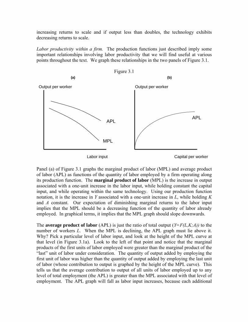
increasing returns to scale and if output less than doubles, the technology exhibits decreasing returns to scale. Labor productivity within a firm. The production functions just described imply some important relationships involving labor productivity that we will find useful at various points throughout the text. We graph these relationships in the two panels of Figure 3.1.

Figure 3.1 (a) (b)

Labor input Capital per worker

Output per worker Output per worker

MPL

APLAPL

Panel (a) of Figure 3.1 graphs the marginal product of labor (MPL) and average product of labor (APL) as functions of the quantity of labor employed by a firm operating along its production function. The marginal product of labor (MPL) is the increase in output associated with a one-unit increase in the labor input, while holding constant the capital input, and while operating within the same technology. Using our production function notation, it is the increase in Y associated with a one-unit increase in L, while holding K and A constant. Our expectation of diminishing marginal returns to the labor input implies that the MPL should be a decreasing function of the quantity of labor already employed. In graphical terms, it implies that the MPL graph should slope downwards. The average product of labor (APL) is just the ratio of total output (Y=F(L,K;A)) to the number of workers L. When the MPL is declining, the APL graph must lie above it. Why? Pick a particular level of labor input, and look at the height of the MPL curve at that level (in Figure 3.1a). Look to the left of that point and notice that the marginal products of the first units of labor employed were greater than the marginal product of the “last” unit of labor under consideration. The quantity of output added by employing the first unit of labor was higher than the quantity of output added by employing the last unit of labor (whose contribution to output is graphed by the height of the MPL curve). This tells us that the average contribution to output of all units of labor employed up to any level of total employment (the APL) is greater than the MPL associated with that level of employment. The APL graph will fall as labor input increases, because each additional

unit of labor draws the average down, but the slope is shallower than the slope of the MPL curve. Panel (b) of Figure 3.1 graphs the average product of labor (APL) as a function of the quantity of capital employed by a firm operating along its production function. In this graph, rather than varying the labor input while holding capital and technology constant, we are varying the capital input while holding the quantity of labor and technology constant. Because we are holding the quantity of labor constant, an increase in the capital input is also an increase in the quantity of capital per worker. We label the horizontal axis “capital per worker” rather than “capital”, because thinking about capital in “per worker” terms will be useful as we think about determinants of growth in labor productivity. Diminishing returns implies that the slope of this graph is positive but declining as we move to the right. Holding the quantity of labor constant, initial increases in the quantity of the physical or human capital with which it is combined increase the productivity of labor quite a bit. Eventually, however, additional increments of capital generate smaller and smaller increments in output per worker, as the unchanging number of workers finds it harder and harder to make full use of the skills and equipment at their disposal. We could introduce changes in the level of technology (A) into either graph in Figure 3.1. Figure 3.2 illustrates the implications of technical change for a graph like 3.1(b). By definition, if we increase A while holding both L and K constant, output increases. An increase in A must then cause the APL curve to shift up, as illustrated by the shift from curve APL1 to curve APL2. Throughout the graph we are holding the quantity of labor constant, and at any point along the horizontal axis we are holding the quantity of capital constant, so an increase in A must associate any quantity of capital per worker with a higher value of maximum output.

Figure 3.2

Capital per worker

Output per workerAPL2

c

ab

d

Figure 3.2 offers a useful way of organizing thought about potential sources of productivity increase that might be experienced within individual production enterprises. Consider first a firm facing the technological options associated with curve APL1 and operating at point a. This firm is “on its production function”, implying that it is managing to get the maximum possible output out of the labor and capital inputs it employs, given the technological options available to it. Three sorts of change might increase labor productivity in this firm. It could move to the right along the APL1 curve, to a point like b, either by (a) increasing physical capital per worker or (b) by increasing human capital per worker. It could instead shift up to point c through (c) the acquisition of new technology that allows it to get more output from the same quantities of labor, physical capital and human capital. (It might, of course, also engage in more than one of these changes simultaneously.) A fourth possible source of increase in labor productivity within a firm is possible for a firm facing the technology associated with curve APL1 and operating at point d. Such a firm is technically inefficient, meaning that it is failing to get as much output as is technologically possible given the input quantities it employs. (We explore possible reasons for this below.) Such a firm could increase labor productivity by increasing its technical efficiency, moving from point d up toward point a. Labor productivity averaged across all firms and workers. What matters for economic growth is not just productivity in a single firm, but aggregate labor productivity, which is the total value of all goods and services produced in the economy (GDP) divided by the total number of workers in the economy. Clearly aggregate labor productivity has something to do with the levels of labor productivity achieved in the economy’s many firms, and is thus related to the notions of MPL and APL defined above. To figure out the precise relationships between these concepts, we must begin by recognizing that while the MPL and APL measures were expressed in units of physical output per worker, which cannot be meaningfully compared and averaged across firms producing different kinds of output, aggregate labor productivity is expressed in dollars or pesos (of valuable output created) per worker. We can translate MPL and APL measures into dollar terms, rendering them useful for examining matters of aggregate labor productivity, by multiplying them by the output prices relevant to each firm (p), and calling the resulting measures the value of the marginal product of labor (VMPL=p*MPL) and the value of the average product of labor (VAPL=p*APL). Having translated our firm-level productivity measures into comparable dollar terms, we can now imagine calculating aggregate labor productivity by: (1) looking at how all labor in the country is allocated across diverse firms and other “uses” (including unemployment), (2) observing the VAPL in each firm or use, and (3) calculating the weighted average of all these VAPLs, where greater weights are given to the VAPLs associated with activities in which larger fractions of the country’s labor are employed.4

4 Aggregate labor productivity is the ratio of GDP to the total number of workers, L. GDP equals the sum p1Y1 + …. + pnYn, where Y1,…,Yn are the quantities of goods and services produced across all possible firms or uses of labor, and p1,…,pn are the respective prices per units of output. L is the sum of the

This has important implications for thinking about sources of growth in aggregate productivity. First, all four potential firm-level sources of productivity growth illustrated in Figure 3.2 remain relevant for thinking about productivity growth at the aggregate level. Increases in economy-wide stocks of physical or human capital, relative to the stock of labor, will tend to imply increases in the ratios of physical and human capital to labor within at least some firms, implying aggregate productivity increase. Similarly, technological change and increases in efficiency within firms will contribute to aggregate increases in the overall value of goods and services derived from the same inputs. The larger are the sets of firms in which technological change and efficiency improvements take place (in the sense of employing larger fractions of the labor force), the greater will be the impact on aggregate average labor productivity and the rate of economic growth. Second, aggregate productivity can also arise through the re-allocation of labor across activities within the economy. Most obviously, if one of the current “uses” of labor is unemployment, then changes in economic performance that shift some labor out of unemployment (where labor productivity may be zero) into productive firms (where labor productivity is greater than zero) will increase overall average labor productivity. Similarly, if some labor is employed in what we will call (below) “rent-seeking” activities, which use up productive resources but do not produce additional output, then structural changes that shift labor away from those activities into productive firms will again increase aggregate labor productivity. Under certain circumstances, aggregate labor productivity may also be increased by shifting labor (or capital) across productive sectors of the economy (e.g. shifting labor from agriculture to manufacturing), or across firms within a productive sector. One example arises if the value of the marginal product of labor (VMPL) is not equal across sectors or firms. If this is the case, then shifting workers away from firms in which the VMPL is lower to firms in which the VMPL is higher will increase aggregate labor productivity. To see this recall that the marginal product of labor is defined as the number of units by which total output would increase (decrease) if one worker were added (taken away), while holding all other inputs and technology constant. The value of the marginal product of labor is just this quantity multiplied by the dollar value of a unit of output. If the VMPL is higher in firm A than in firm B, then if you take one worker away from Firm B, the value of output lost there is less than the value of output gained when the one worker is added to Firm A. Hence the total value of output in the economy rises as a result of this shift in labor use across firms. An important result in intermediate microeconomic theory is that if all markets in an economy work perfectly, then the VMPL of identical labor should be equalized across uses throughout the economy. In such a case, there would be no scope for increasing

quantities of labor allocated to each of the possible uses: L1+…+Ln. With a little algebra it is easy to show that aggregate labor productivity GDP/L may be re-expressed as (L1/L)VAPL1 + … + ((Ln/L)VAPLn, where (L1/L) is the share of total labor devoted to firm or use 1, and VAPL1=p1Y1/L1 is the value of the average product of labor in firm or use 1.

productivity simply by shifting labor across uses. In the more complicated real world, however, both market failures and policies may have the potential to prevent equalization of the VMPL across all sectors and firms, opening up the potential for aggregate productivity growth through such shifts of labor across sectors and firms, a possibility we return to at several points throughout the text. Another example of the potential for shifts in input allocation across firms to increase aggregate labor productivity arises when production technologies are subject to increase returns to scale (as defined above). If production of a good is characterized by increasing returns to scale, and its production currently takes place in many small firms, then, even though the marginal product of labor may be equated across those firms, it would be possible to increase aggregate labor productivity by pooling the inputs from the many small firms into a single larger firm. In Chapter 6 we will examine the forces that might keep production establishments small in early stages of development, but may change in ways that allow increases in scale, contributing to growth in average labor productivity. The analytical framework developed in this section raises the possibility of aggregate productivity growth arising through many channels. The next 3 sub-sections expand upon the potential importance of these channels as sources of economic growth in developing countries, grouping them into the categories of factor accumulation (increasing physical capital per worker or human capital per worker), total factor productivity increase (technological change, within-firm productivity increases, productivity enhancing re-allocations across sectors and firms), and reductions in waste (reductions in unemployment and reductions in rent-seeking activities). Sources of productivity growth: Factor Accumulation Increases in physical capital per worker. Imagine a small textile manufacturing firm, in which workers come together with machines (looms) and intermediate inputs (cotton thread) to produce a higher value output (woven textiles). Labor productivity is given by the total value added produced by the firm (i.e. the value of textiles produced less the value of thread used up in producing the textiles) divided by the number of workers. Perhaps the most obvious way to increase labor productivity in such a firm is to provide workers with more, larger or better looms. (This would correspond to a movement from point a to point b in Figure 3.2.) Similarly, an obvious way to increase labor productivity in the economy as a whole is to increase the average value of physical capital per worker, making workers more productive by giving them more and better equipment to work with. Cross country data suggest that there is plenty of room for developing countries to increase productivity by increasing capital per worker. Standard measures of the value of the physical capital stock, expressed on a per-worker basis, are on the order of $700 per

worker in Tanzania, $1900 in Ghana, $6000 in India, $13,000 in the Philippines, $31,000 in Brazil, and $146,000 in the United States.5 Increases in human capital per worker. Return to the imaginary textile factory. Several characteristics of the workers themselves may be improved in ways that increase the value of textiles they produce using the same machines and equipment. Workers with greater reading and calculating skills may be better able to adjust machine speed and tension in response to changing conditions in raw material properties, allowing them to reduce the frequency of machine failure and down time. Workers with superior training might be able to reduce the rate of flaws, increasing the value of the resulting fabric. Workers who are better nourished and healthier will work more rapidly, with fewer breaks and fewer sick days. (Increases in human capital per worker provide another explanation for a movement from point a to point b in Figure 3.2.) Again, cross country data suggest that there is plenty of room for increase in human capital per worker in the developing countries. According to Barro and Lee’s (2001) calculations, in rich countries 71.2 percent of the population had at least some secondary education, while 28.1 percent had at least some post-secondary education. By contrast, in developing countries taken altogether, only 31.1 percent had at least some secondary education, while only 6.5 percent had at least some post-secondary education, and 34.4 percent had no schooling at all! Education stocks are even lower in Africa, where only 2.2 percent of the population has any post-secondary education, 19.2 percent have at least some secondary education, and 42.8 percent have no schooling. On top of this, as we will see in Chapter 15, in countries where children get fewer years of schooling, the quality of schooling tends to be lower as well. Human capital differences across countries are further compounded by the greater tendency for workers in developing countries to be malnourished and unhealthy. One of the most telling ways to describe cross-country difference in health is with statistics on average life expectancy, which in 2005 was 79.4 years in high-income OECD countries, but only 54.5 years in the least developed countries, a difference of 25 years (UNDP 2008)! Sources of productivity growth: Increases in Total Factor Productivity Economists have paid increasing attention over the last five decades to reasons why workers’ productivity might rise even when the average amounts of physical and human capital with which they work are held constant. We say that firms’ total factor productivity (or TFP) rises when the value of output derived from given quantities of labor, physical capital and human capital rises. For an introduction to the measurement of TFP, see Box 3.1. The growth accounting and development accounting exercises within which TFP is measured tend to indicate that growth in TFP has played an important role in explaining historical growth around the world, and that differences

5 These numbers are estimated using the perpetual inventory method described in Caselli (2005), employing the Penn World Tables data (Heston, et al., 2006). They are reported in 1996 dollars per economically active member of the population.

across countries in TFP are also crucial for understanding current labor productivity differences across countries.

Box 3.1 Growth Accounting, Development Accounting and Total Factor Productivity

Researchers have long been interested in the question: Which of proximate sources of productivity increase seem to have been the most important empirically, whether for explaining increases in labor productivity over time within a single country, or for explaining differences in levels of labor productivity across countries today? This research has taken special interest in quantifying the relative contributions of two broad categories of proximate growth sources: factor accumulation (including increases in physical and human capital per worker) and growth in “total factor productivity” (a catch-all term including all the other sources of productivity growth described in the text). Such studies are motivated by the hope that identifying the most important sources of historical growth or productivity differences will provide guidance to researchers as they seek to dig deeper into the identification of policies with greatest potential to speed future growth. Growth accounting exercises, which originated in the 1960s, seek to identify the shares of historical growth (in one or more countries) that can be attributed to factor accumulation and TFP growth. They are based on highly simplified and restrictive assumptions regarding the process through which a country’s GDP is produced. Rather than acknowledging the existence of many firms and other possible uses of a country’s capital and labor, the method essentially treats the entire economy as if it were a single firm, and models total GDP (Y) as a simple function of the total quantities of physical capital (K), labor (L), and human capital per worker (h). (Many earlier studies ignored human capital as an input to aggregate production.) Furthermore, this production function is assumed to take a very simple form. For example, a study might posit that (1) Y = AKα(Lh)1-α where Lh can be interpreted as “effective” or “quality-adjusted” labor, α is a technological parameter defining the exact way in which Y responds to changes in K and Lh, and A is an index of Total Factor Productivity (TFP). As long as α takes a value between zero and one, this production function exhibits diminishing marginal returns to both K and Lh, a property we would expect most production functions to satisfy. It also exhibits “constant returns to scale”. Dividing through by L to turn this into a statement about GDP per capita (lower case y), we get (2) y = Akαh1-α where k=K/L is physical capital per worker. The relationship relates GDP per capita in a specific way to the levels of capital per worker and human capital per worker in the

economy. Starting with (2), it is easy to show (see problem 3 at the end of the chapter) that (3) gy = gA + αgk + (1-α)gh where gy, gA, gk and gh are the percentage growth rates in GDP per capita, TFP, physical capital per worker and human capital per worker. Equation (3) relates the GDP growth rate in a very specific way to rates of factor accumulation and TFP growth. Growth accounting exercises involve choosing a value for α that is thought to give a good representation of technological realities, measuring gy, gk and gh, plugging all these numbers into equation (3), and then “backing out” a value for gA, which is the only remaining unknown in the equation. If researchers measure gy=4 (percent per annum), gk=3 and gh=2, and estimate α=.3, then they would conclude that of the overall 4 percentage points of growth in GDP per capita, .3*4=1.2 percentage points are attributable to growth in physical capital per worker, .7*2=1.4 percentage points are attributable to growth in human capital per worker, while the remaining 4-1.2-1.4=1.4 percentage points represent growth in TFP. One critical challenge in carrying out a growth accounting exercise is to come up with an estimate of α. Two broad approaches have been taken to estimating this parameter. The first one is based on the observation that if the production function is well described by (1), then the marginal product of capital (MPK ) is equal to (αY)/K (the partial derivative of (1) with respect to K). Re-arranging this expression, we find that alpha equals (MPKK)/Y. If we are willing to assume that rental markets for capital are perfectly competitive, then MPK should equal the “rental rate” earned per unit of capital (r), for reasons reviewed in chapter 7. Substituting in r for the MPK, we find that α equals (rK)/Y, which is the ratio of total capital income in the economy to total GDP. It thus becomes possible to estimate α simply by observing the share of capital income in total income, a number that is close to .3 in the U.S. Another approach to estimating α employs econometric estimation. Relation (3) implies that the rate of economic growth (gy) should be equal to a linear function of gk and gh, in which the intercept is the rate of TFP growth and the coefficients on gk and gh are estimates of α and 1-α. This suggests that the rate of TFP growth and the coefficients α and 1-α can be estimated simultaneously by running regressions of per capita GDP growth on rates of growth in physical and human capital, employing observations from multiple years of growth experience. Another challenge in carrying out a growth accounting exercise is in constructing good measures of the rates of growth in physical and human capital per worker (as well as in GDP per capita). For examples of how such measures might be constructed, see Caselli (2005). Early applications of growth accounting methods focused on the developed countries, where studies tended to find an even split between the portions of growth attributable to factor accumulation and the portions attributable to TFP growth. Subsequent studies

have examined growth in a wider variety of countries. While in a few countries in Latin America and East Asia factor accumulation has appeared to play a significantly larger role (relative to TFP growth), many studies continue to find a nearly even split between factor accumulation and TFP growth for explaining historical growth (see Easterly and Levine, 2001). “Development accounting” exercises are very similar to growth accounting exercises, but examine differences in GDP per capita across countries rather than over time within individual countries. Rather than looking at growth rates over time in y, k and h, the studies look at percentage differences in y, k and h between any country of interest and a base country (often the U.S.). Such studies ask: how much of the overall variation in GDP per capita across countries at one point in time is attributable to differences in physical or human capital per worker and to differences in TFP. These studies, too, tend to find that differences in physical and human capital per worker explain about half the cross-country differences, while differences in TFP explain the other half (Caselli, 2005). Growth and development accounting exercises are useful for providing broad descriptions of the proximate sources of growth, and their results point to the importance of studying the processes of both factor accumulation and total factor productivity growth in efforts to understand the determinants of overall growth. But we must also recognize several profound limitations of such studies. First, while the results of these studies motivate interest in TFP growth as a source of economic growth in developing countries, they offer no insight into the relative importance of the highly diverse ways in which TFP might grow (as described in the text). Second, they are based on highly simplified assumptions regarding the nature of production relations in the economy. Indeed, efforts to relax some of the restrictive assumptions typically employed reveals that some of the standard results become quite fragile (Caselli,2005). Third, because TFP measures are “backed out” as the part of growth unexplained by factor accumulation, any errors in the measurement of factor accumulation or in the parameter α will introduce errors into the measurement of TFP, and all of this measurement is fraught with difficulty. Fourth, even if the assumptions on which these methods are based were valid, and the measures employed were accurate, the results at best describe past growth or present income differences, and need not be good predictors of what will be the most promising sources of future growth. Finally, even if they accurately revealed the most promising sources of future growth, they provide no insights into what sorts of policies might be required to achieve those promises. It might even be the case, for example, that policies promoting technological change will be required to stimulate physical capital accumulation, or that policies promoting human capital accumulation will be required to stimulate TFP growth.

Researchers such as Easterly and Levine (2001) provide additional reasons to suspect that TFP differences are important for explaining why productivity and income are so much lower in developing countries than in developed countries. First, if there were no difference in TFP across countries, then all countries would share the same level of technology (i.e. the same level of A in our production function notation) and all countries would be equally technically efficient. In the terms of Figure 3.2, all countries would be

on the same APL curve. If such were the case, then the only reasons for difference in labor productivity and per capita income would be differences in the quantities of physical and human capital per worker, which must be much smaller in the developing countries. The notion of diminishing marginal returns to capital would then imply that the marginal product of capital should be higher in the developing countries, and that the returns to investments in such capital should be relatively high there, causing physical and human capital to flow from the rich countries, where such capital is abundant and returns to investment are lower, to poor countries, where such capital is scarce and returns to investment are higher. But we do not observe such flows. Indeed, skilled laborers and capital tend to flow from poor countries, where they are scarce, to rich countries, where they are abundant! This suggests that the marginal return to capital is not uniformly higher in poorer countries. Within our production function framework, the most natural way to explain this is to suggest that lower levels of capital per worker (which would tend to increase the marginal product, given diminishing returns) are more than compensated by lower levels of technology and efficiency (which may reduce marginal products and the level of productivity). A second observation put forward by Easterly and Levine (2001) is that while rates of economic growth are highly volatile in developing countries (as seen above), rates of factor accumulation tend to remain much more steady from year to year, suggesting a role for the “something else” of total factor productivity in explaining growth rate fluctuations. For many years TFP differences were interpreted as primarily reflecting differences in the state of technological knowledge, but researchers increasingly hold open the possibility that TFP differences reflect differences in the technical efficiency with which technology is employed and productive resources are allocated across uses. 6 The following paragraphs describe quite diverse potential sources of TFP growth. Technical change. Think again about textile factories. Before the invention of water-, steam- and electric-powered looms, threads had to be woven across the emerging fabric by human effort. The invention of ways to let running water or steam provide the energy for such movement freed the weaving process from limitations in the speed and strength of human actions. With power looms, textiles may be woven at rates of six rows per second and faster, greatly increasing the quantity of textiles produced from a given number of workers and looms.7 The invention and adoption of such higher productivity methods is an example of technical change. (Technical change was depicted in Figure 3.2 as a movement from point a, on the initial production function, to point c, on the new production function that becomes relevant after technical change.)

6 It is difficult to draw a clear-cut distinction between “differences in technology” and “differences in efficiency.” If a textile producer is using state-of-the-art machines and inputs, but achieves lower total factor productivity as a result of inferior methods for organizing the workplace, is this a difference in technology or a difference in efficiency (or a difference in human capital, for that matter)? As a result, we will not push the distinction too hard. Nonetheless, it is useful to keep in mind that productivity may be lower either because producers lack access to state-of-the-art technological ideas, because they somehow lack the incentive or capacity to adopt the state-of-the-art technological ideas, or because they face difficulties in putting state-of-the-art technological ideas to their best use. 7 More to the point, the output produced by the same number of workers with the same value of capital equipment (involving perhaps fewer looms and more power generation equipment) increases.

The driving force behind technical change is the generation of new ideas. Over the millennia, new ideas have led to many dramatic changes in the way we work and live. The idea of purposefully planting and cultivating grain crops eventually allowed hunter and gatherer societies to settle, thereby allowing development of the first civilizations. The invention of locomotives revolutionized transportation. The ideas underlying mass production methods, personal computers, and genetically engineered crops have also left profound marks on society. Other ideas lead to somewhat less dramatic change, but are still of great importance for raising labor productivity. They might include the ideas underlying the creation of new looms that can be powered by steam, the development of new and better ways of organizing teams of workers within firms, and the development of new crop varieties yielding more grain per acre. Technological change driven by the development of new ideas has undoubtedly played an important role in raising world labor productivity and income per capita over the centuries, and is thought to be the primary driver of on-going productivity growth (and primary motivator of associated increases in physical and human capital per worker) in the world’s rich countries. Differences in technology, driven by differences in access to cutting-edge technological ideas, probably also play an important role in explaining differences across countries in labor productivity today, though here we must be careful to disaggregate across diverse firms within developing countries when making comparisons to the developed countries. Some firms in developing countries appear to operate state-of-the-art factories, every bit as technologically advanced as their competitors in richer countries. For example, the McKinsey Global Institute (cited in Banerjee and Duflo, 2004) found that in the Indian dairy processing, steel and software industries, the better firms were using current global best practices. Similarly, it is possible to find farms in developing countries cultivating crops with state-of-the-art cultivation methods. This suggests that, at least in some sense, some firms in developing countries have access to the same frontier technologies as are available in the richer countries. Many other firms and farms in developing countries, however, continue to use traditional, lower productivity methods of production that have been used for decades or even centuries. Many farmers in developing countries continue to use traditional seed varieties and traditional cultivation methods, even when evidence suggests that they could increase their profits by employing new seeds and modern fertilizers (Duflo, et al., 2003). The McKinsey report on India similarly observed that many firms in the apparel industry continued to operate without spreading machines, despite the existence of other firms employing them profitably. Often the traditional technologies are employed by very small firms and farms, employing only a single individual or family, which are much more prevalent in developing countries. (See Tybout, 2000, for evidence on the small scale of manufacturing firms in developing countries.) Whether they lack effective access to the more advanced technology, or have access but lack the incentive or capacity to use the more advanced technology, is an interesting question that leads us to the next potential proximate source of growth.

Improved technical efficiency within firms. Return a final time to the imaginary textile factory, in an era when the best technology to which the firm has access involves looms powered by electricity. The firm might fail to achieve frontier levels of total factor productivity in two quite different ways, both of which may be relevant in developing countries. A first possibility is that the firm employs the best machines available and attempts to employ best practices, but fails to obtain as many yards of fabric from a given quantity and quality of machines and workers than are possible within that best technology. Unreliable roads may prevent timely delivery of raw materials, sometimes forcing the firm’s machines and workers to remain idle, and often causing the firm to carry large, precautionary inventories (see Box 6.1). The firm may also be idled periodically by unreliable production of inputs by suppliers (Fafchamps, 2004), unreliable electricity, difficulty in obtaining imported spare parts for the loom equipment, lack of skilled repair technicians, or lack of short-term credit for purchasing raw material. Illness in the family may distract the producer, and simple lack of training in basic business methods may render it difficult for him or her to achieve as much as possible from the technology. It is difficult to quantify the extent to which such inefficiency might be greater in developing countries than in the developed countries, though anecdotes certainly suggest that the productivity impacts of the difficulties mentioned here can be large, and that improvements in infrastructure, supplier contracting, health and other circumstances might yield significant efficiency improvements. (Reductions in inefficiencies of this sort could be illustrated by movements from point d to point a in Figure 3.2, while facing the same technology.) A second possible way in which the firm might fail to achieve frontier levels of total factor productivity is by continuing to use an older technology that produces fewer yards of fabric from a given quantity of capital and labor, or fewer kilograms of rice from given land and input expenses. Evidence cited above suggests that this is often the case, especially for very small firms and farms. This raises the possibility of increasing aggregate total factor productivity by combating the obstacles to adoption of more modern technologies by traditional producers. (How we would illustrate the elimination of this sort of inefficiency in Figure 3.2 would depend upon whether we equate “the technology” with the best technology available to any firm, or to the technology to which the given firm has effective access. In the former case, a firm’s movement from traditional to modern technology would be illustrated by a movement from point d to point a, when the best technology available to any firm is described by the APL1 curve. In the latter case, the same movement would be illustrated as a movement from point a to point c.) Improved allocation of factors across firms and sectors. We have already seen evidence that technical efficiency varies across firms. Aggregate statistics also tend to reveal differences in average labor productivity across sectors. For example, the value of output per worker tends to be much lower in developing country agricultural sectors than in their non-agricultural sectors, and differences between developing and developed countries in average labor productivity tend to be much larger in agricultural sectors than in non-agricultural sectors (Caselli, 2005). This opens up the possibility that the marginal product of labor may differ across sectors, or across firms within sectors. (Recall the

discussion above of the potential to increase total output by moving labor from a firm in which the marginal product of labor is lower to a firm in which the marginal product of labor is higher.) Indeed, theorists in the 1940s assumed that the marginal product of labor was lower in some traditional sectors of the economy than in more modern sectors, and that mere movement of labor out of the traditional sector into the modern sector would generate growth in average income (see the discussion of the Lewis Model in Chapter 4). Caution must be exercised, however, before jumping to the conclusion that mere movement of workers from agriculture to industry, or from lower- to higher- productivity firms and farms within sectors, would increase aggregate labor productivity. Just because average products differ across two firms or sectors does not guarantee that the marginal products differ. Average products may differ across two firms, even when the marginal products of labor are equated, if the marginal product of labor is more steeply diminishing in one firm than the other (see problem 4 at the end of the chapter). Thus whether there is much scope for productivity improvements through this channel requires deeper research (a subject to which we return in Chapter 7). Sources of productivity growth: Reductions in Idleness and Waste Employing un- and under-employed resources. If workers are unemployed or “under-employed” (i.e. unable to find as many hours of work as they would like at current wages), then structural changes that allow more workers to find jobs or allow workers to obtain more hours of work may serve to increase aggregate labor productivity and GDP per capita. Some early theories of economic development assumed that such un- and under-employment offered vast potential for growth throughout the developing world (see the discussion of the Harrod-Domar Model in Chapter 4). Quantifying differences across countries in labor utilization is difficult, both because concepts of unemployment and under-employment are difficult to define and measure precisely, and because the definitions and measures employed by statistical agencies in different countries tend to differ along many dimensions. Nonetheless we might hope to gain some sense of the labor utilization patterns by examining statistics compiled by the International Labour Organization (ILO). The ILO defines people to be unemployed if they are without work, are currently available for work, and have engaged in some effort to seek work in the recent past. (This probably misses quite a few people who are not working and are willing to work, but have given up on engaging in search for work.) The unemployment rate is defined as the ratio of the number of people who are unemployed to the total size of the labor force, which is defined to be the sum of the numbers of people who are employed (i.e. have work) and unemployed. The ILO (2007) data reveal no uniform tendency for unemployment rates to be higher in poorer countries, but they do suggest that unemployment is a significant drag on aggregate labor productivity in some countries and time periods. As of 2006 the average unemployment rate in the developed economies and European Union was 6.4 percent, while it was as low as 3.6 percent in East Asia and as high as 12.1 percent in the Middle

East. Variation within regions is even greater. Within Sub-Saharan Africa, for example, reported unemployment rates are over 30 percent in Djibouti and Namibia, while they are under 2 percent in Chad, Rwanda and Malawi. It is not surprising to find official rates of unemployment very low in many very poor countries. To be counted as officially unemployed, people must have no current employment while they look for work. Going without work while searching for a job may be an unaffordable luxury for people from households with low incomes and few savings, and where safety net policies to support the unemployed as they search for new work are lacking. Workers may have to settle for low-paying jobs, and even devote many hours to those jobs, in order to make ends meet, while perhaps hoping to find better work. Indeed, unemployment rates tend to be highest for youth, especially youth with high levels of education, who are more likely to enjoy the support of reasonably well-off families as they look for good work. Thus the absorption of unemployed workers into productive work appears not to offer an across-the-board source of potential economic growth throughout the developing world, though it may be important in countries experiencing macroeconomic crisis. Reducing wasteful rent-seeking activities. When entrepreneurs use resources in efforts to appropriate for themselves the income generated by someone else’s production activities, rather than employing the resources in their own production activities, they are reducing the total value of production achieved with the economy’s factors of production. Such efforts to gain income through appropriation rather than production include theft, some forms of litigation, extraction of bribes, and lobbying for preferential treatment by government. These activities are often labeled “rent-seeking” activities, a term meant to contrast them with profit-seeking activities involving production (Krueger, 1974). Rent-seeking activities can lead to waste of productive resources through at least two channels. First, they require the use of time, skill and equipment that could have been put to productive use. Second, they sometimes require the creation of costly efforts to try to combat them, as with crime enforcement efforts to reduce theft. Recent years have brought increasing efforts to quantify differences in the prevalence of rent-seeking activities across countries. Transparency International (2007), for example, ranks countries on the basis of percentages of survey respondents who report they paid a bribe to obtain a service in the last year. Such percentages were less than 2 percent in rich countries like Canada and Denmark, but averaged 29 percent among their Latin American surveys and 45 percent among their African surveys. Sources of productivity growth: Interactions Common sense suggests that the growth impact of given rates of growth in simple measures of physical capital per worker, human capital per worker and various contributions to TFP will differ from circumstance to circumstance. Change in any one of these areas will have an impact on productivity that is shaped both by the more detailed nature and quality of the change itself, and by the extent to which other productivity-enhancing changes are taking place at the same time.

Consider, for example, the contribution to growth of the accumulation of physical capital. The creation of a certain dollar value of new capital equipment will have the greatest effects on productivity and income if the new buildings, machines, vehicles and other equipment are well constructed, durable, and suited for the kinds of production that take place in the economy. Poorly constructed capital equipment, or roads built along pathways no one wishes to travel, may do little to increase the economy’s productivity. Similarly, if equipment quickly falls apart, then much capital creation will be required just to maintain productivity per worker at a constant level, leading to lower growth from the same constant rate of investment. Even well built and durable buildings and equipment do little good if they expand production in activities where productivity is bound to be low, or if they are left idle. Capital accumulation will also contribute more to growth if the new capital embodies improved technologies (e.g. the new looms are new-fangled power looms rather than traditional manual looms), and if the capital expansion allows previously idle workers to be drawn into gainful employment. Similarly, the productivity impact of expanding the typical number of years of schooling in the labor force (an increase in human capital per worker) will depend on the quality of that education, and whether simultaneous expansion of physical capital per worker and improved technology are creating the opportunity for workers to put their new, higher levels of education to good use. We might also expect that the productivity impact of the creation of new technology will depend on whether increases in physical and human capital make possible the development of firms in which the new technology can be put to good use. Thus successful economic growth is likely to require simultaneous and inter-woven contributions from many proximate sources of growth. One-time versus on-going sources of growth The diverse sources of growth just described are thought to differ in their potential for sustaining growth over the very long run, though any of them might prove important in a given five- or ten-year period. Growth through reductions in inefficiency, reductions in un- and under-employment, or reductions in rent-seeking activities can continue only until the inefficiency, under-utilized resources and rent-seeking activities disappear. Thus while their elimination may generate a one-time episode of growth, it does not offer hope of indefinite growth. Even so, it is possible that such changes could increase growth rates by a significant amount for a decade or more. Physical capital accumulation and human capital accumulation are somewhat freer of such obvious limitations. Such processes can keep going for a long time, though (in the absence of accompanying changes in technology and efficiency) their growth impact may tend to diminish over time as diminishing marginal returns kick in. (The effect of diminishing marginal returns figures importantly into theoretical debates about long-run sources of economic growth, as described in Chapter 4.) Technical change is sometimes thought to have the greatest potential to generate growth that can be sustained at a steady pace indefinitely in the very long run.

Digging deeper: the micro choices that underlie growth

Successful growth involves accumulation of physical and human capital, technical change, improved efficiency of production within firms, and improved allocation of productive resources across uses. This begs the question: Why do these processes work well and generate rapid growth in some countries, while working poorly and bringing little growth in others? A first step toward answering this deeper question is to identify the people and choices that must set these processes into motion, so that we can eventually identify the forces that strengthen or weaken their incentives toward growth-enhancing choices. Consider first the choices that must underlie increases in physical and human capital per worker. Farmers, small business operators, formal firms or other organizations must decide to construct or purchase buildings, equipment, inventories, roads, communication networks and more, in their efforts to start up or expand businesses or improve their communities. Many families must find it feasible and attractive to send their children to school and to provide their children with good nutrition and health care. Young and middle-aged adults may contribute further to human capital increase through adult education, job training, and efforts to maintain and improve health. For productivity-enhancing technical change to take place, new technological ideas must be created, disseminated and adopted. Inventors must undertake costly research and experimentation that eventually produces valuable new ideas. Inventors or others must advertise their discoveries to potential users and teach people how to use them. Producers must engage in a variety of costly activities on their route to adopting and achieving success with a new technology, including the purchase of licensing agreements and the enduring of low-productivity start-up phases while they learn how to employ the new idea properly. If entrepreneurs are to improve technical efficiency, they might have to implement better management practices. Efficiency improvements might instead require that parties outside the firms invest in better transport and communication infrastructure, or in improved enforcement of contracts, allowing the firms to serve larger markets, gain scale and become less vulnerable to disruptions in their relationships with buyers and suppliers. Aggregate efficiency improvements might also require that some inefficient producers close up shop, while new entrepreneurs open up new, more efficient enterprises. As capital accumulates, technology changes, and more efficient firms emerge, the human beings who provide the labor for production must make many changes in their way of life. Often they must give up work their families have done for generations to undertake new work in such alien environments as factories and call centers. They may need to migrate from the farms or communities in which they were born and raised. They may lose jobs in firms or sectors that decline, facing the need to search for new jobs in rising sectors and firms. Thus successful growth also requires healthy decisions regarding migration, job search and job choice.

Digging deeper still: the roles of markets, policy and other institutions in shaping incentives for growth-enhancing investments

As we have just seen, the proximate sources of growth are set into motion by diverse people engaging in a wide variety of growth-enhancing behaviors. If any part of this web of inter-related choices breaks down, growth might slow. Digging deeper into the determination of growth rates thus requires close examination of the incentives people face toward making the choices that contribute to growth, paying special attention to ways in which intervention by governments or other development actors might improve or weaken the relevant incentives. Part III of the text exposits an analytical framework within which to study the salient features of how people, interacting in markets and non-market institutions, make the many choices that might contribute to growth and development. The discussion there will exposit both theoretical possibilities and lessons that are being learned from empirical research. In this section we briefly introduce many of the key themes to growth-enhancing behaviors and policy, to which we will return later. “Investment” and incentives. Notice that all the growth-enhancing behaviors described in the previous section can be construed as involving “investment”, in the broad sense we introduced in Chapter 2. That is, they require people to undertake costly activities today in the hope of reaping returns in the future. The costly activities include buying machines, digging irrigation ditches, sending children to school (rather than keeping them at home to work on the farm), undertaking research and experimenting with new production technologies, and migrating to new locations, among others. As we will discuss in more detail in Chapter 9, an individual will only undertake an investment if she: (a) knows about the possible investment and has adequate capacity to carry it out, (b) can feasibly finance the investment (i.e. cover the costs of the investment, which are incurred in early stages before the investment begins to produce returns), and (c) believes that the future returns she will reap from the investment will more than compensate her for the costs she must undertake, including the costs of financing. The benefits and costs of undertaking an investment may take many forms. The benefits of digging new irrigation ditches include increases in future farm profits arising out of the ability to produce and sell more grain (assuming the additional grain can be sold at prices above cost). The benefits of migrating include the increases in future wages achieved by moving from where wages are lower to where wages are higher. The costs of undertaking an investment include the monetary costs of purchasing assets or the inputs required to construct them, the opportunity cost of the time household members must put in to digging ditches or attending school, the costs of financing the investment (including interest paid on loans and interest forgone on savings used up in undertaking the investment), the potential exposure to greater risks associated with undertaking investment activities, and more. The greater are the benefits relative to the costs, the stronger is the potential investor’s incentive to invest. Markets and market failures. Well-functioning markets can play important roles in providing farmers, businessmen and families with strong incentives to undertake investments that are good for them, and good for economic growth and development. Through markets entrepreneurs can sell the goods and services they produce, allowing

them to reap a return on investments in physical capital or new technology that allow them to expand production. Through labor markets young people can expect to earn higher wages if they acquire more skills through schooling and training, giving them an incentive to invest in the acquisition of skills. Similarly, if labor demand has grown relative to labor supply in one region of the country, wages will rise there relative to wages elsewhere, providing workers with incentives to migrate from low-wage to higher-wage areas. Unfortunately, markets sometimes fail to function perfectly, raising the possibility that markets will provide private investors with inadequate incentive to undertake some investments that are critical to good growth performance, and are desirable from a social perspective. For example, some important assets – such as rural roads or some new technological ideas – are public goods, which would bring benefits to many people, but in ways that would render it impossible for a private investor to recoup the cost of building the asset. A defining characteristic of public goods is that they produce services for which it is infeasible or prohibitively costly to charge people fees. That is, there is no way to limit use to people who have paid a fee. If, under such circumstances, a private investor were to build a new market road in a rural community, all local households would benefit. Indeed, later in the text we will see evidence of the transformative effect better roads can have on rural communities. But a private investor would have no way of collecting revenue to cover his costs, and thus might find that the benefits he would enjoy from the investment (only his own direct benefits of using the road) are far outweighed by the cost. Thus private investors might lack incentive to undertake investments of great social value. Other investments required for growth are characterized by positive externalities, or benefits to society above and beyond the benefits they produce for private investors. Some growth theorists hypothesize, for example, that when people invest in education, they not only increase their own productivity and earnings, but they also increase the productivity of the many other workers with whom they interact (Lucas, 1988). Private investors have no reason to take into account benefits accruing to other people when making their comparisons of benefits and costs. They might thus perceive too little private benefit to some investments in human capital that would benefit society, and might thus choose not to undertake them.8 Private actors might fail to undertake even some socially beneficial investments without the peculiar features of public goods or externalities. Potential investors might find investment infeasible or unattractive because of credit market failures. As we will see (in Chapter 9), credit market failures might cause some potential investors – especially poor ones who lack collateral – to lack any access to credit. If they have no savings to draw down, they may have no way of covering the up-front costs of an investment, even when the investment would produce a high return. Efforts to “save up” the financing required for an investment might also be defeated by lack of saving methods that shield the savings adequately from theft or erosion in value during inflation.

8 Some investments, such as in capital equipment to be used in production that pollutes air and water, may also have negative externalities, raising the possibility of over-investment.

When investments are risky, failures in insurance markets might also prevent some socially attractive investments from taking place. Some farm investments, for example, promise higher farm profits on average, but also bring higher risk of crop failures. Potential investors might be willing to undertake the investment if they could simultaneously purchase insurance that shields them from possible deprivation in the case of poor outcomes. Lacking access to such insurance policies, however, they might choose not to invest in order to avoid the risk of falling into deprivation. This prevents them from raising their average productivity and earnings. Even if markets for credit, saving and insurance work well, and even when assets do not involve the peculiar features of public goods and externalities, private investors might tend to under-invest when complementarities among investments tie the profitability of their investment opportunities to the choices made by other potential investors, leading to coordination problems. For example, an investor’s expectations regarding the profitability of building a shoe factory might depend on whether or not she expects other people to invest simultaneously in the creation of roads and communication networks (which would provide the factory with effective access to markets of sufficient size) or near-by factories producing other items (which would give the local economy enough purchasing power to sustain local demand for shoes). At the same time, the profitability of investments by others in roads and factories also depends on whether the entrepreneur in question decides to build the shoe factory. If each investor lacks confidence that the other investments will take place, they may each fail to invest, even though joint investments by all of them would be profitable for everybody and would enhance growth. (For more on such coordination problems, see the discussion of “macro poverty traps” in Chapter 4.) Policy and institutions as potential corrections to market failures. The catalog of market failures just described suggests the possibility that policy interventions by governments and other development actors might enhance growth, by strengthening private investors’ incentives toward investment when they are too weak, or by undertaking directly some investments that private farms, firms and families fail to undertake. Development actors might build public goods (like roads) or finance their construction, subsidize investments in assets (like education) with positive externalities, undertake efforts to improve the reach of credit markets, provide insurance, or help groups of potential investors whose investments are complementary to coordinate their investments. Whether their practical policy efforts will in fact succeed in producing more benefits than costs is a question to which we will return (and indeed, much of the text is devoted to providing tools for analyzing the likely benefits and costs of specific interventions), but much of their potential to enhance the economy’s growth performance arises out of their potential to compensate for these market failures (which we will examine more closely in Chapter 9). The policies of governments and other development actors are only a subset of the institutions that might serve to compensate for market failures. As defined in Chapter 2, institutions are “forums for interaction and exchange among individuals and households, and the rules and norms that constrain those interactions.” Institutions may include

diverse formal organizations, such as central government ministries, legal and judicial systems, non-governmental organizations, local community governments, school boards, irrigation system user groups and agricultural cooperatives. They also include informal norms and habits shaping interactions among members of less formally defined groups, such as social norms of sharing with neighbors hit by hard times, community traditions of pooling labor for undertaking activities of mutual benefit, habits of sharing information with neighbors, cultural beliefs regarding acceptable and unacceptable behavior, and more. Some of these institutions play important roles in supporting the very operation of markets, and in creating the potential for investors to reap returns to any investment. As we will see in Chapter 6, many market exchanges are possible only when buyers and sellers who do not know each other well have reasonable expectation that their counterparts in transactions will follow through on promises. For markets to expand in geographic scope and in sophistication, they must be supported by some combination of social norms of trust and promise-keeping, and legal and judicial systems in which contracts are easy to establish and reliably enforced. More generally, formal and informal institutions together must give potential investors a sense that their property rights in the assets they might create through investment are secure, in the sense that they believe they will retain in the future the right to do what they wish with the assets themselves and the right to enjoy whatever returns the assets produce. Farmers will feel secure enough in their property rights to invest in the construction of irritation ditches, for example, only if they believe they will retain control over the land on which they build the ditches and the right to retain the additional income generated on the irrigated land (or at least a reasonably high fraction of that additional income). Such security of property rights might be supported by informal community understanding regarding use rights to land or by formal laws defining private property and establishing title to land. Institutions may also play important roles in compensating for some of the market failures mentioned above. Local governments, community groups, and cooperatives might serve as forums in which community members can agree to work together in the creation of local public goods. Family ties might allow some potential investors to obtain financing even where credit markets do not reach. Norms of sharing with neighbors hit by hard times can provide some informal insurance. We examine these possibilities more closely in Chapter 10. Institutional failure. Unfortunately, institutions (including governments and their policies) can fail to play these roles well, and can even create additional drag on economic growth. Institutions have the potential to correct market failures and support growth, because they are endogenous, or shaped by the choices of society’s members rather than being fully imposed upon society from outside. Being endogenous, they have some potential to evolve in directions that leave society better off. But institutions are complicated and slowly-changing, and the people who benefit most from current institutional arrangements often have the power and inclination to steer further institutional developments in directions that benefit themselves rather than the rest of

society (Acemoglu, et al., 2004). Thus it is possible for societies to get stuck with dysfunctional institutions. Formal government institutions may fail in a variety of ways that stifle incentives for investment and growth. When avaricious dictators feel free to claim for themselves wealth generated by others, and when governments feel free to expropriate factories built by foreign investors or to impose punitive tax rates on the returns to investment, they render property rights and private investment incentives weak. When through inconstancy in policy choices or poor budget discipline they give rise to macroeconomic instability, they weaken investment incentives by attaching more risk to investments of any sort. For example, large budget deficits can give rise to high rates of inflation, which tend to bring large and uneven changes in prices of inputs and outputs, and thus bring unpredictable fluctuations in the profits from investment activities. Many government programs also require implementation through government bureaucracies, within which some functionaries will find themselves with discretion over the distribution of money, goods or services, or discretion over the enforcement of burdensome rules. This creates the potential for corruption of a sort that can function like an additional tax on investment. If potential investors must pay bribes to receive government services or to receive legal confirmation that they are in compliance with regulations, this eats away at the potential returns to their investments. Informal institutions, too, even when they serve some useful functions, may place a drag on growth. For example, community norms of sharing that encourage neighbors who are doing relatively well to provide help to neighbors who are doing relatively poorly, are useful for insuring households against being driven into deprivation by some vicissitudes of life to which all community members are exposed. But these same norms might make it difficult for any one member of the community to undertake investment. Knowing that any increased income generated by the investment will be viewed by neighbors as a boon to be shared, an investor may have little expectation of reaping a return to an investment and may thus have little incentive to undertake costly investment activities. Such institutional failure creates a new coordination problem: in light of sharing norms, investments may prove profitable only if everyone in the community invests simultaneously. Understanding the inter-woven roles of policies and other features of the institutional landscape in shaping growth incentives has several implications for textbooks like this, in which we develop analytical tools for identifying, designing and evaluating policies that are good for development. First, it reminds us that designing good policies requires more than identifying good rules to be codified into law. It also requires careful attention to the design of the hierarchies and partnerships through which laws and programs will implemented, and to potential interactions with supporting informal institutions. Second, it reminds us that in evaluating the likely impacts of policies, we must take into account not only their intended effects on the people and markets with which they engage directly, but also their indirect effects on the broader institutional environment. Third, it reminds us that policies are themselves a feature of an evolving set of institutions, which, to some extent, has a life of its own. Just because we believe certain policies are good for

development does not mean such policies will be put into place by a country’s current political institutions. Whether a policy package will be deemed attractive by political groups with enough power to enact them will depend on how the policy’s benefits and costs are distributed across groups within society. This suggests that careful thought about the distribution of policies’ benefits and costs will be important for understanding their political viability as well as their potential value in the pursuit of growth and development objectives.

Broad empirical patterns relating growth to geography, policy and institutions The preceding paragraphs suggest a potentially complex set of links between the detailed policies pursued by a country’s governmental and non-governmental development actors, the country’s institutions more generally, the country’s fundamental resources and opportunities, and the country’s aggregate growth performance. Specific policies in the areas of road construction, law and order, financial markets and more may play important roles in encouraging the creation of assets throughout a country’s many regions and sectors, but only if they are well implemented, are supported by healthy institutions more generally, and are tailored to take advantage of investment opportunities that make sense given the country’s fundamental resources and opportunities in world markets. Later sections of this text will provide students with analytical tools to apply in context-specific study of the impacts of well-defined policies on a wide range of outcomes, including growth. It is natural to ask at this point, however, whether empirical research to date has generated any broad lessons regarding the identification of policies, institutions and circumstances that are especially good for growth. It is thus useful to review briefly the results of recent efforts to uncover such broad empirical lessons. Over the last two decades researchers have undertaken hundreds of econometric studies seeking to explain the tremendous cross-country variation in growth rates (which we observed above). Their cross-country growth regressions relate a country’s rate of growth over a given period of time to a variety of measures describing the country’s policies, institutions and circumstances, seeking to understand which of these features constitute important determinants of growth. The comprehensive review in Durlauf, et al. (2004) lists 145 potential determinants of growth that have been included in regressions by various authors. (No one regression can include all of these, because this is larger then the number of observations in most cross-country datasets!) Some of the variables that have been found to be statistically significantly associated with growth in at least some studies (sign of effect in parentheses) include:

the ratio of government expenditures to GDP (negative) the average level of schooling at the start of the period (positive) exports plus imports as a share of GDP (positive) financial intermediary credit to the private sector as a share of GDP (positive) an index of corruption (negative) an index of the risk of expropriation (negative) infrastructure investment (positive) distance from the equator, indicating temporate versus tropical climate (positive)

indicator of whether the country is land-locked, indicating difficulty of accessing world markets (negative)

Some of these indicators require explanation. An increase in government expenditure to GDP, for example, is included as a crude measure of tendency toward high public sector involvement in the economy and possible tendency toward macroeconomic instability. Exports plus imports relative to GDP is included as a measure of the economy’s “openness” to international trade, which might be associated with higher growth rates for a variety of reasons (examined in more detail later in the text): greater international competitive pressures, greater exposure to technological ideas developed abroad, and more. Financial intermediary credit to GDP aims to measure the breadth of access to financial services (another subject discussed in more detail later). Temporate climate may improve economic prospects by reducing some disease burdens, offering greater stability in some agricultural production conditions, and encouraging long and steady work hours.9 Such regression results support the broad sense of many growth researchers that “policies and institutions matter” for economic growth. As the reader might suspect, however, they fail to provide definitive policy guidance for a variety of reasons. First, they employ measures of “policy” that are at best very crude, and often far removed and only imperfectly correlated with the specific policy choices that governments must make. For example, governments could promote openness to international trade with various combinations of policies toward import tariffs, export subsidies, exchange rates, and a variety of quantitative controls, and even among countries pursuing the same policies, openness might vary as a result of differences in size and geographic location. The regressions offer little practical insight into the roles played by these more specific policies and circumstances. Second, these regressions tend to ignore potentially important nuances when searching for policy impacts. For example, they often assume that if, for example, government spending has an impact on growth, then an increase in the government budget by one percentage point of GDP has the same impact on growth, regardless of whether the initial budget deficit is large or small, regardless of how the budget is allocated across such categories as infrastructure spending, social spending and defense spending, and regardless of the quality of the government’s bureaucracy. It seems much more likely that the impacts of specific policy changes will indeed differ from context to context.

9 Most regressions also include the level of GDP per capita at the beginning of the period, and tend to find that after controlling for the other variables, countries that started with lower initial GDP levels grow faster. In the early years of cross country growth regression studies, this result was thought to provide an empirical basis for preferring one class of theoretical growth models (models in the neo-classical or Solow tradition) and another class (in the “endogenous growth” tradition). It is now widely recognized that these empirical results are not, in fact, sufficient ground on which to make these distinctions. Chapter 4 exposits the relevant classes of theoretical growth models and briefly discusses their implications for this empirical literature.

Finally, the empirical methods employed for estimating the growth impacts of the policy and institution variables often fail to inspire confidence. Given the incredibly complex set of microeconomic relationships that give rise to growth, the wide array of policies that might influence growth, and all the likely nuances in their effects, it seems likely that most simple cross-country growth regressions omit measures of some important growth determinants (that are correlated with included regressors) and thus yield biased estimates of policy impacts (as the variables included in the regressions pick up not only their own effects, but also some of the effects of the omitted variables with which they are correlated). In practice, estimated policy effects also tend to be highly “fragile”, in the sense that while they appear to have economically important and statistically significant effects in some regressions, they also lose their apparent effect when other regressors are added to or dropped from the regression (Levine and Renelt, 1992; Durlauf, et al., 2004).

The need for more disaggregated and context-specific study

Broad empirical patterns seem to confirm the potential importance for growth of good policies and institutions that support the beneficial roles of markets in providing investment incentives, and that help compensate for market failures, without introducing too many institutional failures of their own. This suggests the importance of “good governance” by governments and non-governmental organizations. This good governance requires making careful study of a country’s resources, markets and institutions, identifying areas in which intervention has the potential to improve incentives toward socially valuable investments, designing appropriate policies, and figuring out how to implement them effectively within the country’s institutional environment. Before turning to the exposition of tools that are useful in such endeavors, we must first expand our understanding of the development challenge by acknowledging our interest in features of aggregate performance other than growth – namely improvements in poverty, inequality and vulnerability, developing tools for measuring these outcomes, and understanding how concern with these additional outcomes renders good governance an even more challenging task.

References and Suggested Readings

Acemoglu, D., S. Johnson and J. Robinson, 2005, “Institutions as the Fundamental Cause of Long-Run Growth,” Handbook of Economic Growth 1A, ed. P. Aghion and S. Durlauf, Elsevier, pp. 385-472. Arbache, J.S. and J. Page, 2008, “Is Africa’s Recent Growth Robust?” African Region Working Paper Series No. 111. Banerjee, A.V. and E. Duflo, 2005, “Growth Theory Through the Lens of Development Economics,” Handbook of Economic Growth 1A, ed. P. Aghion and S.N. Durlauf, pp. 473-552. Barro, R.J. and J. Lee, 2001, “International data on educational attainment: updates and implications,” Oxford Economic Papers, 3, Oxford University Press, pp. 541-563. Caselli, F., 2005, “Accounting for Cross-Country Income Differences,” Handbook of Economic Growth 1A, ed. P. Aghion and S.N. Durlauf, pp. 679-741. Collier, P., 2007, The Bottom Billion: Why the Poorest Countries Are Failing and What Can Be Done About It, Oxford University Press.

Duflo, E., M. Kremer and J. Robinson, 2003, “Understanding technology adoption: Fertilizer in Western Kenya, preliminary results from field experiments,” Mimeo, MIT. Durlauf, S.N., P.A. Johnson and J.R.W. Temple, 2005, “Growth Econometrics,” Handbook of Economic Growth 1A, ed. P. Aghion and S.N. Durlauf, pp. 555-677. Easterly, W., 2006, The White Man’s Burden: Why the West’s Efforts to Aid the Rest Have Done So Much Ill and So Little Good, Penguin Books. Easterly, W., 2001, The Elusive Quest for Growth: Economists’ Adventures and Misadventures in the Tropics, MIT Press. Easterly, W. and R. Levine, 2001, “It’s Not Factor Accumulation: Stylized Facts and Growth Models,” The World Bank Economic Review 15(2), pp. 177-219.

Fafchamps, M., 2004, Market Institutions and Sub-Saharan Africa: Theory and Evidence, MIT Press.

Heston, A., R. Summers and B. Aten, 2006, Penn World Table Version 6.2, Center for International Comparisons of Production, Income and Prices at the University of Pennsylvania. International Labour Organization (ILO), 2007, Key Indicators of the Labour Market, fifth edition. Jones, C.I., 1998, Introduction to Economic Growth, W.W. Norton. Krueger, A., 1974, "The Political Economy of the Rent-Seeking Society," American Economic Review 64, pp. 291-303. Levine, R. and D. Renelt, 1992, “A Sensitivity Analysis of Cross-Country Growth Regressions,” American Economic Review 82(4), pp. 942-63. Lucas, R., 1988, “On the Mechanics of Economic Development,” Journal of Monetary Economics 22(1), July 1988, pp. 3-42. Mokyr, J., 2005, “Long Term Economic Growth and the History of Technology,” Handbook of Economic Growth 1B, ed. P. Aghion and S.N. Durlauf, pp. 1113-1180. Murphy, K.M., A. Shleifer and R.W. Vishny, 1993, “Why Is Rent Seeking So Costly to Growth?” The American Economic Review 83(2), Papers and Proceedings of the Hundred and Fifth Annual Meeting of the American Economic Association, pp. 409-414. Pritchett, L., 2001, “Where Has All the Education Gone?” The World Bank Economic Review 15(3), pp. 367-391. Pritchett, L., 1997, “Divergence, Big Time,” The Journal of Economic Perspectives 11(3), pp. 3-17. Rodrik, D., 2003, In Search of Prosperity: Analytic Narratives on Economic Growth, Princeton University Press. Temple, J., 1999, “The New Growth Evidence,” Journal of Economic Literature 37(1), pp. 112-156. Transparency International, “Report on the Transparency International Global Corruption Barometer 2007, Berlin: Transparency International – International Secretariat, December 2007.

Tybout, J.R., 2000, “Manufacturing Firms in Developing Countries: How Well Do They Do, and Why?” Journal of Economic Literature 38(1), pp. 11-14. UNDP, 2007, Human Development Report 2007/2008, Palgrave Macmillan. Weil, D., 2005, Economic Growth, Addison-Wesley.

Questions for Review

1. What is the definition of economic growth? 2. Discuss the relationship between economic growth and the broader development objective. 3. Define the following terms: Gross Domestic Product, final goods, intermediate goods, value

added, capital goods and consumption goods. 4. Discuss some of the difficulties of measuring GDP. 5. Define Gross National Product and discuss its relationship to Gross Domestic Product. 6. What is the distinction between nominal and real GDP growth? 7. What is the significance of measuring growth in per capita GDP as compared to growth in total GDP? 8. What constituted unusually high, unusually low, and common rates of average annually compounded

growth rates in GDP per capita over the historical period 1960 to 2000? 9. What is the “Rule of 72”? 10. What do we learn from Figure 3.2 about growth experiences in the 1960-2000 period? 11. What historical patterns are referenced by the phrase “divergence, big time”? 12. Discuss the patterns of growth experience that are brought out in Table 3.1. 13. What is meant by the term “proximate sources of economic growth”? 14. What is the definition of aggregate labor productivity? Why is understanding growth in average

labor productivity important for understanding economic growth? 15. Define the terms: producers or entrepreneurs, factors of production, firms, labor, physical

capital, human capital, technology, and technical change. 16. What is a production function? Suppose a production function may be represented with the

mathematical notation Y=F(K,L;A), where Y, K, L and A are as defined in the text. What properties would we expect the function F(..) to exhibit?

17. Define the marginal product of labor (capital). Why do we expect production functions to be characterized by diminishing marginal products of labor and capital?

18. Define constant returns to scale, increasing returns to scale and decreasing returns to scale. 19. Define the average product of labor. 20. Discuss the relationships illustrated in Figure 3.1. What makes their slopes negative or positive? Why

is the APL curve above the MPL curve in the left hand diagram? What makes the slope fall as capital per worker increases in the right hand diagram?

21. What would happen to each of the curves in Figure 3.1 as a result of technical change? 22. Define technical inefficiency? 23. Use Figure 3.2 to discuss four sources of growth in average labor productivity within an individual

firm. 24. Define the value of the marginal product of labor and the value of the average product of labor.

How does aggregate labor productivity relate to the values of the average product of labor experienced in a country’s many individual firms?

25. Provide as comprehensive a list as possible of the broad types of economic change that can produce increases in aggregate labor productivity. Which of these fall into each of the following broad categories of proximate growth sources: factor accumulation, increases in total factor productivity, reductions in waste?

26. What kinds of evidence suggest that differences in total factor productivity (and opposed to just differences in quantities of physical and human capital per worker) have an important role to play in explaining differences in GDP per capita across countries?

27. What is meant by growth accounting and development accounting? In broad brush, what have we learned from these exercises? What are some of the limitations of these exercises for providing guidance to policymakers wishing to speed growth in developing countries?

28. Discuss the significance of the term ideas as employed in discussions of technical change.

29. How would you describe broad differences between developed and developing countries in the “level of technology” employed by their producers: uniformly the same, uniformly lower in the developing countries, or different in a more complicated way?

30. Discuss the diverse ways in which production might be technically inefficient. 31. Define the terms unemployed, employed, labor force and unemployment rate. 32. Define rent-seeking activities and give some examples. 33. Discuss why growth is likely to depend on simultaneous contributions from many proximate sources of

growth, rather than a single proximate source of growth. 34. Which of the proximate sources of growth seem most likely to exhaust themselves over the course of a

decade, and which have greater potential to serve as sources of growth in the longer run? 35. Define investment, in the sense employed in this chapter. What does it mean for investment

incentives to strengthen or weaken? 36. What positive roles can well functioning markets play in providing incentive for investment? 37. Define each of the following terms, and describe the related reasons why some socially valuable

investments might fail to take place: public goods, positive externalities, credit market failures, failures in insurance markets, complementarities and coordination problems.

38. Define the term institutions as employed in this chapter. What roles might institutions (including policies by governments and NGOs) play in providing strong incentives for growth?

39. What is meant by the term property rights, and why are the important for growth? 40. What is meant by the term institutional failure? Describe some ways in which formal government

institutions and informal institutions might fail in ways that stifle incentives for growth. 41. What are cross-country growth regressions and what are some of the broad patterns they reveal

regarding the determinants of growth? 42. What are some weaknesses of cross-country growth regressions as tools for guiding growth policy? 43. What is good governance, and how might good governance by governments and other development

actors help promote economic growth?

Questions for Discussion

1. Read Collier (2007), Chapter 1. What does the author mean by “the bottom billion”? How does the author make his argument that achieving faster rates of economic growth must be the priority in development for the countries in which the world’s “bottom billion” live? What do you think of this argument?

2. Read any chapter in Rodrik (2003) that provides a narrative of growth in a particular country. Which of the proximate sources of growth discussed in this chapter are emphasized in the narrative? What is said of the other proximate sources? What is said about the roles that markets, government policies, other institutions, and geography played in shaping the growth performance? What lessons do you think this narrative yields regarding how to encourage good growth performance in other countries?

3. For each of the proximate sources of growth described in the text, discuss the choices that people must make, and the people who must make them, to set that process into motion. Try to think in terms that are as concrete as possible. For example, when thinking about physical capital accumulation, think about the need for people to invest in machines for starting up or expanding businesses, or to build roads or telecommunication networks. When thinking about improvements in human capital, think in detailed terms about what is involved in getting people to become more educated or healthier, and what might be involved in bringing together geographically the people and the jobs that can take advantage of their new skills.

4. Suppose you learn that geo-climatic conditions in a particular poor region are perfect for producing high value “hand-picked green beans”, which command high prices in the European market. You learn, furthermore, that if local beans are to compete successfully in the European markets, all of the following types of investments will be required: dissemination of technological information to farmers (teaching them how to grow the high quality beans), short-term investments on individual farms in the use of premium fertilizer, creation of better roads and port facilities, creation of an organization to certify that the beans and the processes used to produce the beans meet requirements for labeling the beans as “high quality, hand-picked.” For each of these required investments, discuss which of the

market failures and institutional failures discussed in the text might have the potential to prevent the desired investments from taking place.

Problems

1. If GDP per capita grows from an initial level of G0 to the level Gt t years later, then the average

annually compound rate of economic growth over the period is the growth rate r that solves the equation G0(1+r)t=Gt. Rearranging this expression, we find that if we know initial GDP per capita (G0), final GDP per capita (Gt), and the number of years that passed between the two measurements of GDP per capita (t), we can calculate the average annually compounded growth rate for the period by plugging this information into the formula

.10

1

t

G

Gtr

We will sometimes find it useful to employ the “Rule of 72” to help us assess the quantitative significance of the annually compounded growth rate r. The “Rule of 72” says that if a country grows at an annually compounded rate of r, then we can approximate the number of years it will take for the country’s GDP per capita to double (D) using the calculation: D=72/r. Note, however, that the “Rule of 72” is just a convenient approximation, which works surprisingly well for the range of economic growth rates we tend to observe. To figure out a more accurate way to calculate doubling time (D), note that if a country’s initial GDP per capita is G0, and it grows at a rate r for D years, then its final GDP per capita must be just double its initial GDP. Thus G0(1+r)D=2G0. Dividing both sides by G0, taking the natural logarithm of both sides and re-arranging, we find that we can calculate doubling time using the equation:

)1ln(

)2ln(

rD

.

The following table lists real per capita GDP for selected countries in 1960 and 2000 (in U.S. dollars). a. Calculate the average annually compounded rates of economic growth for each country to fill column (3) in the table. b. Use the “Rule of 72” to calculate the approximate number of years it would take for GDP per capita to double in each country, assuming it continues to grow steadily at the rate you reported for part a. Record your answers in column (4). c. Use the formula presented above to calculate more exactly the number of years it would take for GDP per capita to double in each country, assuming it continues to grow steadily at the rate you reported in part a. Record your answers in column (5).

Country (1) GDP per capita

1960 (U.S. Dollars)

(2) GDP per capita

2000 (U.S. Dollars)

(3) Average Annually

Compounded Growth Rate 1960-

2000 (Percent)

(4) Doubling time using “Rule of

72”

(5) Doubling time using

exact calculation

Bolivia 2431.39 2929.19 China 448.13 891.39 Ghana 411.86 1392.20 Taiwan 1443.61 19183.93

2. Suppose a firm’s production function is given by F(L,H,K;A), where L, H and K are the current quantities of labor, human capital and physical capital employed in production, and A is an index of the current level of technology. For each of the following changes, indicate whether it would raise, lower or

leave unchanged (a) the average product of labor in the firm and (b) total factor productivity within the firm.

an increase in K, holding L, H and A constant, while the firm continues to operate on its production function

an increase in L, holding H, K and A constant, while the firm continues to operate on its production function

an increase in A, holding L, H and K constant, while the firm continues to operate on its production function

an increase in output that represents a movement toward operation on its production function, while holding L, H, K and A constant

3. According to the growth accounting equation discussed in Box 3.1, gy = gA + αgk + (1-α)gh, where gy , gk

and gh are growth rates of GDP per capita, capital per worker and human capital per worker, and is the share of capital income in total GDP. The first four columns of the following table give values for gy , gk , gh, and α.

Growth attributable to Physical capital

Growth attributable to Human capital

TFP growth

TFP share in growth

5.2 4.0 2.0 .3

5.2 4.0 3.0 .3

5.2 4.0 2.0 .35

a. Fill in the 5th and 6th columns of the table with the growth attributed to physical and human capital accumulation. These may be calculated as αgk and (1-α)gh, respectively.

b. Fill in the 7th column of the table, plugging the values of gy , gk , gh, and α into the growth accounting equation and “backing out” gA.

c. Fill in the final column of the table by calculating the fraction of overall growth(gy) that is attributed to TFP by the growth accounting framework. (That is, divide gA by gy and multiply by 100.)

d. Discuss the potential for inaccurate estimates of gh and α to render misleading estimates of the importance of TFP growth.

4. In this problem you will derive the growth accounting equation discussed in Box 3.1. Assume that the aggregate production function takes the form

y(t) = A(t)k(t)αh(t)1-α

where y, k and h represent GDP per capita, physical capital per worker and human capital per worker, and is a technological parameter. We assume that A, k and h are changing over time for unspecified reasons, and use the functions A(t), k(t) and h(t) to describe their levels at any point in time t. Derivatives

of these functions with respect to time, , and , describe how fast they are growing (in absolute

terms) at any point in time. Their percentage growth rates are equal to , = /k and gh

= . Because y is a function of A, k and h, it, too, is a function of time, with percentage growth rate

= /y.

a. Take the derivative with respect to time t of both sides of the aggregate production function equation.

b. Divide both sides of this new equation by y, so that the left hand side becomes gy. c. Show how to transform the equation you just derived into the following:

gy = gA + αgk + (1-α)gh

(Hint. For each term on the right hand side of the equation you will need to multiply both numerator and denominator by a quantity that will allow you to find Akαh1-α in the numerator, which will cancel out with y in the denominator.)

5. Consider two firms that produce the same output. The marginal product of labor in each firm is a declining function of the quantity of labor employed there. In Firm 1, the marginal product of labor

is described by the function = 40 – 2 , where Li is the quantity of labor employed in Firm

1. In Firm 2, the marginal product of labor is described by = 30 – , where L2 is the quantity of labor employed in Firm 2. a. Graph these functions in two graphs, side by side. Let your horizontal axes measure units of labor in the range of 0 to 20, while your vertical axes measure the marginal product of labor in the range of 0 to 45 units of output. b. Suppose L1=6 and L2=8. What is the marginal product of labor in Firm 1? What is the marginal product of labor in Firm 2? Explain why the total quantity of output produced by the two firms together would rise if one unit of labor was moved from Firm 1 to Firm 2. c. At what levels of L1 and L2 do the marginal products of labor equal 20 in both firms. If these are in fact the quantities of labor employed in the two firms, what is the average product of labor in each firm? (Hint: The average product of labor is just the total product or total output divided by the quantity of labor employed. The total product is equal to the area under the marginal product of labor curve. Why? The marginal product of labor function is the derivative of the total product of labor function with respect to the quantity of labor. Reversing this, the total product of labor function is the integral of the marginal product of labor function. Taking the integral of the marginal product function and evaluating it at a particular value of L is the same as calculating the area under the marginal product function up to that value of L.) You have just shown that it is possible for the average products of labor to differ across firms (or sectors) even when the marginal products of labor are equal.