economic growth and regional labor market development in
TRANSCRIPT

FCN Working Paper No. 5/2013
Economic Growth and Regional Labor Market
Development in German Regions:
Okun’s Law in a Spatial Context
Christian A. Oberst and Jens Oelgemöller
March 2013
Institute for Future Energy Consumer Needs and Behavior (FCN)
School of Business and Economics / E.ON ERC
FCN Working Paper No. 5/2013
Economic Growth and Regional Labor Market Development in German Regions:
Okun’s Law in a Spatial Context
March 2013
Authors’ addresses: Christian A. Oberst Institute for Future Energy Consumer Needs and Behavior (FCN) School of Business and Economics / E.ON Energy Research Center
RWTH Aachen University Mathieustrasse 10
52074 Aachen, Germany E-mail: [email protected] Jens Oelgemöller
Institute for Spatial and Housing Economics Center of Applied Economic Research Muenster University of Muenster Am Stadtgraben 9 48143 Muenster, Germany E-Mail: [email protected]
Publisher: Prof. Dr. Reinhard Madlener
Chair of Energy Economics and Management Director, Institute for Future Energy Consumer Needs and Behavior (FCN) E.ON Energy Research Center (E.ON ERC) RWTH Aachen University Mathieustrasse 10, 52074 Aachen, Germany Phone: +49 (0) 241-80 49820 Fax: +49 (0) 241-80 49829
Web: www.eonerc.rwth-aachen.de/fcn E-mail: [email protected]
1
Economic Growth and Regional Labor Market Development in
German Regions: Okun’s Law in a Spatial Context
Christian A. Obersta* and Jens Oelgemöllerb
a Institute for Future Energy Consumer Needs and Behavior (FCN), School of Business and Economics / E.ON Energy
Research Center, RWTH Aachen University, Mathieustrasse 10, D-52074 Aachen, Germany,
E-Mail: [email protected]
b Institute for Spatial and Housing Economics, Centre of Applied Economic Research Muenster,
University of Muenster, Am Stadtgraben 9, D-48143 Muenster, Germany,
E-Mail: [email protected]
March 2013
Abstract
The inverse relationship between economic growth and labor market developments in the form of
changes in the unemployment rate is known in economic literature as Okun’s law. The objectives of
this paper are to estimate a regionalized Okun coefficient and its associated (regional) unemployment
thresholds. The suitability and limitations of Okun’s law as a rule of thumb for regional economic
growth and labor market policy are also discussed. Motivated by “Germany’s Jobs Miracle” in face of
the economic crisis of 2008 and 2009, the existence of an uncoupling effect between economic and
unemployment growth is questioned and whether regional economic growth is a driving force for
regional labor market development. A regional dataset for the years 2002 to 2009 is employed for this
study. The spatial dimension is pursued in two ways: a non-parametric approach using functionally
defined labor markets as study areas and the application of spatial econometric panel data models, in
particular the Spatial Durbin Error Model. The rationale is that functionally defined regional study
areas are the appropriate spatial reference level for the analysis. It is found that, without accounting for
spatial dependence, regionalized Okun coefficients are likely to be overestimated. The empirical
results confirm a positive impact of economic growth on labor market performance; however, the
estimated effect of regional economic growth is far lower than would have been expected. The paper
illustrates the limited transferability of Okun’s law as a rule of thumb for growth dynamics on a
regional level as well as limitations of regional growth dynamics for regional labor market
development.
Keywords: Okun’s Law, Spatial Econometrics, Regional Labor Markets, Regional Growth
JEL Classification Codes: C21, C23, E24, E32, R12
____________________________ * Corresponding author. Tel. +49 241 80 49 839, fax. +49 241 80 49 829, [email protected]
2
1. Introduction
The very robust response of the German labor market to the sharp economic downturn in 2008 and
2009 due to the global financial crisis, when no corresponding impairments of the unemployment rate
had occurred, invokes discussion on the functional connection between economic output and labor
market developments, especially in Germany. In labor economics literature the inverse relationship
between economic growth and labor market performance is known as Okun’s law, named after Arthur
Melvin Okun (Okun, 1962). His important “rule of thumb”i for economic policy is based on empirical
observations in the USA for the years 1947 – 1960, identifying the necessity of a 1% decline in the
unemployment rate to achieve a 3% increase in economic output. Nowadays, in most studies the
argumentation is inverted by asking how much economic growth is necessary to lower or stabilize the
unemployment rate, and the so-called Okun coefficients for different countries, regions or periods are
estimated.
The financial and economic crisis seems to challenge the relevance of Okun’s law for Germany, with
the start of the economic crisis in 2008 and an ensuing economic downturn of 4.7%, only negligible
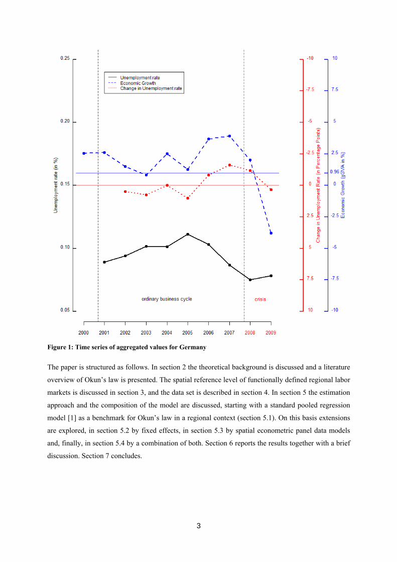
changes in the unemployment rate were observed. In figure 1 the national aggregated time series for
values of the unemployment rate (black line), the change in unemployment rate (dotted red line), and
the economic growth (blue dashed line) are shown for Germany. Up to 2008 the lines for changes in
the unemployment rate and economic growth are more or less concurrent with each other, with a
spread of one to two percentage points, but in 2008 this parallel run is interrupted. The question arises
as to whether this indicates decoupling effects. Nevertheless, there was a period of economic boom
alongside with a vigorous recovery of the labor market before the crisis.
This study examines the exceptional response of the German labor market to an economic downturn in
2008, using a disaggregated regional analysis approach to address the regional heterogeneity of the
German labor market. Another question considered is how far regional economic growth matters in
comparison to national macroeconomic growth developments. Hence the research question is specified
in a regional context, by asking if regional economic growth is related to regional labor market
development. The objective of this paper is to see whether Okun’s law can be confirmed as a rule of
thumb for labor market response to variations in regional economic growth. Identifying whether and to
what extent economic growth is a driving force of regional labor market development, is important for
economic and regional policy and a crucial factor in labor market analysis (Elhorst, 2003). An
estimation strategy is applied, starting with the simplest model and expanding it gradually to more
complex ones. The analysis is based on functionally defined regional markets and thereby accounts for
systematic spatial dependency with a non-parametric approach, but will also use parametric modeling
to take further non-systematic spatial effects and dynamic effects into account, utilizing spatial
econometric panel data models.
3
Figure 1: Time series of aggregated values for Germany
The paper is structured as follows. In section 2 the theoretical background is discussed and a literature
overview of Okun’s law is presented. The spatial reference level of functionally defined regional labor
markets is discussed in section 3, and the data set is described in section 4. In section 5 the estimation
approach and the composition of the model are discussed, starting with a standard pooled regression
model [1] as a benchmark for Okun’s law in a regional context (section 5.1). On this basis extensions
are explored, in section 5.2 by fixed effects, in section 5.3 by spatial econometric panel data models
and, finally, in section 5.4 by a combination of both. Section 6 reports the results together with a brief
discussion. Section 7 concludes.
4
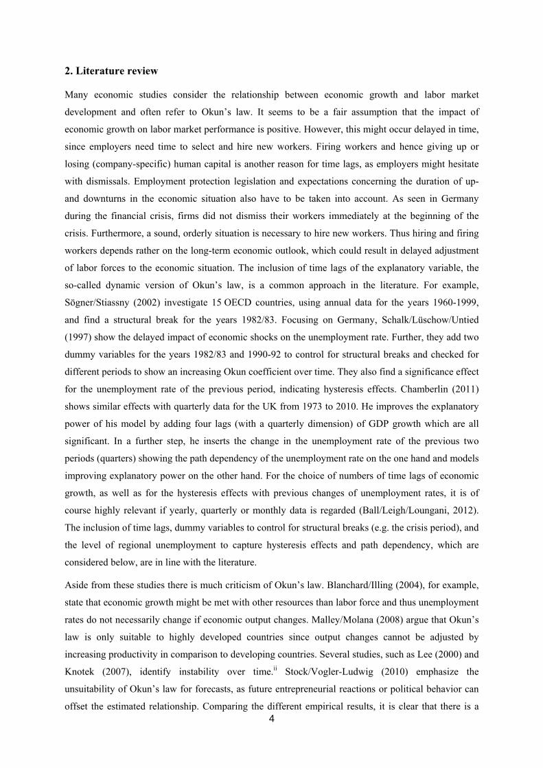
2. Literature review
Many economic studies consider the relationship between economic growth and labor market
development and often refer to Okun’s law. It seems to be a fair assumption that the impact of
economic growth on labor market performance is positive. However, this might occur delayed in time,
since employers need time to select and hire new workers. Firing workers and hence giving up or
losing (company-specific) human capital is another reason for time lags, as employers might hesitate
with dismissals. Employment protection legislation and expectations concerning the duration of up-
and downturns in the economic situation also have to be taken into account. As seen in Germany
during the financial crisis, firms did not dismiss their workers immediately at the beginning of the
crisis. Furthermore, a sound, orderly situation is necessary to hire new workers. Thus hiring and firing
workers depends rather on the long-term economic outlook, which could result in delayed adjustment
of labor forces to the economic situation. The inclusion of time lags of the explanatory variable, the
so-called dynamic version of Okun’s law, is a common approach in the literature. For example,
Sögner/Stiassny (2002) investigate 15 OECD countries, using annual data for the years 1960-1999,
and find a structural break for the years 1982/83. Focusing on Germany, Schalk/Lüschow/Untied
(1997) show the delayed impact of economic shocks on the unemployment rate. Further, they add two
dummy variables for the years 1982/83 and 1990-92 to control for structural breaks and checked for
different periods to show an increasing Okun coefficient over time. They also find a significance effect
for the unemployment rate of the previous period, indicating hysteresis effects. Chamberlin (2011)
shows similar effects with quarterly data for the UK from 1973 to 2010. He improves the explanatory
power of his model by adding four lags (with a quarterly dimension) of GDP growth which are all
significant. In a further step, he inserts the change in the unemployment rate of the previous two
periods (quarters) showing the path dependency of the unemployment rate on the one hand and models
improving explanatory power on the other hand. For the choice of numbers of time lags of economic
growth, as well as for the hysteresis effects with previous changes of unemployment rates, it is of
course highly relevant if yearly, quarterly or monthly data is regarded (Ball/Leigh/Loungani, 2012).
The inclusion of time lags, dummy variables to control for structural breaks (e.g. the crisis period), and
the level of regional unemployment to capture hysteresis effects and path dependency, which are
considered below, are in line with the literature.
Aside from these studies there is much criticism of Okun’s law. Blanchard/Illing (2004), for example,
state that economic growth might be met with other resources than labor force and thus unemployment
rates do not necessarily change if economic output changes. Malley/Molana (2008) argue that Okun’s
law is only suitable to highly developed countries since output changes cannot be adjusted by
increasing productivity in comparison to developing countries. Several studies, such as Lee (2000) and
Knotek (2007), identify instability over time.ii Stock/Vogler-Ludwig (2010) emphasize the
unsuitability of Okun’s law for forecasts, as future entrepreneurial reactions or political behavior can
offset the estimated relationship. Comparing the different empirical results, it is clear that there is a
5
high sensitivity regarding the chosen model specification, time periods and variables.iii Nevertheless,
the negative relationship between the unemployment rate and economic growth occurs in most
analyses. Pierdzioch/Rülke/Stadtmann (2012) identify Okun’s law as having high relevance for
professional economic forecasts, as forecasts of output growth and unemployment rates are consistent
with this macroeconomic model. Therefore Okun’s law as a rule of thumb is still applicable
(Perugini/Signorelli, 2005; Ball/Leigh/Loungani, 2012) and informative for policy-makers (IMF,
2012). Thus it is indispensable to scrutinize this relationship and to identify diverse interdependencies.
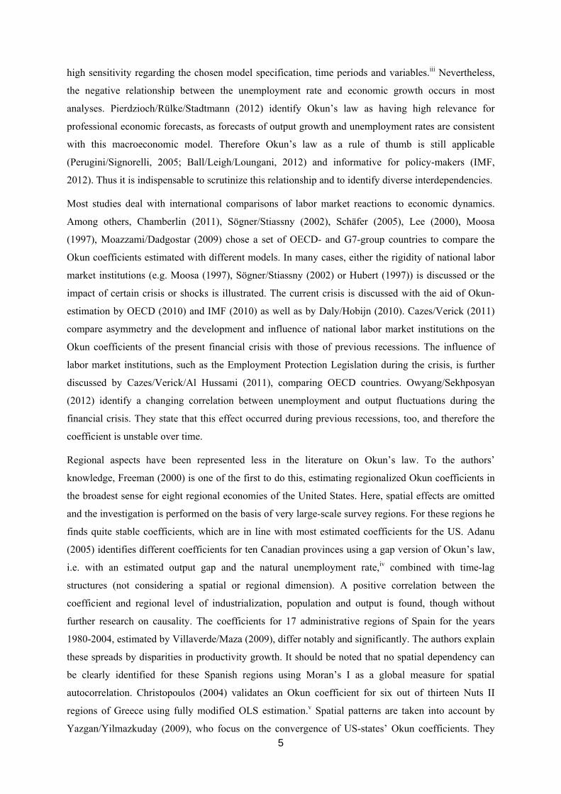
Most studies deal with international comparisons of labor market reactions to economic dynamics.
Among others, Chamberlin (2011), Sögner/Stiassny (2002), Schäfer (2005), Lee (2000), Moosa
(1997), Moazzami/Dadgostar (2009) chose a set of OECD- and G7-group countries to compare the
Okun coefficients estimated with different models. In many cases, either the rigidity of national labor
market institutions (e.g. Moosa (1997), Sögner/Stiassny (2002) or Hubert (1997)) is discussed or the
impact of certain crisis or shocks is illustrated. The current crisis is discussed with the aid of Okun-
estimation by OECD (2010) and IMF (2010) as well as by Daly/Hobijn (2010). Cazes/Verick (2011)
compare asymmetry and the development and influence of national labor market institutions on the
Okun coefficients of the present financial crisis with those of previous recessions. The influence of
labor market institutions, such as the Employment Protection Legislation during the crisis, is further
discussed by Cazes/Verick/Al Hussami (2011), comparing OECD countries. Owyang/Sekhposyan
(2012) identify a changing correlation between unemployment and output fluctuations during the
financial crisis. They state that this effect occurred during previous recessions, too, and therefore the
coefficient is unstable over time.
Regional aspects have been represented less in the literature on Okun’s law. To the authors’
knowledge, Freeman (2000) is one of the first to do this, estimating regionalized Okun coefficients in
the broadest sense for eight regional economies of the United States. Here, spatial effects are omitted
and the investigation is performed on the basis of very large-scale survey regions. For these regions he
finds quite stable coefficients, which are in line with most estimated coefficients for the US. Adanu
(2005) identifies different coefficients for ten Canadian provinces using a gap version of Okun’s law,
i.e. with an estimated output gap and the natural unemployment rate,iv combined with time-lag
structures (not considering a spatial or regional dimension). A positive correlation between the
coefficient and regional level of industrialization, population and output is found, though without
further research on causality. The coefficients for 17 administrative regions of Spain for the years
1980-2004, estimated by Villaverde/Maza (2009), differ notably and significantly. The authors explain
these spreads by disparities in productivity growth. It should be noted that no spatial dependency can
be clearly identified for these Spanish regions using Moran’s I as a global measure for spatial
autocorrelation. Christopoulos (2004) validates an Okun coefficient for six out of thirteen Nuts II
regions of Greece using fully modified OLS estimation.v Spatial patterns are taken into account by
Yazgan/Yilmazkuday (2009), who focus on the convergence of US-states’ Okun coefficients. They
6
use a geographically weighted regression for their first-difference approach, weighting regional output
by the distance of the location of production, to implement cross-country interactions.
Kangasharju/Pehkonen (2001) use a combination of regional, sectoral and time-effects in their first-
difference and dynamic approach for the Finnish labor market to identify the employment-output
relation between different regions. They find sectoral structure as one possible explanation.vi
A combination of institutional and regional influence of the unemployment intensity on economic
growth is analyzed by Herwartz/Niebuhr (2011). They control for institutional settings such as the
EPL (Employment Protection Legislation) on NUTS 2 regions in the EU-15. They also consider
interaction among neighboring labor markets, as well as the sectoral specialization and employment
density of regions. They find significant influence of all of these determinants, stressing the
persistence of regional disparities which cannot be directly influenced by labor market policies.
Kangasharku/Tavéra/Nijkamp (2011) also account for spatial dependencies in their survey as they use
a hidden cointegration approach for their estimation of the Okun coefficients. One special feature of
this analysis is the usage of functional delineated Finnish labor market regions. Similar to the approach
that will be used here, they deal with travel-to-work areas as regional labor markets. This is also done
by Kosfeld/Dreger (2005) for Germany. Their estimation approach is a spatial seemingly unrelated
regression, and both studies show that unemployment thresholds estimated without regarding spatial
effects are notably overestimated. The necessity of taking spatial interaction into account is also
shown by Niebuhr (2003) who identifies significant spatial dependencies between regional labor
markets in Europe.
In the present paper, we will include the aforementioned necessity of considering dynamic aspects in
the form of time lagsvii, as well as spatial effects, by testing, inter alia, regional individual fixed
effects, spatially lagged explanatory variables and spatial error processes in the disturbances – all in
combination with the use of functional delineated economic market areas as study areas. These
functional markets will lower spillover effects and strengthen the explanatory power of our
estimations. In comparison with the literature, our data set consists of a rather short period covering
2002 to 2009, but a high number of observation units with 110 regional markets.
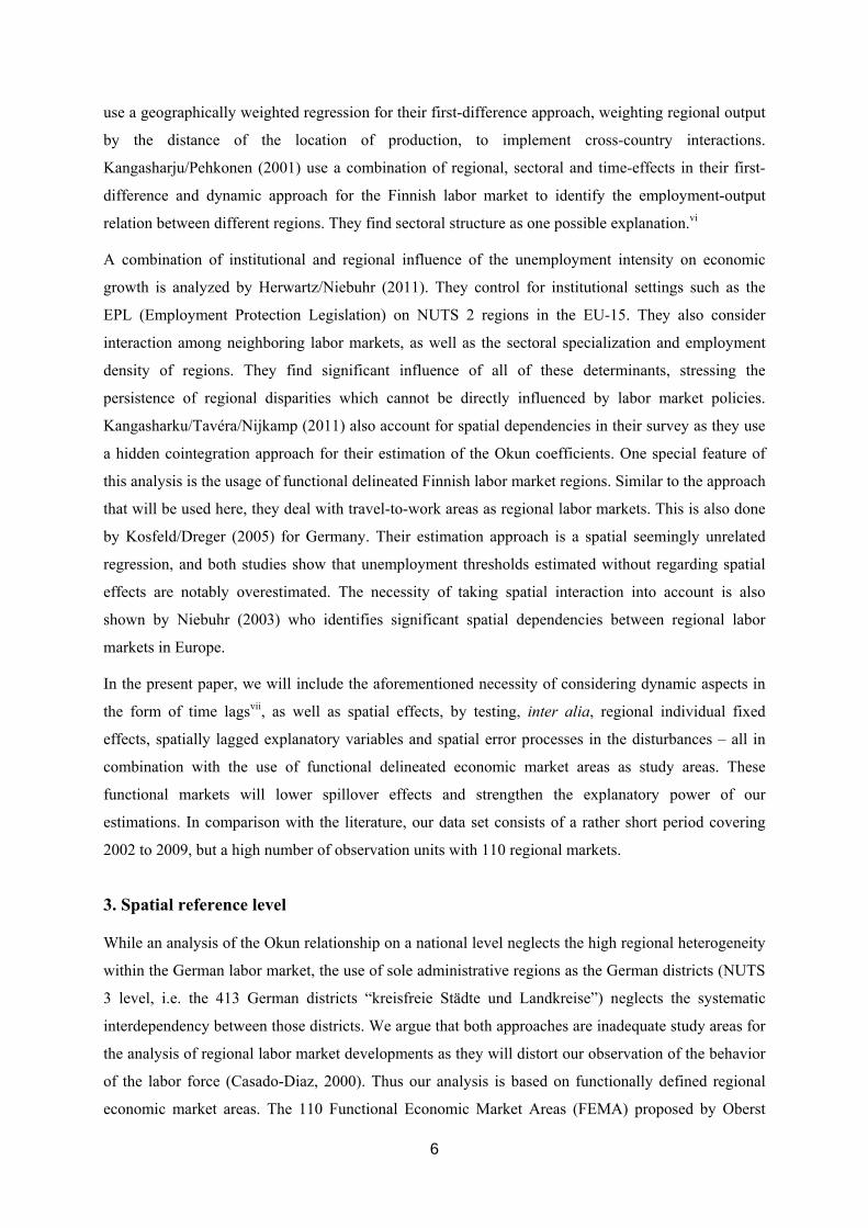
3. Spatial reference level
While an analysis of the Okun relationship on a national level neglects the high regional heterogeneity
within the German labor market, the use of sole administrative regions as the German districts (NUTS
3 level, i.e. the 413 German districts “kreisfreie Städte und Landkreise”) neglects the systematic
interdependency between those districts. We argue that both approaches are inadequate study areas for
the analysis of regional labor market developments as they will distort our observation of the behavior
of the labor force (Casado-Diaz, 2000). Thus our analysis is based on functionally defined regional
economic market areas. The 110 Functional Economic Market Areas (FEMA) proposed by Oberst
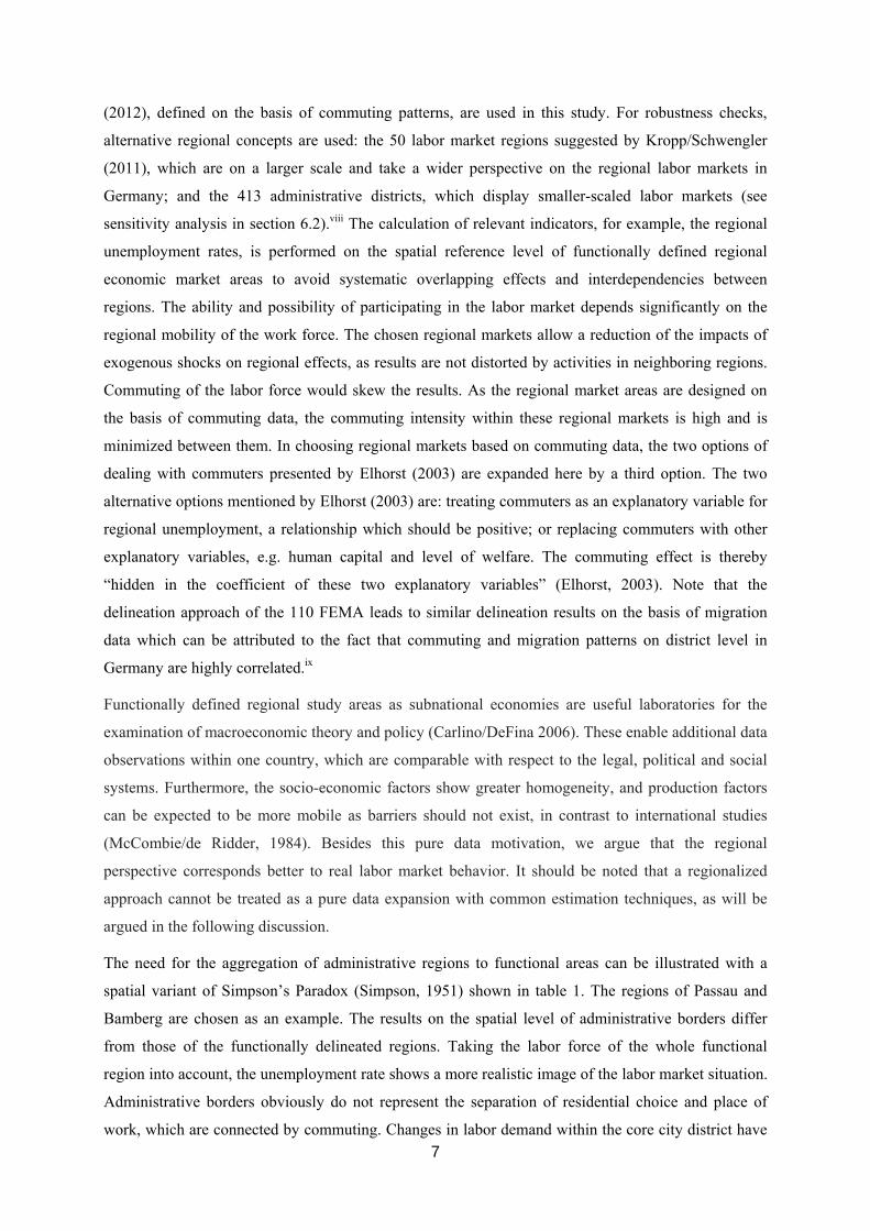
7
(2012), defined on the basis of commuting patterns, are used in this study. For robustness checks,
alternative regional concepts are used: the 50 labor market regions suggested by Kropp/Schwengler
(2011), which are on a larger scale and take a wider perspective on the regional labor markets in
Germany; and the 413 administrative districts, which display smaller-scaled labor markets (see
sensitivity analysis in section 6.2).viii The calculation of relevant indicators, for example, the regional
unemployment rates, is performed on the spatial reference level of functionally defined regional
economic market areas to avoid systematic overlapping effects and interdependencies between
regions. The ability and possibility of participating in the labor market depends significantly on the
regional mobility of the work force. The chosen regional markets allow a reduction of the impacts of
exogenous shocks on regional effects, as results are not distorted by activities in neighboring regions.
Commuting of the labor force would skew the results. As the regional market areas are designed on
the basis of commuting data, the commuting intensity within these regional markets is high and is
minimized between them. In choosing regional markets based on commuting data, the two options of
dealing with commuters presented by Elhorst (2003) are expanded here by a third option. The two
alternative options mentioned by Elhorst (2003) are: treating commuters as an explanatory variable for
regional unemployment, a relationship which should be positive; or replacing commuters with other
explanatory variables, e.g. human capital and level of welfare. The commuting effect is thereby
“hidden in the coefficient of these two explanatory variables” (Elhorst, 2003). Note that the
delineation approach of the 110 FEMA leads to similar delineation results on the basis of migration
data which can be attributed to the fact that commuting and migration patterns on district level in
Germany are highly correlated.ix
Functionally defined regional study areas as subnational economies are useful laboratories for the
examination of macroeconomic theory and policy (Carlino/DeFina 2006). These enable additional data
observations within one country, which are comparable with respect to the legal, political and social
systems. Furthermore, the socio-economic factors show greater homogeneity, and production factors
can be expected to be more mobile as barriers should not exist, in contrast to international studies
(McCombie/de Ridder, 1984). Besides this pure data motivation, we argue that the regional
perspective corresponds better to real labor market behavior. It should be noted that a regionalized
approach cannot be treated as a pure data expansion with common estimation techniques, as will be
argued in the following discussion.
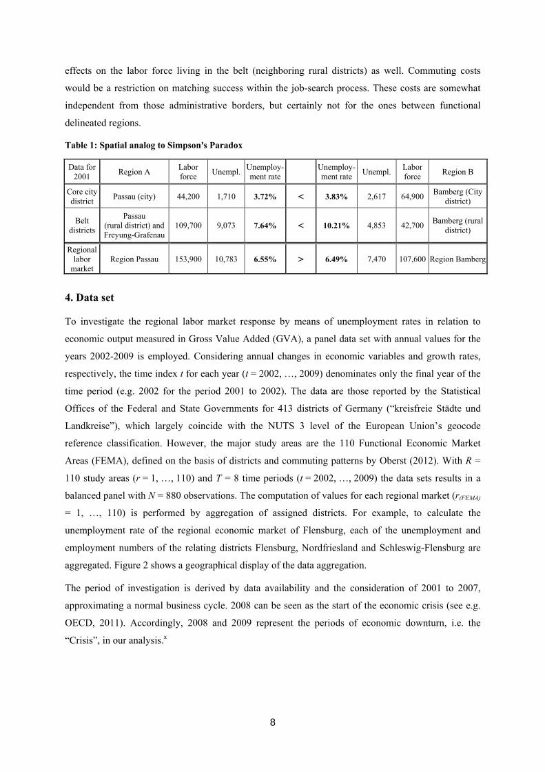
The need for the aggregation of administrative regions to functional areas can be illustrated with a
spatial variant of Simpson’s Paradox (Simpson, 1951) shown in table 1. The regions of Passau and
Bamberg are chosen as an example. The results on the spatial level of administrative borders differ
from those of the functionally delineated regions. Taking the labor force of the whole functional
region into account, the unemployment rate shows a more realistic image of the labor market situation.
Administrative borders obviously do not represent the separation of residential choice and place of
work, which are connected by commuting. Changes in labor demand within the core city district have
8
effects on the labor force living in the belt (neighboring rural districts) as well. Commuting costs
would be a restriction on matching success within the job-search process. These costs are somewhat
independent from those administrative borders, but certainly not for the ones between functional
delineated regions.
Table 1: Spatial analog to Simpson's Paradox
4. Data set
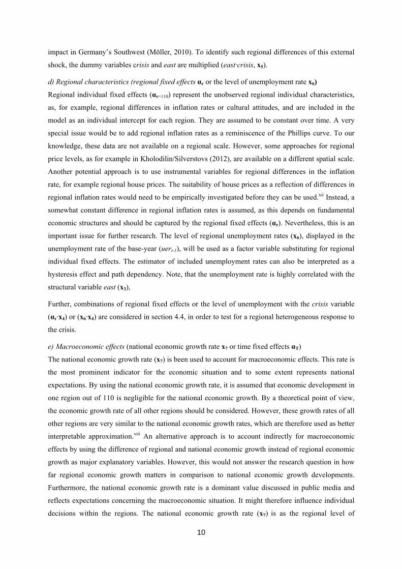
To investigate the regional labor market response by means of unemployment rates in relation to
economic output measured in Gross Value Added (GVA), a panel data set with annual values for the
years 2002-2009 is employed. Considering annual changes in economic variables and growth rates,
respectively, the time index t for each year (t = 2002, …, 2009) denominates only the final year of the
time period (e.g. 2002 for the period 2001 to 2002). The data are those reported by the Statistical
Offices of the Federal and State Governments for 413 districts of Germany (“kreisfreie Städte und
Landkreise”), which largely coincide with the NUTS 3 level of the European Union’s geocode
reference classification. However, the major study areas are the 110 Functional Economic Market
Areas (FEMA), defined on the basis of districts and commuting patterns by Oberst (2012). With R =
110 study areas (r = 1, …, 110) and T = 8 time periods (t = 2002, …, 2009) the data sets results in a
balanced panel with N = 880 observations. The computation of values for each regional market (r(FEMA)
= 1, …, 110) is performed by aggregation of assigned districts. For example, to calculate the
unemployment rate of the regional economic market of Flensburg, each of the unemployment and
employment numbers of the relating districts Flensburg, Nordfriesland and Schleswig-Flensburg are
aggregated. Figure 2 shows a geographical display of the data aggregation.
The period of investigation is derived by data availability and the consideration of 2001 to 2007,
approximating a normal business cycle. 2008 can be seen as the start of the economic crisis (see e.g.
OECD, 2011). Accordingly, 2008 and 2009 represent the periods of economic downturn, i.e. the
“Crisis”, in our analysis.x
Data for 2001
Region A Labor force
Unempl.Unemploy-ment rate
Unemploy-ment rate
Unempl. Labor force
Region B
Core city district
Passau (city) 44,200 1,710 3.72% < 3.83% 2,617 64,900 Bamberg (City
district)
Belt districts
Passau (rural district) and Freyung-Grafenau
109,700 9,073 7.64% < 10.21% 4,853 42,700 Bamberg (rural
district)
Regional labor
market Region Passau 153,900 10,783 6.55% > 6.49% 7,470 107,600 Region Bamberg
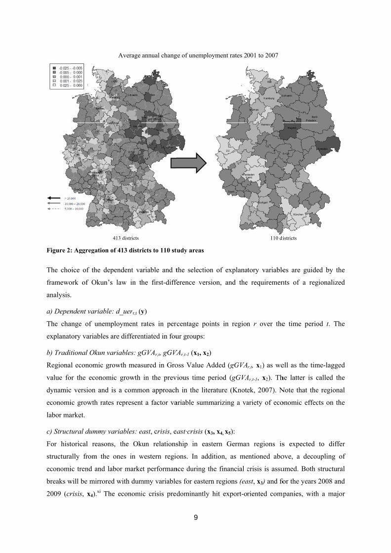
Figure 2
The cho
framewo
analysis.
a) Depen
The cha
explanat
b) Tradi
Regiona
value fo
dynamic
economi
labor ma
c) Struct
For hist
structura
economi
breaks w
2009 (cr
: Aggregation
oice of the d
ork of Okun
.
ndent variab
ange of unem
tory variable
tional Okun
al economic g
or the econo
c version and
ic growth rat
arket.
tural dummy
torical reaso
ally from th
ic trend and
will be mirror
risis, x4).xi T
n of 413 distr
dependent va
n’s law in t
ble: d_uerr,t (y
mployment r
s are differen
variables: g
growth meas
mic growth
d is a comm
tes represent
y variables: e
ons, the Ok
he ones in w
labor marke
red with dum
The economi
Average
413 districts
ricts to 110 stu
ariable and t
he first-diffe
y)
rates in perc
ntiated in fou
gGVAr,t, gGVA
sured in Gro
in the prev
mon approach
t a factor va
east, crisis, e
kun relations
western regio
et performan
mmy variable
ic crisis pred
annual chang
9
udy areas
the selection
ference versi
centage poin
ur groups:
VAr,t-1 (x1, x2)
oss Value Ad
vious time pe
h in the liter
ariable summ
ast·crisis (x3
ship in east
ons. In addi
nce during th
es for eastern
dominantly
ge of unemploy
n of explana
ion, and the
nts in region
dded (gGVA
eriod (gGVA
rature (Knote
marizing a va
3, x4, x5):
tern German
ition, as me
he financial c
n regions (ea
hit export-o
yment rates 2
tory variable
e requiremen
n r over the
r,t, x1) as we
Ar,t-1, x2). Th
ek, 2007). N
ariety of eco
n regions is
entioned abo
crisis is assu
ast, x3) and fo
riented comp
001 to 2007
110 di
es are guide
nts of a reg
e time perio
ell as the tim
he latter is c
Note that the
onomic effec
s expected
ove, a decou
umed. Both
for the years
mpanies, with
istricts
ed by the
gionalized
od t. The
me-lagged
called the
e regional
cts on the
to differ
upling of
structural
2008 and
h a major
10
impact in Germany’s Southwest (Möller, 2010). To identify such regional differences of this external
shock, the dummy variables crisis and east are multiplied (east·crisis, x5).
d) Regional characteristics (regional fixed effects αr or the level of unemployment rate x6)
Regional individual fixed effects (αr=110) represent the unobserved regional individual characteristics,
as, for example, regional differences in inflation rates or cultural attitudes, and are included in the
model as an individual intercept for each region. They are assumed to be constant over time. A very
special issue would be to add regional inflation rates as a reminiscence of the Phillips curve. To our
knowledge, these data are not available on a regional scale. However, some approaches for regional
price levels, as for example in Kholodilin/Silverstovs (2012), are available on a different spatial scale.
Another potential approach is to use instrumental variables for regional differences in the inflation
rate, for example regional house prices. The suitability of house prices as a reflection of differences in
regional inflation rates would need to be empirically investigated before they can be used.xii Instead, a
somewhat constant difference in regional inflation rates is assumed, as this depends on fundamental
economic structures and should be captured by the regional fixed effects (αr). Nevertheless, this is an
important issue for further research. The level of regional unemployment rates (x6), displayed in the
unemployment rate of the base-year (uert-1), will be used as a factor variable substituting for regional
individual fixed effects. The estimator of included unemployment rates can also be interpreted as a
hysteresis effect and path dependency. Note, that the unemployment rate is highly correlated with the
structural variable east (x3),
Further, combinations of regional fixed effects or the level of unemployment with the crisis variable
(αr·x4) or (x6·x4) are considered in section 4.4, in order to test for a regional heterogeneous response to
the crisis.
e) Macroeconomic effects (national economic growth rate x7 or time fixed effects αT)
The national economic growth rate (x7) is been used to account for macroeconomic effects. This rate is
the most prominent indicator for the economic situation and to some extent represents national
expectations. By using the national economic growth rate, it is assumed that economic development in
one region out of 110 is negligible for the national economic growth. By a theoretical point of view,
the economic growth rate of all other regions should be considered. However, these growth rates of all
other regions are very similar to the national economic growth rates, which are therefore used as better
interpretable approximation.xiii An alternative approach is to account indirectly for macroeconomic
effects by using the difference of regional and national economic growth instead of regional economic
growth as major explanatory variables. However, this would not answer the research question in how
far regional economic growth matters in comparison to national economic growth developments.
Furthermore, the national economic growth rate is a dominant value discussed in public media and
reflects expectations concerning the macroeconomic situation. It might therefore influence individual
decisions within the regions. The national economic growth rate (x7) is as the regional level of
11
unemployment rates (x6) included in the set of explanatory variables in X. An alternative to control for
macroeconomic effects is the implementation of time fixed effects (αT), representing annual specific
effects, which are equal for all regions, and which are estimated as an individual intercept for each
year. However, time fixed effects overlay highly with both the national economic growth rate and the
dummy variable for the crisis. These are therefore omitted in most of the results presented later, and
the focus lays on the directly economically interpretable national economic growth rates. For results
on estimations with pure time fixed effects, see Appendix 2.
f) Spatial parameters (WX, and/or λWε)
Intuitively, spatially lagged explanatory variables (WX) can be interpreted as the weighted average
values from neighboring regions. To calculate these values, the assumption of the spatial weight
matrix (W), representing the structure of spatial connectivity between regions, is decisive. The spatial
weights included in the matrix are usually interpreted as functions of economic or geographic
proximity between spatial units. Since it has to be defined a priori, the specific form of W is probably
the strongest assumption of the spatial analysis. Yet economic theory provides little guidance on
specifying these weights. In order to examine the robustness of the results with respect to the form of
W, three different weight matrices are employed (see section 6.2). The reference matrix, for which
results are reported in the following sections, is a standard row-stochastic first-order queen-contiguity
matrix.xiv ε is a disturbance term governed by a spatial autoregressive process (Wε), with λ as the
associated scalar parameter. See section 5.3 for a more detailed description of spatial parameters.
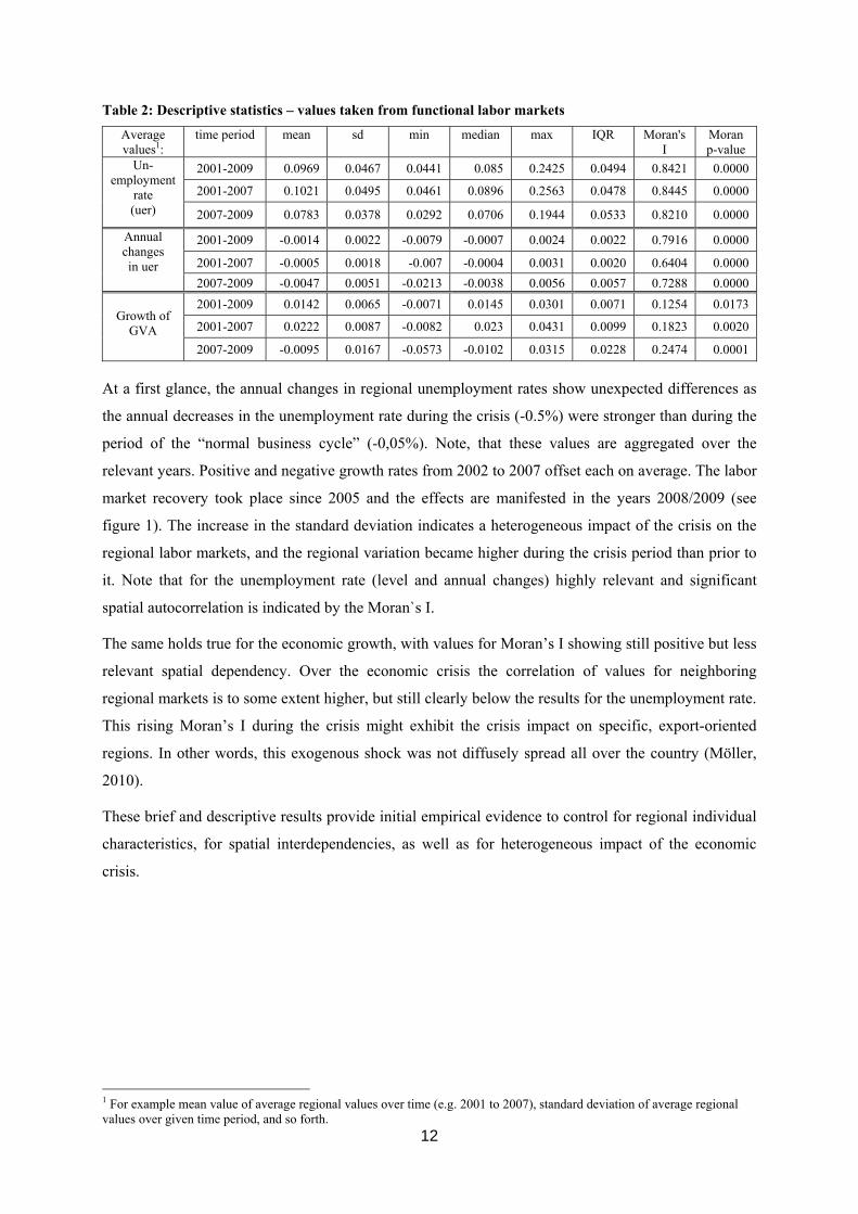
Some descriptive statistics for average regional unemployment rates, the average annual change in
unemployment rates, and the economic growth measured in GVA are documented in table 2. For three
different time periods average values for the regional mean, standard deviation (sd), minimum, median
and maximum values, the interquartile range (IQR, 0.75-quantile – 0.25-quantile) and the Moran’s I
statistics (Cliff/Ord, 1981)xv as a global measure for spatial autocorrelation are reported.
The average regional unemployment rate during the time of the normal business cycle, at 10.2%,
exceeds the value of the crisis period, which is 7.8%. This mirrors the dynamics that took place in the
years before 2008 when there was a strong recovery of the German labor market – and the transition
from the “sick man of the euro” (The Economist) at the beginning of the century, via Germanys Jobs
Miracle (e.g. Krugman, 2009) to Europe’s Engine and Model of success (expressions refer to articles
in The Economist, June 3, 1999, March 11, 2010, and April 17, 2012, as well as Krugman, November
12, 2009 in The New York Times). The changes in regional variation in unemployment rates are
ambiguous: while the standard deviation is lower for the time period 2007-2009, the interquartile
range is higher. The improvement in the labor market is shown for the best performer (minimum) as
well as for the low-performing, but the discrepancy within the German labor market remains high with
a range of regional unemployment rates from 3.8% to 19.4%.
12
Table 2: Descriptive statistics – values taken from functional labor markets
Average values1:
time period mean
sd min median max IQR Moran's I
Moran p-value
Un-employment
rate (uer)
2001-2009 0.0969 0.0467 0.0441 0.085 0.2425 0.0494 0.8421 0.0000
2001-2007 0.1021 0.0495 0.0461 0.0896 0.2563 0.0478 0.8445 0.0000
2007-2009 0.0783 0.0378 0.0292 0.0706 0.1944 0.0533 0.8210 0.0000
Annual changes in uer
2001-2009 -0.0014 0.0022 -0.0079 -0.0007 0.0024 0.0022 0.7916 0.0000
2001-2007 -0.0005 0.0018 -0.007 -0.0004 0.0031 0.0020 0.6404 0.0000
2007-2009 -0.0047 0.0051 -0.0213 -0.0038 0.0056 0.0057 0.7288 0.0000
Growth of GVA
2001-2009 0.0142 0.0065 -0.0071 0.0145 0.0301 0.0071 0.1254 0.0173
2001-2007 0.0222 0.0087 -0.0082 0.023 0.0431 0.0099 0.1823 0.0020
2007-2009 -0.0095 0.0167 -0.0573 -0.0102 0.0315 0.0228 0.2474 0.0001
At a first glance, the annual changes in regional unemployment rates show unexpected differences as
the annual decreases in the unemployment rate during the crisis (-0.5%) were stronger than during the
period of the “normal business cycle” (-0,05%). Note, that these values are aggregated over the
relevant years. Positive and negative growth rates from 2002 to 2007 offset each on average. The labor
market recovery took place since 2005 and the effects are manifested in the years 2008/2009 (see
figure 1). The increase in the standard deviation indicates a heterogeneous impact of the crisis on the
regional labor markets, and the regional variation became higher during the crisis period than prior to
it. Note that for the unemployment rate (level and annual changes) highly relevant and significant
spatial autocorrelation is indicated by the Moran`s I.
The same holds true for the economic growth, with values for Moran’s I showing still positive but less
relevant spatial dependency. Over the economic crisis the correlation of values for neighboring
regional markets is to some extent higher, but still clearly below the results for the unemployment rate.
This rising Moran’s I during the crisis might exhibit the crisis impact on specific, export-oriented
regions. In other words, this exogenous shock was not diffusely spread all over the country (Möller,
2010).
These brief and descriptive results provide initial empirical evidence to control for regional individual
characteristics, for spatial interdependencies, as well as for heterogeneous impact of the economic
crisis.
1 For example mean value of average regional values over time (e.g. 2001 to 2007), standard deviation of average regional values over given time period, and so forth.
13
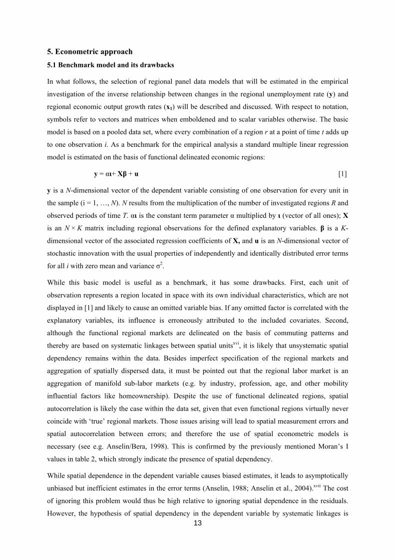
5. Econometric approach
5.1 Benchmark model and its drawbacks
In what follows, the selection of regional panel data models that will be estimated in the empirical
investigation of the inverse relationship between changes in the regional unemployment rate (y) and
regional economic output growth rates (x1) will be described and discussed. With respect to notation,
symbols refer to vectors and matrices when emboldened and to scalar variables otherwise. The basic
model is based on a pooled data set, where every combination of a region r at a point of time t adds up
to one observation i. As a benchmark for the empirical analysis a standard multiple linear regression
model is estimated on the basis of functional delineated economic regions:
y = αι+ Xβ + u [1]
y is a N-dimensional vector of the dependent variable consisting of one observation for every unit in
the sample (i = 1, …, N). N results from the multiplication of the number of investigated regions R and
observed periods of time T. αι is the constant term parameter α multiplied by ι (vector of all ones); X
is an N × K matrix including regional observations for the defined explanatory variables. β is a K-
dimensional vector of the associated regression coefficients of X, and u is an N-dimensional vector of
stochastic innovation with the usual properties of independently and identically distributed error terms
for all i with zero mean and variance σ2.
While this basic model is useful as a benchmark, it has some drawbacks. First, each unit of
observation represents a region located in space with its own individual characteristics, which are not
displayed in [1] and likely to cause an omitted variable bias. If any omitted factor is correlated with the
explanatory variables, its influence is erroneously attributed to the included covariates. Second,
although the functional regional markets are delineated on the basis of commuting patterns and
thereby are based on systematic linkages between spatial unitsxvi, it is likely that unsystematic spatial
dependency remains within the data. Besides imperfect specification of the regional markets and
aggregation of spatially dispersed data, it must be pointed out that the regional labor market is an
aggregation of manifold sub-labor markets (e.g. by industry, profession, age, and other mobility
influential factors like homeownership). Despite the use of functional delineated regions, spatial
autocorrelation is likely the case within the data set, given that even functional regions virtually never
coincide with ‘true’ regional markets. Those issues arising will lead to spatial measurement errors and
spatial autocorrelation between errors; and therefore the use of spatial econometric models is
necessary (see e.g. Anselin/Bera, 1998). This is confirmed by the previously mentioned Moran’s I
values in table 2, which strongly indicate the presence of spatial dependency.
While spatial dependence in the dependent variable causes biased estimates, it leads to asymptotically
unbiased but inefficient estimates in the error terms (Anselin, 1988; Anselin et al., 2004).xvii The cost
of ignoring this problem would thus be high relative to ignoring spatial dependence in the residuals.
However, the hypothesis of spatial dependency in the dependent variable by systematic linkages is
14
rejected here due to theoretical considerations, and it is assumed that the present spatial dependency is
caused by unsystematic linkages. Note that systematic spatial dependency is already captured by the
non-parametric approach of functionally defined regional markets.
The drawbacks of the benchmark model [1] will be addressed as follows. First, in section 5.2, the
implementation of fixed effects is discussed to control for different regional characteristics of the
regional labor markets as well as to control for macroeconomic effects. Second, in section 5.3, the
model is estimated in spatial econometric settings, with the Spatial Durbin Error Model (SDEM) as the
preferred approach due to the assumed simultaneous presence of omitted variable bias and spatial
dependency caused by unsystematic linkages. Finally, a potential combination of both approaches is
considered in section 5.4.
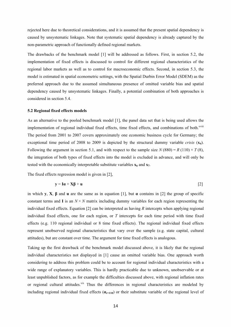
5.2 Regional fixed effects models
As an alternative to the pooled benchmark model [1], the panel data set that is being used allows the
implementation of regional individual fixed effects, time fixed effects, and combinations of both.xviii
The period from 2001 to 2007 covers approximately one economic business cycle for Germany; the
exceptional time period of 2008 to 2009 is depicted by the structural dummy variable crisis (x4).
Following the argument in section 5.1, and with respect to the sample size N (880) = R (110) × T (8),
the integration of both types of fixed effects into the model is excluded in advance, and will only be
tested with the economically interpretable substitute variables x6 and x7.
The fixed effects regression model is given in [2],
y = Ια + Xβ + u [2]
in which y, X, β and u are the same as in equation [1], but α contains in [2] the group of specific
constant terms and Ι is an N × N matrix including dummy variables for each region representing the
individual fixed effects. Equation [2] can be interpreted as having R intercepts when applying regional
individual fixed effects, one for each region, or T intercepts for each time period with time fixed
effects (e.g. 110 regional individual or 8 time fixed effects). The regional individual fixed effects
represent unobserved regional characteristics that vary over the sample (e.g. state capital, cultural
attitudes), but are constant over time. The argument for time fixed effects is analogous.
Taking up the first drawback of the benchmark model discussed above, it is likely that the regional
individual characteristics not displayed in [1] cause an omitted variable bias. One approach worth
considering to address this problem could be to account for regional individual characteristics with a
wide range of explanatory variables. This is hardly practicable due to unknown, unobservable or at
least unpublished factors, as for example the difficulties discussed above, with regional inflation rates
or regional cultural attitudes.xix Thus the differences in regional characteristics are modeled by
including regional individual fixed effects (αr=110) or their substitute variable of the regional level of
15
unemployment (x6). However, the explanation of differences in regional characteristics, as well as
finding and constructing suitable explanatory variables, is an important aspect for further research.
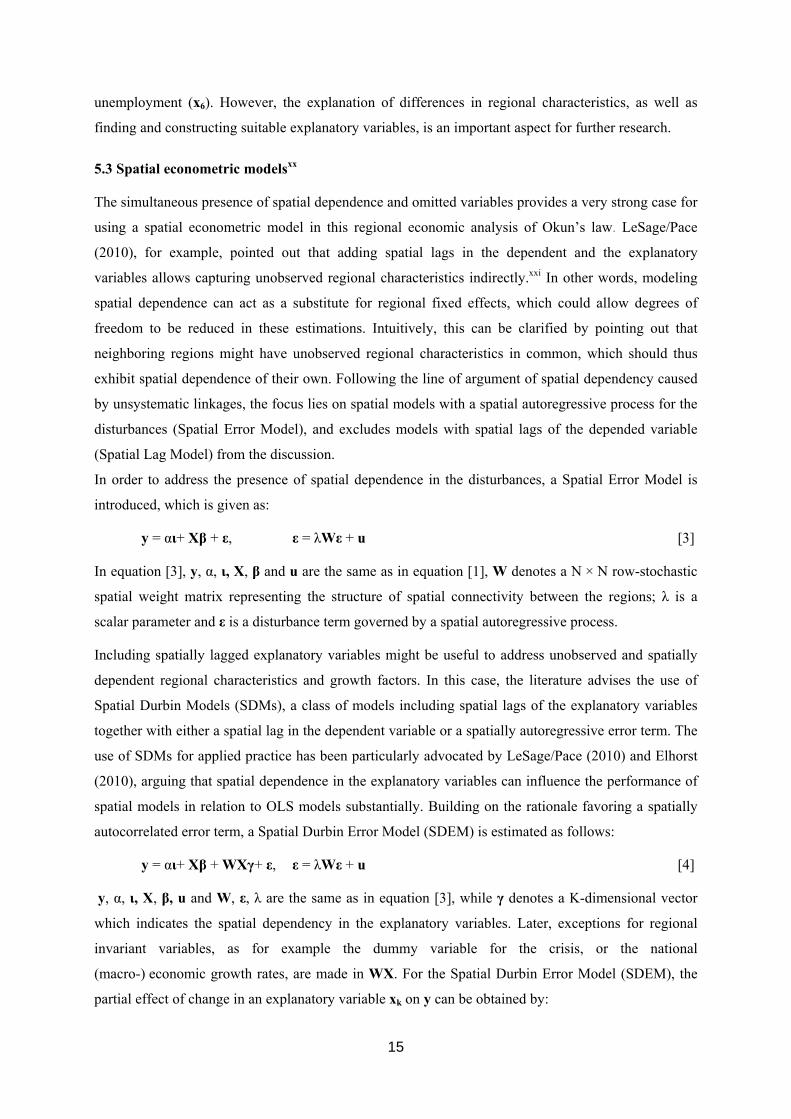
5.3 Spatial econometric modelsxx
The simultaneous presence of spatial dependence and omitted variables provides a very strong case for
using a spatial econometric model in this regional economic analysis of Okun’s law. LeSage/Pace
(2010), for example, pointed out that adding spatial lags in the dependent and the explanatory
variables allows capturing unobserved regional characteristics indirectly.xxi In other words, modeling
spatial dependence can act as a substitute for regional fixed effects, which could allow degrees of
freedom to be reduced in these estimations. Intuitively, this can be clarified by pointing out that
neighboring regions might have unobserved regional characteristics in common, which should thus
exhibit spatial dependence of their own. Following the line of argument of spatial dependency caused
by unsystematic linkages, the focus lies on spatial models with a spatial autoregressive process for the
disturbances (Spatial Error Model), and excludes models with spatial lags of the depended variable
(Spatial Lag Model) from the discussion.
In order to address the presence of spatial dependence in the disturbances, a Spatial Error Model is
introduced, which is given as:
y = αι+ Xβ + ε, ε = λWε + u [3]
In equation [3], y, α, ι, X, β and u are the same as in equation [1], W denotes a N × N row-stochastic
spatial weight matrix representing the structure of spatial connectivity between the regions; λ is a
scalar parameter and ε is a disturbance term governed by a spatial autoregressive process.
Including spatially lagged explanatory variables might be useful to address unobserved and spatially
dependent regional characteristics and growth factors. In this case, the literature advises the use of
Spatial Durbin Models (SDMs), a class of models including spatial lags of the explanatory variables
together with either a spatial lag in the dependent variable or a spatially autoregressive error term. The
use of SDMs for applied practice has been particularly advocated by LeSage/Pace (2010) and Elhorst
(2010), arguing that spatial dependence in the explanatory variables can influence the performance of
spatial models in relation to OLS models substantially. Building on the rationale favoring a spatially
autocorrelated error term, a Spatial Durbin Error Model (SDEM) is estimated as follows:
y = αι+ Xβ + WXγ+ ε, ε = λWε + u [4]
y, α, ι, X, β, u and W, ε, λ are the same as in equation [3], while γ denotes a K-dimensional vector
which indicates the spatial dependency in the explanatory variables. Later, exceptions for regional
invariant variables, as for example the dummy variable for the crisis, or the national
(macro-) economic growth rates, are made in WX. For the Spatial Durbin Error Model (SDEM), the
partial effect of change in an explanatory variable xk on y can be obtained by:
16
knknk
WIx
y
[5]
for all k, where Inβk measure the direct effect (within the regional market) and Wnyk the indirect effect
(cumulative neighboring effects). The β-coefficient can be interpreted as in common OLS-regression,
while Wnγk is the product of the spatial weight matrix and the considered spatial lag parameters γk and
includes the SDEM-typical local multiplier. The average row sum corresponds to the average
cumulative indirect effect (see Lerbs/Oberst, 2012). The possibility of this intuitive parameter
interpretation is another advantage of the SDEM in regard to spatial models, including spatial lags of
the dependent variable as the SDM.
5.4 Spatial econometric models with fixed effects
As derived from the previous discussion, it is important to account for regional individual
characteristics, macroeconomic effects, as well as spatial dependency. In general, the employed
regional panel data set allows for control of all of this. However, the main obstacles are
multicollinearity problems and sample size. Three variations of the Spatial Durbin Error Models
(SDEM) with regional fixed effects will be considered in the following discussion. The first model [6]
controls for regional heterogeneous characteristics and is a combination of the SDEM with regional
individual fixed effects, the second model [7] depicts only a regional heterogeneous response towards
the economic crisis with an interaction term of the dummy variable for the crisis (x4) and the matrix of
and the N × N matrix I (in analogy with the interaction of east·crisis, x5), but consists of an ordinary
intercept α [7]. Finally, the third model [8] is a combination of both, displaying both regional
heterogeneous characteristics and heterogeneous response to the crisis. A detailed description of
formulas is omitted here, since most terms are already described above.
y = αι+ Xβ + WXγ+ ε, ε = λWε + u [6]
y = αι+ Xβ + WXγ+ αι·x4τ + ε, ε = λWε + u [7]
y = αι+ Xβ + WXγ+ αι·x4τ + ε, ε = λWε + u [8]
While α in [6] and [8] contains the group of R specific constant terms for regional individual fixed
effects as described in section 5.2, α in [7] is the scalar parameter and constant term as in the
benchmark model [1]. αι·x4 displays the described regional heterogeneous response, with τ as the
vector of associated coefficients.
17
6. Empirical results
6.1 Empirical results for the reference level of 110 FEMA
All the models presented are estimated with a maximum likelihood procedurexxii and employed on the
aggregated regional panel data set for 110 functional delineated regional markets in Germany with
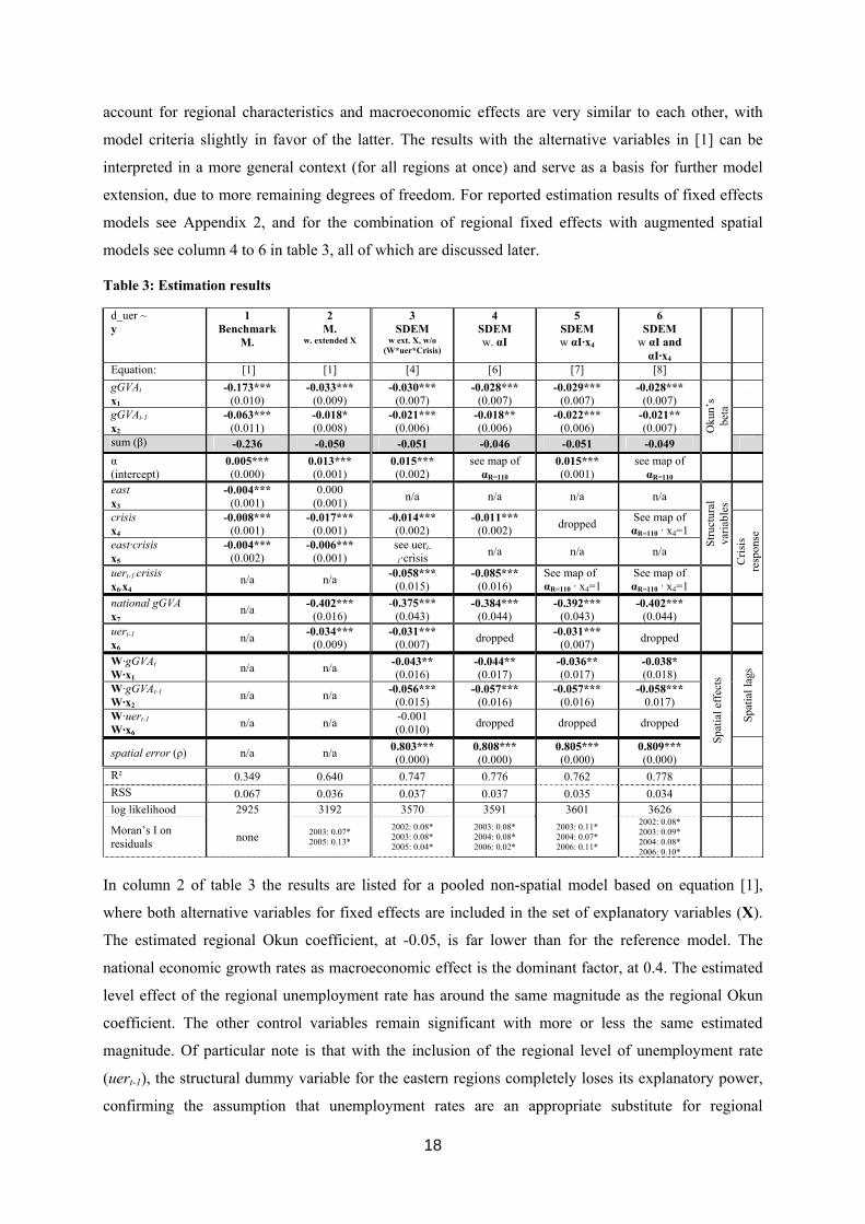
values for 2002 to 2009. The empirical results are summarized in table 3, where standard errors of
estimates are given in parentheses and the level of significance is indicated with *, **, and *** for
10%, 1%, and 0.1%-level. The R² and the log likelihood are used for model comparison. While R²
indicates the goodness of fit between estimated y and observed values for y, the log likelihood shows
the values of the log likelihood function at the optimum. The higher the log likelihood values, the
more likely the parameter. Subsequent to the presentation of empirical results, a sensitivity analysis for
alternative regional market definitions and spatial neighborhood criteria follows in section 6.2.
The discussion of the empirical results starts with the pooled and non-spatial Benchmark Model
specified in [1], the results of which are given in the 1st column of table 3 and serve as a reference
point for the analysis.xxiii The estimated Okun coefficient β1,2 (with consideration of timely lagged
effects, t, t-1) is -0.24. The resulting estimated regional growth thresholdxxiv is 2.3%, (for calculation of
these thresholds see Appendix 1). All included control variables are shown as significant with negative
signs, indicating lower growth thresholds for eastern regions (1.9%); for the time period of the
economic crisis (1.5%); and for eastern regions during the economic crisis (0.7%). This pooled model
implies the assumption that the same estimated coefficients and thus the Okun relationship is the same
for each region in each year (except for the differences controlled for with structural dummies). This
assumption of stability is questionable, as can be shown with theoretical arguments and empirical
testing (chow test).xxv
The standard way of accounting for regional characteristics with panel data is to add individual fixed
effects αr for each regional labor market, as in equation [2] with αr containing R=110 intercepts.
Alternatively, the level of regional unemployment x6 as a substitute for regional individual fixed
effects and as a proxy variable for different regional labor market situations is proposed. The
correlation coefficient between regional individual fixed effects and the level of unemployment rates
across different estimated models is sufficiently high, at 0.9 in non-spatial pooled models and about
0.74 in spatial models. Note that the level of unemployment rate is just one aspect of regional
attributes – albeit most likely the decisive one, and that a simultaneous estimation of both variables for
regional characteristics is not feasible due to the occurrence of multicollinearity problems. The same
holds true for the temporal dimension, where the national economic growth rate x7 and time fixed
effects αT are substitute variables. Note that time fixed effects need to be interpreted in a broader sense
because they also cover special annual effects (e.g. policy reforms such as Agenda 2010 by the
Schröder Government). However, the estimation results for a time fixed effects model [2], with αT
containing T=8 intercepts, and the reference model [1] including the proposed alternative variables to
18
account for regional characteristics and macroeconomic effects are very similar to each other, with
model criteria slightly in favor of the latter. The results with the alternative variables in [1] can be
interpreted in a more general context (for all regions at once) and serve as a basis for further model
extension, due to more remaining degrees of freedom. For reported estimation results of fixed effects
models see Appendix 2, and for the combination of regional fixed effects with augmented spatial
models see column 4 to 6 in table 3, all of which are discussed later.
Table 3: Estimation results
d_uer ~ y
1 Benchmark
M.
2 M.
w. extended X
3 SDEM
w ext. X, w/o (W*uer*Crisis)
4 SDEM w. αΙ
5 SDEM w αΙ·x4
6 SDEM
w αΙ and αΙ·x4
Equation: [1] [1] [4] [6] [7] [8]
gGVAt
x1 -0.173***
(0.010) -0.033***
(0.009) -0.030***
(0.007) -0.028***
(0.007) -0.029***
(0.007) -0.028***
(0.007)
Oku
n’s
beta
gGVAt-1 x2
-0.063*** (0.011)
-0.018* (0.008)
-0.021*** (0.006)
-0.018** (0.006)
-0.022*** (0.006)
-0.021** (0.007)
sum (β) -0.236 -0.050 -0.051 -0.046 -0.051 -0.049
α (intercept)
0.005*** (0.000)
0.013*** (0.001)
0.015*** (0.002)
see map of αR=110
0.015*** (0.001)
see map of αR=110
east x3
-0.004*** (0.001)
0.000 (0.001)
n/a n/a n/a n/a
Str
uctu
ral
vari
able
s
crisis x4
-0.008*** (0.001)
-0.017*** (0.001)
-0.014*** (0.002)
-0.011*** (0.002)
dropped See map of αR=110 · x4=1
Cri
sis
resp
onse
east·crisis x5
-0.004*** (0.002)
-0.006*** (0.001)
see uert-
1·crisis n/a n/a n/a
uert-1·crisis x6·x4
n/a n/a -0.058***
(0.015) -0.085***
(0.016) See map of αR=110 · x4=1
See map of αR=110 · x4=1
national gGVA x7
n/a -0.402*** (0.016)
-0.375*** (0.043)
-0.384*** (0.044)
-0.392*** (0.043)
-0.402*** (0.044)
uert-1 x6
n/a -0.034***
(0.009) -0.031***
(0.007) dropped
-0.031*** (0.007)
dropped
W·gGVAt W·x1
n/a n/a -0.043** (0.016)
-0.044** (0.017)
-0.036** (0.017)
-0.038* (0.018)
Spa
tial
eff
ects
Spa
tial
lags
W·gGVAt-1 W·x2
n/a n/a -0.056***
(0.015) -0.057***
(0.016) -0.057***
(0.016) -0.058***
0.017) W·uert-1 W·x6
n/a n/a -0.001 (0.010)
dropped dropped dropped
spatial error (ρ) n/a n/a 0.803*** (0.000)
0.808*** (0.000)
0.805*** (0.000)
0.809*** (0.000)
R² 0.349 0.640 0.747 0.776 0.762 0.778 RSS 0.067 0.036 0.037 0.037 0.035 0.034 log likelihood 2925 3192 3570 3591 3601 3626
Moran’s I on residuals
none 2003: 0.07* 2005: 0.13*
2002: 0.08* 2003: 0.08* 2005: 0.04*
2003: 0.08* 2004: 0.08* 2006: 0.02*
2003: 0.11* 2004: 0.07* 2006: 0.11*
2002: 0.08* 2003: 0.09* 2004: 0.08* 2006: 0.10*
In column 2 of table 3 the results are listed for a pooled non-spatial model based on equation [1],
where both alternative variables for fixed effects are included in the set of explanatory variables (X).
The estimated regional Okun coefficient, at -0.05, is far lower than for the reference model. The
national economic growth rates as macroeconomic effect is the dominant factor, at 0.4. The estimated
level effect of the regional unemployment rate has around the same magnitude as the regional Okun
coefficient. The other control variables remain significant with more or less the same estimated
magnitude. Of particular note is that with the inclusion of the regional level of unemployment rate
(uert-1), the structural dummy variable for the eastern regions completely loses its explanatory power,
confirming the assumption that unemployment rates are an appropriate substitute for regional
19
individual fixed effects. Further, the highly significant and relevant coefficients for the unemployment
rates indicate, on the one hand, a hysteresis effect and path dependency, and, on the other hand, a
slight convergence process between German labor markets ceteris paribus. The total explanatory
power of the second estimated model increases considerably. While the calculation of the associated
Okun threshold for the reference model is relatively simple, it is much less straightforward for the
extended models. For the derivation of threshold formulas see Appendix 1. The use of different
structural variables leads to different thresholds, and assumptions for the national economic growth
rate and the regional level of unemployment have to be made.
Based on the assumption of a regional labor market with an unemployment rate of 9% (median, 2001
to 2007) and an output growth of 2.3% (median, 2001 to 2007), a regional labor market threshold of
1.4% can be calculated. This threshold reduces to negative values with -0.3% for the crisis period and
-0.9% for regions in eastern Germany during the crisis. A calculation is only reasonable within
“realistic” values for German regions at this time; because thresholds are quite sensitive regarding the
assumptions. For example, a macroeconomic situation with an increase in national economic output by
2.3% p.a. is assumed. For a hypothetical regional labor market with an unemployment rate of 25% the
estimated unemployment threshold under these macroeconomic conditions is -9.5%. Analogously, for
a region with a regional unemployment rate of 5% an unemployment threshold of 4.1% is estimated.
Thus, the unemployment threshold for German regions varies by 0.7%-points on a 1%-point variation
of the regional unemployment rate. A hypothetical region with an unemployment rate of 9% and a
national economic growth rate between 1.8% and 2.8% results in regional threshold-value between
5.4% and -2.6%. Thus, the range of regional thresholds on a 1%-point variation of national growth
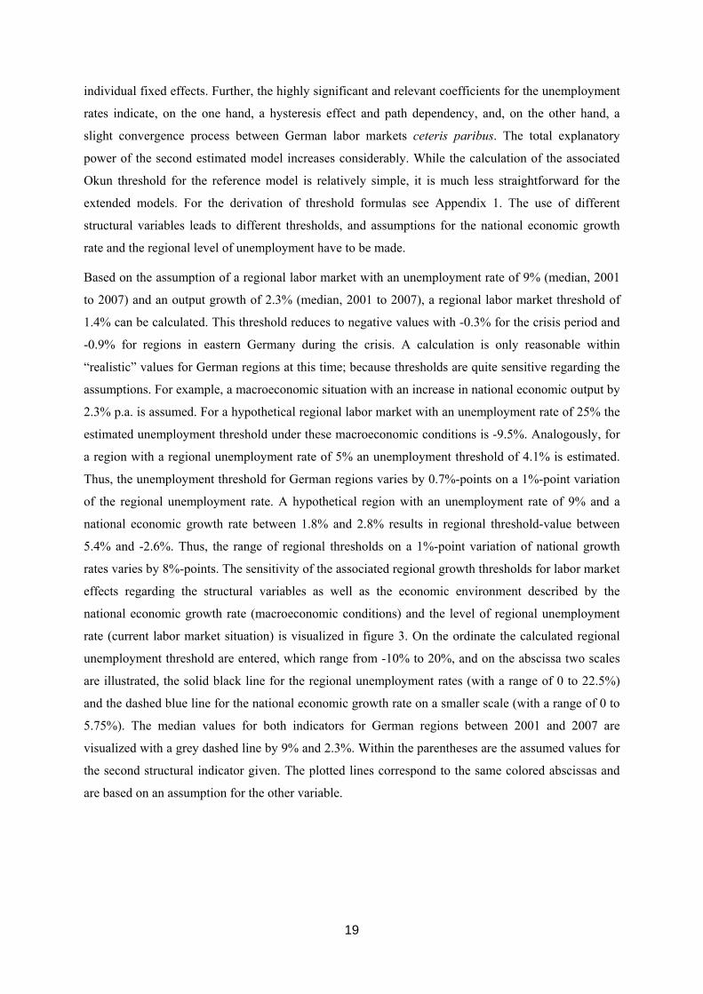
rates varies by 8%-points. The sensitivity of the associated regional growth thresholds for labor market
effects regarding the structural variables as well as the economic environment described by the
national economic growth rate (macroeconomic conditions) and the level of regional unemployment
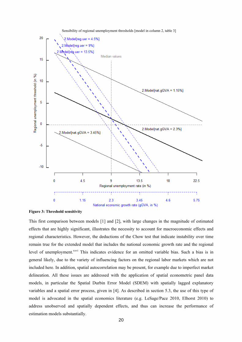
rate (current labor market situation) is visualized in figure 3. On the ordinate the calculated regional
unemployment threshold are entered, which range from -10% to 20%, and on the abscissa two scales
are illustrated, the solid black line for the regional unemployment rates (with a range of 0 to 22.5%)
and the dashed blue line for the national economic growth rate on a smaller scale (with a range of 0 to
5.75%). The median values for both indicators for German regions between 2001 and 2007 are
visualized with a grey dashed line by 9% and 2.3%. Within the parentheses are the assumed values for
the second structural indicator given. The plotted lines correspond to the same colored abscissas and
are based on an assumption for the other variable.
20
Figure 3: Threshold sensitivity
This first comparison between models [1] and [2], with large changes in the magnitude of estimated
effects that are highly significant, illustrates the necessity to account for macroeconomic effects and
regional characteristics. However, the deductions of the Chow test that indicate instability over time
remain true for the extended model that includes the national economic growth rate and the regional
level of unemployment.xxvi This indicates evidence for an omitted variable bias. Such a bias is in
general likely, due to the variety of influencing factors on the regional labor markets which are not
included here. In addition, spatial autocorrelation may be present, for example due to imperfect market
delineation. All these issues are addressed with the application of spatial econometric panel data
models, in particular the Spatial Durbin Error Model (SDEM) with spatially lagged explanatory
variables and a spatial error process, given in [4]. As described in section 5.3, the use of this type of
model is advocated in the spatial economics literature (e.g. LeSage/Pace 2010, Elhorst 2010) to
address unobserved and spatially dependent effects, and thus can increase the performance of
estimation models substantially.
Sensibility of regional unemployment thresholds [model in column 2, table 3]
21
A direct integration of the set of explanatory variables X and optional fixed effects into a SDEM
structure can result in multicollinearity problems, caused in particular by the structural dummy
variable east (x3) (see the overview on variance inflation factors provided in Appendix 3). Therefore,
the dummy variable east (x3) is dropped in the following analysis due to its insignificance in the
foregoing estimation and multicollinearity problems. In the 3rd column of table 3 the results are given
for a SDEM with the extended set of explanatory variables X based on equation [3]. The regional level
of unemployment rate is interacted with the dummy variable for the crisis (x6·x4) to control for
regional differences in response towards the crisis. The spatial lag of this interaction term is not
included, again due to multicollinearity problems. In the 4th, 5th and 6th column the results for the
estimations on the combined SDEM and regional individual fixed effects model are presented, see
equations [6], [7] and [8]. Those allow capturing the regional heterogeneous characteristics and/or
differences in regional response towards the economic crisis, while accounting simultaneously for
spatial dependency and non-systematic linkages between regional markets. The models in columns 4
and 6 include an individual intercept for each region, while in the 3rd and 5th column the substitute
variable level of unemployment rates (x6) is applied. To capture a regional heterogeneous response
towards the economic crisis, the models in columns 3 and 4 contain an interaction term between the
regional level of unemployment with the dummy variable for the crisis (x6·x4), while the models in
column 5 and 6 consist of vectors for the regional intercepts multiplied with the crisis dummy variable
(αR·x4). Note that for the model of column 5 the response towards the economic crisis in 2008 to 2009
takes into account an interaction term of regional characteristics with the crisis dummy variable
(x6·x4); and therefore the dummy variable for the crisis itself is dropped.
The estimation results for the SDEM confirm the rather low regional Okun coefficients of
around -0.05 in the dynamic perspective. From the newly added parameters in the SDEMs, the
spatially lagged regional economic growth rates of W·x1 ≈ -0.04 and the spatially and time-lagged
regional economic growth rates W·x2 ≈ -0.06 are indicated as significant. W·x1 is the effect of the
average growth in the neighboring regions on the regional labor market, and W·x2 the same for the
growth rates in the previous period. Although the primary motivation for including spatial lags is to
capture unobserved effects, the slightly higher magnitude may require some explanation. For those
spatial lags it must be considered that this is a cumulative effect over neighboring regions,
summarizing the effects over all regarded regions (Lerbs/Oberst, 2012). With the SDEM, the
explanatory power of the estimation increases once again. There is no general preference for the
SDEMs with fixed effects in the form of dummy variables (see e.g. 4th column in table 3) or the
SDEMs using the substitute variable. Both types of models basically tell the same story and, if
anything, this shows the robustness of the Okun estimators. However, the regional individual fixed
effects and their interaction term for the regional heterogeneous response towards the crisis are ideal to
map geographically, while for the alternative variables a general economic interpretation is more
obvious.
22
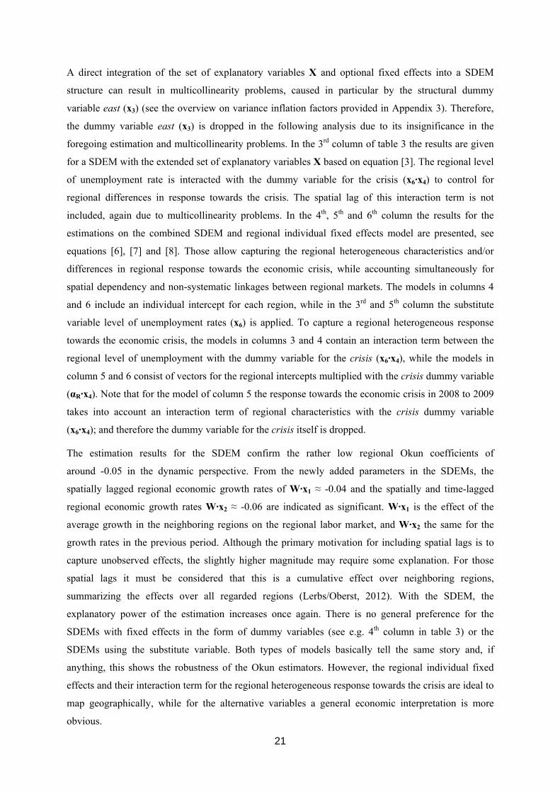
Figure 4: Growth effects on the regional labor market (model comparison)
For a model comparison of the estimated economic growth effects on the regional labor markets and
its separation into regional, national and neighbor-region growth effects see figure 4. This illustration
supports the conclusion of the robustness of the results. The resulting overall effect of about 0.5 is
comparable with estimates in macroeconomic analysis for Germany (see e.g. Schalk/Lüschow/Untiedt
(1997), Moosa (1997), OECD (2010)). The magnitude of the cumulative neighbor effect can primarily
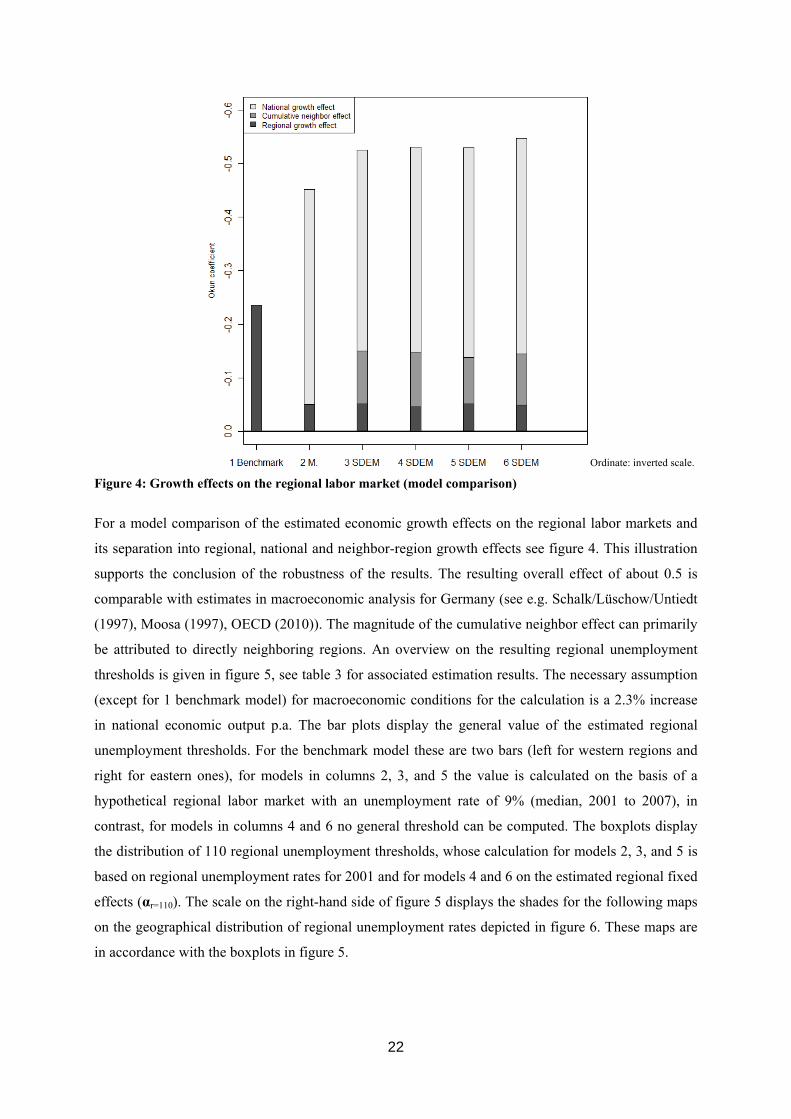
be attributed to directly neighboring regions. An overview on the resulting regional unemployment
thresholds is given in figure 5, see table 3 for associated estimation results. The necessary assumption
(except for 1 benchmark model) for macroeconomic conditions for the calculation is a 2.3% increase
in national economic output p.a. The bar plots display the general value of the estimated regional
unemployment thresholds. For the benchmark model these are two bars (left for western regions and
right for eastern ones), for models in columns 2, 3, and 5 the value is calculated on the basis of a
hypothetical regional labor market with an unemployment rate of 9% (median, 2001 to 2007), in
contrast, for models in columns 4 and 6 no general threshold can be computed. The boxplots display
the distribution of 110 regional unemployment thresholds, whose calculation for models 2, 3, and 5 is
based on regional unemployment rates for 2001 and for models 4 and 6 on the estimated regional fixed
effects (αr=110). The scale on the right-hand side of figure 5 displays the shades for the following maps
on the geographical distribution of regional unemployment rates depicted in figure 6. These maps are
in accordance with the boxplots in figure 5.
Ordinate: inverted scale.
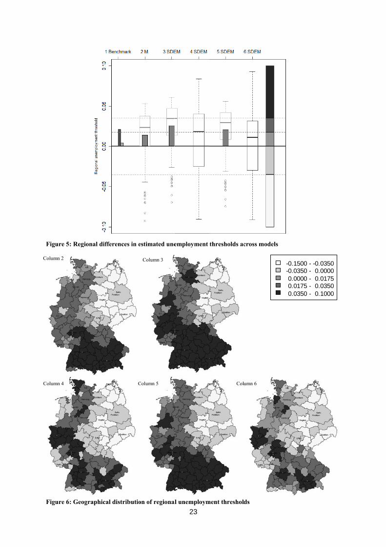
Figure 5
Figure 6
Column 2
Column 4
: Regional di
: Geographic
fferences in e
cal distributio
C
estimated une
on of regiona
Column 3
Column 5
23
employment
al unemploym
thresholds ac
ment threshold
Colu
cross models
ds
umn 6
-0.1500 - --0.0350 - 0.0000 - 0.0175 - 0.0350 -
-0.03500.00000.01750.03500.1000
24
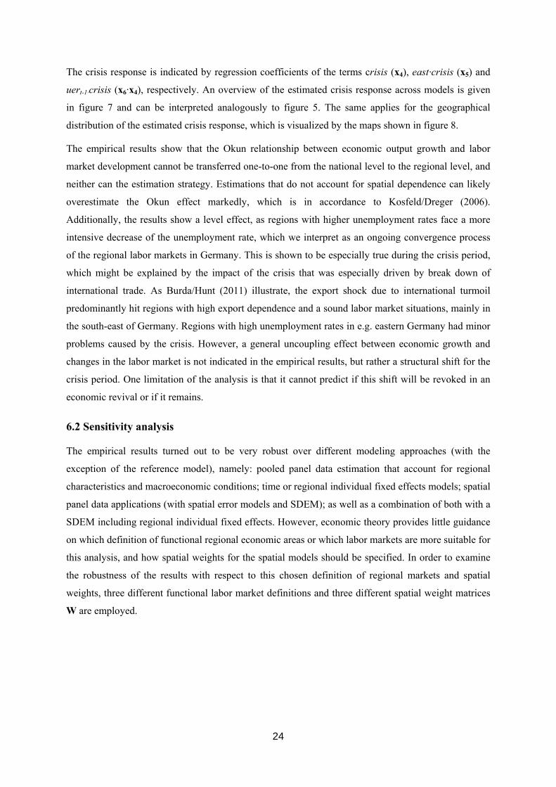
The crisis response is indicated by regression coefficients of the terms crisis (x4), east·crisis (x5) and
uert-1·crisis (x6·x4), respectively. An overview of the estimated crisis response across models is given
in figure 7 and can be interpreted analogously to figure 5. The same applies for the geographical
distribution of the estimated crisis response, which is visualized by the maps shown in figure 8.
The empirical results show that the Okun relationship between economic output growth and labor
market development cannot be transferred one-to-one from the national level to the regional level, and
neither can the estimation strategy. Estimations that do not account for spatial dependence can likely
overestimate the Okun effect markedly, which is in accordance to Kosfeld/Dreger (2006).
Additionally, the results show a level effect, as regions with higher unemployment rates face a more
intensive decrease of the unemployment rate, which we interpret as an ongoing convergence process
of the regional labor markets in Germany. This is shown to be especially true during the crisis period,
which might be explained by the impact of the crisis that was especially driven by break down of
international trade. As Burda/Hunt (2011) illustrate, the export shock due to international turmoil
predominantly hit regions with high export dependence and a sound labor market situations, mainly in
the south-east of Germany. Regions with high unemployment rates in e.g. eastern Germany had minor
problems caused by the crisis. However, a general uncoupling effect between economic growth and
changes in the labor market is not indicated in the empirical results, but rather a structural shift for the
crisis period. One limitation of the analysis is that it cannot predict if this shift will be revoked in an
economic revival or if it remains.
6.2 Sensitivity analysis
The empirical results turned out to be very robust over different modeling approaches (with the
exception of the reference model), namely: pooled panel data estimation that account for regional
characteristics and macroeconomic conditions; time or regional individual fixed effects models; spatial
panel data applications (with spatial error models and SDEM); as well as a combination of both with a
SDEM including regional individual fixed effects. However, economic theory provides little guidance
on which definition of functional regional economic areas or which labor markets are more suitable for
this analysis, and how spatial weights for the spatial models should be specified. In order to examine
the robustness of the results with respect to this chosen definition of regional markets and spatial
weights, three different functional labor market definitions and three different spatial weight matrices
W are employed.
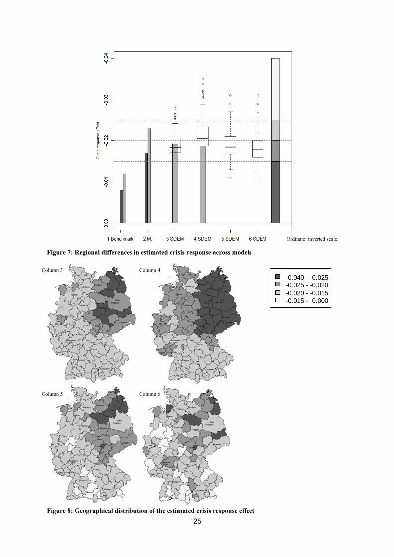
Figure 7
Figure 8
Column 3
Column 5
: Regional di
: Geographic
fferences in e
cal distributio
C
C
estimated cris
on of the estim
Column 4
Column 6
25
sis response a
mated crisis r
across model
response effe
s
ct
-0.040 - -0.0-0.025 - -0.0-0.020 - -0.0-0.015 - 0.0
Ordinate: invert
025020015000
ed scale.
26
The results for our 110 reference regions (Oberst, 2012) are compared with those for 50 labor market
regions defined by Kropp/Schwengler (2011), and the 413 adminstrative districts.xxvii The delineation
by Oberst (2012) is based on an evolutionary computational cluster analysis approach, while
Kropp/Schwengler (2011) use a graph theory approach. Both delineation procedures are applied on
commuting patterns and are aligned with the boundaries of the 413 administrative districts. On the one
hand, this selection covers a variety of delineation approaches and on the other hand a bandwidth of
different quantity and size of regions, whereby the reference regions here can be classified as middle
sized and more homogenous in structure. The results on the basis of the alternative 50 labor market
regions mainly confirm the previous presented ones. The utilization of the 413 administrative districts
illustrates the shortcomings of administrative borders for regional economic analysis and its distorting
effects on estimation results. In a second step, spatial weights matrixes W are varied. In addition to the
first-order queen contiguity matrix, all calculations are performed for a four nearest neighbor inverse-
distance matrix (using Euclidean distances between the regions centroids) and for a 90-km threshold-
distance matrix. The results turned out to be largely insensitive to the alternative weight matrices.xxviii
7 Conclusion and outlook
Our results confirm the assumption of a positive impact of economic growth on labor market
performance. Although it is likely that other impact factors apart from economic growth influence the
utilization ratio of the labor force as well, we conclude that economic growth is an important driving
force on regional labor market effects - or at least an appropriate summarizing indicator for these
regional economic developments. However, the estimated effect of regional economic growth for
German regions is far lower than it would have been expected in view of the macroeconomic literature
on Okun’s law. On the one hand, this might be attributable to the regional study areas rather than
national economies and, on the other hand, to the drawbacks of spatial dependency, to regional
characteristics and to omitted variable bias if regionalized Okun models are designed inappropriate, as
discussed in this paper. Our empirical finding for a regionalized Okun coefficient for German regions
is in a dynamic perspective about 0.05, meaning that a region with a 1% additional growth in regional
economic output undergoes a reduction of regional unemployment rate of 0.05 percentage points per
year (e.g. from 10% to 9.95%). About 0.03 percentage points occur directly in the same annual period
and 0.02 percentage points are time delayed until the following period. In comparison, an additional
national macroeconomic growth of 1% is estimated to correspond to a reduction of regional
unemployment rates by 0.4 percentage points per year (e.g. from 10% to 9.6%). This illustrates the
limited transferability of empirical results for the macroeconomic rule of thumb of Okun’s law for
growth dynamic to a disaggregated regional level, as well as the limitations of regional growth
dynamics for regional labor markets. Even when the analysis is based on functionally delineated
regions, effects and actions focused on a single regional market will, in addition to the macroeconomic
situation, be influenced by adjacent markets, and vice versa. This will occur on an even more intense

27
level if measures are limited to administrative borders and spillovers are neglected. These findings are
in line with Niebuhr (2003). The regional economic policy implication that can be derived for the
results presented here is an interesting albeit likely depressing one for regional growth strategies that
imply labor market effects with a regional focus.
As national economic growth rates are identified as a dominating influence on regional labor market
performance it becomes obvious, with regard to the heterogeneous structure of German labor markets,
that national prosperity does not reach all parts of the country equally in the long term. Thus, regional
characteristics such as sectoral structure, the level of infrastructure, urbanization, etc. and their
influence on labor-intensive growth should be areas for further research.xxix Here we conclude that
regional growth policies are not appropriate to regional and delimited labor market effects. Regarding
the suitability of Okun’s law in general, the identification of the national growth rate favors the
macroeconomic rule of thumb. However, it is also shown that regional characteristics and labor market
situations matter. Even though the growth patterns are shown to be significant and stable, the
heterogonous regional effects behind such a national indicator demonstrate its limitations.
On the methodological side, this paper shows that the drawbacks of omitted variable bias and spatial
dependency lead to overestimation of the relation between regional growth and changes in the labor
market. With all three extended estimation approaches, i.e. the fixed effects models, the spatial
models, and the combination of both, this overestimation in comparison to the benchmark model can
be identified. The ability of spatial models to capture unobserved effects can be shown by the
following contra-positioning: estimation results for the Okun relationship with the explanatory
variables from the reference model in a spatial model do match with the results from models that
control for macroeconomic conditions and regional characteristics. In a non-spatial setting the effects
without accounting for such factors are evidently overestimated. On the basis of the argument above
regarding the limited possibility of capturing all relevant impact factors on labor market developments
on a disaggregated regional level, the suitability and beneficial characteristics of the combined
approach of functional delineated labor markets and the Spatial Durbin Error Model (SDEM) is
elaborated theoretically and endorsed empirically in this paper.
28
Acknowledgments
The authors thank the participants of the 50th winter seminar of the GfR, the German speaking section
of the European Regional Science Association (Matrei/Ostirol, Austria), the Research Seminar in
Economics at the School of Business and Economics, RWTH Aachen University, and the CAWM
Doctoral Seminar at Muenster School of Business and Economics, University of Muenster. The
authors are also grateful to Reinhard Madlener and Ray Galvin for carefully editing this article. All
remaining errors are the authors’ responsibility.
References
Adanu, K. (2005): A cross-province comparison of Okun´s coefficient for Canada. Applied Economics, 37, 567-570.
Anselin, L.; Bera, A. (1998): Spatial Dependence in Linear Regression Models with an Introduction to Spatial Econometrics. In: Ullah A; Giles D. (eds.): Handbook of Applied Economic Statistics (New York: Marcel Dekker).
Anselin L.; Florax, R.; Rey, S.J. (eds.) (2004): Advances in spatial econometrics. Springer, Berlin.
Anselin, L.; Le Gallo, J.; Jayet, H. (2008): Spatial Panel Econometrics, In: Matyas, L.; Sevestre, P. (eds.), The Econometrics of Panel Data, Fundamentals and Recent Developments in Theory and Practice, 3rd Edition, Springer-Verlag, Berlin Heidelberg, 624-660.
Apergis, N.; Rezitis, A. (2003): An examination of Okun’s Law: evidence from regional areas in Greece. Applied Economics, 35, 1147-1151.
Ball, L.; Leigh, D.; Loungani, P. (2012): Okun’s Law: Fit at 50? IMF Conference Paper: http://www.imf.org/external/np/res/seminars/2012/arc/pdf/BLL.pdf
Baltagi, B. H., Song, S. H. Koh, W. (2007): Testing panel data regression models with spatial and serial error correlation. Journal of Econometrics, 140, 5-51.
Beaton, K. (2010): Time Variation in Okun’s Law: A Canada und U.S. Comparison. Bank of Canada, Working Paper, No. 2010-07.
Blanchard, O. (2004): Macroeconomics. 5th edition, Pearson, Upper Saddle River, New Jersey.
Burda, M. C.; Hunt, J. (2011): What explains the German labor market miracle in the great recession? NBER Working Paper No. 17187, http://www.nber.org/papers/w17187.
Carlino, G.; DeFina, R. (2006): Macroeconomic Analysis using regional data: an application to monetary policy. In: R. Arnott and D. McMillen (eds.), A Companion to Urban Economics, Oxford: Blackwell, 440-459.
Casado-Díaz, J. M. (2000): Local Labour Market Areas in Spain: A Case Study, Regional Studies, 34:9, 843-856.
Cazes, S.; Veric, S. (2011): What has happened to Okun’s Law in the US and Europe? Insights from the great recession and longer term trends. In: The Global Crisis: Causes, Responses and Challenges, Chapter 9, International Labour Office, Geneva.
29
Cazes, S.; Verick, S.; Al Huassami, F. (2011): Diverging trends in unemployment in the United States and Europe: Evidence from Okun’s Law and the global financial crisis. Employment Working Paper No. 106, International Labour Office, Geneva.
Chamberlin, G. (2011): Okun’s Law revisited. Office for National Statistics, Economic and Labour Market Review, February 2011.
Christopoulos, D. K. (2004): The relationship between output and unemployment: Evidence from Greek regions. Papers in Regional Science, 83, 611-620.
Cliff, A. D.; Ord, J. K. (1981): Spatial Processes: Models & Applications. Pion, London.
Daly, M.; Hobijn, B. (2010): Okun’s Law and the unemployment surprise of 2009. Federal Reserve Bank of San Francisco: FRBSF Economic Letter, 2010-07.
Dauth, W. (2010): Agglomeration and regional employment growth. IAB Discussion Paper, 7/2010.
Eckey, H.; Kosfeld, R.; Türck, M (2006): Abgrenzung deutscher Arbeitsmarktregionen. Raumordnung und Raumforschung, 64, 299-309.
Elhorst, J. P. (2003): The mystery of regional unemployment differentials: Theoretical and empirical explanations. Journal of Economic Surveys, 17(5), 709-748.
Elhorst, J.P. (2009): Spatial panel data models. In: Fischer, M. M.; Getis, A. (eds.): Handbook of Applied Spatial Analysis, Springer, Berlin.
Elhorst, J. P. (2010): Applied Spatial Econometrics: Raising the Bar. Spatial Economic Analysis, 5(1), 9-28.
Freeman, D. G. (2000): Regional Test of Okun’s Law. International advances in economic research, 6(3), 557-550.
Harris, R.; Silverstone, B. (2001): Testing for asymmetry in Okun’s law: A cross−country comparison. Economics Bulletin, 5(2), 1−13.
Herwartz, H.; Niebuhr, A. (2011): Growth, unemployment and labour institutions: evidence from a cross-section of EU regions. Applied Economics, 43, 4663-4676.
Hubert, F. (1997): Das Okun´sche Gesetz: Eine empirische Überprüfung für ausgewählte OECD-Länder unter besonderer Berücksichtigung der nationalen Arbeitsmarktordnungen. Arbeitspapier Nr. 13, Institut für Statistik und Ökonometrie, Johannes-Gutenberg Universität, Mainz.
IMF (2010): World Economic Outlook 2010. IMF, Washington D.C.
IMF (2012): World Economic Outlook (WEO) - Coping with High Debt and Sluggish Growth. IMF, Washington D.C.
Kangasharju, A.; Pehkonen, J. (2001): Employment-Output link in Finland: Evidence from regional data. Finnish Economic Papers, 14(1), 41-50.
Kangasharju, A.; Tavéra, C.; Nijkamp, P. (2011): Regional growth and unemployment. The validity of Okun’s law for the Finnish regions. Research Memorandum 2001-6: ftp://zappa.ubvu.vu.nl/20110006.pdf
30
Kholodilin, K. A.; Siliverstovs, B. (2012): Measuring Regional Inequality by Internet Car Price Advertisements: Evidence for Germany. Economics Letters, 116(3), 414-417.
Knotek, E. S. (2007): How Useful is Okun’s Law”. Economic Review, Federal Reserve Bank of Kansas City, 4, 73-103.
Kosfeld, R., Dreger, C. (2006): Thresholds for employment and unemployment: A spatial analysis of German regional labour markets, 1992-2000. Papers in Regional Science, 85(4), 523-542.
Kosfeld, R.; Werner, A. (2012): Deutsche Arbeitsmarktregionen – Neuabgrenzung nach den Kreisgebietsreformen 2007–2011. Raumforschung und Raumordnung, 70, 49-64.
Kropp, P.; Schwengler, B. (2011): Abgrenzung von Arbeitsmarktregionen – ein Methodenvorschlag. Raumordnung und Raumforschung 69, 45-62.
Krugman, P. (2009): Free to Lose. The New York Times, Op-Ed Page, November 12, http://www.nytimes.com/2009/11/13/opinion/13krugman.html
Lee, J. (2000): The Robustness of Okun’s Law: Evidence from OECD Countries. Journal of Macroeconomics, 22(2), 331-356.
Lerbs, O. W.; Oberst, C. A. (2012): Explaining the Spatial Variation in Homeownership Rates: Results for German Regions. Regional Studies, DOI:10.1080/00343404.2012.685464.
LeSage, J.; Pace, R. K. (2009): Introduction to Spatial Econometrics. Chapman & Hall/CRC, Boca Raton, Florida.
Malley, J.; Molana, H. (2008): Output, Unemployment and Okun’s Law: Some evidence from G7. Economic Letters, 101, 113-115.
McCombie, J. S. L.; de Ridder, J. R. (1984): “The Verdoorn Law controversy”: some new empirical evidence using U.S. State data. Oxford Economic Papers, 36, 268-284.
Michels, W.; Oberst, C.; Hiller, N. (2011): Wohnungsmarktregionen in Deutschland – Abgrenzung und Struktur funktionaler Wohnungsmärkte, Materialien zum Siedlungs- und Wohnungswesen 45, InSiWo, Münster. As well as online publication at: www.wuestenrot-stiftung.de/pdf/Wohnungsmarktregionen.pdf
Millo, G.; Piras, G. (2011): splm: Econometric Models for Spatial Panel Data. R package version 0.9-05/r131: http://r-forge.r-project.org/projects/splm/
Moazzami, B.; Dadgostar, B. (2009): Okun’s law Revisited: Evidence from OECD Countries. International Business & Economics Research Journal, 8(8), pp. 21-24.
Möller, J. (2010): The German labor market response in the world recession * de-mystifying a miracle. Zeitschrift für Arbeitsmarkt Forschung, 42(4), 325-336.
Moosa, I. A. (1997): A Cross-Country comparison of Okun´s coefficient. Journal of comparative Economics, 24, 335-356.
Nguyen, D. T.; Mahinda Siriwardana, A. (1988): The Relationship between Output Growth and Unemployment: A Re-examination of Okun's Law in Australia. Australian Economic Review 21(1), 16–27.
31
Niebuhr, A. (2003): Spatial Interaction and Regional Unemployment in Europe. European Journal of Spatial Development, 2003, No. 5.
Oberst, C. A. (2012) A Methodology Approach to Delineate Functional Economic Market Areas with an Iterative Three-Step Spatial Clustering Procedure. CAWM Discussion Paper No. 55.
OECD (2010): Employment Outlook 2010, OECD, Paris.
Okun, A. (1962): Potential GNP: Its Measurement and Significance, American Statistical Association, Proceedings of the Business and Economic Statistics Section: 98-104.
Owyang, M. T.; Sekhposyan, T. (2012): Okuns’s Law over the Business Cycle: Was the Great Recession all that differen? Federal Reserve Bank of St. Louis Review, 94(5), 399-418.
Palley, T. I. (1993): Okun's Law and the asymmetric and changing cyclical behaviour of the USA economy. International Review of Applied Economics, 7(2).
Perugini, C.; Signorelli, M. (2005): Growth and employment in EU countries and regions. Presented at: “XX “Convegno Nazionale degli Economisti del Lavoro” (AIEL), Rome, September 22-23. http://www.aiel.it/bacheca/ROMA/Free_contributions/Regioni/perugini_signorelli.pdf
Pierdzioch, C.; Rülke, J.-C.; Stadtmann, G. (2012): Is there a Core of Macroeconomics that Euro Area Forecasters Believe In? German Economic Review, 13(1), 103-115.
Royuela, V.; Vargas, M. (2007): Defining Housing Market Areas using Commuting and Migration Algorithms. Catalonia (Spain) as an applied case study. Urban Studies, 46(11), 2381-2398.
Schalk, H.-J., Lüschow, J.; Untiedt, G. (1997): Wachstum und Arbeitslosigkeit – Gibt es noch einen Zusammenhang? Ifo-Schnelldienst, 17-18/1997.
Schäfer, H. (2005): Beschäftigungs- und Arbeitslosigkeitsschwellen - Interpretation und internationaler Vergleich. IW-Trends – Vierteljahresschrift zur empirischen Wirtschaftsforschung, 32(2), 1-12.
Simpson, E. H. (1951): The interpretation of interaction in contingency tables. Journal of the Royal Statistical Society B, 13(2), 228-241.
Sögner, L.; Stiassny, A. (2002): An analysis on the structural stability of Okun’s Law – a cross-country study. Applied Economics, 2002 (14), 1775-1787.
Stock, L.; Vogler-Ludwig, K. (2010): NAIRU and Okun’s Law – The Macro-Economy in a Nutshell? Thematic paper for the European Employment Observatory of the European Commission, Directorate General for Employment, Social Affairs and Equal Opportunities, Brussels.
Villaverde, J.; Maza, A. (2009): The robustness of Okun’s law in Spain, 1980-2004 Regional evidence. Journal of Policy Modeling, 31, 289-297.
Yazgan, M. E.; Yilmazkuday, H. (2009): Okun’s convergence within the US. Letters in Spatial and Resource Sciences, 2, 109-122.
Zierahn, U. (2012): The importance of spatial autocorrelation for regional employment growth in Germany. Jahrbuch der Regionalwissenschaften, 32, 19-43.
32
Notes
i This expression is widely used in the literature concerning Okun’s law; see for example Harris/Silverstone (2001), Freeman (2000), Palley (1993), and Nguyen/Siriwardana (1988). ii The asymmetric development of the Okun coefficient in times of recession compared to expansions is shown by Harris/Silverstone (2001) and is confirmed for Canada and the USA by Beaton (2010). iii Lee (2000), for example, identifies different results for the first-difference and the gap approach. iv The gap version is in line with the original approach of Okun as the output gap is chosen as the parameter for the economic development and the natural unemployment rate for the labor market. Both the potential output and the natural unemployment rate have to be estimated. This is inappropriate for this study, as an estimation of both variables on regional level would lead to further problems and blurry results. v Apergis/Rezitis (2003) estimates quite similar Okun coefficients for six out of eight Greek regions and find, using a first-difference variation, a structural break in 1981. vi A critical review of the influence of sectoral structures on regional unemployment rates can be found in Elhorst (2003). vii In his critical review on Okun’s law, Knotek (2010) suggests to use dynamic aspects. viii Further alternative regional labor market definitions for Germany can be found in Eckey/Kosfeld/Türck (2006) and Kosfeld/Werner (2012). ix See Michels/Oberst/Hiller (2011). In addition, Royuela/Vargas (2007), using a delineation approach, find that housing markets defined on commuting areas are more homogenous in price than those defined on migration patterns. x The dependent variable of change in unemployment rates is available up to 2002. The main explanatory variable of economic growth, measured in GVA, is available until 2009. xi Apergis/Rezitis (2003) use a slightly different approach, as they split their regression into two estimations for the pre- and post-period of the structural break for Greek areas. The approach used here is in line with Schalk/Untied/Lüschow (1997). xii There are some concerns about using regional housing prices as an approximation for regional differences in the inflation rate, e.g. potential endogeneity problems with the dependent variable and the major explanatory variable of economic growth. The question whether it reflects asset-price inflation or if it reflects inflation on consumer goods has to be discussed. Nonetheless, this is an important area for future research and the authors are thankful to C C Michelsen for intense discussions about this issue.
xiii The growth of “all other regions” is calculated as follows: .11,
,
rkRktr
rkRktr
GVA
GVA
The total of absolute values for differences between national economic growth rates and the calculated growth of all other regions for the 880 observations is 0.1096, the standard deviation of these differences is 0.0003. The correlation between the national economic growth rates and the calculated growth of “all other regions” is 0.99993. xiv See Lerbs/Oberst (2012).
xv Moran’s I is defined as: ;)(
))((
1
2
1 1
0
N
ii
N
i
N
jjiij
xx
xxxxw
W
NI with
N
i
N
jijwW
1 10 .
33
xvi Another common type of systematic linkages between regions is migration flows, which, however, are strongly correlated with commuting patterns. xvii See a comparable argument in favor of a spatial error in Lerbs/Oberst (2012). xviii Besides the pooled and fixed effects model, there is a third type of panel model: the random effects model. The random effects model is less restricted than the fixed effects model, and its estimators of regression coefficients can be more statistically efficient, but its individual effects are assumed to be not correlated with the included explanatory variables. However, there is most likely to be such correlation in the employed regional panel data set, which can be confirmed with a formal statistical test (Hausman-test). xix Note that there are attempts to quantify regional inflation rates. See, for example, Kholodilin/Silverstovs (2012). However, the published regional inflation rates are on a different spatial reference level. xx LeSage/Pace (2010) point out that spatial dependence amplifies conventional omitted variable bias when there is non-zero correlation between the included explanatory variables and any omitted regional characteristics. The magnitude of bias amplification depends on the relative strength of spatial dependence in the dependent and the independent variables and the disturbances. Independence of included and unobserved variables in this regional panel is unlikely here, given that any latent regional characteristics, labor market developments and growth factors should exhibit very similar patterns of spatial dependence. xxi See a comparable statement in Lerbs/Oberst (2012). xxii See Millo/Piras (2011) according to Baltagi et. al. (2007), Anselin/LeGallo/Jayet (2008), Elhorst (2009), and others. xxiii The estimators are the same as if the model is estimated with ordinary least square (OLS); only the standard errors differ very slightly (with no consequences for the indicated significance). xxiv The thresholds indicate the economic growth required to keep the unemployment rate constant. xxv The hypothesis of stability over time can be rejected at common significance levels, while across regions it cannot. Both times a so-called Chow test is applied. Even though the hypothesis of parameter stability across regions cannot be formally rejected, it is doubtful that it has an effect on the relationship (as estimation results will confirm later on). Therefore, the effect of different characteristics on the regional labor markets is tested next, in addition to account for macroeconomic effects. The latter should ensure stability of the estimation over time. Adanu (2005) shows, for example, that the Okun coefficient depends on the regional degree of industrialization and the size of the population. Chow test statistics: the stability of the estimated relationship in [1] between regions cannot be rejected at the common significance level (F = 0.33, df1 = 108, df2 = 766, p-value = 1.00), but only the stability over time of the coefficients can be rejected F = 408.6, df1 = 6, df2 =868, p-value = 0.00). xxvi Test on stability over regions, F = 0.6327, df1= 109, df2= 763, p-value = 0.9984; on stability over time: F = 198.81, df1=5, df2=867, p-value = 0.00. xxvii For a comparison of six different labor market delineations see Kropp/Schwengler (2012). xxviii The results are available from the authors upon request. xxix There is still some research being done on this topic; see, among others, Dauth (2010), Elhorst (2003) or Zierahn (2012).
List of FCN Working Papers
2013 Grieser B., Madlener R., Sunak Y. (2013). Economics of Small Wind Power Plants in Urban Settings: An Empirical
Investigation for Germany, FCN Working Paper No. 1/2013, Institute for Future Energy Consumer Needs and Behavior, RWTH Aachen University, January.
Madlener R., Specht J.M. (2013). An Exploratory Economic Analysis of Underground Pumped-Storage Hydro
Power Plants in Abandoned Coal Mines, FCN Working Paper No. 2/2013, Institute for Future Energy Consumer Needs and Behavior, RWTH Aachen University, February.
Kroniger D., Madlener R. (2013). Hydrogen Storage for Wind Parks: A Real Options Evaluation for an Optimal
Investment in More Flexibility, FCN Working Paper No. 3/2013, Institute for Future Energy Consumer Needs and Behavior, RWTH Aachen University, February.
Petersen C., Madlener R. (2013). The Impact of Distributed Generation from Renewables on the Valuation and
Marketing of Coal-Fired and IGCC Power Plants, FCN Working Paper No. 4/2013, Institute for Future Energy Consumer Needs and Behavior, RWTH Aachen University, February.
Oberst C.A., Oelgemöller J. (2013). Economic Growth and Regional Labor Market Development in German
Regions: Okun’s Law in a Spatial Context, FCN Working Paper No. 5/2013, Institute for Future Energy Consumer Needs and Behavior, RWTH Aachen University, March.
2012 Ghosh G., Shortle J. (2012). Managing Pollution Risk through Emissions Trading, FCN Working Paper
No. 1/2012, Institute for Future Energy Consumer Needs and Behavior, RWTH Aachen University, January. Palzer A., Westner G., Madlener M. (2012). Evaluation of Different Hedging Strategies for Commodity Price Risks
of Industrial Cogeneration Plants, FCN Working Paper No. 2/2012, Institute for Future Energy Consumer Needs and Behavior, RWTH Aachen University, March (revised March 2013).
Sunak Y., Madlener R. (2012). The Impact of Wind Farms on Property Values: A Geographically Weighted
Hedonic Pricing Model, FCN Working Paper No. 3/2012, Institute for Future Energy Consumer Needs and Behavior, RWTH Aachen University, May (revised March 2013).
Achtnicht M., Madlener R. (2012). Factors Influencing German House Owners' Preferences on Energy Retrofits,
FCN Working Paper No. 4/2012, Institute for Future Energy Consumer Needs and Behavior, RWTH Aachen University, June.
Schabram J., Madlener R. (2012). The German Market Premium for Renewable Electricity: Profitability and Risk
of Self-Marketing, FCN Working Paper No. 5/2012, Institute for Future Energy Consumer Needs and Behavior, RWTH Aachen University, July.
Garbuzova M., Madlener R. (2012). Russia’s Emerging ESCO Market: Prospects and Barriers for Energy
Efficiency Investments, FCN Working Paper No. 6/2012, Institute for Future Energy Consumer Needs and Behavior, RWTH Aachen University, July (revised December 2012).
Rosen C., Madlener R. (2012). Auction Design for Local Reserve Energy Markets, FCN Working Paper No.
7/2012, Institute for Future Energy Consumer Needs and Behavior, RWTH Aachen University, July (revised March 2013).
Sorda G., Madlener R. (2012). Cost-Effectiveness of Lignocellulose Biorefineries and their Impact on the
Deciduous Wood Markets in Germany. FCN Working Paper No. 8/2012, Institute for Future Energy Consumer Needs and Behavior, RWTH Aachen University, September.
Madlener R., Ortlieb C. (2012). An Investigation of the Economic Viability of Wave Energy Technology: The Case of the Ocean Harvester, FCN Working Paper No. 9/2012, Institute for Future Energy Consumer Needs and Behavior, RWTH Aachen University, October.
Hampe J., Madlener R. (2012). Economics of High-Temperature Nuclear Reactors for Industrial Cogeneration,
FCN Working Paper No. 10/2012, Institute for Future Energy Consumer Needs and Behavior, RWTH Aachen University, October.
Knaut A., Madlener R., Rosen C., Vogt C. (2012). Impact of Temperature Uncertainty on the Economic Valuation
of Geothermal Projects: A Real Options Approach, FCN Working Paper No. 11/2012, Institute for Future Energy Consumer Needs and Behavior, RWTH Aachen University, November.
Hünteler J., Niebuhr C.F., Schmidt T.S., Madlener R., Hoffmann V.H. (2012). Financing Feed-in Tariffs in
Developing Countries under a Post-Kyoto Climate Policy Regime: A Case Study of Thailand, FCN Working Paper No. 12/2012, Institute for Future Energy Consumer Needs and Behavior, RWTH Aachen University, December.
Blass N., Madlener R. (2012). Structural Inefficiencies and Benchmarking of Water Supply Companies in
Germany, FCN Working Paper No. 13/2012, Institute for Future Energy Consumer Needs and Behavior, RWTH Aachen University, December.
Madlener R., Schabram J. (2012). Predicting Reserve Energy from New Renewables by Means of Principal
Component Analysis and Copula Functions, FCN Working Paper No. 14/2012, Institute for Future Energy Consumer Needs and Behavior, RWTH Aachen University, December.
Harzendorf F., Madlener R. (2012). Optimal Investment in Gas-Fired Engine-CHP Plants in Germany: A Real
Options Approach, FCN Working Paper No. 15/2012, Institute for Future Energy Consumer Needs and Behavior, RWTH Aachen University, December.
Schmitz M., Madlener R. (2012). Economic Feasibility of Kite-Based Wind Energy Powerships with CAES or
Hydrogen Storage, FCN Working Paper No. 16/2012, Institute for Future Energy Consumer Needs and Behavior, RWTH Aachen University, December.
Dergiades T., Christofidou G., Madlener R. (2012). The Nexus between Natural Gas Spot and Futures Prices at
NYMEX: What about Non-Linear Causality?, FCN Working Paper No. 17/2012, Institute for Future Energy Consumer Needs and Behavior, RWTH Aachen University, December.
Rohlfs W., Madlener R. (2012). Assessment of Clean-Coal Strategies: The Questionable Merits of Carbon
Capture-Readiness, FCN Working Paper No. 18/2012, Institute for Future Energy Consumer Needs and Behavior, RWTH Aachen University, December.
Wüstemeyer C., Bunn D., Madlener R. (2012). Bridging the Gap between Onshore and Offshore Innovations by
the European Wind Power Supply Industry: A Survey-based Analysis, FCN Working Paper No. 19/2012, Institute for Future Energy Consumer Needs and Behavior, RWTH Aachen University, December.
Fuhrmann J., Madlener R. (2012). Evaluation of Synergies in the Context of European Multi-Business Utilities,
FCN Working Paper No. 20/2012, Institute for Future Energy Consumer Needs and Behavior, RWTH Aachen University, December.
2011 Sorda G., Sunak Y., Madlener R. (2011). A Spatial MAS Simulation to Evaluate the Promotion of Electricity from
Agricultural Biogas Plants in Germany, FCN Working Paper No. 1/2011, Institute for Future Energy Consumer Needs and Behavior, RWTH Aachen University, January (revised October 2012).
Madlener R., Hauertmann M. (2011). Rebound Effects in German Residential Heating: Do Ownership and Income
Matter?, FCN Working Paper No. 2/2011, Institute for Future Energy Consumer Needs and Behavior, RWTH Aachen University, February.
Garbuzova M., Madlener R. (2011). Towards an Efficient and Low-Carbon Economy Post-2012: Opportunities and
Barriers for Foreign Companies in the Russian Market, FCN Working Paper No. 3/2011, Institute for Future Energy Consumer Needs and Behavior, RWTH Aachen University, February (revised July 2011).
Westner G., Madlener R. (2011). The Impact of Modified EU ETS Allocation Principles on the Economics of CHP-
Based District Heating Networks. FCN Working Paper No. 4/2011, Institute for Future Energy Consumer Needs and Behavior, RWTH Aachen University, February.
Madlener R., Ruschhaupt J. (2011). Modeling the Influence of Network Externalities and Quality on Market Shares of Plug-in Hybrid Vehicles, FCN Working Paper No. 5/2011, Institute for Future Energy Consumer Needs and Behavior, RWTH Aachen University, March.
Juckenack S., Madlener R. (2011). Optimal Time to Start Serial Production: The Case of the Direct Drive Wind
Turbine of Siemens Wind Power A/S, FCN Working Paper No. 6/2011, Institute for Future Energy Consumer Needs and Behavior, RWTH Aachen University, March.
Madlener R., Sicking S. (2011). Assessing the Economic Potential of Microdrilling in Geothermal Exploration, FCN
Working Paper No. 7/2011, Institute for Future Energy Consumer Needs and Behavior, RWTH Aachen University, April.
Bernstein R., Madlener R. (2011). Responsiveness of Residential Electricity Demand in OECD Countries: A Panel
Cointegration and Causality Analysis, FCN Working Paper No. 8/2011, Institute for Future Energy Consumer Needs and Behavior, RWTH Aachen University, April.
Michelsen C.C., Madlener R. (2011). Homeowners' Preferences for Adopting Residential Heating Systems: A
Discrete Choice Analysis for Germany, FCN Working Paper No. 9/2011, Institute for Future Energy Consumer Needs and Behavior, RWTH Aachen University, May (revised January 2012).
Madlener R., Glensk B., Weber V. (2011). Fuzzy Portfolio Optimization of Onshore Wind Power Plants. FCN
Working Paper No. 10/2011, Institute for Future Energy Consumer Needs and Behavior, RWTH Aachen University, May.
Glensk B., Madlener R. (2011). Portfolio Selection Methods and their Empirical Applicability to Real Assets in
Energy Markets. FCN Working Paper No. 11/2011, Institute for Future Energy Consumer Needs and Behavior, RWTH Aachen University, May.
Kraas B., Schroedter-Homscheidt M., Pulvermüller B., Madlener R. (2011). Economic Assessment of a
Concentrating Solar Power Forecasting System for Participation in the Spanish Electricity Market, FCN Working Paper No. 12/2011, Institute for Future Energy Consumer Needs and Behavior, RWTH Aachen University, May.
Stocker A., Großmann A., Madlener R., Wolter M.I., (2011). Sustainable Energy Development in Austria Until
2020: Insights from Applying the Integrated Model “e3.at”, FCN Working Paper No. 13/2011, Institute for Future Energy Consumer Needs and Behavior, RWTH Aachen University, July.
Kumbaroğlu G., Madlener R. (2011). Evaluation of Economically Optimal Retrofit Investment Options for Energy
Savings in Buildings. FCN Working Paper No. 14/2011, Institute for Future Energy Consumer Needs and Behavior, RWTH Aachen University, September.
Bernstein R., Madlener R. (2011). Residential Natural Gas Demand Elasticities in OECD Countries: An ARDL
Bounds Testing Approach, FCN Working Paper No. 15/2011, Institute for Future Energy Consumer Needs and Behavior, RWTH Aachen University, October.
Glensk B., Madlener R. (2011). Dynamic Portfolio Selection Methods for Power Generation Assets, FCN Working
Paper No. 16/2011, Institute for Future Energy Consumer Needs and Behavior, RWTH Aachen University, November.
Michelsen C.C., Madlener R. (2011). Homeowners' Motivation to Adopt a Residential Heating System: A Principal-
Component Analysis, FCN Working Paper No. 17/2011, Institute for Future Energy Consumer Needs and Behavior, RWTH Aachen University, November (revised January 2013).
Razlaf J., Madlener R. (2011). Performance Measurement of CCS Power Plants Using the Capital Asset Pricing
Model, FCN Working Paper No. 18/2011, Institute for Future Energy Consumer Needs and Behavior, RWTH Aachen University, November.
Himpler S., Madlener R. (2011). Repowering of Wind Turbines: Economics and Optimal Timing, FCN Working
Paper No. 19/2011, Institute for Future Energy Consumer Needs and Behavior, RWTH Aachen University, November.
Hackbarth A., Madlener R. (2011). Consumer Preferences for Alternative Fuel Vehicles: A Discrete Choice
Analysis, FCN Working Paper No. 20/2011, Institute for Future Energy Consumer Needs and Behavior, RWTH Aachen University, December (revised December 2012).
Heuser B., Madlener R. (2011). Geothermal Heat and Power Generation with Binary Plants: A Two-Factor Real
Options Analysis, FCN Working Paper No. 21/2011, Institute for Future Energy Consumer Needs and Behavior, RWTH Aachen University, December.

Rohlfs W., Madlener R. (2011). Multi-Commodity Real Options Analysis of Power Plant Investments: Discounting Endogenous Risk Structures, FCN Working Paper No. 22/2011, Institute for Future Energy Consumer Needs and Behavior, RWTH Aachen University, December (revised July 2012).
2010 Lang J., Madlener R. (2010). Relevance of Risk Capital and Margining for the Valuation of Power Plants: Cash
Requirements for Credit Risk Mitigation, FCN Working Paper No. 1/2010, Institute for Future Energy Consumer Needs and Behavior, RWTH Aachen University, February.
Michelsen C.C., Madlener R. (2010). Integrated Theoretical Framework for a Homeowner’s Decision in Favor of
an Innovative Residential Heating System, FCN Working Paper No. 2/2010, Institute for Future Energy Consumer Needs and Behavior, RWTH Aachen University, February.
Harmsen - van Hout M.J.W., Herings P.J.-J., Dellaert B.G.C. (2010). The Structure of Online Consumer
Communication Networks, FCN Working Paper No. 3/2010, Institute for Future Energy Consumer Needs and Behavior, RWTH Aachen University, March.
Madlener R., Neustadt I. (2010). Renewable Energy Policy in the Presence of Innovation: Does Government Pre-
Commitment Matter?, FCN Working Paper No. 4/2010, Institute for Future Energy Consumer Needs and Behavior, RWTH Aachen University, April (revised June 2010 and December 2011).
Harmsen - van Hout M.J.W., Dellaert B.G.C., Herings, P.J.-J. (2010). Behavioral Effects in Individual Decisions of
Network Formation: Complexity Reduces Payoff Orientation and Social Preferences, FCN Working Paper No. 5/2010, Institute for Future Energy Consumer Needs and Behavior, RWTH Aachen University, May.
Lohwasser R., Madlener R. (2010). Relating R&D and Investment Policies to CCS Market Diffusion Through Two-
Factor Learning, FCN Working Paper No. 6/2010, Institute for Future Energy Consumer Needs and Behavior, RWTH Aachen University, June.
Rohlfs W., Madlener R. (2010). Valuation of CCS-Ready Coal-Fired Power Plants: A Multi-Dimensional Real
Options Approach, FCN Working Paper No. 7/2010, Institute for Future Energy Consumer Needs and Behavior, RWTH Aachen University, July.
Rohlfs W., Madlener R. (2010). Cost Effectiveness of Carbon Capture-Ready Coal Power Plants with Delayed
Retrofit, FCN Working Paper No. 8/2010, Institute for Future Energy Consumer Needs and Behavior, RWTH Aachen University, August (revised December 2010).
Gampert M., Madlener R. (2010). Pan-European Management of Electricity Portfolios: Risks and Opportunities of
Contract Bundling, FCN Working Paper No. 9/2010, Institute for Future Energy Consumer Needs and Behavior, RWTH Aachen University, August.
Glensk B., Madlener R. (2010). Fuzzy Portfolio Optimization for Power Generation Assets, FCN Working Paper
No. 10/2010, Institute for Future Energy Consumer Needs and Behavior, RWTH Aachen University, August. Lang J., Madlener R. (2010). Portfolio Optimization for Power Plants: The Impact of Credit Risk Mitigation and
Margining, FCN Working Paper No. 11/2010, Institute for Future Energy Consumer Needs and Behavior, RWTH Aachen University, September.
Westner G., Madlener R. (2010). Investment in New Power Generation Under Uncertainty: Benefits of CHP vs.
Condensing Plants in a Copula-Based Analysis, FCN Working Paper No. 12/2010, Institute for Future Energy Consumer Needs and Behavior, RWTH Aachen University, September.
Bellmann E., Lang J., Madlener R. (2010). Cost Evaluation of Credit Risk Securitization in the Electricity Industry:
Credit Default Acceptance vs. Margining Costs, FCN Working Paper No. 13/2010, Institute for Future Energy Consumer Needs and Behavior, RWTH Aachen University, September (revised May 2011).
Ernst C.-S., Lunz B., Hackbarth A., Madlener R., Sauer D.-U., Eckstein L. (2010). Optimal Battery Size for Serial
Plug-in Hybrid Vehicles: A Model-Based Economic Analysis for Germany, FCN Working Paper No. 14/2010, Institute for Future Energy Consumer Needs and Behavior, RWTH Aachen University, October (revised June 2011).
Harmsen - van Hout M.J.W., Herings P.J.-J., Dellaert B.G.C. (2010). Communication Network Formation with Link
Specificity and Value Transferability, FCN Working Paper No. 15/2010, Institute for Future Energy Consumer Needs and Behavior, RWTH Aachen University, November.
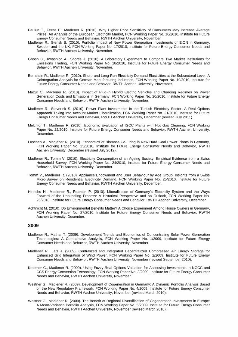
Paulun T., Feess E., Madlener R. (2010). Why Higher Price Sensitivity of Consumers May Increase Average Prices: An Analysis of the European Electricity Market, FCN Working Paper No. 16/2010, Institute for Future Energy Consumer Needs and Behavior, RWTH Aachen University, November.
Madlener R., Glensk B. (2010). Portfolio Impact of New Power Generation Investments of E.ON in Germany, Sweden and the UK, FCN Working Paper No. 17/2010, Institute for Future Energy Consumer Needs and Behavior, RWTH Aachen University, November.
Ghosh G., Kwasnica A., Shortle J. (2010). A Laboratory Experiment to Compare Two Market Institutions for
Emissions Trading, FCN Working Paper No. 18/2010, Institute for Future Energy Consumer Needs and Behavior, RWTH Aachen University, November.
Bernstein R., Madlener R. (2010). Short- and Long-Run Electricity Demand Elasticities at the Subsectoral Level: A
Cointegration Analysis for German Manufacturing Industries, FCN Working Paper No. 19/2010, Institute for Future Energy Consumer Needs and Behavior, RWTH Aachen University, November.
Mazur C., Madlener R. (2010). Impact of Plug-in Hybrid Electric Vehicles and Charging Regimes on Power
Generation Costs and Emissions in Germany, FCN Working Paper No. 20/2010, Institute for Future Energy Consumer Needs and Behavior, RWTH Aachen University, November.
Madlener R., Stoverink S. (2010). Power Plant Investments in the Turkish Electricity Sector: A Real Options
Approach Taking into Account Market Liberalization, FCN Working Paper No. 21/2010, Institute for Future Energy Consumer Needs and Behavior, RWTH Aachen University, December (revised July 2011).
Melchior T., Madlener R. (2010). Economic Evaluation of IGCC Plants with Hot Gas Cleaning, FCN Working
Paper No. 22/2010, Institute for Future Energy Consumer Needs and Behavior, RWTH Aachen University, December.
Lüschen A., Madlener R. (2010). Economics of Biomass Co-Firing in New Hard Coal Power Plants in Germany,
FCN Working Paper No. 23/2010, Institute for Future Energy Consumer Needs and Behavior, RWTH Aachen University, December (revised July 2012).
Madlener R., Tomm V. (2010). Electricity Consumption of an Ageing Society: Empirical Evidence from a Swiss
Household Survey, FCN Working Paper No. 24/2010, Institute for Future Energy Consumer Needs and Behavior, RWTH Aachen University, December.
Tomm V., Madlener R. (2010). Appliance Endowment and User Behaviour by Age Group: Insights from a Swiss
Micro-Survey on Residential Electricity Demand, FCN Working Paper No. 25/2010, Institute for Future Energy Consumer Needs and Behavior, RWTH Aachen University, December.
Hinrichs H., Madlener R., Pearson P. (2010). Liberalisation of Germany’s Electricity System and the Ways
Forward of the Unbundling Process: A Historical Perspective and an Outlook, FCN Working Paper No. 26/2010, Institute for Future Energy Consumer Needs and Behavior, RWTH Aachen University, December.
Achtnicht M. (2010). Do Environmental Benefits Matter? A Choice Experiment Among House Owners in Germany,
FCN Working Paper No. 27/2010, Institute for Future Energy Consumer Needs and Behavior, RWTH Aachen University, December.
2009 Madlener R., Mathar T. (2009). Development Trends and Economics of Concentrating Solar Power Generation
Technologies: A Comparative Analysis, FCN Working Paper No. 1/2009, Institute for Future Energy Consumer Needs and Behavior, RWTH Aachen University, November.
Madlener R., Latz J. (2009). Centralized and Integrated Decentralized Compressed Air Energy Storage for
Enhanced Grid Integration of Wind Power, FCN Working Paper No. 2/2009, Institute for Future Energy Consumer Needs and Behavior, RWTH Aachen University, November (revised September 2010).
Kraemer C., Madlener R. (2009). Using Fuzzy Real Options Valuation for Assessing Investments in NGCC and
CCS Energy Conversion Technology, FCN Working Paper No. 3/2009, Institute for Future Energy Consumer Needs and Behavior, RWTH Aachen University, November.
Westner G., Madlener R. (2009). Development of Cogeneration in Germany: A Dynamic Portfolio Analysis Based
on the New Regulatory Framework, FCN Working Paper No. 4/2009, Institute for Future Energy Consumer Needs and Behavior, RWTH Aachen University, November (revised March 2010).
Westner G., Madlener R. (2009). The Benefit of Regional Diversification of Cogeneration Investments in Europe:
A Mean-Variance Portfolio Analysis, FCN Working Paper No. 5/2009, Institute for Future Energy Consumer Needs and Behavior, RWTH Aachen University, November (revised March 2010).
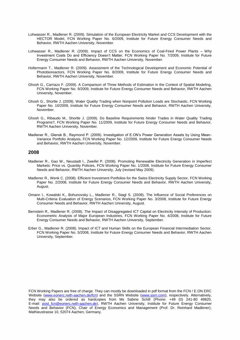
Lohwasser R., Madlener R. (2009). Simulation of the European Electricity Market and CCS Development with the
HECTOR Model, FCN Working Paper No. 6/2009, Institute for Future Energy Consumer Needs and Behavior, RWTH Aachen University, November.
Lohwasser R., Madlener R. (2009). Impact of CCS on the Economics of Coal-Fired Power Plants – Why
Investment Costs Do and Efficiency Doesn’t Matter, FCN Working Paper No. 7/2009, Institute for Future Energy Consumer Needs and Behavior, RWTH Aachen University, November.
Holtermann T., Madlener R. (2009). Assessment of the Technological Development and Economic Potential of
Photobioreactors, FCN Working Paper No. 8/2009, Institute for Future Energy Consumer Needs and Behavior, RWTH Aachen University, November.
Ghosh G., Carriazo F. (2009). A Comparison of Three Methods of Estimation in the Context of Spatial Modeling,
FCN Working Paper No. 9/2009, Institute for Future Energy Consumer Needs and Behavior, RWTH Aachen University, November.
Ghosh G., Shortle J. (2009). Water Quality Trading when Nonpoint Pollution Loads are Stochastic, FCN Working
Paper No. 10/2009, Institute for Future Energy Consumer Needs and Behavior, RWTH Aachen University, November.
Ghosh G., Ribaudo M., Shortle J. (2009). Do Baseline Requirements hinder Trades in Water Quality Trading
Programs?, FCN Working Paper No. 11/2009, Institute for Future Energy Consumer Needs and Behavior, RWTH Aachen University, November.
Madlener R., Glensk B., Raymond P. (2009). Investigation of E.ON’s Power Generation Assets by Using Mean-
Variance Portfolio Analysis, FCN Working Paper No. 12/2009, Institute for Future Energy Consumer Needs and Behavior, RWTH Aachen University, November.
2008 Madlener R., Gao W., Neustadt I., Zweifel P. (2008). Promoting Renewable Electricity Generation in Imperfect
Markets: Price vs. Quantity Policies, FCN Working Paper No. 1/2008, Institute for Future Energy Consumer Needs and Behavior, RWTH Aachen University, July (revised May 2009).
Madlener R., Wenk C. (2008). Efficient Investment Portfolios for the Swiss Electricity Supply Sector, FCN Working
Paper No. 2/2008, Institute for Future Energy Consumer Needs and Behavior, RWTH Aachen University, August.
Omann I., Kowalski K., Bohunovsky L., Madlener R., Stagl S. (2008). The Influence of Social Preferences on
Multi-Criteria Evaluation of Energy Scenarios, FCN Working Paper No. 3/2008, Institute for Future Energy Consumer Needs and Behavior, RWTH Aachen University, August.
Bernstein R., Madlener R. (2008). The Impact of Disaggregated ICT Capital on Electricity Intensity of Production:
Econometric Analysis of Major European Industries, FCN Working Paper No. 4/2008, Institute for Future Energy Consumer Needs and Behavior, RWTH Aachen University, September.
Erber G., Madlener R. (2008). Impact of ICT and Human Skills on the European Financial Intermediation Sector,
FCN Working Paper No. 5/2008, Institute for Future Energy Consumer Needs and Behavior, RWTH Aachen University, September.
FCN Working Papers are free of charge. They can mostly be downloaded in pdf format from the FCN / E.ON ERC Website (www.eonerc.rwth-aachen.de/fcn) and the SSRN Website (www.ssrn.com), respectively. Alternatively, they may also be ordered as hardcopies from Ms Sabine Schill (Phone: +49 (0) 241-80 49820, E-mail: [email protected]), RWTH Aachen University, Institute for Future Energy Consumer Needs and Behavior (FCN), Chair of Energy Economics and Management (Prof. Dr. Reinhard Madlener), Mathieustrasse 10, 52074 Aachen, Germany.