economic agents as imperfect problem solvers
TRANSCRIPT

Economic agents as imperfect problem solvers∗
Cosmin Ilut
Duke University & NBER
Rosen Valchev
Boston College
November 2017
Abstract
We develop a tractable model of limited cognitive perception of the optimal policy
function. Agents allocate cognitively costly reasoning effort to generate signals about the
optimal action conditional on the observed objective state. Accumulated signals update
beliefs about the entire function, but mostly about the optimal action conditional on
states close to the realizations where reasoning occurred. Agents reason more when
observing unusual states, producing state- and history-dependent responses akin to
salient thinking. The typical individual and aggregate actions exhibit non-linearity,
endogenous persistence and volatility clustering. Individual behavior also displays
stochastic choice, biases in systematic behavior, and cross-sectional volatility clusters.
Keywords: cognitively costly reasoning, imperfect perception of policy functions,
non-linearity, inertia and salience, endogenous persistence, time-varying volatility.
JEL Codes: D91, E32, E71.
∗Email addresses: Ilut [email protected], Valchev [email protected]. We would like to thank RyanChahrour, Tarek Hassan, Kristoffer Nimark, Philipp Sadowski, Todd Sarver and Mirko Wiederholt, as well asconference participants at the Green Line Macro Meetings, Society of Economic Dynamics and Computing inEconomics and Finance for helpful discussions and comments.
1 Introduction
Contrary to standard models where rational agents act optimally, in both real world and
experimental settings, economic agents often choose what appear to be sub-optimal actions,
especially when faced with complex situations. To account for that, the literature has become
increasingly interested in modeling cognitive limitations that constrain the agents’ ability
to reach the full information rational decision. This interest has come from different fields
including decision theory, behavioral economics, macroeconomics, finance and neuroscience
and has led to a diverse set of approaches. The common principle of these approaches is that
agents have limited cognitive resources to process payoff relevant information, and thus face
a trade-off in the accuracy of their eventual decision and the cognitive cost of reaching it.
A key modeling choice is the nature of the costly payoff-relevant information that agents
can choose to acquire. In general, a decision can be represented as a mapping from the
information about the objective states of the world to the set of considered actions. Therefore,
cognitive limitations in reaching the optimal decision may be relevant to two different layers
of imperfect perception. First, cognitive limitations may imply imperfect observation of the
objective states, such as income or interest rates. Second, cognitive limitations may imply
limited perception of the optimal mapping from information about the objective states to
the actual optimal action, such as consumption or labor.
The standard approach in the macroeconomics literature is to focus on the first layer
of uncertainty and assume that agents perceive the objective states with noise, but use
the mapping of information about the states to actions derived under full rationality. This
approach is exemplified by the Rational Inattention literature inspired by Sims (1998, 2003).1
More generally, the idea of allowing agents to choose their information about the unknown
objective states, but knowing what to do with it, is present in other parts of the literature.2
In this paper, we develop a tractable framework that focuses on the second layer
of imperfect perception. In our model agents observe all relevant objective state variables
perfectly. However, agents have limited cognitive resources that prevent them from computing
their optimal policy function and coming up with the optimal state-contingent plan of action.3
1Macroeconomic applications include consumption dynamics (Luo (2008), Tutino (2013)), price setting(Mackowiak and Wiederholt (2009), Stevens (2014), Matejka (2015)), monetary policy (Woodford (2009),Paciello and Wiederholt (2013)), business cycle dynamics (Melosi (2014), Mackowiak and Wiederholt (2015a))and portfolio choice (van Nieuwerburgh and Veldkamp (2009, 2010), Kacperczyk et al. (2016), Valchev (2017)).See Wiederholt (2010) and Sims (2010) for recent surveys on rational inattention in macroeconomics.
2See for example Woodford (2003), Reis (2006a,b) and Gabaix (2014, 2016). See Veldkamp (2011) for areview on imperfect information in macroeconomics and finance.
3Such a friction is consistent with a large field and laboratory experimental literature on how the qualityof decision making is negatively affected by the complexity of the decision problem. See Deck and Jahedi(2015) for a recent survey.
1

They can expend costly reasoning effort that helps reduce the uncertainty over the unknown
best course of action, and do so optimally.4 Given their chosen reasoning effort, agents
receive signals about the optimal action at the current state of the world, and the resulting
information about the optimal policy function accumulates over time. Thus, while being
imperfect problem solvers, agents are ‘procedurally rational’ in the sense of Simon (1976)
and exhibit behavior that is the outcome of appropriate deliberation.
In particular, the agent faces a tracking problem in the form of minimizing expected
squared deviations from the unknown optimal action. Therefore, the agent’s actual action is
the best guess, i.e. the expected value conditional on the accumulated information, of the
optimal policy function evaluated at the observed objective state. We model the uncertainty
about the unknown optimal policy function as a Gaussian Process distribution over which
agents update beliefs.5 A more intense reasoning effort is beneficial because it lowers the
variance of the noise in the incoming signals. In turn, a more intense reasoning is costly,
which we model as a cost on the total amount of information about the optimal action carried
in the new signal, as measured by the Shannon mutual information.6
The defining feature of our learning framework is the accumulation of information
about the optimal action as a function of the underlying state. The prior Gaussian Process
distribution is characterized by a stationary covariance function that controls the correlation
of beliefs about the values of the unknown function at distinct values of the objective state.
In particular, the information acquired about the value of the optimal action at some state
realization is perceived to be, at least partially, informative about the optimal action at
a different state realization. These knowledge spillovers across objective states lead to
propagation of the reasoning signals. When this correlation is imperfect, the information
acquired about the function is most useful locally to the state realization where reasoning
occurs. As a result, the uncertainty over the unknown policy function is lower around states
where reasoning has occurred more often.
The emerging key property of the decision to reason is intuitive: the agent finds it
optimal to reason more intensely when observing more unusual state realizations. These are
states where, given the reasoning history entering that period, the agent has a higher prior
4Generally, reasoning processes are characterized in the literature as ‘fact-free’ learning (see Aragoneset al. (2005)), i.e. because of cognitive limitations additional deliberation helps the agent get closer to theoptimal decision even without additional objective information as observed by an econometrician.
5Intuitively, a Gaussian Process distribution models a function as a vector of infinite length, where thevector has a joint Gaussian distribution. In addition to its wide-spread use in Bayesian statistics, GaussianProcesses have also been applied in machine learning over unknown functional relationships – both in termsof supervised (Rasmussen and Williams (2006)) and non-supervised (Bishop (2006)) learning.
6Following Sims (2003) a large literature has studied the choice properties of attention costs based on theShannon mutual information between prior and posterior beliefs. See for example Matejka and McKay (2014)Caplin et al. (2016), Woodford (2014) and Matejka et al. (2017).
2

uncertainty over the best course of action, conditional on the observed state. In contrast, at
states where past deliberation has occurred most often, the agent has accumulated sufficient
information so that further deliberation is not optimal. Thus, the deliberation choice and
actions are both state and history dependent, and display salient thinking. To characterize
the typical behavior, we focus on analyzing implications at the ergodic distribution, where
the agent has seen a long history of reasoning signals. To obtain a stable ergodic distribution
of beliefs, we also assume that the agent discounts past information at a constant rate.
The resulting behavior has several key properties. First, the ergodic policy function, i.e.
the action taken as a function of the observed state, is non-linear, even though the unknown
underlying optimal policy function is linear. This is due to the state dependent deliberation
choice. In particular, the ergodic prior uncertainty entering the period is U-shaped, being
smaller around the mean value of the objective state, where most of previous reasoning has
occurred. Therefore, for realizations in the middle of the state distribution, the agent chooses
not to reason much further and there the action is primarily driven by the prior knowledge
entering the period. In contrast, at realizations further in the tails of the state distribution, the
agent chooses to reason more intensely, and puts a larger weight on the new reasoning signal.
Thus, in this part of the state space the beliefs (and effective action) become increasingly
closer to the true unknown optimal action. Because of the resulting state-dependent weight
put on the new signal, the effective policy function becomes non-linear.
In our benchmark setup, which uses a non-informative, constant prior mean function,
the non-linearity manifests as an ergodic policy function that is relatively flat for state
realizations close to their mean (inertia), and much more responsive for tail realizations
(salience).7 Intuitively, the agent has a good understanding of the average level of the optimal
action around the mean of the state, and hence there is not much incentive to reason about
how the optimal policy changes with small movements in the state. The resulting imprecise
understanding of the shape of the optimal policy function leads towards a flat response around
usual states. In contrast, for state realizations further in the tail of the distribution, the
stronger incentive to reason leads to informative signals about the shape of the unknown
policy function, which on average point towards a more responsive action.
Second, there is endogenous persistence in both individual and aggregate actions.
This mechanism naturally arises from the knowledge spillovers acquired through reasoning.
Moreover, the interplay between the flat responses around the usual states and the salience
effects at the more unusual states generate local convexities in the ergodic policy function.
7The inertia is consistent with a widely documented ‘status-quo’ bias (Samuelson and Zeckhauser (1988)).The stronger response at unusual states is consistent with the so-called salience bias, or availability heuristic(Tversky and Kahneman (1975)), that makes behavior more sensitive to vivid, salient events.
3

The average movement in the periods following a change in the objective state may be
dominated by salience type of reasoning so that, even with mean reverting exogenous states,
the agent takes a more reactive action than before, leading to hump-shaped dynamics.
Third, there is endogenous time-variation in the volatility of actions. In samples that
happen to have more volatile state realizations the agent not only takes more volatile actions
but also chooses to reason more intensely. These stronger and more frequent incentives for
deliberation result in a posterior belief that the optimal action is more responsive. Therefore,
in periods following such volatile times, the actions appear to respond more to the objective
state, leading to clusters of volatility in actions, even without changes to structural parameters.
Agents also exhibit stochastic choice, an important behavior characteristic observed in
experiments. In our model, an agent’s action could vary even conditioning on the observed
state, due to the idiosyncratic reasoning signals and the fact that the optimal deliberation
choice depends on the whole history of objective states. At the same time, agents observe
different histories of reasoning signals leading to heterogeneous priors and policy functions.
This appears to an outside analyst as persistent biases in systematic behavior across agents.
We study cross-sectional effects by introducing a continuum of ex-ante identical agents
who solve the same reasoning problem and observe the same aggregate objective state.
However, the agents differ in their specific history of reasoning signals. At the more unusual
state realizations, where they have accumulated less relevant information, the agents’ priors
are more anchored by their common initial prior and the dispersion of beliefs entering the
period tends to be smaller. At the same time, at these states agents decide to rely more on
their newly obtained idiosyncratic reasoning signals. When the latter effect dominates, the
cross-sectional dispersion of actions is larger at the more unusual states.8
Finally, we extend our analysis to two actions that differ in their cost of making errors.
Since the information flow friction in our model is not over the single state variable, but is
specific to the cognitive effort it takes to make decisions about each action, the errors in the
two actions are not perfectly correlated. Moreover, the resulting effective policy functions are
different, even if the true unknown policy functions are the same. This contrasts with models
of imperfect perception of the objective state, where the mistakes in the two actions tend to
be perfectly correlated, as they are driven by the same belief over the unknown state.
Overall, we find that costly cognition can act as a parsimonious friction that generates
several important characteristics of many aggregate time-series: endogenous persistence,
non-linearity and volatility clustering, as well as possible hump-shaped dynamics. Therefore,
our findings connect three important directions in macroeconomics. One is a large literature
8Potential correlated volatility at the ’micro’ (cross-sectional dispersion) and ’macro’ (volatility clusteringof the aggregate action) level is consistent with recent evidence surveyed in Bloom (2014).
4

that proposes a set of frictions, typically taking the form of adjustment costs, to explain
sluggish behavior (eg. investment adjustment cost, habit formation in consumption, rigidities
in changing prices or wages).9 A second direction is to introduce frictions aimed at obtaining
non-linear dynamics (eg. search and matching labor models, financial constraints).10 Third,
there is a significant literature that documents and models exogenous variation in volatility
and structural parameters to better fit macroeconomic data.11
Relative to the literature on imperfect actions, the key property of our model is in
the dynamics of the distribution of beliefs over optimal actions. Compared to the standard
approach in macroeconomics, which analyzes imperfect perception of objective states, the
deliberation choice and the posterior uncertainty in our model are conditional on such states.12
Our emphasis on reasoning about optimal policy functions builds on a literature, mostly
in decision theory, that analyzes the costly perception of unknown subjective states.13 We
contribute to both of these strands of literature by developing a tractable model of learning
about the optimal action as an unknown function of the objective state. We characterize
how this form of learning leads to endogenous state and history dependence in the beliefs
entering the period. The resulting beliefs are instrumental to producing non-linear action
responses. Indeed, when we shut down the accumulation of information about the optimal
decision rule, we recover linear actions and uniform under-reaction to the state, a typical
result in the existing LQ Gaussian analysis of imperfect attention to objective states.14
Our costly cognition model also relates to two literatures on bounded rationality
in macroeconomics. One is a ‘near-rational’ approach that assumes a constant cost of
implementing the otherwise known optimal action. This work studies the general equilibrium
9See for example Christiano et al. (2005) and Smets and Wouters (2007).10See Fernandez-Villaverde et al. (2016) for a recent survey of non-linear methods.11For example Stock and Watson (2002), Cogley and Sargent (2005) and Justiniano and Primiceri (2008).12In that work the choice of attention to a state realization is typically made ex-ante, conditional on a
prior distribution over those realizations. Some recent models of ex-post attention choices, i.e conditional onthe current realization, include: the sparse operator of Gabaix (2014, 2016) that can be applied ex-ante orex-post to observing the state, information processing about the optimal action after a rare regime realizes(Mackowiak and Wiederholt (2015b)) and a decision over which information provider to use (Nimark andPitschner (2017)). The latter model can generate stronger agents’ responses to more extreme events becausethese events are more likely to be widely reported and be closer to common knowledge. Nimark (2014)obtains these stronger responses as a result of an assumed information structure where signals are more likelyto be available about more unusual events.
13As in the model of costly contemplation over tastes in Ergin and Sarver (2010) or the rationally inattentiveaxiomatization in Oliveira et al. (2017). Alaoui and Penta (2016) analyze a reasoning model where acquiringinformation about subjective mental states indexing payoffs is costly, but leads to higher accuracy.
14While there is interest in departures from that result, most of the focus in the literature has beenon obtaining optimal information structures that are non-Gaussian, taking the form of a discrete supportfor signals (see for example Sims (2006), Stevens (2014) and Matejka (2015)). Instead, we maintain thetractability of the LQ Gaussian setup but obtain non-linear dynamics.
5
(GE) effects of the resulting individual errors, taken as state-independent stochastic forces.15
A second literature addresses the potential difficulties faced by boundedly rational agents in
computing GE effects.16 There the individual decision rule is the same as the fully rational
one, but the GE effects are typically altered. Relative to these two approaches, we share an
interest in cognitive costs and focus on how imperfect reasoning generates an endogenous
structure of errors in actions, but abstract from GE effects for our aggregate implications.
The paper is organized as follows. Section 2 develops the cognitively costly reasoning
model. In Section 3 characterizes the ergodic distribution of beliefs and actions, used in
Section 4 to describe key features for information propagation. Section 5 studies cross-sectional
properties with a continuum of agents. Section 6 extends the model to two actions.
2 Model of Cognitively Costly Reasoning
In this section we develop our costly decision-making framework. We focus on a tractable
quadratic tracking problem with Gaussian uncertainty in order to present the mechanism in
a transparent way. In addition, it also facilitates comparisons with the existing imperfect
information literature following Sims (2003).
Our focus is on limiting information flow not about an objective state variable but
instead about the policy function. We model the tracking problem of an agent that knows
the current value of the objective state, yt, which is an iid draw from N(y, σ2y). However, the
agent does not know the optimal policy function c∗(yt) (c∗ : R → R) that maps the state
value yt to the optimal action c∗t ∈ R. Our analysis will show how learning about the optimal
policy function c∗(.) makes the uncertainty facing the agent state dependent, and also leads
to interesting features in the way information accumulates and propagates through time.
The tracking problem of the agent is to choose the actual action, ct, to minimize expected
quadratic deviations from the action implied by the unknown optimal policy function c∗(.):
U = minct
WccEt(ct − c∗(yt))2,
where the parameter Wcc > 0 measures the utility cost of suboptimal actions.17 Therefore,
15See for example Akerlof and Yellen (1985), Dupor (2005) and Hassan and Mertens (2017).16One such approach is parametric learning, typically through fitting linear dynamics, about the perceived
law of motion for aggregate variables, as in the the adaptive least-squares learning literature (Sargent (1993)and Evans and Honkapohja (2011)). Other recent forms of bounded rationality include reflective equilibrium(Garcıa-Schmidt and Woodford (2015)), level k-thinking (Farhi and Werning (2017)), or lack of commonknowledge as a result of cognitive limits (Angeletos and Lian (2017)).
17The framework could be viewed as a quadratic approximation to the value function of the agent, andWcc as the second derivative of the value function with respect to the action.
6

the agent acts according to the conditional expectation of the true, unknown optimal action:
ct = Et(c∗(yt)).
Lastly, to highlight the endogenous non-linear features of our setup, we assume that
the unknown true policy function is linear in the state:
c∗(y) = y. (1)
2.1 Prior beliefs about the optimal policy function c∗(y)
We model learning over the space of functions using a tractable, yet flexible Bayesian non-
parametric approach. The agent’s prior beliefs over the unknown function c∗(y) are given by
a Gaussian Process (GP) distribution
c∗(y) ∼ GP(c0(y),Σ0(y, y′)),
where the mean function c0(y) specifies the unconditional mean of c∗(y) for any value y,
c0(y) = E(c∗(y)),
and the covariance function Σ0(y, y′) specifies the unconditional covariance between the values
of the function at any pair of inputs y and y′:
Σ0(y, y′) = E ((c∗(y)− c0(y))(c∗(y′)− c0(y′))) .
Thus, the mean function c0(y) encodes any prior information about the shape of the unknown
c∗(y), and the covariance function Σ0(y, y′) captures prior beliefs about its smoothness.
A GP distribution is the generalization of the Gaussian distribution to infinite-sized
collections of real-valued random variables, and it is often used as a prior for Bayesian
inference on functions (Liu et al. (2011)). Intuitively, a GP distribution models a function as
a vector of infinite length, where the whole vector has a joint Gaussian distribution. Often,
(especially in high frequency econometrics) Gaussian Processes are defined as a function of
time – e.g. Brownian motion. In this paper, however, we use them as a convenient and
tractable way of modeling the agent’s uncertainty over the unknown policy function c∗(y)
and thus the indexing set is the real line (and in more general applications with multiple
state variables also RN , see Section 6 below).18
18Ilut et al. (2016) use a Gaussian Process setup to model how firms learn about the relevant objective
7
The defining feature of a GP distribution is that for any finite collection of points in the
domain of c∗(.), y = [y1, . . . , yN ], the resulting distribution of the vector of function values
c∗(y) is a joint Normal distribution given by:
c∗(y) ∼ N
c0(y1)
...
c0(yN)
,
Σ0(y1, y1) . . . Σ0(y1, yN)...
. . ....
Σ0(yN , y1) . . . Σ0(yN , yN)
.
Using this feature, we can draw samples from the distribution of functions evaluated at any
arbitrary finite set of points y, and hence this fully describes the prior uncertainty of the
agent about the underlying policy function c∗(y).
We follow the standard practice in Bayesian statistics and assume that the agent has no
prior knowledge of the shape of the unknown c∗(y), which amounts to assuming that the prior
mean function c0(y) is a constant (see Rasmussen and Williams (2006)). This way the data
(or in our case the costly reasoning signals introduced later) fully determine the estimated
shape of the unknown function. Typically, an econometrician would demean the data and
set that constant mean function equal to zero, but we make the extra assumption that the
agent’s beliefs are centered around the true steady state optimal action, which we call c:
c0(y) = c , ∀y. (2)
Note that this does not mean that the agent knows the optimal action at the steady state
value of the state y – there is still uncertainty about it as the prior variance is non-zero.
Beyond standard econometric practice, the constant prior mean function is also impor-
tant conceptually. Since the basic idea of our framework is to make information about the
unknown c∗(y) subject to costly deliberation, the assumption of a constant c0(y) avoids any
free back-door information flows about the relationship between the state and the optimal
action. We only assume that the agent’s prior beliefs are appropriately centered, but they do
not contain any information about the optimal action over and above the knowledge of c.19
Importantly, the prior mean function c0(y) is only the time zero prior belief of an
agent that has spent no time thinking about the optimal behavior. As the agent optimally
deliberates and accumulates information over time, the ergodic mean belief entering a period
state, in the form of an unknown demand function. However, there the firms are assumed to use the mappingfrom that imperfect information about the state to the optimal actions derived under no cognition constraints.
19The lack of a-priori knowledge about the function can also be modeled as if the agent entertains a wideset of potential functions for c0(y) that, conditional on y, is symmetrically centered around c. The maximumentropy principle then implies that the agent will act as if he had a uniform prior distribution over that set,which gives us the prior mean function in equation (2).
8
would be different from c0(y). Characterizing the typical information set and resulting
behavior at the ergodic distribution of beliefs is the main focus of the paper. Nevertheless,
allowing for ex-ante through a non-constant prior mean function is possible, and in fact
would have no effect on the updating process or the learning choices – it would only serve
to exogenously tilt the posterior beliefs after the fact. Thus, for most of our analysis we
stick to the conceptually appealing case of c0(y) = c, but will also later describe the effect of
changing the time zero prior mean function.
In many ways, the most important component of the agent’s prior is the covariance
function. It determines how new information about c∗(y) is interpreted and combined with
prior information to form the posterior beliefs. We assume that the covariance function is of
the widely used squared exponential class (see Rasmussen and Williams (2006)):
Σ0(y, y′) = σ2
c exp(−ψ(y − y′)2),
which is a good prior for smooth functions. It has two parameters: σ2c controls the prior
variance or uncertainty about the value of c∗(y) at any given point y, and ψ controls the
smoothness of the function and the extent to which information about the value of the
function at point y is informative about its value at a different point y′.20 Intuitively, the
larger is ψ, the less smooth is the average function drawn from that GP distribution and
hence the smaller is the correlation between the function values at any pair of distinct points.
Thus, for higher ψ, information about the optimal action at one value of the state y is less
useful for inferring the optimal action at a different value y′.21
2.2 Costly deliberation
A key feature of the model is the costly deliberation choice. The agent does not simply act
on the prior beliefs about c∗(yt), but can expend costly cognitive resources to obtain a better
handle of the unknown optimal policy function. This is formalized by giving the agent access
to unbiased signals about the actual optimal action at the current state of the world yt,
ηt = c∗(yt) + εηt ,
20A Gaussian Process with a higher ψ has a higher rate of change (i.e. larger derivative) and its value ismore likely to experience a bigger change for the same change in y. For example, it can be shown that themean number of zero-crossings over a unit interval is given by ψ√
2π.
21We focus on the squared exponential covariance function because it presents a good trade-off betweenflexibility and the number of free parameters. However, our main results hold more generally under the classof stationary covariance functions, i.e. ones that are a function of the distance between y and y′.
9
where εηt ∼ iidN(0, σ2η,t), and allowing the agent to choose the variability σ2
η,t of those signals.
The chosen noise in the signal models the agent’s intensity of deliberation – the more time and
effort spent on thinking about the optimal behavior, the more precise is the resulting signal,
and thus the more accurate are the posterior beliefs and the effective action ct = Et(c∗(yt)).However, the cognitive effort is costly, modeled as a cost on the total amount of
information about the optimal action carried in the signal ηt. We measure information flow
with the reduction in entropy, i.e. Shannon mutual information, about c∗(yt), defined as
I(c∗(yt); ηt|ηt−1) = H(c∗(yt)|ηt−1)−H(c∗(yt)|ηt, ηt−1), (3)
where H(X) denotes the entropy of a random variable X, and is the standard measure of
uncertainty in information theory. Thus, equation (3) measures the reduction in uncertainty
about the unknown value of today’s optimal action c∗(yt) from seeing the new signal ηt, given
the history of past deliberation signals ηt−1. Hence, we model the cognitive deliberation cost
as an increasing function of I(c∗(yt); ηt|ηt−1), i.e. the informativeness of the chosen signal ηt.
Note that we do not make explicit statements about the actual deliberation process.
Instead, we model the basic tradeoff between accuracy and cognitive effort inherent in any
reasonable such process, in the sense that getting closer to the true optimal action takes more
costly mental effort. Costly cognition of the optimal action may reflect for example costly
contemplation over tastes (Ergin and Sarver (2010)), or the costly search and satisficing
heuristic of Simon (1955), and more generally acquiring costly information about mental
states indexing subjectively perceived payoffs (Alaoui and Penta (2016)).
2.3 Updating
In this section we detail how beliefs evolve as the agent accumulates information about the
function c∗(y). We first consider the case of signals with exogenously fixed precision and then
turn to the optimal deliberation choice, which endogenizes the precision.
We start with the simple example of updating the prior with a single signal η1 at some
value of the state y1. One can interpret this as the beginning of time, when the agent has done
no deliberation and only has the prior beliefs characterized by the ex-ante prior functions
c0(y) and Σ0(y, y′). The signal η1 updates beliefs about the whole function c∗(y), and hence
the beliefs about the optimal action at all values of the state y. In particular, for an arbitrary
y the joint distribution of c∗(y) and the signal η1 is Gaussian:[c∗(y)
η1
]∼ N
([c0(y)
c0(y1)
],
[σ2c σ2
c exp(−ψ(y − y1)2)σ2c exp(−ψ(y − y1)2) σ2
c + σ2η,1
])
10
From this, it further follows that the conditional expectation of c∗(y) given η1 is
c1(y) ≡ E(c∗(y)|η1) = c0(y) +σ2ce−ψ(y−y1)2
σ2c + σ2
η,1
(η1 − c0(y)).
Notice that when updating the belief about the optimal action at y1, the updating
formula reduces to the familiar Bayesian update with signal-to-noise ratio α1 = σ2c
σ2c+σ
2η,1
:
c1(y1) = c0(y1) + α1(η1 − c0(y1)) (4)
However, when updating beliefs of c∗(y) at an arbitrary value y, the effective signal-to-
noise ratio of the signal is a decreasing function of the distance between y and y1:
α1(y; η1) = e−ψ(y−y1)2 σ2
c
σ2c + σ2
η,1
. (5)
This shows how the informativeness of η1 is dissipating as we move away from y1, reflecting
an unwillingness to extrapolate the acquired information too far from where the deliberation
has actually taken place. Naturally, this effect also shows up in the posterior variance:
σ21(y) ≡ Var(c∗(y)|η1) = σ2
c
(1− σ2
c
σ2c + σ2
η,1
e−2ψ(y−y1)2
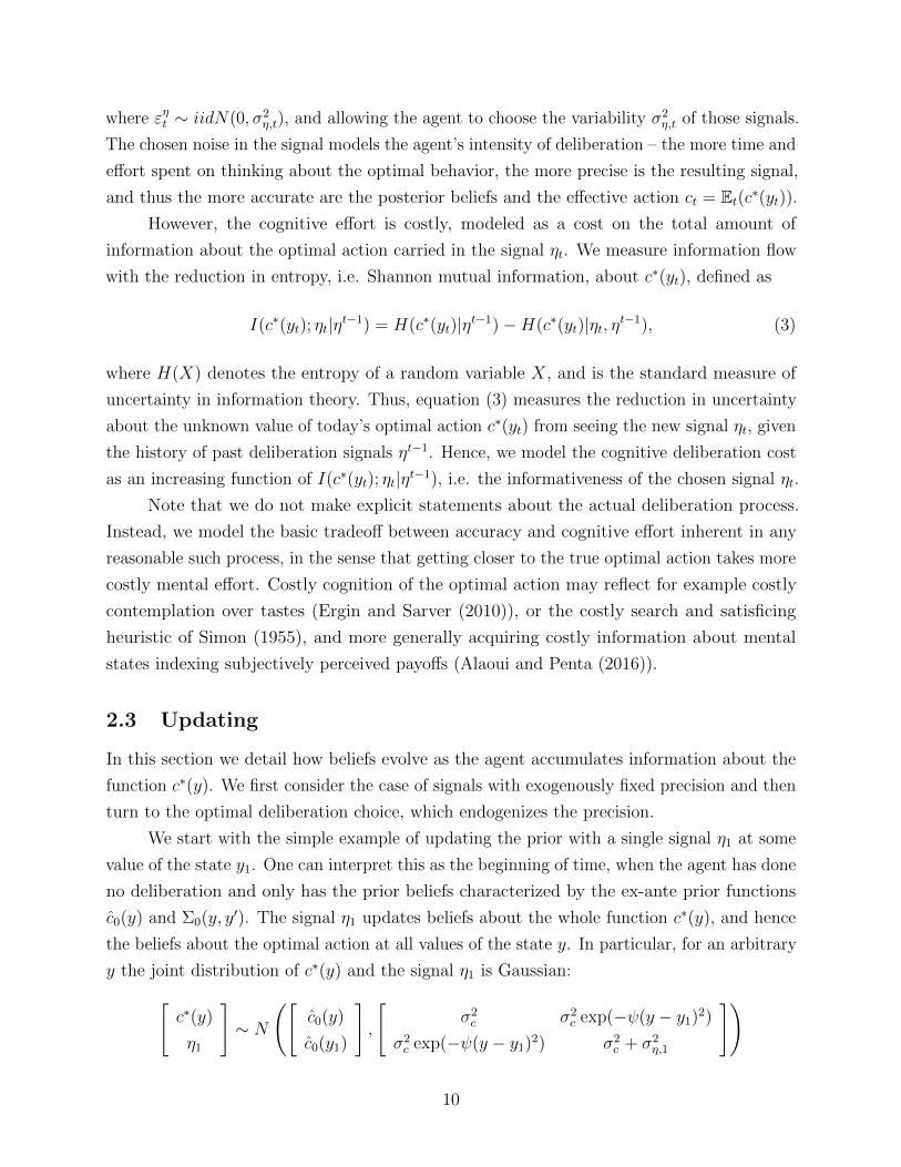
)Figure 1 illustrates both of these effects. The left panel shows the posterior mean, c1(y),
while the right panel plots the posterior variance σ21(y) as a function of y. The figure is drawn
for an example where the signal realization equals the truth, so η1 = y1. The moments are
drawn for two values of the signal error variance to showcase the effects of increased precision.
The left panel illustrates two important results. First, the effect of η1 on the conditional
beliefs about c∗(y) is state dependent. The signal has a stronger effect on the posterior mean
at values of y closer to y1, where it pulls the conditional expectation further away from the
prior and closer to the signal realization. As shown in equation (5), while information about
the optimal action at y1 is also useful about the optimal action at other y realizations, it is
most informative about realizations close to y1 – i.e. there are imperfect information spillovers
across states. Intuitively, the agent understands that he is learning about a somewhat smooth
function, and hence its value is unlikely to change drastically for a small change in y, but is
nevertheless unwilling to extrapolate information from a given signal too far.
Second, observing just one signal is useful for determining the level of the optimal
action in the neighborhood of the signal, but is only weakly informative about the shape of
the function c∗(y). In the example, the positive realization of η1 (relative to the prior c0(y1))
11
0.5 0.6 0.7 0.8 0.9 1 1.1 1.2 1.3 1.4 1.5
y
0.5
0.6
0.7
0.8
0.9
1
1.1
1.2
1.3
1.4
1.5
Con
ditio
nal e
xpec
tatio
n
Conditional Expectation of c*(y)
(a) Posterior Mean
0.5 0.6 0.7 0.8 0.9 1 1.1 1.2 1.3 1.4 1.5
y
0
0.2
0.4
0.6
0.8
1
1.2
Con
ditio
nal V
aria
nce
Conditional Variance of c*(y)
(b) Posterior Variance
Figure 1: Posterior mean and variance. Example with parameters σ2c = 1, ψ = 1, and σ2
η,0 ∈ {σ2c ,σ2c
4 }
increases the posterior mean at all values of y, but displays only a gentle slope upwards.
Increasing the signal precision helps little in that regard – as we will see, to acquire a good
grasp of the shape of the unknown function, one needs precise signals at distinct values of y.
In the right panel, we can further see that η1’s effect on uncertainty is strongest locally
to y1 – the posterior variance σ21(y) is lowest at y1, and increases away from y1. The resulting
U-shaped uncertainty reflects that beliefs about the optimal action are most precise within
the region of the state space where previously deliberated has occurred This is one of the key
features of our setup, and together with the optimal deliberation choice described below, it
helps generate the main result of an effectively non-linear policy function.
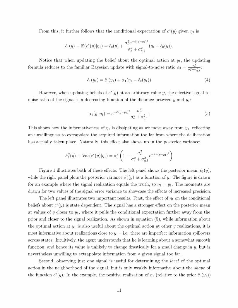
The next example adds a second signal η2, at some other state value y2. Given that
the three element vector [c∗(y), η1, η2]′ is jointly Gaussian, we apply the standard Bayesian
updating formulas to obtain the posterior mean and variance:
c2(y) = E(c∗(y)|η1, η2) = c0(y) +σ2c (e−ψ(y−y1)2 − σ2
c
σ2c+σ
2η,2e−ψ((y−y2)
2+(y2−y1)2))
(σ2c + σ2
η,1)−σ4ce−2ψ(y1−y2)2
σ2c+σ
2η,2︸ ︷︷ ︸
=α21(y;η1,η2)
(η1 − c0(y))
+σ2c (e−ψ(y−y2)2 − σ2
c
σ2c+σ
2η,1e−ψ((y−y1)
2+(y2−y1)2))
(σ2c + σ2
η,2)−σ4ce−2ψ(y1−y2)2
σ2c+σ
2η,1︸ ︷︷ ︸
=α22(y;η1,η2)
(η2 − c0(y))
12

0.5 0.6 0.7 0.8 0.9 1 1.1 1.2 1.3 1.4 1.5
y
0.5
0.6
0.7
0.8
0.9
1
1.1
1.2
1.3
1.4
1.5
Con
ditio
nal e
xpec
tatio
n
Conditional Expectation of c*(y)
(a) Posterior Mean
0.5 0.6 0.7 0.8 0.9 1 1.1 1.2 1.3 1.4 1.5
y
0
0.2
0.4
0.6
0.8
1
1.2
Con
ditio
nal V
aria
nce
Conditional Variance of c*(y)
(b) Posterior Variance
Figure 2: Posterior Mean and Variance after seeing two signals at distinct y1 6= y2. The figure illustrates an
example with parameters σ2c = 1, ψ = 1, and σ2
η,0 ∈ {σ2c ,σ2c
4 }
σ22(y) = Var(c∗(y)|η1, η2) = σ2
c
(1− (α21(y; y1, y2)e
−ψ(y−y1)2 + α22(y; y1, y2)e−ψ(y−y2)2)
),
where we define the notation α21(y; η1, η2) and α22(y; η1, η2) as the effective signal-to-noise
ratios of the two signals, η1 and η2 respectively, when updating beliefs about c∗(y).
The updating equations have much of the same features as before. In particular, signals
are more informative locally. For example if y is relatively closer to y1 than y2, the weight
put on η1 is relatively larger than on η2. Moreover, if we take the limit of yi going to infinity,
the weight on its corresponding signal ηi in the updating equation falls to zero, while the
weight on the other signal converges to the weight in the single signal case. Similarly, the
posterior variance is affected more strongly by one or the other signal, depending on whether
y is closer to y1 or to y2. We illustrate these effects in Figure 2, with the resulting posterior
mean plotted in the left panel and the posterior variance in the right panel. We assume that
η2 has the same precision as η1, and that its location, y2, is symmetric to y1 around y.
The new posterior mean c2(y) displays a steeper slope, and captures the overall shape
of the true c∗(y) better than in the single signal case. Now the agent learns that the optimal
action is relatively high for high realizations of y, but relatively low for low realizations,
leading to an upward sloping posterior. Moreover, in this case the posterior mean does not
display a bias in its overall level, since given the two symmetric signals the agent is able to
infer that the unknown function is not higher than the prior expectation on average, but
rather has a slope. Lastly, notice that increasing the precision of the signals (the red line)
now helps significantly in getting a better understanding of the shape of the underlying c∗(y).
13

In the right panel we can also see that the posterior beliefs of the agent are most precise
in the interval between y1 and y2. Interestingly, in this example the variance is the lowest not
at y1 or y2 exactly, but in between the two. This is because we have picked y1 and y2 that are
relatively close to each other, so that they are both informative for values of y in between.
More generally, as the agent accumulates information, beliefs follow the recursion
ct(y) = ct−1(y) +Σt−1(y, yt)
Σt−1(yt) + σ2η,t
(ηt − ct−1(y)) (6)
Σt(y, y′) = Σt−1(y, y
′)− Σt−1(y, yt)Σt−1(y′, yt)
Σt−1(yt) + σ2η,t
(7)
where ct(y) ≡ Et(c∗(y)|ηt) and Σt(y, y
′) ≡ Cov(c∗(y), c∗(y′)|ηt) are the posterior mean and
covariance functions. These two objects fully characterize the posterior distribution of beliefs.
Lastly, we use the notation σ2t (y) to denote the posterior variance at a given y, i.e. Σt(y, y).
2.4 Optimal deliberation
In this section we study the optimal deliberation choice and the resulting optimal signal
precision and action ct(y). We assume that the agent faces a simple linear cost in the total
information contained in ηt, and thus the information problem is22
Ut = maxσ2η,t
−WccEt(ct(yt)− c∗(yt))2 − κI(c∗(yt); ηt|ηt−1)
= maxσ2t (yt)−Wccσ
2t (yt)− κ
1
2ln
(σ2t−1(yt)
σ2t (yt)
)The second line in the above equality follows from the fact that mutual information in
a Gaussian framework is simply one half of the log-ratio of prior and posterior variances. The
parameter κ controls the marginal cost of a unit of information. For example, κ will be higher
for individuals with a higher opportunity cost of deliberation – either because they have a
higher opportunity cost of time or because their particular deliberation process takes longer
to achieve a given precision in decisions. In addition, κ would also be higher if the economic
environment facing the agent is more complex, and thus the optimal action is objectively
harder to figure out (e.g. the agent is given a more difficult math problem).
Lastly, the maximization is subject to the “no forgetting constraint”
σ2t (yt) ≤ σ2
t−1(yt),
22Assuming instead a convex cost C(I(c∗(yt); ηt|ηt−1)) in total information does not change the results.
14
which ensures that the chosen value of the noise in the signal, σ2η,t, is non-negative. Otherwise,
the agent can gain utility by “forgetting” some of his prior information.
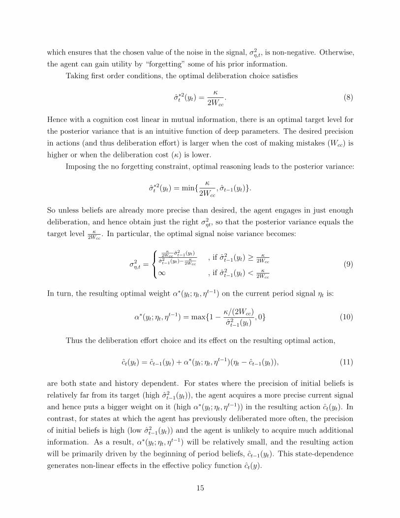
Taking first order conditions, the optimal deliberation choice satisfies
σ∗2t (yt) =κ
2Wcc
. (8)
Hence with a cognition cost linear in mutual information, there is an optimal target level for
the posterior variance that is an intuitive function of deep parameters. The desired precision
in actions (and thus deliberation effort) is larger when the cost of making mistakes (Wcc) is
higher or when the deliberation cost (κ) is lower.
Imposing the no forgetting constraint, optimal reasoning leads to the posterior variance:
σ∗2t (yt) = min{ κ
2Wcc
, σt−1(yt)}.
So unless beliefs are already more precise than desired, the agent engages in just enough
deliberation, and hence obtain just the right σ2ηt, so that the posterior variance equals the
target level κ2Wcc
. In particular, the optimal signal noise variance becomes:
σ2η,t =
κ
2Wccσ2t−1(yt)
σ2t−1(yt)−
κ2Wcc
, if σ2t−1(yt) ≥ κ
2Wcc
∞ , if σ2t−1(yt) <
κ2Wcc
(9)
In turn, the resulting optimal weight α∗(yt; ηt, ηt−1) on the current period signal ηt is:
α∗(yt; ηt, ηt−1) = max{1− κ/(2Wcc)
σ2t−1(yt)
, 0} (10)
Thus the deliberation effort choice and its effect on the resulting optimal action,
ct(yt) = ct−1(yt) + α∗(yt; ηt, ηt−1)(ηt − ct−1(yt)), (11)
are both state and history dependent. For states where the precision of initial beliefs is
relatively far from its target (high σ2t−1(yt)), the agent acquires a more precise current signal
and hence puts a bigger weight on it (high α∗(yt; ηt, ηt−1)) in the resulting action ct(yt). In
contrast, for states at which the agent has previously deliberated more often, the precision
of initial beliefs is high (low σ2t−1(yt)) and the agent is unlikely to acquire much additional
information. As a result, α∗(yt; ηt, ηt−1) will be relatively small, and the resulting action
will be primarily driven by the beginning of period beliefs, ct−1(yt). This state-dependence
generates non-linear effects in the effective policy function ct(y).
15

2.5 Comparison with imperfect perception of the objective state
The typical approach in the literature that analyzes optimal allocation of attention is to
focus on imperfect perception of the state rather than the policy function. In our setup, this
consists in assuming knowledge of the optimal policy c∗(y) = y, but imperfect observability
of the state yt. Learning about yt proceeds similarly, by observing unbiased signals
ηt = yt + εηt ,
where the signal noise variance is σ2η,t. The conditional expectation of yt becomes:
yt ≡ Et(yt) = y +σ2y
σ2y + σ2
η,t
(ηt − y). (12)
The optimal action under the quadratic loss is then just the above conditional expectation
of yt, since agents know that c∗(yt) = yt. Moreover, if the cognition cost is similarly linear in
the Shannon information of the signal ηt, it results in the maximization problem:
U = maxσ2y,t
−Wccσ2y,t − κ
1
2ln
(σ2y,t−1
σ2y,t
),
where we denote the posterior variance of yt as σ2y,t ≡ Var(yt|ηt). The cost of information is
also linear in mutual information, but the marginal cost κ could be different than κ, since
this captures information flow of a different activity – paying attention to an unknown state.
The first order conditions again imply a target level for the posterior variance:
σ∗2y,t =κ
2Wcc
, ∀t (13)
Thus, the resulting optimal signal-to-noise ratio, given the “no forgetting constraint”, is
α∗y = max{1− κ/(2Wcc)
σ2y
, 0}, ∀t (14)
The key difference between the optimal α∗y in equation (14) and that of our benchmark
framework, given by equation (10), is that in our model the prior uncertainty σ2t−1(yt), and
in turn the resulting signal to noise ratio α∗(y; ηt, ηt−1), are state and history dependent.
Instead, here α∗y is the same for all current and past realizations of the state yt.23 The state
23The assumption that yt is iid over time makes the optimal attention solution particularly simple, but thefact that it is not state or history dependent is a more general result. If yt was persistent, then we wouldsimply substitute the steady state Kalman filter second moments for σ2
y in the updating equations.
16

and history dependence of the deliberation choice is a fundamental feature of our setup.
Because the agent is not learning about the current realization of the state yt, but about the
optimal policy function c∗(y), deliberation at different past values of the state carry different
amount of information about the optimal action at today’s state yt.
Our reasoning setup includes a special case that delivers the same qualitative features
as learning about the objective state. In the first period of reasoning in our model (i.e. time
1), the prior uncertainty is neither state- nor history- dependent since σ20(y) = σ2
c , ∀y. Hence,
the optimal signal-to-noise ratio in that period is qualitatively similar to equation (14),
α∗(y; η1) = max{1− κ/(2Wcc)
σ2c
, 0}, (15)
with no state or history dependence. The first period of learning is special in our reasoning
setup because it is the only instance where the agent has accumulated no previous information,
and hence the remaining uncertainty is the same at all values of the state. As soon as
information starts accumulating, however, the implications of the two models diverge.
The general relation to models of errors in actions can also be made by connecting to
the control cost literature. More specifically, the deliberation choice in our setup can be
rewritten ‘as if’ it is a control cost problem where the agent has a ‘default’ distribution of
actions, conditional on the state, and chooses a current distribution, subject to a cost that is
increasing in the distance between the two distributions, as measured by relative entropy.24
In our model, the default distribution is the beginning of period belief over the unknown
c∗(yt) and the current distribution is the posterior belief after seeing ηt. While many models
of imperfect actions, including those generated from known policy functions but imperfect
perception of objective states, fit in such an ‘as if’ control cost interpretation, the differential
property of our model is in the particular endogenous dynamics of the ‘default’ distribution.25
3 Ergodic Distribution of Beliefs and Actions
Since the deliberation choice is history dependent we focus on analyzing the ergodic behavior
of our agent. In this section, we characterize the typical optimal deliberation choice and
resulting effective policy function ct(y) after having seen and previously deliberated at a long
history of state realizations. In the following Section 4, we study how a change in deliberation
and resulting information about the unknown c∗(y) propagates into subsequent actions.
24The control cost approach appears for example in game theory (see Van Damme (1987)) and the entropybased cost function is studied in probabilistic choice models such as Mattsson and Weibull (2002).
25Matejka and McKay (2014) and Matejka et al. (2017) show the mapping between an entropy-basedattention cost and a control problem leading to logit choices in static and dynamic environments, respectively.
17
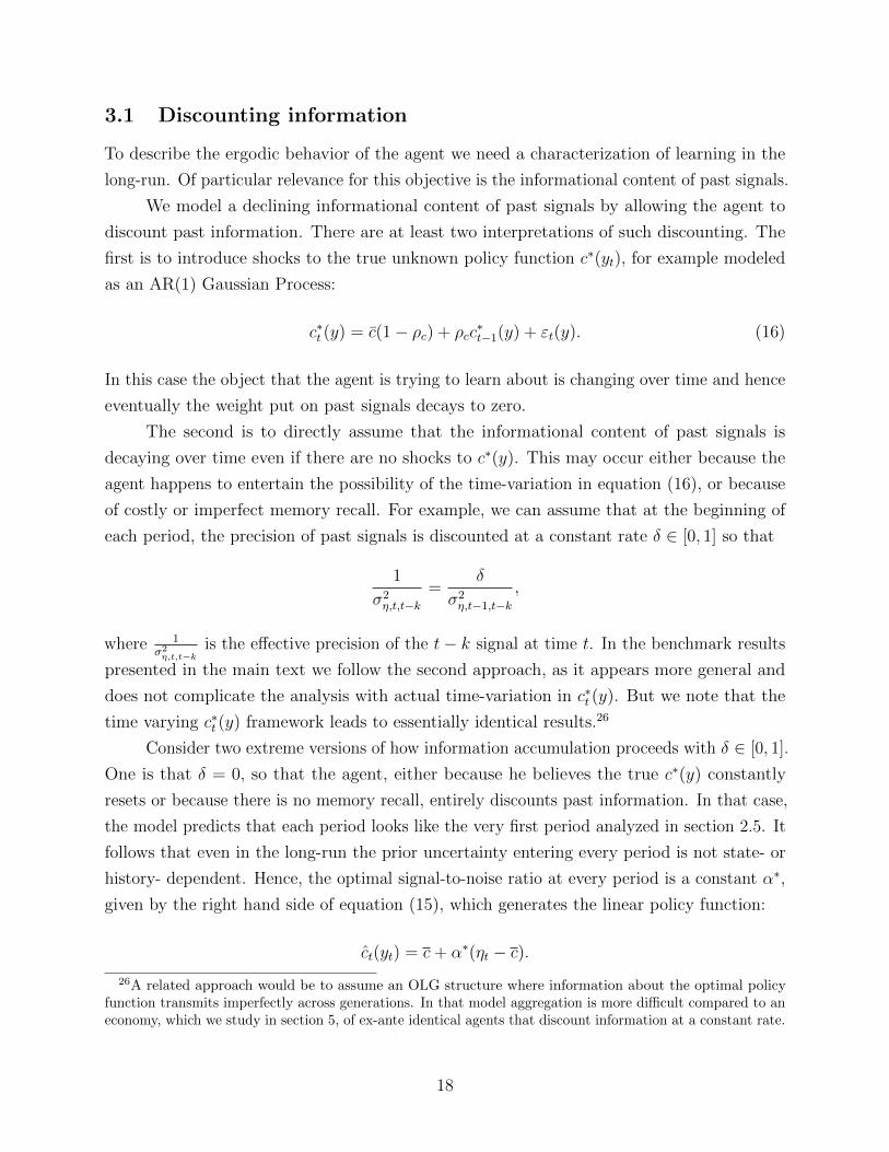
3.1 Discounting information
To describe the ergodic behavior of the agent we need a characterization of learning in the
long-run. Of particular relevance for this objective is the informational content of past signals.
We model a declining informational content of past signals by allowing the agent to
discount past information. There are at least two interpretations of such discounting. The
first is to introduce shocks to the true unknown policy function c∗(yt), for example modeled
as an AR(1) Gaussian Process:
c∗t (y) = c(1− ρc) + ρcc∗t−1(y) + εt(y). (16)
In this case the object that the agent is trying to learn about is changing over time and hence
eventually the weight put on past signals decays to zero.
The second is to directly assume that the informational content of past signals is
decaying over time even if there are no shocks to c∗(y). This may occur either because the
agent happens to entertain the possibility of the time-variation in equation (16), or because
of costly or imperfect memory recall. For example, we can assume that at the beginning of
each period, the precision of past signals is discounted at a constant rate δ ∈ [0, 1] so that
1
σ2η,t,t−k
=δ
σ2η,t−1,t−k
,
where 1σ2η,t,t−k
is the effective precision of the t− k signal at time t. In the benchmark results
presented in the main text we follow the second approach, as it appears more general and
does not complicate the analysis with actual time-variation in c∗t (y). But we note that the
time varying c∗t (y) framework leads to essentially identical results.26
Consider two extreme versions of how information accumulation proceeds with δ ∈ [0, 1].
One is that δ = 0, so that the agent, either because he believes the true c∗(y) constantly
resets or because there is no memory recall, entirely discounts past information. In that case,
the model predicts that each period looks like the very first period analyzed in section 2.5. It
follows that even in the long-run the prior uncertainty entering every period is not state- or
history- dependent. Hence, the optimal signal-to-noise ratio at every period is a constant α∗,
given by the right hand side of equation (15), which generates the linear policy function:
ct(yt) = c+ α∗(ηt − c).26A related approach would be to assume an OLG structure where information about the optimal policy
function transmits imperfectly across generations. In that model aggregation is more difficult compared to aneconomy, which we study in section 5, of ex-ante identical agents that discount information at a constant rate.
18
This extreme is a special case of our setup that replicates the qualitative features of
imperfect perception about the objective state (see section 2.5). Importantly, there is no
non-linearity in the effective policy function, nor information propagation through time.
A second extreme case is given by δ = 1, so that the agent does not discount at all past
information. In this case the important characteristic of the limiting beliefs is that as time
passes, it becomes increasingly likely that the agent stops reasoning altogether. Recall that
each time the agent decides to reason, i.e. when σ2η,t <∞, the amount of reasoning is chosen
so that the resulting posterior variance σt(yt) equals the optimal target level κ/(2Wcc) in
equation (8). Without discounting past information, it follows that the perceived uncertainty
at state values in the neighborhood of past realizations yt would typically be either equal
or even smaller than that target, since there are information spillovers across states. As
information accumulates through time, further learning in the neighborhood of past state
realizations stops altogether. In particular, the agent chooses not to reason in period t, i.e.
sets σ2η,t =∞, with a probability that converges to one as t goes to infinity.
Therefore, there are two important implications of setting δ = 1. First, even if further
reasoning eventually stops, the beliefs still do not converge to c∗(y) because the optimal
posterior variance is positive, since reasoning is costly. Second, the flow of new information
eventually stops almost everywhere, and the agent simply acts according to the prior ct−1(y).
Moreover, the limiting beliefs of the agent will depend on specific signals accumulated in the
very distant past, hence there is no ergodic distribution of beliefs as t goes to infinity.
We find the behavioral assumptions and implications of not discounting past information
as implausible. Such a view relies on the extreme assumptions of perfect memory recall and
no perceived structural changes. Furthermore, this view implies that agents do not further
adjust their beliefs as the economy evolves through time, but dogmatically use their priors.
We relax the extreme assumptions of either full or no discounting of past information
and study the ergodic distribution of beliefs resulting for intermediate values of δ ∈ (0, 1). In
that case, there will be further reasoning even in the long-run and the agents’ beliefs will
respond to new information, features that we find plausible. Moreover, there is a well defined
long-run ergodic distribution of beliefs and resulting actions, which we characterize next.
3.2 Properties of the ergodic distribution of beliefs
To obtain the ergodic distribution, we simulate the economy for 100 times, each of a length
of 1000 periods, where in each period we draw a new value of the state and the agent makes
optimal deliberation choices given the history of signals. Then we consider the average
resulting prior conditional variance, optimal deliberation choice and effective policy function
19

0.5 0.6 0.7 0.8 0.9 1 1.1 1.2 1.3 1.4 1.5
y
0.2
0.25
0.3
0.35
0.4
0.45
0.5
0.55
Con
ditio
nal V
aria
nce
(a) Prior Conditional Variance
0.5 0.6 0.7 0.8 0.9 1 1.1 1.2 1.3 1.4 1.5
y
0
0.1
0.2
0.3
0.4
0.5
0.6
(b) Optimal Signal-to-Noise ratio
Figure 3: Ergodic Uncertainty – beginning of period prior variance and the resulting optimal signal-to-noise ratio after 1000 periods of optimal deliberation. The figure illustrates an example with parametersWcc = 1, κ = 0.5, σ2
c = 1, ψ = 1, and δ = 0.9.
as a function of possible state realizations y.
In the left panel of Figure 3 we plot the mean of the ergodic distribution of the prior
conditional variance of beliefs (i.e. the conditional variance coming into a typical period t),
σss0 (y) =
∫Var(c(y)|ηt−1)dF (ηt−1),
where dF (ηt−1) is the ergodic distribution of histories of optimal past signals. In the right
panel we plot the resulting ergodic optimal signal-to-noise ratio for the new signal, αss(y).
The ergodic prior conditional variance has a characteristic U-shape, and is lowest around
the mean of the distribution of states, y. The reason is that this is the part of the state
space where the agent has deliberated at most often in the past, and hence most of the past
signals η are for values of y near their mean. Intuitively, coming into the typical period, the
agent feels most certain about what is the optimal thing to do for state realizations near
their mean, and is increasingly less certain about what to do if the state happens to be far
from y. Moreover, notice that there is an interval of y values where the ergodic prior variance
is in fact below the target level κ2Wcc
. This occurs because while no individual signal ever
lowers the conditional variance below the optimal level by itself, the combined effects of the
large concentration of signals around y and the accompanying information spillovers do so.
The U-shape in the ergodic prior variance leads to a similar shape in the optimal signal
to noise ratio αss(y) – it is the lowest for values of the state close to y, and grows larger for
20

0.6 0.7 0.8 0.9 1 1.1 1.2 1.3 1.4
y
0
0.5
1
1.5
2
2.5
3
3.5
4
(a) Distribution of incidence of past reasoning signals
0.6 0.7 0.8 0.9 1 1.1 1.2 1.3 1.4
y
0.01
0.02
0.03
0.04
0.05
0.06
0.07
0.08
0.09
0.1
0.11
(b) Average precision of past signals at a given y
Figure 4: Ergodic distribution of reasoning signals and associated precision, after 1000 periods of optimaldeliberation. The figure illustrates an example with parameters Wcc = 1, κ = 0.5, σ2
c = 1, ψ = 1, and δ = 0.9.
realizations of y further out. The reason is that in order to achieve the optimal precision of
posterior beliefs, the agent has to do less additional thinking for state realizations around the
mean, as there the initial beliefs are already quite precise. Thus, the ergodic deliberation
choice is akin to salient thinking – the agent finds it optimal to reason harder at more unusual
realizations of the state. Not because those tend to “stand out” more, but because the agent’s
prior understanding of the optimal action in that part of the state space is worse.
In Figure 4 we illustrate the properties of the ergodic distribution of past reasoning
signals, F (ηt−1). In the left panel we plot the ergodic distribution of y realizations for which
the agent has deliberated in the past. Note that the agent does not necessarily deliberate (and
thus obtain an informative signal) in every period – costly deliberation is only triggered if the
prior uncertainty is relatively large, as evidenced by the right panel of Figure 3. Nevertheless,
the ergodic distribution of the incidence of reasoning is quite similar to the distribution of y.
Still, this is not the whole story, since we just saw that the optimal signal precision is state
dependent. For this purpose, the right panel of Figure 4 plots the ergodic mean precision of
optimal signals at each value of the state y. Unsurprisingly, we see that individual signals
are most precise for values of y further away from y, and the least precise right around y.
In other words, the agent tends to have deliberated most often for realizations around y,
but the typical deliberation in that region has been relatively imprecise. Intuitively, the agent
spends a lot of time near y, and ends up reasoning there often. But since the typical history
is already quite informative about c∗(y) in that region, there is no need for much additional
21

0.5 0.6 0.7 0.8 0.9 1 1.1 1.2 1.3 1.4 1.5
y
0.5
0.6
0.7
0.8
0.9
1
1.1
1.2
1.3
1.4
1.5
Act
ion
Figure 5: Ergodic Policy Function. The figure plots the ergodic average action, computed from a cross-sectionof 100 agents and 1000 time periods, with parameters Wcc = 1, κ = 0.5, σ2
c = 1, ψ = 1, and δ = 0.9
reasoning effort, hence the typical signal in that region is imprecise. At the same time, the
agent tends to see and deliberate at unusual y values more rarely, but conditional on doing so,
invests a significant amount of effort, and thus obtains more precise signals. As a result, the
typical history of deliberations delivers a large concentration of relatively imprecise signals
around y, and fewer but more individually precise signals at values further away from y.
3.3 Non-linearity in ergodic policy function
The red line in Figure 5 plots the resulting mean ergodic policy function,
css(y) ≡ css0 (y) + αss(y)(η(y)− css0 (y)), (17)
where η(y) = c∗(y) is the new mean signal at y, and css0 (y) is the mean ergodic prior belief:
css0 (y) ≡∫E(c∗(y)|ηt−1)dF (ηt−1).
The key emerging property of the ergodic policy function is that it is non-linear, even
though the underlying optimal policy function (c∗(y)) is linear. The non-linearity is a result
of the fact that the optimal deliberation choice is state dependent, and hence the optimal
signal to noise ratio αss(y) is a non-constant function of y. In particular, we have seen that
the ergodic prior uncertainty σss0 (y) is U-shaped, hence the agent finds it optimal not to
reason much for realizations of y near y. Thus in that region the optimal αss(y) is low and
22
so the action is primarily driven by the ergodic prior mean css0 (y). On the other hand, at
more unusual state realizations y, the agent’s prior beliefs are more uncertain, prompting the
agent to invest more costly cognitive effort, and obtain a more precise signal. This leads to
a higher αss(y), and hence for those values of y the agent’s beliefs and resulting action are
closer to the actual signal realization. As a result of the changing weight attached to the
revision in his prior beliefs, αss(y), the ergodic policy function of the agent is non-linear.
In our benchmark setup, this non-linearity generates both inertia and salience-like
effects in the ergodic policy function, as it is relatively flat in the middle, and more responsive
in the tails. This is due to the interaction of the U-shaped ergodic signal-to-noise ratio αss(y)
and the endogenous shape of the ergodic prior belief c0(y). At state realizations around
y, the agent does not engage in much further deliberation and his action is mainly driven
by the relatively flat prior belief css0 (y) (see yellow dashed line). However, at more unusual
realizations of y the action puts a heavier weight on the new, informative signal η, which
deviates from the ergodic prior beliefs and leads to a stronger response.
The shape of the ergodic prior belief css0 (y) is due to the characteristics of the endogenous
distribution of past reasoning signals F (ηt−1). The majority of the “fresh” signals in the
agent’s memory are from around y, where the agent has seen seen numerous, but individually
imprecise signals (Figure 4). The large number of imprecise signals helps pin down the
average level of c∗(y), but not its shape. The agent’s ergodic prior beliefs are still somewhat
upwards sloping (as is the true policy c∗(y)) because of the fewer, but more precise signals
further out in the tails, but their effect is dominated by the fact that the bulk of the prior
information has come in the form of many, but imprecise signals. Intuitively, the agent has
a good grasp of the overall level of the optimal action around y, so finds it unnecessary to
spend much extra effort to understand how the optimal action varies with small changes in y.
It is also worth nothing that this is the typical or average ergodic behavior of the agent.
At any given point in time, agents in this economy behave differently due to having seen
different particular histories of signals. These histories lead to effective policy functions that
are either more or less upward sloping than the average, and could also exhibit a number of
other types of non-linearity. We discuss such heterogeneity in more detail in Section 5.
Lastly, the purple line plots the ergodic policy function of an agent who observes the
state y imperfectly, but knows the optimal policy function c∗(y). The key property of that
policy function is that it is linear, since it inherits the known form of c∗(y). It displays a
constant under-reaction to changes in y, because the only mistake the agent is making is in
tracking the true value of y, and is (on average) slow in recognizing changes.
23
0.5 0.6 0.7 0.8 0.9 1 1.1 1.2 1.3 1.4 1.5
y
0.5
0.6
0.7
0.8
0.9
1
1.1
1.2
1.3
1.4
1.5
(a) Changing κ and ψ
0.5 0.6 0.7 0.8 0.9 1 1.1 1.2 1.3 1.4 1.5
y
0.5
0.6
0.7
0.8
0.9
1
1.1
1.2
1.3
1.4
1.5
(b) Changing δ
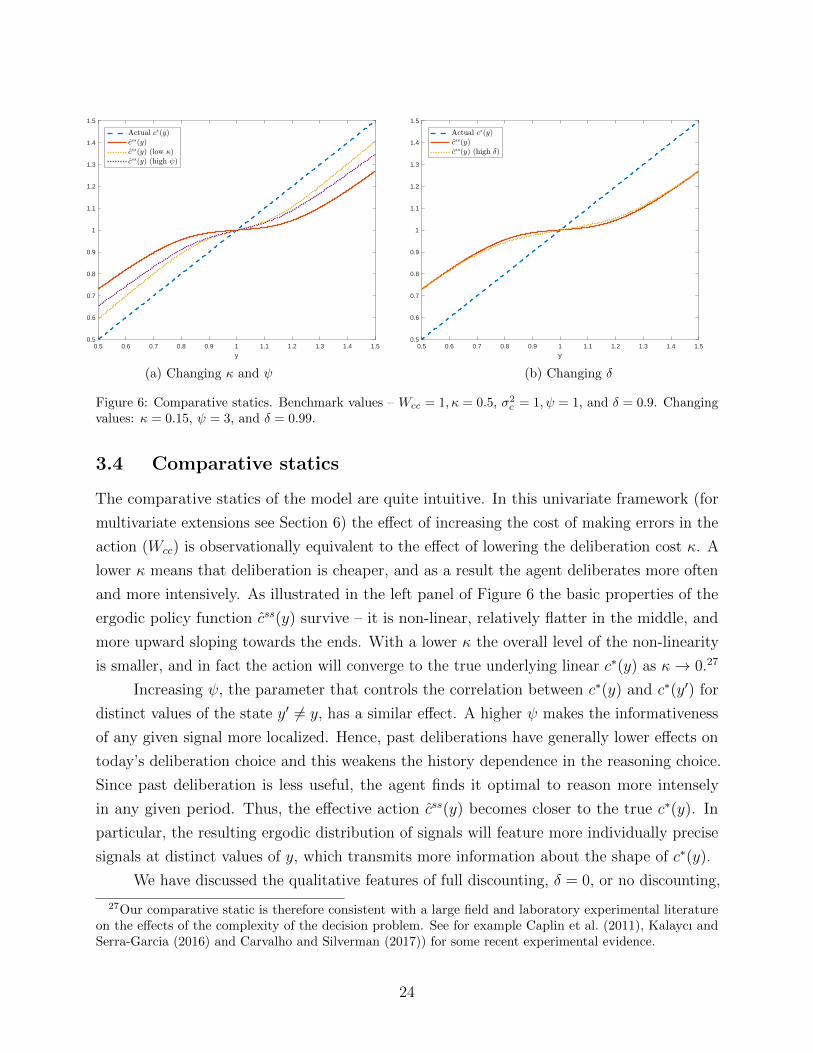
Figure 6: Comparative statics. Benchmark values – Wcc = 1, κ = 0.5, σ2c = 1, ψ = 1, and δ = 0.9. Changing
values: κ = 0.15, ψ = 3, and δ = 0.99.
3.4 Comparative statics
The comparative statics of the model are quite intuitive. In this univariate framework (for
multivariate extensions see Section 6) the effect of increasing the cost of making errors in the
action (Wcc) is observationally equivalent to the effect of lowering the deliberation cost κ. A
lower κ means that deliberation is cheaper, and as a result the agent deliberates more often
and more intensively. As illustrated in the left panel of Figure 6 the basic properties of the
ergodic policy function css(y) survive – it is non-linear, relatively flatter in the middle, and
more upward sloping towards the ends. With a lower κ the overall level of the non-linearity
is smaller, and in fact the action will converge to the true underlying linear c∗(y) as κ→ 0.27
Increasing ψ, the parameter that controls the correlation between c∗(y) and c∗(y′) for
distinct values of the state y′ 6= y, has a similar effect. A higher ψ makes the informativeness
of any given signal more localized. Hence, past deliberations have generally lower effects on
today’s deliberation choice and this weakens the history dependence in the reasoning choice.
Since past deliberation is less useful, the agent finds it optimal to reason more intensely
in any given period. Thus, the effective action css(y) becomes closer to the true c∗(y). In
particular, the resulting ergodic distribution of signals will feature more individually precise
signals at distinct values of y, which transmits more information about the shape of c∗(y).
We have discussed the qualitative features of full discounting, δ = 0, or no discounting,
27Our comparative static is therefore consistent with a large field and laboratory experimental literatureon the effects of the complexity of the decision problem. See for example Caplin et al. (2011), Kalaycı andSerra-Garcia (2016) and Carvalho and Silverman (2017)) for some recent experimental evidence.
24

δ = 1, in subsection 3.1. We now describe the effects of changing the discounting parameter
within these two extreme versions. For a fixed sequence of past signals ηt−1, increasing δ
would increase the overall informativeness of the signals, and lead to a lower optimal level of
current deliberation. Since past signals are more informative the agent chooses to reason less
at any given period. As a result, at the new ergodic distribution with a higher δ the agent
has an effectively longer typical history of signals, but individual signals tend to have lower
precision. In turn, the effective residual uncertainty and the resulting policy function are
similar to the case of lower δ, as exemplified by the right panel of Figure 6, for δ = 0.99.
Lastly, we consider changing the ex-ante prior mean function c0(y). Importantly, c0(y)
has no effect on the deliberation choice of the agent, or the weight put on the reasoning
signals in updating beliefs. The deliberation choice and the updating process depend only
on second moments, and those are unaffected by c0(y). Thus, the main results about the
U-shaped ergodic uncertainty, salient thinking and the non-linear ergodic policy function
remain unchanged. Still, changing c0(y) would serve to tilt the resulting posterior beliefs,
as a non-constant prior mean function implies that the agent has some a priori belief about
c∗(y) that would apply over and above the information extracted from the reasoning signals
η. It is one way, for example, to model ex-ante biases in agent behavior.
To illustrate, consider the possibility that c0(y) is given by the linear function
c0(y) = c+ b0(y − y). (18)
Figure 7 plots two such cases, one where b0 < 1 so that c0(y) is flatter than the truth, and
one where b0 > 1 and c0(y) is steeper than c∗(y). The main insight that the ergodic policy
function is non-linear, and that its shape is different close to y, as opposed to out in the tails,
remains unchanged. This basic feature is due to the state-dependent deliberation choice that
resembles salient thinking, a result that does not depend on c0(y). In the left panel (b0 < 1),
the policy is qualitatively similar to our benchmark case – relatively flatter in the middle, and
steeper in the tails. The right panel, however, is the opposite – the ergodic policy is steeper in
the middle, and flatter in the tails. In this case, the ergodic prior mean css0 (y) is steeper than
the truth (although less steep than the ex-ante prior c0(y)), and hence the strong revisions in
beliefs that happen for tail y realizations actually flatten the posterior mean.
While it is straightforward to incorporate different ex-ante prior means c0(y), we find it
conceptually unappealing because it represents extra information about the optimal policy
that the agent receives for free. The basic premise of the model is to make deliberation and
information about c∗(y) subject to costly reasoning effort, hence playing with the ex-ante
prior would represent back-door information flows. Moreover, the most empirically relevant
25

0.5 0.6 0.7 0.8 0.9 1 1.1 1.2 1.3 1.4 1.5
y
0.5
0.6
0.7
0.8
0.9
1
1.1
1.2
1.3
1.4
1.5
Act
ion
(a) Flatter than true c∗(y) ( b0 = 1/3)
0.5 0.6 0.7 0.8 0.9 1 1.1 1.2 1.3 1.4 1.5
y
-0.5
0
0.5
1
1.5
2
2.5
Act
ion
(b) Steeper than true c∗(y) ( b0 = 3)
Figure 7: Different prior mean function c0(y). Benchmark values – Wcc = 1, κ = 0.5, σ2c = 1, ψ = 1, and
δ = 0.9. Changing values: b0 ∈ { 13 , 3} in equation (18).
case is perhaps the one where b0 < 1, since it implies inertia for “familiar” values of the
state, and salience like effects for others. This conforms with experimental evidence, and also
can help explain a number of other features of the macro data, as we detail in the next few
sections. Thus, the best parsimonious model would appear to be b0 = 0.
4 Propagation of Information
We have described the properties of the ergodic distribution of beliefs and actions. In this
section we study the typical propagation of information so as to analyze the time-series
patterns of actions. The key emerging property is that reasoning about the function c∗(y)
endogenously leads to persistence in the first and second moment of actions.
4.1 Persistent actions
We focus first on the persistence of the conditional mean belief about the optimal action,
following the recursion in equation (6), with ergodic properties described in section 3.3.
4.1.1 Impulse response
Let us analyze a change in the state from y to some particular realization yt. To understand
the effect on beliefs it is useful to separate its mechanisms into impact and then propagation.
26

The initial effect of the shock appears in the revision of beliefs term in the ergodic
policy function css(y) in equation (17). The weight put on the new information obtained at
yt, αss(yt), depends on the ergodic prior uncertainty, while the ergodic prior mean determines
the perceived innovation ηt − css0 (yt). For example, in the benchmark case shown in Figure
5, where the ergodic prior mean css0 (y) is flatter than the true c∗(y), the sign of the average
perceived innovation c∗(yt)− css0 (yt) is given by the sign of the true average innovation yt − y.
The propagation of the new information depends crucially on the knowledge spillovers
implied by our learning framework. For a large enough value of ψ, the agent’s prior is that a
signal about c∗(yt) is essentially useless about c∗(y) at some y 6= yt. In that case, the relevant
effect of the new signal is to update beliefs only about the optimal action at yt. But since the
probability of a future realization being very near to that specific value of yt is close to zero,
there are no significant persistent effects. In contrast, for a smaller ψ, the signal obtained at
yt shifts beliefs about the entire unknown function c∗(y). As new states realize after period t,
this shift in beliefs persists before it converges back to the ergodic belief css0 (y). In this case,
a signal about the optimal action at yt is likely to have persistent effects on the resulting
actions, even if the objective state is iid.
Consider a graphical representation of the impulse response function of the agent’s
effective action ct.28 The blue solid line in the left panel of Figure 8 plots the impulse response
starting from t for a value of the state yt = y − 2σy for the benchmark parametrization. The
initial effect on the action can be read off directly from the ergodic policy function css(yt)
discussed in section 3.3. On impact, the action incorporates about 25% of the change in the
state, dropping by 0.05 compared to the reduction of 0.2 in yt.
While such underreaction appears more generally in models of partial attention to the
objective states, an important additional property of our model is the resulting propagation.
As described above, the negative shock to yt results in a negative perceived innovation about
the optimal action at yt. Due to the knowledge spillovers, this innovation affects beliefs
about the unknown policy function not only at yt but even further away from it, producing a
persistently lower average action following the shock.
The left panel illustrates the role of parameters in driving the propagation. The response
on impact is stronger and there is less persistence when the cognition cost is lower (‘low
κ’, dotted yellow line), or when the signal at yt is less informative at other states (‘high ψ’,
dashed orange line), because in both cases the agent is more likely to reason harder at any
given period. Hence the initial impact is greater, but the value of this information declines
28Given the non-linear nature of our model we compute a generalized impulse response function to aparticular realization of the state yt as IRFj(yt) = E(ct+j |yt) − E(ct+j |yt = y). Moreover, to isolate thetypical effects, we set the signal realization equals to its average value, so that εt = 0 in this analysis.
27

2 4 6 8 10 12 14 16 18
time
-12
-10
-8
-6
-4
-2
0P
erce
nt d
evia
tion
from
mea
n
(a) Alternative parameterizations
5 10 15 20 25 30 35 40
time
-10
-8
-6
-4
-2
0
Per
cent
dev
iatio
n fr
om m
ean
(b) Alternative shock realizations
Figure 8: Impulse response function. The figure plots the typical path of the action following an innovationof yt = y − 2σy. The figure illustrates an example with parameters Wcc = 1, κ = 0.5, σ2
c = 1, ψ = 1, andδ = 0.9. In the left panel we change parameters to κ = 0.1, ψ = 5 and δ = 1, respectively. In the right panelwe change persistence to ρy = .9 (dashed line), or we feed in future values of yt+j that always equal to y(starred line), or set the current shock to yt = y − 3σy (dotted line).
quickly as more relevant new information comes in the following periods. When there is no
discounting of past information (‘δ = 1’, starred purple line), the agent has accumulated so
much information that he does not further deliberate and instead only uses the ergodic prior
mean at yt to inform his action ct. The lack of further updating leads to no persistent effects.
The right panel of Figure 8 illustrates the strong non-linearity by plotting three
alternative assumptions on the shock realizations. First, in the dotted orange line, the state
realization is more unusual (yt = y − 3σy). On impact, the action now incorporates about
33% of the change in the state, dropping by 0.11 compared to the reduction of 0.3 in yt. The
larger proportional reduction than in the baseline case reflects the more pronounced steepness
of the ergodic policy for tail yt realizations. Moreover, since the state is now more unusual,
the agent chooses to reason more intensely. This results in a larger weight applied to the new
signal and stronger updating about the whole function, and therefore longer persistence.
Second, in the starred purple line, we compute the impulse response as in a linear model
by ignoring the distribution of future states and instead feeding in yt+j = y for all j > 0.
Since the agent would now constantly see y and hence not reason any further, the effect of the
initial update at yt would be longer lasting. In contrast, with shocks to yt+j , it is more likely
that some of those realizations trigger reasoning. The larger chance of future reasoning on
average decreases the weight put in the future on the signal at yt, generating less persistence.
Finally, consider the case of an ex-ante prior mean c0(y) that is not constant as in our
28
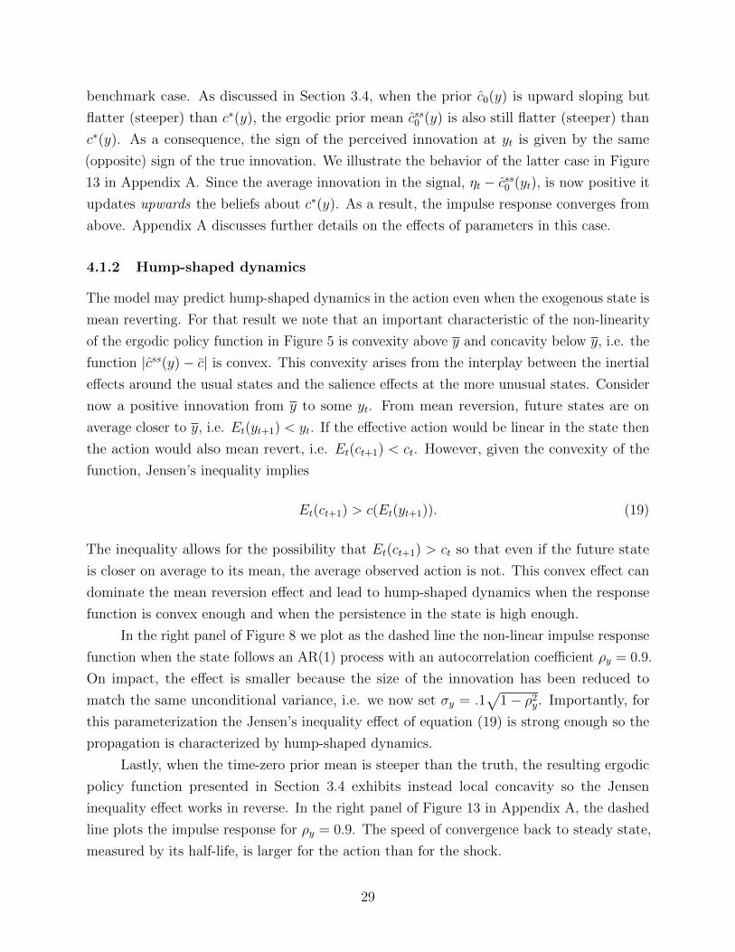
benchmark case. As discussed in Section 3.4, when the prior c0(y) is upward sloping but
flatter (steeper) than c∗(y), the ergodic prior mean css0 (y) is also still flatter (steeper) than
c∗(y). As a consequence, the sign of the perceived innovation at yt is given by the same
(opposite) sign of the true innovation. We illustrate the behavior of the latter case in Figure
13 in Appendix A. Since the average innovation in the signal, ηt − css0 (yt), is now positive it
updates upwards the beliefs about c∗(y). As a result, the impulse response converges from
above. Appendix A discusses further details on the effects of parameters in this case.
4.1.2 Hump-shaped dynamics
The model may predict hump-shaped dynamics in the action even when the exogenous state is
mean reverting. For that result we note that an important characteristic of the non-linearity
of the ergodic policy function in Figure 5 is convexity above y and concavity below y, i.e. the
function |css(y)− c| is convex. This convexity arises from the interplay between the inertial
effects around the usual states and the salience effects at the more unusual states. Consider
now a positive innovation from y to some yt. From mean reversion, future states are on
average closer to y, i.e. Et(yt+1) < yt. If the effective action would be linear in the state then
the action would also mean revert, i.e. Et(ct+1) < ct. However, given the convexity of the
function, Jensen’s inequality implies
Et(ct+1) > c(Et(yt+1)). (19)
The inequality allows for the possibility that Et(ct+1) > ct so that even if the future state
is closer on average to its mean, the average observed action is not. This convex effect can
dominate the mean reversion effect and lead to hump-shaped dynamics when the response
function is convex enough and when the persistence in the state is high enough.
In the right panel of Figure 8 we plot as the dashed line the non-linear impulse response
function when the state follows an AR(1) process with an autocorrelation coefficient ρy = 0.9.
On impact, the effect is smaller because the size of the innovation has been reduced to
match the same unconditional variance, i.e. we now set σy = .1√
1− ρ2y. Importantly, for
this parameterization the Jensen’s inequality effect of equation (19) is strong enough so the
propagation is characterized by hump-shaped dynamics.
Lastly, when the time-zero prior mean is steeper than the truth, the resulting ergodic
policy function presented in Section 3.4 exhibits instead local concavity so the Jensen
inequality effect works in reverse. In the right panel of Figure 13 in Appendix A, the dashed
line plots the impulse response for ρy = 0.9. The speed of convergence back to steady state,
measured by its half-life, is larger for the action than for the shock.
29
4.2 Persistence of volatility of actions
A general property of our model is that particular realizations of the objective state change
the actions’ responsiveness to those realizations as well as to subsequent ones. For an
econometrician using a standard model, such changes may look like structural shifts in
parameters. In particular, in this section we show how our model predicts endogenous
time-variation in the volatility of actions. To explain this variation, an econometrician may
conclude that there are shocks to the volatility of the objective state, i.e. changes in σy.
4.2.1 Volatility clustering
We illustrate how the model generates clusters of volatility through the following experiment.
Once the economy reaches its ergodic distribution, at some point t we feed in a randomly
drawn sequence of states of length s. We directly affect the variability of that vector by
multiplying it by a scalar V. Denote the resulting vector of chosen actions in this first stage
as a1. At time t+ s, we feed in another random sequence of states of length s, also multiplied
by V. Collect the vector of chosen actions in this second stage as a2. We simulate repeatedly
over the draws, vary V and report σ(a2), the standard deviation of actions in the vector a2,
compared to the action vector a1, σ(a1). Notice that, on average, the standard deviation of
the states generating the two actions is the same, given by V σy.
At the ergodic distribution there are two main implications for actions when observing
a sample with more volatile states. One is a direct effect through which the actions are also
more volatile, since they respond to the observed states. More importantly, there is a second,
propagating effect arising from the fact that given more unusual states, the agent chooses
to reason more intensely. By reasoning, the agent obtains more informative signals about
the unknown policy function. In our benchmark case, the more intense reasoning leads, on
average, to an updated belief at t + s − 1 characterized by stronger responses to y. This
updated belief generates more variable actions starting at t+ s, as the belief converges back
to the ergodic css0 (y). Therefore, the more intense reasoning, stimulated by more variable
state realizations, leads to an endogenous persistent increase in the variability of actions.
In our experiment we therefore find that the ratio σ(a2)/σ(a1) is increasing in V , or,
put differently, it is increasing in σ(a1), since the latter is increasing in V. An econometrician
analyzing this data finds that, conditioning on a sample where the variability of states is
larger than usual, the variation in actions following that sample is also larger than usual. The
left panel of Figure 9 illustrates the effect graphically. We use the baseline parametrization
and simulate vectors of state realizations of length s = 20. We set V = 0.5 and V = 1.5,
corresponding to a ’low’ and ’high’ variance sample, respectively. Figure 9 plots the resulting
30

policy functions. As described above, the posterior belief assigns stronger responses following
more volatile innovations, leading to subsequent more variable actions.
0.5 1 1.5
y
0.7
0.8
0.9
1
1.1
1.2
1.3
c
(a) Conditional on recently low or high variance ofstates
0.5 1 1.5
y
0.7
0.8
0.9
1
1.1
1.2
1.3
c
(b) Conditional on recently unusual states
Figure 9: Optimal action and variability of states. In the left panel the policy function conditions on samplesof shocks with lower or higher than typical variability. In the right panel the policy function conditions onthe previous state demeaned innovation ranging from −σ to −3σ. The figure illustrates an example withparameters Wcc = 1, κ = 0.5, σ2
c = 1, ψ = 1, and δ = 0.9.
4.2.2 More variable actions after a large shock
We use a second experiment to illustrate how after a large shock, the measured response of
actions endogenously changes. In particular, consider again the ergodic distribution where
at some point t we feed in a state yt = y + ασy. Starting at t+ 1, we repeatedly simulate a
vector of length s = 20 of draws for the state and report how the resulting standard deviation
of actions based on that vector changes as we vary α.
The main finding is that the variability of actions following the shock yt increases with
|α|. This again works through the persistent effect of learning. After more unusual states, the
agent finds it optimal to reason more intensely. In our benchmark analysis, this leads to an
updated belief that is more responsive to changes in y around the realized yt. This posterior
forms the prior for subsequent periods, predicting on average a larger variability in actions.
The right panel of Figure 9 illustrates the point graphically. There we plot the policy
functions for α taking three values, −1,−2 and −3, respectively, and we note that the effects
discussed here are symmetric for α = 1, 2 and 3, respectively. There are two important effects.
One is that the average level of the posterior mean is shifted down, as the agent updates
downward over the whole function. The second effect is on the shape of the posterior belief.
31

The downward shift implied by the signal at yt is stronger locally, around the realized state,
and thus results into a steeper posterior belief.
Appendices B and C document more systematically how an econometrician analyzing
time-series data from our model recovers evidence of persistence in the mean and variance
of actions. For example, even with iid states we find significant volatility clustering, as well
as a mean action whose persistence is given by an autoregressive coefficient of 0.6. Both
types of persistence decrease when either the cognition cost, κ, or the local informativeness
of signals, ψ, is lower. Appendix A discusses how implications change if the ex-ante prior
c0(y) is steeper than c∗(y). In that case, more intense reasoning at unusual states leads to
posterior beliefs that are flatter and to subsequent actions that are less volatile. Figure 14
illustrates the point graphically by plotting the corresponding experiments of Figure 9.
5 Cross-sectional Distributions
In our analysis so far we have described the typical individual behavior by focusing on the
average realization of the reasoning error. In this section we expand the analysis to include
the effects of such errors. We do so at the individual level, where we emphasize the stochastic
nature of choices, and then analyze implications for the cross-sectional distribution.
5.1 Stochastic choice from reasoning errors
Experimental studies have widely documented that a given subject does not always make the
same choice even when the same set of alternatives is presented, a phenomenon the literature
has termed “stochastic choice”.29 Our model generates this type of behavior endogenously.
There are three different layers to the stochastic choice exhibited by our agents, two of which
depend on the idiosyncratic noise in the reasoning signals ηi,t, and the third is due to the
fact that optimal deliberation choice depends on the history of objective states.
To show this, we introduce a continuum of agents indexed by i that are ex-ante identical:
have the same initial prior ci,0(y), solve the same problem and face the same parameters. Each
agent’s objective is to choose the current action that minimizes expected quadratic deviations
from the otherwise identical optimal function c∗(y). There are no strategic considerations
between agents. The only source of heterogeneity is the specific history of reasoning signals
that each agent has received about c∗(y), leading to different prior conditional means ci,t−1(y).
The history of observed states is common to all agents, given by the history of aggregate
states yt. Therefore, the choice of the reasoning intensity is also common across i at each t,
29See Mosteller and Nogee (1951) and more recently Hey (2001) and Ballinger and Wilcox (1997).
32

since this choice only depends on the observed objective states and the structural parameters,
which are the same across agents. It follows that agents share the same prior covariance
function Σt−1(y, y′) and variance σ2
η,t for the noise term in their signal,
ηi,t = c∗(yt) + ση,tεi,t,
where εi,t is the resulting idiosyncratic reasoning error made by agent i.
The posterior beliefs about the optimal policy function thus follow
ci,t(y) = ci,t−1(y) + α∗(yt; ηt, ηt−1) [ηi,t − ci,t−1(y)] . (20)
The previous analysis on the optimal signal-to-noise ratio applies, and we obtain that when
σ2t−1(yt) <
κ2Wcc
, then agents choose not to reason and set ση,t =∞. Otherwise,
α∗(yt; ηt, ηt−1) = 1− κ
2Wccσ2t−1(yt)
. (21)
There are three reasons for which an agent’s action, ci,t(yt), could vary even if we hold
the realization of the objective state yt constant. First, since the deliberation choice depends
on the whole history of objective states yt, the optimal signal-to-noise ratio α∗(yt; ηt, ηt−1)
depends not only on today’s state, yt, but also on the past realizations. Thus, if experimenters
hold constant yt, but not yt−1, they might observe a change in the action because the history
of observed states is different, and hence the optimal deliberation, and the weight put on
the new signal is different. Intuitively, this might occur if a subject is presented with the
same problem twice, but at different times during the experiment, and hence comes into that
problem with a different history of observations and deliberation choices. One would observe
such “stochastic” behavior even if there is no idiosyncratic noise in the reasoning signal.
Second, the observed behavior could differ even conditional on the whole history of
objective states yt, because of the reasoning error εit. This works through two channels –
the effect of accumulation of past errors εt−1i and the effect of the new error εi,t. The first
component, due to accumulation of past reasoning, leads to persistent biases in the systematic
behavior of agents, and operates through heterogeneity in the agent’s belief coming into the
period, i.e ci,t−1(yt). This effect is operational even if an agent decides not to obtain a new
signal at time t, and hence does not depend on the current period error εi,t.
We illustrate this heterogeneity of priors in Figure 10 which plots two policy functions
conditional on different histories of reasoning signals. To isolate the effect of the history, the
current error εit is set to zero. In the left panel, an agent has experienced a string of reasoning
signals that point towards a low overall prior ci,t−1(y) (the dotted line). As a result, for high
33

values of y the new signal tends to indicate a significant rise in the best course of action,
making the effective action in that region more responsive than the truth. On the other
hand, there is a range of lower y, where the policy function is in fact decreasing in y. This is
because as y decreases, the agent deliberates more and puts a higher weight α∗(y; ηt, ηt−1) on
the new signal, which is indicating a higher overall action. Thus, when we take into account
the effect of past reasoning errors, the agent’s action could be (i) lower than the truth on
average, (ii) non-monotonic and changing curvature, and (iii) steeper than the true c∗(y).
0.5 1 1.5
y
0.5
0.6
0.7
0.8
0.9
1
1.1
1.2
1.3
1.4
1.5
c
Optimal Policy
(a) History of reasoning errors with low mean
0.5 1 1.5
y
0.5
0.6
0.7
0.8
0.9
1
1.1
1.2
1.3
1.4
1.5
c
Optimal Policy
(b) History of reasoning errors with high mean
Figure 10: Policy functions for different history of reasoning signals. The figure illustrates an example withparameters Wcc = 1, κ = 0.5, σ2
c = 1, ψ = 1, and δ = 0.9.
The right panel illustrates the opposite case, where the past signals of the agent have
generated a relatively high initial prior ci,t−1(y), and we observe properties of the action that
are the reverse of those in the left panel. This shows that even conditional on the history
of observed states yt and the current period signal ηit, the behavior of an agent could differ
depending on the history of prior reasoning signals. This leads to differences in the systematic
behavior of the agents – for example there is a range of y values for which the policy on the
left is decreasing, while that on the right is increasing. Thus, an experimenter could observe
a difference in behavior even when conditioning on the whole history of yt, and giving the
subjects a familiar task so that they choose to do no more additional reasoning.
Lastly, the observed behavior of the agent could differ even conditional on the whole
history of objective states yt and history of past reasoning signals ηt−1i , because of the
idiosyncratic reasoning error εit in the new signal ηit. The amount of noise present in the
agent’s action depends on the realization of the objective state yt, because of the state-
dependent deliberation choice. In particular, the standard deviation of the noise due to εit
34
is√.5α∗(yt; ηt, ηt−1)κ/Wcc. Given the U-shape of the optimal α∗(yt; ηt, η
t−1), the observed
action is noisier at more unusual states.
5.2 Aggregate action
In this section we are interested in the properties of the aggregate action and in their
connection to basic stylized facts of many macroeconomic aggregates.
Let ct denote the time t cross-sectional average action, i.e. ct ≡∫ci,tdi, where ci,t is
the action of agent i. The law of large numbers implies that the reasoning errors εi,t average
out, so that the average action has a recursive structure that is similar to the evolution of
the posterior mean for an individual agent in equation (20):
ct = (1− α∗(yt; ηt, ηt−1))ct−1 + α∗t (yt; ηt, ηt−1)yt, (22)
and so the same properties for the typical individual action apply to ct.
The costly cognition friction that we propose has therefore an array of implications,
both for individual and aggregate data. Some of those properties, like inertial and salience
effects, are particularly important to explain individual behavior, as observed for example in
experiments. Some other implications, especially related to the time-series patterns of actions
and the propagation of information may be of particular relevance for aggregate actions.
The macroeconomics literature has focused on two important properties of the first
moment of the aggregates. First, a sluggish behavior, reflected in a slow reaction or hump-
shaped response of major aggregates to identified shocks. Second, non-linear dynamics,
in the form of stronger responses to more unusual aggregate states. To produce inertial
behavior the literature has typically appealed to a set of adjustment costs, including in
capital accumulation, consumption habit formation or nominal rigidities in changing prices
or wages.30 In turn, the interest in non-linear dynamics has resulted in additional frictions,
such as search and matching or financial constraints.31 In terms of the behavior of second
moments, a significant literature documents time-variation in the volatility of many major
aggregates. A typical approach has been to model those patterns by allowing for stochastic
volatility in the underlying shocks or by shifts in the structural parameters.32
Our model produces behavior at the aggregate level that is consistent with all of these
important empirical properties. First, persistence in the conditional expectation of the
30See for example Christiano et al. (2005) and Smets and Wouters (2007) for representative models offitting macroeconomic aggregate data with a combination of persistent shocks and set of frictions.
31See Fernandez-Villaverde et al. (2016) for a recent survey of non-linear methods.32See for example Stock and Watson (2002), Cogley and Sargent (2005) and Justiniano and Primiceri
(2008) for empirical evidence and models of stochastic volatility and time-varying parameters.
35
aggregate action occurs because the information obtained at some observed objective state is
used to update beliefs about the optimal action more generally, at other state realizations.
Second, non-linearities emerge as a result of the endogenous state-dependent reasoning choices
of agents populating our model economy. Third, endogenous reasoning implies that the
responsiveness of the economy to shocks changes due to particular realizations of the state,
even if no structural shifts occur. For example, the conditional variance of the aggregate
action in our model is larger after a sample that includes more unusual aggregate shocks.
5.3 Cross-sectional dispersion of actions
Endogenous reasoning choices lead to time-variation not only in the conditional expectation
and variance of the aggregate action, but also in the cross-sectional dispersion of individual
actions. Let σt ≡∫
(ci,t − ct)2 di denote that dispersion. Given the optimal choice of
α∗(yt; ηt, ηt−1) in equation (21), the average action from equation (22), and noting the
orthogonality property of the reasoning errors, we obtain
σt = (1− α∗(yt; ηt, ηt−1))2∫ [
ci,t−1(yt)−∫ci,t−1(yt)di
]2di+
α∗(yt; ηt, ηt−1)κ
2Wcc
. (23)
Consider now the cyclical movements in σt. There are two types of state-dependency in
equation (23). First, the dispersion of priors is state-dependent, since agents have different
priors about the optimal action at different y. The source of this dispersion is the variability
in the past signals about the optimal action obtained by different agents. It is useful to recall
that the ergodic uncertainty is lowest around y (see Figure 3). The higher precision of initial
beliefs in that region is due to the fact that agents have accumulated more reasoning signals
there. The larger dependence on these idiosyncratic signals creates a larger dispersion of
priors ci,t−1(y) there. In contrast, further away from y, there is less relevant information
accumulated through time and as a consequence the agents’ priors ci,t−1(y) are less dispersed.
Therefore, we expect that the dispersion of priors decreases with |yt − y|. The dashed line in
Figure 11 illustrates this property at the ergodic distribution.
Second, the signal-to-noise ratio is state-dependent: as |yt − y| increases, the prior
uncertainty is larger, which in turn increases the optimal α∗(yt; ηt, ηt−1) as agents deliberate
more about the optimal action. The effect of a larger α∗(yt; ηt, ηt−1) works in two opposing
directions. On the one hand, the larger reliance on new idiosyncratic signals reduces the
dispersion through the lower weight attached to differences in priors, as given by the first term
of equation (23). This force amplifies the fact that the dispersion of priors tends to be lower
for larger |yt − y|. On the other hand, the new signals have errors with an optimally chosen
36
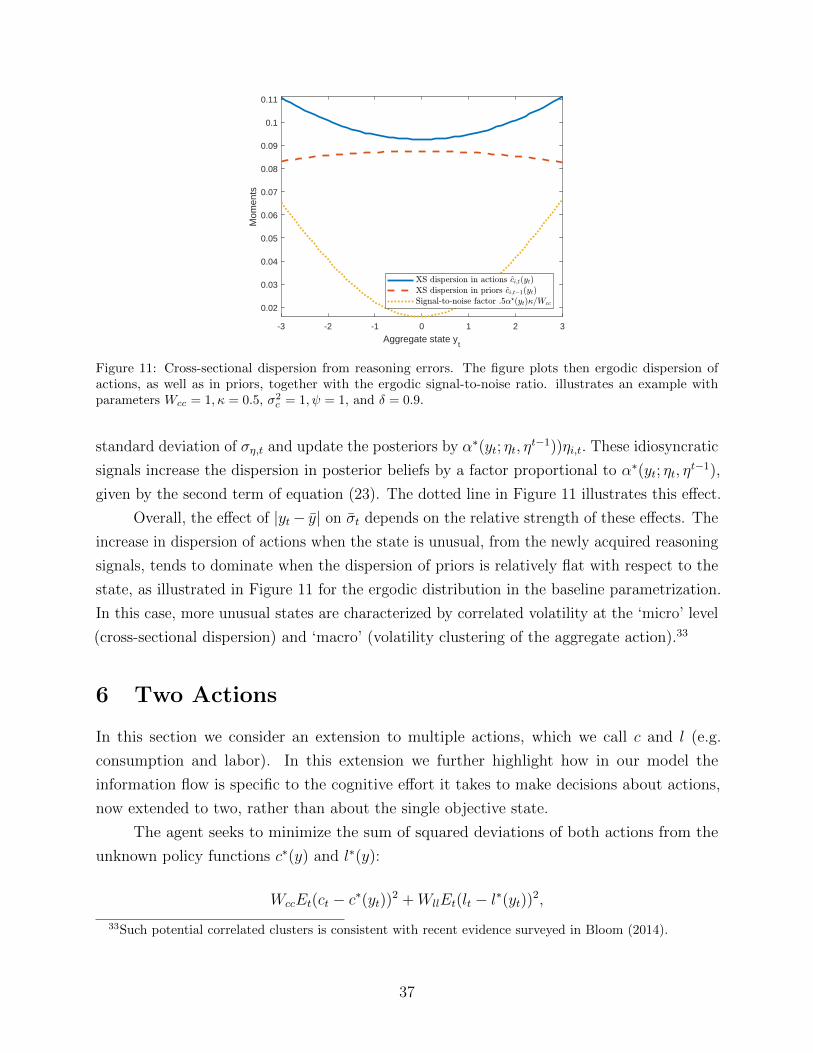
-3 -2 -1 0 1 2 3
Aggregate state yt
0.02
0.03
0.04
0.05
0.06
0.07
0.08
0.09
0.1
0.11
Mom
ents
Figure 11: Cross-sectional dispersion from reasoning errors. The figure plots then ergodic dispersion ofactions, as well as in priors, together with the ergodic signal-to-noise ratio. illustrates an example withparameters Wcc = 1, κ = 0.5, σ2
c = 1, ψ = 1, and δ = 0.9.
standard deviation of ση,t and update the posteriors by α∗(yt; ηt, ηt−1))ηi,t. These idiosyncratic
signals increase the dispersion in posterior beliefs by a factor proportional to α∗(yt; ηt, ηt−1),
given by the second term of equation (23). The dotted line in Figure 11 illustrates this effect.
Overall, the effect of |yt− y| on σt depends on the relative strength of these effects. The
increase in dispersion of actions when the state is unusual, from the newly acquired reasoning
signals, tends to dominate when the dispersion of priors is relatively flat with respect to the
state, as illustrated in Figure 11 for the ergodic distribution in the baseline parametrization.
In this case, more unusual states are characterized by correlated volatility at the ‘micro’ level
(cross-sectional dispersion) and ‘macro’ (volatility clustering of the aggregate action).33
6 Two Actions
In this section we consider an extension to multiple actions, which we call c and l (e.g.
consumption and labor). In this extension we further highlight how in our model the
information flow is specific to the cognitive effort it takes to make decisions about actions,
now extended to two, rather than about the single objective state.
The agent seeks to minimize the sum of squared deviations of both actions from the
unknown policy functions c∗(y) and l∗(y):
WccEt(ct − c∗(yt))2 +WllEt(lt − l∗(yt))2,33Such potential correlated clusters is consistent with recent evidence surveyed in Bloom (2014).
37

where Wcc and Wll are the costs of making the respective errors. We use a similar approach
as for the single action to model learning about the vector of functions [c∗(y), l∗(y)] as a
vector Gaussian Process distribution. The cognition cost is again a linear function of the
total information acquired about the vector, as measured by Shannon mutual information.
In Appendix D we present details on the setup and updating formulas. The optimal
precision of the deliberation signals about the two functions is to target, similarly to equation
(8) but this time potentially action specific, an optimal level for the posterior uncertainty
σ∗2c,t(yt) =κ
2Wcc
; σ∗2l,t(yt) =κ
2Wll
, (24)
where κ is the marginal cost of acquired information. The optimal signal-to-noise ratios and
the resulting actions ct(yt), lt(yt) are the counterpart of equations (11) and (10), respectively.
The basic features of the ergodic distribution of beliefs are thus similar to the univariate
case. The most interesting new implications of the multidimensional problem presented here
arise when there is an asymmetry in the costliness of mistakes. We assume that Wcc > Wll
and illustrate the ergodic effective policy functions of such an example in Figure 12.
0.5 0.6 0.7 0.8 0.9 1 1.1 1.2 1.3 1.4 1.5
y
0.5
0.6
0.7
0.8
0.9
1
1.1
1.2
1.3
1.4
1.5
Act
ion
(a) effective c policy
0.5 0.6 0.7 0.8 0.9 1 1.1 1.2 1.3 1.4 1.5
y
0.5
0.6
0.7
0.8
0.9
1
1.1
1.2
1.3
1.4
1.5
Act
ion
(b) effective l policy
Figure 12: Two Actions Optimal Policy. Benchmark values – Wcc = 1,Wll = 0.5, κ = 0.5, σ2c = 1, σ2
l =1, σ2
cl = 0, ψ = 1, and δ = 0.9. Changing values: κ = 0.15, ψ = 3, and δ = 0.99.
Both policy functions display the non-linearity of the univariate case, with a region of
relative inertia around y, and salience-like effects for more distant values. However, there are
differences in how the two effective policy functions, c and l, display those basic non-linear
features. Since the cost of mistakes is lower for the second action the agent optimally
deliberates less about it. At the ergodic distribution, this results in a function l that is much
flatter than c, and that also displays less reaction even in the tails of yt realizations.
38

The differential non-linearity across the two effective actions has implications for the
correlations in the errors made in the two actions. If the friction was in observing the objective
state yt, the resulting errors in the two actions would be perfectly correlated. In that case,
any information about the unknown yt informs both actions equally because the agent has
full knowledge of the two (linear) optimal policy functions. As a result, errors in both are
due to perceptions in the state yt, and are thus perfectly correlated. To the contrary, in our
model the errors are action specific. Moreover, because of the ergodic distribution of beliefs,
the errors will be more correlated for yt closer to y, where the agent relies more on the ergodic
prior beliefs (which are increasing for both actions). And the errors in the two actions will
be less correlated for unusual realizations of yt, where the agent leans more heavily on the
new reasoning signals, which feature uncorrelated error terms. For example, to an outside
observed this could look like a shift in preferences.
Our setup also affects inference about the size of the underlying cognitive friction.
Consider an analyst that looks at our data through the lenses of a model of imperfect
perception of states but known policy functions. Suppose the analyst then estimates the
constant signal-to-noise ratio, corresponding to α∗y in equation (14), that best fits a linear
function through the observed ct action (dashed line in Figure 12). While the fitted response
cannot deliver the non-linear features of the optimal ct(y), it will at least imply behavior that
is on average correct with respect to that generated by our model.
However, if the analyst uses the estimated model to predict the agent’s behavior in
terms of the other action, the prediction will be biased on average, as illustrated in the right
panel of Figure 12. The predicted policy function lt is the same as that for ct, since they are
both driven by the same underlying belief about yt. When the analyst’s model sees data on
ct, which tracks the optimal c∗(y) better, it infers that the agent pays a lot of attention to
yt. With precise beliefs about yt, a model of imperfect perception of states implies that the
agent sets both actions accurately, resulting in a responsive lt. To the contrary, however, in
our model the agent generally does not respond much in lt, and in particular much less than
ct. Moreover, in our model changing the costliness of mistakes (e.g. Wcc) will affect only
the precision in the ct action. However, in the other model changing information about yt is
chosen based on the weighted average of the costliness of mistakes in terms of both ct and lt.
Thus, changing Wcc would increase the precision in both actions.
7 Conclusion
In this paper we have developed a tractable and parsimonious model to study costly cognition.
We have assumed that agents perfectly observe state variables, but have limited cognitive
39

resources that prevent them from computing their optimal policy function. We have shown
that the resulting actions are characterized by several empirically plausible features: (i)
endogenous persistence: even if the observed states are iid, there is persistence in the
agent’s beliefs about the conditional optimal course of action; (ii) non-linearity: typical
behavior exhibits inertia and ‘salience’ effects; (iii) stochasticity: the action is stochastic, even
conditioning on the perfectly observed objective state, as it is driven by random reasoning
signals; (iv) cross-sectional heterogeneity in policy functions: agents’ experiences may lead
to average biases and local changes that are non-monotonic; (v) endogenous persistence in
the volatility of actions: following unusual times both the time-series and the cross-sectional
variance increases; (vi) state-dependent accuracy in different actions.
The model has potentially important policy implications. First, it offers a cohesive
framework to understand an array of features for the individual behavior. The errors made by
these agents do not arise from mechanical decision rules, but instead respond to the state and
the characteristics of the environment, including policy changes, in the spirit of Lucas (1976).
Second, the friction may help understand macroeconomic phenomena such as non-linearity,
persistence, volatility clustering, and in the process may change inference on the underlying
sources of economic mechanisms and shocks. Indeed, an econometrician that fits a standard
fully rational agent model to the equilibrium outcomes generated by our model may conclude
that there are policy-invariant sources of non-linearity and time-variation in parameters.
Instead, through the lenses of our model, these non-linearities and apparent time-varying
parameters are a manifestation of a single cognitive friction that leads economic agents to
act according to state-dependent reasoning rules.
Finally, our aggregate-level implications have abstracted from general equilibrium type
of interactions. Incorporating these interactions involves studying the propagation effects of
the state-dependent individual errors in actions, as well as modeling the agents’ reasoning
choice of computing potentially complex general equilibrium effects, issues that we find
promising for future research.
40

References
Akerlof, G. A. and J. L. Yellen (1985): “Can small deviations from rationalitymake significant differences to economic equilibria?” The American Economic Review, 75,708–720.
Alaoui, L. and A. Penta (2016): “Cost-Benefit Analysis in Reasoning,” Working Paper.
Angeletos, G.-M. and C. Lian (2017): “Dampening General Equilibrium: From Microto Macro,” NBER Working Paper No. 23379.
Aragones, E., I. Gilboa, A. Postlewaite, and D. Schmeidler (2005): “Fact-FreeLearning,” The American Economic Review, 95, pp–1355.
Ballinger, T. P. and N. T. Wilcox (1997): “Decisions, error and heterogeneity,” TheEconomic Journal, 107, 1090–1105.
Bishop, C. M. (2006): Pattern recognition and machine learning, Springer.
Bloom, N. (2014): “Fluctuations in Uncertainty,” Journal of Economic Perspectives, 28,153–176.
Caplin, A., M. Dean, and J. Leahy (2016): “Rational Inattention, Optimal ConsiderationSets and Stochastic choice,” Working paper.
Caplin, A., M. Dean, and D. Martin (2011): “Search and satisficing,” The AmericanEconomic Review, 101, 2899–2922.
Carvalho, L. and D. Silverman (2017): “Complexity and Sophistication,” WorkingPaper.
Christiano, L. J., M. Eichenbaum, and C. L. Evans (2005): “Nominal rigidities andthe dynamic effects of a shock to monetary policy,” Journal of political Economy, 113,1–45.
Cogley, T. and T. J. Sargent (2005): “Drifts and volatilities: monetary policies andoutcomes in the post WWII US,” Review of Economic Dynamics, 8, 262–302.
Deck, C. and S. Jahedi (2015): “The effect of cognitive load on economic decision making:A survey and new experiments,” European Economic Review, 78, 97–119.
Dupor, B. (2005): “Stabilizing non-fundamental asset price movements under discretionand limited information,” Journal of Monetary Economics, 52, 727–747.
Ergin, H. and T. Sarver (2010): “A unique costly contemplation representation,” Econo-metrica, 78, 1285–1339.
Evans, G. W. and S. Honkapohja (2011): Learning and Expectations in Macroeconomics,Princeton University Press.
41
Farhi, E. and I. Werning (2017): “Monetary Policy, Bounded Rationality, and IncompleteMarkets,” NBER Working Paper No. 23281.
Fernandez-Villaverde, J., J. F. Rubio-Ramırez, and F. Schorfheide (2016):“Solution and estimation methods for DSGE models,” Handbook of Macroeconomics, 2,527–724.
Gabaix, X. (2014): “A sparsity-based model of bounded rationality,” The Quarterly Journalof Economics, 129, 1661–1710.
——— (2016): “Behavioral macroeconomics via sparse dynamic programming,” NBERWorking Paper 21848.
Garcıa-Schmidt, M. and M. Woodford (2015): “Are low interest rates deflationary?A paradox of perfect-foresight analysis,” NBER Working Paper No. 21614.
Hassan, T. A. and T. M. Mertens (2017): “The social cost of near-rational investment,”The American Economic Review, 107, 1059–1103.
Hey, J. D. (2001): “Does repetition improve consistency?” Experimental Economics, 4,5–54.
Ilut, C., R. Valchev, and N. Vincent (2016): “Paralyzed by Fear: Rigid and DiscretePricing under Demand Uncertainty,” NBER Working Paper 22490.
Justiniano, A. and G. E. Primiceri (2008): “The time-varying volatility of macroeco-nomic fluctuations,” The American Economic Review, 98, 604–641.
Kacperczyk, M., S. van Nieuwerburgh, and L. Veldkamp (2016): “A rationaltheory of mutual funds’ attention allocation,” Econometrica, 84, 571–626.
Kalaycı, K. and M. Serra-Garcia (2016): “Complexity and biases,” ExperimentalEconomics, 19, 31–50.
Liu, W., J. C. Principe, and S. Haykin (2011): Kernel adaptive filtering: a comprehensiveintroduction, vol. 57, John Wiley & Sons.
Lucas, R. E. (1976): “Econometric policy evaluation: A critique,” in Carnegie-Rochesterconference series on public policy, vol. 1, 19–46.
Luo, Y. (2008): “Consumption dynamics under information processing constraints,” Reviewof Economic Dynamics, 11, 366–385.
Mackowiak, B. and M. Wiederholt (2009): “Optimal sticky prices under rationalinattention,” The American Economic Review, 99, 769–803.
——— (2015a): “Business cycle dynamics under rational inattention,” The Review ofEconomic Studies, 82, 1502–1532.
——— (2015b): “Inattention to rare events,” Working Paper.
42
Matejka, F. (2015): “Rationally inattentive seller: Sales and discrete pricing,” The Reviewof Economic Studies, 83, 1125–1155.
Matejka, F. and A. McKay (2014): “Rational inattention to discrete choices: A newfoundation for the multinomial logit model,” The American Economic Review, 105, 272–298.
Matejka, F., J. Steiner, and C. Stewart (2017): “Rational Inattention Dynamics:Inertia and Delay in Decision-Making,” Econometrica, 85, 521–553.
Mattsson, L.-G. and J. W. Weibull (2002): “Probabilistic choice and procedurallybounded rationality,” Games and Economic Behavior, 41, 61–78.
Melosi, L. (2014): “Estimating models with dispersed information,” American EconomicJournal: Macroeconomics, 6, 1–31.
Mosteller, F. and P. Nogee (1951): “An experimental measurement of utility,” Journalof Political Economy, 59, 371–404.
Nimark, K. (2014): “Man-bites-dog business cycles,” The American Economic Review, 104,2320–2367.
Nimark, K. P. and S. Pitschner (2017): “News Media and Delegated InformationChoice,” Working Paper.
Oliveira, H., T. Denti, M. Mihm, and K. Ozbek (2017): “Rationally inattentivepreferences and hidden information costs,” Theoretical Economics, 12, 621–654.
Paciello, L. and M. Wiederholt (2013): “Exogenous Information, Endogenous Infor-mation, and Optimal Monetary Policy,” Review of Economic Studies, 81, 356–388.
Rasmussen, C. E. and C. K. Williams (2006): Gaussian processes for machine learning,vol. 1, MIT press Cambridge.
Reis, R. (2006a): “Inattentive consumers,” Journal of Monetary Economics, 53, 1761–1800.
——— (2006b): “Inattentive producers,” The Review of Economic Studies, 73, 793–821.
Samuelson, W. and R. Zeckhauser (1988): “Status quo bias in decision making,”Journal of risk and uncertainty, 1, 7–59.
Sargent, T. J. (1993): Bounded Rationality in Macroeconomics, Oxford University Press.
Simon, H. A. (1955): “A behavioral model of rational choice,” The Quarterly Journal ofEconomics, 69, 99–118.
——— (1976): “From substantive to procedural rationality,” in 25 years of economic theory,Springer, 65–86.
Sims, C. A. (1998): “Stickiness,” in Carnegie-Rochester Conference Series on Public Policy,vol. 49, 317–356.
43

——— (2003): “Implications of rational inattention,” Journal of Monetary Economics, 50,665–690.
——— (2006): “Rational inattention: Beyond the linear-quadratic case,” The Americaneconomic review, 96, 158–163.
——— (2010): “Rational inattention and monetary economics,” in Handbook of MonetaryEconomics, ed. by B. M. Friedman and M. Woodford, Elsevier, vol. 3, 155–181.
Smets, F. and R. Wouters (2007): “Shocks and frictions in US business cycles: ABayesian DSGE approach,” The American Economic Review, 97, 586–606.
Stevens, L. (2014): “Coarse Pricing Policies,” Manuscript, Univ. of Maryland.
Stock, J. H. and M. W. Watson (2002): “Has the US business cycle changed and why?”NBER Macroeconomics Annual, 17, 159–218.
Tutino, A. (2013): “Rationally inattentive consumption choices,” Review of EconomicDynamics, 16, 421–439.
Tversky, A. and D. Kahneman (1975): “Judgment under uncertainty: Heuristics andBiases,” in Utility, probability, and human decision making, 141–162.
Valchev, R. (2017): “Dynamic Information Acquisition and Portfolio Bias,” Boston CollegeWorking Paper.
Van Damme, E. (1987): Stability and perfection of Nash equilibria, Springer Verlag.
van Nieuwerburgh, S. and L. Veldkamp (2009): “Information immobility and thehome bias puzzle,” The Journal of Finance, 64, 1187–1215.
——— (2010): “Information acquisition and under-diversification,” The Review of EconomicStudies, 77, 779–805.
Veldkamp, L. L. (2011): Information choice in macroeconomics and finance, PrincetonUniversity Press.
Wiederholt, M. (2010): “Rational Inattention,” in The New Palgrave Dictionary ofEconomics, ed. by S. N. Durlauf and L. E. Blume, Palgrave Macmillan, vol. 4.
Woodford, M. (2003): “Imperfect Common Knowledge and the Effects of MonetaryPolicy,” Knowledge, Information, and Expectations in Modern Macroeconomics: In Honorof Edmund S. Phelps, 25.
——— (2009): “Information-constrained state-dependent pricing,” Journal of MonetaryEconomics, 56, S100–S124.
——— (2014): “Stochastic choice: An optimizing neuroeconomic model,” The AmericanEconomic Review, 104, 495–500.
44

A Additional figures for section 4
In this Appendix we discuss in more detail how information propagates in the case of atime-zero prior mean that is steeper than the truth, i.e. a b0 > 1 in equation (18). Recallthat the right panel of Figure 7 plots the mean ergodic policy function in such a case.
Consider the impulse response experiment discussed in section 4.1.1 and plotted inFigure 13. In the left panel we see how on impact the action drops by more than the changein the state because the ergodic policy is now steeper. On the other hand, the innovation inthe new signal, ηt − css0 (yt), is now positive on average which updates upwards the beliefsabout c∗(y). As a result, the impulse response converges from above. The learning parametershave the usual effect as in the benchmark case: the response on impact is closer to the trueoptimal policy function and there is less propagation of the innovation for a lower κ and ahigher ψ. Without discounting, there are no persistent effects. In the right panel, we see thatwhen the true innovation is even more unusual the action further drops, but proportionallyless. The reason for this diminished impact effect is that the ergodic policy function becomesnow flatter as the state becomes more unusual. However, the reasoning precision is notaffected by the prior mean so the agent still obtains a more precise signal at the unusualstate. Therefore, in terms of propagation, the response conditional on a more unusual stateis still more persistent as in the benchmark case.
2 4 6 8 10 12 14 16 18
time
-50
-45
-40
-35
-30
-25
-20
-15
-10
-5
0
Per
cent
dev
iatio
n fr
om m
ean
(a) Alternative parameterizations
5 10 15 20 25 30 35 40
time
-60
-50
-40
-30
-20
-10
0
10
Per
cent
dev
iatio
n fr
om m
ean
(b) Alternative shock realizations
Figure 13: Impulse response function. The figure plots the typical path of the action when the time-zeroprior mean is steeper than the truth, i.e. c0(y) = c+ b0(y − y) with b0 = 3. The left panel plots the responsefollowing an innovation of yt = y − 2σy. The figure illustrates an example with parameters Wcc = 1, κ = 0.5,σ2c = 1, ψ = 1, and δ = 0.9. In the left panel we change parameters to κ = 0.1, ψ = 5 and δ = 1, respectively.
In the right panel we change persistence to ρy = .9 (dashed line), or we feed in future values of yt+j thatalways equal to y (starred line), or set the current shock to yt = y − 3σy (dotted line).
Figure 14 plots the experiments analyzed in section 4.2 in the case of b0 = 3. Thestate-dependent reasoning choice leads to more informative signals following periods of moreunusual states. Since in this case, the ergodic mean prior is steeper than the truth, the newsignals lead to updated beliefs characterized by flatter responses to y. We see this effect in
45
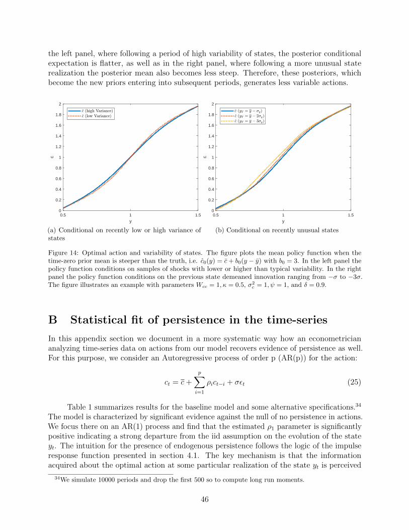
the left panel, where following a period of high variability of states, the posterior conditionalexpectation is flatter, as well as in the right panel, where following a more unusual staterealization the posterior mean also becomes less steep. Therefore, these posteriors, whichbecome the new priors entering into subsequent periods, generates less variable actions.
0.5 1 1.5
y
0
0.2
0.4
0.6
0.8
1
1.2
1.4
1.6
1.8
2
c
(a) Conditional on recently low or high variance ofstates
0.5 1 1.5
y
0
0.2
0.4
0.6
0.8
1
1.2
1.4
1.6
1.8
2
c
(b) Conditional on recently unusual states
Figure 14: Optimal action and variability of states. The figure plots the mean policy function when thetime-zero prior mean is steeper than the truth, i.e. c0(y) = c+ b0(y − y) with b0 = 3. In the left panel thepolicy function conditions on samples of shocks with lower or higher than typical variability. In the rightpanel the policy function conditions on the previous state demeaned innovation ranging from −σ to −3σ.The figure illustrates an example with parameters Wcc = 1, κ = 0.5, σ2
c = 1, ψ = 1, and δ = 0.9.
B Statistical fit of persistence in the time-series
In this appendix section we document in a more systematic way how an econometriciananalyzing time-series data on actions from our model recovers evidence of persistence as well.For this purpose, we consider an Autoregressive process of order p (AR(p)) for the action:
ct = c+
p∑i=1
ρict−i + σεt (25)
Table 1 summarizes results for the baseline model and some alternative specifications.34
The model is characterized by significant evidence against the null of no persistence in actions.We focus there on an AR(1) process and find that the estimated ρ1 parameter is significantlypositive indicating a strong departure from the iid assumption on the evolution of the stateyt. The intuition for the presence of endogenous persistence follows the logic of the impulseresponse function presented in section 4.1. The key mechanism is that the informationacquired about the optimal action at some particular realization of the state yt is perceived
34We simulate 10000 periods and drop the first 500 so to compute long run moments.
46

Table 1: Time-series properties of the action
Moment \Model Baseline Lower κ Higher ψ
Persistence ρ1 .61 .18 .19
[.59,.63] [.17,.21] [.17,.21]
Note: This table reports results for estimating ρ1 in equation (25).The baseline parametrization is Wcc =
1, κ = 0.5, σ2c = 1, ψ = 1, and δ = 0.9. In the third column κ = .1, while in the fourth column ψ = 5. In
squared brackets we report the 95% confidence interval.
to be informative about the optimal action at a different value y′. The discussion in sections3.3 and 4.1 highlights the two essential structural forces for these time-series results. InTable 1 both for the alternative parameterizations of ’Lower κ’ and ’Higher ψ’, the effects ofreasoning about the optimal function are weaker, in the form of smaller estimated ρ1.
In Table 2, we also estimate an AR(2) process and the best fitting AR(p) model. Forthe baseline parametrization the AR(2) improves the fit over the AR(1) with significantcoefficients at both lags. The best fit, according to the Akaike information criterion, has 6lags with a sum of coefficients equal to 0.71. While in the baseline model the state is iid, weexplore the effects of increasing that persistence to 0.5 and 0.9, respectively. In the formercase, the cognition friction leads to a higher persistence in actions, equal to 0.83. In the lattercase, the model also generates significant hump-shape dynamics. In particular, when we fitan AR(2) process, the impulse response function transmits a raise in ct into an increase inct+j that mean reverts only at j = 6. This confirms the hump-shape dynamics in Figure 8.
Table 2: AR(p) processes for action
Model/Moment AR(1) AR(2) AR(p)
Persistence in actions ρ ρ1 ρ2 p∗p∗∑i=1
ρi
Baseline .61 .48 .2 6 .71
Shock persistence ρy = .5 .83 .85 -.02 5 .83
Shock persistence ρy = .9 .97 1.15 -.18 8 .95
Note: This table reports results for estimating AR(p) processes for the average action, as in equation (25). .
C Statistical fit of volatility clustering in the time-series
To measure volatility clustering, we first use the AR(p) regression in equation (25) tocompute squared residuals ε2t . We then regress them on the previous absolute value of actions
47

ct−1 ≡ ct−1I(|ct−1| > σ), where the latter indicator equals one if the absolute value of theaction ct−1 is larger than a threshold proportional to the measured unconditional standarddeviation of actions, denoted by σ. The regression states:
ε2t = α + β|ct−1|+ εt (26)
Table 3: Time-series properties of the action
Moment \Model Baseline Lower κ Higher ψ
Volatility cluster β .6 .48 .5
[.3,1] [-.01,1] [0,1]
Note: This table reports results for estimating β in equation (26) for the baseline and alternative parametriza-
tions of Table 1. In squared brackets we report the 95% confidence interval.
Table 3 reports evidence for volatility clustering, in the form of a significantly positiveβ in equation (26).35 The intuition for this finding is presented in section 4.2.1. After moreunusual states, which in turn generate more unusual actions compared to the ergodic action,in the form of a higher |ct−1|, the agent finds it optimal to reason more intensely. Thisincreased deliberation leads on average to an updated belief that is more responsive, whichon average generates a larger variability in actions in the next period, resulting in largerresiduals ε2t . The effects are smaller for the ’Lower κ’ and ’Higher ψ’ cases.
D Two Actions
In this appendix we present details on the extension to multiple actions introduced in section6. We model uncertainty over the vector of functions [c∗(y), l∗(y)] as a vector GaussianProcess distribution,[
c∗(y)l∗(y)
]∼ GP
([c0(y)
l0(y)
],
[Σc
0(y, y′) Σcl
0 (y, y′)Σcl
0 (y, y′) Σl0(y, y
′)
]),
where now c0(y) and l0(y) represent the prior mean functions over c∗(y) and l∗(y), respectively,and Σc
0(y, y′) and Σl
0(y, y′) are the covariances within the two functions c∗(y) and l∗(y)
respectively, and Σcl0 (y, y′) is the covariance across the two functions. All covariance functions
are of the squared exponential family
Cov(c∗(y), c∗(y′)) = σ2ce−ψc(y−y′)2 ; Cov(l∗(y), l∗(y′)) = σ2
l e−ψl(y−y′)2
35If instead of the threshold σ in the indicator function in (26), we use a value of 0, then the point estimatefor β is still positive but not significant at a 95% confidence level.
48

including the cross-term Cov(c∗(y), l∗(y′)) = σ2cle−ψcl(y−y′)2 , where the respective parameters
play the same role as before. We focus on the case where ψc = ψl = ψcl = ψ.The deliberation process is modeled as a choice over the precision of unbiased signals
ηct = c∗(yt) + εηct ; ηlt = l∗(yt) + εηlt
Lastly, the cognition cost is again a linear function of the total information the agent acquiresabout his (vector of) optimal actions, as measured by Shannon mutual information:
I(
[c∗(y)l∗(y)
];η(yt),η
t−1) = H(
[c∗(y)l∗(y)
]|ηt−1)−H(
[c∗(y)l∗(y)
]|ηt,ηt−1)
where we define the bold symbol ηt as the vector of signals ηct , ηlt.
Hence the costly deliberation framework is an extension of the univariate case. Theagent faces the following reasoning problem:
U = maxσ2c,t,σ
2l,t
−Wccσ2c,t(yt)−Wllσ
2l,t(yt)− κI(
[c∗(y)l∗(y)
];ηt,η
t−1)
s.t. σ2c,t(yt) ≤ σ2
c,t−1(yt); σ2l,t(yt) ≤ σ2
l,t−1(yt)
where for convenience we define the notation
σ2c,t(yt) = Vart(c
∗(yt)); σ2l,t(yt) = Vart(l
∗(yt))
Given an optimal choice of the signal error variance, there are corresponding effectivesignal to noise ratios α∗c(yt;ηt,η
t−1) and α∗l (yt;ηt;ηt−1) respectively, and the resulting effective
actions taken by the agent are given by:
ct(yt) = Et(c∗(yt)) = ct−1(yt) + α∗c(yt;ηt,η
t−1)(ηct − ct−1(yt))
lt(yt) = Et(l∗(yt)) = lt−1(yt) + α∗l (yt;ηt,η
t−1)(ηlt − lt−1(yt))
We focus on the case where the agent has a prior belief that there is no correlationbetween the values of his two actions and hence σ2
cl = 0.36 The optimal deliberation choice isrepresented by, this time potentially action specific, optimal target levels for the posterioruncertainty, which lead to the equation (24) in the text
σ∗2c,t(yt) = min{ κ
2Wcc
, σc,t−1(yt)}; σ∗2l,t(yt) = min{ κ
2Wll
, σl,t−1(yt)}
36This is a particularly straightforward case to analyze because the optimal deliberation about each actionis independent of the choice of deliberation about the other. Moreover, it is still an interesting special casebecause some of the fundamental features of the more general problem are quite transparent here.
49