economia e statistica agroalimentare - …amsdottorato.unibo.it/6005/1/piras_francesco_tesi.pdfa new...
TRANSCRIPT

AAllmmaa MMaatteerr SSttuuddiioorruumm –– UUnniivveerrssiittàà ddii BBoollooggnnaa
DOTTORATO DI RICERCA IN
ECONOMIA E STATISTICA AGROALIMENTARE
Ciclo XXV
A NEW GLOBAL WHEAT MARKET MODEL
(GLOWMM) FOR THE ANALYSIS OF WHEAT
EXPORT PRICES
Settore Concorsuale di afferenza: 13/A4 - Economia Applicata
Settore Scientifico disciplinare:SECS-P/06 - Economia Applicata
Presentata da: Dott. Francesco Piras
Coordinatore Dottorato Relatore
Prof. Roberto Fanfani Prof. Luciano Gutierrez
Esame finale anno 2013

To my parents

ACKNOWLEDGMENTS
This thesis wouldn’t have been possible without the support and the friendship of some
people who introduced me in the research world.
I am most grateful to Luciano Gutierrez; Department of Agriculture, University of
Sassari; for having assisted me during this three years providing continuous suggestions
and advices.
Working with Luciano has been an extraordinary opportunity under human and scientific
point of view.
My acknowledgments also go to Sophia Davidova; School of Economics, University of
Kent; for the amazing period spent in Canterbury within the School of Economics.
In preparing this thesis I have also benefited greatly from comments and suggestions by
seminar participants at AIEEA Conference in Parma.
An finally, I would like to thank my family for their support.


INDEX INTRODUCTION ............................................................................................................................................. 1
1. LITERATURE REVIEW ...................................................................................................................................... 8
1.1 Increases in the price of crude oil .......................................................................................................... 21
1.1.1 Biodiesel .......................................................................................................................................... 23
1.1.2 Ethanol ............................................................................................................................................ 24
1.2 Exchange rates and us dollar depreciation ............................................................................................ 26
1.3 Speculative and investor activity ........................................................................................................... 28
1.3.1 Excess liquidity and index funds activity ......................................................................................... 28
1.3.2 Speculation ...................................................................................................................................... 29
1.3.3 Actors involved................................................................................................................................ 30
1.3.4 Place of transaction......................................................................................................................... 31
1.3.5 Speculative influence on commodity futures price ........................................................................ 33
1.4 Decline of commodity stocks ................................................................................................................. 40
2. THE STORAGE MODEL .................................................................................................................................. 44
2.1 Introduction ........................................................................................................................................... 44
2.2 Outline of the basic model ..................................................................................................................... 46
2.2.1 The weather and yields ................................................................................................................... 46
2.2.2 The groups included ........................................................................................................................ 46
2.2.3 The nature of storage...................................................................................................................... 47
2.2.4 The system ...................................................................................................................................... 48
2.3 The basic model ..................................................................................................................................... 48
2.3.1 Storers’ arbitrage relationships ...................................................................................................... 49
2.3.2 Market level price and quantities ................................................................................................... 51
2.4 The competitive profit-maximising storage rule ................................................................................... 53
2.5 The effects of storage on planned production ...................................................................................... 58
2.6 The effects of storage on market demand ............................................................................................ 60
2.7 Sequential equilibria in the system ........................................................................................................ 62
2.8 Challenging the basic storage model ..................................................................................................... 69
3. INTERNATIONAL WHEAT MARKET: A THEORETICAL FRAMEWORK ............................................................. 72
3.1 Price formation in world wheat market. A theoretical review .................................................................. 72
3.2 USDA wheat price determination model ................................................................................................... 77

3.2.1 Supply and demand factors affecting wheat price ..........................................................................77
3.2.2 Agricultural policies affecting wheat price ......................................................................................79
3.2.3 The pricing model ............................................................................................................................80
4. WORLD WHEAT MARKET IN TERMS OF PRODUCTION, CONSUMPTION AND TRADE .................................85
4.1 World wheat harvest Area .....................................................................................................................86
4.2 World wheat Yields.................................................................................................................................87
4.3 World wheat production ........................................................................................................................88
4.4 World wheat utilization ..........................................................................................................................90
4.4.1 World wheat food, seed and industrial use ....................................................................................92
4.5 World wheat export ...............................................................................................................................94
4.6 World wheat imports. ............................................................................................................................97
4.7 World wheat Ending stocks and world wheat ending stock-to-use .......................................................98
5. GLOBAL VECTOR AUTOREGRESSIVE MODEL (G_VAR) ...............................................................................102
5.1 A global model for the analysis of the wheat world market ................................................................103
5.2 The solution of the GVAR model ..........................................................................................................106
5.3 The dataset and empirical results ........................................................................................................108
5.4 Impulse Response Analysis ...................................................................................................................114
6. Concluding Remarks ...................................................................................................................................125
APPENDIX A ....................................................................................................................................................130
APPENDIX B ....................................................................................................................................................136
BIBLIOGRAFY ..................................................................................................................................................137


1
INTRODUCTION
Cheap food has been considered as a normal condition for almost 30 years. After the price
peak registered during the 1970s crisis, real food prices constantly declined during the
1980s and 1990s reaching the lowest level in the beginning 2000s after the Asia financial
crisis. According to this trend many countries saw little convenience to invest in
agricultural production considering food imports as a safe and efficient means of
achieving national food security. However, as international food commodities prices have
increased abruptly since 2002 and especially since late 2006 all these perceptions quickly
collapsed. The IMF’s index of internationally traded food commodities price increased
130 percent from January 2002 to June 2008 and 56 percent from January 2007 to June
2008 (Mitchell, 2008). The FAO food price index reached its peach in June 2008
increasing 55 percent between June 2007 and June 2008. Rice prices doubled within just
five months of 2008, from US$ 375/ton in January to $ 757/ton in June (Baffes and
Haniotis, 2010). The increase in food commodities prices was triggered off grains which
began a sharp increase in price in 2005. Maize price tripled from January 2005 until June
2008; wheat prices increased 127 percent and rice prices increased almost 170 percent
during the same period (Mitchell 2008). Furthermore, although food price are now lower
than the peck reached in 2008, real food price have been still significantly higher in 2009
and 2010 and a large number of institutions predict that real food prices will remain high
until at least the end of the next decade. The OECD and FAO outlook 2008-2017 expects
prices to come down again but not to their historical levels. In particular, over the coming
decade, prices in real terms of cereals, rice and oilseeds are estimates to be 10 percent to
35 percent higher than in the past decade.
There are a number of factors that have contributed to the rise in food price. The
identification of the main factors is still under debate. A large number of research studies
have attempted to identify the factors behind the prices crises but only a few have
attempted to define their relative importance by adding explicit orders of magnitude to
each factors. Obviously it is not an easy task to depict a clear picture of prices crisis
because it is a global phenomenon that involves a large number of distinct events. Much
of the non academic debate was not based on evidence derived from appropriate research.
On the other side, much academic research was also “quick and dirty” because the lack of

2
time and the need to provide a theoretical basis for the policy makers (Headey and Fan,
2010).
Despite this complexity, this piece of research presents a briefly review of existing
literature on food crises with the objective to analyze the nature of the recent boom in
food commodities by examining which key factors played a main role. According to the
most common literature, some explanations seem to be more reliable and rigorous than
others.
Unfavourable weather condition in major producing countries have been viewed as one
important factors according to OECD report (2008), Tangermann (2011) and OECD-FAO
(2011). Despite of this, Headey and Fan (2008) suggest that production shortfalls are a
normal occurrence in agricultural and low production in several countries were offset by
large crop in other regions. Macroeconomic conditions such as strong GDP growth and
subsequent stronger demand for food in some developing countries have also been
considered as a permanent factor behind the recent prices spike (see Von Braun, 2007;
Trosle, 2008; Carter et al., 2011; Krugman, 2011). Other studies have argued that low
level of real interest rates and growing money supply diverted investments away from
financial assets towards physical assets, including commodities. This excess of liquidity
in the global economy, with a depreciation of US dollar, resulted in inflation and in its
turn, in rising commodity prices and an increased commodities demand for importing
countries (see Calvo, 2008; Abbot et al. 2008; Mitchell, 2008; Timmer, 2009; Gilbert,
2010a; Tangermann 2011).
The excess of liquidity fostered financial investments in commodity future markets
convincing some authors that speculation and not fundamentals were behind the
commodities price boom and bust (Baffes and Haniotis, 2010; Masters, 2008; Soros
,2008; Calvo, 2008). Cooke and Robles (2009), Gilbert (2010b) and Gutierrez (2013)
found evidences that financial activities in future markets may be of use in explaining the
change in food price. However, a large strand of literature challenged the arguments
proposed by the bubble proponents through logical inconsistencies, conceptual errors and
empirical evidences showing that speculation did not have a significant role in rising
commodities food prices (see Krugman, 2009; Wolf, 2008; Wright, 2009; Irwin et al.,
2009; Sanders and Irwin, 2010; Baffes and Haniotis, 2010).

3
Other possible causes analysed in literature include the decline of commodity stocks, the
rising of crude oil price, biofuels production and finally panic buying, ban and export
restrictions.
The competitive storage model explains how commodity stocks can play a main role in
buffering price volatility (see the pioneering work of Gustafson 1958; but also Samuelson
1971; Wright and Williams 1982; Scheinkman and Schechtman 1983; Williams and
Wright 1991 and Deaton and Laroque 1992). Starting on the years 1999-2000, the global
stock level for major cereals has been declined reaching its historical low level in 2007
(Dawe, 2009; Wright, 2011; Tangermann, 2011). Therefore, it is not surprising that
literature has identified the reduction of commodity stocks as one of the main factors in
recent food price spike (Piesse and Thirtle, 2009; Trostle, 2008; Dawe, 2009). Empirical
evidence have been provided by Kim and Chavas (2002), Balcombe (2011), Carter et al.
(2011), Hochman et al. (2011), Serra and Gil (2012). Nevertheless, Dawe (2009) and
Roache (2010) remain less than convinced about the empirical importance of stock
depletion in food prices spike both in the short and long term.
The oil price represents a permanent factor in food price formation and some authors have
highlighted its possible importance as major factor in the recent prices boom (see Baffes,
2007; Baffes and Haniotis, 2010; Balcombe, 2011 among others). Moreover, as oil price
increases, biofuels becomes more competitive. Mitchell (2008), Baffes (2007), OCSE-
FAO (2011) and Tangermann (2011) suggest that biofuels contributed to the price crisis
in 2006-2008. Hochman et al. (2011) provide a complete literature about quantitative
estimates of biofuels impact on food commodity price index.
Finally, in response to rising food prices, some countries introduced protective policy
measures. Unfortunately, the final result of these measures is always a deeper prices
volatility and higher prices into global markets as described in Headey and Fan (2008),
Trostle (2008), OECD-FAO (2011) and Tangermann (2011).
Rising food prices mainly affects lower income consumers especially in poor countries
where households spend a great part of their income on food. This is particular true for
cereals and especially wheat. We focus on wheat market for two reasons. First, it
represents the most relevant source of food in developing countries. Second, this market
is deeply changed during the last decades evolving from an oligopoly between US and
Canada with the latter as a price leader (MaCalla, 1966) to a tripoly including also
Australia (Alouze et al. 1978) and hence to a price leadership model with US price leader

4
(Oleson 1979; Wilson, 1986). More recently, Westcott and Hoffman (1999) recognize
that, although US is the largest word wheat exporter, its market share is not enough to be
considered a price leader anymore. In essence wheat market is nowadays characterized by
a small number of wheat producing and exporting countries that sell to a relative large
group of importers, mostly developing countries.
While new market assumptions can be introduced for example in general equilibrium
models, more flexible models can be provided and used for the analysis of worldwide
commodity markets. The aim of the thesis is to model the impacts of the main factors
behind the wheat export price dynamics.
To this end, in this study we introduce a innovative worldwide dynamic model for the
analyses of short and long-run impulse responses of wheat commodity prices to various
real and financial shocks. Specifically, we propose a GLObal Wheat Market Model
(GLOWMM) to study the dynamic of wheat export prices.
The model is specified by using the Global Vector AutoRegressive (GVAR) model
proposed by Pesaran et al. (2004) and Dees et al. (2007). The methodology allows the
analysis of wheat export prices for the six main export countries, USA, Argentina,
Australia, Canada, Russia and EU.
The GVAR approach is particular appealing for the analysis of the worldwide wheat
market for two reasons. First, it is specifically designed to model fluctuations and
interactions between countries. This is a crucial asset given the features of world wheat
market and the global dimension of the food prices crisis that cannot be downsized to one
country, rather involves a large number of countries.
Secondly, the GVAR allows to model the dynamic of wheat export prices as results of the
effects exerted by the country-specific and by foreign-specific variables. The foreign-
specific variables are defined as weighted average of wheat export prices, the stock to
utilization ratio and the effective exchange rate fluctuations in all competitor countries.
Thus both country-specific as foreign-specific effects can be jointly modelled. For each
country model we hypothesize the weak exogeneity properties for both foreign-specific
and global variables. This accounts to assume the small economy hypothesis for each
country and, consequentially, that wheat export prices are determined in the worldwide
market.
Finally the GVAR model combines a number of atheoretic relationships. Unlike structural
models, as for example general equilibrium models, the approach does not attempt to

5
make restrictions, for example on the basis of economic theory. Causal relationships are
analyzed by means of the impulse response functions that, built from the GVAR
estimates, allow to highlight how shocks on wheat stocks and demand, exchange rates,
input prices or global oil price propagate at domestic and global level.
The research is organized into chapters. The first chapter is divided in five sections. The
first one presents a literature review of existing literature on food commodities prices
crisis. After that, the following sections consider some particular factors related to food
price increases that we think to be most important in explaining the price crisis. In fact,
the second major section focuses on the relationship between crude oil prices and
commodities prices. In the past, price of energy and agricultural commodities markets
have been studied by two distinct point of view. Today, it is clear how increasing oil price
can affect food prices both through the supply and demand side. Here we’ll focus on two
supply-side costs of agricultural production such as inputs and transport and one demand
side factors such as biofuels. A large strand of literature considers the price of crude oil
closely connected to the price of corn because of biofuels. In fact, as showed by Abbott et
all (2008), crude oil price determines the gasoline price which is in competition with the
ethanol price. As soon as the ethanol price become competitive with respect to the
gasoline price, the incentive to the ethanol capacity increases and this pushes up the corn
demand for ethanol industry and finally the corn price. In this section the relative
importance of subsidies and mandates in determining the corn price will be also
examined.
The third section deals with the exchange rate and particularly the US dollar depreciation.
This theme has been mentioned by a large strand of literature as a factor that might be
important in explaining the recent rising food prices. In this piece of research a
background on the economic forces that determine the low level of exchange rates in
2006-2008 will be provided. It will be also showed how commodities prices have
historically changed in function of the exchange rate. In essence we discuss the
relationship between exchange rate, commodities prices, inflation and international trade.
The fourth major section focuses on speculation in the commodity futures markets. A
large number of studies take into consideration the great amount of index funds
investments in the commodity markets in order to explain current commodities price
increase blaming speculators for a good part of this prices trend. However, different
authors consider the role of speculators as an important role in functioning of

6
commodities market as we will see. It will be analysed in more detail whether the
increased speculation activity, as sustained by a large strand of literature, is a driver for
increased price volatility and the overall level of commodity price.
The last section describes the roles of another key driver of agricultural markets and price
volatility, the stock level. Commodity storage clearly plays an important buffering role by
mitigating the gap between demand and supply level at least in short term and reducing
the price volatility (see OECD-FAO, 2011). In essence, when stocks level is low, supply
becomes very inelastic and even a small additional difference between demand and
supply can result in a huge price increases. Price crisis in cereal markets have often
occurred with a low stock to use ratios such as in 2006-2008 as noted by a large strand of
literature.
Considering the main role played by stocks level in agricultural market, the second
chapter presents the competitive storage model described by Williams and Wright (1991),
which views inventories as the main determinant in commodity price behaviour. In order
to explain commodity booms and busts, the model provide a deep understanding of what
determines stock levels and, in particular, what may cause inventories to be depleted.
The third chapter explores the price formation mechanisms of word wheat market
presenting different theoretical models discussed since the 60’s in order to provide a
theoretical framework for analysing wheat price behaviour. Particular attention will be
reserved on the recent annual model for the United States wheat price firm used by
USDA in short term market analysis and long term base line projection.
The fourth chapter is closely connected to the previous one providing a complete picture
of world wheat market in terms of production, consumption and trade using data covering
the last decades and focusing on the last three years. According to these data, it will be
clear how a few countries strongly influences global wheat market producing and
exporting a large portion of global wheat availability. Also the ending stocks of wheat in
global markets appears concentrated in few countries or regions. On the other hand, world
wheat import market is not so concentrated. In essence it will be seen how the global
wheat market is characterized by a small number of wheat exporting and producing
countries that sell to a relative larger group of importers. China and India represent a
particular case. They are two major wheat producing countries with a marginal role in
trade focusing mostly on domestic market.

7
Chapter five describes the empirical model used in this piece of research. For our research
it will be used a worldwide dynamic model that provides short and long-run impulse
responses of wheat prices to various real and exogenous shocks. We used the Global
Vector Autoregressive modelling approach with exogenous variables, to estimate a
Global Agrifood Vector AutoRegressive model. The methodology allows to model EU
and non-EU countries, and to aggregate the single regional VARX models into a global
model by using weighting matrices mainly based on the share of wheat international
market (measured in term of export) of each country involved in the research.
In essence the model provides a general and practical modelling framework for
quantitative analysis of the relative importance of different shocks on agro-food sectors.
Specifically, using this strategy we analyze channels of transmission from external
shocks that affect crops productivity and, in its turn, wheat prices. The dynamic properties
of the GVAR model will be investigated by means of the Generalized Impulse Response
Function (GIRF). In order to investigate how export prices are affected by some shocks
we assume a negative standard error shock that affect the main exogenous variables in all
export countries and simulate the effect on wheat export prices up to a limit of 24 months.
More in details, we analyze the implications of five different external shocks:
A one standard error negative shock to US stock to utilization ratio
A one standard error negative shock to global stock to utilization ratio
A one standard error positive shock to oil price
A one standard error negative shock to real effective exchange rate
A one standard error positive shock to fertilizer price
Impulse response analysis reveals that a decrease of wheat stocks with respect to the level
of consumption, increasing oil prices and real exchange rate devaluation have all
inflationary effects on wheat export prices although their impacts are different among the
main export countries.
Finally, the last chapter concludes.

8
1. LITERATURE REVIEW
Between 2002 and 2008 nominal prices of energy and metals increased by 230%, those of
food doubled. The IMF’s index of internationally traded food commodities price
increased by 130% from January 2002 to June 2008 and by 56% from January 2007 to
June 2008 (Mitchell, 2008). The FAO food price index reached its peach in June 2008
increasing 55% between June 2007 and June 2008. Figure 1.1 below shows the FAO
Food Index of monthly prices for food commodities that are the basis for human
consumption. Between 1980 and 2002 prices, measured in nominal dollars, had a slightly
downward trend although there were several peaks such as in 1980, 1988 and 1996. After
2001 prices began to rise slowly but constantly reaching in 2004 the same level that they
registered in the middle of 1980s. However in early 2006, commodity food prices began
to rise more quickly until 2008 reaching new historical high.
Figure 1.1: FAO Food Index, 2002-2004=100
Source: Fao Food Index in nominal price 1990.1 – 2013.3
The same upward trend is well represented by FAO international Commodity price cited
by Tangermann (2011) that shows monthly prices of selected agricultural products in
international trade between 2005 and 2010 (figure 1.2).
50.0
100.0
150.0
200.0
250.0
300.0
Food Price Index Cereals Price Index

9
Figure 1.2: Monthly prices of selected Agricultural products, 2005-2010, (US$ per ton).
Source: FAO International Commodity Prices cited by Tangermann (2011).
http://www.fao.org/es/esc/prices/PricesServlet.jsp?lang=en
The recent boom presents some similarities with the two previous commodities prices
crisis, the Korean war crisis and the 1970s energy crisis. According to Baffes and
Haniotis (2010) and also Vaciago (2008), each crisis happened during a period of high
and sustained economic growth and in an expansionary macroeconomic environment.
Moreover, all the crisis considered were followed by a severe slowdown of economic
activity. Despite of these aspects, the three crisis shows also some important differences.
The recent crisis has been the longest in term of time length and the broadest in term of
numbers of commodities involved. Baffes and Haniotis (2010) noted that the recent prices
boom has been the only one to involved all three main groups of commodities (energy,
metals and agricultural); it was not associated with high inflation unlike the other two
previous crisis and, finally, it ends with the simultaneously development of two other
crisis, in real estate and in equity markets whose end, in turns, led to the recent recession.
Figure 1.3 shows the price index for food commodities but also the index for the average
of all commodities and an index for crude oil in order to better understand how the recent
price crisis involved not only food commodities prices. As clearly described by Trostle
(2008), until 1999 all three index were at about the same level. From 1999 to March 2008
food commodities prices has risen almost 98% while the index for all commodities has
risen 286% during the same period and the index for crude oil has risen 547%. If
compared to these index, the recent uptrend of food commodities index might not seem so

10
huge after all. However, because rising food prices tend to negatively affect lower income
consumers more than other, food price boom is socially and politically sensitive.
Moreover, despite the price down trend after mid-2008, cereal prices increased again in
the second half of 2010 recalling back the negative memories of 2008 crises even if the
2010 situation differs from the 2008 price crises in some important aspects as well
described by Tangermann (2011).
Figure 1.3: Oil, all commodities and food commodities index.
Source: Trostle (2008:2) from International Monetary Fund: International Financial
statistics.
In the case of agricultural commodity prices spike, numerous proposal have been made
about which factors were the most important drivers in the 2006-2008 crisis. Commodity
prices were affected by a combination of factors including droughts in major grain
producing regions, low stocks of cereals and oilseeds, increased use of feedstock to
produce biofuels and rising crude oil price. Moreover, the depreciation of the US dollar is
also responsible since the price for the key commodities is typically quoted in US dollar.
A period of strong growth global economy and a large amount of liquidity also appears to
have contributed to a substantial increase in speculative interest in agricultural futures
markets (OECD, 2008b).

11
Headey and Fan (2008), suggested the hypothesis of the so called “perfect storm” based
on the interaction and conflagration of these factors. In fact, according to the authors it
should be considered the complex interactions between factors that reinforced each other
creating the condition for the perfect storm.
A few number of studies try to define the share of the prices increase that can be
attributed to each cause, but the larger part do not, rather indicating that the total effect on
prices derives from the combination of all these factors.
Moreover, policy response introduced by some countries in 2008 in order to offset the
rising food prices, such as export ban for the rice or prohibitive taxes, contributed to make
even worsen increasing the demand for commodities (Baffes and Haniotis, 2010; Sarris,
2009, Tangermann, 2011).
At the end of 2008 the weakening or reversal of these factors induced a quick prices fall
across most commodities sectors. The sharp declined was stressed by the simultaneously
financial crisis and the subsequent global economic downturn.
Although food prices are now lower than the peck reached in 2008, real food prices have
been still significantly higher in 2009 and 2010 and a large number of institutions predict
that real food prices will remain high until at least the end of the next decade. The OECD
and FAO outlook 2008-2017 expects, over the coming decade, prices in real terms of
cereals, rice and oilseeds to be 10% to 35% higher than in the past decade. According to
the European Commission prospects 2010-2020 (2010), commodity prices are expected
to stay firm over the medium term supported by factors such as the growth in global food
demand, the development of the biofuels sector and the long-term decline in food crop
productivity growth.
More in details, the medium-term prospects for the EU cereal markets depict a relatively
positive picture with tight market conditions, low stock levels and prices remaining above
long term averages. A similar picture is depicted for the medium-term prospects for the
EU oilseed markets characterized by strong demand and high oilseed oil prices.
In the next paragraphs will be reported some of the important studies summarizing the
major causes of food commodities prices boom.
The OECD Report (2008) divides factors behind the recent prices crisis between
transitory and permanent factors. The reduction of crop yields for some key agricultural
commodities due to unfavourable weather and water constrains in major producing
regions should be viewed as a temporary factor. In fact, unless permanent reduction in

12
yields, normal higher output can be expected in response to negative yield shocks. By the
way, the result of adverse weather in 2007 was a second consecutive drop in global
average yields for grains and oilseeds. Two sequential years of low global yields occurred
only three other times in the last 37 years according to Trostle (2008). As reported by
Tangermann (2011) cereals production in Australia, that is a wheat exporter country, was
affected by persistent drought in a row of years before 2008. In Canada, that is another
wheat exporter country, yields in 2006 and 2007 were substantially below the average
levels. Also in the EU, because unfavourable weather, cereals production fell by 8% from
2005 to 2007. Finally, Russia and Ukraine, two large exporter countries, were affected by
severe drought in 2007 and 2008. Moreover, this lower production forced the decline in
the global stocks and created a world market environment characterized by concern about
future availability of major commodities among importers. Despite of the low crop yields
between 2005 and 2007 demand for wheat and vegetable oil increased two percentage
points more than output (OCSE 2008b).
OCSE-FAO (2011) states that in 2010, adverse weather condition played an important
role in the commodity price spike registered also in that year. In particular drought
reduced the grain supply in the Russia Federation and Ukraine and flooding affected the
grain harvest in some important regions of Australia. Both these events shown their
impact on world commodity price volatility. The same OECD-FAO (2011) report
suggests that long term climate change will impact in a more adverse way tropical areas
than temperate areas. In particular Sub-Saharan Africa is expected to be the most
affected.
Despite of this, a closer inspection of the data suggests that this low level of production,
through attractive, is not convincing as it first appears in order to completely explain
rising food prices (OCSE-FAO, 2011). As suggested by Headey and Fan (2008) it should
be keep in mind that production shortfalls are a normal occurrence in agricultural
production and in wheat production in particular. Moreover low production in several
countries in 2007 were largely offset by large crop in Argentina, Kazakhstan, Russia and
United States.
Macroeconomic conditions such as strong GDP growth and subsequent stronger demand
for food in some developing countries should be considered as a permanent factor but not
as a new factor. It means that these change in macroeconomic conditions will be a
permanent factor in future price determination but have had no role in recent rising prices.

13
Trostle (2008) includes strong growth in demand in the long term factors that have
affected demand for commodities putting additional upward pressure on world prices.
The author identifies three factors at the basis of the strong growth in demand over the
last decade: the increasing population, the rapid economic growth especially in China and
India which account for 40% of the world’s population and the rising per capita meat
consumption. In essence, according to Trostle (2008:7) “as per capita income rose,
consumers in developing countries not only increased per capita consumption of staple
foods, they also diversified their diets to include more meat, dairy products and vegetable
oils, which in turn, amplified the demand for grains and oilseeds”. Cartel et al. (2011)
define China as a big force in the commodities prices spike. Its strong and increasing
demand of corn, wheat but also copper and oil pushed up commodities price during the
recent crises.
These aspects are confirmed by OECD-FAO (2011) that show how growing demand in
China and India has contributed to the decreasing of stocks and the increasing of prices.
However growing demand explanation in emerging economic is unconvincing for several
reasons. As suggested by OECD-FAO (2011) ,Tangermann (2011), Baffes and Haniotis
(2010), food demand in China and India had already grown rapidly before 2007.
Moreover, the price crises has been particularly pronounced in the cereals sector; a sector
where China and India are almost self sufficient.
Macro economic developments, in particular in the US, represented by low level of real
interest rates and growing money supply, diverted investments away from financial assets
towards physical assets, including commodities. This excess of liquidity in the global
economy, with a depreciation of US dollar, resulted in inflation and in its turn, in rising
commodity prices (see Calvo, 2008; Abbot et al. 2008; Mitchell, 2008; Timmer, 2009;
Gilbert, 2010a; Tangermann 2011).
Rapid economic growth in developing countries led to a rapid growth in the demand for
crude oil. For instance, Trostle (2008) states that the oil import of China alone increased
more than 21% per year from 194 million barrels in 1996 up to 1.37 billion barrels in
2006. This huge increase crude oil demand has contributed to a rapid rising oil price.
The oil price represent permanent factor in price food formation and is seen by OECD
(2008) and OCSE-FAO (2011) as major factor in the recent prices boom leading to higher
average prices level in the future. The long term link between energy, in particular oil
price, and food prices is stressed by Tungermann (2011). However, the same author

14
challenges the contribution of the energy price to the severe price spike of agricultural
commodities in 2006-08. This is because there should be, typically, one year lag in the
response of agricultural production to price signal. In essence, the spike in oil price
should not be simultaneously transmitted to commodity prices. Wright (2009) argued that
the prices of most fertilizers increased after and not before the cereals price boom.
The oil price spike is strongly correlated to biofuels production. As oil price increases,
biofules becomes more competitive. A large strand of literature (see for instance Mitchell,
2008; OCSE-FAO, 2011; Tangermann, 2011) considers highly likely that biofuels
contributed significantly to the price crisis in 2006-08 because an important part of
cereals and oilseeds production is used to increase biofuels supply and because land
substitution effect as it will be better explained.
Low inventory levels, expressed by the ratio stock to use, played an important role in the
2006-08 food commodity spike according to a large strand of literature (see Hochman,
2011, Tangermann, 2011, Wright, 2009). In 2007, stocks of wheat and vegetable oil have
reached their lowest levels relative to use reducing the buffer against shocks in supply and
demand. “When stocks are low, supply become very inelastic and even small additional
gaps between demand and supply can result in rather large price increase” (OECD-FAO,
2011). The reduction of stocks level is related not only to the gap between demand and
supply. An important role was played by political decisions of some important countries
such as China to reduce stocks. Stable food prices registered until 2002 allowed to adopt
the so called “just in time” inventory management based on buying commodities in the
world market instead to increase stocks holding. In addition, more liberalized trade
policies were largely adopted by a wide number of countries during the last decade
reducing the need for individual countries to hold high level of stocks. These new level of
low stocks are not expected to increase over the coming decade, hence representing a
permanent factor in price formation. Headey and Fan (2008) argue that stocks declines
are consistent with price boom but they should be consider a symptom of deeper causes
and not as one of the major factors behind rising prices. Furthermore, Dawe (2009) have
challenged the role of low stocks during the crisis arguing that the decline in global stocks
was due to a decrease in china’s stocks that are, historically, not used in stabilizing
international cereals market.
Finally, the recent wave of investment in futures commodity markets from non
traditional traders may have short term price effects. “Financial speculation which
15
involves trading in future markets and commodity derivatives without any link to the
underlying cash market has been suggested as one of the possible causes of volatile
agricultural commodity price movements” (OECD-FAO, 2011:64). This is particularly
true for investment bank, hedge fund, swap and other money managers whose role in
future commodity market greatly increased since the mid-2000s (Tungermann, 2011).
Moreover, given the size of funds recently involved in futures exchange markets, this new
factor is considered by OECD (2008) as a permanent element in future price volatility.
In response to rising food prices, some countries introduced protective policy measures in
order to reduce the impact of rising world food commodity prices on their own
consumers. Unfortunately, the final result of these measures is always a deeper prices
volatility and higher prices into global markets. This because world prices adjustments
had to be made by the smaller number of countries trading in the world that had not
introduced protective policies. We should distinguish between policies introduced by
exporting countries and polices introduced by importing countries. The formers have the
aim to discourage exports in order to keep domestic production within the country and so
keep the prices low. The most commonly used are the introduction of export taxes, export
quantitative restrictions, export bans, the elimination of export subsidies and so on. The
latter aim to reduce the impact of rising prices on consumers by reducing import costs and
hence providing lower prices to consumers. Import tariffs or subsidizes to consumers are
the most common import policies used by import countries during food prices crisis.
A detailed lists of policies responses to rising food prices introduced by some countries is
reported by Trostle (2008:23).
Headey and Fan (2008) discuss a series of commodity-specific factors that probably had a
role in increasing the price of some commodities. Government action and in particular
export ban or export restrictions, had a major role to the food price crisis during the 2006-
2008. This aspect is particularly true for rice market (OECD-FAO, 2011) where export
restrictions seems to be a major explanation because a large number of important
exporting countries had imposed export ban and also because only 7% of global rice
production is traded over the last five years making the rice market really thin. From
August 2005 until November 2007 rice prices increased constantly but significantly by
about 50% in real terms. In November 2007 India imposed the first major export ban.
From November 2007 to May 2008 rice price increased by 140% despite high level of
production patterns and the absence of any significant increase in demand. The rising rice

16
price continued until May 2008 when Japan withdrew its ban and realised 200,000 tons of
rice to Philippines. From then, prices fell almost immediately (Headey and Fan, 2008).
As well explained by OECD-FAO (2011), the timing of this export constraints was
important for the impact on the world market because the export restrictions limited the
traded volumes in the worst moment, when the price rise on international markets was
already accelerating. The final result was a greater uncertainty and a faster increase in
commodity prices.
This is in line with Tangermann (2011) that considers policy actions on export and import
side an important driver for the prices spike but much more important is considered the
effect of these policies in reinforcing the sentiment of excitement and panic in the market.
Tangermann (2011:30) provides also a complete and detailed list of policy measures
adopted in selected developing countries and in the major emerging economies in
response to the 2006-08 food crises analysing, for each kind of action, their impact and
outcome.
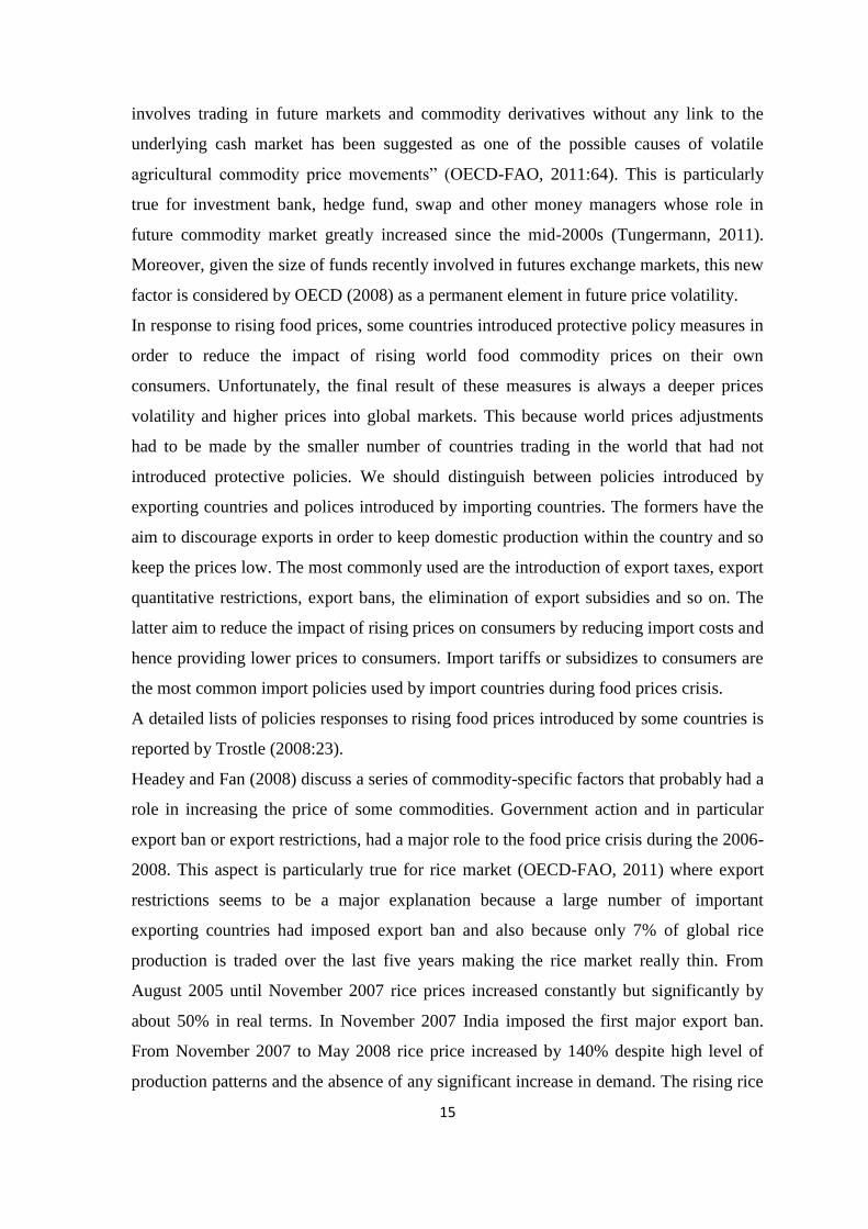
Cooke and Robles (2009) dived the explanations for the rising agricultural prices in
demand and supply-side explanations. A correlated model is the timeline of events’
model proposed by Trostle (2008) which distinguishes between supply and demand side
factors, as already seen, but also between long term factors (such as increasing demand
and slowing agricultural production), medium term factors (dollar devaluation, rising
crude oil prices, biofuels production) and short term factors (such as adverse weather and
trade shocks).
In particular the model provides eight demand driven explanations and five supply driven
explanations. Demand side explanations include the notion of rising world demand for
food products in developing countries such as China, India, Brazil and other populous
nations that have achieved a better standard life in recent years and the subsequent change
in the consumption behaviour with a larger amount of meat instead of vegetables.
Secondly, they consider the increasing production of ethanol and biodiesel from
agricultural commodities. Thirdly, they note the increasing activities and speculation in
futures markets of agricultural commodities. The fourth demand side explanation is
represented by the easy monetary policy in the US which is the basis for the weakening
dollar which in turns lead to higher prices in order to keep parities in other currencies.
Beginning in 2002, the US dollar began to depreciate, first against OECD country
currencies, and later against many developing countries. As the dollar is weak in

17
comparison to other currency it means that for importing countries is cheaper to import.
Since the US is one of the major export countries for a large range of commodities,
import countries increased their commodities demand from US adding upward pressure
on US price for those commodities, which in turn, lead to higher world price since the
world prices of exported commodities are typically in US dollars.
Supply side explanations include low research and development investments in
agricultural in the last twenty years, higher oil prices affecting key input prices and
transport, climate change and supply shocks related to weather conditions and finally
trade barriers and export restrictions imposed by some countries as a response to higher
food prices.
In term of agricultural production, Trostle (2008) shows how the annual growth rate in
the production of aggregate grains and oilseeds rose an average 2.2% per year between
1970 and 1990 while, since 1990, the growth rate has declined to about 1.3%. Similar
conclusions could be done about the growth in productivity, measured in terms of average
aggregate yield. This indicator roses an average 2.0% per year between 1970 and 1990
but declined to 1.1% between 1990 and 2007. According to Trostle (2008), the declining
in productivity may have related to the reduced agricultural research and development by
governmental and international institutions. In fact, stable food prices during the last two
decades may have provided a reduction in R&D funding levels as noted also by Hochman
et al. (2011). They state that low food commodity prices, at least since 2001, reduced
incentives for funding research and development to increase yields. However, Trostle
(2008) showed how private sector funding of research has increased the amount of
funding level but private sector research is generally oriented to cost-reducing rather than
yield-improving. In essence private sector focuses on innovation that could be sell to
producers whereas public research is generally involved in innovations that would
increase yields and productivity and would be convey to small and poor farmers for free.
The figure below provide a picture of Trostle’s (2008) time line of events model.
18
Figure 1.4: Timeline of events related to the prices crisis
Source: Headey and Fan 2010
Headey and Fan (2010) decide to modify Trostle’s timeline model adding speculation in
future markets to the original figure as short term factor from the demand side.
In order to better understand the causing of rising food prices, it would be useful to
describe a clear model of commodity prices formation. There seems to be little agreement
about how international commodity prices are formed. Despite this fact, the model
proposed by Headey and Fan (2010) seems to address the price formation in major
international grain market in a more explicit way. The model, reported in figure 1.5, is
based on the complex interaction between four main elements: supply, demand, actual
prices and price expectations.

19
Figure 1.5: Price Formation model in International grain markets
Sorce: Headey and Fan 2010
Buyers and sellers of grain, represented by demand and supply respectively, get price
arrangements based on supply and demand but also price expectation because grains are
storable commodities. Moreover, supply and demand are strongly influenced by a large
number of conditions. Price expectations themselves are influenced by current prices,
supply, demand but also grain report and futures markets. Finally, the model’s price

20
transmission includes also a range of parameters and relationships that are called
“additional factors” in the figure such as supply and demand elasticities, interaction
effects among factors and so on. In addition to the general model presented in figure 1.5,
Headey and Fan (2010:7) suggest to consider some basic facts strictly related to the
international grain markets such as:
1. Dominance of the US grain markets and importance of US specific factors. The
US is a global leading exporter in maize (with 60% of global export) and wheat
(25%) and is the third world exporter of soybean. The rice market is the only one
dominated by Asian countries. Hence, all US grain prices, but not the rice, are
quoted as international price. Because its leading position in global market export,
any event in US economy or in US grain market can be seen as a possible factors
for the food prices crisis such as the increased biofuel production, the depreciation
of US dollar and movements in commodity futures markets.
2. Degree of competition and market efficiency in the United States. The US grain
markets are highly competitive with a complex market organization based on a
sophisticated and highly reliable information service of the US Agricultural
Department (USDA) and the price discovery functions played by futures markets.
3. Seasonality and inelastic supply and demand functions. Most of grains are limited
to a single annual harvest. New supply sources can be represented only by
domestic stocks or international sources. These aspects make supply function very
vulnerable to relatively small shocks related to the level of stocks or international
sources. To be honest, this is not completely true for wheat that is much more
stable than maize for instance. As noted by Schepf (2006), there are two annual
crops for US and two counter seasonal wheat exporter in the south hemisphere.
Similarly, demand elasticity tends to be low. Changes in grain prices generally
have a little impact on retail food price and therefore little impact on grain demand
at least in developed countries. Anyway, in developing countries demand is still
inelastic because poor people have no choice. Higher grain prices force poor
people to concentrate their consume on this essential grain.
4. Peculiarity of the rice market. As said before, rice market presents some particular
characteristics. First of all, only 6% of the global rice production is exported
(Timmer, 2006). Then, the leading exporter countries are Asian countries such as
Thailand, Vietnam and India. Finally, rice is the major food staple for a large part

21
of population in Asia. This fact makes rice demand highly inelastic with
international price generally more volatile than the other grains prices but local
price much more stable because substantial existing trade barrier for import and
export.
The price formation model discussed in figure 1.4 and the description of the most
important facts related to international grain markets provide a useful background in order
to better understand the causes of prices crisis discussed in the following sections. Next
paragraphs describe in details four of the major drivers of the recent prices crisis.
1.1 Increases in the price of crude oil
International fuel and food prices are historically linked. Headey and Fan (2010) and
Tangermann (2011) note that also in the 1972-1974 crisis rising oil price was closely
related to the rising food prices. This strong linkage is confirmed by recent researches
based on econometric evidence such as in Baffes (2007), Vaciago (2008) and Balcombe
(2011) that show how oil price volatility may be used as a significant predictor of
volatility in agricultural commodities. In essence, rising in oil price affects food price
through both supply and demand sides as stated by De Filippis and Salvatici (2008). On
the supply side, Headey and Fan (2010) highlight how oil and oil-related costs of
production represent an important component of production cost of many agricultural
commodities. For instance it should be consider the huge impact in fertilizer prices, most
of which are directly derived by energy products such as natural gas or require a great
amount of energy to be produced. Moreover, the storability nature of grains means that
transport cost should be also take into consideration. According to Mitchell (2008:6), high
energy prices have contributed about 15-20% to higher export prices of major US food
commodities between 2002 and 2007. Similar conclusion were reached by Baffes (2007
cited by Gilbert 2010) that estimated the effect of higher crude oil price on rising
commodity prices as 17%. In a simulation realized by OECD (OECD-FAO, 2008) it was
shown that a 10% change in crude oil price results in a 2,3% change in wheat price and
3.3% change in maize and vegetable oil price that are more sensible to the oil price.
On the demand side, rising energy prices result in growing demand for bio-energy and
biofuel which are often cited as an important driver of the recent prices spike.

22
Headey and Fan (2010) argue that biofuels and its import surges by developed countries
have been highly significant sources of demand growth for grains. Mitchell (2008)
suggests that improved biofuels production in recent years has been the largest part of the
rise in food prices. However Gilbert (2010a) challenged this view attributing only a
modest proportion of food price rises to biofules demand. Also Baffes and Haniotis
(2010) state that biofuels account for no more than 1,5% of global area used in grain
production and for this reason biofules could not have a major role in prices crisis.
Biofuels include ethanol from corn or sugarcane and biodiesel from oilseeds or palm.
Higher energy prices have increased the biofules production which in turns has increased
the demand for food commodities used in biofuels production. Obviously, land uses
changed reducing supplies of wheat and crops used as food commodities. Mitchell
(2008:10) states that the US maize area expanded almost 23% in 2007 because of high
maize prices and rapid demand growth from ethanol production. This change in land use
resulted in a significant decline in soybean area (16%) which in turn reduced soybean
production and “contributed to a 75% rise in soybean price between April 2007 and April
2008”. On the other hand, oil seeds used in biodiesel production displaced wheat in EU
and in other exporting countries. In response to the increased demand and higher price for
oil seeds the land used in rapeseed production in the 8 largest wheat exporting countries
increased by 36% between 2001 and 2007 while the area in wheat fell by 1% in the same
period (Mitchell 2008). Moreover, biofuels have substantially contributed to the depletion
of grain stocks. Headey and Fan (2010:29) explain this stocks depletion arguing that not
only new land was diverted to maize production for ethanol but “most of the maize
provided for biofuel production came from existing land and from production that would
otherwise have been used to feed people or livestock”. The same conclusion could be
drawn for the wheat stocks in Europe.
As showed by Tangermann (2011:21) biofuels now account for a significant share of
global use of a large number of crops. “On average in the 2007-09 period that share was
20% in the case of sugar cane, 9% for both vegetable oil and coarse grains, and 7% for
sugar beet. With such share it should be not a surprise that world market prices for these
corps are now higher than they would be if no biofules were to be produced at all”
In essence, as noted by Headey and Fan (2008), biofuels has a direct influence for maize
price but can also explain price rises in wheat and rice because of substitution effects.
Several researches argue that biofuels account for 60-70% of the increase in corn prices

23
and maybe 40% of soybean price increase (Collins, 2008; Lipsky, 2008), while Rosegrant
et al. (2008) find that the long term impact of accelerated biofuel production on maize
prices is about 47%. The substitution effects on wheat and rice price is estimated about
26% and 27% respectively (World Bank, 2008). Hochman et al. (2011) provide a
complete and detailed literature report about quantitative estimates of impact of biofuels
on food commodity price calculated on the global food index varying from 6% (Hoyos
and Medvedev, 2009) to 75% (Mitchell, 2008).
Feedstock demand for biofuel production is expected to increase over the coming decade
even if at a slower rate than in recent years. Demand for cereals in biofuel production is
projected, under current policies, to almost double between 2007 and 2017 (OECD b,
2008).
Also according to the European Commission (2010:5), “the domestic use of cereals and
oilseeds in the EU is expected to increase, most notably thanks to the growth in the
emerging bioethanol, biodiesel and biomass industry in the wake of the initiatives taken
by Member States in the framework of the 2008 Renewable Energy Directive (RED)”.
However, as noted by Helbling et al (2008) biofuel industries seem to have a great impact
on food prices and a very small impact on crude oil price.
In the next paragraphs biodiesel and ethanol’s role in the recent rising food prices will be
discussed more in detail.
1.1.1 Biodiesel
Between 2001 and 2008, biodiesel production from edible oil seeds such as soybean, oil
palm and rapeseed expanded six fold from 2 billion liters to 12 billion liters (Hochman et
al., 2011).
The global leader in biodiesel production is the European Union with the 76% of the
global production in the 2006. In the same year, United States had 20% of global
production. Biodiesel is so important in the UE because the high share of automobiles
using diesel while in USA gasoline is preferred, for which ethanol is a substitute.
According to Abbott et al (2008:42), “in the USA, biodiesel produced from plant material
has enjoyed a greater subsidy (1$ per gallon) than ethanol but even with this higher
subsidy, biodiesel is not profitable as ethanol because the soy oil prices have risen to the

24
point that it cannot be economically converted to biodiesel in most circumstances”. The
same authors state that only 35% of world expansion in soybean oil use since 2004/2005
has been for fuel purpose with the rest used in food industry. In contrast, for rape seed oil,
80% of world increase since 2004/2005 has been used in the industrial category and in
particular related to the production of fuel for the European market. In essence, the
production of biodiesel from soybean oil is not an important driver of the higher
vegetable oil price because the low percentage of world expansion in soybean oil used for
fuel and also because the EU programme based on oilseed instead of soybean oil. In fact,
according to the European Commission (2010), the medium term prospect for the EU
oilseed markets shows a positive picture with a very strong demand and high oilseed oil
prices which lead to both yield growth and expanding oilseed area with some reallocation
between crops.
1.1.2 Ethanol
Between 2001 and 2008 production of ethanol from maize and sugarcane more than
dubled from 30 billion litres to 65 billion litres (Hochman et al., 2011). For ethanol the
global leaders are USA and Brazil with a percentage of global production in 2006 around
37% for both countries (Abbott et al, 2008). USA ethanol derives mainly from corn
whereas Brazil uses sugarcane.
Mitchell (2008) observes that Brazilian ethanol production has not contributed
appreciably to the recent increase in food commodities prices because Brazilian sugar
cane production has increased rapidly and sugar exports have nearly tripled since 2000.
Only half of Brazilian sugar cane production is used in ethanol industry for domestic
consumption and export, the other half is used in sugar production. More in detail the
sugar production increases from 17.1 million tons in 2000 to 32.1 million tons in 2007.
In the USA ethanol has been subsidized since 1978. At the beginning, with the price for
the crude oil ranged between 10$ and 30$ per barrel with some exception, the subsidy
was fundamental for the ethanol industry to grow slowly. Abbott et al. (2008) state that
without the subsidy ethanol would have been profitable only with the crude oil quoted
above 60$ per barrel. Also IFPRI (2007), Headey and Fan (2010) and Schmidhuber
(2006) calculated that when oil prices range between US $60 and $70 a barrel, biofuels
are competitive with petroleum in many countries, even with the existing technologies.
When oil prices are above US $90, the competitiveness is of course even stronger. Since

25
2004, crude oil price has been changed drastically increasing from 60$ in April 2006 to
120$ in May 2008. The high oil price, in addition to the subsidy and low corn price until
2008, lead to a huge investment in ethanol production, which in turns lead to a higher
demand for corn. But this increased demand for corn used to produce ethanol led to
higher prices in corn as a final result.
A large strand of literature (Abbott et al , Headey and Fan 2010, Schepf 2008, Von Braun
2008) concludes that the diversion of the US maize crop from food to ethanol uses
represents one of the most significant demand-factor of rising food price.
According to Mitchell (2008) between 2004 and 2007, 70% of the increase in global
maize production was used for ethanol. In the same period, ethanol use grew by 36% per
year while feed use grew only 1.5% per year.
The use of maize for ethanol especially in US has important global implications because
the strong position of US in global maize production (about one–third) and its leadership
in global maize exports (about two-thirds). Mitchell (2008) states that the US used about
25% of its maize production in ethanol.
It is not an easy task to estimate the contribution of biofules, and in this case ethanol, to
food price increases. In fact, estimates can differ in a wide way in function of different
length of time considered, different prices considered such as export price, retail price,
food product, currency and so on. Moreover, using general equilibrium model instead of
partial equilibrium would lead to different estimates. Despite all these different
approaches, many researches recognize biofuels as a fundamental driver of food prices.
The International Monetary Fund (IMF) cited by Headey and Fan (2010) estimated that
the increased demand for biofuels accounted for 70% of the increase in maize prices and
40% of the increase in soybean price (Lipsky, 2008). Collins (2008) estimates that about
60% of the increase in maize price from 2006 to 2008 have been due to the increase in
maize used in ethanol production. Also Rosengrant et al. (2008) quoted by Mitchell
(2008) calculated that, because of increased biofuel production, maize price have
increased 21% in real terms, wheat prices increased 22% and rice prices almost 21%.
The important contribution of biofuels in food prices crisis raises pertinent policy issues
about the opportunity to carry out with US and EU government policies based on
subsidies to biofules production.
Anyway, Abbott et al. (2008:44) state that, at present, most of the corn price increase is
related to the higher oil price and only for a little part due to the subsidy. In other words,

26
“as oil has increased, corn-based ethanol is demanded to substitute for gasoline. At high
oil price, this would happen with or without the subsidy.” Removing the subsidy does not
decrease the corn price until the oil crude price fell as well. Despite of this, a study by the
Food and Agricultural Policy Research Institute (FAPRI) reported by Headey and Fan
(2010) estimates that the joint implementation of both subsidies and tax credits for
ethanol supports maize prices by about 20%.
Despite of this large strand of literature in favour of the so called “fuel vs food debate” a
recent work by Bastianin et al. (2013) analyzes the relationship between the price of
ethanol and agricultural commodities using data from Nebraska which is deeply involved
in ethanol production. In their piece of research the authors used advanced statistical
techniques to define long run relation and Granger causality linkages between ethanol and
the other commodities. The findings of this study show no evidence to state that ethanol
price should be considered a long run driving force for the price of food commodities.
Finally, biofuels lobby groups argue that the role of ethanol as a driver in rising food
prices is overestimated. In fact they point out that ethanol production uses only the starch
in maize. Hence, maize oil and protein could still used in animal feed system.
1.2 Exchange rates and us dollar depreciation
Commodities prices increases not only because of supply-demand events in individual
markets but also because of macroeconomics events that changed the environment within
the markets find their own equilibrium. The common literature considers different
macroeconomic variables to explain prices increase. The exchange rate and the US dollar
depreciation is one of the most analysed variable. A large number of recent studies cites
the depreciation of US dollar as one of the major causes of current high commodity
prices. Few of these studies, as it will be seen, try to quantify the role played by dollar
depreciation in commodity prices crisis. Generally speaking, when the dollar is weak,
agricultural exports and in particular grain and oilseed exports grow. Since the US dollar
is used in the international trade of agricultural commodities, it should be clear that a
depreciation of the US dollar lead to higher prices in the United States but, at the same
time, lower prices for the rest of import countries. Before analysing the relationship
between exchange rate and commodities price, it would be useful introduce some

27
background on dollar depreciation in order to better understand its real impact and role in
commodities price increase. According to Abbott et al. (2008), the recent dollar
depreciation is surely related to the huge trade deficits that the United State is still
realizing. In fact the authors state that the US trade deficit reached the record of 5.75% of
GDP in 2006. In the 2007 the depreciation of dollar brought some small improvement
leading the deficit to the value of 5.1% of GDP. Between 2006 and 2007, the increased
agricultural export was a significant contributor to the small improvement in the trade
deficit. The higher agricultural commodities price had an important role in diminishing
the US trade deficit. On the other hand, the depreciated exchange rate, resulting in smaller
prices increases in the rest of the world, have sustained the export quantities in the face of
higher US price. However, the trade deficit is well linked to a capital account surplus as
money from OPEC and China flows to finance the US deficit. The IMF (2007, cited by
Abbott et al 2008) noted that OPEC investment in the US economy and Chinese treasure
bill purchases were fundamental to keep up the dollar’s relative strength until the recent
financial crisis and the subsequent interest rate cuts. The dollar depreciation was also
worst after the Fed interest rate cuts. Vaciago (2008) provides a complete view on the
monetary expansion policy applied in US and in other important developed countries, the
low rate of interest that increased the amount of money and subsequence depreciation of
US dollar showing how these aspects lead to the rising food prices.
For how long the US dollar is going to stay weak will depend on several factors such as
the confidence of foreign investors in the US economy, the increases of export due to the
US dollar depreciation and the decrease of import, the extend of inflation and finally
interest rate in US and abroad.
Since 2002 to 2008, corn prices in nominal dollar have increased 143%. In real Euros the
increase is only 37% (Abbott et al, 2008). In the 1995-96 a similar price run-up
experienced a nominal $ increase near to 143% and a real Euro increase of 94%. The
comparison between the 1995-96 prices crisis and the recent price increase lead to
conclude that in the former the corn price increases were due in an extensive part to
supply and demand balances with exchange rates playing almost no role, while the latter
looks quite different with dollar depreciation playing a much more important role in price
increases.
More in details, the US dollar depreciated against the Euro about 35% from January 2002
to June 2008 and the depreciation of dollar has been shown to increase dollar commodity

28
prices with an elasticity between 0.5 and 1.0 (Gilbert 1989). Cooke and Robles (2009)
using data from Federal Reserve Branch of St.Louis, show a US dollar depreciation
against euro close to 65% since 2002.
Mitchell (2008) calculated that the depreciation of the dollar has increased food prices by
about 20%, assuming an elasticity of 0.75. Abbott et al. (2008), using USDA’s
agricultural trade-weighted index of real foreign currency per unit of deflated dollars, find
that from 2002 to 2007 the US dollar depreciated 22% and the value of agricultural
exports increased 54%.
1.3 Speculative and investor activity
During the recent prices crisis it has been argued (Baffes and Haniotis, 2010) that
fundamentals have played a major role in commodities prices crisis but demand and
supply considerations are not enough to completely explain the prices boom. Many
researchers and analysts argue that excess liquidity and speculation have to be taken into
consideration. Various aspects related to speculation have been discussed. In particular;
excess liquidity, index funds activity, speculation, the role of commodity futures
exchanges and speculative bubble have received more attention than others. Obviously,
the complexity of each aspect and the interrelationship between them has led to different
conclusions and mixed results about their role in rising food prices. The next paragraphs
of this section try to summarizes some of these results.
1.3.1 Excess liquidity and index funds activity
Baffes and Haniotis (2010:6) note that the low interest rate environment supported by
many central banks lead to an excess of liquidity, part of which was invested in
commodity markets. Low interest rate represents only one of the three sources of new
money that found its way into commodities markets. The same authors suggest
diversification of investment vehicles and rebalancing of investment portfolios as other
sources for “new money”.
The former is related to the investment funds managers searching for new and
uncorrelated assets. Thus, funds managers began to invest in commodities, including
agricultural commodities, just to diversify their investments into uncorrelated assets. The

29
rebalancing of investment portfolios towards commodities added further inflows into
commodity markets. The effect of this rebalancing is less permanent than diversification
and depends on investors’ risk attitude.
The key investment vehicles for this new money into commodity markets are index funds.
The Down Jones-AIG and S&P Goldman Sachs Commodities Index (also known as DJ-
AIG and S&P-GSCI) are the two most used indices. According to Baffes and Haniotis
(2010), about 95% of funds indexed to commodities are replicated by these two indices.
The funds buy long position contracts in commodities futures markets exchanges and,
prior to expiration, rolling them over. Romano (2009) calls them long-only commodity
index funds.
Baffes and Haniotis (2010) report that there are not a precise estimates on the funds’ size
but a realistic range seems to be $230-240 billion in 2009. Although these amount of
money represents only one percent of the global value of pension and sovereign wealth
funds holdings, they are really large in comparison to the size of commodity markets. In
essence the effect of the new money on commodities prices has been associated with
speculation and subsequent price bubble. However, the view on this subject have been
quite extreme and still under debate. In order to better understand the core of this debate
in the next paragraphs it will be discussed what speculation is and the mechanism of
commodities trading activity in futures exchanges.
1.3.2 Speculation
A large strand of literature have suggested speculation in commodities future markets as
one of the major cause of rising food prices. However, the recent debate on speculation
shows extreme positions of opinion leaders and insufficient and not always clear
empirical evidences. This extreme complexity on the subject partly reflects the different
types of “speculative activity” that analysts and economists refer to. Indeed, in order to
understand the complexities of speculation it will be discussed the different sources of
speculation, the place where transactions take place, the actors involved and their
motivation.
As suggested by Baffes and Haniotis (2010), the traditional separation of the place in
which transactions take place (physical versus financial) and the actors involved (hedgers
versus speculators) does not exist anymore. A more complex picture should be now

30
considered with speculators engaged in financial transaction but also in physical
transactions by holding inventories and, on the other hand, hedgers involved in physical
but also financial market transactions.
1.3.3 Actors involved
The hedgers include producers and consumers both involved in physical transaction of
commodities. These are called commercials in Commodity Futures Trading Commission
(CFTC) terminology. They have an exposure to the price of the physical commodity that
is long in the case of producers and short in the case of consumers (processors). They are
used to offset their positions (at least partially) by taking an opposite position in the
futures market. Behind the hedgers two more actors should be considered that operate
with pure financial motivation and are not involved in physical markets transaction:
Speculators and investors. Speculators are often trend followers. They may take long and
short positions but they hold positions for only short periods of time. Hedge funds and
commodity trading advisors (CTAs) are typically included into this category.
In particular, hedge funds are involved in a large range of asset including commodity
markets. A hedge fund may invest in commodity markets mainly to “hedge” the diverse
risks of their portfolios.
In such a case, investing in commodity markets represents an investment in a
non‐correlated asset that provides diversification benefits to the overall portfolio. Hedge
funds are not new instruments and they may have short term effects on commodity prices.
Commodity trading advisors (CTAs) are asset managers that operate almost exclusively
in commodity markets looking for profits from market volatility. For this reason, CTA
activity is thought to reduce price volatility since they trade on the basis of market
fundamentals and technical analysis.
The third category of actors involved is represented by investors. They take usually long
positions in commodity futures market in order to diversify their portfolio. During the
past few years, as said before, this class of actors generally called investment funds and
including pension funds and sovereign health funds have dramatically used financial
markets’ products. According to Baffes and Haniotis (2010) investment funds include
sovereign wealth and pension funds. As said before, in the few past years they began
including commodities in their portfolio mix in order to diversify with uncorrelated
31
assets. The major concern about investment funds is represented by their relative size
compared to commodity markets and the subsequent possibility to unbalance the markets
itself. Soros (2008) asserted that investment in instruments linked to commodity indices
had become the “elephant in the room” and stated that investment in commodity futures
might exaggerate price rises.
1.3.4 Place of transaction
Commodity transactions take place either in physical market or in future exchanges
board. Futures markets evolved gradually during the last century. At the beginning,
commodities exchange were mostly cash markets where physical commodities were
bought and sold. As the volume of trading increased, buyers and sellers began trading
forward contract. This type of contract can be defined as an agreement in which a seller
agree to deliver a cash commodity to a buyer sometime in the future. In essence, quality,
quantity, delivery time and location, as well as the price, are defined in advance. The
advantage of cash forward contract in comparison with an immediate cash sales
transaction is that it allows both buyers and sellers to know in advance the price of the
specific commodity. Moreover, they can postpone delivery until they have possession of
the grain (sellers) or they are ready to process it (buyers).
Nevertheless, forward contracts presented different negative aspects. First of all they are
privately negotiated. Secondly there are some risk to both parties in the agreement. One
side may negotiate in bad faith or without sufficient funds or may not able to fulfil the
contract. In order to avoid these problem and make easier and safer the transaction in
1865 the Chicago Board of Trade (CBOT) introduced the first standardized commodity
futures contracts. Futures contracts are standardized and meet specific requirements of
buyers and sellers for a variety of commodities (not only agricultural commodities) and
financial instruments. With this contract, quantity, quality, delivery locations are
previously established. The only variable that is not fixed yet is the price, which is
discovered through a kind of auction process on the trading floor of an organized futures
exchange.
Currently, Chicago Mercantile Group (CMG), which is the sum of the Chicago Board of
Trade and the Chicago Mercantile Exchange, is the world’s largest market place for
trading futures and options. In 2007 it saw trading volume of 2.2 billion contracts with

32
three-quarters of the traders executed electronically. The huge and increasing use of
futures contracts is due to the standardized terms and the possibility to offset them.
Commercial firms realized that future markets could provide financial protection against
price volatility whereas speculators found that, thanks to the standardize terms, futures
contracts could be bought and later sold in order to achieve some profit with correct
forecast of price movement. In this case, the risk is transferred to hedgers form
speculators. In essence, risk transfer and price discovery power are the two major benefit
of futures contracts markets.
Despite of these benefits, there are different concerns about futures contract. First of all,
futures contract allow a large number of so called non-commercial participant to take part
in trade. Non-commercial participants are all those who are not directly involved in
agricultural production, distribution, and delivery to markets. Us Commodity Futures
Commission gradually changed the roles over who may trade in agricultural futures
leading to a greater index funds participation in future markets. Headey and Fan
(2010:41) accounted the index funds participation for almost 40% of the futures contract
trading in wheat in 2008. The figure below show how massive has been the investment of
commodity index funds during the last decade.
Figure 1.6: Commodity index fund investment in billion US dollar.
Source: Barclays cited by Irwin and Sanders (2010b).

33
The concern about this is that non-traditional participants can now speculate on food price
trends since futures contracts value varies in relationship to the commodity spot prices
market. In essence, the variation of commodity prices is an opportunity for the
speculators to bet on futures contracts just like for any other asset class. So, as
summarized by Headey and Fan (2010), a short futures position (referred to contracts
within 6 months) protects against price decreases, whereas long position (involving
contracts of longer than 6 months) may benefit from price increase in long term run. Most
commercial agricultural traders play in short futures market but most non-commercial
player, the so called speculators, prefer long term position. Hence, a common measure to
quantify speculative activity is based on long term market contracts such as the share of
long position taken by index funds.
1.3.5 Speculative influence on commodity futures price
Cooke and Robles (2009) use a large range of proxies for participating in agricultural
commodity futures markets and in speculative activity such as the volume in futures
contracts, open interest in futures contracts, the ratio of volume to open interest in futures
contracts and finally the amount of positions in futures contracts by non-commercial
traders.
In particular, the monthly volume in futures contracts indicator expresses the total number
of trading on a commodity futures contract in the Chicago Board of Trade (CBOT) on a
monthly basis. According to the authors, in recent years traded volumes in futures
contract in agricultural commodities have deeply increased until 2008. In 2006 the
average monthly volume in futures for wheat and corn grew by more than 60% with
respect to the previous year. In 2007, volumes grew significantly for all the most
important commodities with a monthly average 40% larger than in 2006. Monthly open
interest in futures contracts has also grown between 2003 and 2008 with great differences
in function of the commodity considered. The last two indicators studied by Cooke and
Robles (2009) are the Ratio of volume to open interest in futures contracts and the
importance of non-commercial positions in futures contracts. The former is used to
capture speculative market activity under the assumption that a speculator prefers to buy
or sell contracts on a short period of time increasing the monthly volume in futures
contracts without affecting the monthly open interest in futures contracts. The results

34
achieved by the authors show how the increasing of the ratio would be interpreted as a
potential speculative behaviour between 2005 and 2008. The latter indicator (importance
of non-commercial positions in futures contracts) represents an amount of the speculative
activity in search for financial profits. The importance of the non-commercial position is
expressed as the ratio of non-commercial position to total positions. According to Cooke
and Robles (2009) this ratio seems to be growing during the period of time studied. For
corn they report that the ratio for long position only was on average 0.29 in 2005, and in
the first five months of 2008 it reached an average of 0.49. In the case of short positions
there is less evidence of upward trend of the ratio. Since both commercial and non-
commercial increased their participation in the futures market. Hence, Robles and Cooke
(2009) find an econometric linkage between futures market activities and spot market
prices using time series analysis. They conduct 23 tests with four different commodities
and proxies for speculative activity described before providing evidence that financial
activity in futures markets and proxies for speculation can help to explain the observed
change in food price . Their results show evidence of Granger causality in 6 of the 23
tests. Finally, they try to explain the relationship between speculation and spot price
arguing that in agricultural futures markets producers try to hedge their futures income
selling short, whereas industrial processors take long position hedging their costs. The
volume of these two different positions does not always match and hence non-commercial
or speculators traders play the important role to provide liquidity to the market closing the
gap between the two positions. However, when speculators activity increase significantly
on both sides of the market this may affect spot prices. In essence, if a large groups of
speculators take part to the market with long position betting on higher future spot prices,
futures price may be driven upward up to the point they start to attract further speculators.
At this stage, signals for higher prices are transmitted to the spot market confirming the
expectation of higher prices and providing positive feedback on further expectations.
Romano (2009) calls this step as self-fulfilling expectations.
Similar conclusions have been reached by a large strand of literature providing theoretical
and empirical evidence on how speculation has contributed to the crisis.
Gheith (2008), Masters (2008), Masters and White (2008) assert that speculative activity
by index funds create a “bubble” with the result that commodity prices (but also crude oil
price) was not driven by only fundamental values. Masters (2008) clearly stated that
“Institutional Investors are one of, if not the primary, factors that contribute to price

35
determination in the commodities markets”. Soros (2008) defined commodity index
trading as potentially destabilizing for their relative size compared to the commodity
markets size. Calvo (2008) stated that commodity rising prices are the result of
rebalancing of investment portfolios by index funds. He also noted that speculation
activity and low inventories are not necessarily inconsistent with each other challenging
one of the major motivation of speculation thesis’ opponents as it will seen later. Plastina
(2008, cited by Baffes and Haniotis 2010) highlights the role of investment fund in rising
cotton price between January 2006 and February 2008. Finally, Gutierrez (2012), using a
bootstrap method, provides evidence of explosiveness in the future prices of wheat and
rough rice in 2007-2008.
However, the impact on price is hard to quantify and most studies do not find that such
activity changes prices from the levels which would have prevailed without speculation.
In essence, to provide theoretical and empirical evidences showing the role of speculation
in prices crisis is not an easy task. A large school of thought highlights logical
inconsistencies in the arguments proposed by bubble proponents and several observed
facts that challenge the speculation proponents’ theory. Krugman (2009) challenged the
belief that speculation was a major factor in rising prices and also rejected the idea that
commodity trading in futures exchange may have influenced commodity prices arguing
that a future contract is a bet about the future price without direct effect on the spot price.
Wolf (2008) stated that inventories were low during the rising price and this fact is in
contrast with the speculation activity since in presence of speculation, one would expect
to see commodity inventories increase. Similar conclusion has been reached by Wright
(2009) that noted that if long futures positions were behind the grain price boom in 2008,
stocks would have increased. Two IMF studies (2006, 2008) cited by Baffes and Haniotis
(2010) found no econometric empirical evidence that speculation had a role in rising
commodity prices.
Irwin et al. (2009) and Sanders and Irwin (2010) challenged the conclusion that
speculation has influenced agricultural futures prices leading to a bubble price. They both
review the theory and the evidences against the main role of speculation in rising food
prices adding new data and empirical analysis. In particular they discuss three conceptual
errors, that reflect fundamental and basic misunderstandings of how commodity futures
markets actually work, and five logical inconsistencies with the arguments of bubble
proponents. The first and most fundamental conceptual errors challenged by the authors is
36
to equate money flows into futures markets with demand. Investments into long or short
position of futures markets in not the same as demand for physical commodities. “With
equally informed market participants, there is no limit to the number of futures contracts
that can be created at a given price level” (Sanders and Irwin 2010:26). Index funds long
positions should be considered as new “demand” such as, at the same way, index funds
short positions should be considered new “supply”. In essence, put in this way, money
flows do not necessarily impact prices. It should be clear that this argument is true only if
all the participants are perfect informed. If this is not the case, it is possible that a huge
increase in long side positions should be interpreted by some trades as a result of reliable
private information about commodity prices evolution. Anyway, because the publicity
about index funds buying activity and because trading methods is very transparent, the
authors consider highly unlucky that something like that would happen in a wide enough
scale to drive prices out of fundamentals.
The second conceptual error is to state that index funds affect futures and spot commodity
prices since they only participate in futures markets. More in detail, in the short-run,
commodities prices are defined in the futures markets and translated from futures to spot
markets. However, in the long run, equilibrium prices are only discovered in the cash
markets where demand and supply of physical commodities reflects fundamental forces.
As also reported by Headey and Fan (2008), index funds do not participate in the futures
delivery process or in the cash markets or in the purchase of the cash commodity. “Index
investors do not participate in the futures delivery process or the cash market where long
term equilibrium prices are discovered” (Sander and Irwin 2010:26). Irwin et al. 2009
observe that in order to affect the equilibrium of commodities in the spot markets, index
funds would have to take delivery and hold these stocks off markets. By the way, there is
no evidence that index funds have been involved in delivery or hoarding process.
A third conceptual errors made by speculative bubble proponents is a scholastic and
unrealistic definition of hedgers and speculators. Usually, hedgers are seen as risk-
avoiders whereas speculators are considered active risk-seekers. This basic distinction is
no any more in line with the most common literature that better describe the behaviour of
hedgers and speculators as a continuum between pure risk avoidance and pure
speculation. Moreover, many commercial firms labeled as hedgers speculate on prices
direction whereas some speculators are engaged in hedging activities. In other terms
index funds investments into commodity futures markets did not disturb the perfect

37
equilibrium between hedgers and speculators, but instead the funds entered into a
dynamic a much more complex equilibrium between commercial firms (hedgers) and
speculators with various motivation and strategies that cannot be defined simply as risk-
avoiders or risk-seekers.
In addition to these conceptual errors, Irwin et al. (2009) and Sanders and Irwin (2010)
describe five facts about commodity markets that are clearly inconsistent with the
arguments of bubble proponents. Firstly, the statistics on index funds investment tend to
focus on absolute position size and activity. A quantification of speculation activity
should be done always in relative terms comparing speculative activity to hedging needs.
Sanders et al. (2008) demonstrate that the level of speculation in nine commodity futures
markets from 2006 to 2008 was not excessive but within the historical levels. In essence,
the rise in index funds activity was more than offset by commercial participation.
The second inconsistent fact is that if it is true that index funds buying drove commodity
prices higher, then markets with the highest concentration of index funds positions should
have registered highest prices increase. Despite of this, Sanders and Irwin (2010) show
how the size of index funds investments in different markets is not strictly correlated to
the prices movements. They show how future market with the high index funds
investments such as livestock markets had little or no prices increase, whereas other
markets with lower level of index funds participation such as grains and oilseeds
registered the largest prices increases.
A subsequent inconsistent fact, also observed by Headey and Fan (2008) is that high price
were discovered in commodity markets not connected to index funds investments such as
rubber and onions for instance. This would suggests that other macroeconomic factors
may influence commodities rising prices.
The fourth inconsistent fact is related to inventories for storable commodities. The
theoretical market equilibrium occurs when supply and demand curves intersect. The
result is the equilibrium price. If we admit a bubble in the market, the new price is now
above the equilibrium price. It means that at the bubble price the quantity supplied exceed
the quantity demanded as showed in the figure below.

38
Figure 1.7: Theoretical impact of a price bubble in a storable commodity market
Source: Irwin et al (2009)
It should be expected an increase in inventories when bubble is present in a storable
commodity market. Nevertheless, the level of stocks for corn, wheat and soybean
decreases since 2005. By the way, Gilbert (2010:408) argue that even if this argument is
correct “it may take time to play out”. In the case of food commodities, with the inventory
supply curve near vertical in the short or medium term, the increase demand can only be
met by an increase in the cash price.
The last inconsistent fact is related to the nature of commodity index trading. Theoretical
models show how a group of uninformed traders (the so called “noise traders”) can
significantly drive prices away from fundamental values making a gap between market
prices and fundamental values. In the case of index funds, it is highly unlikely because
the transparency of commodity index trading. In fact, they are used to publish their
portfolio (market) weights and roll-over periods. In essence, index funds do not attempt to
hide their current position nor their next moves. Hence, if index funds drive prices away
from fundamental values, other large rational traders would trade against index funds.
Despite this fact, as reported by De Long et al. (1990 cited by Gilbert 2010), informed
traders may push away from the fundamental values rather than to return to fundamental
if they have a short time horizons.

39
Sanders and Irwin (2010) provide an empirical test of this inconsistent fact using data
from Commodity Futures trading Commission (CFTC)’ report1. In particular, the authors
test if the relative index funds participation is correlated to subsequent returns across
markets analysing the relationship between index funds positions and returns across 12
commodities futures markets. However, using both Fama-Macbeth method and traditional
cross-sectional tests, the null hypothesis of no cross-sectional impact (it means that index
fund positions do not impact returns across futures markets) is only rejected in one of 12
models.
Moreover, Irwin and Sanders (2010) fund not only a negative Granger cause relationship
between index funds positions and market return but, more important, a statistically
significant negative relationship between positions and market volatility. In other words
the authors show consistent evidence that increases in index trader positions are followed
by lower market volatility. Anyway, they also suggest to interpret this result with great
caution. In fact, another third variable not included in the model could be involved in
market volatility decline.
Gilbert (2010b), using data from the CFTC’s Supplementary Commitments of Traders
reports for twelve agricultural futures markets which distinguish positions held by index
providers, indicates that index-based investments in commodity futures markets may have
been responsible for a significant and bubble-like increase of energy price, although the
estimated impact on agricultural price is smaller. In the case of agricultural commodities
the maximum impact may have been to rise prices by the order of 15%.
In conclusion, Baffes and Haniotis (2010:9) argue that any financial activity related to the
commodity markets is unlikely to affect the long term price trends which is ultimately
influenced by market fundamentals. In essence there should not be any linkage between
rising spot prices and rising futures prices. However, “such activities can induce higher
price variability as the most likely did during the perfect storm of 2007/2008”. This
conclusion is supported by Headey and Fan (2008:379). They conclude that “futures
markets are unlikely to be a leading cause of the overall price surge, since there is little
evidence that these markets significantly influence real supply and demand factors”. The
same authors admit the possibility that futures markets may have only exacerbated the
volatility in agricultural markets showing how the contract price volatilities of corn and
1 CFTC’s Commodity Index Traders

40
wheat futures price indexes have increased from 19.7% and 22.2% since 1980 to 28.8%
and 31.4% in 2006-2007, respectively (Schnepf, 2008). This positive trend for volatility
has been observed also by Sarris (2009) using historical yearly cash price volatility index
of Chicago Board of Trade (CBOT). Thus, speculation may be more a symptom than a
cause of underlying volatility. When markets are flat, futures contracts tend just to reflect
the discounted future value at today’s prices but when markets are in turmoil,
expectations of future prices may vary considerably opening rooms for speculation (CBC
2008).
1.4 Decline of commodity stocks
Besides the above mentioned factors, the list of possible causes analysed in the recent
literature includes the decline of commodity stocks (Abbott, Hurt and Tyner, 2008).
Economic theory has described how commodities stock can play a main role in buffering
price volatility. The theoretical background, as we’ll see later in details, includes the
pioneering works of Gustafson (1958), Samuelson (1971), Wright and Williams (1982,
1984), Scheinkman and Schechtman (1983), Williams and Wright (1991) and Deaton and
Laroque (1992). All these authors focused on the competitive storage model under the
assumption of rational expectations showing how stocks are a key factor in commodities
price behaviour. In essence, storage model states that storage building can mitigate
demand and supply shocks. On the other hand, low level of stocks will increase price
volatility.
Starting on 1999/2000, the global stock level for major cereals has been declined. In
2007, world stocks of cereals, expressed in terms of stocks to use ratio, had reached its
historically low level (Dawe, 2009; Wright, 2011) even in comparison to the levels
reached in the early 1970s food crisis (Tangermann, 2011). For both events, 1973-1974
and 2007-2008, the literature has generally recognized the critical role of commodity
stocks. Piesse & Thirtle (2009) argue that the single most important factor in agricultural
prices was low inventories. The stocks/utilization ratio for grains and oilseeds dropped to
15% in 1972 and 1973 and did not touch such a low level again until 2008. Trostle (2008)
recognizes the importance of fundamental supply and demand factors, emphasizing the
decline in stocks to use ratio for wheat, rice and corn grains leading up to the boom
witnessed in 2008.

41
Indeed stocks have played an important role in price stabilization policies in the past and
remain a core topic today in discussions about achieving food security. For example, the
announcement of the release of Japanese rice security stocks is thought to have acted as a
depressant during the rice spike (Dawe, 2010). Therefore, it is not surprising that the
usefulness of holding public stocks has been the subject of debate by scholars in recent
years (see Timmer 2010, and Von Braun & Torero 2009).
The level of stocks represents the difference between output and use. The low level
simply reflects that since 1985 to 2007 the worldwide demand for cereals had been larger
than the worldwide supply. The decline in inventory resulted in commodity prices being
more sensitive to any given shock.
The decline in global cereals stocks just before the price spike was due to different
factors.
First of all, unfavourable weather conditions reduced cereals productions in some
important exporters countries. Moreover, the shortfalls in output coincided with a
continued growth of global use (Tangermann, 2011).
The low stock levels observed in recent years have been also attributed to policy
adjustments of price support and intervention purchase schemes in some OECD countries,
as well as to correction of the quality of information on private and government held
stocks in important producing and consuming countries. Tangermann (2011) notes that
both China and EU have changed their storage strategy reducing the minimum required
levels.
Moreover, overall demand for food and feed due to economic growth and population
growth, at least in developing countries, and demand for biofuels, especially in developed
countries, accompanied by slow rates of increase in output because declining productivity
growth have meant demand exceeded production since 1985 leading to the lowest level of
stocks.
All these factors, resulted in a decline of stock to use ratio of world grain and oil seed
stocks from 35% in 1985 to less than in 15% in 2005 (Trostle, 2008). In essence, during
the last 25 years, stock to use ratio declined by more than 50%.
When stocks are depleted, commodity price become highly linked to information on
stocks. On the other side, when stocks are in abundance price volatility is historically low.
In other words, stockholding behaviour provides an important clue to expanding
commodity booms and busts, along with other fundamental factors such as supply and

42
demand shocks. Tangermann (2011) shows how when stocks are low, many agents may
be nervous and change their rational behaviour. For instance, in expectation of rising
price, farmers may sell their production a little bit later and, on the other side, traders,
processors and distributors may buy a little bit earlier. The result of these change in
behaviour is that a higher quantity of the involved commodity can get absorbed in the
food chain in comparison to a normal condition represented by a normal volume in stock.
Also importers may adjust their buying behaviour. Trostle (2008) has observed that by
late 2007, when commodity prices were in their spike, some importers were buying larger
volume in order to cover their need for a longer period of time (5-6 month instead of 3-4
month).
While much discussion has been held on the main role played by stocks in food price
crisis, however, empirical literature has, so far, provided only little attention to this topic
mainly because the scarcity of empirical data on public and private stocks.
Kim and Chavas (2002) have found results that are consistent with the theory of
competitive storage model under rational expectation for the US not-fat milk market.
Balcombe (2011) analysed the volatility of different world agricultural prices showing
how volatility can be also explained by stock levels having a downward impact on
volatility. He noted how when stocks are low, the dependence on current production in
order to meet short-term consumption demands is likely to rise. Even small shocks to
supply may have a severe dramatic effect on prices. Similar results have been obtained by
Stigler and Prakash (2011) using a two stage analysis in the US wheat market.
In line with these empirical results, Cartel et al. (2011) state that high levels in storage
provide a buffer against supply and demand shocks. In response to such shocks,
inventories can be depleted, mitigating the impact on prices. When inventories are low,
the lack of a buffer leaves the markets vulnerable to price spikes. Not only low stocks are
important in order to increase volatility price but also uncertainty about stock levels in
some parts of the world and even expectations of depleted stocks may lead prices to rise
sharply.
Hochman (2011) developed an empirical model that also included crop inventory
adjustment behind the most common drivers for the price spike in 2006-2008. His
research shows that, if inventory effects are not taken into account, the impacts of the
various factors on food commodity price inflation would be overestimated showing, in
this way, the important role of storage in explaining the price crisis. Finally, Serra and Gil

43
(2012) showed how stock to disappearance forecast has a key role in corn price instability
in line with the competitive storage theory by using a MGARCH model which is
estimated both parametrically and semi-parametrically.
However, no consensus has yet be reached on the role played by low stocks level during
the 2006-2008 price crisis. Several economists remain less than convinced about the
empirical importance of stock depletion and the relationship between high price and low
stocks level, both in the short and long term. For instance, Dawe (2009) concludes that
the link between volatility and world rice stock levels was rather weak during the 2006-08
event. Roache (2010), who used data from the last one-hundred years, came to similar
findings showing that long-term volatility in commodity prices is not influenced by
commodity stock levels.
Thus, to explain commodity booms and busts, we need an understanding of what
determines stock levels and, in particular, what may cause inventories to be depleted. In
order to do this, next chapter will provide a deep description of the competitive storage
model, which views inventories as the main determinant in commodity price behaviour.

44
2. THE STORAGE MODEL
2.1 Introduction
Large volatility in output and prices are key features of agricultural commodities markets.
A clear understanding of storable commodity prices’ dynamics and the relationship
between prices and the fundamentals of supply and demand is yet to be reached. The
recent periods of prices crises and extreme volatility has stressed the need to better
understand the characteristics of price dynamic in order to construct good policy. The
need to understand the complexity of commodity price dynamics has became even more
urgent against the recent tendency to remove traditional governmental stabilization
schemes. A plethora of potential methods of studying large fluctuations in output and
prices for agricultural markets have been developed since the Great Depression of the
1930s. Obviously, volatility implications are strictly correlated to the assumptions
assumed about consumption demand, supply curve, risk aversion and the nature of other
fundamentals. The traditional and easier approach to market stabilization issue is often a
simple and static supply-demand analysis. Storage implication and the effects of storage
interventions in subsequent periods are typically ignored or, in the better case, broadly
estimated in spite of the abundance of storage examples in nature. Nevertheless, many
econometric models have stressed the role of commodities storage starting with Allen
(1952) who defined an explicit demand curve for inventories as function of current price.
In other empirical models, such as Lovell’s (1961), firms adjust inventories slowly toward
some optimal level. Bivin (1986) challenged this approach for not being obtained from
any optimization behaviour. However, there is a theory about commodity price behaviour
including storage effects that tends to dominate: the storage model. This model has a long
history moving from the contribution of Gustafson (1958) who studied the properties of
the optimal demand for commodity stocks, and with the work of Muth (1961), who
introduced the assumption of rational expectation. During the last twenty years, the basic
model has been implemented in several different directions. Samuelson (1971) and
Scheinkman & Schechtman (1983) extended the model including the effects of economic
incentives on supply function. Williams and Wright (1991) made a deep exploration of
the model and its economic implications extending it in many important directions
including the effects of speculative attacks and government interventions. Williams and

45
Wright (1991) highlighted the endogenous nature of the demand curve for inventories as
function of current price. In essence in their model the collective level of inventories is an
endogenous variable in contrast with MacAvoy (1988) approach, who considered
inventories as a variable explaining price. In fact, high quantity stored occurs when prices
are low and, on the other side, low quantity stored occurs when prices are high. However,
according to Williams and Wright (1991) both variables, prices and inventories, respond
endogenously to the exogenous shocks in supply or demand. Finally, Bobenrieth H. et al.
(2010) implemented the model to present a rational explanation for episodes of high
volatility in price series.
However, the empirical relevance of competitive storage model in explaining commodity
price behaviour was delayed for decades by the absence of satisfactory time series of
aggregate production and stocks for the most important staple commodities. Deaton and
Laroque (1992) provided a first attempt of empirical estimation of the model. After that,
the same authors furnished a larger number of empirical evidences (Deaton and Laroque,
1995, 1996, 2003) challenging the ability of the model to explain the observed price
behaviour of major commodities. By contrast, Cafiero et al. (2011) presented a revised
version of the model which can generate the same high level of serial correlation
observed in commodity prices.
As well summarized by Stigler (2011:28), the storage model studies how speculators will
engage in commodity transactions based on their expectations of futures price changes.
Obviously, when the actual price is below the expected future price, speculators will store
the commodities in order to sell it the next time and achieve a profit. On the other hand,
when the current price is above the expected future price, speculators have no incentives
to store the commodity (stock-out case) and the price simply follows the market’
fundamentals. Clearly the storage model is better applied for commodities which are
easily stored like staple commodities and whose production is unpredictable depending
on weather conditions.
In the following paragraphs Williams and Wright’s basic storage model will be used to
assess the role of storage in a system where production is stochastic and both production
and storage are performed by competitive profit-maximisers who form rational
expectations about the returns to their activities. The model used in this piece of research
considers in an explicit way how storage affects a commodity’s price over time using a
competitive partial equilibrium model for a single storable consumption commodity,

46
deriving the important interactions among production, price expectations and storage
(Wright and Williams, 1982).
At the beginning, the model will be implemented considering only a single period of time,
one crop year. Then, it will be expanded in order to include time and inter temporal
connections of storage.
2.2 Outline of the basic model
In the following paragraphs the basic storage model presented by Williams and Wright
(1991) will be illustrated. However, many economists have recently suggested more
sophisticated models, that are extensions of the basic one, including learning about
changes in the agricultural environment such as global weather changes or biological
innovation. Focusing only on the basic model, in the next paragraphs, some assumptions
will be introduced at the beginning and its outline will be defined.
2.2.1 The weather and yields
First of all, the basic model deals with an annual agricultural crop whose planting
intensity can be adjusted but not for the lag of one period that is defined in one crop-year.
The yield obtained depends mostly on the weather condition that should be seen as a
shock to production unknown in advance of the harvest except for its density function.
According to Williams and Wright (1991) the weather uncertainty in the model is
exogenous and it does not arise from lack of knowledge about others will act. Also, no
investments in weather forecasting will reduce this uncertainty. In essence, the weather in
one crop year is independent of weather in previous crop years. In statistical terms,
weather and yields are pure white noise. Storage across crop-years helps to reduces the
potential fluctuation in yields.
2.2.2 The groups included
Secondly, the model considers only three distinct groups such as consumers, producers
and storers. They are all price-taker and they are also risk neutral with respect to income.
Producers, who must plant in advance of the harvest knowing only the cost of the input at

47
the planning time, and storers, who always try to arbitrage, have to form expectations
about the prevailing price at the harvest. It should be keep in mind that these groups form
rational expectations. The assumption of rational expectation is usually one of the most
controversial in the economics literature and in this case it seems quite weird to consider
farmers and storers familiar in lag operators or others sophisticated forecasting
techniques. By the way, for the sake of the model, it will be enough to think that farmers
and stores making objective calculations based on currently available information about
the probability distribution of yields and about price response to the production shocks.
Also the assumptions concerning consumption demand and new production are simplified
in order to keep the model as simpler as we can. In essence, consumers’ demand curve
and supply curve for planned production are considered stationary functions from crop-
year to crop-year. It simply means that past levels of consumption or production does not
affect the current level. In other words there are no trends. It is also assumed that
consumers spend only a small share of their budget on agricultural commodities that is a
common condition at least for developed countries. On the production side, it is also
assumed that producers have a fixed quantity of land that should be used only for one
commodity. Hence, the only way to increase production is through a more intensive use
of production inputs beside land although these have diminishing marginal productivities.
Moreover, only a small portion of these inputs, with respect to the world availability, are
used for the crop since their prices do not change with movements in planned production.
The last assumption about producers is that they experience the same weather condition
and the aggregate behaviour is not affected by the behaviour of singular farmer.
2.2.3 The nature of storage
Third, the storage considered in the model is that which occurs between two subsequent
crop-years. For most of non perishable food commodities such as grain, the unit cost of
storage per period may be considered as independent of the size of stocks for all level of
stocks. The model is based on an infinitely long sequence of discrete periods in which a
random disturbance related to the weather affects the size of the harvest. Obviously, the
new production from the harvest is physically identical to the stored one. For the sake of
clarity, fixed costs of ordering, capacity constraints, or transportation in the different
location network are not considered. Also transaction costs associated with adding or

48
removing storage are considered irrelevant. Because of the assumption of the minimal
fixed costs, firms in the storage industry can easily entry and exit from the market. Hence,
it is reasonable to admit a large number of price-taker firms.
The fourth assumption is the so called no negative aggregate storage. It means that the
aggregate storage should be equal to zero or positive in any particular period. The
quantity stored cannot be negative. If current stocks are zero, it is impossible to borrow
from the future.
2.2.4 The system
The last assumption is that the system we are considering is a closed model. It means that
all the behavioural relationships are included. In this way, given a particular set of
technical parameters such as supply and demand elasticity, marginal storage costs and the
curvature of demand curve, the basic model has all the information to solve for the most
important endogenous variables: price, current consumption, storage and planned
production. In other words given a particular set of technical parameters, the basic storage
model is able to evolve on its own in response to the realizations of the disturbances.
If all these assumptions hold, the economic problem is a double choose problem. The first
choose is referred to the optimal total amount available from the carryin (from the
previous year storage) plus the new production that should be allocated between the
current consumption and the carryover for the following year. The second choose is
related to the optimal level of planting for the following period’s harvest. The weather
affecting the current harvest represents the unforeseeable influence on price.
In essence the carryout and the planned production in an uncertainty atmosphere are the
equilibrium quantities that the market clears each period in a sequence of equilibria.
However, in a model with storage, the important connection from one period to the next
have to be taken into account. In fact, the collective storage in a particular current period
affects the possible equilibrium in the following periods.
2.3 The basic model
In the case of commodity storage, unlike other production, the transformation is only a
matter of time. There are not physical change. Wright (2001:831) defines storage as “any

49
activity that transforms a commodity available at a given point in time into a similar
commodity available later”. Because of the element of time, storage of a commodity is
like an investiment with a minimal planning horizon of one period.
2.3.1 Storers’ arbitrage relationships
Using Williams and Wright’s (1991) notation the total physical cost of storing an amount
St from period t to period t+1 faced by the storage industry is the simple linear function of
the quantity it stores:
( )t tK S kS with k>0 (1)
Where k>0 denotes the constant marginal and average physical storage cost.
It should be clear that the number of firms in the storage industry, their level of vertical
integration or any other characteristics is not the main issue of this model. The most
important element to keep in mind is the collective storage St that represents the result of
the aggregate storers’decision taken during the period t about the carryout provided to the
period t+1.
The decision taken by the storers in order to define the amount St is just an entrepreneurial
decision based on a simple criterion that Williams and Wright (1991:25) summarize as
follow: “store until the expected gain on the last unit put into store just matches the
current loss from buying it or not selling it now”. As said before, storers are assumed to
be risk neutral, hence, their net gain can be measured as discounted expected profits.
Moreover, from the storage firm’s point of view, storage decision is not considered as an
irreversible decision that affects many period ahead. In other words, storage industry can
act without look farther ahead than the next period.
Profits obtained by firm i from the quantity stored sti from the period t to the period t+1
are the difference between revenue obtained in period t+1 and the spot market price paid
for the quantity sti in period t. Physical storage costs should be also considered as showed
in the equation below:
11
[ ][ ]
(1 )
ii iit tt t t t t
E P sE П Ps ks
r (2)
That is the arbitrage equation for an individual price taker private storer where:
-r denotes the rate of interest that is assumed constant across periods;
- k sit is the physical storage cost;

50
- Et [Pt+1] is the expected price that could be realized in period t+1. [Pt+1] is a random
variable depending on weather condition that, in its turn, affects the harvest maturing in
period t+1;
If the expected price for the period t+1 is assumed above Pt (the spot market price in
period t) by more than physical storage cost and interest, an individual firm would take
advantage in expanding storage by a huge amount. In an opposite situation, with the
expected price lower than Pt, the same firm may consider convenient storing a negative
amount. Neither of these situation is possible for the market as a whole because a market
equilibrium will be reached. In fact, if the expected price for the next period is higher
compared to the current spot price, it will be convenient for storers to increase their
stocks. On the other hand, this increased storers demand will raise the current spot price
up to a no more convenient point. Similar conclusion will be reached if the expected price
is below the current spot price. In this case, because the low expected price, storers sell as
much as they can until aggregate stocks are zero. For assumption it was said that stocks
cannot be negative.
Considering storage industry as a whole, the relationships between the quantity stored
collectively and the expected net profit from it can be written as follow:
1[ ]0, 0
(1 )t t
t t
E PP k S
r
(3)
1[ ]0, 0
(1 )t t
t t
E PP k S
r
The system expressed by equation (3) is the central condition for a competitive
equilibrium with storage.
So far, the focus has been on the profit maximization behaviour of competitive storers
with respect to the relationships between expected price and current spot price of the
quantity stored. Next paragraphs will be focused on how price, storage and consumption
are determined in the market.

51
2.3.2 Market level price and quantities
Consumption, as usual, is related to price. Using an inverse consumption demand curve,
without considering the income of consumers, the relation between price and
consumption can be written as below:
( )t tP P q (4)
With 0dP
dq.
The model assumes an instantaneous relationship between consumption and price. It
means that when the consumers choose a level of consumption, at the same time, the
price is perfectly defined. There are no issues of expectation formation for consumers.
Moreover it is assumed that the short run demand curve is the same compared to the long
run demand curve.
The quantity of goods consumed collectively by all the consumers in the current period t
is the difference between the marketwide availability and the quantity stored in that
current period.
t t tq A S (5)
where:
-At denotes the amount on hand in period t due to the aggregate realized production plus
the quantity stored in the previous period t -1. It can be written that:
1t t tA h S
Where:
-ht represents the production derived from the harvest. Production in each period is
subject to a random disturbance.
It should be clear that with a stable supply or demand in different period of time, there
would never be any storage in the model since storage has a positive net marginal cost.
The presence of storage is due to the weather variation vt in yields that is a random
disturbance with a mean of zero. In essence, the harvest realised in period t is affected by
the weather variation as showed below:
(1 )t t th v (6)
where:

52
- 1+ vt is the random production disturbance with a probability density function of finite
variance.
-ħt denotes the collective production planned in the period t-1 for the period t.
So far the consumers demand and the stores behaviour have been analysed. In order to
provide all the elements of the model the supply side should be also defined.
For the demand side the instantaneous response of consumption to the price has been
assumed. On the supply side this assumption would clearly be unrealistic for agricultural
commodities. All agricultural production involves the choose of inputs by planting time
usually months before harvest when the output price is known. In the supply case, issues
of expectations formation are of major concern to production, that, like private storage, is
assumed to be a competitive, expected profit maximising activity. The basic model
assumes, for the sake of simplicity, a one period lag in production response. In essence,
the one period lag between plantation and harvest means that producers’ expectations
have relevance for supply. Moreover, producers, like storers, are price-taking competitors
for assumption. It means that they do not consider the effect of their own individual
actions on prices but, as clearly explained by Williams and Wright (1991:33), “their price
expectations are consistent with the distribution of prices that will be generated by their
collective behaviour, given those expectations”.
As it have been already done for storers, the expected producer’s profit from planned
production ħit can be written as follow:
1 1[ ] [ ] [ ]i i i i
t t t t t tE E h P H (7)
Where:
-Hi denotes the total cost for the producer i to production of ħ
it chosen in the period t-1;
-hit Pt is the resulting revenue that will be obtained after the harvest and that nobody
knows at the planting time t-1. The producer, although a price-taker, recognizes that the
yield disturbance due to the weather condition has the same proportional effect on hit as
on realized aggregate output ht.
The first order condition for competitive profit maximisation (7) is:
1[ ] / [ ] /i i i i i
t t t t t tE h P H (8)
The left hand side of (8) represents the expected increase in revenue from an increase in
planned output. In other words we can write it as follow:
1[ ] /r i i
t t t t tP E h P

53
Where r
tP is called producers’ incentive price for production planned in period t-1 to be
realized in period t.
2.4 The competitive profit-maximising storage rule
The equations for consumption and the planned harvest complete the models and provide
all the tools to deduce the level of current storage St and, in its turn, current price Pt.
In fact, private storers receive a price that depends on the size of the harvest, which in
turns depends on the amount planted. The amount stored affects what producers expect to
receive, so that the amount planted is a function of current storage. Furthermore, the price
of what is put into store depends on current storage, because what is not stored is
consumed.
Using these arguments the equations system (3) based only on actual and expected prices
can be expanded in the same conditions for intertemporal arbitrage including not only
prices but also the quantity actually consumed (At - St) and the future available amount
(ht+1+St - St+1).
1 1[ ] [ [ ]] / (1 ), 0t t t t t t tP A S k E P h S S r S
(10)
1 1[ ] [ [ ]] / (1 ), 0t t t t t t tP A S k E P h S S r S
Where both ht+1 and St+1 are random variables depending on the weather variation vt+1.
If we know St+1 , conditional on At+1, in a setting with an infinite horizon of periods the
relationship between At and St can be calculated from the system (10).
The competitive arbitrage conditions implicitly determine the amount of current storage
as a function of the amount available.
In an example with two periods, t and t+1, St+1 can be fixed form outside the model.
Image that the world ends in period t. In this case, Williams and Wright (1991:29) fix St+1
to be zero regardless ht+1 since “any carryout from the last period could be said to have no
value”. In other words, it is quite obvious image that commodity has only a consumption
value in period t since the carryout stock is zero. Under this special circumstances with
St+1 fixed in advance, it is possible to solve for St directly from equations (10).
Williams and Wright (1991:29) provide a useful example that “illustrates the nature of an
equilibrium under rational expectations.” More in details, the authors consider a specific
inverse consumption demand curve for both periods: P[q]=β/q5
with the constant β

54
calibrated to have the curve pass through the point 100 units, 100$ . The demand curve
has a constant elasticity of -0.2. The harvest for the next period (ht+1) has a three point
distribution of 80, 100 and 120 units, each one with the same probability. Moreover
marginal physical storage costs are k=$3/unit with r=2%. The current availability At is set
110 units without any particular reasons. Given that particular At the equilibrium storage
St* can be found by trial and error using the equations of the model. For the first attempt
let try with St*=5 units that is half of the surplus of At over ht+1. If St*=5, At+1, which is
also the consumption qt+1, is respectively 85, 105 or 125 (ht+1 + St*) with the
corresponding prices of $225.38, $78.35, or $32.77. In this way we know that the
expected price, E[Pt+1| St=5] is $112.17 from 1/3(225.38+78.35+32.77). With the
expected price equals to $112.17, storers would bid up the current price until it equalled
((112.17/1.02)-3.00) which is $106.97. However, the amount of storage consistent with Pt
equal to $106.97 is 11.342 in contrast with the presumed value of St=5. The equilibrium
storage should be consistent with itself and because 11.34 units is much bigger than 5
units it is not the right equilibrium value. The right value of St* is 8.01. This value is the
equilibrium for the fixed availability of 110 units. With St=8.01, Pt is $90.62 and E[Pt+1]
is $95.50 which is above Pt= $90.62 by exactly the marginal physical costs of storage plus
interest. The value of $95.50 is also the average price in period t+1 since the arbitrage
relationship is true for each storer individually and collectively. If St is equal to 8.01, At+1,
which is also the consumption qt+1, have a one-third chance of being respectively 88.01,
108.01 or 128.01 units.
However, generally speaking in an example involving more than two periods, the solution
is not so easy because the complication of knowing St+1 conditional on At+1. The problem
is that knowing St+1 depended on At+1 is not easy because it already represents the solution
to the relationship between storage and availability in this stationary model. In other
words, in order to solve the system knowing collective storage behaviour to deduce
collective storage behaviour cannot be a solution.
By the way, the relationship between At and St in a two periods example is the same if we
consider a more than two period example. There is a unique relationship between St and
At regardless the horizon of time. The relationship does not change from period to period,
since the nature of the problem does not change, but it depends upon the particular
2 106.97 = β/(110-11.34)
5 since Pt = β/q
5 with qt = At – St;

55
specifications of supply and consumption demand as well as on the cost of storage and
the interest rate. However, all these additional exogenous parameters are predetermined
and do not change from period to period but only the current availability At changes in
function of the harvest.
This stationary relationship between storage and availability is represented by the so
called storage rule or the reduced form equation:
[ ]s
t tS f A (11)
This relationship between St and At tells us how much is stored collectively for any given
circumstance, summarized in the current availability At.
The relationship between the equilibrium storage and current availability (11) should be
deduced through numerical methods. Several numerical approaches for solving the
storage model have been available since Gustafson (1958) all based on recursive logic
dynamic programming. These numerical methods have become cheaper and easier to
implement as advanced computers in speed and power have been available. The
numerical approach developed by Williams and Wright (1991:81) is based on the
principle of polynomial approximations considered more flexible and faster compared to
the other numerical methods. In essence, this technique approximates the stationary
relation between expected price and carryout stocks with an nth order polynomial in
storage, ψ(St), “such that if ψ represents the next period’s price expected by storers
Et[Pt+1] they should store St, ψ is consistent with itself”. In essence, the function
Et[Pt+1|St] is used to deduce the equilibrium storage in period t and hence Pt. A deep
explanation and a useful example of the polynomial approximations technique is given in
the appendix.
Storage rule depends on the particular specifications of supply and consumption demand
as well as storage cost and interest rate.
Firstly, the intersection point between demand and supply curves is an important
reference in order to determine qN
and pN
at the nonstochastic equilibrium. Under certainty
qN equals h
N since there is no storage at all. Considering a primary food grain such as
wheat, the consumption demand curve should be price inelastic, at least in a developed
country, and stable from period to period. When demand elasticity is higher, it means that
the current consumption changes considerable with respect to the price. In this case,
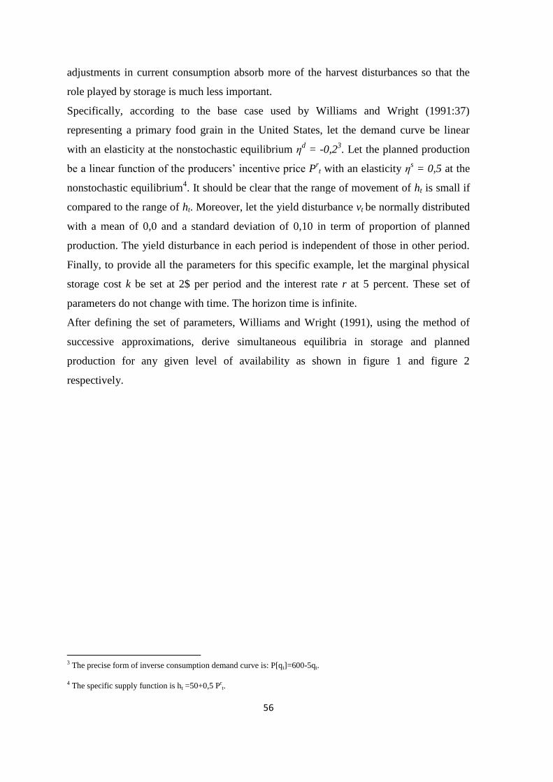
56
adjustments in current consumption absorb more of the harvest disturbances so that the
role played by storage is much less important.
Specifically, according to the base case used by Williams and Wright (1991:37)
representing a primary food grain in the United States, let the demand curve be linear
with an elasticity at the nonstochastic equilibrium ηd = -0,2
3. Let the planned production
be a linear function of the producers’ incentive price Prt with an elasticity η
s = 0,5 at the
nonstochastic equilibrium4. It should be clear that the range of movement of ht is small if
compared to the range of ht. Moreover, let the yield disturbance vt be normally distributed
with a mean of 0,0 and a standard deviation of 0,10 in term of proportion of planned
production. The yield disturbance in each period is independent of those in other period.
Finally, to provide all the parameters for this specific example, let the marginal physical
storage cost k be set at 2$ per period and the interest rate r at 5 percent. These set of
parameters do not change with time. The horizon time is infinite.
After defining the set of parameters, Williams and Wright (1991), using the method of
successive approximations, derive simultaneous equilibria in storage and planned
production for any given level of availability as shown in figure 1 and figure 2
respectively.
3 The precise form of inverse consumption demand curve is: P[qt]=600-5qt.
4 The specific supply function is ht =50+0,5 Prt.

57
Figure 2.1: Equilibrium storage as function of current availability
Source: Williams and Wright (1991:38)
In essence, in figure 1, for any value of current availability At, which includes the current
harvest ht and the carring St-1, thanks to the storage rule (11) it is possible to obtain the
corresponding equilibrium carryout St. Because the kink point A*, the storage rule in
figure 1 has an evident nonlinearity behaviour. Obviously, the specific current availability
corresponding to an exact positive storage depends on the specific parameters, but all the
storage rules has a kink point of discontinuity. In our example, according to the set of
parameters chosen, the kink point A* is 99.62 units according to Williams and Wright
(1991).
Another important characteristic of the storage rule plotted in figure 1 is the smooth
relationship between availability and storage over the kink point A*. The slope of this
relationship represents the marginal propensity to store for each current availability. The
storage rule is a line below the 45° over the kink point. It means that equilibrium storage
is not a perfect linear function of current availability or, in other words, as higher is the
availability as lower is the increased quantity stored.
Availability (At)
100 120
0
A*
20
0
Storage (St)

58
2.5 The effects of storage on planned production
In a setting with storage, in any period producers and storers allocate collectively the
current availability At between the aggregate consumption qt and the current storage St. At
the same time the amount being planted for harvesting in period t +1 (ħt+1) is setting.
Fixed point solution must be found together for St and ħt+1.
In the previous paragraph we have already seen the storage rule that tells us how much is
stored collectively for any given circumstances as function of the current availability At.
On the supply side there is an associated planned production rule which is the reduced
form equation giving a unique amount planted to be harvested the next period for each
value of current availability:
1 [ ]t tf A (12)
It should be clear that ħt+1 is in equilibrium with St , because St refers to the carryout from
the period t and the carryin for the period t +1. Both ħt+1 and St are committed in period t.
In essence, the reduced form equation for storage (11) and for planned production (12)
are simultaneously determined. Note that f s and f
ħ are different function, of course.
Figure 2 plots the equilibrium planned production as a function of the current availability
(12) deduced through numerical methods for the same group of parameters used for the
figure 1.

59
Figure 2.2: Equilibrium planned production as a function of current availability
Source: Williams and Wright (1991:38)
Like figure 1, the rule for planned production as a function of current availability has a
discontinuity at the same point A*. According to the figure 2, planned production ħt+1 is at
least 103.34 units for any availability below the kink point A*. This is the maximum
planned production which represents the level of planned production whenever storage is
zero. Moreover, when the availability is below A* the next period’s market is
disconnected from the current period’s market because the carryout is zero. On the other
side, when current availability is such that the equilibrium storage is positive (any value
over A*), the value of the exact availability affects the planned production. Generally
speaking, the higher is the carryout’s level, the lower will be the price. For these reason,
as shown in figure 2, to the right of A*, the marginal propensity to plan is negative, it
means that the slope is downward. Although storage is generally considered as a tool for
market stabilising mechanism, it clearly destabilizes planned production. In other words,
rather than a means of stabilizing production, competitive storage should be thought as a
substitute for production. In fact, when le level of current availability is higher and the
price of the commodity is low it should be more convenient, under the economic point of
view, to deliver supplies next period by increasing storage and reducing production. On
the other hand, if current availability is expensive, production is relatively more
Availability (At)
100 120
0
A*
0
Planned
production
for the
following
period ħt+1
90
100
0
hN

60
attractive. However, the combined action of storage and planned production makes
consumption more stable.
In both figure 1 and 2, the kick point A* does not denote an equilibrium value but marks
an important transition in the shapes of the reduced-form equations. In particular, below
the value of A*, the equilibrium storage is zero regardless of At, since a negative amount
cannot be stored. Moreover, all values for St and ħt+1 represent equilibrium values for the
corresponding At’s.
From the two reduced-form equations plotted in the figures, which denote storage and
equilibrium planned production respectively, can be derived the related reduced-form
equations for the other endogenous variables as function of At.
2.6 The effects of storage on market demand
Under profit-maximising storage, current price can be expressed as a function of the
amount in store. Using the inverse consumption demand (4), the identity (5) and the
storage rule (11) it is possible to obtain the inverse demand function for storage. Using
Wright and Williams notation (1982):
1[ ( ) ] ( )t t t tP P f S S S (14)
Where:
-Φ(St) denotes the current price corresponding to each quantity in store.
Williams and Wright (1991:39) define Φ(St) as “the inverse derived demand for the input
of the commodity into the storage production”. The problem in this approach is that the
demand curve for inventories as function of current price is not a true structural equation
such as the supply and consumption demand curves because its endogenous nature.
When the current price exceeds P*, expected future price net of all storage costs is less
than current price, so that there is no profit in storage.
The figure below puts together the storage demand function to the consumption demand
curve, which is also a function of the current price, obtaining the market demand
function.

61
Figure 2.3: Market demand with storage
Source: Williams and Wright (1991:38)
At the price P* the elasticity of market demand increases. This increasing in consumption
demand below P* by the storage demand function shows that the demand curve with
storage is highly non linear, being much less elastic at high prices. It means that a small
change in availability deeply affects the price. On the contrary, to the right of A*, small
change in availability does not change price considerably.
In figure 3, moreover, for any given availability is possible to determine the
corresponding spot price but also the breakdown of availability between consumption and
storage. For example, let be At = 110. The corresponding Pt is $93.12 along the market
demand curve. On the other side, along the horizontal line at that price, according to the
consumption demand curve, qt = 101.38 units, which implies that, in the same period, St =
8.62 units (110-101,38).
The same figure 3 has been used by Carter et al. (2011) stressing and explaining in a
better way the storage’s role in buffering price spike. In figure n. 4, in any given period,
total demand for the commodity equals the horizontal sum of the inventory demand curve
and the demand for current use as we have already said. When speculative inventories are
positive, the level of stock is high, total demand is relatively elastic since the market can
respond to adverse shocks by reducing inventories and improving the supply. On the
opposite side, when the level of stocks is low or even zero, total demand is relatively
Price (Pt)
100
Availability (At)
Market demand curve
Consumption demand curve
A*
100 120
P* PN
150$
qt
Consumption and market demand

62
inelastic because there is little capacity to buffer the gap between demand and supply with
the storage and also a small negative supply shock can determine a large price spike.
Figure 2.4: The Market demand function
Source: Carter et al. (2011)
2.7 Sequential equilibria in the system
So far, only a single equilibrium example has been considered. How the equations
interact through the time is not so easy as the single equilibrium example.
Next paragraphs illustrate, through numerical results, the interactions in the system
considering a time of eleven periods. It should be kept in mind that, for each period, the
weather is drawn from a random number generator. The weather sequence is plotted in
figure 4(a). In our example, given by Williams and Wright (1991: 41), over these eleven
periods the weather is quite bad most of the time reducing the realized production
compared to the planned production as it will be seen later. However, the system is not
affected by the number of time periods included. It means that, provided the situation in

63
the first period (A0), the sequence of weather condition, the set of parameters seen above,
the series of planned production, price and storage are time invariant. In other words they
would have been evolved in the same way starting in period 1162 or period 173.
For the sake of simplicity the first period of the sequence is called period 0.
Figure 4(b) illustrates the availability during the sequence of period starting from period
0. At the beginning the current availability is A0 = 97.73 units because the weather was
poor and the carrying small. This value of A0 is below the kink point A*= 99,62 units,
below which the equilibrium storage is zero as it has been seen in figure 1. For this reason
the equilibrium S0, shown in figure 4(c) is zero. It means that all the current availability
A0 is consumed. At the same time, the equilibrium planned production ħ1, plotted in figure
4(e), is 103.35 units. This value of ħ1 can be derived from the relationship between
equilibrium planned production and current availability illustrated in figure 2. Finally,
figure 4(d) shows the equilibrium spot price in period 0, P0 = $111.35.
In period 1 the weather turns out to be a little better than in period 0 but still under
average as it can be seen in figure 4(a). The realized harvest h1, because the weather
condition, is 101.44 units, quite different from the expected harvest ħ1 of 103.35 units.
Since in period 0 there S0 = 0, it means that there is no carrying from period 0 to period 1,
the A1 equals the realized harvest h1 = 101.44. From the reduced form equations for
storage and planned production through the current availability A1 the new equilibrium
can be defined. In fact, the equilibrium carryout S1 is 1.45 units according to the figure 1,
while according to figure 2 the equilibrium planned production ħ2 for the period 2 is
102.59 units. The difference between A1 and S1 shows the current consumption q1 = 99.99
units. If the full availability A1 = 101.44 were consumed, P1 would be $92.80 but, since
only 99.99 units are consumed during period 1, P1 = $100.05. In this way it seems that
storage supports the price or, in a different perspective, because of storage, price alone
does not absorb the exogenous shocks due to the weather condition. The availability in
period 2 is close to the availability in period 1. However, in period 2 some carrying from
the previous period (S1 =1.44 units) should be added to the realized production. The
quantity stored in period 2, S2, is 1.81 units that is the carryout for the period 3.
Unfortunately for the storers in period 3 the weather turn out in a better way. For this
reason, the price at which the storers sell their carryin in period 3 ($95.59) is below the
price ($99.66) at which they would have sold in period 2. This lost of value does not
indicate irrationality or a market failure. Storers cannot forecast the exact weather in

64
advance. Thus, the decision in period 2 was rational although not convenient under the
strictly economic point of view.
Period 4 is a good point to talk about because it represents the biggest positive yield
disturbance in the eleven period sequence. Because this extraordinary good weather in
period 4, A4 is 118.80 units as result. The reduced form equation indicates storage of
16.24 units corresponding for this availability. If our crop were not storable, it would
been consumed in period 4. The possibility to store spreads the disturbance over several
periods so that consumption in each of those later periods is slightly higher than
otherwise. In fact, both q5 and q6 (calculated form P5 and P6) are above 100 units.
A reduction in planned production is another way to absorb the shock caused by the
exceptionally good weather in period 4. In fact, the equilibrium planned production is
now 96.32 units that is lower than the same value calculated during all the previous
periods.
In period 4 it is clear how storage and planned production together absorb much of the
shock caused by the weather variance though moving in opposite direction.
Period 4 shows us how high storage occurs when prices are low and, on the opposite side,
low inventories occur when prices are high. It follows that expected price is decreasing in
stocks for positive levels of stocks but both these variables are endogenous variable that
are affected by the exogenous shock in supply and in demand. However, on the supply
side, the variability in the harvest is endogenous. Although the proportional deviation in
yields is exogenous, the planned production is a decision variable within the system.
Period 8 is an example of a very poor weather. The current availability in period 8 (A8) is
quite poor because the realized production is lower than the expected production but also
because the stored quantity from period 7 is not enough to cover the low realized
production. Again, the bad harvest could not have been forecast. Since, storage is costly,
it makes no sense to store for the rare poor harvest. In period 8 it is clear how the current
availability is just a function of past decisions, specifically storage and planned
production making the availability a predetermined variable rather than a true exogenous
variable. However, when the harvest is poor and the carryout zero, the link between
current availability and previous decision about planned production and storage is
essentially broken. The current availability during period 9 is not a function of the
carryin. In this way period 8 is just like the starting period 0. In both period 0 and period

65
8 current decisions are solely functions of current availability A0 and A8. A new
accumulation of a stockpile will be done in periods 9 and 10.
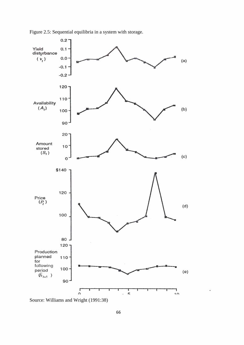
66
Figure 2.5: Sequential equilibria in a system with storage.
Source: Williams and Wright (1991:38)

67
If the number of periods is 1000 instead of 100, these patterns will be almost the same
and even more evident. In essence, as the number of periods increase, the frequency
distributions of the endogenous variables converge to stable distributions. These stable
frequency distribution are probability distributions. The joint probability distribution for
the various endogenous variables is distinct for each set of parameters.
To summarize, the sequential competitive equilibria can be described thought three key
behavioural conditions.
Firstly, in each period farmers plant up to the point at which the marginal expected net
revenue from their next harvest equals their marginal planting costs.
Secondly, in each period storers fix the quantity stored equal to the point where the
difference between the current price and the rational expected price for the next period
covers interest rate and storage costs.
Finally, as we have already said, the assumption that storage cannot be negative must
hold in any period.
The specific probability distributions for the endogenous variables reflect the properties
of storage over an infinite number of periods. It means that the realized price in period
t+250 will depend on the weather and the reaction by storage and planned production
over all those 250 periods. The probability distribution for Pt+250 is well defined since the
system is not explosive and any influence of particular circumstances in previous period
have been disappeared. Thus, the probability distribution for Pt+250 is the distribution
derived from an infinitely long time series.
Obviously, to generate an infinitely long time series is an hard task. However, Williams
and Wright (1991) simulated a probability distribution for 250.000 periods. The value,
period by period, for variables such as price were recorded. Figure 5 shows the invariant
long-run distribution for price and availability along with the market demand curve.

68
Figure 2.6: Probability distribution of availability and price.
Source: Williams and Wright (1991:38)
In the fourth quadrant is represented the probability distribution of the amount available
due to the sum of carryin and new virgin production. Thought the market demand curve
in the first quadrant, derives the probability distribution for price that is shown in the
second quadrant.
Figure 5 shows also the probability distributions of price and availability without storage
as dotted curves. The differences between the distributions with and without storage is
particular useful to better understand the role of storage in commodity markets.
Firstly, as regards the means, for this set of parameters, mean price with storage is higher
than mean price without storage. More in details, as well described by Wright and
Williams (1982:603), “storage causes a large asymmetry and possibly counter-intuitive
change in the distribution of price. Although the production disturbance is symmetric, the

69
distribution of price is not, because of the non-linearity of the constant elasticity demand
curve.” Thus, the effects of storage on the price distribution are asymmetric in a fashion
that storage is much more dependable in precluding commodity gluts and low price
instead that commodity shortage and high prices.
Secondly, the variance in a system with storage is lower than a system without storage. It
means that storage stabilizes the price reducing the frequency of both very high prices and
very low price. Finally, as can been in figure n. 5, storage makes the distribution highly
skewed with the long tail toward high prices.
2.8 Challenging the basic storage model
According to Stigler (2011:30), one the most important characteristics of price series is its
persistence defined as “its degree of autocorrelation” that shows “how past changes will
influence the course of future changes.” Typically, in price series with high persistence,
past shocks continue to persist influencing the commodity’s future price trajectory. In
other words, in the case of low autocorrelation coefficients, shocks effects dissipate
rapidly. By contrast, for series with high persistence, with a coefficient of autocorrelation
neat to 1, the same shocks have a deeper effect and require many more periods to return
to its normal trajectory. In the case of autocorrelation coefficient of 1, the same shocks
have a permanent effect and the series show an infinite memory.
In this last case the series is said to be non-stationary or containing an unit root which
means that its mean and variance will change over time. Alternatively, a time series with
an autocorrelation less than 1 is said to be stationary having a fixed mean and variance.
The concept of stationary in time series is well described in a formal way by Stock and
Watson (2003:447).
In essence, the degree of persistence impacts not only the variability but also the
predictability. As explained by Stigler (2011:30) “series with a coefficient lower than 1
exhibit stable forecast intervals, while series with a coefficient of 1 show forecast
intervals that expand over time. This means that they are impossible to predict.”
Moreover, “the question of a series’ persistence is also relevant for modelling strategy, as
non-stationary variables require non-standard statistical techniques”.

70
The basic storage model in presence of an independent and identically distributed (i.i.d)
supply and deterministic demand function, induces high price autocorrelation but still
stationary. The model, also shows a skewed distribution of commodity prices even under
symmetric supply and demand shocks. Moreover, time series of prices will show isolated
spikes “a feature determined by the possibility of occurrence of stockouts that are periods
in which stocks fall to zero. Storage, in fact, introduces a key nonlinearity in the market
demand, implying two different regimes of price volatility, one in which abundant
reserves can buffer the effects of negative shocks in supply, and another in which, at high
prices, the low levels of stocks leave the market particularly vulnerable to shocks in
supply or demand” (Cafiero et al. 2011b:302).
A clear consensus about the empirical validity of the standard storage model is still under
debate,
Empirical tests of the storage model began with Deaton and Laroque (1992). In their
influential article they investigate how the storage model is compatible with the relative
high, but still stationary, auto-correlation found in annual price for a large number of
commodities. They were quite sure about the stationary hypothesis concluding that
random walk (non-stationary) in price series “seems very implausible, at least for
commodities where the weather plays a major role in price fluctuations.” (Deaton and
Laroque, 1992:31). In order to achieve these results, the authors used a so called
Generalized Method of Moments (GMM) estimator showing that the prices dynamic
analyzed are consistent with a two regime autoregressive process in which price at the
time t is correlated to the previous one only if the latter is below a given threshold due to
the storage. This result was encouraging but was not a definite evidence in support of the
validity of storage model given that other model of price behaviour could generate the
two-regime auto-regression. As well observed by Cafiero et al. (2011b), Deaton and
Laroque (1992) used a limited range of parameters values for the fundamental parameters
of the model opening the question of whether there are other values for the fundamental
parameters of the model that could generate high levels of serial correlation like those
observed in the series of actual prices, A few years later, Deaton and Laroque (1995,
1996) challenged the storage model introducing the Pseudo Maximum Likelihood (PML)
empirical estimation approach in order to estimate the parameters of the underlining
demand and storage cost relation. In this case, they could not confirm the positive results
obtained in 1992 with the GMM estimation, and found that, in order to replicate the

71
observed levels of autocorrelation in their model, it was necessary to relax the assumption
of i.i.d harvest. This conclusion is well summarized in Deaton and Laroque (2003:2):
“The speculative model, although capable of introducing some autocorrelation into an
otherwise i.i.d. process, appears to be incapable of generating the high degree of serial
correlation of most commodity prices.” In particular, in Deaton and Laroque (1992) the
price autocorrelation was far below the sample autocorrelation observed. Moreover, the
specification of their model did not generate sufficient price variation in comparison to
the values observed for most of commodities analysed.
However, according to Cafiero et al. (2011b), the negative results of the PML estimation
should be attributed to the particular specification adopted by Deaton and Laroque (1992)
model instead of the validity of the speculative storage model as a whole.
Cafiero et al. (2011a) found that after a small modification of Deaton and Laroque’s
approach, the storage model was indeed able to replicate high-correlations re-establishing
the empirical relevance of the standard storage model. In fact, the consumption demand
function specified by Deaton and Laroque (1992) with price elasticity within the range -
0.5 to 0.1, is more sensitive to price than are consumption demands in the major
commodity markets. In order to increase the price variation in the model, Cafiero et al.
(2011a) used a reduced and more reasonable price elasticity demand in the range between
-0.2 to -0.067. Moreover, the same authors assumed no storage cost other than interst
charges in order to favour high serial correlation. In this way, the authors demonstrate
how to use the estimated model to generate distributions of the price next period, given
the past history of prices and conditional on the amount of stocks implied by the current
price. This estimations seem to be very useful in anticipating periods of high price
volatility and in planning policies to avoid prices peak and crisis in food markets.

72
3. INTERNATIONAL WHEAT MARKET: A THEORETICAL
FRAMEWORK
Price market determination for wheat has been deeply discussed by producers, consumers
as well as policy makers since long time. A large strand of literature has been involved in
attempting to understand the wheat price formation mechanism in world market. Wheat
world trade has changed in a massive way since the 60’s. According to Sarris (2000),
world trade has become more liberalized thank to several international agreements and to
the role of governments in cereal markets that have strongly reduced their interventions.
Moreover, different major producing countries such as China and Russia are undergoing
significant economic changes increasing their income pro capita and, in its turn, their
eating habits. Technological changes in production and new communication tools have
further changed the market framework increasing the integration of regional markets.
The purpose of this chapter is to explore the price formation mechanisms of world wheat
market. Firstly, different theoretical models discussed since the 60’s in order to provide a
theoretical framework for analysing wheat price behaviour will be briefly introduced.
Secondly, a recent annual model for United States wheat price firm used by USDA in
short-term market analysis and long term base line projection will be deeply explained.
3.1 Price formation in world wheat market. A theoretical review
Wheat international market has been deeply analysed and several theoretical models have
been proposed to formalize the price formation mechanisms. McCalla (1966) attempted
with his pioneering paper to present a formal model about international wheat market
during the 1950s and 60s. The author defined a cooperative duopoly model where Canada
and the United States are the duopolists, with Canada the price leader and the United
States the usually silent partner adjusting price within a zone of cooperation. All the other
exporters and big producers such as Australia, Argentina and France create a large group
constituting a “fringe of price follower” setting a price just below the price set by
duopolists to clear their stocks. According to McCalla (1966), the duopoly approach was
the better approach to describe the market structure at that time at least for two reasons.
First of all, Canada and United States controlled 60% of the market. Second, market
power shows a strong correlation with the ability to hold stocks. These two countries had

73
adequate storage facilities to permit holding in comparison with the other exporters giving
them a great market power.
Both countries had the objective to maximize exports subject to the implied duopoly
relationship. The market structure results in a deterministic solution for price and exports.
However, Canada and United States’ demand function was the residual from the
aggregate demand and supply function of the smaller exporters.
Furthermore, McCalla (1966) recognized the possibility that changes in international
conditions may alter the structure of world wheat market underlining the inherently
instability of international trade in wheat due to domestic agricultural policies. The author
argued that rapid increases in Australian wheat production with a strong declining stock
of the United States and Canada may bring a severe change in the market structure.
In line with these findings, ten years later, Alouze, Watson and Sturges (1978) postulated
a triopoly model of world wheat market between United States, Canada and Australia
with Canada as a revenue-maximizing price leader. This model was supported by three
pieces of evidences well explained by Wilson (1986).
Firstly, Australia’s wheat stocks were increased since the end of the 60’s. In this way
Australia reached a higher market power. Secondly, Australia domestic agricultural
policy was completely changed in term of stocks supply. In fact, especially during the end
of the 60’s, Australia did not clear its stock in each marketing year. Finally, meetings
organized by Canada and United States to define price and market shares started to
include Australia too.
However, during the 1970’s, the triopoly was no longer able to represent the market
structure for a number of reasons. New conditions changed the framework. First of all,
large purchase by Russia greatly reduced the large surplus of the previous decade. Since
market power was strictly correlated with stockholding, the decreased level of stocks
create a competition to set price and exports between the major exporters.
Moreover, the models described so far don’t recognize the potential substitutability of
wheat by class and origin but, for the sake of simplicity, assumed them to be
homogenous. Conversely, Oleson (1979) has been the first to take into account the
importance of wheat quality and the role of different classes and origin in maintenance of
market power. In essence, he distinguished three historical periods to describe wheat trade
framework. During the first one, from 1953 to 1962, Canada is the market leader because
its dominance in the high protein wheat market. The United Stated had, in that period, a

74
limited supply of higher protein wheat but larger supply of other classes. For this reasons,
United Stated accepted Canada’s price leadership for the high protein wheat market
establishing export prices only for other classes. Fringe competitors, in line with
McCalla’s (1966) results, had limited storage for all wheat classes and followed a policy
of minimizing stocks each market year.
From 1963 to 1972, the second period, the role of Canada as price leader was not so
strong anymore. United States and Australia, in a lesser way, increased their production
of higher protein wheat. Moreover, new technology in the baking industry resulted in
reduced demand for higher protein wheat. All this factor lead to an eroded Canada market
power.
After 1972, the last period, United State become the recognized price leader. According
to Oleson (1979) several factors contributed to this transition. Firstly, there was a severe
expansion in export demand especially form URSS. This strong demand was mostly
covered by the US. Secondly, the strong interaction between US and Canada in defining
prices and exports was suspended. In other words, US adopted an open-market pricing
policy subject to the operation of government price interventions such as loan rates5,
target prices, supply control and storage payments. Finally, Canada exports, during this
period, were influenced by logistics and transportation problems which served as a
constrain and affected their storage policy. All these aspects led Canada to become a new
member of the large group of smaller exporters that is called by McCalla (1966)
“competitive fringe”.
Considering this changed international wheat market framework, Wilson (1986)
described wheat international market using a price leadership model with the US being
the price leader. According to the author, “US farm programs, particularly the loan rate
program, play a dominant role in the international price structure for wheat. It is the
interaction between cash and futures markets with the loan program which determine
international prices, which are effectively ceiling prices for the price taking competitive
5 “The loan rate is the price at which farmers can borrow from the government against their crop. If crop
prices rise, the farmers can redeem their crop and sell it to repay the loan. If prices do not rise, the crop is
retained by the government as full payment of the loan. In many years, the US loan rate becomes a price
floor, which supports the US market price and because of the size of US exports the world price as well”.
(Mitchell and Duncan 1987:20)

75
fringe. It is in this indirect way that the US has assumed the role of price leader, although
it was probably not intentional.” (Wilson 1986:29).
In essence, the main features of Wilson’s dominant country price model can be
summarized in this way: US is assumed to be the price leader and all the other exporters
are included in a large group of competitive fringe. Obviously, they are considered price
takers since they are individually too small to affect international price. Moreover they
are thought to act independently each other.
The supply function for the competitive fringe taken as a whole has a great influence in
demand function for the US. In particular, the elasticity of US demand function is
affected by the elasticity of the supply function for the competitive fringe. “A more
elastic competitive fringe supply implies a more elastic effective US demand” (Wilson
1986:30). For instance, the author suggests that technological improvements and
increased exporting capacity by smaller exporters, result in lower export provided by US.
In other words, with prices fixed by US, changes in aggregate demand are all absorbed by
the US in terms of stock and supply adjustment. Wilson (1986) noted also that an
appreciation of the US dollar negatively affects the effective demand function for US
increasing exports from competitive fringe. Finally, this price leadership model was
supported also by the export strategies adopted by the smaller exporters. The author noted
that France, Argentina and Australia adopted policy to minimize the level of stocks
cleaning the market each year with price that were in line with US price or even below
US price. Canada is presented as a special case. This country was used to maintain high
stock level during the 60’s reaching a great market power. Its stock level became less and
less until the 80’s. This decreased level of stock in addition to increased exports
represents a clear political choose that “reflect a recognition of reduction of market
power.” (Wilson 1986:30)
In spite of Wilson’s model, Mitchell and Duncan (1987) proposed a model that is
generally consistent with the dominant-firm oligopoly model for analysing the behaviour
of the major grain exporters. Their results, however, showed that rice and coarse grain
markets were very closely to the oligopoly model with the United States being the
dominant firm. The same results for wheat market were a little bit different. In this case
there was not a clear market leader. Wheat market can be better defined as a more
complex oligopoly involving a shared dominance between the United States, Canada and
Australia. Moreover, in line with the conclusions of Alouze et al. (1978), price leadership

76
is provided by the United States through its wheat loan rate. In essence, as well described
by Mitchell and Duncan (1987:3) United States with Canada and Australia represent the
word’s residual supplier for wheat. United States, because its loan rate, has established
price floor for wheat and allows other small exporters to sell as much wheat as they
choose at that price. For this reason, the behaviour of the United States in wheat market
and, more generally, in grain market, has fundamental implication for all the small
exporters. “As long as the United States, or any other country, behaves like the price
leader, others can export at the price it sets.” This opportunity has been used in a
profitable way by Argentina for the wheat case.
According to the model, when world import demand decreases United States greatly
reduces its export supply while other small exporters are only little affected. This is
because the role of world residual supplier of the United States. The reduction in export is
reflected in an increased stock level. This behaviour, well explained by the model, is in
line with growing stock level of the United States and the remained low level of the other
exporters during the years analysed by Mitchell and Duncan (1987). Moreover, when the
United States dollar appreciated against other currencies it reflected immediately in
United State export. In fact, when US dollar appreciates compared to other currencies, the
price of wheat in international market is higher because it is usually expressed in US
dollar. Considering that United States acts as a residual supplier in the model and because
its price floor is not changed according to the US exchange rate, it should be clear that the
import response to the dollar appreciation result only in a severe loss in export by the
United States. Obviously, opposite results are reached in the case of US dollar
devaluation.
Since mid-1980’s market conditions and prices for wheat have been deeply changed.
Agricultural sector has become more market oriented under agricultural policy changes of
the last 30 years.
A useful and relatively recent price determination model for wheat implemented by
Westcott and Hoffman of US Department of Agricultural (1999) provides a complete
analytical framework for short term market analysis and long term baseline projections.
In essence the model takes into account mainly to types of factors that influence prices
such as market supply and demand aspects and government policy variables. The model
is augmented by variables that reflect the changing role of agricultural policies,
international market conditions and, finally, the role of wheat feeding and competition

77
with corn for feed use. In the next paragraph USDA model price determination will be
discussed more in detail.
3.2 USDA wheat price determination model
Because its simple structure and its small data requirement, USDA wheat price
determination model is largely used in price forecasting and market analysis of supply
and demand condition. The model simply uses four sources of information. Firstly, a
stock to use ratio parameter to take into account the effects of market supply and demand
factors on price determination. Secondly, Government agricultural policies that may
directly affect price definition are included in the model. Then, international market
conditions are also analysed since the market structure for wheat is considered much
more competitive than in past decades. Finally, the role of wheat feeding and competition
with corn for feed use is assumed affects the price determination mechanism. Westcott
and Hoffman (1999:21) present model performances measures showing that the price
model reflect actual prices very well and that “the statistical measures indicate good
performance for the price model and suggest that price model provides an analytical
framework that can be useful in price-forecasting application”. The authors also state that
“most differences between the model estimates and the actual prices are less than 20 cents
per bushel of wheat.” In next paragraphs each variables included in the model will be
briefly described.
3.2.1 Supply and demand factors affecting wheat price
The effects of market supply and demand factors on price determination represent the
main core of the model. The components of supply and demand will be briefly considered
separately.
Wheat supply includes beginning stocks, imports and production. Wheat is produced
annually and under modest conditions it is storable for long period of time. Carryover
stocks from the previous year become the beginning stocks for the current year increasing
the current production. We have already seen how large stocks can provide an additional
source of supply in a low production year buffering prices spike. In order to improve
wheat supply each country may acquire wheat from the international markets. Generally

78
speaking, imports market is quite competitive involving a large number of countries
which are not big enough in terms of purchases to affect the international price. In
particular, focusing on US, wheat imports have been insignificant relative to the total
supply. Finally, production can be defined the major component of supply at least for the
countries that are taken into consideration in this thesis. Production depends on the
amount of acreage harvested and the yield per surface unit. Acreage planted “reflects
producer net returns per acre for a given commodity compared with returns for competing
crops” (Westcott and Hoffman, 1999:3). Government policy such as subsidies and
agronomic consideration can severely alter net returns per acre affecting planting
programs. Yields is affected by a plethora of factors including climatic conditions, farm
management and also wheat variety and soil quality. Unfortunately, because weather
condition, in any year yields can be pushed above or below trends affecting in this way
international price.
On the demand side, major components for wheat include food, seed and industrial use,
feed and residual, exports and, finally, carryover stocks.
Generally; food, seed and industrial use is the largest component of wheat total domestic
demand. Within this category, consumption for food usage is the greater component.
Human consumption is close related to population growth and income level. Moreover,
food uses are inelastic to farm-level prices since the farm value of wheat in consumer
food stuff is relatively small.
Feed use for wheat is much less important than for corn that is the main feed crop. Feed
use is more variable than food use because this kind of use is strictly related to wheat
price compared to corn price and wheat quality. Usually, most feed use of wheat occurs in
the summer, when wheat prices are seasonally low following the wheat harvest but before
corn is harvested.
Export is an important component in wheat total demand for the countries included in this
thesis. We have already introduced different models explaining demand exports for the
main exporters countries. In those models, international trade in wheat has evolved from
an oligopoly in which Canada was the price leader (McCalla, 1966) to a price leadership
model in which the US is the price leader (Wilson, 1986). More recently, Westcott and
Hoffman (1999:7) recognises that although the US is the largest world exporter of wheat
its world market share is not enough to be considered a price leader having a less
dominant role in international market with respect to earlier years.

79
Market conditions of supply and demand are summarized in the stock to use ratio. This
measure is defined as “stocks of the commodity at the end of a particular time period
divided by use of the commodity during the same period of time” (Westcott and
Hoffman, 1999:11). Stock to use ratio has been largely used in many models to represents
supply and demand characteristics in an annual framework (see for instance Van Meir,
1983; Baker and Menzie, 1988). In line with these previous models, Westcott and
Hoffman (1999) used stock to use ratio measure but in a quarterly framework.
This measure, in line with previous findings and literature, is negatively related to prices
and provides a downward sloping nonlinear curve of prices plotted against ending stocks
to use ratios.
3.2.2 Agricultural policies affecting wheat price
Beyond supply and demand factors, Government programs are considered important in
affecting price determination mechanisms for this reason government policies variables
are included in the model. There is a plethora of agricultural policies that may affect
supply, demand and pricing of wheat directly and indirectly. Generally, policies affecting
supply and demand factors have an indirect effect on wheat prices such as acreage
reduction and set aside programs on the supply side and export subsidies on the demand
side. Price effects of these policies are usually already included in supply and demand
data and for this reason do not need to be considered again.
Government price support and commodities storage programs affect in a more direct way
wheat market price beyond the effects on supply and demand. These programs should be
considered in a more serious way and included in the model.
More in detail, price support programs for wheat have been popular in US. The loan rate
is the most popular instrument of price support in US. If market price is below the loan
rate it would be better for the farmer, under the economic point of view, defaulting on the
loan and keeping the higher loan rate. According to Westcott and Hoffman (1999), loan
rates for wheat increased in the late 1970’s and remained relatively high until the mid-
1980’s. In 1986’s price support program started to change reducing significantly the
effect of price supports on the market price. In essence, the loan rate continued to be used
but it no longer supported price being well below market price in most of the recent years.
These changes are considered as a part of a general movement in US agricultural policy
toward a more market orientation.

80
A similar evolution can be observed in commodities storage programs in which
government programs led to a large build up of stocks in the early 1970’s to the mid-
1980’s.
The major storage programs were the Farmer-Owned Reserve (FOR), the Commodity
Credit Corporation (CCC) and finally, the Food Security Wheat Reserve (FSWR).
More in details, Commodity Credit Corporation (CCC) can be defined as public stocks
owned by the Government acquired by loan defaults or market purchases. These stocks
have severely affected market price because they have generally not been readily
accessible to the marketplace.
The Food Security Wheat Reserve (FSWR) was created at the beginning of 1980’s with
the aim to provide a government wheat reserve of up to 4 million metric tons for
emergency food in developing countries.
However, also for these programs, between 1985 and 1990, deeply changes in the
legislation toward market oriented stockholding policies reduced wheat stocks level and
the impact of these programs on wheat price.
In conclusion, policy changes since 1986 until recent have continued to reduce price
effects of government price support and commodity storage programs. As a consequence,
price for wheat has been mostly determined by market supply and demand factors with a
reduced influence of government policies.
3.2.3 The pricing model
The pricing model described by Westcott and Hoffman (1999) relates wheat price to
ending stocks. In particular, in its simplest form, stocks are a function of price. The
equilibrium condition to clear the market determines the price at which supply equals
demand plus stocks. In a more formal way, using Westcott and Hoffman (1999:12)
notations we have:
t-1S=f(p ,z) (Supply_function) (1)
1D=g(p,p , )t z (Demand function) (2)
K=h(p,z) (Stocks function) (3)
S-D-K=0 (Equilibrium condition) (4)

81
In which, S is supply, D is the demand, K is the ending stocks, p is the market price and z
is a set of exogenous variables. Lagged prices are included in both supply and demand
function. They are particular important for wheat used for feed since livestock production
decisions made in previous periods in response to prices in those period affect feed
demand over a number of years in advance. Export demand is also considered function of
lagged prices to reflect international supply response. Supply is positively related to
expected price while, on the other hand, demand and stocks are negatively related to
price.
In equilibrium price can be derived from the inverse of the stocks function. In a more
formal way it can be written as follow:
-1p=h (K,z) (Price equation, inverse stocks function) (5)
Equation (5) represents the basic pricing model. However, adjustments are needed to take
into account other factors affecting prices. In particular, adjustments will be added to
include Government programs that directly affect price determination such as
Government loan program and stockholding policies. Other adjustments will introduce
variables related to global wheat market factors and wheat feed use and related cross
commodity pricing considerations. These adjustments result in upward or downward
shifts of the basic functional relationship between ending stocks and prices expressed by
equation (5).
Starting from the different effects that government programs have on price determination
two additional terms are added in equation (5).
LR= the effect of Loan rate program;
CCC= the effect of Government programs.
In essence, there is a negative relationship between prices and total stocks as we have
already seen. However, we should consider separately the effect of the total ending stocks
from the effect of the government owned stocks on price determination mechanism. For
the former, larger total stocks are generally associated with lower wheat price. For the
latter, larger Government owned stocks lead to higher price. This is because Government
stocks are much more isolated from the marketplace.
In order to keep into consideration the role of global wheat market in price determination,
a variable reflecting the world wheat market structure should be added to the basic model.
In fact, although the United States is the largest exporter, its role is not as dominant as in
the corn market at least during the last decades. US wheat price (and, in its turn, world

82
wheat price since it is strongly anchored to the US price) is affected by world market
conditions. A variable representing stockholding in four major exporters beyond US is
added to the pricing model to reflect this international market effect. Larger ending stocks
in EU, Canada, Australia and Argentina lead to lower wheat price in US. In line with
Westcott and Hoffman (1999) notation, a variable called C4K will be added to include
competitors stocks effect in price determination mechanism.
The last two adjustment to the basic model reflect the effect of wheat used for feed
purposes compared to total usage and cross commodity pricing considerations with
respect to corn.
In particular, wheat competes with feed grains especially during the summer when wheat
has been already harvested and all the other feed grains have not. Usually, if wheat is
largely used for feed, this lower value usage is reflected in a lower price. Moreover, as
well explained by Westcott and Hoffman (1999:13) “when low wheat prices lead to large
wheat feeding, typically in summer, the wheat price tends to be influenced by price of
competing feed grains such as corn.
To represent these two wheat pricing consideration, the two variables added to the basic
model are briefly described below:
FS/U: summer quarter wheat feed use expressed as a share of total use. This variable
should reflect the importance of wheat used as a feed in the season average price. In
essence, larger summer quarter wheat feeding means lower season average price.
PCS: Summer quarter corn price provides a measure of the level of cross-commodity
pricing influence provided from competing feed grains. In particular, “the higher the price
of corn in the summer, the higher the price of wheat used for feed, and thus the higher the
overall season average wheat price” (Westcott and Hoffman, 1999:13).
Adding these wheat price considerations to the general pricing model, the price equation
(5) for wheat can be written as follow:
-1p= h (K, CCC, LR, C4K, FS/U, PCS, z) (6)
The double log functional form is used to estimate equation (6). As we have already
explained, the coefficient on the stock to use ratio is negative because the negative
relationship between wheat price and stock to use ratio. Thus, this functional form
provides a downward-sloping, convex-shaped relationship between the stock to use
variable and wheat price. Most other explanatory variables used are also used in

83
logarithm from. Only the government owned stocks variable is not transformed to
logarithm.
USDA wheat price model specification is shown in equation (7) below:
Ln(p)=a + bLn(K/U) +c(CCC/U) + dLn(LR)Dum7885 + fLn(C4K/C4U) + gLn(FS/U) + hLn(PCS);
(7)
The variable p is the firm level price, LR is the wheat loan rate and K is the total stock. U
represents annual utilization of the crop. A dummy variable Dum7885 is added to
represent the effects of the loan program on wheat price from the late 1970’s to 1985.
During this period, wheat loan program had a major effect on price level. For this reason,
Dum7885 variable equals to 1 in 1978-85 and equals to 0 in other years.
CCC represents government owned stocks; C4K and C4U represent stock and use in the
main exporters (EU, Canada, Australia and Argentina); FS represents wheat feed use in
the summer quarter and PCS is the price for corn in the summer quarter.
The terms a, b, c, d, e , f, g and h are parameters to be estimated using ordinary least
squares regression.
The expected sign of the total stock to use ratio coefficient (b) is negative as we have
already seen. In spite of this, the coefficient (c) for the government owned stock to use
ratio is expected to be positive. This because larger government stocks at the end of the
year indicate that a greater share of the total stocks are not accessible to the market place
leading to higher price.
Price government programs summarized by the loan rate had a great positive influence on
wheat market price up to the middle 1980’s. The expected sign for the coefficient (d) is
positive when the dummy variable values 1. Previous models for wheat price
determination used a different specification for the loan rate. In particular, the dependant
variable was defined as the farm price minus loan rate. This is particular useful when
most part of the dataset is collected before 1985, when the effect of the loan rate was
particularly significant for the price determination. In contrast, Westcott and Hoffman
(1999:15) model uses a large number of data belonging to the period post 1985 when the
effect of the loan rate in affecting wheat price is no so important anymore. Thus,
according to the authors, “rather than including the loan rate in the dependent variable, it
seems more appropriate now to include the loan rate as a separate independent variable
for the years when high price supports affected prices, providing a policy shift effect on

84
price determination in those years. With this specification for the loan rate, the dependent
variable is the farm level price.”
The stock to use ratio for the major exporters beyond US is added in the pricing model to
account the effect on US wheat price of condition in international market. Obviously, a
larger competitor stock to use ratio results in lower international price, exerting
downward pressure on US price as well. Thus, the sign of the coefficient (f) is expected to
be negative.
Finally, some considerations about the value of the coefficients representing feed wheat
usage and cross grain pricing considerations.
The two variables used to represent the feed use effect on wheat prices are expected to
have opposite effects on wheat prices. In particular, summer quarter wheat feed use as a
share of total annual use is expected to have a negative effect on wheat farm price
(coefficient g is expected to be negative). On the other hand, the variable representing the
price for corn in the summer quarter is expected to have a positive effect on wheat price
(coefficient h should be positive).

85
4. WORLD WHEAT MARKET IN TERMS OF PRODUCTION,
CONSUMPTION AND TRADE
Price, consumption and stock in world wheat market have been a major concern for
private producers, consumers and, most of all, governments. The reason is that a market
failure leading to high price can lead, in its turn, to large income transfers between
various market participants. Obviously the poor people is the most vulnerable in front of
an increased wheat price and an augmented volatility of prices.
During the last decades, world wheat market has deeply changed under different point of
views. First of all, the market has became more liberalized and, on the other hand,
different governments have reduces their intervention in the in cereal market. Secondly,
several major producing countries such as China and Russia, are deeply changing under
the political and economic point of view. Finally, technological changes in production
and improving in communication tools are also factors affecting the world wheat market
(Sarris A.H. 2000).
At the present time, world wheat market is segmented into groups of countries with
different productive capacities and level of use. A small number of countries strongly
influence global wheat market producing and exporting a large portion of global wheat.
As it will be seen later, also the ending stocks of wheat in global markets appears
concentrated in few countries or regions. On the other hand, world wheat import market is
not so concentrated. In essence, the global wheat market is characterized by a small
number of wheat exporting and producing countries that sell to a relatively larger group
of importers. China and India represent a particular case. They are two major wheat
producing and usage countries but they are not so involved in trade focusing on the
domestic market. Given the critically important role of wheat as human food, seed and
industrial use, world wheat demand is projected to increase along with the world
population that is expected to grow in the next years. Nevertheless, the major role played
by some countries in definition of global wheat market supply-demand balance is unlikely
to change appreciably in the coming future.
The purpose of this chapter is to is to briefly present a complete picture of world wheat
market using data covering the last decades and introducing projection for the coming
five years.

86
Generally speaking there are different factors affecting global wheat market such as
supply of wheat in terms of production and stocks level, the demand of wheat in terms of
consumption for human food, feed and industry uses and finally export. Other factors,
that are less important but that should be keep in mind, are wheat quality, logistical costs
and political instability. According to these factors, global wheat market will be discussed
taking into account firstly the production side, than the consumption side and finally the
trade. The information provided represents a general overview and should not be
considered as a complete studies on world wheat market.
4.1 World wheat harvest Area
According to O’Brien (2011), the planted area of wheat in the world in the 2010/11
marketing year is estimated to be over 220 million hectares which is in line with the
average planted area since 1987/88 (218 million hectares).
The 10 largest wheat producing countries provided an average of 79,9% of world wheat
harvested acreage over the period 1987/88 to 2010/11 as showed in figure n. 4.1.
Figure 4.1: World wheat harvested Area
Source: O’Brien (2011), Agmanager.info article.
Considering the most recent period 2008/09 to 2010/11, the 5 more important countries in
terms of average world wheat harvested acreage covered more than 50% of world planted

87
area. In this period India is the country with the larger harvested acreage followed by
Russia and European Union (figure n. 4.2).
Figure 4.2: World wheat harvested acreage by Country average of 2008/09 to 2010/11
(1000 ha)
Source: O’Brien (2011), Agmanager.info article.
According to International Grain Council forecast, global harvested area are projected to
expand by around 0.4% annually with a slightly increased average yields until to 2016/17.
4.2 World wheat Yields
According to O’Brien (2011), the marketing year 2010/2011 was characterised by an
average world wheat yields of 2.90 metric tons per hectare. The same value calculated
since the 1987/88 marketing year has been estimated to be 2.67 mt/hectare that means an
average annual increase of 0.03 mt/ha over the last 24 year. Considering the wheat yields
by countries in details it should be noted the huge difference between regions. In
particular, the highest average yields over the last decade were registered in the European
Union (5.14 mt/ha) followed by China with 4.35 mt/ha with an impressive yields trending
upwards close to 0.12 mt/ha per year. Figure 4.3 summarizes the wheat yields over the 24
year period for the 10 largest producing countries.

88
Figure 4.3: world wheat yields by countries
Source: O’Brien (2011), Agmanager.info article.
4.3 World wheat production
According to the International Grain Council, world wheat production in the 2010/11
marketing year is close to 649 million of tons in line with O’Brien (2011) estimation.
Moreover, the same author provides an average world wheat production of 589 millions
of tons since the 1987/88 year with average increase of 5 millions of tons per year over
the 24 year period. The production of wheat is strongly concentrated in some countries. In
fact, the 10 largest wheat producing countries produced an average of 84.3% of world
wheat over the same 24 year period as showed in figure 4.4.

89
Figure 4.4: World wheat production by country
Source: O’Brien (2011), Agmanager.info article.
As showed in figure 4.4, some important countries such as Ukraine, Australia and Russia,
have a larger variability in wheat production compared to other countries. This is in line
with the value of the variability coefficient calculated by O’Brien (2011). The value of
the coefficient measures the historical variability in wheat production relative to the
average quantity produced since 1987/88. Ukraine, Australia and Russia have a
coefficient variability of 0.33, 0.30 and 0.22 respectively. On the other side, the same
coefficient for United States and European Union measures 0.12 and 0.09 respectively.
During the last 3 year period (2008/9 to 2010/11), the three largest countries in terms of
average world wheat production were the European Union, China and India that together
provided almost the 50% of the global wheat production followed by United States and
Russia (figure 4.5).

90
Figure 4.5: World wheat production by country 2008/09 to 2010/11 in metric tons
Source: O’Brien (2011), Agmanager.info article.
China is the second largest wheat producing countries after European Union.
Nevertheless, China produces mostly low quality winter wheat. This fact, in addition to
its increased demand, explain why they import mostly high quality wheat in order to
improve the nutritional level of their domestic wheat.
Finally, International Grain Council outlook forecasts a production record for 2016/17
close to 714 million tons due to an expanded harvested area and a slightly increase in
average yields.
4.4 World wheat utilization
World wheat total use in the 2010/11 marketing year is estimated by O’Brien (2011) to be
788,011,000 tons. This compares to average world wheat use of 735,475,000 tons since
the 1987/88 marketing year, with average increases of 6,397,000 tons per year over the 24
year period. Over the half of average world wheat usage during the 3 most recent
marketing years is concentrated in 4 regions; the European Union (19% of total usage),
China (14%), India (10%) and the United States (8%)

91
Figure 4.6: World wheat total use by country average of 200/2009 to 2010/2011 (1.000
tons)
Source: O’Brien (2011), Agmanager.info article.
FAO food outlook (2011) provides different and lower data for world wheat total
utilization estimating a total use over to 667 million tons for the 2010/11 marketing year,
20 million tons higher than the previous year. FAO forecasts an increase in total wheat
utilization for the next years mostly in response to larger availability and larger use of
wheat for animal feed because more competitive relative to maize. This is in line with the
International Grain council outlook which estimates an annual increase of 1,1% in
consumption reaching a total utilization close to 716 million tons in 2016/17.
In the next paragraphs, total wheat utilization will be described in function of the specific
usage of wheat for food, feed and other uses respectively.
In fact, FAO (2011) splits up the total utilization in food, feed and other usage estimating
a human food use for more than 70% of total usage (468 million tons). Feed use and other
use (including industrial use and seeds) accounting for 19% and 11% respectively.

92
4.4.1 World wheat food, seed and industrial use
According to O’Brien (2011), world wheat food, seed and industrial use in 2010/2011
marketing year is estimated to be 539 million tons. Since the period 1987/88, the average
of wheat total utilization is measured close to 504 million tons. This means that the total
utilization is increased with an average of 5 million tons for year over the 24 year period
as clearly showed by the figure 4.7.
Figure 4.7: World wheat food, seed and industrial use by country
Source: O’Brien (2011), Agmanager.info article.
China is the most important region in terms of wheat total utilization during the period
2008/09 to 2010/11 followed by India and European Union. This three countries or
regions use together an average of 50% of world wheat as well described by the figure
below.

93
Figure 4.8:World Wheat Food, Seed and Industrial Use by Country, average of 2008/09
to 2010/2011
Source: O’Brien (2011), Agmanager.info article.
More in details, direct human consumption is forecast to slightly increase driven by
expanding demand in developing countries. FAO (2011) estimates a 68 kg annual
consumption per person, which is in line with the level of the most recent years. It means
that the global food use of wheat is continuing to keep up with average world population
growth. China, that is one of the major consumer country, is forecast to show a slow
decline in per capita wheat consumption from the quantity of 73 kg at the beginning of
the millennium to a level of just 64 kg. This decline is mainly due to larger consume of
more value added food products in response to the income increase.
The combination of industrial use, seeds and losses in post harvest operations, account for
11% of world wheat production in 2010/11. The industrial use of wheat has slightly
increased during the past decade driven by larger utilization of wheat as feedstock and,
more recently, for biofuels production. According to the International Grain Council
(2011), total wheat industrial usage could reach 21 million of tons in 2011/2012 with an
increase in wheat used for biofuels production that will reach 7,3 million tons, 22%
higher than in 2010/2011.
World wheat feed use in the 2010/11 marketing year has been estimated in 123 million
tons that compared to an average world wheat feed use of 109 million tons since the

94
1987/88 marketing year with an increases of 128 million tons per year over the 24 year
period. Over the most recent 3 year period (2008/09 to 2010/11) the 5 largest countries or
regions in terms of average world wheat feed use were the European Union, Russia,
China, United States and Australia.
Figure 4.9: World wheat feed use by country, 1987/88 to 2010/2011
Source: O’Brien (2011), Agmanager.info article.
Feed usage as a share of total cereal utilization is relatively limited and, most important,
concentrated in few countries or regions. European Union is the largest market for feed
wheat. Nevertheless, FAO (2011) predicts an increase in the wheat usage for feed due to
its competitiveness with respect to coarse grains and also because the tight maize
availability. The fastest expansion is expected in China, the EU and the United States.
4.5 World wheat export
Average World wheat exports since the 1987/88 is estimated to be 116 million tons.
However, world wheat exports in 2010/2011 are estimated by O’Brien (2011) to be more
than 125 million tons with an average increase of 998,000 tons per year over the 24 year
period. The most important aspect to keep in mind is the strong concentration of world

95
wheat exports. During the 24 year period considered by O’Brien (2011), the 10 largest
exporting countries or regions counted, in average, for more than 90% of world wheat
exports as clearly showed in the figure below.
Figure 4.10: World wheat exports by country, 1987/88 to 2010/2011
Source: O’Brien (2011), Agmanager.info article.
Focusing on the most recent three years, the largest countries in terms of average world
wheat exports are represented in the figure 4.11.

96
Figure 4.11: World wheat exports by country, 2008/09 to 2010/2011
Source: O’Brien (2011), Agmanager.info article.
As clearly showed in figure 4.11, wheat international market does not show a leader but it
may be better described as a more complex oligopoly characterized by a shared
predominant position between the United States, European Union, Canada and also, but
with a less importance, Russia and Australia (Mitchell, D.O, et al 1987). The largest
exporting country is the United States with 21% of the world wheat exports during the 3
year average, followed by European Union (17%) and Canada (14%). Quite important is
the area of black sea and Russia.
In United State, because its environmental and the huge availability of land, wheat is
harvested during the whole year. In fact, wheat is divided in two major categories, winter
and spring. Winter wheat is planted after the summer and is harvested during the
following summer. Spring wheat is planted during the spring and is harvested during the
fall. Moreover, within winter and spring wheat six types of wheat can be distinguished in
function of colour, hardness and percentage of protein. Each class of wheat is adopted to
a particular set of planting condition depending on the specific region. All together they
allow United States to produce a supply covering different period of the year for different
uses. The most important class of wheat is called hard red winter that is grown
prevalently in great plains. This wheat accounts for 40% of the wheat exported by United
States every year. Hard red spring wheat, grown in the north central states has the highest
quality according to the high content of protein (13-14%) and covers over 20% of the

97
wheat exported every year. The same percentage is estimated for the soft white wheat
growing in the pacific northwest cost and exported prevalently to Asia and middle east.
Less important, in terms of exports, are the class called Soft red winter wheat and the
durum wheat used mainly for pasta. Finally, hard white wheat , grown in different
regions, is mainly used on the domestic market demand.
4.6 World wheat imports.
World wheat import market is not so concentrate like world wheat production and export
markets in term of predominant countries and regions. Another important aspect to keep
in mind is that two major countries in producing and usage such as China and India focus
on domestic usage of wheat without affecting in a massive way the trade. The 10 largest
world wheat importing regions account for an average of 95% of world wheat imports
over the last 24 years.
Figure 4.12: World wheat imports by region 1987/88 to 2010/11
Source: O’Brien (2011), Agmanager.info article.
More in detail, world wheat imports in the 2010/11 marketing year has been estimated by
O’Brien (2011) to be over 122 million tons, that compared to the average world wheat

98
imports of 107 million tons during the last 24 years, means an increases of about 1
million tons per year since 1987/88. Considering only the last three marketing years since
2008/09, the most important importing country has been Egypt with an average of 10
million tons during the period considered. Then Brazil and European union with 6,5 and 6
million tons respectively as showed in figure 4.13 below.
Figure 4.13: Top 12 wheat importing countries average of 2008/09 to 2010/11
Source: O’Brien (2011), Agmanager.info article.
According to figure 4.13 , North Africa is the first wheat importing region over the 3 most
recent marketing years.
4.7 World wheat Ending stocks and world wheat ending stock-to-use
Total world wheat ending stocks are estimated in different way according to the source.
O’Brien (2011) estimates a total world wheat ending stock close to 177 million tons in the
2010/2011 marketing year. On the other hand, FAO (2011) suggests an ending stock
close to 182 million tons for the same marketing year. Nevertheless, both the reports
show how ending stocks of wheat in world markets tend to be concentrated in a limited
number of countries or regions. Using O’Brien (2011) data, ending stocks has increased
by 174.000 tons per year during the last 24 year since the amount of 168 million tons in

99
the 1987/88 marketing year. The 10 largest world wheat countries or regions in terms of
ending stocks had an average of 80,7% of total world wheat stocks over the 1987/88 to
2010/11 period of time.
Figure 4.14: World wheat ending stocks by country
Source: O’Brien (2011), Agmanager.info article.
Focusing on the most recent three year, the three largest countries account for more than
50% in terms of average world wheat ending stocks. In details China accounts for 29%,
United States and European Union hold 12% and 9% respectively. The leadership of
China in world wheat ending stocks was much more sensible until 2000/01 marketing
year. In fact China held 47% of world’s ending wheat stocks during the period between
1997/98 and 2000/2001 that is much more higher than the level estimated during the most
recent years.

100
Figure 4.15: World wheat ending stocks by country. Average of 2008/09 to 2010/11
(1000 tons)
Source: O’Brien (2011), Agmanager.info article.
According to International Grain Council outlook, world wheat stocks are projected to
stay relatively ample in the next five years. Those of the major exporters are projected to
maintain the same level as currently at least until 2016/17.
Historical dynamic of world wheat ending stocks is better represented using the wheat
ending stocks to use ratio. Since the 1987/88 marketing year, the average world wheat
ending stocks to use ratio is estimated to be 24,5%, higher than the value estimated for the
2010/11 marketing year (22,6%). In details, since 2001/02, world ending stocks to use
ratio have averaged 21,9%, with a decreasing trend of 0,4% per year. The figure below
illustrates the annual value for the world ending stocks to use ratio since 1987/88
marketing year showing the negative trend during the previous decade and the recovery
attempt during the 2008-10 years and the recent declining in the 2010/11 due to serious
wheat production problem in various major producing regions.

101
Figure 4.16: Wheat % ending stocks to use since 1987/88
Source: O’Brien (2011), Agmanager.info article.

102
5. GLOBAL VECTOR AUTOREGRESSIVE MODEL (G_VAR)
In this piece of research we model the impact of the main factors behind the wheat export
price dynamic. More in details the research consists in a worldwide dynamic model that
provides short and long-run impulse responses of wheat prices to various real and
exogenous shocks. Specifically, a Global Wheat Market Model (GLOWMM) to study the
export wheat market dynamics will be proposed.
The model is specified by using a Global Vector Autoregressive (GVAR) modelling
approach with exogenous variables in line with the pioneering work of Pesaran et al.
(2004) and the more recent studies introduced by Dèes et al. (2007). The methodology
allows to model the export countries, and to aggregate the single country models into a
global model by using weighting matrices mainly based on the share of wheat
international market (measured in term of export) of each country.
In other words, the GVAR model includes different models that are modelled individually
as a Vector Autoregressive (VAR) model. In our case, each analysed country is modelled
as VAR augmented by weakly exogenous variables (VARX). In its turn, each country
model is linked to the others by including the weakly exogenous variables. After
estimating the country models, their corresponding estimates are connected through link
matrices and then piled up together to build the GVAR model.
The methodology allows to model EU and non-EU countries, and to aggregate the single
regional VARX models into a global model by using weighting matrices mainly based on
the share of wheat international market (measured in term of export) of each country.
In essence the model provides a general and practical modelling framework for
quantitative analysis of the relative importance of different shocks on agro-food sectors.
Specifically, using this strategy we analyze channels of transmission from external shocks
but also integration properties of the series and the long-run relationships among the
variables. Among the different sources of shock that can be analyzed by the model, we
show that low level of stock may exert an important role in determining wheat prices
during the period of analysis and the model allows to provides new evidence on the
relevance of this factor in influencing food prices.
In order to analyze the results, the Generalized Impulse Response Functions (GIRFs)
proposed in Koop, Pesaran and Potter (1996) will be employed. GIRFs present an
advantage in the GVAR framework that make these tools more appealing compared to
103
others. In fact, they are invariant to the ordering of the variables and of the countries as
well explained by Galesi and Lombardi (2009). In our multi-country analysis it is
preferable to use the GIRFs because does not exist any clear economical ordering reason
of the countries.
5.1 A global model for the analysis of the wheat world market
We analyze the dynamics of wheat prices focusing on the six main export countries,
USA, Argentina, Australia, Canada, Russia and EU. For each country we assume that the
country-specific variables are related to the global economy variables measured as
country-specific weighted average of foreign variables plus deterministic variables, such
as constant and time trend, and global exogenous variables such as oil prices. To analyze
the relationship between country-specific variables and global variables we use the
Global Vector AutoRegression (GVAR) methodology proposed by Pesaran et al. (2004)
and Dees et al. (2007) as it have been already specified.
The GVAR approach is particular appealing for the analysis of the worldwide wheat
market for two reasons. First, it is specifically designed to model fluctuations and
interactions between countries. This is a crucial asset given the features of world wheat
market and the global dimension of the food prices crisis that cannot be downsized to one
country, rather involves a large number of countries. Secondly, the GVAR allows to
model the dynamic of wheat export prices as results of the effects exerted by the country-
specific and by foreign-specific variables. The foreign-specific variables are defined as
weighted average of wheat export prices, the stock to utilization ratio and the effective
exchange rate fluctuations in all competitor countries. Thus both country-specific as
foreign-specific effects can be jointly modelled. Finally the GVAR model combines a
number of atheoretic relationships. Unlike structural models, as for example general
equilibrium models, the approach does not attempt to make restrictions, for example on
the basis of economic theory.
In our approach, in line with Pesaran et al. (2004), each country model is individually
estimated by assuming weak exogeneity for both global foreign-specific variable and
global variables: this accounts to assume the small economy hypothesis for each country.
In other words, wheat export prices are worldwide determined and there is not a leader
country. “The individual country models are then combined in a consistent and cohesive

104
manner to generate forecast impulse response function for all the variables in the world
economy simultaneously.” (Pesaran et al. 2004:130).
The specification of the model proceeds in two stages. The first stage is the estimation
stage of the following reduced form augmented vector autoregression, VARX(p,q), model
for each country i in our sample, while in the second stage we stack all six individual
country VARX models and link them using a weight matrix.
In the first step, we model each country as a VARX(p,q),
*
0( , ) ( , ) ( , )i i it i i i it i i t itL p y a L q y L q d con i=0,1…N t=1,..,T. (1)
Where
0ia is a ( 1)iK coefficient vector of the deterministic intercept;
ity is a ( 1)iK vector of country specific (domestic) variables and corresponding ( )i ik k
matrices of lagged coefficients, denoted by 1
( , )ip
i
i i it i
p
L p y I L , where L is the lag
operator.
*
ity is a ( 1)ik vector of trade-weighted foreign variables and corresponding *( )i ik k
matrix lag polynomial denoted by ( , )i iL q .
( , )i iL q is a matrix lag polynomial associated to the global exogenous variables td . As
observed by Pesaran et al. (2004) the distinction between foreign variables ity and the
global exogenous variable td is relevant for the analysis of the dynamic properties of the
global model but it is not important for the estimation of the country specific variables.
For this reason, td and ity will be combined and considered both as weakly exogenous
variables.
Finally it is a ( 1)ik vector of zero mean, idiosyncratic country-specific shocks, assumed
to be serially uncorrelated with a time invariant covariance matrix ,ii
i.e.
(0, )it iiiid .
The GVAR model assumes, for inference and estimation purpose, the weak exogeneity
assumption of *
ity , rules out long run feedbacks from ity to *
ity . It means that the world
price, exchange rate and stocks are exogenously given. As suggested by Pesaran et al.
(2004:132) “whether such exogeneity assumption hold in practice depends on the relative

105
sizes of the countries or regions in the global model and on the degree of cross-country
dependence of the idiosyncratic shocks, it , as captured by the cross-covariances ij .”
Next, we determine the order of the dynamic specification according to the Akaike
information criterion (AIC). We allow at maximum for a VARX (3,1) specification to
reduce the number of estimated parameters and avoid degrees of freedom problems. In
the second stage of the GVAR methodology, we cast the country-specific models into
their global representation. All routines have been written using GAUSS 11.0.
To show how the global model is constructed let’s consider a generic country i in (1) with
ip and iq equal to 2.
* * *
0 1 1 2 2 0 1 1 2 2 .it i i it i it i it i it i it ity a y y y y y (2)
According to Pesaran’s notation (2004):
is a i ik k matrix of lagged coefficients, 0, 1, 2i i i are *
i ik k matrices of coefficients
associated with the foreign specific variables constructed as weighted averages, with
country/region specific weights. it is a ( 1)ik vector of zero mean, idiosyncratic country-
specific shocks, assumed to be serially uncorrelated with mean = 0 and a time invariant
covariance matrix ,ii
i.e. (0, )it iiiid .
In particular, ity will include the wheat export prices e
itp , the wheat stock to utilization
ratio itz , the real exchange rate itrer measured as the ratio of the local currency per unit of
US dollars ( ite ) deflated by the export price e
itp , and finally the fertilizer price itpf
expressed in US dollar. In a formal way we have ity =( e
itp , itz , itrer , itpf ) with ik =4.
Let’s note that the real exchange rate of the country i at time t in term of the currency of
the country j that means in terms of US dollar. Note that in the case of US, ite =0 and ity
=( itp , itz , itpf ) with ik =3. Moreover, in the case of countries or regions that try to
maintain a fixed effective or nominal rate by anchoring their currency to a basket of
currency or to the US dollar exchange rate, there will be a close correlation between ite
and *
ite . Under the econometric point of view, in order to avoid this correlation problem, it
would be better to not include *
ite as an exogenous variable in *
ity . The inclusion of ite in
the model is considered sufficient to include any effects of exchange rate variations on the
domestic economy.

106
The foreign variables denoted by *
ity , is a * 1ik vector, where *
ik =4 or 3 in our model. As
already said, foreign variables are constructed as weighted averages, with country or
region specific weights:
( ),e
it it it it ity p z rer pf
With Pesaran’s notation (2004):
1
,N
e p e
it ij jtp w p *
1
,N
z
it ij jtz w z
*
2
,N
e
it ij jtrer w e *
1
,N
pf
it ij jtpf w pf
The weight p
ijw ,z
ijw ,rer
ijw ,pf
ijw for i,j=1…N are based on trade shares, that means the share
of country j in the total trade of country i measured in U.S. dollars. Glick and Rose (1999)
cited by Pesaran et al. (2004:131) stressed the importance of trade links in the analysis of
contagion. According to the authors it would have been better to vary the weights over
time “to capture secular movements in the geographical patterns of trade and capital
flows”. However, in line with Pesaran et al (2004), in our research we used fixed trade
weights in order to avoid “an undesirable degree of randomness into the analysis” but
base their computation on the average of trade flows over the period 2008-2010 from
International Grain Council data. Using Pesaran’s definition (2004:131), ijw ”can be
measured as the total trade between country i and country j divided by the total trade of
country i with all its trading partners, where iiw =0 for all i.”
5.2 The solution of the GVAR model
As suggested by Pesaran et a. (2004:132) it should be clear now that the GVAR model
allows for interactions among the different countries included in the model through three
separate but interconnected channels. Firstly the contemporaneous dependence of the
country specific variables on the foreign specific variables; secondly through the
dependence of the country-specific variables on common global exogenous variable such
as the oil prices; and finally, ”nonzero contemporaneous dependence of shocks in country
i on the shocks in country j, measured via the cross-country covariances, ij .”

107
To define the GVAR model from the VARX country specific model, the first thing to do
is to construct the *( ) 1i ik k vector grouping both the domestic and foreign variables for
each country:
*,
it
it
it
yz
y (3)
Therefore each country VARX model (2) becomes
0 1 1 2 2 ,i it i i it i it itA z a B z B z (4)
Where
0( , ),ii K iA I 1 1 1( , ),i i iB 2 2 2( , ).i i iB (5)
Note that iA and iB are both *( )i i ik k k .
In the next step we create a vector of global variables, it means that the countries specific
variables can be all written in terms of ty ;
0
1 ,
t
t
t
Nt
y
yy
y
(6)
and using the weight matrix iW constructed from the export weights of each country we
obtain the following identity
it i tz W y 0,1,..., .i N (7)
It should be clear that iW represents a *( )i ik k k matrix of fixed constants defined in
terms of the country specific weights p
ijw ,z
ijw ,e
ijw ,pf
ijw . Using Pesaran et al.’s words
(2004:132), “ iW can be viewed as the link matrix that allows the country specific models
to be written in terms of the global variable vector , ty .
The previous relationship allows each country model to be written in terms of the global
vector ity . This is the fundamental device through which each country wheat market is
linked to the global GVAR model. Using now the identity (7) and (4) we obtain
0 1 1 2 2 ,i i it i i i it i i it itAW z a B W z B W z (8)
for i = 0,1…,N.
where i iAW and i iBW are both ik k -dimensional matrices.

108
Finally by stacking each country-specific model in (8), we end with the Global VAR for
all endogenous variables in the system, ity ,
0 1 1 2 2it i it it tGy a H y H y (9)
where
0 0
1 1,
N N
A W
AWG
A W
01 0
11 1
1
1
,
N N
B W
B WH
B W
02 0
12 1
2
1
,
N N
B W
B WH
B W
00
10
0
0
,
N
a
aa
a
0
1.
t
t
t
Nt
The G matrix is a k k -dimensional matrix, of full rank and, for these reasons, it is non
singular. Hence, we can invert it obtaining the Global wheat VAR model in its reduced
form
0 1 1 2 2t t ty b F y F y v (10)
where
1
1 1,F G H 1
2 2,F G H 1
0 0 ,b G a 1 .t tv G
5.3 The dataset and empirical results
In the application we employ data for the main six wheat export countries Argentina,
Australia, Canada, Russia, EU and USA at monthly frequency for the period July 2000 to
January 2012. During the last three years period (200/9-2011/12), according to O’Brien
(2011), the three largest countries in terms of average world wheat production were the
EU, China and India that together provided almost the 50% of the global wheat
production followed by US (9%) and Russia (8%). Nevertheless, China and India
represent two of the most important wheat producers, they have a little role in trade word
market focusing mostly in domestic market. In fact, during the same interval of time the
largest exporting countries are US (21%), EU (17%), Canada (14%), Russia (10%),
Australia and Ukraine (11% and 7% respectively). These six countries counts, in average,
for more than 80% of word wheat export.

109
The GVAR model includes five variables for each country-specific VARX model: the
wheat export prices e
itp , the wheat stock to utilization ratio itz , the real exchange rate
itrer measured as the ratio of the local currency per unit of US dollars ( ite ) deflated by the
export price e
itp , and finally the fertilizer price itpf expressed in US dollar. We first build
the indexes of all variables using the period (July/2000 June/2001)=100 as the base year.
All variables, with the exception of the stock to utilization ratio, are logs transformed. In
the appendix B we present the data sources and the key steps used for their analysis.
The foreign-specific variables are constructed as (geometric) average of the single
country variables using as weights the export-country shares. The weights are presented
in Table 5.1. The choice of weights based on exports is undertaken with the rationale that
exogenous shocks, as a wheat stock reductions and exchange rate devaluation, could pass-
through on export prices in all countries through the trade channel. We use fixed weights
over time computed as average of the years 2008-2010. Data are from the International
Grain Council.
Table 1: Trade Weights Based on Wheat Export Statistics
Variables Argentina Australia Canada Russia EU USA
Argentina 0.00000 0.12179 0.16149 0.32007 0.18444 0.21220
Australia 0.04941 0.00000 0.17480 0.34646 0.19965 0.22969
Canada 0.05163 0.13775 0.00000 0.36201 0.20861 0.24000
Russia 0.06291 0.16786 0.22257 0.00000 0.25420 0.29246
EU 0.05300 0.14142 0.18752 0.37166 0.00000 0.24640
USA 0.05477 0.14613 0.19376 0.38404 0.22130 0.00000
Notes: International Grain Council. Trade weight are computed as average of shares of
exports over the period 2008-2010. They are displayed in row by country. Each row, but
not column, sums to 1.
The trade share of each country is displayed in rows. This matrix play a fundamental role
in the models linking together each country model and showing how each country
depends on the remaining countries. For instance, looking at the matrix it should be clear
how Canada is much more integrated with the US wheat market than the rest of the
countries. On the other hand, the trade weights show that Italy is strongly integrated with
the France wheat market than the rest of the countries.
Thus, both country-specific and foreign-specific variables will affect the system. For
example, wheat export prices in a specific country will be influenced by domestic

110
variables as the stock to utilization ratio, the real exchange rate, the dynamics of fertilizer
input prices and by the foreign-specific variables given by the average wheat stocks to
utilization ratio and the real effective exchange rate of its competitors. Wheat export
prices will be also influenced by global variables, i.e. variables common to all countries,
as the oil price o
tp .
The first step in the analysis is to test the non-stationary properties of our series and to
select appropriate transformations of the domestic and foreign variables for inclusion in
the country specific cointegrating VAR models. The results are presented in Table 5.2.6
Given that the majority of the series are I(1), the cointegrating VARX country models are
estimated subject to the reduced rank restriction (Johansen, 1992 and 1995).
Table 2: Augmented Dickey-Fuller unit root statistics for Domestic and Foreign Variables
Variables Argentina Australia Canada Russia EU USA e
itp -1.610 -2.530 -1.735 -1.484 -1.339 -1.901
itz -1.100 -3.088 -2.959 -2.411 -1.489 -1.953
itrer -2.800 -1.669 -0.500 -0.500 -1.539 -
f
tp -1.190 -1.190 -1.190 -1.190 -1.190 -1.190
*e
itp -1.370 -1.324 -1.367 -1.386 -1.787 -1.510
*
itz -2.006 -2.363 -1.822 -2.243 -2.857 -2.827
*
itrer -1.574 -1.640 -1.380 -2.623 -1.323 -1.576
*o
tp -1.109 -1.109 -1.109 -1.109 -1.109 -1.109
Notes: The ADF statistics are based on univariate AR(p) models in the levels with p
chosen according to the Ng and Perron (2001) procedure. The regressions for all variables
include an intercept. The 95% critical value of the ADF statistics for regressions without
trend is -2.59.
To this end we employ the trace and maximum eigenvalue statistics. Both tests are
conducted at the 95% significance level when a restricted intercept is included in the
model. The rank statistics are reported in Table 5.3, while the number of cointegrating
relationships for each VARX country model and the VARX autoregressive orders p, q are
reported in table 5.4. The VARX orders are estimated using the Akaike criterion. For all
country models, with the exception of Australia, the rank tests suggest one cointegration
6 All the procedures for the analysis of the GVAR model have been written using GAUSS 11.

111
relation. For Australia, both tests indicate the presence of two cointegrating relations.
Thus, each country model has been estimated using its Vector Error Cointegration (VEC)
form or, in other words, each country model is estimated subject to reduced rank
restriction.
Table 5.3: Cointegration Rank Statistics
Country Trace Maximum Eigenvalue
H0
H1
Statistics
95% Cr. Values
H0
H1
Statistics
95% Cr. Values
Argentina r = 0 r > 1 96.24 90.60 r = 0 r = 1 44.87 40.19
r < 1 r ≥ 2 51.37 63.10 r < 1 r = 2 28.01 34.15
r ≤ 0 r ≥ 3 23.36 39.94 r ≤ 2 r = 3 13.17 27.82
r ≤ 0 r ≥ 4 10.20 20.63 r ≤ 3 r = 4 10.20 20.63
Australia r = 0 r > 1 127.91 90.60 r = 0 r = 1 51.39 40.19
r < 1 r ≥ 2 76.52 63.10 r < 1 r = 2 39.04 34.15
r ≤ 0 r ≥ 3 37.48 39.94 r ≤ 2 r = 3 20.14 27.82
r ≤ 0 r ≥ 4 17.34 20.63 r ≤ 3 r = 4 17.34 20.63
Canada r = 0 r > 1 124.43 90.60 r = 0 r = 1 48.74 40.19
r < 1 r ≥ 2 75.59 63.10 r < 1 r = 2 33.18 34.15
r ≤ 0 r ≥ 3 42.40 39.94 r ≤ 2 r = 3 27.93 27.82
r ≤ 0 r ≥ 4 14.47 20.63 r ≤ 3 r = 4 14.47 20.63
Russia r = 0 r > 1 99.37 90.60 r = 0 r = 1 45.04 40.19
r < 1 r ≥ 2 54.33 63.10 r < 1 r = 2 21.79 34.15
r ≤ 0 r ≥ 3 32.54 39.94 r ≤ 2 r = 3 20.89 27.82
r ≤ 0 r ≥ 4 11.65 20.63 r ≤ 3 r = 4 11.65 20.63
EU r = 0 r > 1 102.52 90.60 r = 0 r = 1 40.53 40.19
r < 1 r ≥ 2 61.99 63.10 r < 1 r = 2 36.06 34.15
r ≤ 0 r ≥ 3 25.93 39.94 r ≤ 2 r = 3 15.28 27.82
r ≤ 0 r ≥ 4 10.65 20.63 r ≤ 3 r = 4 10.65 20.63
USA r = 0 r > 1 64.15 90.60 r = 0 r = 1 37.41 40.19
r < 1 r ≥ 2 26.75 63.10 r < 1 r = 2 22.07 34.15
r ≤ 0 r ≥ 3 4.67 39.94 r ≤ 2 r = 3 4.67 27.82
Notes: the null Hypothesis (H0) indicates r cointegration vectors against the alternative
hypothesis (H1) of (at most) r+1 cointegration vectors for the maximum eigenvalue
(trace) test. R is chosen as the first non significant statistics, undertaking sequentially the
test starting from r = 0.
Table 5.4: VARX Order and Number of Cointegrating Relationship
Country pi qi Cointegrating
Relationship
Argentina 1 1 1
Australia 3 1 2
Canada 1 1 1
Russia 3 1 1
EU 1 1 1
USA 3 1 1
Notes: Rank orders are derived using Johansen’s trace statistics at the 95% critical value
level.

112
The estimation of the cointegrating VEC models gives the opportunity to analyze the
effects of foreign variables on their domestic counterparts. Specifically, the model allows
for the analysis of the impact on the domestic variables of a 1% change of the
corresponding foreign-specific variables.
These impacts have been labelled as impact elasticities and permit the analysis of the co-
movements among the domestic and foreign variables. In table 5.5, we present the impact
elasticities and their t-statistics. Looking at wheat export prices, we find that all the
estimates are positive and significant, with the exception of Russia estimate that is not
significant at the 5% significance level. Moreover, USA, Canada and Australia show an
impact elasticity close to one. Positive but mainly non significant co-movements are
evidenced by the real exchange rate variable. EU is the only region that shows a positive
an significant estimate. Finally the stock-to utilization ratio variable presents both positive
and negative co-movements. Argentina reports a negative and significant correlation, the
elasticity for Russia is negative but not significant. The elasticities are positive and
significant for the remaining countries.
Table 5: Contemporaneous Effects of Foreign variables on Domestic-Specific
Counterparts
Country *e
itp *
itz *
itrer
Argentina 0.323 (3.013)
-0.534 (-8.369)
0.763 (0.109)
Australia 0.995 (4.426)
0.872 (7.666)
0.402 (1.727)
Canada 1.191 (3.817)
0.629 (8.172)
-0.134 (-0.368)
Russia 0.311 (0.647)
-0.119 (-0.905)
0.672 (1.412)
EU 0.729 (4.495)
0.088 (6.269)
0.89 (3.814)
USA 0.980 (7.754)
0.214 (2.928)
- - (- -)
Notes: in parentheses the p-values
The GVAR model requires to account for the hypothesis of weak exogeneity for both the
foreign and global variables. We use the exogeneity test proposed by Johansen (1992).
For each country-specific model, the following regression is performed

113
, , , 1 , , , , ,
1 1
i ir pj
it l il ij l i t ik l i t k ik l i t m it l
j k
y ECM y y (11)
where the ,i t ky is the group of domestic variables expressed in differences, with k = 1,
..., pi and pi is the lag order of the domestic component for each of ith
country model,
,i t my is the set of foreign-specific and global variables in differences, with m = 1, ..., q
and q is the lag order of the foreign-specific and global components for each of ith
country
model, and finally , 1
j
i tECM is the estimated error correction term, with j = 1, ..., ri, and ri
is the number of cointegrating relations, i.e. the rank found in the ith
country model. The
procedure consists in testing by means of an F the joint hypothesis that ,ij l = 0 for each j
= 1, ..., ri. Results of table 5.6 indicate that the hypothesis of weak exogeneity cannot be
rejected.
Table 6: F Statistics for Testing the Weak Exogeneity of Country-specific Foreign and
Global Variables
Country *e
itp *
itz *
itrer o
itp
Argentina F (1,127) 1.673 (0.194)
0.657 (0.419)
2.684 (0.104)
0.682 (0.410)
Australia F (2,116) 0.729 (0.485)
1.248 (0.291)
1.016 (0.365)
0.756 (0.472)
Canada F (1,127) 0.222 (0.638)
0.203 (0.653)
0.628 (0.429)
1.558 (0.214)
Russia F (1,117) 0.195 (0.660)
0.257 (0.613)
0.359 (0.550)
0.007 (0.728)
EU F (1,127) 3.041 (0.084)
2.792 (0.097)
1.669 (0.199)
0.529 (0.468)
USA F (1,121) 1.101 (0.296)
0.154 (0.695)
- - (- -)
0.601 (0.440)
Notes: in parentheses the p-values

114
5.4 Impulse Response Analysis
In the absence of strong a priori information to identify the short-run dynamics of our
system, we use the generalised impulse response function (GIRF) approach proposed in
Koop, Pesaran and Potter (1996) and further developed in Pesaran and Shin (1996).
According to Pesaran et al. (2004:135), impulse response analysis “characterizes the
possible response of the system at different future periods to the effects of shocking one
of the variables in the model.”In essence, using GIRF’s properties it will be possible to
depict the time profiles of the shock’s effect on the global and endogenous variables of
interest. Thanks to the GIRF, the effects of the shocks will be identified “as intercept
shifts in the various equations using a historical variance-covariance matrix of the errors”
(Pesaran et al., 2004:146). It should be highlighted that GIRFs results are invariant to the
ordering of the countries in the GVAR model and this property makes it suitable for the
analysis of dynamics of the transmission of shocks across countries. Hence, even if GIRF
is not the right instrument to provide the formal economic interpretations about shock on
fundamental elements such as demand, supply and policy shocks, GIRF provides “a
historically consistent account for the interdependencies of the idiosyncratic shocks,
particularly across different regions” (Pesaran et al., 2004:146).
To assess the dynamic properties of the GVAR model and the time profile of the effects
of shocks to domestic foreign variables, we analyze the implications of five different
external shocks:
A one standard error negative shock to US stock to utilization ratio
A one standard error negative shock to global stock to utilization ratio
A one standard error positive shock to oil price
A one standard error negative shock to real effective exchange rate
A one standard error positive shock to fertilizer price
Due to space limitation we only present the GIRF impulse responses of the wheat export
prices for the various countries analyzed and we focus on the first two years following the
shock.
The first shock we consider is a negative shock to the USA stock to utilization ratio. In
this case a one standard deviation shock corresponds to a decrease of 0.11% of the value

115
of the variable.7 In Figure 5.3, we show the effect of this shock on the wheat export prices
with the solid line, while the 90% bootstrapped confidence intervals are represented by
the thinner lines.8 Unsurprisingly, a negative shock to US stock to utilization ratio raises
the export prices in all countries. In US the response impact is +1.6%, after three months
the wheat export price reaches the maximum of +4.9%. Similar shapes are evidenced by
other countries. Argentina, Australia, Canada show similar impacts after the stock to
utilization ratio shock, while Russia and EU present minor impact with long-run increase
of wheat export prices close to +2.0%.
7 During the period of analysis, the average value of the variable is 0.511
8 The confidence interval is calculated using the sieve bootstrap method with 1000 replications.

116
Figure 5.3: GVAR Impulse Responses of Wheat Export Prices to a US Stock to
Utilization Ratio Shock.

117
The second shock we analyze is what can be labelled the perfect storm of the stock to
utilization ratio variable. We simulate a decrease of this variable in all countries, i.e. we
assume a general reduction in stock detained by the main export countries.
The one-standard deviation shock corresponds in this case to an average decrease of
0.14%.9 The impact on export prices is shown in Figure 5.4. As expected, the
contemporaneous effect on wheat export prices is relevant. The export prices raise from
the minimum value of +1.3% in Argentina to the maximum value of +3.0% in USA.
Second-round effects are also relevant. Export prices in the first rapidly increase reaching
values that ranges from +6.6% in Canada to +13.1% in Russia before reducing in the
following months.
9 This value has been obtained using single countries export shares

118
Figure 5.4: GVAR Impulse Responses of Wheat Export Prices to a Global Stock to
Utilization Ratio Shock.

119
The devaluation of the US exchange rate has been ascribed as one of the main factors
behind the commodity prices upsurge during the period 2007-2008. For this reason, we
simulate the effect of devaluation of real exchange rate (RER) of US dollar. A one
standard error shock in this case is equivalent to a fall of around 15% of the RER of US
dollar against the competitors’ currencies. Interestingly, the shock is accompanied by a
raise of wheat export prices of the same entity. Thus, with the exception of Argentina and
Australia that show a lower impact, on average we note an unitary elasticity of wheat
export prices to a RER devaluation.

120
Figure 5.5: GVAR Impulse Responses of Wheat Export Prices to US dollar devaluation
shock.

121
In Figure 5.6 are presented the impulse responses of a one standard error shock on the
fertilizer price. In this case the one standard error shock means a raise of fertilizer price of
19.4%. This increase is associated with an increase in wheat export prices of 1.4%. The
full effect after 24 months is differentiated. Russia and EU show the same long-run
impact +7%, the long-run impact for USA remains at a baseline of 4% and for the other
countries the magnitude of the rate of growth of wheat prices remains limited between 1%
and 2%.

122
Figure 5.6: GVAR Impulse Responses of Wheat Export Prices to a Global fertilizer input
price shock.

123
We finally analyze the effect of a global oil price shock to the dynamics of the export
prices. The results are reported in Figure 5.7. A positive standard error unit shock to
nominal oil prices corresponds to an increase of about 8.6 percent of the oil price index in
one month. The impact of wheat export prices vary significantly among countries. For US
and EU area the impact is quite similar and equal to 1.0%. Australia is the country that
seems to suffer more for an oil shock with an impact on wheat export price close to 1.5%.

124
Figure 5.7: GVAR Impulse Responses of wheat Export Prices to an Oil price shock.

125
6. Concluding Remarks
In this thesis, we have developed an operational global model capable of generating
forecasts for a set of macroeconomic factors. Our approach allows for the
interdependencies that exist between national and international factors. More in details,
we have employed the Global Vector Autoregressive (GVAR) methodology for the
analysis of short and long-run response of wheat export prices to both different country-
specific and common shocks.
The GVAR approach is particular appealing for the analysis of the worldwide wheat
market for two reasons. First, it is specifically designed to model fluctuations and
interactions between countries. This is a crucial asset given the features of world wheat
market and the global dimension of the food prices crisis that cannot be downsized to one
country, rather involves a large number of countries. Secondly, the GVAR allows to
model the dynamic of wheat export prices as results of the effects exerted by country-
specific and foreign-specific variables.
The GLObal Wheat Market Model (GLOWMM) allows the analysis of the wheat export
prices for the six main export countries, USA, Argentina, Canada, UE, and Russia.
Specifically, single country wheat export prices are individually modelled and estimated
by region specific vector error-correcting models in which the domestic variables are
related to corresponding foreign variables constructed exclusively to match the
international trade pattern of the country under consideration plus the effect of global
variables such as oil price.
In each model and for each country, we include five variables chosen in line with the
most common literature about the food price crises in 2006-2010 and the most important
theory about wheat price determination: the wheat export prices expressed in US dollar;
the domestic stock to utilization ratio; the fertilizer price expressed in US dollar; the real
exchange rate against US dollar and the oil price as exogenous variable. All data are
collected at monthly frequency for the period July 2000 to January 2012.
These single country models are than aggregated into a global model by using export
weighting matrices. All the procedures for the analysis of the GVAR model have been
written using GAUSS 11.
We test the non-stationary properties of our series using the Augmented Dickey-Fuller
unit root test showing how the majority of the series are I (1). Moreover, the GVAR

126
model requires to account for the hypothesis of weak exogeneity for both the foreign and
global variables. We use the exogeneity test proposed by Johansen (1992) and the results
indicate that the hypothesis of weak exogeneity cannot be rejected.
Finally, for all country models, with the exception of Australia, the rank tests suggest one
cointegration relation. For Australia, both tests, the trace and maximum eigenvalue
statistics, indicate the presence of two cointegrating relations. Thus, each country model
has been estimated using its Vector Error Cointegration (VEC) form or, in other words,
each country model is estimated subject to reduced rank restriction.
The estimation of the cointegrating VEC models gives the opportunity to analyze the
effects of foreign variables on their domestic counterparts. Specifically, the model allows
for the analysis of the impact on the domestic variables of a 1% change of the
corresponding foreign-specific variables. These impacts have been labelled as impact
elasticities and they permit the analysis of the co-movements among the domestic and
foreign variables. In table 5.6, we present the impact elasticities and their t-statistics.
Looking at wheat export prices, we find that all the estimates are positive and significant,
with the exception of Russia estimate that it is not significant at the 5% significance level.
Moreover, USA, Canada and Australia show an impact elasticity close to one. Positive
but mainly non significant co-movements are evidenced by the real exchange rate
variable. EU is the only region that shows a positive an significant estimate. Finally the
stock-to utilization ratio variable presents both positive and negative co-movements.
Argentina reports a negative and significant correlation, the elasticity for Russia is
negative but not significant. The elasticities are positive and significant for the remaining
countries.
However, the main aim of the thesis is to investigate the degree of country
interdependencies in wheat international market. In order to examine the propagation of
real shocks across country and visualize how these shock may affect wheat international
market we use the generalized impulse responses function approach proposed in Koop,
Pesaran and Potter (1996) and further developed in Pesaran and Shin (1996) where the
effects of shocks to a given variable in an given country on the rest of the word are
provided.
The GIRF has the nice property of being invariant to the ordering of the variables and of
the countries. This is of particular importance in our system where there is not a clear
economic a priori knowledge which can establish a reasonable ordering. To assess the

127
dynamic properties of the GVAR model and the time profile of the effects of shocks to
domestic-foreign variables, we analyzed the implications of five different external
shocks:
A one standard error negative shock to US stock to utilization ratio
A one standard error negative shock to global stock to utilization ratio
A one standard error positive shock to oil price
A one standard error negative shock to real effective exchange rate
A one standard error positive shock to fertilizer price
We investigated the GIRF impulse responses of the wheat export prices for all the
countries included in the model focusing on the first two years following the shock.
We first considered a negative shock to the USA stock to utilization ratio. In this case a
one-standard deviation shock corresponds to a decrease of 0.11% of the value of the
variable. The effect of this shock, showed in Figure 5.3, on the wheat export prices are
quite unsurprisingly, perfectly in line with the results provided by the storage theoretical
model and the main role of US in export wheat market. A negative shock to US stock to
utilization ratio raises the export prices in all countries. In US the response impact is
+1.6%, after three months the wheat export price reaches the maximum of +4.9%. Similar
shapes are evidenced by other countries. Argentina, Australia, Canada show similar
impacts after the stock to utilization ratio shock, while Russia and EU present minor
impact with long-run increase of wheat export prices of +2.0%.
The second shock analyzed is what we labelled the perfect storm of the stock to
utilization ratio variable. We simulate a decrease of this variable in all countries. In other
words, we assume a general reduction in stock detained by the main export countries. The
one-standard deviation shock corresponds in this case to an average decrease of 0.14%.
The impact on export prices, showed in Figure 5.4, as expected, is relevant. The export
prices raise from the minimum value of +1.3% in Argentina to the maximum value of
+3.0% in USA. Second-round effects are also relevant. Export prices, after the shock,
rapidly increase reaching values that ranges from +6.6% in Canada to +13.1% in Russia
within the 6th month before reducing in the following months.
The devaluation of the US exchange rate has been ascribed as one of the main factors
behind the commodity prices upsurge during the period 2007-2008. For this reason we
simulate the effect of a real US dollar devaluation. A one standard error shock in this case
is equivalent to a fall of around 15% of the US dollar against the competitors’ currencies.

128
The shock, as suggested by the common literature, is accompanied by a raise of wheat
export prices. Moreover, with the exception of Argentina and Australia that show a lower
impact, on average we note an unitary elasticity of wheat export prices to devaluation
(Figure 5.5).
The impulse responses of a one standard error shock on the fertilizer price, based on one
standard error shock of 19.4%, means an increase in wheat export prices of 1.4%. The full
effect after 24 months is differentiated with respect to the country considered. Russia and
EU show the same long-run impact +7%, the long-run impact for USA remains at a
baseline of 4% and for the other countries the magnitude of the rate of growth of wheat
prices remains limited between 1% and 2% (figure 5.6).
We finally analyzed the effect of a global oil price shock to the dynamics of the export
prices. A positive standard error unit shock to nominal oil prices corresponds to an
increase of about 8.6 percent of the oil price index in one month. The impact of wheat
export prices vary significantly among countries. For US and EU area the impact is quite
similar and equal to 1.0%. Australia is the country that seems to suffer more for an oil
shock with an impact on wheat export price close to 1.5% (Figure 5.7).
Summunig up our empirical findings, impulse response analysis reveals that a decrease of
wheat stocks with respect to the level of consumption or an increase of oil prices and real
exchange rate devaluation have all inflationary effects on wheat export prices although
their impacts are different among the main export countries.
Focusing on the stock dynamics, low level of wheat stock can have serious economic
such as social and political impacts with interesting consequences. From the economic
point of view stock influencing wheat prices has an impact on the food chain. From a
social and political point of view high wheat prices hit wheat importers countries hard.
Increasing food prices affect certain population negatively, especially poorer people.
Policy responses, at both national and international level, are usually less prepared for
food price crisis and as consequence they are often ad hoc and uncoordinated (as for
example the export constraint policies adopted by some exporting countries during the
price-spike in 2007-2008 and 2010-2011 years). Moreover market interventions to reduce
the high prices in domestic consumption such as bun and export restrictions may be either
not successful or impose costs on other countries.

129
Because of the attention on modelling inter-linkages, our model can be readily used to
shed light on the analysis of various transmission mechanisms caused by shock on
specific factors and testing long-run theories.
However, a number of issues are left open for future research.
Unfortunately by construction the model is non-structural. Structural interpretations of
VAR models
require additional assumptions that must be motivated mainly on institutional knowledge,
economic theory, or other constraints on the model responses. Only after having
identified the model we can assess the causal effects of all previous shocks on the model
variables. However this work can be done using the approach proposed by Dees et al.
(2007), and we leave this for future research.
Finally, it should be recalled that, in this thesis we employed data for the main six
exporter countries. Noticeably absents are Cina and India. Although these two countries
are not deeply involved in wheat international market they are invested by a strong
development in economic and demographic trend. Moreover China has the biggest world
wheat ending stock and, with India, they are the two most important countries in terms of
world wheat total utilization. Enlarging the number of countries including China and
India represents a further interesting possibility of developing the model presented.

130
APPENDIX_A
THE TECHNIQUE OF POLYNOMIAL APPROXIMATIONS
Current storage, namely E[Pt+1| St], is stationary and self-replicating. The relationship
E[Pt+1| St] is true only in a specific St range. It does not include negative range of storage.
Moreover, in order to avoid the case represented by a complete harvest failure and hence
an infinite price, Salant (1983) introduced the concept of finite “choke price” as the
maximum price a consumer would pay.
With these assumptions, the function E[Pt+1| St] is used to solve the equilibrium storage
in period t and hence to deduce Pt. In essence, if At is low, all the availability is
consumed in the current period t without considering the expected price. By contrast,
when At is high, the relationship E[Pt+1| St], in conjunction with the arbitrage equation
introduced in chapter 2, is used to deduce the equilibrium storage St and hence Pt. In fact,
the relationship E[Pt+1| St] includes all the information that we need to solve the storage
rule with the advantages to be a much soother relationship and so easier to be deduced
through numerical methods.
Williams and Wright (1991:63) represent the stationary relation between expected price
and carryout stocks with an nth-order polynomial in St, ψ(St). “Conceptually, at least, all
one need do is find some function of St representing E[Pt+1] that replicates itself. One
could guess, hopefully non completely blindly, a function and see what the average price
would be if storers used it as their expectations. The guess would not replicate itself, but
the discrepancy would suggest an improved guess [..] throughout a refinement process.”
Before analysing the computer routine and considering a specific example, it should be
useful clarify why the expected price E[Pt+1| St] is a function of current storage St or why
the storage rule is not itself approximated. Regarding the first point, although Pt+1 is
directly determined by the quantity consumed in period t+1, in its turn, consumption in
period t+1 is a function of the carryin St. Moreover, price in period t+1 has to be lower
the larger is the carryin St no matter the weather in period t+1. Finally the relationship
E[Pt+1| St] should be a smooth relationship well represented by a polynomial. As regard
the use of E[Pt+1] instead of the storage rule the authors consider E[Pt+1] a smoother
function than the storage rule itself at least over the observed range of storage. This is

131
because the storage rule, the relation between St and current availability At, has a sharp
kink point as showed in chapter 2.
Williams and Wright (1991:82) summarize the computer routine in a sequence of steps
strictly related each other and briefly described below. The aim of computer routine is to
find a consistent set among Sit, E[Pt+1],ht+1 and P
rt+1.
Firstly, the computer program should contain all the parameters for the system studied
such as the value for elastic supply, the parameters of the consumption demand function,
the marginal storage cost, the interest rate and the probability distribution of the harvest.
Then, the next step is to choose a first guess ψ[S] for E[Pt+1| St], where ψ[St] is, as
suggested by Williams and Wright (1991:82), a third order polynomial in St. The
coefficients in ψ are selected so that ∂ψ/∂S<0 and ∂2ψ/∂S
2≥0. Secondly, let choose a
value of current storage St. More in details, let choose a vector St of discrete values Sit =
1,…, N where, as suggested by the authors, N should be at least 10 or 12.
For each component Sit of the vector St, let choose a guess for the equilibrium planned
production ħit+1 named χ in line with Williams and Wright’ (1991) notation.
Then, let multiply χ by yield variability, (1+νj) to create a vector of realized next period
production.
Now, adding Sit to the realized production generated in the previous step, total availability
in period t+1 is obtained, Aij
t+1, and in its turn the vector Ajt+1.
At this point, let solve the implicit function below for Sij
t+1:
1 1 1[ ] [ ] / (1 ) 0ij ij ij
t t tP A S k S r ;
(1A)
It should be clear that this implicit function represents the arbitrage equation already seen
in chapter 2 with ψ used in place of Et+1[Pt+2]. According to the non-negative constraint
on storage, for any negative solution, 1
ij
tS should be equal to zero.
For each pair of 1
ij
tA , 1
ij
tS let calculate the associated price P[qt+1] from the inverse
consumption demand function.
In the next step, using the vector of these prices, let calculate the expected price as below:
1 1 1 1[ | ] [ ] [ ]i M ij ij j
t t t j t tE P S P A S pro v
(2A)
Along with the calculation of expected price, let calculate also the rational producers’
incentive price Prt+1| S
it as below:

132
1 1 1 1| ] (1 ) [ ] ( )r i M j ij ij j
t t j t tP S v P A S pro v
(3A)
Note that the producer’s incentive price is different from the expected price Et[Pt+1]
because of the effect of the weighting factor (1+νj).
Finally, from the function of the planned production, substituting Prt+1|S
it the value of
planned production can be obtained. In a more formal way: ħt+1 = ħ[Prt+1].
Check whether the planned production is consistent with the guess χ. If there is internal
inconsistency a new guess for χ should be done until an internally consistent value is
found.
Iterating until ψ reproduced itself. The final self-replicating ψ contains the information
necessary for plotting the stationary storage rule.
In the following paragraph an example is proposed in order to better understand the
computer routine in action.
An example
Williams and Wright (1991:85) provide a useful example using the same specific set of
parameters already used in chapter 2 and summarized below:
The system includes an elastic supply, specifically ht+1 = 50+0.5Prt+1; a linear
consumption demand curve with an elasticity ηd= -0.2; an interest rate r=5%, a marginal
physical storage costs equal to k=$2 and a normal distribution of yields with a standard
deviation of 0.10. Let suppose the initial guess for the polynomial is ψ = $80-1.5S. Let ψ
in subsequent interactions have four terms, namely a constant, S, S2
and S3.
From this initial guess for ψ, the routine requires ten interactions to find a ψ* effectively
unchanged from the previous interaction. Obviously, for each of these interactions many
other calculations must be performed.
The starting point consists in supposing St=0. The corresponding planned production for
the period t+1 is 109 units. The storage in period t+1 follows the incentive $80-1.5St+1.
First panel in table A.1. shows in the second column the nine possible harvests in period
t+1, given planting of 109 units and their associated probabilities as expressed in the first
column. For each of these harvests, the software solves numerically for St+1 conditional
on ψ (four column of the table). The weighted average of the resulting expected price is
E[Pt+1] = $80.35 and the producer’s incentive price Prt+1 = $77.78. Through this
producer’s incentive price Prt+1, given the supply function, the corresponding planned

133
production is 88.89 units. Not the supposed 109 units. This discrepancy suggests to the
routine to try a lower value for planned production.
Eventually it finds that a planned production of 100.64 units, still supposing St = 0 and ψ
= $80-1.5S, leads to a Prt+1 of $101.28, which dictates the same 100.64 units for planned
production. The calculations behind this first achievement of internal consistency are
shown in the second panel of table A.1. But the expected price is $104.88 if St =0, not the
supposed $80. There is another internal inconsistency to be resolved. By the way, this
point, 0 units of storage and an expected price equal to $104.88, is the first fixed point for
the refinement of ψ. The figure A.1. illustrates this first achievement with the first dot on
the curve named “iteration 1”. The other dots indicated on that curve are the result of
calculations like those illustrated in the second panel of table A.1. for values of St that are
respectively equal to 5.0, 10.0, 15.0 and so on. A third order polynomial describes these
eight points well; ψ* after the first interaction is 104.88-
1.357S+0.0000623S2+0.00013336S
3. This polynomial is plotted in figure A.1. as the
curve for the first interaction. This revised equation for ψ gives rise to the eight dots on
the curve marked “interaction 2” in figure A.1. When fit by ordinary squares, they
indicate a new polynomial 107.91-1.283S+0.0122S2-0.00004834S
3. By the tenth
interaction the polynomial essentially duplicates itself. The remaining internal
inconsistencies are negligible. The degree of the final internal consistency can be seen in
the third panel of table A.1. For St= 0, if ht+1 equals 103.45 units and ψ equals $109.13-
1.207S+0.01593S2-0.00007118S
3, the calculated P
rt+1 equals $106.90 (equivalent to
planned production of 103.45 units) and E[Pt+1] equals $109.12.

134
Table A.1. Examples of search for internal consistency
Source: Williams and Wright (1991: 87)

135
Figure A.1. Iterations on polynomial approximation ψ
Source: Williams and Wright (1991:88)

136
APPENDIX_B
In this appendix we describe our data sources and key steps in the analysis of our data.
Wheat Export Prices:
- Source: International Grain Council. Index : 2000.7 - 2001.6 = 100.
Stock to utilization ratio
- Source: USDA, Grain World Markets and Trade
- Ratio of Predicted Ending Stocks on Predicted Consumption
Nominal Exchange rate
- Source : IMF Financial Statistics and Financial Statistics of the Federal Reserve Board.
- Real exchange rate : Ration of Nominal exchange rate of each country over wheat
export prices of the same country. Index : 2000.7 - 2001.6 = 100.
Fertilizer prices
- Source: World Bank Commodity Price Data (Pink Sheet)
- DAP (Diammonium Phosphate) price. Nominal US dollar. Index : 2000.7 - 2001.6 =
100.
Oil price
- Source: World Bank Commodity Price Data (Pink Sheet)
- Crude oil price. Nominal US dollar. Index : 2000.7 - 2001.6 = 100.

137
BIBLIOGRAFY Abbott, P.C., Hurt, C. and Tyner, W.E. 2008. What’s Driving food prices? Farm
foundation, Issue Report July 2008.
Alaouze, C.M., Watson A.S., Sturgess N.H. (1978). “Oligopoly Pricing in the
World Wheat Market.” American Journal of Agricultural Economics 60, no.2
(May) 173-85.
Allen, S.G. 1954. “Inventory Fluctuations in Flaxseed and Linseed Oil, 1926-
199.” Econometrica 22:310-27.
Baffes, J. 2007. Oil spills over into other commodities.Policy Research Working
Paper, Washington D.C.: World Bank 2007.
Baffes, J., Haniotis,T. (2010), Placing the 2006/2008 commodity Price Boom into
Perspective. Development Prospect Group, The World Bank, Policy Research
Working Paper No. 5371. Washington DC: The World bank.
Baker, A., Menzie, K., (1988). “Drought Effects on Corn Price Forecasts” Feed
Situation and Outlook Report, FdS-307, U.S. Department of Agriculture,
Economic Research Service, August 1988, pp.25-2.
Balcombe, K. (2011); Safeguarding food security in volatile global markets,
chapter 5, FAO; Rome 2011, edited by Adam Prakash.
Bastianin, A., Galeotti, M., Manera, M. (2013). Biofuels and Food Prices:
Searching for the Casual Link. Working Paper Series. Department of Economics,
University of Milan – Bicocca. No.239 March 2013
Bivin, D.G. 1986. “Inventories and Interest Rates: A Critique of the Buffer Stock
Model.” American Economic Review 76: 168-76.
Bobenrieth H., E.S., Bobenrieth H., J. R., Wright, B.D. 2010. The behaviour of a
non-predictable discounted commodity price process at far horizon, Unpublisched
Working paper, The University of California at Berkeley, USA, Universidad de
Concepciòn, Chile and Universidad del Bìo Bìo, Chile.
Cafiero, C., Eugenio S., Bobenrieth, H., Juan R.A. Bobenrieth . (2011a). Storage
arbitrage and commodity price volatility. In Safeguarding food security in volatile
global markets edit by Adam Prakash FAO, Rome 2011.
Cafiero, C., Eugenio S., Bobenrieth, H., Juan R.A. Bobenrieth, H, Wright, B. D.
(2011b). The empirical relevance of the competitive storage model, Journal of
Econometrics 162 (2011) 44-54.
Calvo , G., 2008. Exploding Commodity Price, Lax Monetary Policy, and
Sovereign Wealth Funds. http:\\www.voxeu.org/index.php?q=node/1244.
Carter, C.A., Rausser, G.C., Smith, A. (2011), Commodity Booms and Busts, The
Annual Review of Resource Economics, 2011. 3:87-118.
CBC, 2008. Is Food Commodity Securitization Worsening the World’s Food
Problem? Policy Brief, Conference Board of Canada, 2008.
Collins, K. 2008. The Role of Biofules and Other Factors in Increasing Farm and
Food Prices: A Review of Recent Development with a Focus on Feed Grain
Markets and Markets Prospects. Report commissioned by Kraft Food Global,
June 19, 2008. Available at:
http://www.foodbeforefuel.org/files/Role%20of%20Biofuels%206-19-08.pdf.
Cooke, B., Robles, M. (2009). Recent Food Price Movements: A Time Series
Analysis. IFPRI Discussion Paper No. 00942, Washington, DC IFPRI 2009.

138
Dawe, D. (2009), The Unimportance of “Low” World Grain Stocks for Recent
World Price Increases. Agricultural and Development Economics Division (ESA)
Working Paper 09-01. Rome: Food and agriculture Organization.
De Filippis F., Salvatici L., (2008) La bolla Agricola: reazioni eccessive o
interessate?. Agriregionieuropa, Anno 4, numero 13, Giugno 2008.
De Hoyos R.E., Medvedev, D. (2009). Poverty effects of Higher Food Prices – A
Global Perspective. World Bank Policy Research Working paper 4887.
De Long, J. B., Shleifer, A., Summers, L. H. and Waldman, R. J. ‘Positive
feedback investment strategies and destabilizing rational expectations’, Journal of
Finance, Vol. 45, (1990) pp. 379–395.
Deaton, A., Laroque, G. 1992. On the behaviour of commodity prices, Review of
Economic Studies, 59(1):1-23.
Deaton, A., Laroque, G. 1995. Estimating a nonlinear rational expectations
commodity price model with unobservable state variables, Journal of Applied
Econometrics, 10:S9-S40.
Deaton, A., Laroque, G. 1996. Competitive storage and commodity price
dynamics, The journal of Political Economy, 104(5):896-923.
Deaton, A., Laroque, G. 2003. A model of commodity prices after Sir Arthur
Lewis. Journal of Development Economics 71, 289-310.
Dèes, S., di Mauro, F., Pesaran, M.H., Smith, L.V. (2007), ‘Exploring the
international linkages of the euro area: a global VAR analysis’, Journal of Applied
Econometrics 22(1), 1-38.
European Commission- Directorate-General for Agriculture and Rural
Development, Prospect for Agricultural Markets and Income in the EU 2010-
2020, December 2010.
Galesi, A., Lombardi, M.J. (2009), ‘External shocks and International Inflation
Linkages: a Global VAR Analysis’, European Central Bank, Working Paper
Series n. 1062/June 2009.
Gheit, F. ‘‘Testimony before the Subcommittee on Oversight and Investigations of
the Committee on Energy and Commerce, U.S. House of Representatives”.
Internet Site: http://energycommerce.house.gov/cmte_mtgs/110-oi
hrg.062308.Gheit testimony.pdf
Gilbert, C. L. 1989. The impact of exchange rate changes and developing country
debt on commodity prices. Economic Journal 99 (1989): 773–784.
Gilbert, C. L. 2010b. Speculative Influences on Commodity Futures Prices 2006–
08, Discussion Paper #197, UNCTAD⁄OSG⁄DP⁄ 2010 ⁄ 1 (Geneva: UNCTAD,
2010).
Gilbert, C.L. 2010a. How to understand high food prices. Journal of Agricultural
Economics, Vol. 61, No. 2, 2010, 398-425.
Glick, R., Rose,A. (1999), “Contagion and Trade: Why Are Currency Crisis
Regional?” Journal of International Money and Finance, 18, 603-617.
Gustafson, R. 1958. Carryover levels for grains, Washington DC:USDA,
Technical bulletin 1178.
Gutierrez, L. (2013), Speculative bubbles in agricultural commodity markets.
European Review of Agricultural Economics, 40(2):217-238.
Headey, D., Fan, S., 2008. Anatomy of a Crisis: The Causes and Consequences of
Surging Food Price. Agricultural Economics 39 (2008) supplement 375-391,
September 2008.

139
Headey, D., Fan, S., 2010. Reflection on the Global Food Crisis. How did it
happen? How has it hurt? And How Can We Prevent the Next One? IFPRI
Discussion Paper, International Food Policy Research Institute (IFPRI),
Washington, DC. 2010.
Helbling, T., V. Mercer-Blackman, and K. Cheng. 2008. Commodities boom:
Riding awave. Finance and Development 45 (1): 10–15.
Hochman, G., Rajagopal, D., Timilsina, G., Zilberman, D. (2011). The Role of
Inventory Adjustments in quantifying Factors Causing Food Price Inflation.
World bank. Policy Research Working Paper 5744, august 2011.
IFPRI, Von Braun, J. ”The World Food Situation: New Driving Forces and
Required Actions” IFPRI, December 2007.
International Monetary Fund (IMF), 2006. World Economic Outlook 2006.
Washington, DC: IMF.
International Monetary Fund (IMF), 2008. World Economic Outlook 2008.
Washington, DC: IMF.
Irwin S.H.; Sanders D.R. (2010). The Impact of Index and Swap Funds in
Commodity Futures Markets: Preliminary Results. OECD Food, Agriculture and
Fisheries Working Papers, No. 27, OECD Publishing.
Irwin S.H.; Sanders D.R., Merrin R.P., (2009). Devil or Angel? The Role of
Speculation in the Recent Commodity Price Boom (and Bust). Journal of
Agricultural and Applied Economics, 41,2(August 2009):377-391
Kim, K. and Chavas, J. P. (2002). A dynamic analysis of the effects of a price
support program on price dynamics and price volatility. Journal of Agricultural
and Resource Economics 27: 495–514.
Koop, G., Pesaran, M.H., Potter, S.M. (1996), ‘Impulse response analysis in
nonlinear multivariate models’, Journal of Econometrics 74 (1), 119-147.
Krugman, P. (2009) More on Oil and Speculation. New York Times, May 13,
2008. http://krugman.blogs.nytimes.com/2008/05/13/more-on-oil-and-speculation/
Lipsky, J., 2008. Commodity Prices and Global Inflation. Remarks by the First
Deputy Managing Director of the IMF at the Council on Foreign Relations, New
York City, May 8, 2008.
Lovell, M. 1961. “Manufacturers’ Inventories, Sales Expectations, and the
Acceleration Principle.” Econometrica 29:293-314.
MacAvoy, P.W. 1988. Explaining Metals Prices. Boston: Kluwer.
Masters, M.W. ‘‘Testimony before the Committee on Homeland Security and
Government Affairs, U.S. Senate.’’ Internet Site:
http://hsgac.senate.gov/public/_files/052008Masters.pdf (Accessed May 20,
2008).
Masters, M.W., and A.K. White. ‘‘The Accidental Hunt Brothers: How
Institutional Investors are Driving up Food and Energy Prices.’’ 2008. Internet
Site: http://accidentalhuntbrothers.com/ (Accessed April 2, 2009).
McCalla A.F. (1966). “A Duopoly Model of World Wheat Pricing.” Journal of
Farm Economics 4, no.3: 711-27.
Mitchell, D. 2008. A note on rising food prices. Policy Research Working Paper
No. 4682. The World Bank, Washington, D.C.
Mitchell, D.O., Ronald, C.D., (1987). Market Behaviour of Grain Exporters,
World Bank Research Observer (1987) 2(1):3-21.

140
Muth, J.F. (1961), “Rational expectations and the theory of price movements”,
Econometrica, 29, 315-335.
Ng, S., and P. Perron (2001). Lag Length Selection and the Construction of Unit
Root Tests with Good Size and Power, Econometrica 69, 1519-1554.
OECD, Policy Report. 2008. Rising Food Prices Causes and Consequences
http://www.oecd.org/dataoecd/54/42/40847088.pdf.
OECDb, 2008 Policy Brief august 2008
http://www.oecd.org/dataoecd/1/36/41227216.pdf
OECD-FAO (2008), Agricultural Outlook 2008-2017. Paris: OECD. www.agri-
outlook.org
OECD-FAO (2011), Agricultural Outlook 2011-2020. Paris: OECD. www.agri-
outlook.org
Oleson, B.T. (1979). "Price Determination and Market Share Formation in the
International Wheat Market." Unpublished Ph.D. dissertation. St. Paul: University
of Minnesota, Department of Agricultural Economics.
Pesaran, M. H., T. Schuermann. And S. M. Weiner (2004), “Modelling Regional
Interdependencies Using A Global Error Correcting Macroeconometric Model”,
Journal of Business and Economics Statistics, vol. 22, pp. 129-162.
Pesaran, M., H. and Shin (1996). Cointegration and Speed of Convergence to
Equilibrium, Journal of Econometrics, 71, 117-143.
Piesse, J. Thirtle, C. (2009). Three bubbles and panic: an explanatory review of
recent commodity price events. Food Policy 34: 119-129.
Plastina, A., 2008. Speculation and Cotton Price. Cotton: Review of the World
Situation 61:8-12. International Cotton Advisory Committee.
Roache, S.K. (2010), What explains the rise in food price volatility?, IMF
Working Paper 10/129, International Monetary Fund.
Rosegrant, M.W., Tingju Z., Siwa M., Timothy S., 2008. The Impact of Biofuel
Production on World Cereal prices, International Food Policy Research Institute,
Washington, D.C., Unpublished paper. July 2008.
Salant, S.W. 1983, “The Vulnerability of Price Stabilization Schemes to
Speculative Attack.” Journal of Political Economy 91:1-38.
Samuelson, P. 1971. Stochastic speculative price, Proceedings of the National
Academy of Sciences, 68: 335-337.
Sanders, D.R., Irwin, S.H. 2010, A speculative bubble in commodity futures
prices? Cross-sectional evidence. Agricultural Economics, Vol. 41, (2010) 25-32.
Sanders, D.R., Irwin, S.H., Merrin, R.P., (2008) The Adequacy of Speculation in
Agricultural Futures Markets: Too Much of a Good Thing? Marketing and
Outlook Research Report 200-02, Department of Agricultural and Consumers
Economics, University of Illinois at Urbana-Champaign.
Sarris A.H. (2000). Has world cereal market instability increased? Food Policy 25
(2000) 337-350.
Sarris, A. (2009). I fattori alla base dell’incremento di variabilità dei prezzi
agricoli. Agriregionieuropa, Anno 5, Numero 19. Dicembre 2009. Translate by
Cristina Salvioni.
Scheinkman, J., Schechtman, J. 1983. A simple competitive model with
production and storage, Review of Economic Studies, 50: 427-441.
Schepf, R., 2006. Price determination in agricultural commodity markets: A
primer.Washington, D.C.: Congressional Research Service.

141
Schepf, R., 2008. High Agricultural Commodity Prices: What Are the Issues?
CSR Report for Congress. Congressional Research service, Washington DC.
Available at http://assets.opencrs.com/rpts/RL34474_20080506.pdf.
Schmidhuber, J. 2006. Impact of an increased biomass use on agricultural markets
prices and food security: A longer-term perspective. Paper presented at the
International Symposium of Northern Europe, November 27–29, Paris.
Serra T., Gil J.M., (2012). Price volatilità in food markets:Can stock building
mitigate price fluctuations? European Review of Agricultural Economics pp. 1-22
December 14-2012
Soros G., 2008. Testimony before the U.S. Senate Commerce Committee
Oversight: hearing on FTC Advanced Rulemaking on Oil Market Manipulation.
Washington, D.C., June 3
Stigler M., 2011. Commodity prices: theoretical and empirical properties. In
Safeguarding food security in volatile global markets edit by Adam Prakash FAO,
Rome 2011.
Stock, J.H., Watson, W.M. (2003), Introduction to Econometrics, Addison
Wesley, US.
Tangermann, S. (2011), Policy Solutions to Agricultural Market Volatility: A
Synthesis. ICTSD June, 2011.
Timmer, C. P. 2009. Did speculation affect world rice prices? ESA Working
Paper 09-07. Rome: Agricultural Development Economics Division, Food and
Agriculture Organization of the United Nations.
Trostle, R. 2008. Global agricultural supply and demand: Factors contributing to
the recent increase in food commodity prices. Washington, D.C.: United States
Department of Agriculture.
Vaciago G., (2008). Alimetari ed energia: ancora una bolla? Gruppo 2013
Working paper n. 7, Roma.
http://www.gruppo2013.it/workingpaper/Documents/WP%20n.7%20Gruppo%20
2013%20%20-%20Vaciago.pdf
Van Meir, L.W. (1983). “Relationships Among Ending Stocks, Prices and Loan
Rates for Corn”, Feed Outlook and Situation Report, FdS-290, U.S. Department
of Agriculture, Economic Research Service, August 1983, pp. 9-13.
Von Braun, J. 2008a. High and rising food prices: Why are they rising, who is
affected, how are they affected, and what should be done? Paper presented at the
USAID conference “Addressing the Challenges of a Changing World Food
Situation: Preventing Crisis and Leveraging Opportunity,” April 11, Washington,
D.C. <http://www.ifpri.org/presentations/20080411jvbfoodprices.pdf>. Accessed
July 22, 2008.
Westcott, P.C., Hoffman, L.A. (1999). Price Determination for Corn and Wheat:
The Role of market Factors and Government Programs. Market and Trade
Economics Division, Economic Research Service, U.S. Department of
Agriculture. Technical Bulletin No. 1878. Washington, DC, July 1999.
Williams, J. C.; Wright, B. D: Storage and Commodity Markets, 1991 Cambridge
University Press 1991
Wilson, W.W. (1986). Competition in the International Wheat Market,
Department of Agricultural Economics, agricultural Experiment Station North
Dakota State University Fargo, North Dakota. Agricultural Economics Report No.
212. June 1986

142
Wolf, M.,. Financial Times, 2008. Available at
http://blogs.ft.com/wolfforum/2008/04/foodcrisis-is-a-chance-to-reform-
globalagriculture/.
World Bank, 2008. Addressing the Food Crisis: The Need for Rapid and
Coordinated Action. Background paper for the Group of Eight Meeting of Finance
Ministers, Osaka, June 13-14, 2008. The World Bank, Washington, DC. Available
at
http://www.worldbank.org/html/extdr/foodprices/pdf/G8_food%20price%20paper
.pdf.
World Bank, Baffes,J., Haniotis, T., 2010. Placing the 2006/2008 Commodity
Price Boom into Perspective, Policy Research Paper 5371. The World Bank
Development Prospects Group July 2010.
Wright B., 2009. A Note on International Grain Reserves and Other Instruments to
Address Volatility in Grain Markets. Technical background paper presented at the
World Grain Forum 2009, St. Petersburg, Russia, June 6-7.
Wright, B. D; Williams, J. C. (1982). The Economic role of commodity storage,
The Economic journal, 92 (September 1982), 596-614.
Wright, B. Storage and Price Stabilization, Handbook of Agricultural Economics
Volume 1, Part B, 2001, Pages 817-861 Marketing, Distribution and Consumers,
Copyright © 2001 Published by Elsevier B.V.
Wright, W. (2011). The economics of grain price volatility. Applied Economic
Perspectives and Policy 33: 32–58.