econometric models for the forecast of - taru publications

Econometric models for the forecast of passenger demand in Greece

Vassilios A. Profillidis∗

Section of Transportation

Democritus Thrace University

671 00 Xanthi

Greece

George N. Botzoris

Transportation Engineer

Tantalou 30

546 29

Thessaloniki

Greece

Abstract

The structure of models of forecast of passenger demand is first discussed. Parametersaffecting modal split and mobility are analyzed. After many trial and errors procedures,three econometric models have been developed for the forecast of passenger demandin Greece: one for total demand, one for rail demand and one for private car demand.The validity of each model is tested by means of statistical and diagnostic tests, whichare: Estimation of Coefficient of Determination (R2) , Collinearity test of independentvariables, Statistical test of the F -statistics, Statistical test of the standard error, Modelfunction form test, First degree self-correlation test to residuals, Residuals correlation,Heteroscedasticity and normality test, Model stability test and Forecasting ability of themodels through U-Theil Statistics. The validity of the models has been also corroboratedthrough the study of elasticities of independent variables. Once checked the forecastingability, the models can be used for the forecast of future demand and modal split forpassenger demand in Greece.

Keywords : Demand, forecast, mobility, econometric, rail, private car.

∗E-mail: [email protected]

——————————–Journal of Statistics & Management SystemsVol. 9 (2006), No. 1, pp. 37–54c© Taru Publications

38 V. A. PROFILLIDIS AND G. N. BOTZORIS

1. An overview of econometric models for the forecast of passengerdemand

Forecast of passenger demand has been the subject of a number ofanalyses and papers. Jones et al. (1983) adapted a time-series model fortraffic between 17 English cities and London, while Fowkes et al. (1985)adapted a similar model for traffic between English cities excludingLondon. The independent variables of the latter model were: traveleddistance, employment ratio, revenue, fare and car ownership index.Wilson et al. (1990) described the adaptation of an interurban trafficmodel in Canada. In their analysis, they concluded that a trip utilityrelationship was dependent on travel time, trip distance, service frequencyand household income. A multinomial logarithmic model was developedby Regianni and Stefani (1989) in which trips on the Bergamo-Milanaxis by car, bus and rail were studied. A mode selection model for carsand rail was adapted on the Lyon-St. Etienne axis, (Plassard 1996). Thevariables that were used were income per capita, trip cost, travel times andservice frequency. The French Railways quantified passenger mobility,adapting econometric models, with independent variables the trip costwith various modes, the household income and the fuel cost, (Transport1992). The French Ministry of Transport quantified passenger demandby adapting an econometric model with principal independent variablesthe car ownership index and the average price of fuel, (ECMT 2001). Amultinomial model was adapted for the forecast of private car andrail passenger demand for 22 city pairs in USA, (Stopher and Lee-Gosselin 1996). The independent variables were travel time, trip costand service frequency. A recent application of a model was developedin Italy within the Expedite Research Program of the E.U., (Coppola andCarteni 2001). The model included all transport modes: car, bus, train andairplane.

2. Parameters affecting passenger demand and modal split

It is established that transport is closely related to the economicactivity, (ECMT, 2001), (Profillidis, 2004). Both passenger and freighttransport follow generally the rate of economic development. From aliterature survey, we conclude that the principal parameters are: GrossDomestic Product (GDP), the car ownership index, as well as the car’s usecost, (Bhat and Pulugurta 1998), (Noland et al. 2003).

ECONOMETRIC MODELS 39

The market share of each transport mode in passenger sector haschanged during the last decades, (Figure 1). However, crucial parametersaffecting the market share of each transport mode vary with the mode:

• The market share of private car depends on car ownership index andcost of fuel.

• The market share of railways and buses depends on car ownershipindex, G.D.P., rail fares, fares of competitive modes, (e.g., bus,railways and airplane), and travel time.

Figure 1Market share in passenger transport of various transport modes inEuropean Union countries during last years, ((European Commis-sion, 2004)

3. The proposed econometric models

3.1 Determination of independent variables – method of adjustment

Once considering the implementation of an econometric model,the first step would be to determine the dependent variable, whichwill be in our analysis the number of passenger-kilometers. Explanatory(independent) variables quantifying the phenomenon under study, whichis modal split and evolution of traffic of each transport mode in Greece,(Figures 2, 3) and its relationship with dependent variable, have beensurveyed and are described analytically for each case below.


Figure 2Evolution of passenger traffic of various transport modes in Greeceduring last years, (European Commission, 2004)

Figure 3Market share in passenger traffic of various transport modes inGreece during last years, (Greek Statistic Agency, 2002)

In order to adjust the appropriate demand analysis and forecastingmodels, the General to Specific Approach method proposed by Hendrywas selected. According to this method, the initial model includes allexplaining (independent) variables. The addition or rejection of explainingvariables to or from the model is based on the statistical check of the F andthe t criterion, (Maddala, 1992), (Ortuzar and Willumsen 1994).


All variables are expressed in a logarithmic form, a fact that facilitatesan immediate determination of elasticities constants. Variables expressedin monetary units have been deflated according to the annual consumerprice index. All variables are incorporated into the model as indexes thathave the value 100 for the median year of the analysis period.

After selection of the appropriate explanatory variables in each case,we first calculated the coefficients for each econometric model throughregression analysis and then we conducted the appropriate statistical tests.

3.2 Econometric model for total passenger demand

The analysis period spans over the years 1980-2000. The proposedmodel M1 for the analysis and forecasting of total passenger demand forGreece is (with R2 = 0, 95) :

ln Dtot = 1, 667 · ln GDP− 0, 887 · ln Cfuel + 0, 991 (1)

t-student (4, 88) (−15, 65) (0, 60)

where:Dtot : total passenger demand/population,GDP : Gross Domestic Product (in constant prices of the year 2000).

This was preferred over Gross Available Income, due to abetter t-student and lower standard error,

Cfuel : Cost of fuel (in constant prices of the year 2000).

Figure 4 illustrates the results of the econometric model comparedto the real number of passengers. A satisfactory model adjustment to realdata can be observed.

Figure 4Results of the econometric model for the total passenger demandfor Greece and comparison with real data (Model M1 )


3.3 Econometric model for passenger demand with private cars

The analysis period spans over the years 1980÷ 2000 . The proposedmodel M2 for the forecast of private car passenger demand for Greece is(with R2 = 0, 99) :

ln Dcar = 0, 691 · ln Ico − 0, 066 · ln Cfuel + 1, 723 (2)

(t-student) (34, 61) (−2, 40) (8, 03)

where:Dcar : Private car passenger demand/population,Ico : Private car ownership index.

Figure 5 illustrates the results of the econometric model compared tothe real number of passenger demand with private cars.

Figure 5Results of the econometric model for private car passenger demandfor Greece and comparison with real data (Model M2 )

3.4 Econometric model for rail passenger demand

The analysis period spans over the years 1960-2000. The proposedmodel M3 for the forecast of rail passenger demand is (with R2 = 0, 89) :

ln Drail = − 0, 192 · ln Cr − 0, 078 · ln Ico + 0, 111 · ln Cb,r

(t-student) (−2, 01) (−1, 56) (1, 56)

+ 0, 109 · ln GDP + 0, 776 · ln Drail(−1) + 1, 273 (3)

(1, 09) (7, 54) (2, 11)


where:Drail : rail passenger demand/population,Cr : rail use cost per passenger-kilometer,Cb,r : competition variable, expressed as the cost (for the passenger)

to use the bus instead of the railway, per passenger-kilometer,Drail(−1) : a time lag dependent variable, which is common in cases of

aggregate models of transport demand analysis, (Maddala,1992), and represents habitual inertia and constrains on sup-ply (service frequency, rail capacity, services in stations andon trains, etc).

The results of the econometric model compared to the real numberof rail passengers are given in Figure 6. We can observe the satisfactorymodel adjustment to real data.

Figure 6Results of the econometric model for rail passenger demand forGreece and comparison with real data (Model M3 )

4. Statistical tests of the validity of the proposed models

4.1 Necessary statistical and diagnostic tests

The model’s adjustment to actual data is satisfactory with a coefficientof determination (R2) equal to 95% for the model M1 , 99% for the modelM2 and 89% for the model M3 . The model’s validity is tested by means ofstatistical and diagnostic tests, which are:

• Collinearity test of independent variables


• Statistical test of the F -statistics

• Statistical test of the standard error

• Model function form test

• First degree self-correlation test to residuals through Durbin’s-h statistics

• Residuals correlation test

• Residuals normality

• Residuals heteroscedasticity test

• Model stability test

• Model stability test through Chow’s statistical test (predictive FailureTest)

4.2 Collinearity test of independent variables

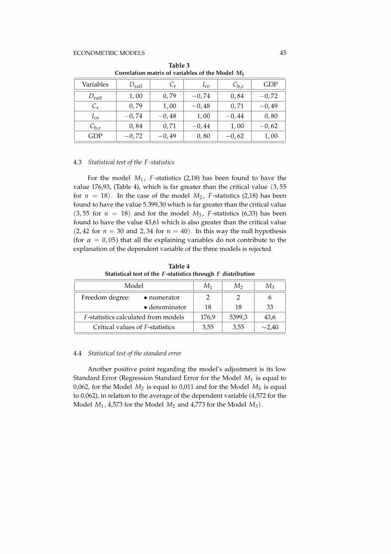
A prerequisite for the use of the independent variables in a modelis the absence of high correlation between the independent variables.Tables 1, 2 and 3 present the correlation matrix of the variables of theModels M1 , M2 and M3 . We can note the low correlation between theindependent variables and the high correlation of independent variableswith the dependent variable for each model.

Table 1Correlation matrix of variables of the Model M1

Variables Dtot GDP Cfuel

Dtot 1, 00 0, 68 −0, 93GDP 0, 68 1, 00 −0, 32Cfuel −0, 93 −0, 32 1, 00


Variables Dcar Ico Cfuel

Dcar 1, 00 0, 99 −0, 95Ico 0, 99 1, 00 −0, 52

Cfuel −0, 95 −0, 52 1, 00



Variables Drail Cr Ico Cb,r GDP

Drail 1, 00 0, 79 −0, 74 0, 84 −0, 72Cr 0, 79 1, 00 −0, 48 0, 71 −0, 49Ico −0, 74 −0, 48 1, 00 −0, 44 0, 80

Cb,r 0, 84 0, 71 −0, 44 1, 00 −0, 62GDP −0, 72 −0, 49 0, 80 −0, 62 1, 00

4.3 Statistical test of the F -statistics

For the model M1 , F -statistics (2,18) has been found to have thevalue 176,93, (Table 4), which is far greater than the critical value (3, 55for n = 18) . In the case of the model M2 , F -statistics (2,18) has beenfound to have the value 5.399,30 which is far greater than the critical value(3, 55 for n = 18) and for the model M3 , F -statistics (6,33) has beenfound to have the value 43,61 which is also greater than the critical value(2, 42 for n = 30 and 2, 34 for n = 40) . In this way the null hypothesis(for α = 0, 05) that all the explaining variables do not contribute to theexplanation of the dependent variable of the three models is rejected.

Table 4Statistical test of the F -statistics through F distribution

Model M1 M2 M3

Freedom degree: • numerator 2 2 6• denominator 18 18 33

F-statistics calculated from models 176,9 5399,3 43,6Critical values of F-statistics 3,55 3,55 ∼2,40

4.4 Statistical test of the standard error

Another positive point regarding the model’s adjustment is its lowStandard Error (Regression Standard Error for the Model M1 is equal to0,062, for the Model M2 is equal to 0,011 and for the Model M3 is equalto 0,062), in relation to the average of the dependent variable (4,572 for theModel M1 , 4,573 for the Model M2 and 4,773 for the Model M3) .


4.5 Model function form test

The diagnostic test, which examines the model’s function form, doesnot reject the null hypothesis that residuals are in accordance with thenormal distribution. The X2 distribution is equal to 0,083 for the ModelM1 , 0,690 for the Model M2 and 0,360 for the Model M3 , whereas thecritical value for one degree of freedom and a significance level of α =0, 05 is 3,841, (Table 5).

Table 5Econometric model’s residual diagnostic tests

Model→ Degree of freedom X2 Statistics CriticalM1 M2 M3 M1 M2 M3 values

Test ↓A: Serial correlation 1 1 1 2,326 2,462 0,774 3,841B: Functional form 1 1 1 0,083 0,690 0,360 3,841C: Normality 2 2 2 0,820 1,878 1,262 5,991D: Heteroscedasticity 1 1 1 1,366 2,271 0,301 3,841

A: Lagrange multiplier test of residual serial correlationB: Ramsey’s RESET test using the square of the fitted valuesC: Based on a test of skewness and kurtosis of residualsD: Based on the regression of squared residuals on squared fitted values

4.6 First degree self-correlation test to residuals

The absence of the three model residuals first degree self-correlationis also satisfactory. For the Model M1 , Durbin-Watson statistics was equalto 1,80, (which is very close to the optimum value of ±2, 00) and for theModel M2 was equal to 1,74. For the Model M3 and due to the fact that thedependent variable Drail has been included as an explaining variable witha time lag (Drail(−1)) , Durbin Watson statistics is not employed for theself-correlation test (Guthberston et al. 1992). In such cases, the Durbin’s-h statistics can be used, which has the value of −0, 58 , a result within thespace +1, 96÷−1, 96 .

4.7 Residuals correlation test

The lack of residual correlation for the three Models is confirmed bythe appropriate test, throughout the Lagrange multiplier test of residualsserial correlation, presented in Table 5. In the case of Model M3 , which


has a time lag dependent variable, the order of self-correlation check wasextended beyond one (order of self correlation = 2) , whereas the resultsdo not reject the null hypothesis in all cases.

4.8 Residuals normality

The diagnostic test that examines the pattern of distribution and itsparameters (residual normality) does not reject the null hypothesis thatresiduals are in accordance to the normal distribution. The X2 distributionis equal to 0,820 for the Model M1 , 1,878 for the Model M2 and 1,262 forthe Model M3 , whereas the critical value for two degrees of freedom anda significance level of α = 0, 05 is 5,991, (Table 5).

4.9 Residuals heteroscedasticity test

The residuals heteroscedasticity test showed that residuals have astandard fluctuation (homoscedastic error fluctuation) as the X2 distrib-ution’s value is 1,366 for the Model M1 , 2,271 for the Model M2 and 0,301for the Model M3 , whereas the critical value for one degree of freedomand a significance level of α = 0, 05 is 3,841, (Table 5).

4.10 Model stability test

In what regards the model’s stability and its robustness, the timeperiod of the sample used for the model’s adjustment is checked regardingits importance on the model’s form, through recursive regressions. Inorder to check the degree to which the model has been appropriatelyspecialized, the Cumulative Sum test (CUSUM), (Figures 7, 8 and 9) andthe Cumulative Sum Squared test (CUSUMQ), (Figures 10, 11 and 12) wereemployed. Figures 7 to 12 present the two tests with the critical levels for a5% significance level. If any of the two tests exceeds the critical values fora 5% significance level, then the null hypothesis that the model has beenappropriately specialized is rejected, (Maddala, 1992).

4.11 Model stability test through Chow’s statistical test (Predictive Failure Test)

In the case of the model M3, the presence of the dependent variablethrough a time lag, causes doubts about limits’ reliability, because anumber of cases have been reported in which the ability of the twotests to detect the parameters’ stability was considered unsatisfactory(Guthberston et al., 1992). Therefore, Chow’s second test must also beemployed, whereas the model’s robustness is tested through the Predictive


Figure 7Cumulative Sum test of recursive residuals (with critical limits) fora 5% significance level of the econometric model M1




Figure 10Cumulative Sum Squared test of recursive residuals (with criticallimits) for a 5% significance level of the econometric model M1




Failure Test. The test was used for the period 1961 ÷ 1998 for whichthe F(2, 32) statistics value was equal to 1,483. This value is less than thecorresponding critical value (3,23 for 40 periods that is years from 1960to 2000), which means that the null hypothesis for the model’s stabilitycannot be rejected.

5. Elasticities of the models

5.1 Total passenger demand elasticities

The validity of the model M1 is corroborated, besides the diagnostictests, with the signs of explaining variables and their elasticities, (Table 6):

• For the variable GDP (Gross Domestic Product of Greece) a positivesign was correctly calculated, since an income increase is expected tohave a positive influence on mobility.

• For the variable Cfuel (cost of fuel) a negative sign was correctlycalculated, since an in crease in the cost of fuel is expected to havea negative influence on mobility.

Table 6Elasticities of the independent variables of the Model M1

Independent variable Elasticity

Gross Domestic Product per capita (GDP) 1,667Cost of fuel (Cfuel) −0, 887

5.2 Private car demand elasticities

The elasticities of the econometric model M2 concerning the privatecar demand are given in Table 7. We can remark that:

Table 7Elasticities of the independent variables of the Model M2


Car ownership index (Ico) 0,691Cost of fuel (Cfuel) −0, 066

• For the variable Ico (car ownership index) a positive sign wascorrectly calculated since an increase in the car ownership index hasa positive influence on the use of car.


• For the variable Cfuel (cost of fuel) a negative sign was correctlycalculated, since an increase in the cost of use of private car isexpected to have a negative effect on its use.

• The importance of the constant c and its high value suggest that useof car is done regardless of other factors affecting private car demand.

5.3 Rail passenger demand elasticities

Elasticities of the econometric model M3 for rail passenger demandare given in Table 8. We can remark that:

• For the variable Cr (rail use cost per passenger-kilometer) a negativesign was correctly calculated, since an increase in a mode’s usecost has a negative effect on its transport demand. However, theappearance of the variable Cr three times as an independent vari-able (Cr, Cb,r, Dr(−1) suggests a short-run price elasticity of −0, 303(= 0, 192 − 0, 111) and a long-run elasticity of −1, 353 (−0, 303/

(1− 0, 776)) .

• For the variable Ico (car ownership index) a negative sign wascorrectly calculated, since an increase in the car ownership index hasan adverse effect on mass transport demand.

• For the variable Cb,r which expresses competition, a positive signwas correctly calculated because an increase on the ratio (bus usecost)/(rail use cost) has a positive impact on rail demand.

• For the variable GDP per capita, a positive sign was correctlycalculated, since an income increase is expected to have a positiveeffect on rail demand. The low value of the coefficient of the variable(0,111) suggests that rail transport is considered as a usual andnormal good (as opposed to luxury goods) and therefore its demandis not strongly affected by economic conditions.

• The variable which we should probably emphasize is Dr(−1) . Besidesits high importance in explaining demand ( t -student = +7, 54) , thisvariable has also the highest coefficient of all explaining variables(0,776). If services of Greek Railways (transport quality, employeebehavior, cleanliness, reliability) could be quantified, it could be saidthan a 1% increase in them would lead to 0,776% demand increase.


Table 8Elasticities of the independent variables of the model M3


Rail use cost per passenger-kilometer (Cr) −0, 192

Car ownership index (Ico) −0, 078

Competition variable, expressed as the cost 0,111

to use bus instead of railway per passenger-

kilometer (Cb,r)

Gross Domestic Product per capita (GDP) 0,109

Time lag dependent variable Drail(−1) 0,776

6. Forecasting ability of the proposed models

The forecasting ability of the proposed models is tested with theU-Theil Statistics method. This method allows the examination of resid-uals and appraisal of the forecasting ability by employing appropriatestatistical tests. When U-Theil Statistics is calculated equal to zero fora model, then the model’s forecasting ability is perfect, whereas whenU-Theil Statistics is calculated equal to one, the model lacks any forecast-ing ability (Jarret, 1987).

Through calculation of the U-Theil Statistics for the proposed econo-metric models, it is derived that the U-Theil Statistics has the value 0,125for the model M1 , the value 0,025 for the Model M2 and the value 0,244for the model M3 ; these values are very close to the ideal value, which, asexplained earlier, is zero.

7. Forecast of future modal split for Greece

Once the forecasting ability is checked, the models can be used forthe forecast of future demand and modal split for passenger transport forGreece, (Figures 13, 14).

8. Concluding remarks

It is essential in transport planning to establish a causal relationshipbetween the demand of each transport mode and the parameters affectingdemand. Such a causal analysis has been presented in this paper. Threeeconometric models have been proposed for passenger demand in Greece,


relating total demand, rail demand and private car demand to factorsaffecting each mode. The necessary appropriate tests assure the validityof the proposed models, which can then be used for the forecast of futuredemand.

Figure 13Forecast, with the use of econometric models (M1 , M2 , M3) , offuture demand of various transport modes in Greece

Figure 14Forecast, with the use of econometric models (M1 , M2 , M3) , ofmarket share of various transport modes in Greece

References

[1] C. Bhat and V. Pulugurta (1998), A comparison of two alternativesbehavioral choice mechanisms for household auto ownership deci-sion, Transportation Research B, Vol. 32 (1), pp. 61–75.

[2] P. Coppola and A. Carteni (2001), A study on the elasticity of long-range travel demand for passenger transport, Transporti Europei,Vol. 19, pp. 32–42.


[3] ECMT (European Conference of Ministers of Transport) (2001), As-sessing the Benefits of Transport, OECD Publications, Paris.

[4] EC (European Commission) (2004), EU energy and transport infigures – statistical pocketbook 2004, Office for Official Publications ofthe European Community, Belgium.

[5] T. Fowkes, C. Nash and A. Whiteing (1985), Understanding trendsin intercity rail travel in Great Britain, Transportation Planning &Technology, Vol. 10, p. 10.

[6] K. Guthberston, S. Hall and M. Taylor (1992), Applied EconometricTechniques, Harvester-Wheatleaf.

[7] J. Jarret (1987), Business Forecasting Methods, Blackwell.[8] P. M. Jones, M. C. Dix, M. I. Clarke and I. G. Heggie (1983),

Understanding Travel Behavior, Gower Publishing Co. Ltd., Aldeshort.[9] G. S. Maddala (1992), Introduction to Econometrics, MacMillan.

[10] R. Noland, J. Polak, M. Bell and N. Thorpe (2003), How muchdisruption to activities could fuel storages cause? The British FuelCrisis of September 2000, Transportation, Vol. 30, pp. 459–481.

[11] J. Ortuzar and L. Willumsen (1994), Modelling Transport, 2nd edn.,Wiley.

[12] F. Plassard (1996), Infrastructure-induced mobility, in ECMT RoundTable, Vol. 105, pp. 132–133, Paris.

[13] V. Profillidis (2004), Transport Economics, 3rd edn. (in Greek), Papa-sotiriou, Athens.

[14] A. Regianni and S. Stefani (1989), A new approach to modal splitanalysis, some empirical results, Transport Research B, Vol. 23 (1),pp. 75–82.

[15] P. Stopher and M. Lee-Gosselin (1996), Understanding Travel Behaviourin an Area of Change, Elsevier.

[16] Transport 2010 (1992), Commissariat General du Plan, DocumentationFrancaise, Paris.

[17] F. Wilson, S. Domodaran and J. Innes (1990), Disagregate modechoice models for intercity passenger travel in Canada, CanadianJournal of Civil Engineers, Vol. 17 (2), pp. 184–191.

Received May, 2005

econometric models for the forecast of - taru publications

Documents