econ 500 microeconomic theory consumer theoryebayrak/teaching/500f13/econ 500... · ·...
TRANSCRIPT
ECON 500
ECON 500 –Microeconomic Theory
Consumer Theory

ECON 500
Consumer Theory
A theory of how consumers allocate incomes among different goods and
services to maximize their well-being.
Part I Preferences and Utility
Part II Constraints and Choice
Part III Comparative Statics

ECON 500
Part I. Preferences and Utility
Axioms of Rational Choice
I. Completeness
II. Transitivity
III. Continuity

ECON 500
Part I. Preferences and Utility
Axioms of Rational Choice
I. Completeness
Consumers can compare and rank all possible baskets. Thus, for any
two market baskets A and B, a consumer will prefer A to B, will
prefer B to A, or will be indifferent between the two. By indifferent
we mean that a person will be equally satisfied with either basket.
Note that these preferences ignore costs. A consumer might prefer A
to B but buy only B because it is cheaper.

ECON 500
Part I. Preferences and Utility
Axioms of Rational Choice
I. Completeness
II. Transitivity
If a consumer prefers basket A to basket B and basket B to basket C, then
the consumer also prefers A to C. Transitivity ensures that the individual’s
choices are internally consistent.

ECON 500
Part I. Preferences and Utility
Axioms of Rational Choice
I. Completeness
II. Transitivity
III. Continuity
If A is preferred to B, then situations suitably “close to” A must also be
preferred to B. Enables the analysis of individuals’ responses to relatively
small changes in income and prices
ECON 500
Part I. Preferences and Utility
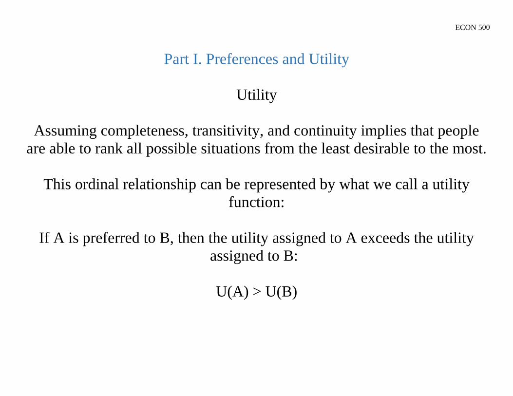
Utility
Assuming completeness, transitivity, and continuity implies that people
are able to rank all possible situations from the least desirable to the most.
This ordinal relationship can be represented by what we call a utility
function:
If A is preferred to B, then the utility assigned to A exceeds the utility
assigned to B:
U(A) > U(B)

ECON 500
Part I. Preferences and Utility
Utility
Individuals’ preferences are assumed to be represented by a utility
function of the form U(x1, x2, . . . , xn , Z )
Where x1, x2,…, xn are the quantities of each of n goods that might be
consumed in a period, and Z is everything else.
Ceteris Paribus assumption allows us to drop Z.
This function is unique only up to an order-preserving (monotone)
transformation

ECON 500
Part I. Preferences and Utility
Utility
The ordinal nature of utility and the non-uniqueness of utility functions
makes them:
Useful in analyzing only the relative desirability of choices
No so useful in analyzing absolute utility gains across bundles
Not so useful in making interpersonal comparisons

ECON 500
Part I. Preferences and Utility
Utility
Arguments of utility functions
U(W) = utility an individual receives from real wealth (W)
U(c,h) = utility from consumption (c) and leisure (h)
U(c1,c2) = utility from consumption in two different periods
Two-good utility function U(x,y)
More of any particular xi during some period is preferred to less

ECON 500
Part I. Preferences and Utility
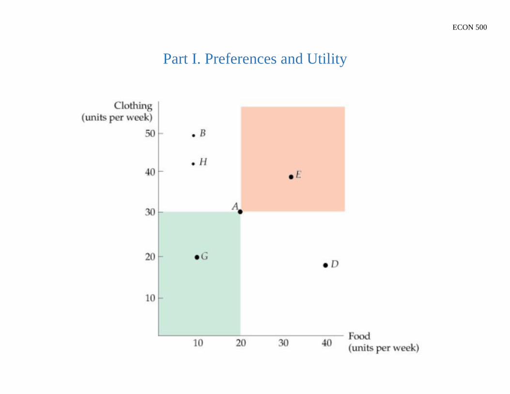
Alternative Market Bundles
Bundle Units of Food Units of Clothing
A 20 30
B 10 50
D 40 20
E 30 40
G 10 20
H 10 40

ECON 500
Part I. Preferences and Utility

ECON 500
Part I. Preferences and Utility
Indifference Curve:
Shows a set of consumption bundles that provide the consumer
with the same level of utility.
The consumer ranks these bundles equally, in other words the consumer is
indifferent about consuming any bundle on the indifference curve
ECON 500
Part I. Preferences and Utility

ECON 500
Part I. Preferences and Utility
ECON 500
Part I. Preferences and Utility
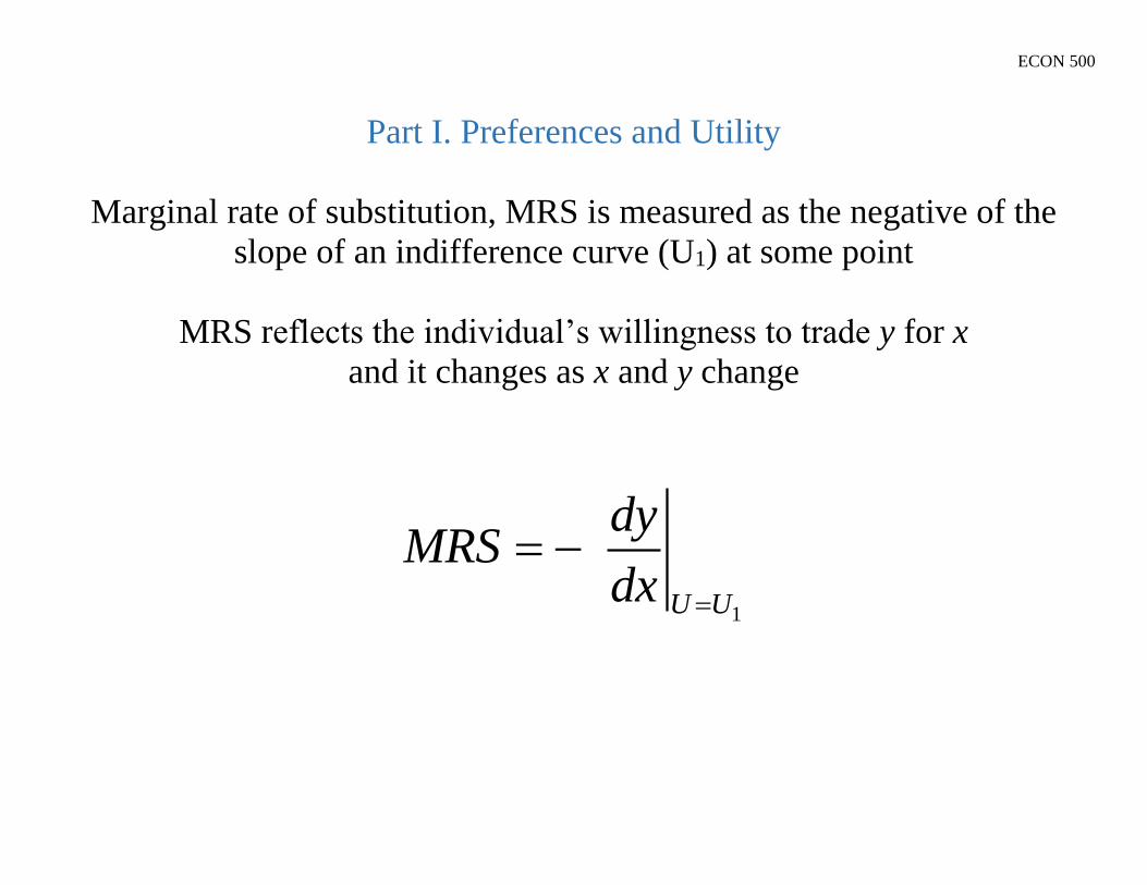
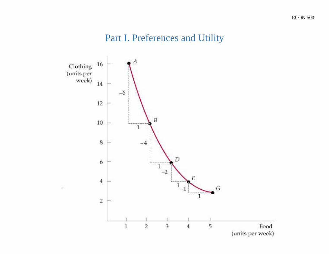
Marginal rate of substitution, MRS is measured as the negative of the
slope of an indifference curve (U1) at some point
MRS reflects the individual’s willingness to trade y for x
and it changes as x and y change
1
U U
dyMRS
dx
ECON 500
Part I. Preferences and Utility

ECON 500
Part I. Preferences and Utility
MRS=?
ECON 500
Part I. Preferences and Utility
Indifference Curves and Transitivity
ECON 500
Part I. Preferences and Utility
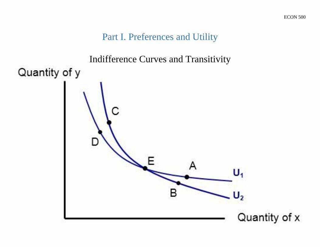
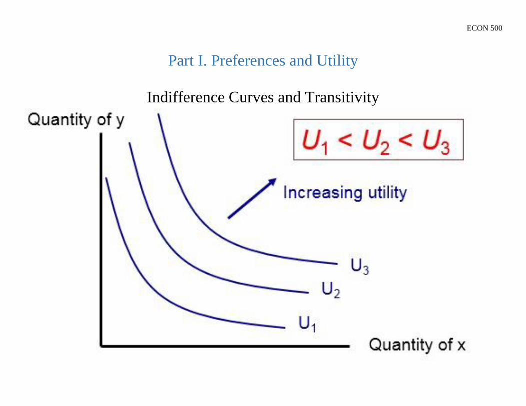
Indifference Curves and Transitivity
The transitivity axiom implies that indifference curves cannot intersect.
There is a single indifference curve that passes through every point in the
goods space, in other words every bundle is associated with a unique
utility level.
ECON 500
Part I. Preferences and Utility
Indifference Curves and Transitivity
ECON 500
Part I. Preferences and Utility
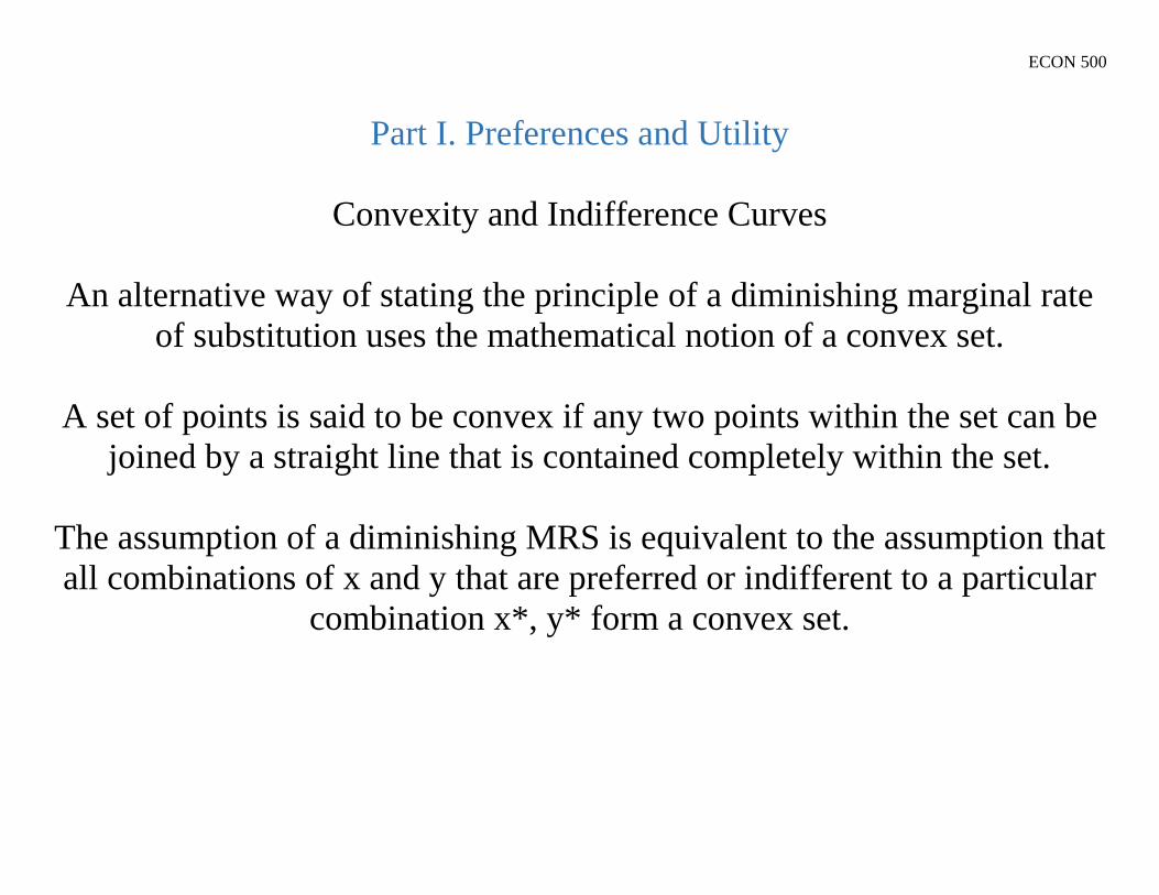
Convexity and Indifference Curves
An alternative way of stating the principle of a diminishing marginal rate
of substitution uses the mathematical notion of a convex set.
A set of points is said to be convex if any two points within the set can be
joined by a straight line that is contained completely within the set.
The assumption of a diminishing MRS is equivalent to the assumption that
all combinations of x and y that are preferred or indifferent to a particular
combination x*, y* form a convex set.
ECON 500
Part I. Preferences and Utility
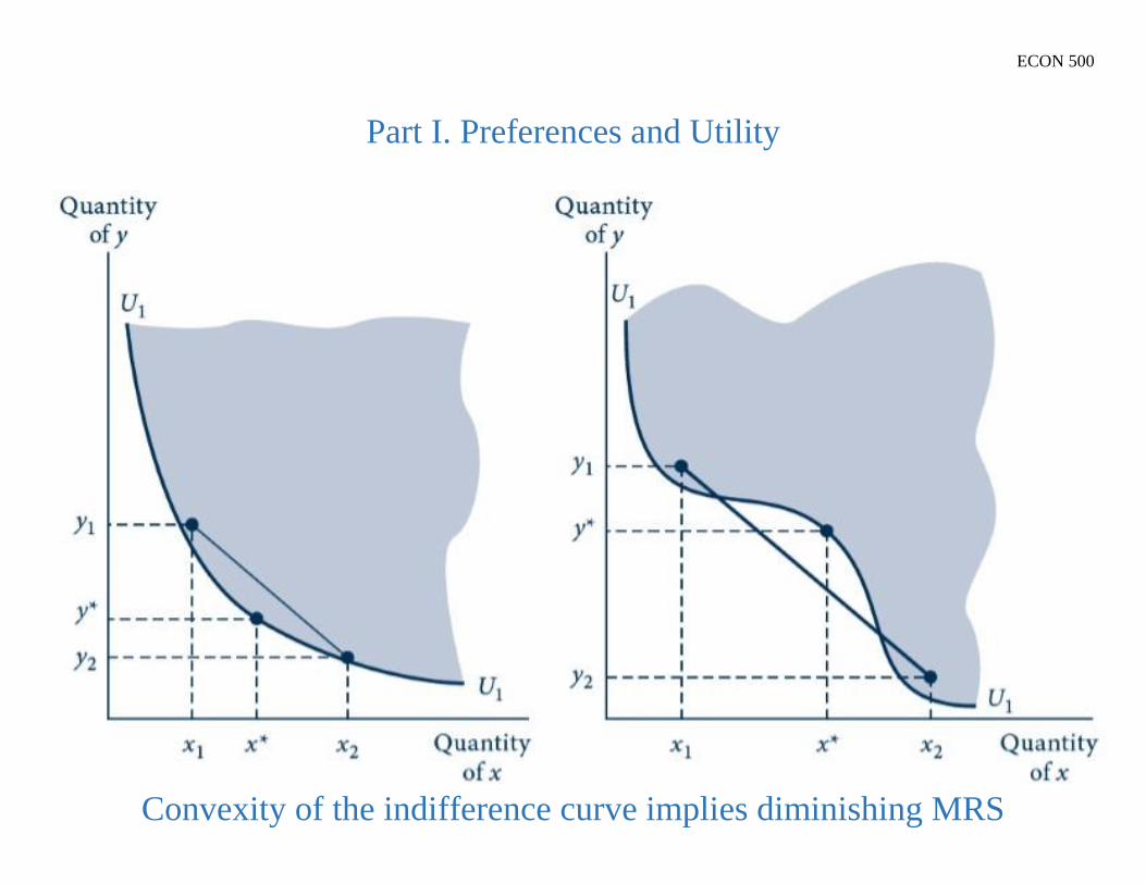
Convexity of the indifference curve implies diminishing MRS

ECON 500
Part I. Preferences and Utility
Convexity and Balance in Consumption
If indifference curves are convex (if they obey the assumption of a
diminishing MRS), then the line joining any two points that are indifferent
will contain points preferred to either of the initial combinations.
Intuitively, balanced bundles are preferred to unbalanced ones.

ECON 500
Part I. Preferences and Utility

ECON 500
Part I. Preferences and Utility
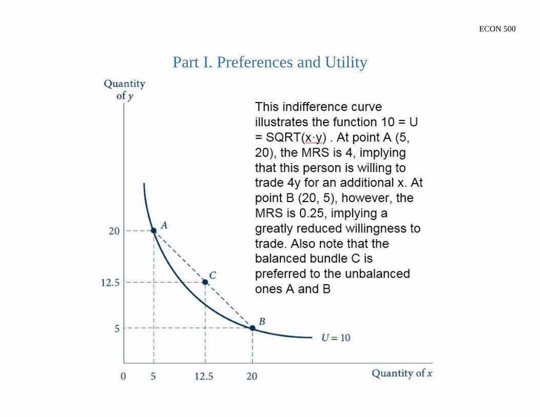
Suppose the utility function s of the form
U =
An indifference curve for this function that set of combinations of x
and y for which utility has the value 10 is:
10 =
Rearranging:
100=x·y
y=100/x
MRS = -dy/dx(along U1)=100/x2
As x rises, MRS falls
When x = 5, MRS = 4
When x = 20, MRS = 0.25
ECON 500
Part I. Preferences and Utility
ECON 500
Part I. Preferences and Utility
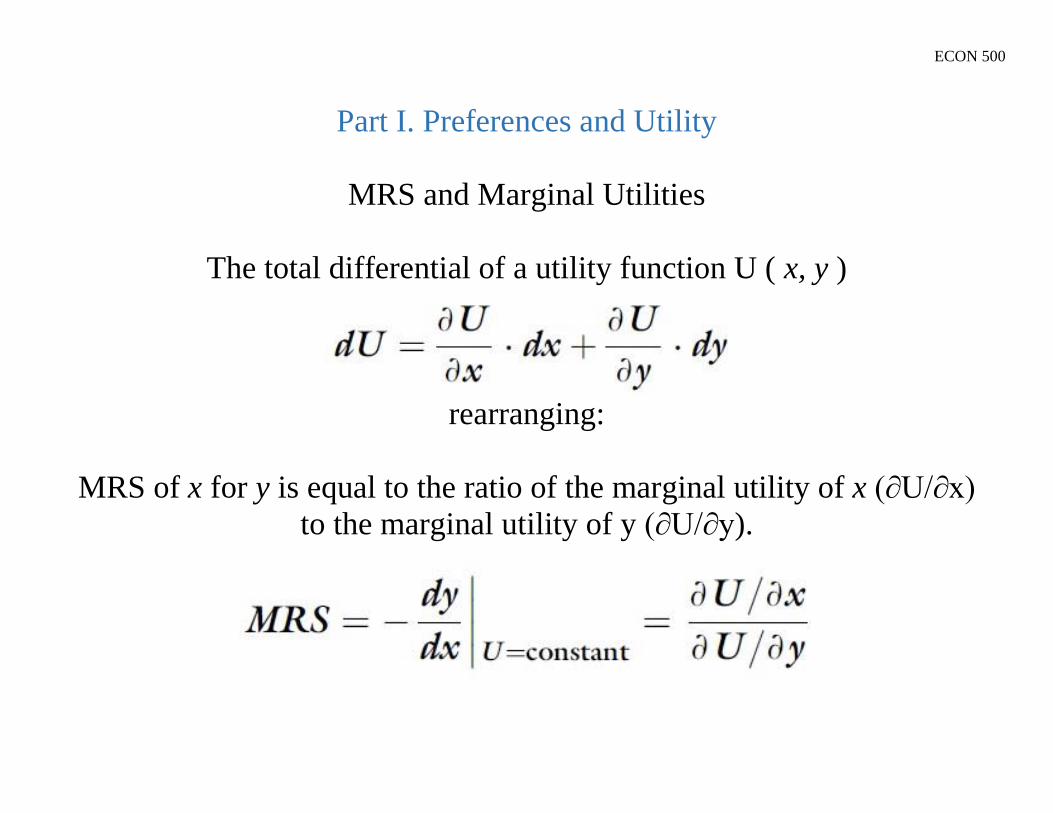
MRS and Marginal Utilities
The total differential of a utility function U ( x, y )
rearranging:
MRS of x for y is equal to the ratio of the marginal utility of x (∂U/∂x)
to the marginal utility of y (∂U/∂y).

ECON 500
Part I. Preferences and Utility
Cobb-Douglas Utility
U(x,y) = xy
Where and are positive constants
The relative sizes of and indicate the relative importance of the goods
We can normalize + = 1 by an invariant monotonic transformation
U(x,y) = xy1-
Where =/(+) and 1-=/(+)

ECON 500
Part I. Preferences and Utility
Perfect substitutes
U(x,y) = x + y
Where and are positive constants
The MRS will be constant along the linear indifference curves
Perfect complements
U(x,y) = min (x, y)
Where and are positive parameters
L-shaped indifference curves
ECON 500
Part I. Preferences and Utility
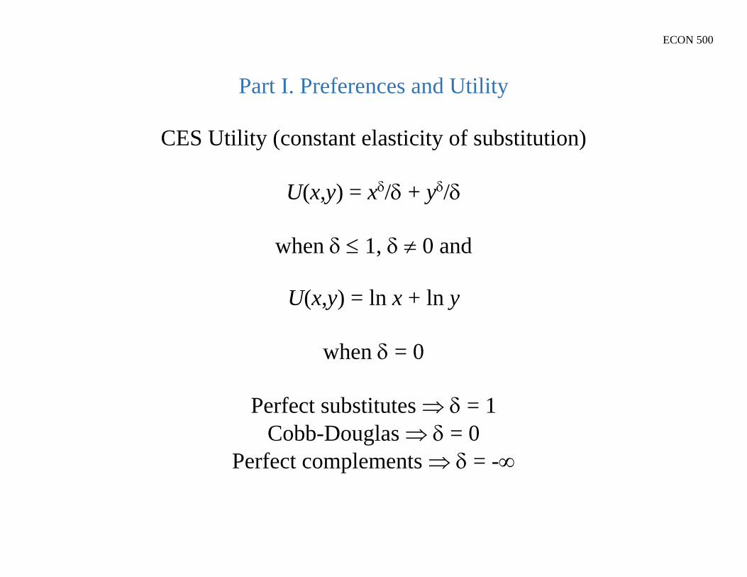
CES Utility (constant elasticity of substitution)
U(x,y) = x/ + y/
when 1, 0 and
U(x,y) = ln x + ln y
when = 0
Perfect substitutes = 1
Cobb-Douglas = 0
Perfect complements = -
ECON 500
Part I. Preferences and Utility
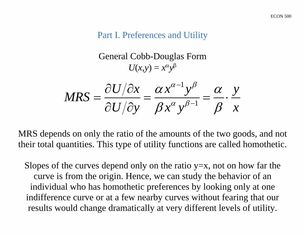
General Cobb-Douglas Form
U(x,y) = xy
MRS depends on only the ratio of the amounts of the two goods, and not
their total quantities. This type of utility functions are called homothetic.
Slopes of the curves depend only on the ratio y=x, not on how far the
curve is from the origin. Hence, we can study the behavior of an
individual who has homothetic preferences by looking only at one
indifference curve or at a few nearby curves without fearing that our
results would change dramatically at very different levels of utility.
1
1
U x x y yMRS
U y x y x
ECON 500
Part I. Preferences and Utility
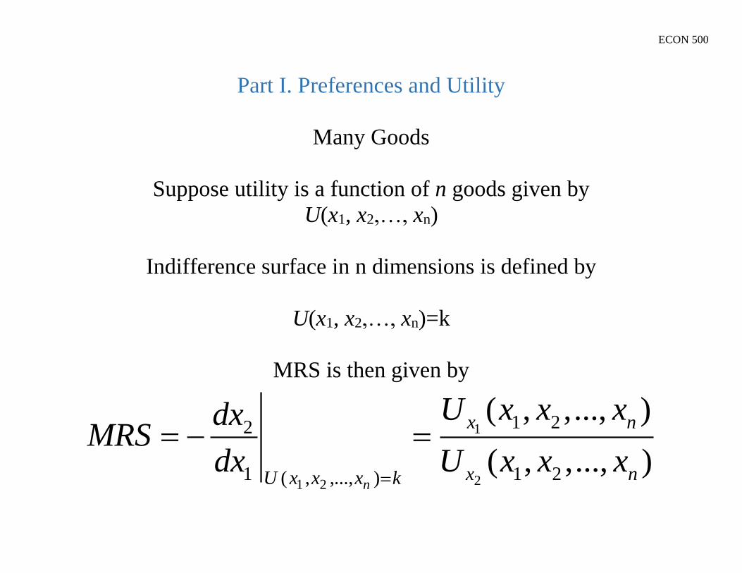
Many Goods
Suppose utility is a function of n goods given by
U(x1, x2,…, xn)
Indifference surface in n dimensions is defined by
U(x1, x2,…, xn)=k
MRS is then given by
1
21 2
1 22
1 1 2( , ,..., )
( , ,..., )
( , ,..., )n
x n
x nU x x x k
U x x xdxMRS
dx U x x x
ECON 500
Part II. Constraints and Choice
Basic Model of Consumer Choice: Utility Maximization
This model assumes that individuals who are constrained by limited
incomes will behave as if they are using their purchasing power in such a
way as to achieve the highest utility possible.
That is, individuals are assumed to behave as if they maximize utility
subject to a budget constraint.

ECON 500
Part II. Constraints and Choice
Basic Model of Consumer Choice: Utility Maximization
Two Concerns:
Do individuals make the “lightning calculations” required for utility
maximization?
Is the economic model of choice is extremely selfish?
ECON 500
Part II. Constraints and Choice
To maximize utility, his or her preferences and a fixed amount of income
to spend an individual will buy those quantities of goods:
a) That exhaust his or her total income
b) and for which the MRS is equal to the rate at which
the goods can be traded one for the other in the marketplace
MRS (of x for y) = the ratio of the price of x to the price of y (px/py)
ECON 500
Part II. Constraints and Choice
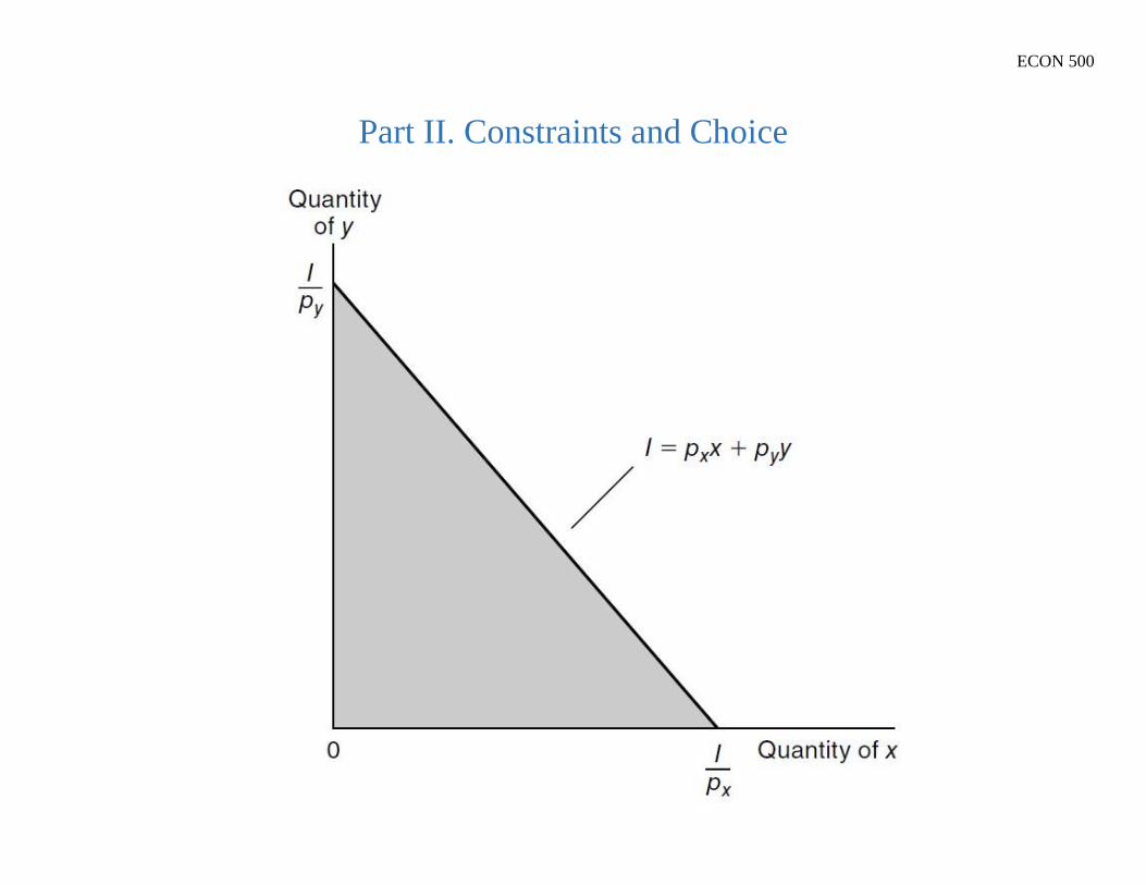
Additional Assumptions
I = Budget to allocate between good x and good y
px = price of good x
py = price of good y
Budget constraint:
pxx + pyy ≤ I
Slope = -px/py
If all of I is spent on good x(y), I/px(y) units of good x(y) can be bought
ECON 500
Part II. Constraints and Choice

ECON 500
Part II. Constraints and Choice

ECON 500
Part II. Constraints and Choice
Conditions (Necessary) for a maximum
Point of tangency between the budget constraint
and the indifference curve:
ECON 500
Part II. Constraints and Choice
The tangency rule is necessary but not sufficient
Unless we assume that MRS is diminishing
If MRS is diminishing, then indifference curves are strictly convex and
first order conditions are necessary AND sufficient
If MRS is not diminishing, one must check second-order conditions to
ensure that we are at a maximum

ECON 500
Part II. Constraints and Choice
ECON 500
Part II. Constraints and Choice
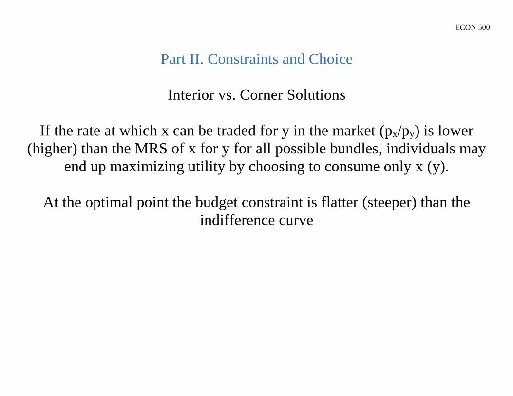
Interior vs. Corner Solutions
If the rate at which x can be traded for y in the market (px/py) is lower
(higher) than the MRS of x for y for all possible bundles, individuals may
end up maximizing utility by choosing to consume only x (y).
At the optimal point the budget constraint is flatter (steeper) than the
indifference curve

ECON 500
Part II. Constraints and Choice

ECON 500
Part II. Constraints and Choice
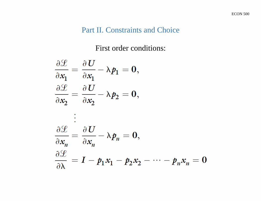
In the case of n-goods, consumer maximizes the utility
subject to:
To find the maximum s.t. the constraint we set up the Lagrangian:
Taking the partial derivatives of Lagrangian w.r.t x1,x2,…,xn, and λ, and
setting them equal to zero yields the n+1 necessary conditions for an
interior maximum.
ECON 500
Part II. Constraints and Choice
First order conditions:

ECON 500
Part II. Constraints and Choice
Rearranging the first order conditions yields that
for any two goods xi and xj
where the left hand side is the ratio of the marginal utilities, which have
derived to be the Marginal Rate of Substitution between xi and xj
ECON 500
Part II. Constraints and Choice
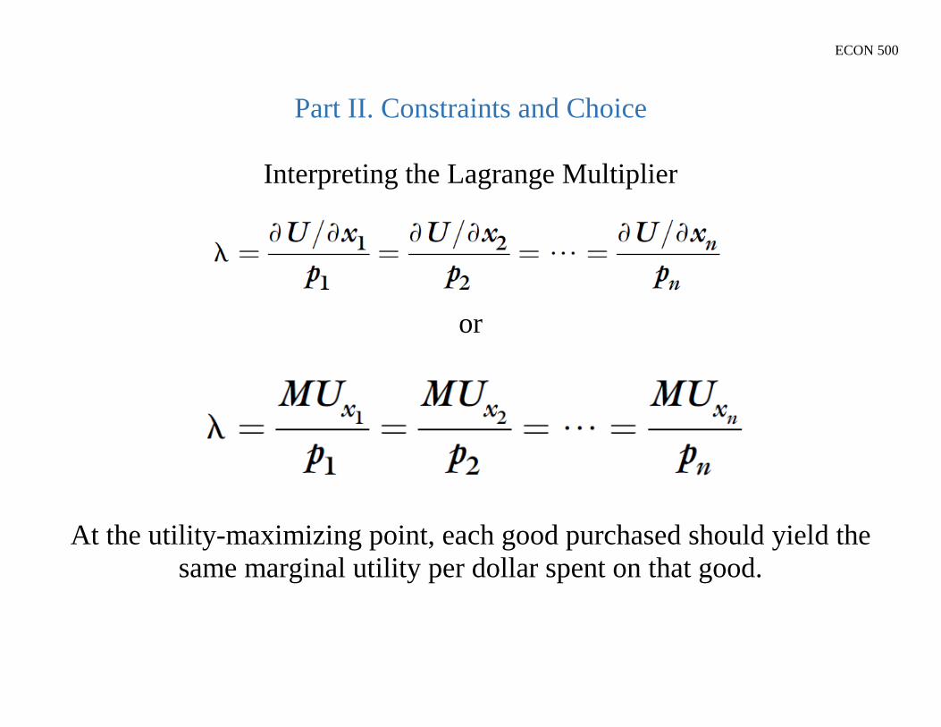
Interpreting the Lagrange Multiplier
or
At the utility-maximizing point, each good purchased should yield the
same marginal utility per dollar spent on that good.

ECON 500
Part II. Constraints and Choice
Cobb-Douglas Example (α + β = 1)
Lagrangian
FOCs
ECON 500
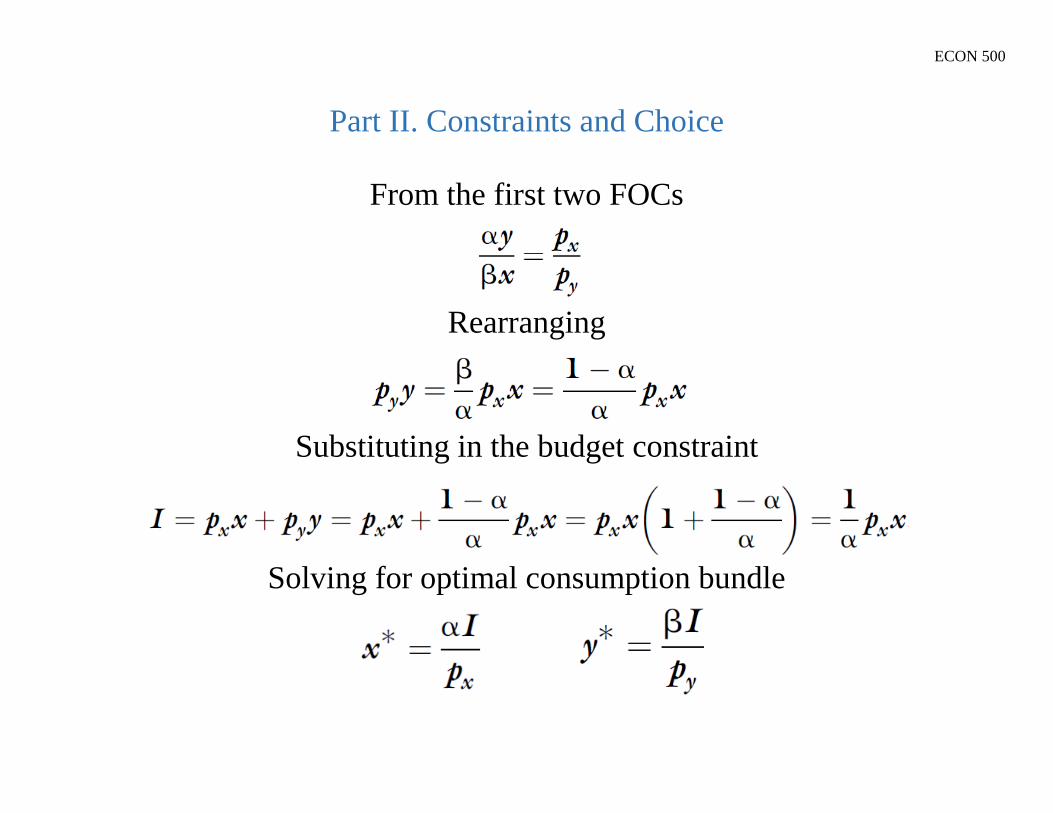
Part II. Constraints and Choice
From the first two FOCs
Rearranging
Substituting in the budget constraint
Solving for optimal consumption bundle

ECON 500
Part II. Constraints and Choice
Indirect Utility Function
We can solve for the optimum consumption bundles from the FOCs as a
function of prices and income
We can substitute the optimum bundles back into the utility function to
find maximum utility attainable given prices and income
ECON 500
Part II. Constraints and Choice
Lump Sum Principle
Lump sum income taxes or subsidies are superior to good-specific taxes or
subsidies in terms of their impact on consumer well-being.
The intuition is that the lump sum transfers leave the individual free to
decide how to allocate the final income across various good.
Good-specific taxes or subsidies not only impact purchasing power but
also distort choices by artificially distorting prices.

ECON 500
Part II. Constraints and Choice

ECON 500
Part II. Constraints and Choice
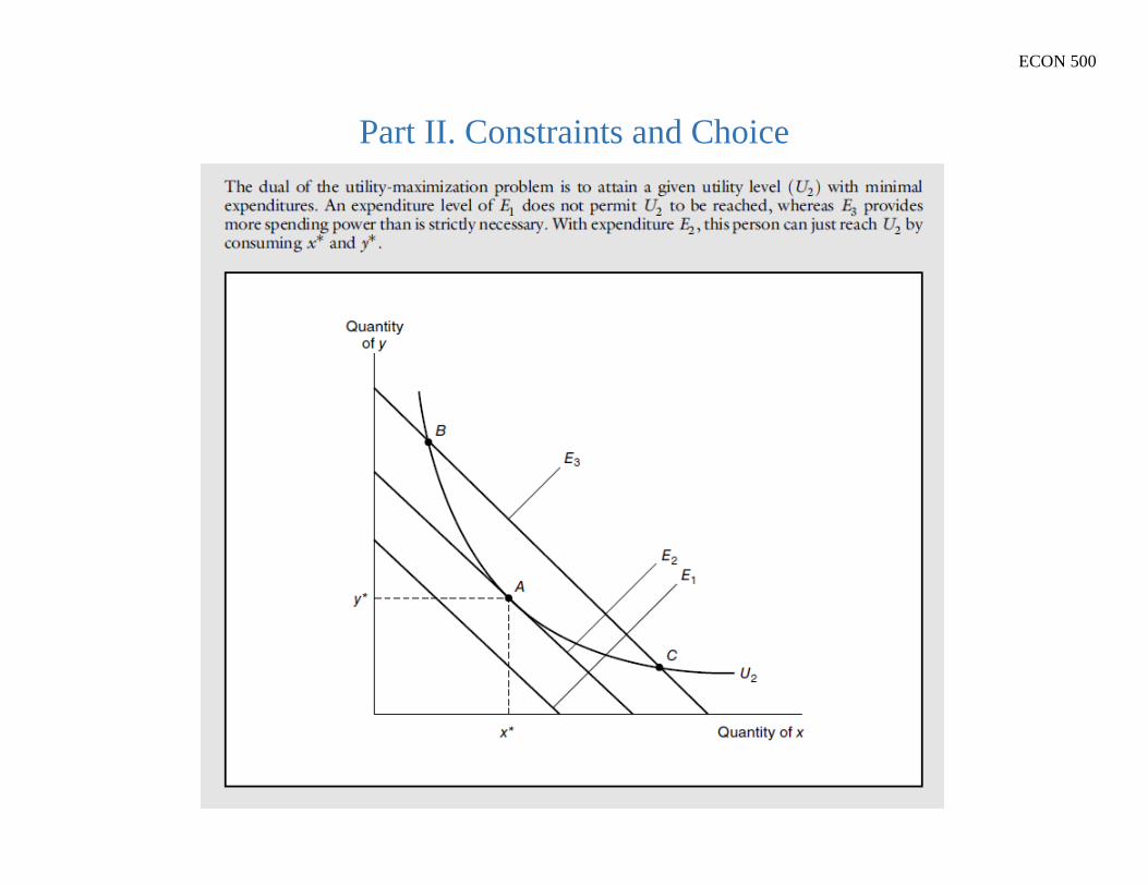
Duality
Utility maximization subject to a budget constraint is equivalent to
expenditure minimization subject to a utility target. This duality allows us
to employ the expenditure minimization approach in certain cases where
it is more useful due to the direct observability of expenditures.
The dual problem is to choose x1, …, xn to minimize
subject to
ECON 500
Part II. Constraints and Choice
ECON 500
Part III. Comparative Statics
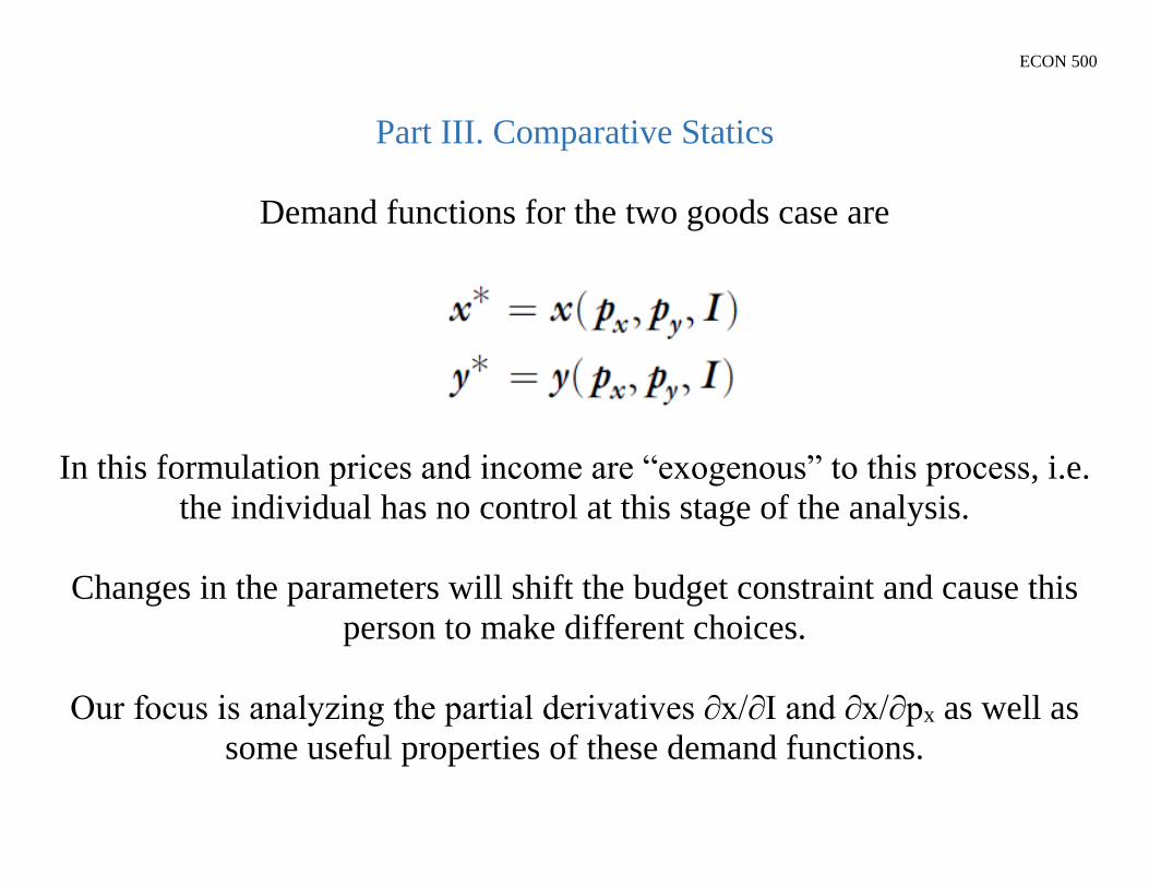
Demand functions for the two goods case are
In this formulation prices and income are “exogenous” to this process, i.e.
the individual has no control at this stage of the analysis.
Changes in the parameters will shift the budget constraint and cause this
person to make different choices.
Our focus is analyzing the partial derivatives ∂x/∂I and ∂x/∂px as well as
some useful properties of these demand functions.

ECON 500
Part III. Comparative Statics
Homogeneity
Functions that obey this property are said to be
homogeneous of degree zero.
If we were to double all prices and income simultaneously (or multiply
them all by any positive constant), then the optimal quantities demanded
would remain unchanged.
Changing all prices and income changes only the units by which we count,
not the “real” quantity of goods demanded.

ECON 500
Part III. Comparative Statics
Changes in Income
As a person’s purchasing power rises, it is natural to expect that the
quantity of each good purchased will also increase.
Changes in income shift the budget lines in a parallel fashion, reflecting
that the relative prices of x and y remain unchanged. Because the ratio
px/py stays constant, the utility-maximizing conditions also require that the
MRS stay constant as the individual moves to higher levels of satisfaction.
However, the point of tangency might or might not be on an upward
sloping expansion path with increasing consumption levels.
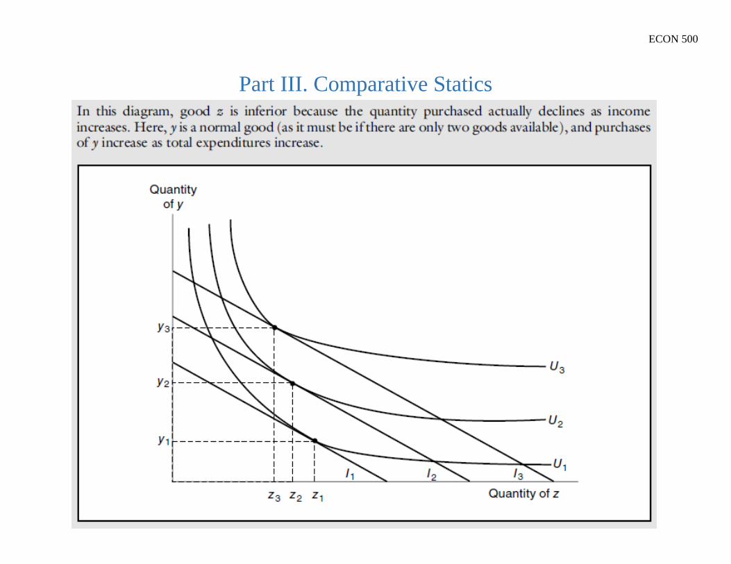
If ∂xi/∂I=0 over some range of income variation then the good is a normal
(or “noninferior”) good in that range. A good xi for which ∂xi/∂I < 0 over
some range of income changes is an inferior good in that range.

ECON 500
Part III. Comparative Statics
ECON 500
Part III. Comparative Statics

ECON 500
Part III. Comparative Statics
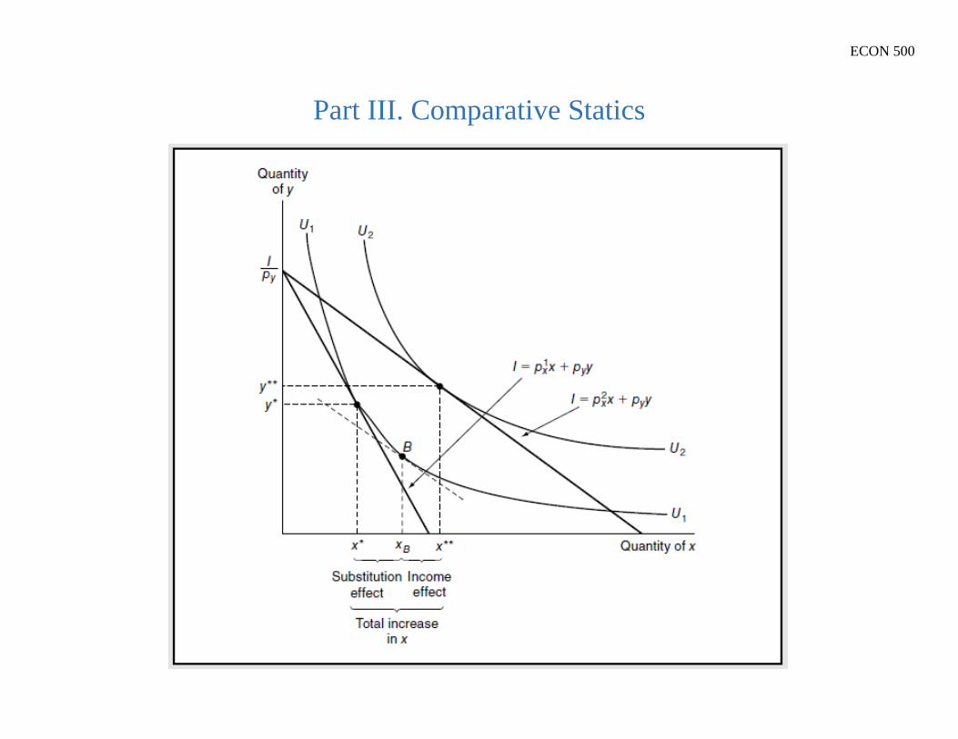
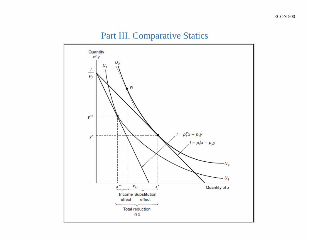
Changes in Prices
Changing a price involves changing not only the intercepts of the budget
constraint but also its slope. Therefore, when a price changes, two
analytically different effects come into play.
One of these is a substitution effect: even if the individual were to stay on
the same indifference curve, consumption patterns would be changed so as
to equate the MRS to the new price ratio.
A second effect, the income effect, arises because a price change
necessarily changes an individual’s “real” income. The individual cannot
stay on the initial indifference curve and must move to a new one.
ECON 500
Part III. Comparative Statics
ECON 500
Part III. Comparative Statics

ECON 500
Part III. Comparative Statics
In the case of inferior goods, income and substitution effects work in
opposite directions, and the combined result of a price change is
indeterminate.
A fall in price, will always cause an individual to tend to consume more of
a good because of the substitution effect. But if the good is inferior, the
increase in purchasing power caused by the price decline may cause less
of the good to be bought.
Unlike the situation for normal goods, it is not possible here to
predict even the direction of the effect of a change in px on the quantity of
x consumed and if the income effect of a price change is strong enough,
the change in price and the resulting change in the quantity demanded
could actually move in the same direction, which is called Giffen’s
Paradox
ECON 500
Part III. Comparative Statics
Individual’s (Uncompensated) Demand Curve
The demand curve looks at the relationship between x and px while
holding py, I, preferences and all other determinants constant.

ECON 500

ECON 500
Part III. Comparative Statics
Compensated Demand Curve
A compensated demand curve shows the relationship between the price of
a good and the quantity purchased on the assumption that other prices and
utility are held constant.
It therefore illustrates only substitution effects and isolates the analysis
from income effects. The choice between compensated and
uncompensated demand curves depends on the application at hand.
Mathematically, the curve is a two-dimensional representation of the
compensated demand function:

ECON 500

ECON 500
Part III. Comparative Statics
Suppose the utility function is of the form
Then the Marshallian demand functions are
The indirect utility function is then
Rearranging and substituting into the demand function reveals

ECON 500
Part III. Comparative Statics
Relationship between Compensated and Uncompensated Demand

ECON 500