ECON 4335 The economics of banking

Lecture 8, 20/3-2013: Credit rationing, importance ofinitial wealth, and pecuniary externalities

Bent Vale,Norges Bank∗

∗Views and conclusions are those of the lecturer and can not beattributed to Norges Bank

• Credit rationing:

— Among seemingly identical borrowers who are willing to pay the pre-vailing loan rate in the market some are denied any credit.There is an excess demand for credit.†

— Among identifiable different groups of borrowers some groups are de-nied credit at any loan rate. I.e., they are considered not creditworthy.

• How can such rationing appear in an unregulated market? Why cannotthe price of credit, the interest rate, clear the market?

†Another type of credit rationing: All borrowers get some credit, but not as much as theydemand at the prevailing loan rate in the market. Also excess demand, but we do not lookat this type of rationing in this lecture.

Theories explaining credit rationing

• Adverse selection (Stiglitz and Weiss (1981))

— But Arnold and Riley (2009) showed that adverse selection can hardlygenerate credit rationing as in SW.

• Moral hazard, i.e., unobservable actions (also in Stiglitz and Weiss (1981))

— risk shifting (SW), unobservable effort (this lecture)

• Unobservable state, or bankruptcy cost.

• These theories implies: initial distribution of wealth matters for effi ciency.

— At odds with standard new classical welfare theory: a first best, i.e.,PO, equilibrium can arise from any initial distribution of goods. Thiswelfare theorem is only valid under complete and perfect markets.

• When distribution of wealth matters for effi ciency⇒ pecuniary externalitieswill have effects on the effi ciency of the real economy.

• This can explain how changes in asset prices can have macroeconomicimpacts.

Model

• The demand side, behavior of non-financial firms as borrowers.

• Banks and the supply schedule in the credit market.

• Derive a demand schedule.

• Characterize the market

• How firms’equity position influences the credit market.

• Credit rationing, creditworthiness

Some implications for effects of pecuniary externalities

Borrowers

• N identical (except for one characteristic) risk neutral firms each have aninitial wealth a < 1. Each of them has access to a project where theyin period 1 can invest 1. The project will yield y > 1 in period 2 withprobability p, and 0 with probability (1− p).

• Success probability depends on the borrowers unobservable effort e, s.t.

0 ≤ p = p(e) ≤ 1, p′(e) > 0, p′′(e) < 0 .

• Since a < 1 a firm needs to borrow at interest rate r to be able to invest.Assume the borrowing firm’s cost of effort is e.

• Borrowing firms have limited liability.

• In addition, in order to carry out the investment each borrower needs todo some installation effort β right before e in period 1.

• β varies continuously among borrowers. So far, the only difference betweenborrowers. Introduced in order to get a downward sloping demand curve.

• Distribution β described by a density function g(β), where β ∈ [β, β].Hence: ∫ β

βg(β)dβ ≡ G(β) = N .

• Period 2 profit of the borrowing firm is

Eπ = p(e)[y − (1− a)(1 + r)]− a(1 + i)− (1 + i)(e+ β) ≡ V (e)

where i is the risk-free interest rate. For the given β, the firm decides itsoptimal effort according to 1. order condition

∂Eπ

∂e= [y − (1− a)(1 + r)]p′(e)− (1 + i) = 0

with 2nd. order condition

∂2Eπ

∂e2= [y − (1− a)(1 + r)]p′′(e) < 0

Note that the firm’s optimal e is independent of β.

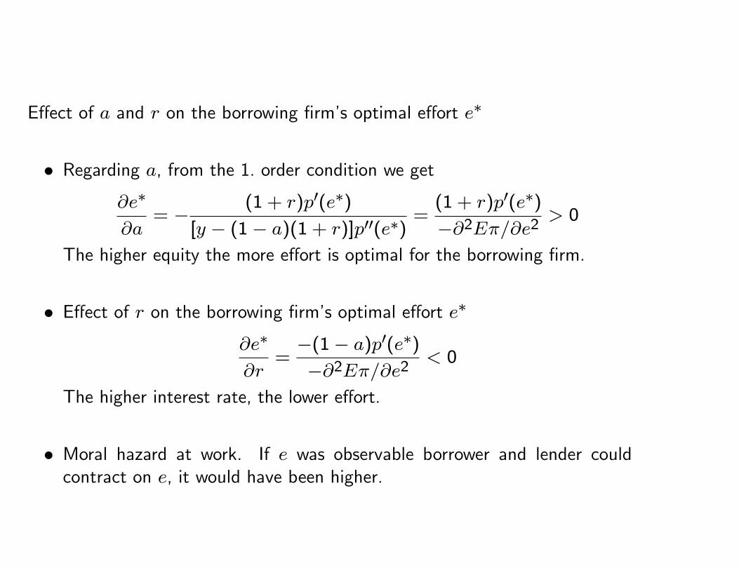
Effect of a and r on the borrowing firm’s optimal effort e∗

• Regarding a, from the 1. order condition we get

∂e∗

∂a= − (1 + r)p′(e∗)

[y − (1− a)(1 + r)]p′′(e∗)=(1 + r)p′(e∗)−∂2Eπ/∂e2

> 0

The higher equity the more effort is optimal for the borrowing firm.

• Effect of r on the borrowing firm’s optimal effort e∗

∂e∗

∂r=−(1− a)p′(e∗)−∂2Eπ/∂e2

< 0

The higher interest rate, the lower effort.

• Moral hazard at work. If e was observable borrower and lender couldcontract on e, it would have been higher.

Banks and the supply side in the credit marked.

• Several risk neutral banks compete a la Bertrand in offering loans to thefirms. Banks fund themselves at the risk-free interest rate (no equity inthe banks). I.e. in this market banks lend at zero expected profits.

p(e∗)(1− a)(1 + r)− (1− a)(1 + i) = 0i.e.

1 + r = 1+ip(e∗) or p(e∗)(1 + r) = 1 + i

Note that r is independent of how much the bank lends, a horizontal supplyschedule.I.e., we cannot have credit rationing as defined in the first bullet point onthe first slide in this model.

• However, can have an equilibrium where an identifiable group of borrowersdo not receive loans, i.e., not considered creditworthy.

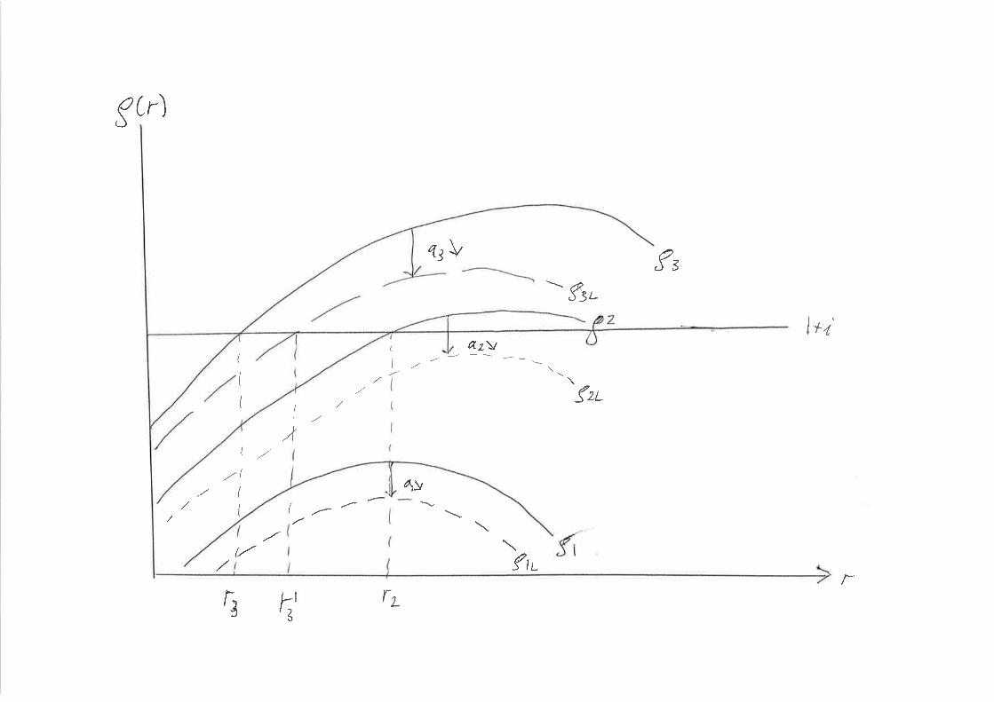
• Denote banks’gross return on lending p(e∗)(1 + r) by ρ(r) . Then wehave

ρ′(r) = p(e∗) + (1 + r)p′(e∗)∂e

∂r≶ 0

Thus, we can have concave relation between ρ and r. Since banks cannotobserve borrowers’effort e, in setting r banks have to take into accountthe negative effect of higher r on e. Let ρmax be the maximum value ofρ.

• If, nevertheless, 1 + i > ρmax then lending will be unprofitable. Theseborrowers not creditworthy. Will return to this case.

Demand side in the credit market.

• Firms have different βs, and only firms with E(π) ≥ 0 will demand a loan.Define β∗ s.t. E(π | β∗) = 0.

β∗ =[y − (1− a)(1 + r)]p(e∗)

1 + i− a− e∗

I.e., only borrowers with β < β∗ will demand a loan.

• With a horizontal supply schedule, all borrowers demanding credit willobtain it and carry out investments as long as 1 + i ≤ ρmax. Let K bethe number of investment projects that are carried out.

K = G(β∗) ≤ N , dK

dβ∗= g(β∗) > 0

• Inserting the expression for β∗ into the expression for K we get the fol-lowing properties of the demand schedule:

∂K∂r = −p(e

∗)(1−a)1+i g(β∗) < 0

∂K∂i = −[y−(1−a)(1+r)]p(e

∗)(1+i)2

g(β∗) < 0

∂K∂a =

(p(e∗)(1+r)

1+i − 1)g(β∗) = 0 follows from banks’0-profit condition

The credit market equilibrium.

• a, i and y are exogenous. Equilibrium e∗ and r are determined by borrow-ers’1. order condition and banks’zero profit condition. K follows fromG(β∗) and the expression for β∗ with the equilibrium e∗ and r inserted.

How lower borrower equity affects market equilibrium.

• The demand schedule is unaffected

• The supply schedule

— Know that for a given r lower equity will reduce e∗ thus p(e) down.Banks raise r to maintain zero-profit condition.

— Higher r implies further reduction in e∗, and higher r, and so on. Totaldifferentiation of banks’zero-profit condition

dr

da=

−(1 + r)p′(e∗)∂e∂ap(e∗) + (1 + r)p′(e∗)∂e∂r

< 0

I.e., lower a shifts the supply schedule upwards.

• Lower a implies higher r and fewer firms that demand loan and carries outinvestment projects, K ↘.

If effort could be observed perfectly

• The borrowing firm could commit to a certain effort. The contract betweena bank and a borrowing firm would specify both r and e.

— The equilibrium contract would be the one that maximized firms’ex-pected profits E(π) s.t. banks’zero expected profit condition. That isthe following Lagrange problem

maxe,r

H(e, r) = p(e)[y − (1− a)(1 + r)]− a(1 + i)− (1 + i)(e+ β)

−λ[(1 + i)(1− a)− (1− a)(1 + r)p(e)]

Solution:

yp′(e) = 1 + i(1 + r)p(e) = 1 + i

• Note, if effort was observable and contractable equilibrium e and r andthus K would be independent of a.

• In a first best equilibrium initial distribution of goods does not matter forthe effi ciency of the equilibrium.

Back to unobservable effort.

• ρ(r; a) = p (e∗) (1 + r). For any given r we have

∂ρ

∂a= (1 + r)p′(e∗)

∂e

∂a< 0

• Let a vary between groups of borrowers s.t. a1 < a2 Then ρ(r; a1) <ρ(r; a2) for any r.

• Define r∗1as the solution to maxr ρ(r; a1). Then we may haveρ(r∗1; a1) < 1 + i < ρ(r∗2; a2).

• Thus group 1 is rationed, all denied credit, but all borrowers in group 2obtain credit.

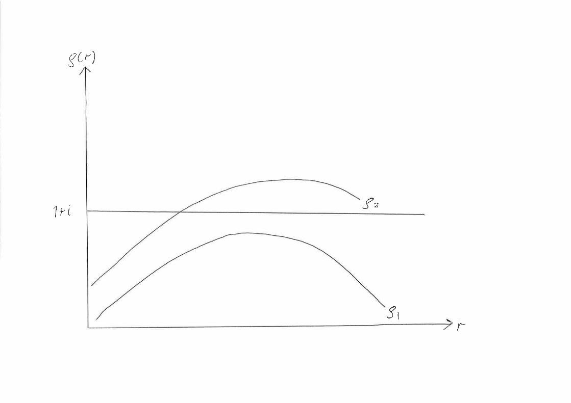
Effects of an overall fall in firms’equity

• Situation with three borrower groups as in graph a1 < a2 < a3Initially Group 3 and 2 all receive credit, Group 1 is rationed, all of themdenied credit.

• If a falls in all three groups: Group 2 also get rationed (not consideredcreditworthy anymore) and do not invest. Interest rate on loans for group3 increases; not rationed, but fewer borrowers in group 3 demand creditand carry out investments.

Example of a pecuniary externality impacting the real economy.

• Firms fail and their banks sell their assets in a fire-sale. Price of theseassets drop. Solvent firms holding similar assets, have their net value, i.e.,their equity, lowered. With imperfect credit markets like in this model,some of the firms may not be able to borrow anymore, others still receivecredit but at higher interest rate. Fewer investment projects carried out.I.e., pecuniary externality from banks’fire sale has real economic impact.