ECON 385. IntermediateMacroeconomic Theory II. Solow

Model With Technological Progressand Data

Instructor: Dmytro Hryshko

1 / 35

Examples of technological progress

1970: 50,000 computers in the world; 2000:51% of U.S. households have 1 or morecomputers

The real price of computer power has fallenan average of 30% per year over the pastthree decades

The average car built in 1996 contained morecomputer processing power than the firstlunar landing craft in 1969

1981: 213 computers connected to theInternet; 2000: 60 million computersconnected to the Internet

2 / 35

Technological progress in the Solow model

A new variable: E = labour efficiency

Assume technological progress islabour-augmenting—it increases labourefficiency at the exogenous rate g:

∆E

E= g

3 / 35

We now write the production function as

Y = F (K,EL)

where L× E = the number of effectiveworkers (efficient units of labour).

Hence, increases in labour efficiency have thesame effect on output as increases in thelabour force.

4 / 35

Notation

y = YEL = output per effective worker

k = KEL = output per effective worker

Production function per effective worker:y = f(k)

Saving and investment per effective worker:sy = sf(k)

5 / 35

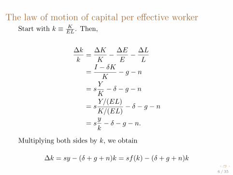
The law of motion of capital per effective workerStart with k ≡ K

EL . Then,

∆k

k=

∆K

K− ∆E

E− ∆L

L

=I − δK

K− g − n

= sY

K− δ − g − n

= sY/(EL)

K/(EL)− δ − g − n

= sy

k− δ − g − n.

Multiplying both sides by k, we obtain

∆k = sy − (δ + g + n)k = sf(k) − (δ + g + n)k

6 / 35

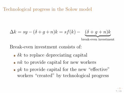
Technological progress in the Solow model

∆k = sy− (δ+ g+n)k = sf(k)− (δ + g + n)k︸ ︷︷ ︸break-even investment

Break-even investment consists of:

δk to replace depreciating capital

nk to provide capital for new workers

gk to provide capital for the new “effective”workers “created” by technological progress

7 / 35

8 / 35

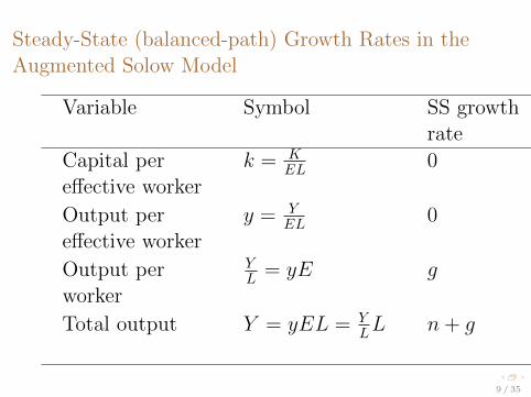
Steady-State (balanced-path) Growth Rates in theAugmented Solow Model

Variable Symbol SS growthrate

Capital per k = KEL 0

effective worker

Output per y = YEL 0

effective worker

Output per YL = yE g

worker

Total output Y = yEL = YLL n+ g

9 / 35

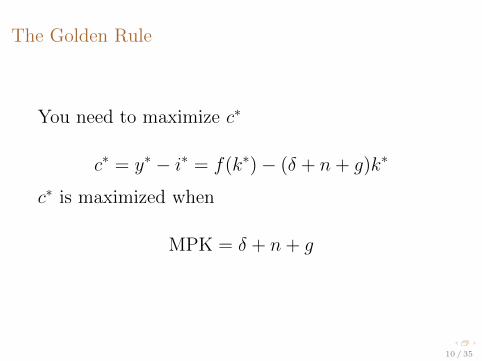
The Golden Rule

You need to maximize c∗

c∗ = y∗ − i∗ = f(k∗) − (δ + n+ g)k∗

c∗ is maximized when

MPK = δ + n+ g

10 / 35

Policies to promote growth

Are we saving enough? Too much?

What policies might change the saving rate?

How should we allocate our investmentbetween privately owned physical capital,public infrastructure, and “human capital”?

What policies might encourage fastertechnological progress?

11 / 35

Evaluating the Rate of Saving

Use the Golden Rule to determine whetherour saving rate and capital stock are too high,too low, or about right.

To do this, we need to compare (MPK −δ) to(n+ g).

If (MPK −δ) > (n+ g), then we are belowthe Golden Rule steady state and shouldincrease s.

If (MPK −δ) < (n+ g), then we are above theGolden Rule steady state and should reduce s.

12 / 35

Policies to increase the saving rate

Increase incentives for private saving:

reduce capital gains tax, corporate incometax, estate tax as they discourage saving

replace income tax with a consumption tax

improve incentives for retirement savingsaccounts

13 / 35

Allocating the economy’s investment

In the Solow model, there’s one type of capital

In the real world, there are many types, whichwe can divide into three categories:–private capital stock–public infrastructure–human capital: the knowledge and skills thatworkers acquire through education

How should we allocate investment amongthese types?

14 / 35

Allocating the economy’s investment

Equalize tax treatment of all types of capitalin all industries, then let the market allocateinvestment to the type with the highestmarginal product.

Industrial policy: Government should activelyencourage investment in capital of certaintypes or in certain industries, because theymay have positive externalities (by-products)that private investors don’t consider.

15 / 35

Encouraging technological progress

Patent laws: encourage innovation bygranting temporary monopolies to inventorsof new products

Tax incentives for R&D

Grants to fund basic research at universities

Industrial policy: encourage specific industriesthat are key for rapid technological progress

16 / 35

Growth empirics: Solow model against the facts

Solow model’s steady state exhibits balancedgrowth—many variables grow at the samerate

Solow model predicts Y/L and K/L grow atsame rate (g), so that K/Y should beconstant. True in the real world.

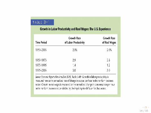
Solow model predicts real wage grows at samerate as Y/L, while real rental price isconstant. True in the real world. Table

17 / 35

18 / 35

Predictions and Empirics

If the world behaves like the Solow model, weshould observe convergence (in incomes percapita) if countries differ only with respect toinitial capital and share same s, n, δ

. . . then poor countries should grow faster(since they’re farther away from SS) and wewould expect a negative relationship betweeninitial income and growth

Do not observe such absolute convergence in abroad cross-section of countries as they differin s, n and δ

19 / 35

.16 Chapter 1 Economic Growth and Economic Development: The Questions

Average growth rate of GDP, 1960–2000

0.06

0.04

0.02

0.00

–0.02

TWN

CHN GNQ KOR

HKG

THA MYS ROM JPN SGP

IRL

LKA LUX

GHA LSO PAK

PRT ESP AUT

IND GRC IDN CPV MUS ISRBELEGY ITA

TUR FRAMAR FIN NOR

PANSYR

DOM GBR MWI NPL

BRA ISL

DNK USA

GAB NLD

TZA CIV PHL PRY IRN CHL

TTO SWE

CANCHE

ETH AUS GNB

BFA BEN COL MEX BRBZWE ECU ZAF

URY GMB COG CRI ARGMLI CMR GTMMOZ

UGA DZA NZL

HND BOL SLV BDI

ZMB NGA PER

TGO KEN JAMRWA COM SEN

GIN VEN

TCD JOR NER

MDG NIC

7 8 9 10 11 Log GDP per worker, 1960

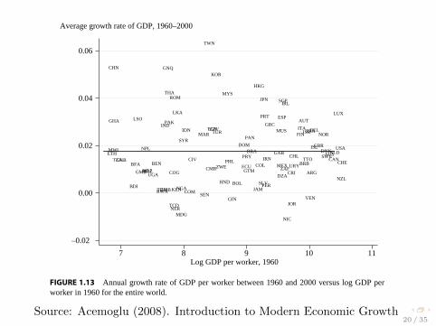
FIGURE 1.13 Annual growth rate of GDP per worker between 1960 and 2000 versus log GDP per worker in 1960 for the entire world.

is an error term capturing all other omitted factors. The variables in X are included because they are potential determinants of steady-state income and/or growth. First note that without covariates, (1.1) is quite similar to the relationship shown in Figure 1.9. In particular, since gi,t,t−1 ≈ log yi,t − log yi,t−1, (1.1) can be written as

log yi,t ≈ (1 + α) log yi,t−1 + εi,t .

Figure 1.9 showed that the relationship between log GDP per worker in 2000 and log GDP per worker in 1960 can be approximated by the 45◦ line, so that in terms of this equation, α should be approximately equal to 0. This observation is confirmed by Figure 1.13, which depicts the relationship between the (geometric) average growth rate between 1960 and 2000 and log GDP per worker in 1960. This figure reiterates that there is no “unconditional” convergence for the entire world—no tendency for poorer nations to become relatively more prosperous—over the postwar period.

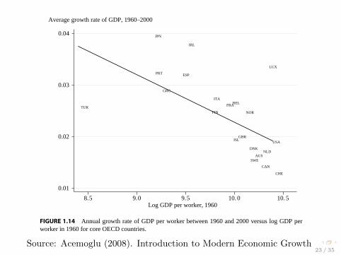
While there is no convergence for the entire world, when we look among the member nations of the Organisation for Economic Co-operation and Development (OECD),2 we see a different pattern. Figure 1.14 shows that there is a strong negative relationship between log GDP per worker in 1960 and the annual growth rate between 1960 and 2000. What distinguishes this sample from the entire world sample is the relative homogeneity of the OECD countries, which

2. “OECD” here refers to the members that joined the OECD in the 1960s (this excludes Australia, New Zealand, Mexico, and Korea). The figure also excludes Germany because of lack of comparable data after reunification.

Source: Acemoglu (2008). Introduction to Modern Economic Growth20 / 35

Convergence

Many poor countries do NOT grow fasterthan rich ones. Does this mean the Solowmodel fails?

No, because “other things” aren’t equal.

In samples of countries with similar savings &population growth rates, income gaps shrinkabout 2%/year

21 / 35

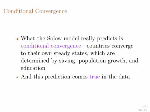
Conditional Convergence

What the Solow model really predicts isconditional convergence—countries convergeto their own steady states, which aredetermined by saving, population growth, andeducation

And this prediction comes true in the data

22 / 35

1.5 Conditional Convergence . 17

Average growth rate of GDP, 1960–2000

AUS

BEL

CAN

DNK

FIN

FRA

GRC

ISL

IRL

ITA

JPN

LUX

NLD

NOR

PRT ESP

SWE

CHE

TUR

GBR

USA

0.01

0.02

0.03

0.04

8.5 9.0 9.5 10. 0 10. 5 Log GDP per worker, 1960

FIGURE 1.14 Annual growth rate of GDP per worker between 1960 and 2000 versus log GDP per worker in 1960 for core OECD countries.

have much more similar institutions, policies, and initial conditions than for the entire world. Thus there might be a type of conditional convergence when we control for certain country characteristics potentially affecting economic growth.

This is what the vector X captures in (1.1). In particular, when this vector includes such variables as years of schooling or life expectancy, using cross-sectional regressions Barro and Sala-i-Martin estimate α to be approximately −0.02, indicating that the income gap between countries that have the same human capital endowment has been narrowing over the postwar period on average at about 2 percent per year. When this equation is estimated using panel data and the vector X includes a full set of country fixed effects, the estimates of α become more negative, indicating faster convergence.

In summary, there is no evidence of (unconditional) convergence in the world income distribution over the postwar era (in fact, the evidence suggests some amount of divergence in incomes across nations). But there is some evidence for conditional convergence, meaning that the income gap between countries that are similar in observable characteristics appears to narrow over time. This last observation is relevant both for recognizing among which countries the economic divergence has occurred and for determining what types of models we should consider for understanding the process of economic growth and the differences in economic performance across nations. For example, we will see that many growth models, including the basic Solow and the neoclassical growth models, suggest that there should be transitional dynamics as economies below their steady-state (target) level of income per capita grow toward that level. Conditional convergence is consistent with this type of transitional dynamics.

Source: Acemoglu (2008). Introduction to Modern Economic Growth23 / 35

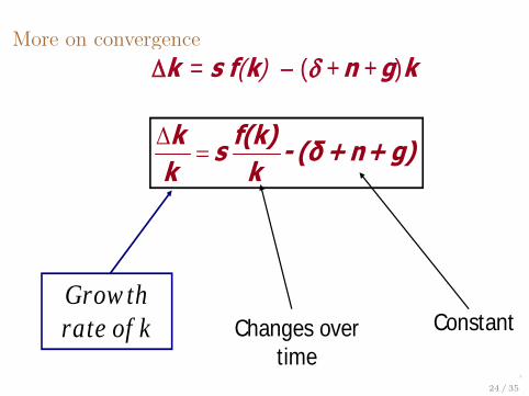
More on convergence

Lecture 16 Growth V slide 3

Solow Model and Convergence

k = s f(k) ( +n +g)k

k f(k)s - (δ+ n+ g)k k

Growth rate of k Changes over

timeConstant

24 / 35

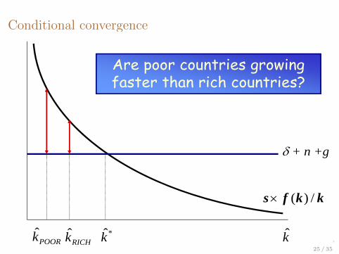
Conditional convergence

Lecture 16 Growth V slide 4

Growth Rate Graph

+ n +g

*k̂POORk̂ RICHk̂ k̂

( ) /s f k k

Are poor countries growingfaster than rich countries?

25 / 35

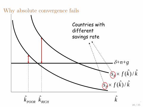
Why absolute convergence fails

Lecture 16 Growth V slide 7

Convergence

+n+g

POORk̂ RICHk̂ k̂

kkfsPˆ/)ˆ(

kkfsRˆ/)ˆ(

Countries with different savings rate

26 / 35

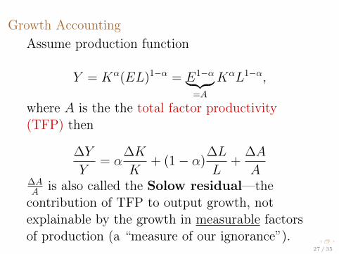
Growth Accounting

Assume production function

Y = Kα(EL)1−α = E1−α︸ ︷︷ ︸=A

KαL1−α,

where A is the the total factor productivity(TFP) then

∆Y

Y= α

∆K

K+ (1 − α)

∆L

L+

∆A

A∆AA is also called the Solow residual—the

contribution of TFP to output growth, notexplainable by the growth in measurable factorsof production (a “measure of our ignorance”).

27 / 35

Growth Accounting

Solow (1957): developed the growthaccounting framework and applied to U.S.data for assessment of the sources of growthduring the early 20th century.

Conclusion: a large part of of the growth wasdue to technological progress (growth inTFP)!

28 / 35

Table 8-3 Accounting for Economic Growth in Canada

Mankiw and Scarth: Macroeconomics, Canadian Fifth Edition

Copyright © 2014 by Worth Publishers

29 / 35

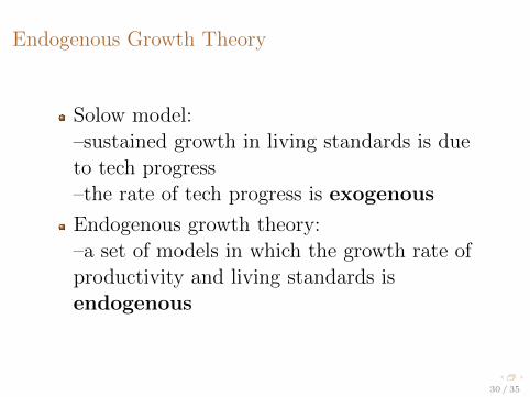
Endogenous Growth Theory

Solow model:–sustained growth in living standards is dueto tech progress–the rate of tech progress is exogenous

Endogenous growth theory:–a set of models in which the growth rate ofproductivity and living standards isendogenous

30 / 35

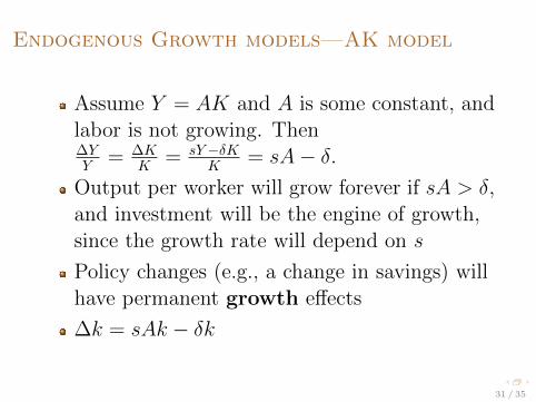
Endogenous Growth models—AK model

Assume Y = AK and A is some constant, andlabor is not growing. Then∆YY = ∆K

K = sY−δKK = sA− δ.

Output per worker will grow forever if sA > δ,and investment will be the engine of growth,since the growth rate will depend on s

Policy changes (e.g., a change in savings) willhave permanent growth effects

∆k = sAk − δk

31 / 35

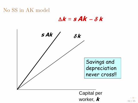
No SS in AK model

Lecture 16 Growth V slide 17

No steady state

k = s Ak k

Capital per worker, k

ks Ak

Savings and depreciation never cross!!

32 / 35

No convergence in AK model

Lecture 16 Growth V slide 19

No Convergence

POORk RICHk k

s A

33 / 35

Important insight of AK models—sustainedgrowth in output can be generated by theeconomy’s fundamentals (A and s).

Important feature of the production functionthat generates sustained growth—the returnsto capital are constant, not diminishing.But...is it a reasonable assumption?

34 / 35

No, if “capital” is narrowly defined (plantsand equipment)

Maybe yes with with a broad definition of“capital” (physical and human capital,knowledge)

35 / 35