econ 325: introduction to empirical...

Econ 325: Introduction to

Empirical Economics

Lecture 7

Estimation: Single Population

Copyright © 2010 Pearson Education, Inc. Publishing as Prentice Hall Ch. 7-1

Parameters

� A parameter is some constant that summarizes

the feature of population distribution.

� Examples

� � population mean

� �� population variance

� � population fraction

� We often use � (``theta’’) to denote a parameter


Estimation problem

� Given a sample, we would like to make our best

guess about a parameter of interest.

� Examples:

� Sample mean �� is our guess of population mean �� Sample variance � is our guess of population

variance ��

� Sample fraction �̂ is our guess of population fraction �


Point Estimator

� A point estimator of a population parameter � is

a function of random sample:

�� = ��(��, ��, … , ��)� Example:

�� = �� , ��, … , �� ≡ �� ∑ ��

� A specific realized value of that random variable

is called an point estimate.


7.1

Unbiasedness

� A point estimator is said to be an

unbiased estimator of the parameter θθθθ if the

expected value, or mean, of the sampling

distribution of is θθθθ,

� Examples:

� The sample mean is an unbiased estimator of μ

� The sample variance s2 is an unbiased estimator of σ2

� The sample proportion is an unbiased estimator of P

θ̂

θ̂

θ)θE( =ˆ


x

p̂

Unbiasedness

� is an unbiased estimator, is biased:

1θ̂ 2θ̂

θ̂θ

1θ̂ 2θ̂

(continued)


Bias

� Let be an estimator of θθθθ

� The bias in is defined as the difference

between its mean and θθθθ

� The bias of an unbiased estimator is 0

θ̂

θ̂

θ)θE()θBias( −= ˆˆ


Example of Biased Estimator

� Given a random sample of n = 2, consider an

estimator for �:

�� = �� + �

� ��

Bias = E �� − � = E[�

� ��] + E[�� ] − �

= �� + �

� � − � = − ��


Clicker Question 7-1

� Given a random sample {��, ��, … , ��}, consider

an estimator for �:

�� = ��This estimator only uses the first observation and

ignores {��, … , ��}. Is this an unbiased estimator?

A). Yes, it is an unbiased estimator.

B). No, it is not an unbiased estimator.



� Given a random sample of n = 2, consider two

estimators for �:

(i) �� = �� + �� and (ii) �� = �

�� + � ��

A). (i) is unbiased but the bias of (ii) is not zero.

B). The bias of (i) not zero but (ii) is unbiased.

C). Both are unbiased.


Efficiency

� We prefer the estimator with the smaller variance.

� Let and be two unbiased estimators of θθθθ.

� Then,

is said to be more efficient than if

The most efficient unbiased estimator of θθθθ is the unbiased estimator with the smallest variance.

)θVar()θVar( 21ˆˆ <

1θ̂ 2θ̂

1θ̂ 2θ̂


Example

� Given a random sample of n = 2 with !"# �� =� �, consider two estimators for �:

�� = �� + �� and �� = ��

� !"#(��) = $%

% !"#(��)+$%

% !"# �� = & '�

� !"#(��) = !"#(��) = � �

� �� is more efficient than �� because !"# �� <!"#(��)


Worksheet Question 1

� In the U.S. presidential election,

� = the population fraction of Trump

supporters

�̂� = the sample fraction of Trump supporters

in random sample of $) voters.

�̂� = the sample fraction of Trump supporters

in random sample of $)))) voters.

Compute the variance of �̂� and �̂�.



� Given a random sample of n = 2, consider two

estimators for �:

�� = �� + �� and �� = �

�� + � ��

Which estimator is more efficient?

A). �� = �� + ��

B). �� = � �� + �

��C). Both are equally efficient.



� Given a random sample of n = 2, consider an

estimator of �:

�* = +�� + (1 − +)��

What is the value of + that gives the smallest

variance of �* ?


Sample average as the most

efficient unbiased estimator

� Given a random sample of n observations,

consider an estimator of �:

�* = ∑ -�� with ∑ -� = 1��

What is the value of {-�}�� that gives the smallest

variance of �* ?


Consistency

� A point estimator �� is said to be a consistent

estimator of � if �� converges in probability to

�, i. e. ,�� 1→ �

� By the Law of Large Numbers, the sample

mean �� is a consistent estimator of � because

��1→ �.


Example


� = the population fraction of voters who

support Trump

�̂ = the sample fraction of voters who

support Trump in random sample of 3voters.

As 3 → ∞, 56 → 5 in probability.



� Consider the following estimator of � = 7[�]:

�� = 18 9 ��

�

��

A). �� is a consistent estimator of �B). �� is not a consistent estimator of �




�� = 18 − 1 9 ��

�

��

A). �� is a consistent estimator of �B). �� is not a consistent estimator of �




�� = 18 − 1 9 ��

�

��

A). �� is an unbiased estimator of �B). �� is not an unbiased estimator of �


Unbiasedness vs. Consistency

� Consistency is a property of an estimator

when 3 → ∞. Consistency is the result of the

Law of Large Numbers.

� Unbiasedness is a property of an estimator

when 3 is fixed. It is nothing to do with the Law

of Large Numbers.


Another Example

� Consider two estimators of population variance:

�= $3:$ ∑ �� − ��

�*� = $3 ∑ �� − ��

� 7[�] = �� but E �*� = �:�� < ��

� � 1→ �� and �*� 1→ �� as 8 → ∞


Point and Interval Estimates

� A point estimate is a single number,

� a confidence interval provides additional information about variability

Point Estimate

Lower

Limit (L)

Upper

Limit (U)

Width of confidence interval


Confidence Interval Estimate

� An interval gives a range of values

� Based on observation from 1 sample

� The lower limit (L) and upper limit (U) are functions of the sample, e.g.,

; <(��, ��, … , �� < � < =(��, ��, … , ��)) = 0.95


Confidence Interval and Confidence Level

� If P(L < θθθθ < U) = 1 - αααα then the interval from L to U is called a 100(1 - αααα)% confidence interval of θθθθ.

� The quantity (1 - αααα) is called the confidence level of the interval (αααα between 0 and 1)

� From repeated samples, 100(1 - αααα)% of all the confidence intervals will contain the true parameter


2016 Presidential Election: Ohio


General Formula

� The general formula for all confidence

intervals is:

� Example

; �� − 1.96 &�B < � < �� + 1.96 &

�B = 0.95

Point Estimate ±±±± (Reliability Factor)(Standard Error)


How to obtain confidence

intervals for ?

; −1.96 < �� − �� 8B⁄ < 1.96 = 0.95

↔ ; −1.96 �8B < �� − � < 1.96 �

8B = 0.95

↔ ; �� − 1.96 �8B < � < �� + 1.96 �

8B = 0.95



intervals for p?

; −1.96 < �̂ − ��(1 − �) 8⁄B < 1.96 = 0.95

↔ ; −1.96 �(1 − �)8

B < �* − � < 1.96 �(1 − �)8

B = 0.95

↔ ; �* − 1.96 1(�:1)�

B < � < �* + 1.96 1(�:1)�

B = 0.95


Example


� = the population fraction of voters who

support Clinton

�̂ = the sample fraction of voters who

support Clinton

� 95 percent confidence interval is given by

�̂ − 1.96 �̂(1 − �̂)8

B< � < �̂ + 1.96 �̂(1 − �̂)

8B


Example

� On Oct 24 of 2016, the survey was conducted

in Florida after the final presidential debate.

� Among 1166 likely registered voters, who

support either Clinton or Trump, there are 602

Clinton voters and 564 Trump voters.

� What is the 95 percent confidence interval for

the population fraction of Trump voters?

� P(0.455 < p < 0.512) = 0.95



� Suppose that, among randomly sampled

8 registered voters, the sample fraction of

Trump supporter is 51.6 percent. What will

happen to the 95 percent confidence interval

when 8 → ∞?

A). The confidence interval diverges to [−∞, ∞].B). The confidence interval converges to the

population fraction of Trump supporter.


Confidence Intervals

Population Mean

σ2 Unknown

ConfidenceIntervals

PopulationProportion

σ2 Known


PopulationVariance

Confidence Interval for μ(σ2 Known)

� Assumptions

� Population variance σ2 is known

� Population is normally distributed

� If population is not normal, use large sample

� Confidence interval estimate:

(where zα/2 is the normal distribution value for a probability of α/2 in each tail)

n

σzxμ

n

σzx α/2α/2 +<<−


7.2

Finding the Reliability Factor, zα/2

� Consider a 95% confidence interval:

z = -1.96 z = 1.96

.951 =α−

.0252

α= .025

2

α=

Point EstimateLower Limit

UpperLimit

Z units:

X units: Point Estimate

0

� Find z.025 = ±±±±1.96 from the standard normal distribution table


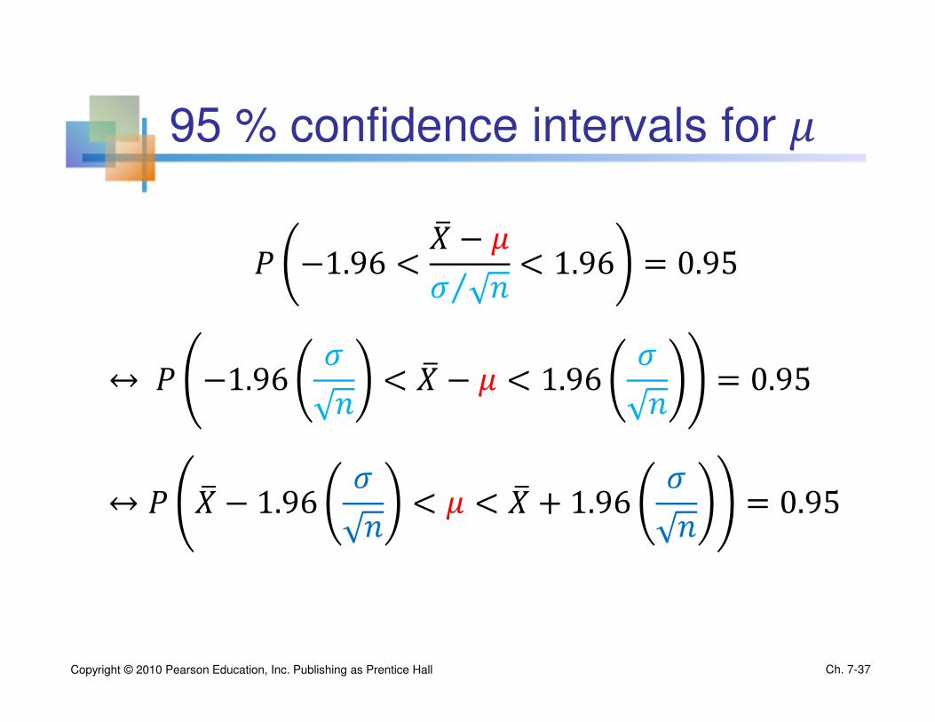
95 % confidence intervals for

; −1.96 < �� − �� 8B⁄ < 1.96 = 0.95

↔ ; −1.96 �8B < �� − � < 1.96 �

8B = 0.95

↔ ; �� − 1.96 �8B < � < �� + 1.96 �

8B = 0.95


Common Levels of Confidence

� Commonly used confidence levels are 90%,

95%, and 99%

Confidence

Level

Confidence

Coefficient, Zαααα/2 value

1.28

1.64

1.96

2.33

2.58

3.08

3.27

.80

.90

.95

.98

.99

.998

.999

80%

90%

95%

98%

99%

99.8%

99.9%

α−1



; �� − E �8B < � < �� + E �

8B = 0.90

What is the value of z ?

A). z = 1.64

B). z = 1.96

C). z = 2.58


90 % confidence intervals for

; −1.64 < �� − �� 8B⁄ < 1.64 = 0.90

↔ ; −1.64 �8B < �� − � < 1.64 �

8B = 0.90

↔ ; �� − 1.64 �8B < � < �� + 1.64 �

8B = 0.90


Intervals and Level of Confidence

μμx

=


Intervals extend from

to

100(1-α)%of intervals constructed contain μ;

100(α)% do

not.

Sampling Distribution of the Mean

n

σzxL −=

n

σzxU +=

x

x1

x2

/2α /2αα−1



Given a realized sample, the confidence interval

computed from the sample contains the

population parameter with probability either one

or zero.

A). True

B). False


Example


in Wisconsin. Among 1079 likely registered

voters who support either Trump or Clinton,

there are 502 Trump voters and 577 Clinton

voters.

� The 95% confidence interval for the population

fraction of Trump voters:

[0.454 , 0.494]

� On Nov 8, 50.5% voted for Trump: p = 0.505


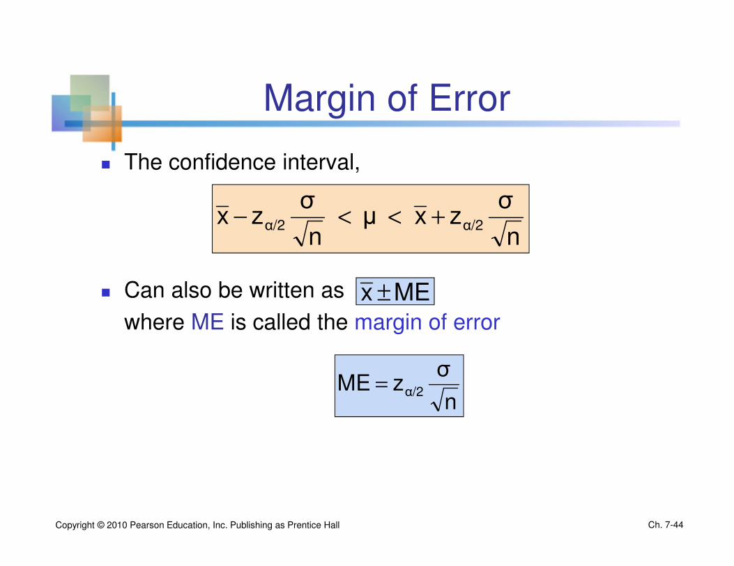
Margin of Error

� The confidence interval,

� Can also be written as

where ME is called the margin of error

n

σzxμ

n

σzx α/2α/2 +<<−

MEx ±

n

σzME α/2=


Post-ABC Tracking Poll: Clinton 47, Trump 43 on election eve

``The poll finds 47 percent of likely voters support Clinton while 43 percent

support Trump.’’

``Clinton’s edge in the Post-ABC poll

does not reach statistical significance given the poll’s 2.5 percentage-point margin in sampling error around each candidate’s support.’’


Reducing the Margin of Error

The margin of error can be reduced if

� the population standard deviation can be reduced (σ↓)

� The sample size is increased (n↑)

� The confidence level is decreased, (1 – α) ↓

n

σzME α/2=


Example

� A sample of 27 light bulb from a large

normal population has a mean life length of

1478 hours. We know that the population

standard deviation is 36 hours.

� Determine a 95% confidence interval for the

true mean length of life in the population.


Example

� Solution:

x ± zσ

n

=1478 ± 1.96 (36/ 27)

=1478 ± 13.58

1464.42 < µ < 1491.58

(continued)


Interpretation

� We are 95% confident that the true mean

life time is between 1464.42 and 1491.58

� Although the true mean may or may not be

in this interval, 95% of intervals formed in

this manner will contain the true mean





1500 hours. We know that the population

standard deviation is 10 hours.







1500 hours. We don’t know the population

standard deviation but the sample standard deviation is 10 hours.





Population Mean

σ2 Unknown

ConfidenceIntervals


σ2 Known


PopulationVariance

7.3

Confidence Interval for

population mean

; �� − 1.96 �8B < � < �� + 1.96 �

8B = 0.95

Usually, the value of G is not known.

→ Replace G with its estimator:

H = $3 − $ 9(IJ − IK )%

3

J�$

B


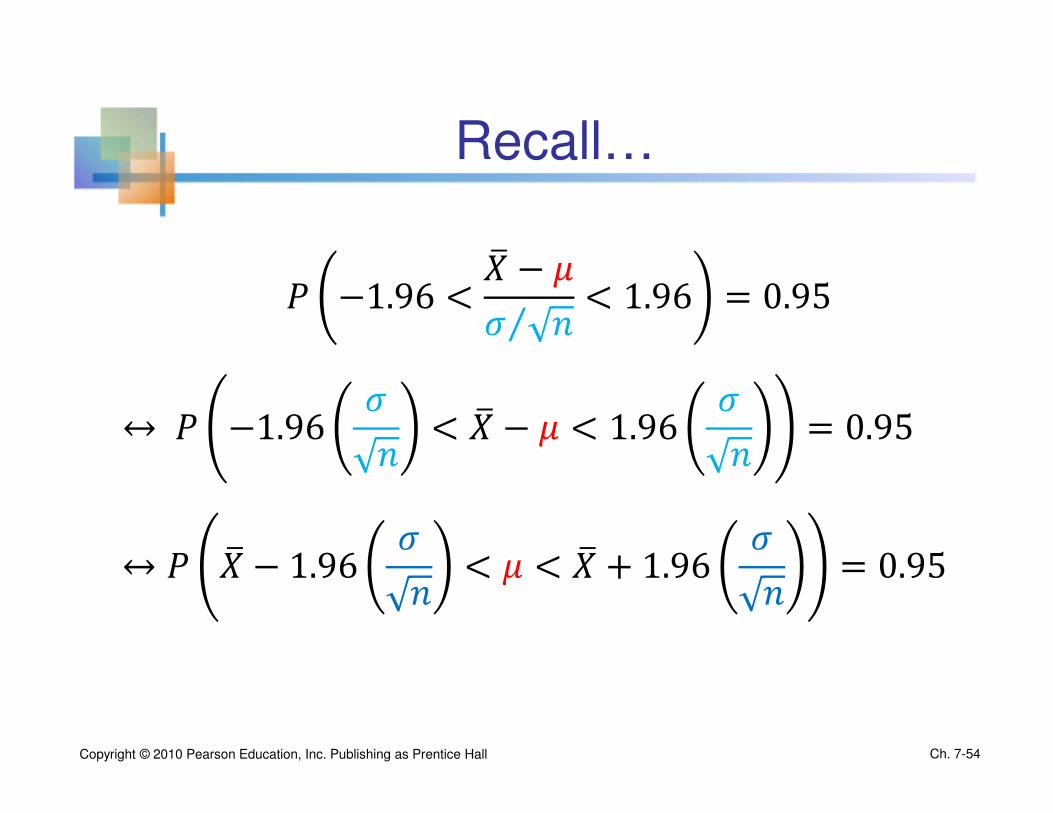
Recall…

; −1.96 < �� − �� 8B⁄ < 1.96 = 0.95

↔ ; −1.96 �8B < �� − � < 1.96 �

8B = 0.95

↔ ; �� − 1.96 �8B < � < �� + 1.96 �

8B = 0.95


Confidence interval

when is not known

� If 8 is large,

; �� − 1.96 8B < � < �� + 1.96

8B ≈ 0.95

� If 8 is small,

; �� − 1.96 8B < � < �� + 1.96

8B < 0.95

→ 1.96 has to be replaced with something larger!


Confidence interval

We need to find the value of M such that

; −M < �� − � 8B⁄ < M = 0.95

→ What is the distribution of T�:UV �B⁄ ?


Student’s t Distribution

� Consider a random sample of n observations

from a normally distributed population

� Then, the random variable

follows the Student’s t distribution with (n - 1) degrees of freedom (d.f.)

ns/

μxt

−=



W = �� − � 8B⁄

=XKYZ[ \B⁄

\Y] ^' [' (�:�)_B

= `ab' c⁄B -dWe f = 8 − 1



Let g~i(0,1) and χc� follows Chi-square

distribution with degrees of freedom f. Then, a

random variable

Wc = `ab' c⁄B

follows Student’s t distribution with degrees of

freedom f.



t0

t (df = 5)

t (df = 13)t-distributions are bell-shaped and symmetric, but have ‘fatter’ tails than the normal

Standard Normal

(t with df = ∞)

Note: t Z as n increases


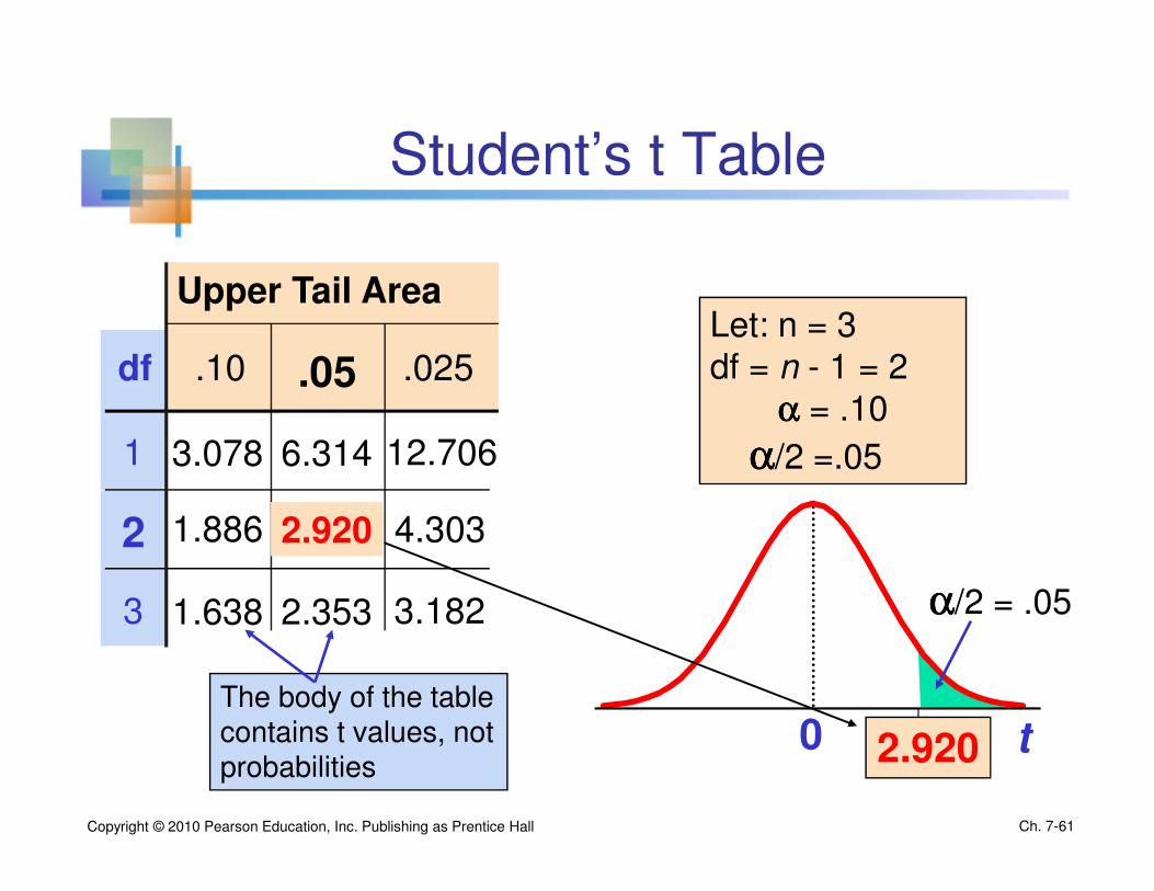
Student’s t Table

Upper Tail Area

df .10 .025.05

1 12.706

2

3 3.182

t0 2.920

The body of the table contains t values, not probabilities

Let: n = 3 df = n - 1 = 2

αααα = .10

αααα/2 =.05

αααα/2 = .05

3.078

1.886

1.638

6.314

2.920

2.353

4.303


t distribution values

With comparison to the Z value

Confidence t t t ZLevel (10 d.f.) (20 d.f.) (30 d.f.) ____

.80 1.372 1.325 1.310 1.282

.90 1.812 1.725 1.697 1.645

.95 2.228 2.086 2.042 1.960

.99 3.169 2.845 2.750 2.576

Note: t Z as n increases



intervals for when n=11?

; −2.228 < �� − � 11B⁄ < 2.228 = 0.95

↔ ; −2.22811B < �� − � < 2.228

11B = 0.95

↔ ; �� − 2.22811B < � < �� + 2.228

11B = 0.95



Given a randomly sampled 11 observations with

mean �, the distribution of T�:U

V ��B⁄ is always given

by t-distribution with the degree of freedom 10.

A). True

B). False


Example

A random sample of n = 25 has x = 50 and s = 8. Form a 95% confidence interval for μ

� d.f. = n – 1 = 24, so

The confidence interval is

2.064tt 24,.025α/21,n ==−

53.302μ46.698

25

8(2.064)50μ

25

8(2.064)50

n

stxμ

n

stx

α/21,-n α/21,-n

<<

+<<−

+<<−





1500 hours. We don’t know the population

standard deviation but the sample standard deviation is 10 hours.





Population Mean

σ2 Unknown

ConfidenceIntervals


σ2 Known


PopulationVariance

7.4

Confidence Intervals for the Population Proportion, p

� By the Central Limit Theorem,

�̂ − � ~ i(0, �1�)where

� The sample analogue estimator of �1 is

(continued)

n

)p(1p ˆˆ −

n

p)p(1σp

−=



intervals for p?

; −1.96 < �̂ − ��(1 − �) 8⁄B < 1.96 = 0.95

↔ ; −1.96 �(1 − �)8

B < �* − � < 1.96 �(1 − �)8

B = 0.95

↔ ; �* − 1.96 1(�:1)�

B < � < �* + 1.96 1(�:1)�

B = 0.95


Confidence Interval Endpoints

� Upper and lower confidence limits for the population proportion are calculated with the formula

� where � zα/2 is the standard normal value for the level of confidence desired

� is the sample proportion

� n is the sample size

n

)p̂(1p̂zp̂p

n

)p̂(1p̂zp̂

α/2α/2

−+<<

−−

p̂


Example

� A random sample of 100 people

shows that 25 are left-handed.

� Form a 95% confidence interval for

the true proportion of left-handers


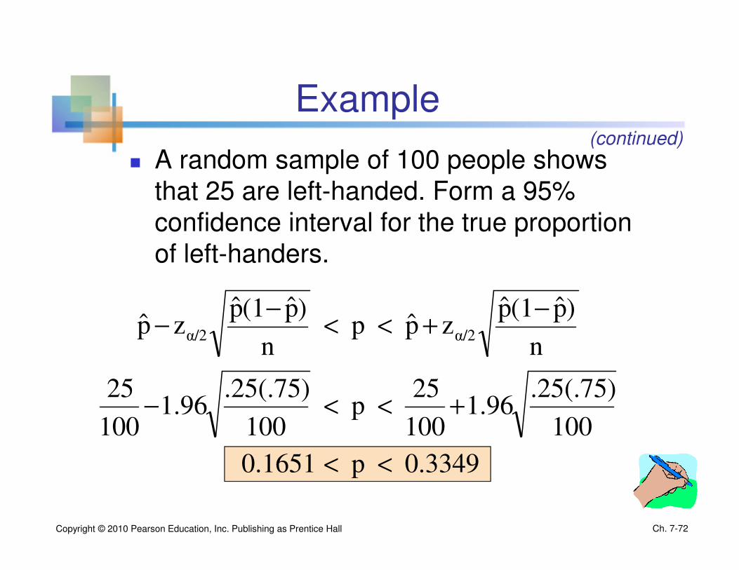
Example

� A random sample of 100 people shows

that 25 are left-handed. Form a 95%

confidence interval for the true proportion

of left-handers.

(continued)

0.3349p0.1651

100

.25(.75)1.96

100

25p

100

.25(.75)1.96

100

25

n

)p̂(1p̂zp̂p

n

)p̂(1p̂zp̂

α/2α/2

<<

+<<−

−+<<

−−


Interpretation

� We are 95% confident that the true percentage of left-handers in the population is between

16.51% and 33.49%.

� Although the interval from 0.1651 to 0.3349 may or may not contain the true proportion, 95% of intervals formed from samples of size 100 in this manner will contain the true proportion.




in Florida after the final presidential debate.

� Among 1166 likely registered voters, who

support either Clinton or Trump, there are 602

Clinton voters and 564 Trump voters.

� What is the 95 percent confidence interval for

the population fraction of Clinton voters?



Population Mean

σ2 Unknown

ConfidenceIntervals


σ2 Known


PopulationVariance

7.5

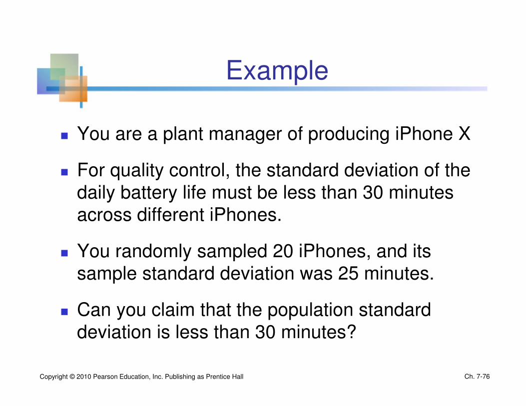
Example

� You are a plant manager of producing iPhone X

� For quality control, the standard deviation of the

daily battery life must be less than 30 minutes

across different iPhones.

� You randomly sampled 20 iPhones, and its

sample standard deviation was 25 minutes.

� Can you claim that the population standard

deviation is less than 30 minutes?



� For a randomly sampled 20 iPhones, the

sample standard deviation of battery lives was

25 minutes.

A). This means that the population standard

deviation is less than 30 minutes for sure.

B). This does not necessarily mean that the

population standard deviation is less than 30

minutes.


Confidence Intervals for the Population Variance

Copyright © 2010 Pearson Education, Inc. Publishing as Prentice Hall

The random variable

2

22

1nσ

1)s(n −=−χ

follows a chi-square distribution with (n – 1)

degrees of freedom when the population is

normally distributed.

(continued)

Ch. 8-78


intervals for �?

; χ�:�,�:k/�� < 8 − 1 �

�� < χ�:�,k/�� = 1 − m

↔ ; 1χ�:�,k/�� < ��

8 − 1 � < 1χ�:�,�:k/�� = 1 − m

↔ ; 8 − 1 �

χ�:�,k/�� < �� < 8 − 1 �

χ�:�,�:k/�� = 1 − m


Confidence Intervals for the Population Variance


The (1 - α)% confidence interval for the

population variance is

2

/2-1 , 1n

22

2

/2 , 1n

2 1)s(nσ

1)s(n

ααχχ −−

−<<

−

(continued)

Ch. 8-80

Example

You are testing the speed of a batch of computer processors. You collect the following data (in Mhz):

Sample size 17Sample mean 3004Sample std dev 74


Assume the population is normal.

Determine the 95% confidence interval for σx2

Ch. 8-81

Finding the Chi-square Values

� n = 17 so the chi-square distribution has (n – 1) = 16 degrees of freedom

� α = 0.05, so use the the chi-square values with area 0.025 in each tail:


probability α/2 = .025

χχχχ216,0.025

χ216

= 28.85

28.85

6.91

2

0.025 , 16

2

/2 , 1n

2

0.975 , 16

2

/2-1 , 1n

==

==

−

−

χχ

χχ

α

α

χχχχ216,0.975= 6.91

probability α/2 = .025

Ch. 8-82


intervals for �?

; 6.91 < (8 − 1) �

�� < 28.85 = 0.95

↔ ; 128.85 < ��

8 − 1 � < 16.91 = 0.95

↔ ; 8 − 1 �

28.85 < �� < 8 − 1 �

6.91 = 0.95


Calculating the Confidence Limits

� The 95% confidence interval is


Converting to standard deviation, we are 95% confident that the population standard deviation of

CPU speed is between 55.1 and 112.6 Mhz

6.91

1)(74)(17σ

28.85

1)(74)(17 22

2 −<<

−

12683σ3037 2 <<

Ch. 8-84

Worksheet Question

For a randomly sampled 20 iPhones, the sample standard deviation of battery lives was 25

minutes. Assume that daily battery life is normally

distributed.

Construct 95 percent confidence interval for the

population standard deviation of battery life.


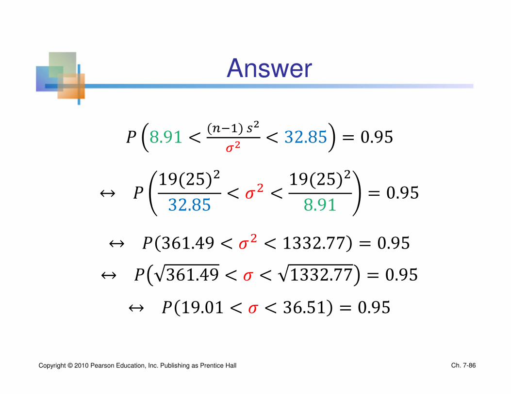
Answer

; 8.91 < (�:�) V'&' < 32.85 = 0.95

↔ ; 19(25)�

32.85 < �� < 19(25)�

8.91 = 0.95

↔ ; 361.49 < �� < 1332.77 = 0.95↔ ; 361.49B < � < 1332.77B = 0.95

↔ ; 19.01 < � < 36.51 = 0.95


econ 325: introduction to empirical...

Documents