Biol2050 1

Ecology Labs. Christopher J. Lortie. York University lortie@yorku.ca

Biol2050 2

Try to see the world as an ecologist and be a Marcovaldo.

The first page from Marcovaldo by Italo Calvino.

Biol2050 3

Purpose of the ecology labs Learning outcomes: The primary objective of the labs is to provide you with experience collecting real, relevant data. Here are the learning outcomes from the activities we conduct in this course. 1. To become familiar with data collection. 2. To be able to analyze data and plot results. 3. To practice and refine scientific writing skills. 4. To be able to approach natural and human systems with an ecological perspective. To realize these objectives we will focus on 3 primary sets of skills. Skills: (1) Data collection, data entry, and data handling. (2) Statistics (t-test, One-way ANOVA, and correlation) and graphs. (3) Scientific paper writing. Activities: The activities or exercises associated with these skills include fieldwork on YorkU campus, exercises in the lab, writing, and a short-test to demonstrate competency and understanding. Products & evaluation: In these labs, you are responsible for generating the following products that will be used to provide feedback via evaluation. Lab quiz. ID samples & short answers on sampling & survey design. 10% Lab report. A publication using data collected in the labs testing a hypothesis. 30% Lab quiz. A quiz in lab to calculate diversity indices. 10%

Biol2050 4

WK1. Eco-Olympics. Location: Meet in the lab, get into groups, but we are going outside to learn sampling techniques. Tasks: Tour campus, visit every major habitat type, and practice techniques including identification of at least 3 different herbs/forbs, 3 different tree species, and 3 bird species. Compare transect versus quadrat versus ring sampling for birds. Then, Eco-olympics competition to ensure that we are all collecting data in the same way for the class. Products: List of common tree, plant, and bird species on campus provided to the teaching assistant by the end of the lab and familiarity with all the different habitats on campus. Description Group work: As groups, practice running transects, setting up quadrats, and doing bird observations. In touring campus, consider the disturbances, management practices, and potential reasons that some sites are meadows, others forest, while others more anthropogenic sites. All have potential ecological function and value and provide habitats for various species – even the more human-impacts locations. This week is your opportunity to look around campus with new eyes and ensure that you know how to sample for the next week. Also start to brainstorm on the variables that you may want to record that either relate to or even cause some of the differences you observe. Transect sampling is best used for plants, seeds, or individuals in general that are dispersed widely at various scales or when you seek to quantify patterns along greater areas. Quadrat sampling is best used for higher resolution data but is more sensitive to location of the sampling and less potential area is sampled (albeit in greater detail). This method does work well for slow moving invertebrates and various other point processes like seeds and plants. Point Counts are used to track changes in breeding bird abundances over time or make comparisons between sites with similar habitats by conducting point counts. Ecologists and ornithologists favor point counts because they are objective, standardized, reputable, and least biased of the methods. They provide us with a comparative index of occurrence, not a complete inventory. Points are laid out at regular intervals along a transect, and the surveyor spends a certain amount of time at each point and records all birds detected during the time period within a specific radius. Transects are also used for birds and imaginary lines drawn through the site to be surveyed (unlike in plant sampling where a tape is used). The surveyor simply follows the transect or transects through the site, recording all birds detected along the way. The surveyor should cover the transect in the same amount of time on each visit. A transect provides a "snapshot", an index of abundance of birds at a site. Skills: 1. Set up a transect in a grassland, forest, human area, and highly disturbed site. Try sampling at various intervals, measuring distance to the nearest plant, and identifying species. 2. Set up a quadrat in each habitat and try again to sample plant abundance and diversity. 3. Set up a 50m point count area (circle that is 50m in diameter) in each habitat and count birds for 5 mins. Try to identify the bird species as well. 4. Use the field guides provided to generate a list of 3 of the most common grass/herb/forb species, trees, and birds and provide to the teaching assistant. Resources: 1. Thompson, K., Austin, K. C., Smith, R. M., Warren, P. H., Angold, P. G. and Gaston, K. J. 2003. Urban domestic gardens (I): putting small-scale plant diversity in context. Journal of Vegetation Science 14: 71-78. 2. Sperling, C.D., and C.J. Lortie. 2010. The importance of urban backgardens on plant and invertebrate recruitment: a field microcosm experiment. Urban Ecosystems 13: 223-235. 3. Marcheselli, M. 2002. Assessing the biotic distance between groups of biological populations by means of replicated counts. Environmetrics 13: 215-223.

Biol2050 5

WK1. Summary of this lab and timeline. 230-3pm. Get equipment and get into the groups assigned by the teaching assistant. 3-4pm. Teaching assistant will explain equipment and demonstrate the sampling techniques. 4-430pm. Practice in your groups each of the sampling techniques. 430-530pm. Eco-Olympics. Competition between groups in sampling techniques. The big picture is that sampling natural systems in a structured repeatable way is critical for ecologists. We need to understand patterns in diversity, structure, and composition of systems before we can effectively manage them or infer important processes that make them look and function the way they do. This is the most important set of skills necessary for research. In the following 3 weeks, you will do one set of sampling techniques per week in each of the three major habitat types on campus. For instance, next week you will do ALL the plant sampling for the large dataset at once in forests, grasslands, and human open-space areas. Then, the week after that you will do invertebrate sampling, and then in the final week you will do animals including birds, squirrels, etc. This will provide us with the means to contrast the three habitat types to infer whether some spots are better for certain organisms relative to other on campus. This will also provide insights into whether we can manage these spaces more effectively as a large, integrated university campus. To summarize, starting next week for three weeks you sample one of the target taxa in 3 woodlots, 3 grasslands, and 3 human open-spaces. This week, you learn the techniques and begin to hone your identification skills.

Biol2050 6

Campus map Insert campus map here. As you can see, there are four small woodlots on campus. Two of these woodlots are impacted by the TTC subway extension. Boyer’s Woodlot is the most studied on campus and is located just north of Lumbers. However, the woodlot just north of Pond Rd now has a tunnel underneath it. There are several large meadows on campus. The largest is just West of Black Creek and South of the tennis centre. However, there are numerous other meadows or old fields on campus. Finally, there are several other habitats on campus that may be very important to invertebrates, squirrels, and some bird species as they are disturbed with lot’s of food. Let’s also explore and sample these.

Biol2050 7

Quick identification primer for plants on campus. In the following pages, a short list of the common species that you will see on campus and a dichotomous tree guide is also included. These lists are based on the plants spotted lurking on campus in the past few years however there will be many, many more. Insert common species list. Pictures Examples of simple dichotomous keys with citation to local field guides.

Biol2050 8

PLANT DATA SHEET TA: Date & Time Last names of group members: Habitat (circle one): forest, grassland, human disturbed open-space Specific name of site: Latitude: Longitude: Elevation TREES - TRANSECT METHOD Length of transect: 25m, Width on either side of the transect 1m Rep (1, 2, or 3) Species (LATIN NAME) # individuals TOTAL

Biol2050 9

PLANT DATA SHEET TA: Date & Time: Last names of group members: Habitat (circle one): forest, grassland, human disturbed open-space Specific site name: Latitude: Longitude: Elevation HERBS/FORBS - QUADRAT SAMPLING Length of transect: 1m X 1m Rep (1, 2, or 3) Species (LATIN NAMES) # of individuals % Cover TOTAL

Biol2050 10

PLANT DATA SHEET TA: Date & Time: Last names of group members: Habitat (circle one): forest, grassland, human disturbed open-space Specific name of site: Latitude: Longitude: Elevation HERBS/FORBS - TRANSECT METHOD Length of transect: 25m (touching transect) Rep (1, 2, or 3) Species (LATIN NAMES) # individuals TOTAL

Biol2050 11

For the bird sampling, you should record the following conditions. BRING WITH YOU TO LABS.

Image from Wikipedia.

Biol2050 12

Common bird species in Toronto Warbler species Yellow Common Yellowthroat Tennessee Chestnut sided Nashville Magnolia Blackburnian Bay breasted Blackpoll Black and white Connecticut Cape May Black throated Blue Yellow rumped Black throated Green American Redstart Ovenbird

List of common birds Cooper's Hawk Northern Mockingbird Baltimore Orioles American Goldfinch American Robins Sharp Shinned Hawks Swainson's Thrush Belted Kingfishers Warbling Red eyed Vireos Cedar Waxwings Black capped Chickadees Gray Catbird Ruby throated Hummingbirds Mourning Doves Blue Jays Northern Cardinals Downy Woodpecker Brown headed Cowbird Red breasted Nuthatch Blue Gray Gnatcatcher Purple Martin Tree Cliff & N. Rough Winged Swallows Chimney Swift Song Sparrow Black Crowned Night Heron Great Blue Heron House Sparrow Rock Pigeon Common Nighthawk Ring Billed Gull & Herring Gull

Fly Catchers Olive sided Yellow bellied Willow/Alder Least Great Crested Eastern Wood Pewee Eastern Kingbird

See field guides for pictures and detailed keys.

Biol2050 13

For the bird sampling, you should do a map of where you spot the birds within the 50m circle. Include important structures or objects that you are within the sampling area. Draw a point, trace where it goes, and label it with a species name.

50m Date & time: Last names of group members: Latitude: Longitude: Habitat (circle the one): forest, grassland, human open-space. Specific name of site: Weather conditions including wind: Total # of birds spotted: Total # of bird species spotted: List of species names: * This same sheet should be used for small mammals you might spot.

Biol2050 14

ANIMAL DATA SHEET TA: Date & Time : Last names of group members : Habitat (circle one) : Forest, Grassland, Human disturbed open-space Specific name of site : Latitude : Longitude : Elevation : Lab Habitat Site Rep Taxa Species name Density Method

Ex lamarque Disturbed Library Lane 1 Aves Branta canadensis 4 Transect

Biol2050 15

Common invertebrate species in Toronto. BRING WITH YOU TO LABS. Major groups Dragonflies and damselflies - Order Odonata - These insects are good indicators of healthy freshwater habitats as they will disappear when water becomes polluted. Adults eat mosquitoes and other insects. Mayflies - order Ephemeroptera - These are small insects that spend most of their lives in the water. Adults emerge in great numbers but live only for a day. Mayflies are an important food source for many fish. Grasshoppers, mantises and crickets - order Orthoptera. Many insects of this order produce sounds by rubbing body parts together. Bugs - order Hemiptera, suborder Homoptera - These are the true bugs; their lower lip is modified into a sucking tube that the insect inserts into plant or animal tissues in order to feed. Aphids and plant hoppers are bugs. Butterflies and moths - order Lepidoptera - These are the familiar beautiful insects that we readily welcome to our gardens. Besides being beautiful to look at, they are important pollinators. Beetles - order Coleoptera - This order includes the familiar June beetle, ladybird beetle and fireflies. Beetles are also pollinators but play an extremely important role in the recycling of animal dung and dead animals. Flies - order Diptera - True flies have a single pair of wings; their hind wings are reduced to stalked knobs called halteres that they use to keep their stability while flying. Flies are important pollinators and also feed on dead carcasses so that nutrients are recycled back into the environment. Ants, wasps and bees - order Hymenoptera - We are all familiar with these insects and often consider them to be a nuisance. However, they are important pollinators of many of our agricultural plants including apples, tomatoes, beans, peas, oilseed and fibre crops. Here are some fantastic digital insect keys. http://www.biology.ualberta.ca/bsc/ejournal/ejournal.html http://www.discoverlife.org/ http://bugguide.net/node/view/15740 All free and online. So, collect samples then look up on laptops/smartphones/tablets.

Biol2050 16

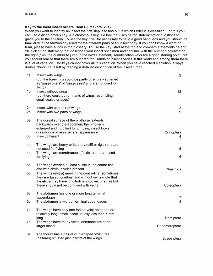
Key to the local insect orders. Hein Bijlmakers. 2012. When you want to identify an insect the first step is to find out in which Order it is classified. For this you can use a dichotomous key. A dichotomous key is a tool that uses paired statements or questions to guide you to the solution. To use the key it will be necessary to have a good hand lens and you should be familiar with the terminology used for the different parts of an insect body. If you don't know a word or term, please have a look in the glossary. To use the key, start at the top and compare statements 1a and 1b. Select the statement that describes your insect specimen and continue with the number indicated on the right (click the number to jump to the next statement). Identification keys are a good starting point, but you should realize that there are hundred thousands of insect species in this world and among them there is a lot of variation. The keys cannot cover all this variation. When you have reached a solution, always double check the result by reading a detailed description of the insect Order. 1a Insect with wings 2 (but the forewings could be partly or entirely stiffened

as 'wing-covers' or 'wing-cases' and are not used for flying)

1b Insect without wings 32 (but there could be remnants of wings resembling

small scales or pads) 2a Insect with one pair of wings 3 2b Insect with two pairs of wings 9 3a The dorsal surface of the prothorax extends

backwards over the abdomen; the hind-legs enlarged and modified for jumping; insect looks grasshopper-like in general appearance Orthoptera

3b Insect different 4 4a The wings are horny or leathery (stiff or rigid) and are

not used for flying 5 4b The wings are membranous (flexible) and are used

for flying 6 5a The wings overlap at least a little in the centre-line

and with obvious veins present Phasmida 5b The wings (elytra) meet in the centre-line (sometimes

they are fused together) and without veins (note that the elytra may have longitudinal grooves or striae but these should not be confused with veins) Coleoptera

6a The abdomen has one or more long terminal

appendages 7 6b The abdomen is without terminal appendages 8 7a The wings have only one forked vein; antennae are

relatively long; small insect usually less than 5 mm long Hemiptera

7b The wings have many veins; antennae are short; larger insect Ephemeroptera

8a The thorax has a pair of club-shaped structures

(halteres) situated just in front of the wings Strepsiptera

Biol2050 17

8b The thorax has a pair of club-shaped structures (halteres) lying just behind the wings (these halteres may be hidden by body hairs and other structures) Diptera

9a The forewings are partly or entirely horny or leathery

and form stiffened covers for the membranous hindwings 10

9b Both pairs of wings are membranous (flexible) and used for flying (sometimes the wings are feather-like rather than membranous or their membranous nature may be obscured by a covering of hairs, scales or waxy powder) 16

10a The mouth-parts form a tube-like 'beak' (rostrum)

which is used for piercing and sucking (this rostrum is usually folded backwards under the body when not in use) Hemiptera

10b The mouth-parts have jaws (mandibles) and are designed for biting and chewing 11

11a The forewings overlap at least a little in the centre-

line and usually with many veins present 12 11b The forewings (elytra) meet in the centre-line and

have no veins (note that the elytra may have longitudinal grooves or striae but these should not be confused with veins) 14

12a The hind-legs are enlarged and modified for jumping;

insect looks like a grasshopper in general appearance Orthoptera

12b The hind-legs are not modified for jumping and are usually similar in thickness to the middle-legs; insect is not grasshopper-like 13

13a The prothorax is much larger than the head; cerci

nearly always many-segmented and fairly prominent Dictyoptera 13b Prothorax and head are of similar size; cerci are not

segmented and very short Phasmida 14a The forewings (elytra) are long and cover all or most

of the abdomen Coleoptera 14b The forewings (elytra) are short and much of the

abdomen remains exposed 15 15a The abdomen has a pair of terminal pincers or

forceps Dermaptera 15b The abdomen has no terminal pincers Coleoptera 16a The wings are very narrow without veins and fringed

with long hairs (feather-like); tarsi are 1- or 2-segmented; small slender insect often found in flowers Thysanoptera

Biol2050 18

16b The wings broader with veins present; if wings are fringed with long hairs then tarsi are comprised of more than 2 segments (the wing veins of some insects may be much reduced and hardly visible or partly obscured by hairs, scales or waxy powder) 17

17a The hindwings are clearly smaller than the forewings 18 17b Both pairs of wings are similar in size or hindwings

larger than forewings 26 18a Wings and much of the body covered with white

waxy powder; tiny insect usually less than 2-3 mm long 19

18b Without powdery covering 20 19a When at rest the wings are held flat over the body;

the mouth-parts form a tube-like 'beak' (rostrum) for piercing and sucking (this rostrum is usually folded backwards under the body when not in use) Hemiptera

19b When at rest the wings are held roof-wise over the body; the mouth-parts have jaws (mandibles) and are designed for biting Neuroptera

20a The wings are more or less covered with very small

scales; the mouth-parts when present are forming a coiled proboscis or 'tongue' Lepidoptera

20b The wings are usually transparent (wings without scales but often hairy); the mouth-parts are not forming a coiled proboscis 21

21a The forewings have many cross-veins making a

network pattern; the abdomen has 2 or 3 long thread-like terminal appendages Ephemeroptera

21b The forewings show relatively few cross-veins; the abdomen is usually without or with only very short terminal appendages (cerci) 22

22a The wings are noticeably covered with hairs; insect

looks moth-like in general appearance Trichoptera 22b The wings are not noticeably hairy (but wings may be

fringed with hairs or tiny surface hairs may be seen if wings are inspected under a microscope or strong hand-lens) 23

23a The mouth-parts form a tube-like 'beak' (rostrum) for

piercing and sucking (usually the rostrum is folded backwards under the body when not in use; the abdomen sometimes has tubular outgrowths or cornicles near the hind end) Hemiptera

23b The mouth-parts has jaws (mandibles) and are designed for biting and chewing 24

24a The tarsi are 4- or 5-segmented; hard-bodied insects

with the abdomen often constricted at its base into a petiole or narrow 'waist' Hymenoptera

Biol2050 19

24b The tarsi are 2- or 3-segmented; small soft-bodied insect 25

25a Antennae with at least 12 segments Psocoptera 25b Antennae with only 9 segments Zoraptera 26a The tarsi are 5-segmented 27 26b The tarsi are 3- or 4-segmented 29 27a The wings are noticeably covered with hairs; insect is

moth-like in general appearance Trichoptera 27b The wings are not noticeably hairy (but tiny hairs

may be seen if the wings are observed under a microscope or with a strong hand-lens) 28

28a The front of the head is extended downwards to form

a beak-like structure with jaws (mandibles) at its tip Mecoptera 28b Insect without such a beak-like extension of the head Neuroptera 29a The tarsi are 4-segmented Isoptera 29b The tarsi are 3-segmented 30 30a The wings are noticeably hairy; the front tarsi are

with the first segment greatly swollen Embioptera 30b The wings are not noticeably hairy; the front tarsi are

simple 31 31a The wings have many cross-veins, which makes a

network pattern; wings are held away from the body at rest (either outstretched or folded vertically); the antennae are short and inconspicuous Odonata

31b The wings have relatively few cross-veins and are folded flat over the body when at rest; the antennae are long and slender (longer than the width of the head) Plecoptera

32a Small soft-bodied insect which lives on terrestrial

plants with the body encased under a protective shield ('scale') or the body is partly covered with white waxy filaments or powder Hemiptera

32b Insect different 33 33a Thoracic legs are absent or enclosed in a membrane

preventing any movement (Larvae and pupae of most Orders of

Endopterygota) 33b Thoracic legs are present and fully functional 34 34a The abdomen has false-legs or prolegs (prolegs are

fleshy leg-like structures that are different from and additional to the jointed legs of the thorax); the insect looks like a caterpillar in general appearance 35

34b The abdomen has no prolegs; the insect is not caterpillar-like in appearance 37

35a Abdomen with not more than 5 pairs of prolegs Larvae of Lepidoptera

Biol2050 20

35b Abdomen has at least 6 pairs of prolegs 36 36a The head has a single small eye (ocellus) on each

side Larvae of Hymenoptera 36b The head has several small eyes (ocelli) on each

side Larvae of Mecoptera 37a The insect lives in a terrestrial habitat or on the

surface of water (not underwater) 38 37b The insect is truly aquatic (living underwater) 70 38a The abdomen has cerci or other terminal

appendages (but be careful not to confuse terminal hairs or bristles with cerci) 39

38b The abdomen does not have such terminal appendages (but it may have small appendages on proximal segments or a pair of tubular outgrowths or cornicles near the hind end) 56

39a The abdomen has 6 or fewer segments; usually the

abdomen has a forked terminal appendage (springing organ) folded under the rear end when not in use Collembola

39b The abdomen has more than 6 segments (usually 8 or more are clearly visible); the terminal appendages are of a different form 40

40a The antennae are short and often inconspicuous (the

same length as the head or shorter) 41 40b The antennae are long and conspicuous (usually

they are much longer than the head) 42 41a The tarsi have at least 3 segments (usually they are

5-segmented) Phasmida 41b The tarsi have fewer than 3 segments (often they are

reduced to single or paired claws on the end of each leg) Larvae of Coleoptera

42a The hind-legs are enlarged and modified for jumping;

insect looks like a grasshopper in general appearance Orthoptera

42b The hind-legs are not modified for jumping; usually the hind-legs are similar in thickness to the middle-legs; insect does not look grasshopper-like 43

43a The terminal appendages of the abdomen form a

pair of pincers or forceps 44 43b The terminal appendages of the abdomen are

different 45 44a The tarsi are 3-segmented Dermaptera 44b The tarsi are 1-segmented Diplura 45a The terminal appendages of the abdomen are long

(much more than half the length of the abdomen) 46

Biol2050 21

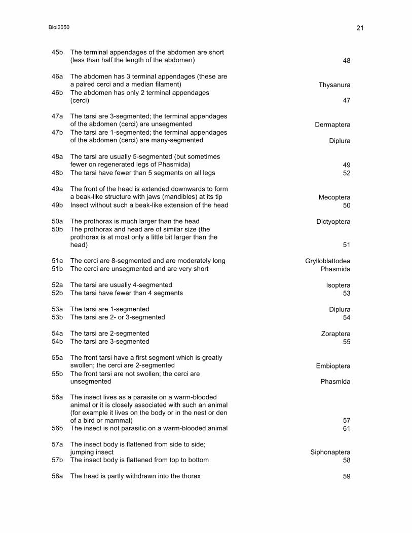
45b The terminal appendages of the abdomen are short (less than half the length of the abdomen) 48

46a The abdomen has 3 terminal appendages (these are

a paired cerci and a median filament) Thysanura 46b The abdomen has only 2 terminal appendages

(cerci) 47 47a The tarsi are 3-segmented; the terminal appendages

of the abdomen (cerci) are unsegmented Dermaptera 47b The tarsi are 1-segmented; the terminal appendages

of the abdomen (cerci) are many-segmented Diplura 48a The tarsi are usually 5-segmented (but sometimes

fewer on regenerated legs of Phasmida) 49 48b The tarsi have fewer than 5 segments on all legs 52 49a The front of the head is extended downwards to form

a beak-like structure with jaws (mandibles) at its tip Mecoptera 49b Insect without such a beak-like extension of the head 50 50a The prothorax is much larger than the head Dictyoptera 50b The prothorax and head are of similar size (the

prothorax is at most only a little bit larger than the head) 51

51a The cerci are 8-segmented and are moderately long Grylloblattodea 51b The cerci are unsegmented and are very short Phasmida 52a The tarsi are usually 4-segmented Isoptera 52b The tarsi have fewer than 4 segments 53 53a The tarsi are 1-segmented Diplura 53b The tarsi are 2- or 3-segmented 54 54a The tarsi are 2-segmented Zoraptera 54b The tarsi are 3-segmented 55 55a The front tarsi have a first segment which is greatly

swollen; the cerci are 2-segmented Embioptera 55b The front tarsi are not swollen; the cerci are

unsegmented Phasmida 56a The insect lives as a parasite on a warm-blooded

animal or it is closely associated with such an animal (for example it lives on the body or in the nest or den of a bird or mammal) 57

56b The insect is not parasitic on a warm-blooded animal 61 57a The insect body is flattened from side to side;

jumping insect Siphonaptera 57b The insect body is flattened from top to bottom 58 58a The head is partly withdrawn into the thorax 59

Biol2050 22

58b The head is not withdrawn into the thorax 60 59a The antennae are short and inconspicuous (they are

much shorter than the head); legs with strong and distinctly hooked tarsal claws Diptera

59b The antennae are long and conspicuous (they are more than twice the length of the head); legs have small and only slightly curved tarsal claws Hemiptera

60a At least the prothorax is distinct from the other

thoracic segments; the legs have small tarsal claws; the mouth-parts have jaws (mandibles) and are designed for biting Mallophaga

60b All the thoracic segments are fused into a single unit; the legs have large tarsal claws which can close tightly against the legs; the mouth-parts form a tube-like proboscis for piercing and sucking (this proboscis is retracted within the head when not in use) Siphunculata

61a Insect without antennae (very small soil-living insects

usually less than 2 mm long) Protura 61b Antennae are present 62 62a The abdomen is strongly constricted at its base into

a narrow petiole or 'waist'; the antennae are often bent into an elbowed shape Hymenoptera

62b The abdomen is not constricted into a 'waist'; the antennae are more or less straight 63

63a The body is covered with dense scales and flattened

hairs Lepidoptera 63b The body is bare or with sparse bristle-like hairs 64 64a The mouth-parts form a tube-like proboscis or

rostrum for piercing and/or sucking (this proboscis is usually folded backwards under the head when not in use) 65

64b The mouth-parts are with jaws (mandibles) and designed for biting and/or chewing 67

65a The tarsi are usually 5-segmented Diptera 65b The tarsi have fewer than 5 segments 66 66a The proboscis is small and cone shaped (it is much

shorter in length than the head) (small slender insect often found in flowers) Thysanoptera

66b The proboscis or rostrum is long and jointed (it is nearly always longer than the head) (abdomen sometimes with tubular outgrowths or cornicles near the hind end) Hemiptera

67a The antennae are short and often inconspicuous

(length of the antennae is at most about the same length as the head) 68

Biol2050 23

67b The antennae are long and conspicuous (they are much longer than the head) 69

68a The abdomen has 6 or fewer segments Collembola 68b The abdomen has more than 6 segments (usually 8

or more segments are clearly visible) (Larvae of various Orders) 69a The head is narrower than the body; the mandibles

are very long and protruding forward well in front of the head (the mandibles are clearly visible from above) Larvae of Neuroptera

69b The head is as wide or nearly as wide as the body; the mandibles are small and not protruding in front of the head (they are not visible from above) Psocoptera

70a The mouth-parts with a tube-like 'beak' or with long

stylets and are designed for piercing and sucking 71 70b The mouth-parts have jaws (mandibles) and are

designed for biting and/or chewing 72 71a The mouth-parts form a robust tube-like 'beak'

(rostrum) folded backwards under the body when not in use Hemiptera

71b The mouth-parts form a pair of long and slender stylets extending more or less straight forward in front of the head between the antennae and about as long or longer than the antennae Larvae of Neuroptera

72a Head has a hinged grasping organ (or 'mask') that

can stick out; this organ bears large terminal claws (normally it is folded beneath the head when not in use) Nymphs of Odonata

72b No hinged grasping organ or 'mask' beneath the head 73

73a The abdomen has pairs of feather-like or flat plate-

like lateral appendages on some segments (gill filaments) and 3 long terminal appendages (paired cerci and a median filament) Nymphs of Ephemeroptera

73b Insects without this combination of features 74 74a The abdomen is without lateral appendages but with

2 long terminal appendages (cerci); the antennae are long and slender (they are much longer than the head) Nymphs of Plecoptera

74b Insects without this combination of features 75 75a The abdomen has pairs of multi-jointed feather-like

lateral appendages on some segments (gill filaments) and sometimes a single terminal appendage Larvae of Neuroptera

75b The abdomen is without lateral appendages (gill filaments) or if such appendages are present then they are always unjointed 76

Biol2050 24

76a The last abdominal segment has a pair of fleshy appendages each bearing a strong claw; the middle- and hind-legs are longer than the width of the thorax; the body is often enclosed in a tubular case made from small pebbles or other debris Larvae of Trichoptera

76b Insects without this combination of features Larvae of Coleoptera

Biol2050 25

Detailed insect species list 7. Dragonflies and Damselflies Variable dancer (Argia fumipennis) Ebony Jewelwing (Calopteryx maculata) Eastern Forktail (Ischnura verticalis) Ruby Meadowhawk (Sympetrum rubicundulum) Meadowhawk sp. (Sympetrum sp.) Band-winged Meadowfly (Sympetrum semicinctum) Blue Dasher (Pachydiplax longipennis) Common Baskettail (Tetragoneuria cynosura) Common Green Darner (Anax junius) Calico Pennant (Celithemis elisa) Common Whitetail (Libellula lydia) Twelve-spotted Skimmer (Libellula pulchella) Eastern Pondhawk (Erythemis simplicicollis) 8. Spiders Garden Spider (Araneus diadematus) Three-spotted Jumping Spider (Phidippus audax) Zebra spider (Salticus scenicus) Black-footed Spider (Cheiracanthium mildei)

1. Bees and Wasps European Paper Wasp (Polistes dominulus) German Yellowjacket (Vespula germanica) Paper Wasp (Polistes sp.) Bald-faced Hornet (Vespula maculata) Large Carpenter Bee (Xylocopa virginica) Green Metallic Bee (Agapostemon virescens) 2. Beetles Pennsylvania Leather-wing (Chauliognathus pennsylvanicus) Blister Beetle (Meloe sp.) Milkweed Beetle (Tetraopes tetrophthalmus) Locust Borer (Megacyllene robiniae) 3. Grasshoppers, Crickets and Cicadas Carolina Grasshopper (Dissosteira carolina) Tree Cricket (Oecanthus sp.) Field Cricket (Gryllus pennsylvanicus) Dogday cicada (Tibicen canicularis) 4. True Bugs Small Eastern Milkweed Bug (Lygaens kalmis) Scarlet-and-green Leafhopper (Graphocephala coccinea) Meadow Spittlebug (Philaenus spumarius) 5. Flies Green Bottle Fly (Phaenicia spp.) Drone fly (Eristalis tenax) 6. Butterflies Mourning Cloak (Nymphalis antiopa) Comma (Polygonia comma) Compton Tortoiseshell (Nymphalis vaualbum) Red Admiral (Vanessa atalanta) White Admiral (Limenitis arthemis) Orange Sulphur (Colias eurytheme ) Common Sulphur (Colias philodice ) Cabbage White (Pieris rapae) Monarch (Danaus plexippus) Eastern Tailed-Blue (Everes comyntas) Pearly Eye (Enodia anthedon ) Large Wood Nymph (Cercyonis pegala) Acadian Hairstreak (Satyrium acadica) Least Skipper (Ancloxopha numitor)

Biol2050 26

For the bug sampling, you should do a map of where you spot the critters within the 50cm circle. Include important structures or objects that you are within the sampling area. Draw a point, trace where it goes, and label it with a species name.

50cm Date & time: Last names of group members: Latitude: Longitude: Habitat (circle the one): forest, grassland, human open-space. Specific name of site: Weather conditions including wind: Total # of bugs spotted: Total # of bug species spotted: List of species names:

Biol2050 27

INSECT DATA SHEET TA: Date & Time Last names of group members: Habitat (circle one): forest, grassland, human disturbed open-space Specific name of site: Latitude: Longitude: Elevation INSECT WALKING TRANSECT Length of transect: 25m, Width on either side of the transect 1m Rep (1, 2, or 3) Species (LATIN NAME) # individuals

Biol2050 28

INSECT DATA SHEET TA: Date & Time Last names of group members: Habitat (circle one): forest, grassland, human disturbed open-space Specific name of site: Latitude: Longitude: Elevation INSECT STATIONARY QUADRAT Quadrat 1m X 1m Rep (1, 2, or 3) Species (LATIN NAME) # individuals

Biol2050 29

INSECT DATA SHEET TA: Date & Time Last names of group members: Habitat (circle one): forest, grassland, human disturbed open-space Specific name of site: Latitude: Longitude: Elevation INSECT WALKING TRANSECT ***VACUUM*** Length of transect: 25m, Width on either side of the transect 1m Rep (1, 2, or 3) Species (LATIN NAME) # individuals

Biol2050 30

INSECT DATA SHEET TA: Date & Time Last names of group members: Habitat (circle one): forest, grassland, human disturbed open-space Specific name of site: Latitude: Longitude: Elevation INSECT STATIONARY QUADRAT - ***VACUUM*** Quadrat 1m X 1m Rep (1, 2, or 3) Species (LATIN NAME) # individuals

Biol2050 31

Smartphone sampling for animals (bugs & animals) Ipod nanos (4th gen), iphones, and almost all smart phones, tablets, and laptops now have relatively high resolution cameras. This is fantastic opportunity to document and record or capture animals in action. During the bug and animal sampling weeks, do at last one 30 sec minimum video and post it on the blog. It could be as simple as an insect crawling on a leaf or surface. Try to have the field of view be tight so that we can identify the organism at least to order. I would strongly prefer one video per person per week (i.e. each student posts one bird and one bug video on the blog). To do so, click new post on blog, upload media file and just pop the last few letters of your surname associated with the post. If you do not have a smart phone with camera, use whatever device you can. If not, let us know. Resources: 1. Lortie, C.J., A.E. Budden, and A.M. Reid. 2012. The birds and the bees: applying video observation techniques from avian behavioural ecology to invertebrate pollinators. Journal of Pollination Ecology 6: 125-128.

Biol2050 32

WK2. Plants, the world is green. Location: Meet in the lab to get equipment. Then, head outside to the sites you have been assigned to collect data. Tasks: Collect diversity and abundance pattern data on YorkU campus. Products: A single excel file for each major taxa (plants, insects, animals – mostly birds) as a group with all the data you collect entered. Description Group work: Similar to last week, however this time it is for real! Your task is to collect data three replicates at each of three major habitat types (each for 45minutes). This will involve sampling using the techniques learnt last week and further refining your species identification skills. Please use the data sheets provided last week. Each group is ultimately responsible for generating an excel file for each taxa summarizing the data collected. The entire data for the course will then be compiled for you to work with for the your first report. In the event that you are not able to identify the species, list as grass species a,b,c, tree species a,b,c, little brown bird a, b,c, etc and ensure that each species label is unique. However, you must at least provide names for 3 species from each group. Skills: 1. Understand the merits/limitations of different sampling techniques. 2. Identify plant, insect, and bird species. 3. Field data collection. Resources: 1. Readings from last week apply to this lab as well. 2. Find one more paper in a peer-reviewed journal on this topic, i.e. find a paper on green roof technology or implementation. Specific sampling regime for plants: 1. Go to the forest assigned to your lab section this week. Sample trees using transects (do 3 25m transects). Then, sample the understorey vegetation using quadrats (do 3 replicates). 2. Go to the grassland assigned to your lab section this week. Sample the vegetation using quadrats (do 3 quadrats). 3. Go to the human open-space area assigned to your lab section this week. Sample using transects (do 3 25m replicates) and quadrats (do 3 replicates). Return to lab and ensure that you show the teaching assistant the data sheet with at least 3 tree species for the forest and then 3 grasses and forbs identified for the grassland and human sites before you depart.

Biol2050 33

WK3. Bugs, the micro-engineers of nature. Location: Meet in the lab to get equipment. Then, head outside to the sites you have been assigned to collect data. Tasks: Collect diversity and abundance pattern data on YorkU campus. Products: A single excel file for each major taxa (plants, insects, animals – mostly birds) as a group with all the data you collect entered. Description Group work: Similar to last week, however this time it is for real! Your task is to collect data three replicates at each of three major habitat types (each for 45minutes). This will involve sampling using the techniques learnt last week and further refining your species identification skills. Please use the data sheets provided last week. Each group is ultimately responsible for generating an excel file for each taxa summarizing the data collected. The entire data for the course will then be compiled for you to work with for the your first report. In the event that you are not able to identify the species, list as grass species a,b,c, tree species a,b,c, little brown bird a, b,c, etc and ensure that each species label is unique. However, you must at least provide names for 3 species from each group. Skills: 1. Understand the merits/limitations of different sampling techniques. 2. Identify plant, insect, and bird species. 3. Field data collection. Resources: 1. Readings from last week apply to this lab as well. 2. Find one more paper in a peer-reviewed journal on this topic, i.e. find a paper on urban pollinators. Specific sampling regime for insects: 1. Go to the forest assigned to your lab section this week. Sample using quadrats (do 3 replicates). Set up long tape to delineate area and do 3 10 minute observations for insects at each site. Rotate group members. Whilst several individuals do observation, other members should do walk-through surveys for 10 minute intervals. This involves walking in a straight line (or as best you can) and recording everything you can see within that time period). Use a new data sheet for this approach (not the circle sheet). This is simply a point count on a line so use a transect-style datasheet like the one for trees. 2. Go to the grassland assigned to your lab section this week. Sample the insects using quadrats (do 3 quadrats for 10 minutes each). Do 3 walk-through surveys as well. 3. Go to the human open-space area assigned to your lab section this week. Sample the insects using quadrats (do 3 quadrats for 10 minutes each). Do 3 walk-through surveys as well. Return to lab and ensure that you show the teaching assistant the data sheet with at least 6 insect species total before you depart.

Biol2050 34

WK4. Birds, so cute. Location: Meet in the lab to get equipment. Then, head outside to the sites you have been assigned to collect data. Tasks: Collect diversity and abundance pattern data on YorkU campus. Products: A single excel file for each major taxa (plants, insects, animals – mostly birds) as a group with all the data you collect entered. Description Group work: Similar to last week, however this time it is for real! Your task is to collect data three replicates at each of three major habitat types (each for 45minutes). This will involve sampling using the techniques learnt last week and further refining your species identification skills. Please use the data sheets provided last week. Each group is ultimately responsible for generating an excel file for each taxa summarizing the data collected. The entire data for the course will then be compiled for you to work with for the your first report. In the event that you are not able to identify the species, list as grass species a,b,c, tree species a,b,c, little brown bird a, b,c, etc and ensure that each species label is unique. However, you must at least provide names for 3 species from each group. Skills: 1. Understand the merits/limitations of different sampling techniques. 2. Identify plant, insect, and bird species. 3. Field data collection. Resources: 1. Readings from last week apply to this lab as well. 2. Find one more paper in a peer-reviewed journal on this topic, i.e. find a paper on urban bird counts. Specific sampling regime for birds: 1. Go to the forest assigned to your lab section this week. Sample using circular quadrats (do 3 replicates). Set up long tape (25 or 50m) to delineate area and do 3 10 minute observations for birds at each site. Rotate group members. Whilst several individuals do observation, other members should do walk-through surveys for 10 minute intervals. This involves walking in a straight line (or as best you can) and recording everything you can see within that time period). Use a new data sheet for this approach (not the circle sheet). This is simply a point count on a line so use a transect-style datasheet like the one for trees. For walk through survey, record ALL animals that you spot including squirrels, people etc. 2. Go to the grassland assigned to your lab section this week. Sample the insects using quadrats (do 3 quadrats for 10 minutes each). Do 3 walk-through surveys as well. For walk through survey, record ALL animals that you spot including squirrels, people etc. 3. Go to the human open-space area assigned to your lab section this week. Sample the insects using quadrats (do 3 quadrats for 10 minutes each). Do 3 walk-through surveys as well. For walk through survey, record ALL animals that you spot including squirrels, people etc. Return to lab and ensure that you show the teaching assistant the data sheet with at least 4 bird species identified total before you depart.

Biol2050 35

WK5. Lab test on diversity. Location: Test in the lab. Tasks: Teaching assistant will provide samples to ID & short questions to answer. Products: Test to demonstrate competency in identification & sampling. Description Group work: The test is individually graded. This is your chance to show you worked to ID samples & collect data. Skills: 1. Understanding of order of insects, plants to species, and birds to species. 2. Ability to design effective sampling of species in field. Resources: 1. Lab manual. 2. Field guide.

Biol2050 36

WK6. Mad data skills are a must in ecology. Location: Work in the lab. Tasks: Discussion of skills. Tutorial on excel by teaching assistant using laptops that are in the lab that day. At least one person in each group should bring their own laptop with Excel loaded and should begin to enter the data you group collected. Product: An excel file for each taxa/week. Remember, lab report #1 is this data submitted by each individual showing which aspect they used, with one figure, and a short results section. Description: Group work: All data will be collected in groups throughout the term. You are welcome to work as a group to design the hypothesis, plan the statistics, but you must do your own plots reports independently to avoid plagiarism issues. I want you to enjoy all the benefits of being able to collect more data, practice effective collaboration, but also have the opportunity to refine your scientific thinking and writing skills. Skills: There are numerous skill sets needed to be an effective ecologist or scientist in general including critical thinking, good hypothesis design ideas, field data skills, data skills and statistics, and an effective writing style. In many respects, this is best achieved through practice. It is useful to learn about correlation but it is much better to try one with real data. Hence, every set of skills will primarily be learnt through practice, practice, practice in this course. Nonetheless, there are three lectures this week to facilitate your development on this topic. Your goals for this week on skill development should be as follows. 1. Be able to use excel on a Mac or PC. Specifically, inspect data files provide, understand good principles, and try using the formula function. 2. Process and review notes from lecture on critical thinking and hypotheses as you will be designing experiments soon in this course. Resources: 1. Sample data set on course website www.ecology4humans.org. 2. There are numerous how to use excel tutorials online – this is my favourite one http://spreadsheets.about.com/od/excel101/ss/enter_data.htm. 3. Readings on critical thinking at websites. There are three good resources: www.criticalthinking.org (click on readings) and http://philosophy.hku.hk/think/. 3. Please read – Science: Who needs it? In Conservation Biology 2005 V19: 1341-1343. 4. Please read - A global comment on scientific publications, productivity, people, and beer. In Scientometrics 2009.

Biol2050 37

Quick statistics primer for ecology – from Wikipedia. In statistics, a result is called statistically significant if it is unlikely to have occurred by chance. The phrase ‘test of significance’, like so much in modern statistics, was coined by Ronald Fisher "Critical tests of this kind may be called tests of significance, and when such tests are available we may discover whether a second sample is or is not significantly different from the first."[1] Statistical significance is different from the standard use of the term "significance," which suggests that something is important or meaningful. For example, a study that included tens of thousands of participants might be able to say with very great confidence that people of one race are more intelligent than people of another race by 1/20th of an IQ point. This result would be statistically significant, but the difference is so small as to be completely unimportant. Many researchers urge that tests of significance always be accompanied by effect size statistics, which approximate the size and practical importance of the difference. The amount of evidence required to accept that an event is unlikely to have arisen by chance is known as the significance level or critical p-value: in traditional frequentist statistical hypothesis testing, the p-value is the frequency or probability with which the observed event would occur, if the null hypothesis were true. If the obtained p-value is smaller than the significance level, then the null hypothesis is rejected. In simple cases, the significance level is defined as the probability that a decision to reject the null hypothesis will be made when it is in fact true and should not have been rejected: a "false positive" or Type I error. More typically, the significance level of a test is such that the probability of mistakenly rejecting the null hypothesis is no more than the stated probability. This allows for cases where the probability of deciding to reject may be much smaller than the significance level for some sets of assumptions encompassed within the null hypothesis. The significance level is usually denoted by the Greek symbol, α (alpha). Popular levels of significance are 5% (0.05), 1% (0.01) and 0.1% (0.001). If a test of significance gives a p-value lower than the α-level, the null hypothesis is rejected. Such results are informally referred to as 'statistically significant'. For example, if someone argues that "there's only one chance in a thousand this could have happened by coincidence," a 0.001 level of statistical significance is being implied. The lower the significance level, the stronger the evidence being required. Interpretations Statistical error: Type I and Type II Statisticians speak of two significant sorts of statistical error. The context is that there is a "null hypothesis" which corresponds to a presumed default "state of nature", e.g., that an individual is free of disease, that an accused is innocent, or that a potential login candidate is not authorized. Corresponding to the null hypothesis is an "alternative hypothesis" which corresponds to the opposite situation, that is, that the individual has the disease, that the accused is guilty, or that the login candidate is an authorized user. The goal is to determine accurately if the null hypothesis can be discarded in favor of the alternative. A test of some sort is conducted (a blood test, a legal trial, a login attempt), and data are obtained. The result of the test may be negative (that is, it does not indicate disease, guilt, or authorized identity). On the other hand, it may be positive (that is, it may indicate disease, guilt, or identity). If the result of the test does not correspond with the actual state of nature, then an error has occurred, but if the result of the test corresponds with the actual state of nature, then a correct decision has been made. There are two kinds of error, classified as "Type I error" and "Type II error," depending upon which hypothesis has incorrectly been identified as the true state of nature. Type I error Type I error, also known as an "error of the first kind", an α error, or a "false positive": the error of rejecting a null hypothesis when it is actually true. Plainly speaking, it occurs when we are observing a difference

Biol2050 38

when in truth there is none. An example of this would be if a test shows that a woman is pregnant when in reality she is not. Type I error can be viewed as the error of excessive skepticism. Type II error Type II error, also known as an "error of the second kind", a β error, or a "false negative": the error of failing to reject a null hypothesis when it is in fact not true. In other words, this is the error of failing to observe a difference when in truth there is one. An example of this would be if a test shows that a woman is not pregnant when in reality she is. Type II error can be viewed as the error of excessive credulity. See Various proposals for further extension, below, for additional terminology. Understanding Type I and Type II errors When an observer makes a Type I error in evaluating a sample against its parent population, they are mistakenly thinking that a statistical difference exists when in truth there is no statistical difference (or, to put another way, the null hypothesis should not be rejected but was mistakenly rejected). For example, imagine that a pregnancy test has produced a "positive" result (indicating that the woman taking the test is pregnant); if the woman is actually not pregnant though, then we say the test produced a "false positive". A Type II error, or a "false negative", is the error of failing to reject a null hypothesis when the alternative hypothesis is the true state of nature. For example, a type II error occurs if a pregnancy test reports "negative" when the woman is, in fact, pregnant. From the Bayesian point of view, a type one error is one that looks at information that should not substantially change one's prior estimate of probability, but does. A type two error is that one looks at information which should change one's estimate, but does not. (Though the null hypothesis is not quite the same thing as one's prior estimate, rather it is one's pro forma prior estimate.) Common statistical tests in ecology Correlation In statistics, correlation (often measured as a correlation coefficient, ρ) indicates the strength and direction of a linear relationship between two random variables. That is in contrast with the usage of the term in colloquial speech, which denotes any relationship, not necessarily linear. In general statistical usage, correlation or co-relation refers to the departure of two random variables from independence. In this broad sense there are several coefficients, measuring the degree of correlation, adapted to the nature of the data. Several authors have offered guidelines for the interpretation of a correlation coefficient. Cohen (1988) has observed, however, that all such criteria are in some ways arbitrary and should not be observed too strictly. This is because the interpretation of a correlation coefficient depends on the context and purposes. A correlation of 0.9 may be very low if one is verifying a physical law using high-quality instruments, but may be regarded as very high in the social sciences where there may be a greater contribution from complicating factors. Along this vein, it is important to remember that "large" and "small" should not be taken as synonyms for "good" and "bad" in terms of determining that a correlation is of a certain size. For example, a correlation of 1.0 or −1.0 indicates that the two variables analyzed are equivalent modulo scaling. Scientifically, this more frequently indicates a trivial result than a profound one. For example, consider discovering a correlation of 1.0 between how many feet tall a group of people are and the number of inches from the bottom of their feet to the top of their heads. Correlation Negative Positive Small −0.3 to −0.1 0.1 to 0.3 Medium −0.5 to −0.3 0.3 to 0.5 Large −1.0 to −0.5 0.5 to 1.0

Biol2050 39

T-tests A t-test is any statistical hypothesis test in which the test statistic follows a Student's t distribution if the null hypothesis is true. It is most commonly applied when the test statistic would follow a normal distribution if the value of a scaling term in the test statistic were known. When the scaling term is unknown and is replaced by an estimate based on the data, the test statistic (under certain conditions) follows a Student's t distribution. Among the most frequently used t-tests are: * A one-sample location test of whether the mean of a normally distributed population has a value specified in a null hypothesis. * A two sample location test of the null hypothesis that the means of two normally distributed populations are equal. All such tests are usually called Student's t-tests, though strictly speaking that name should only be used if the variances of the two populations are also assumed to be equal; the form of the test used when this assumption is dropped is sometimes called Welch's t-test. These tests are often referred to as "unpaired" or "independent samples" t-tests, as they are typically applied when the statistical units underlying the two samples being compared are non-overlapping. * A test of the null hypothesis that the difference between two responses measured on the same statistical unit has a mean value of zero. For example, suppose we measure the size of a cancer patient's tumor before and after a treatment. If the treatment is effective, we expect the tumor size for many of the patients to be smaller following the treatment. This is often referred to as the "paired" or "repeated measures" t-test:[5][6] see paired difference test. * A test of whether the slope of a regression line differs significantly from 0. Two sample t-tests for a difference in mean can be either unpaired or paired. The unpaired, or "independent samples" t-test is used when two separate independent and identically distributed samples are obtained, one from each of the two populations being compared. For example, suppose we are evaluating the effect of a medical treatment, and we enroll 100 eligible subjects into our study, then randomize 50 subjects to the treatment group and 50 subjects to the control group. In this case, we have two independent samples and would use the unpaired form of the t-test. The randomization is not essential here — if we contacted 100 people by phone and obtained each person's age and gender, and then used a two-sample t-test to see whether the mean ages differ by gender, this would also be an independent samples t-test, even though the data are observational. Dependent samples (or "paired") t-tests typically consist of a sample of matched pairs of similar units, or one group of units that has been tested twice (a "repeated measures" t-test). A typical example of the repeated measures t-test would be where subjects are tested prior to a treatment, say for high blood pressure, and the same subjects are tested again after treatment with a blood-pressure lowering medication. A dependent t-test based on a "matched-pairs sample" results from an unpaired sample that is subsequently used to form a paired sample, by using additional variables that were measured along with the variable of interest [8]. The matching is carried out by identifying pairs of values consisting of one observation from each of the two samples, where the pair is similar in terms of other measured variables. This approach is often used in observational studies to reduce or eliminate the effects of confounding factors. Suppose students in a particular school are given the opportunity to receive after-school mathematics tutoring. If only a fraction of the students complete the tutoring program, one might wish to evaluate the effectiveness of the program by comparing the students who did and who did not complete the program, using scores on a standardized test given after the program is finished. A difficulty is that the students who completed the tutoring program may already have differed in mathematical achievement before the tutoring program began. To reduce the confounding effect of baseline mathematical achievement, one can attempt to match each subject who completed the tutoring program to a subject who did not, matching on the students' mathematics grades from the previous semester. If we then

Biol2050 40

compare the students within matched pairs using a paired t-test, baseline mathematical knowledge should have little effect on the results. Note that a paired data set can always be analyzed using the unpaired or paired versions of the t-test, but an unpaired dataset must be analyzed using the unpaired t-test unless some form of pairing can be defined. An ideal pairing takes the form of blocking. For example, when comparing pre-treatment and post-treatment blood pressure within individuals, characteristics such as age and gender which are unrelated to the treatment but that may affect blood pressure do not affect the results of the paired t-test. In this case, the paired t-test will have greater power than the unpaired test. A different situation arises when following the matched-pairs strategy, where the goal is to reduce confounding. The cost of matching to reduce confounding is usually a reduction in power. ANOVAs In statistics, analysis of variance (ANOVA) is a collection of statistical models, and their associated procedures, in which the observed variance is partitioned into components due to different explanatory variables. In its simplest form ANOVA gives a statistical test of whether the means of several groups are all equal, and therefore generalizes Student's two-sample t-test to more than two groups. In practice, there are several types of ANOVA depending on the number of treatments and the way they are applied to the subjects in the experiment: * One-way ANOVA is used to test for differences among two or more independent groups. Typically, however, the one-way ANOVA is used to test for differences among at least three groups, since the two-group case can be covered by a T-test (Gossett, 1908). When there are only two means to compare, the T-test and the F-test are equivalent; the relation between ANOVA and t is given by F = t2. * One-way ANOVA for repeated measures is used when the subjects are subjected to repeated measures; this means that the same subjects are used for each treatment. Note that this method can be subject to carryover effects. * Factorial ANOVA is used when the experimenter wants to study the effects of two or more treatment variables. The most commonly used type of factorial ANOVA is the 22 (read "two by two") design, where there are two independent variables and each variable has two levels or distinct values. However, such use of Anova for analysis of 2k factorial designs and fractional factorial designs is "confusing and makes little sense"; instead it is suggested to refer the value of the effect divided by its standard error to a T-table.[1] Factorial ANOVA can also be multi-level such as 33, etc. or higher order such as 2×2×2, etc. but analyses with higher numbers of factors are rarely done by hand because the calculations are lengthy. However, since the introduction of data analytic software, the utilization of higher order designs and analyses has become quite common. * Mixed-design ANOVA. When one wishes to test two or more independent groups subjecting the subjects to repeated measures, one may perform a factorial mixed-design ANOVA, in which one factor is a between-subjects variable and the other is within-subjects variable. This is a type of mixed-effect model. * Multivariate analysis of variance (MANOVA) is used when there is more than one dependent variable. All this information is available online including wikipedia and various statistics primers, freely available. Selected text reprinted from wikipedia, i.e. what you need to know for this ecology course.

Biol2050 41

WK6. Data entry and prep for lab report. Location: Work in the lab. Tasks: Discuss your first report as a group, get help from the teaching assistant, analyze the data, and decide on the particular hypothesis you will discuss in your individual lab report. Product: Lab report due soon so this is your chance to get it done and get assistance. Description Group work: The data for the entire class will be provided on the course website. It is your responsibility to download this large excel file and start to think about hypotheses you could test. The entire lab is devoted to it this week and the teaching assistant is an excellent resource. At the beginning of the class, as an entire lab, propose hypotheses on why some of the habitats looked different (i.e. had different number of species or different densities of species). Consider whether all sites are equally habitable for all species. Then, break into your groups and look at the data and discuss what your group will tackle. The plants, the birds, patterns across the whole campus, some sites, etc. Skills: 1. Problem solving data. 2. Hypothesis generation and testing. This is usually done a priori to the data collection but in this case it is nice to have data to look at and see what is might be able to test. 3. Apply one of the three statistical tests mentioned in the lab manual and do one plot of the data. 4. Group discussion skills and critical thinking on the ecology of human systems. Resources: 1. Tilman, D., Reich, P. B., Knops, J., Wedin, D., Mielke, T. and Lehman, C. L. 2001. Diversity and productivity in a long-term grassland experiment. - Science 294: 843-845. 2. Murtaugh, P. A. 2007. Simplicity and complexity in ecological data analysis. - Ecology 88: 56-62. 3. Andersson, E. 2006. Urban landscapes and sustainable cities. - Ecology and Society 11: 34.

Biol2050 42

Quick primer on effective writing in ecology. Here is a quick template for you to consider that parallels the lecture on critical thinking. The main goal here is to give you a very clear idea of how ecological studies are communicated. Title page. List your name, have an informative title, list the date, and put the course information. Abstract. This is a short, 300 word summary of the entire paper. Usually it is 1-2 general sentences from each section of the paper (introduction, methods, results, discussion). The final sentence should be the picture significance or relevance of the study. Introduction. This is 1-2 short paragraphs at most. The first paragraph is broad and introduces the relevant ideas to the topic, the second paragraph zooms in and list what you will really test in this paper. Methods. In this section, the details of what you did are listed and should be enough ‘relevant’ information so that someone could repeat the study. Results. Here the main findings are list in direct, simple language and the figures and tables are cited. Do not start sentences with Table 1 shows that… just state the finding directly and cite the table or figure. For instance, ‘The addition of water increased degree of branching in this species (Figure 1).’ Discussion. Do not repeat the results here. If so, do it in the first paragraph just summarizing what you found then get on with discussing what it means. ‘What it means’ in ecology is usually one of the following. Supports/differs from previous studies on this topic. Relevance to theory or hypotheses. Relevance to management. Or finally, a brief explanation of why you found what you did, i.e. less birds in a certain habitat was likely due to… Literature Cited. List the sources that you cite throughout the paper. See formatting below. Formatting for citations. In the text use the following style: The importance of diversity in grasslands for ecosystem functions is well established (Tilman 2007, Hector 2008, Tilman et al. 2009). Basically state your fact and cite your source by doing this (author year, next one etc.) and if there are more than 3 authors on the paper reduce to first author last name and et al. For this course, do not cite the textbook. Use at least one of the real papers provided or find one in a relevant journal. Formatting for literature cited. In the list of references, the following usage should be conformed to: Journal Haila, Y. and Järvinen, O. 1983. Land bird communities on a Finnish island: species impoverishment and abundance patterns. - Oikos 41: 255-273. If more than two authors: Lindsay, A. et al. 2000. Are plant populations seed-limited? A review of seed sowing experiments. - Oikos 88: 225-238. Book Mayr, E. 1963. Animal species and evolution. - Harvard Univ. Press. Chapter in a book Goodall, D. W. 1972. Building and testing ecosystem models. - In: Jeffers, J. N. R. (ed.), Mathematical models in ecology. Blackwell, pp. 173-194. The list of references should be arranged alphabetically on authors' names and chronologically per author. If the author's name is is also mentioned with co-authors the following order should be used: publications of the single author, arranged chronologically - publications of the same author with one co-author, arranged chronologically - publications of the author with more than one co-author, arranged chronologically. Publications by the same author(s) in the same year should be listed as 2004a, 2004b, etc. Reference lists not conforming to this format will be returned for revision.

Biol2050 43

WK7. People, people everywhere. Ecological footprint and carbon tracking. Location: Work in the lab. Tasks: Discuss carbon credits, carbon tracking, and ecological footprint. Bring your footprint already calculated to class. Choose and design your experiment. Products: Give your footprint data to the teaching assistant and your experimental design template completed as well. Description Group work: Visit www.myfootprint.org PRIOR to the lab and bring all the metrics it outputs with you. Record all the output provided (click on the table view and record all items). In this lab, your primary task is to work with your group and brainstorm on factors that could be measured by you of students that might relate to the footprint data and either help us understand it better to reduce it. Your task is to collect a single set of data that you will relate to the footprint data in your final paper. Skills: 1. Apply ecological concepts to human issues. 2. Be creative and come up another factor to measure. 3. Practice designs experiments. Resources: 1. Your teaching assistant, the class, and your group to get feedback on ideas. 2. Consider checking a design book for ecology out and looking over ideas in it such as Scheiner, S. M. and Gurevitch, J. 2001. Design and analysis of ecological experiments. - Oxford University Press.

Biol2050 44

WK8. Diversity lab. Location: Work in the lab. Tasks: Play with marbles, beans, and poker chips. Products: Understand the difference between diversity, richness, evenness, abundance, and the sampling effect. The primary product is the short test next week on everything you studied this week in the lab. Description Group work: The teaching assistant will have various stations prepared for you to play with as a group. The main point is understand the differences between the different measures of diversity and abundance. This will be tested next week. This is a short lab to try out these ideas physically for students that find this modality the most useful for learning. Skills: 1. Understanding sampling for diversity and abundance. 2. Critical thinking on the potential value of the different metrics to society. 3. Making connections with the theory studied in lectures on this topic. 4. Being able to calculate some of the basic metrics associated with the measurement of diversity. Resources: 1. Use the textbook chapter on this topic (CH18). 2. Smith, B. and Wilson, B. 1996. A consumer's guide to evenness index. Oikos 76: 70-82.

Biol2050 45

Diversity, diversity, diversity! Species diversity is comprised of three distinct attributes: richness, abundance, dominance, and evenness. Species richness Species richness is the number of different species in a given area. It is also the fundamental unit in which to assess the homogeneity of an environment. Typically, species richness is used in conservation studies to determine the sensitivity of ecosystems and their resident species. The actual number of species calculated alone is largely an arbitrary number. These studies, therefore, often develop a rubric or measure for valuing the species richness number(s) or adopt one from previous studies on similar ecosystems. There is a strong inverse correlation in many groups between species richness and latitude: the farther from the equator, the fewer species can be found, even when compensating for the reduced surface area in higher latitudes due to the spherical geometry of the earth. Equally, as altitude increases, species richness decreases, indicating an effect of area, available energy, isolation and/or zonation (intermediate elevations can receive species from higher and lower). Here is a brief list of the latitude trends in species richness. The species richness increase from high latitudes to the low latitudes. The peak of the species richness is not at Equator. It is deduced that the peak is between 20-30°N. The tropics fall within this range which is about 24.3 degrees north and south and this attests to the fact that species richness and biodiversity is highest here. The gradient of species richness is asymmetrical about the equator. The level of species richness increase rapidly from the north region but decrease slowly from the equator to southern region. There is also an important area effect on species richness. The latitudinal gradients of the species richness may result from the effect of area. The area at lower latitudes is larger than that at higher latitudes, leading to higher species richness at lower latitudes than normal. More importantly, the more area you sample, the more likely you are to accrue new species. This is generally considered the sampling effect and is both very important for ecology and conservation and very intriguing to compare for different sets of species and different habitats. The simplest measure for species richness is the number of unique species in a sample often denoted by S. Abundance Relative species abundance is a component of diversity and refers to how common or rare a species is relative to other species in a defined location or community. Relative species abundances tend to conform to specific patterns that are among the best-known and most-studied patterns in macroecology. Usually relative species abundances are described for a single trophic level. Because such species occupy the same trophic level they will potentially or actually compete for similar resources. For example, relative species abundances might describe all terrestrial birds in a forest community or all planktonic copepods in a particular marine environment. Relative species abundances follow very similar patterns over a wide range of ecological communities. When plotted as a histogram of the number of species represented by 1, 2, 3, …,n individuals usually fit a hollow curve, such that most species are rare, (represented by a single individual in a community sample) and relatively few species are abundant (represented by a large number of individuals in a community sample). This pattern has been long-recognized and can be broadly summarized with the statement that “most species are rare”. For example, Charles Darwin noted in 1859 in the Origin of Species that “…rarity is the attribute of vast numbers of species in all classes…” The most common way that relative abundance is presented in the current ecological literature is the number of individuals for a given species divided by the total number of individuals in the sample, i.e.

Biol2050 46

species ‘a’ accounts for 15% of the individuals caught in our nets or counted in our quadrats. More formally, it is calculated as follows. n/N* 100 (to turn into relative percent) n = number of individuals of a given species N = total number of all individuals in the sample Species dominance Species dominance is still one of the most common measures associated with the measurement of diversity. Species diversity is thus an index that incorporates the number of species in an area and also their relative abundance, i.e are there a few or many. It is a more comprehensive value than species richness. Evenness is an even better measure of species diversity since it incorporates how evenly the species are spread across your samples. The most common index of species diversity is a family of equations called Simpson's Diversity Index.

D = is the Simpson’s diversity index (D also denotes that fact that this measure includes dominance) N = total number of organisms of all species found n = number of individuals of a particular species A high D value suggests a stable and ancient site, while a low D value could suggest a polluted site, recent colonisation or agricultural management. Usually used in studies of vegetation but can also be applied to animals. Evenness Species evenness is the final diversity index used very commonly now. It is a measure of biodiversity which quantifies how equal the community is numerically. For instance, if there are 40 foxes, and 1000 dogs, the community is not very even. But if there are 40 foxes and 42 dogs, the community is quite even. The easiest way to calculate evenness is as follows (derived from Pielou): E = (1/D)/S D = Simpson’s Diversity Index (see above) S = Species richness or the total number of unique species found in a sample (see above). Summary You should be able to calculate each of these measures for the final test next week, by hand. The formula for D will be provided to get you started.

Sources: Wikipedia, Pielou, and Smith and Wilson 1996.

Biol2050 47

WK9. Lab test on diversity. Location: Work in the lab. Tasks: Teaching assistant will give a short test on diversity (worth 10%). Products: Test on diversity based on lab exercises. Description Group work: The test is individually graded. Skills: 1. Understanding of diversity and abundance. 2. Ability to make connections with theory. 3. Be able to calculate basic diversity measures. Resources: 1. Book chapter on diversity. 2. Smith, B. and Wilson, B. 1996. A consumer's guide to evenness index. Oikos 76: 70-82.