ecohydrologic controls on vegetation density and

Hydrol. Earth Syst. Sci., 14, 2121–2139, 2010www.hydrol-earth-syst-sci.net/14/2121/2010/doi:10.5194/hess-14-2121-2010© Author(s) 2010. CC Attribution 3.0 License.

Hydrology andEarth System

Sciences

Ecohydrologic controls on vegetation density andevapotranspiration partitioning across the climaticgradients of the central United States

J. P. Kochendorfer and J. A. Ramırez

Department of Civil and Environmental Engineering, Colorado State University, Ft. Collins, CO 80523, USA

Received: 17 January 2008 – Published in Hydrol. Earth Syst. Sci. Discuss.: 11 March 2008Revised: 14 October 2010 – Accepted: 18 October 2010 – Published: 27 October 2010

Abstract. The soil-water balance and plant water use areinvestigated over a domain encompassing the central UnitedStates using the Statistical-Dynamical Ecohydrology Model(SDEM). The seasonality in the model and its use of the two-component Shuttleworth-Wallace canopy model allow forapplication of an ecological optimality hypothesis in whichvegetation density, in the form of peak green leaf area index(LAI), is maximized, within upper and lower bounds, suchthat, in a typical season, soil moisture in the latter half of thegrowing season just reaches the point at which water stressis experienced. Via a comparison to large-scale estimates ofgrassland productivity, modeled-determined peak green LAIfor these systems is seen to be at least as accurate as the un-altered satellite-based observations on which they are based.A related feature of the SDEM is its partitioning of evapo-transpiration into transpiration, evaporation from canopy in-terception, and evaporation from the soil surface. That par-titioning is significant for the soil-water balance because thedynamics of the three processes are very different. Surprisinglittle dependence on climate and vegetation type is found forthe percentage of total evapotranspiration that is soil evapo-ration, with most of the variation across the study region at-tributable to soil texture and the resultant differences in veg-etation density. While empirical evidence suggests that soilevaporation in the forested regions of the most humid partof the study region is somewhat overestimated, model resultsare in excellent agreement with observations from croplandsand grasslands. The implication of model results for water-limited vegetation is that the higher (lower) soil moisturecontent in wetter (drier) climates is more-or-less completely

Correspondence to:J. A. Ramırez([email protected])

offset by the greater (lesser) amount of energy available atthe soil surface. This contrasts with other modeling studieswhich show a strong dependence of evapotranspiration parti-tioning on climate.

1 Introduction

One of the foci of the emerging discipline of ecohydrology isto gain a better understanding of the role of plant water use inthe soil-water balance (Rodriguez-Iturbe, 2000). Many waterbalance models lump plant water use, i.e., transpiration, withevaporation from canopy interception and from the soil sur-face under the rubric of evapotranspiration. Recently, New-man et al. (2006) identified the partitioning of evapotranspi-ration as one of six challenges for ecohydrologic research.That partitioning is important for physically based modelingof the soil water balance because the dynamics of the threecomponent processes are very different – and hence respondto climate variability and change in different ways. Despitethat fact, it is often lacking in many water balance models,particularly those designed for use in rainfall-runoff models.On the other hand, it is included in many soil-vegetation-atmosphere transfer schemes (SVATS), which are generallydesigned for use as the land surface component of climatemodels. However, such models disagree widely as to the rel-ative magnitude of each component. For example, a com-parison study of 14 SVATS (Mahfouf et al., 1996) involvedapplication of each model to a soybean crop in southwest-ern France over the five months of the 1986 growing sea-son. For the 13 models that include it, soil evaporation as apercentage of total evapotranspiration ranged from 1.5% to44%. Furthermore, SVATs often show a strong dependence

Published by Copernicus Publications on behalf of the European Geosciences Union.

http://creativecommons.org/licenses/by/3.0/

2122 J. P. Kochendorfer and J. A. Ramırez: Ecohydrology of the central US

of evapotranspiration partitioning on climate as controlled bydifferences in LAI (e.g., Choudhury et al., 1998; Lawrenceet al., 2007). While this should clearly be the case with allelse being equal (e.g., Schulze et al., 1994) it may not be forwater-limited natural vegetation and rain-fed crops given thatsoil moisture is the main control on peak green LAI; eventhough greater energy for soil evaporation is available underconditions of low LAI, soil moisture is also generally low ifthe low LAI is due to aridity. It is quite possible then for bothtranspiration and soil evaporation to go to zero in near pro-portion to one another as the aridity of water-limited naturalsystems increases.

In this paper, we examine the role of vegetation densityand the associated partitioning of evapotranspiration in thesoil water balance over a domain encompassing the centralUnited States using the Statistical-Dynamical EcohydrologyModel (SDEM) as coupled to the Shuttleworth and Wal-lace (SW, 1985) two-component canopy model (Kochendor-fer and Ramirez, 2010). The SDEM is based on the seminalsoil-vegetation-climate annual water balance model of Ea-gleson (Eagleson, 1978a–g). Enhancements to the originalEagleson model include implementation at the monthly timescale, separate root and recharge zones, frozen soil and snowaccumulation and melt, and a more realistic representationof evapotranspiration partitioning. The latter is achieved byusing separate rates of potential transpiration, potential evap-oration for the soil surface and evaporation from canopy in-terception. All three rates are estimated using the SW model,which uses leaf area index (LAI) as the principal measure ofvegetation density and subsequent control on conductance ofthe land surface to energy and water fluxes.

Kochendorfer and Ramirez (2010) apply the coupledSDEM and SW model to the estimation of the mean monthlywater balance at two grassland sites in the US Great Plains.They find that the coupled model is able to match well theobserved peak in green LAI by scaling a fixed phenology ofLAI such that root-zone moisture, at its low point in August,just reaches the point at which the dominant grass speciesexperiences water stress. They hypothesize that this mayrepresent an ecologically optimal use of water, i.e., one thatimplies that the greatest reproduction is achieved through abalance of the likelihood of water stress and greater produc-tivity. In this paper, we take a look at the use of the criti-cal soil moisture level as a practical predictor of the peak ingreen LAI, rather than as a test of the ecological optimalityhypothesis.

The coupled SDEM-SW model is applied at a half-degreeresolution to the area of the United States bounded on the eastand west by 87.5◦ W and 105◦ W, and on the south and northby 32.5◦ N and 45◦ N. That area encompasses most of thesemi-arid Great Plains, plus more humid regions to the east.As humidity increases, factors other than water – namelylight and nutrients – become more important in limiting plantgrowth. Nonetheless, in drier years water may be the mostimportant factor in determining the peak in green LAI. In or-

der to capture the impact of water availability on the interan-nual variability in vegetation density and evapotranspiration,we implemented the coupled model in a time series modeover the period 1951–1980. In each year, a monthly meanphenology of green LAI (i.e, a seasonal curve with a peak ofone) was scaled by the same factor, up to a maximum of six,such that the critical soil matric potential (i.e., that at whichthe vegetation first experiences water stress) is just reachedin the latter part of the growing season. To account for theinterannual controls on plant growth, the peak in green LAIin a given year is limited to±50% of the 30-yr mean. Thatpercentage is based on the mapping of the interannual vari-ation of grassland productivity over the US Great Plains bySala et al. (1988). Although the above methodology ignoresinterannual variations in phenology and reproduces the inter-annual variability of peak green LAI to only a limited extent(Kochendorfer, 2005), we demonstrate below that it producesestimates of the long-term mean in peak green LAI at least asaccurate as the NDVI-based estimates that provide the phe-nology. A fully dynamic vegetation model may produce evenbetter estimates. However, our purpose here is to isolate theavailability of soil moisture as a control on vegetation densityand thereby inform the representation of soil-water dynam-ics in coupled hydrology and vegetation models. A more de-tailed discussion of the motivation for the ongoing top-downdevelopment of the SDEM can be found in Kochendorfer andRamirez (2010).

2 Overview of the statistical-dynamical ecohydrologymodel and its coupling to the Shuttleworth-Wallacecanopy model

Kochendorfer and Ramirez (2010) present in detail the for-mulation of the SDEM and SW model. Here we provideonly a brief overview of the SDEM and its coupling to theSW model.

The SDEM is a one-dimensional representation of verticalsoil-moisture dynamics as forced by the Poisson rectangularpulse (PRP) stochastic precipitation model and deterministicrates of potential evaporation from the soil surface, potentialtranspiration and evaporation from canopy interception. Inthe PRP model, a single interstorm/storm event is completelydescribed by the time between storms,tb, the storm duration,tr, and the storm intensity,i. The storm depth,h (= it r), isalso an important characteristic.tb, tr andi are assumed tobe independent and well approximated by exponential distri-butions. h is taken to be gamma-distributed for the sake ofanalytical tractability.

The potential rates of transpiration and evaporation andevaporation from canopy interception are calculated usingthe SW canopy model, which is a one-dimensional en-ergy combination model, similar in form to the better-known Penman-Monteith (PM) model (Monteith, 1965).Like the PM model, the SW model employs the concept of

Hydrol. Earth Syst. Sci., 14, 2121–2139, 2010 www.hydrol-earth-syst-sci.net/14/2121/2010/

J. P. Kochendorfer and J. A. Ramırez: Ecohydrology of the central US 2123

aerodynamic and surface resistances, but, unlike the singlevegetated surface of the PM model, the SW model dividesthe land surface into a coupled, two-component system com-prised of the soil surface and the vegetation canopy. Thecoupling occurs principally through the division of availableenergy between the two surfaces and the combination of thesensible and latent heat fluxes from the two surfaces at a hy-pothetical point of “mean canopy flow.” The control that veg-etation density exerts on the magnitude of the resistances andthe partitioning of incoming energy is captured through theparameterization of those quantities as functions of leaf areaindex (LAI). The parameterizations are based on those in:Sellers (1965); Shuttleworth and Wallace (1985); Woodward(1987); Choudhury and Monteith (1988); Lafleur and Rouse(1990); and Sellers et al. (1996).

In the SDEM, infiltration and surface runoff during stormsare modeled using a modified version of Phillip’s (1969) ap-proximate analytical solution of the concentration-dependentdiffusion equation (i.e., the Richards equation) that makesuse of the so-called time compression approximation (Eagle-son, 1978e). The conceptual framework is as follows. Ini-tially the intensity of rainfall is below the infiltration capac-ity of the soil. The infiltration capacity decreases as the soilprofile becomes increasingly saturated and, at some point (re-ferred to as the ponding time), may drop below the rainfall in-tensity, thereby producing infiltration-excess surface runoff.

Evaporation from the soil surface during inter-storm peri-ods is modeled in a way analogous to infiltration: it proceedsat the constant potential rate as long as that rate is belowthe exfiltration capacity of the soil (typically referred to asstage-one or climate-controlled evaporation). As the soil pro-file dries, the exfiltration capacity decreases. At some pointit may drop below the potential rate, thereby bringing theevaporation rate under the control of the availability of soilmoisture (typically referred to as stage-two or soil-controlledevaporation).

In contrast to Eagleson’s (1978d) assumption of a uniformsink, the SDEM incorporates root uptake of soil moistureinto the Richards equation as a sink distributed exponentiallythrough the root zone. The strength of that sink is equal tothe potential transpiration rate as long as the matric potentialin the root zone (as calculated from the monthly average soilmoisture content) is above a critical value,9uc. Below thatvalue it decreases linearly with moisture content to zero atthe permanent wilting point,9 lc.

Using a derived-distribution approach, the one-dimensional physical model is combined with the probabilitydistributions of the stochastic precipitation model to arrive atexpected values (i.e., means) of single storm and interstormfluxes of infiltration and evaporation from the soil surfaceand from canopy interception. These values are then ag-gregated to monthly values by multiplying by the expectednumber of storms in the month. Percolation to groundwateris modeled as steady-state gravity drainage from the rechargezone. The movement of soil moisture between the root and

recharge zones is governed by Darcy’s Law for unsaturatedflow and also assumed to be in steady-state at the monthlytimescale.

3 Application of the coupled models to the study region

The predominant climatic feature of the Great Plains is astrong longitudinal gradient in annual precipitation superim-posed on a latitudinal gradient in temperature. The study re-gion also contains a wide range of soils and vegetation. Thedatabase of the Vegetation/Ecosystem Modeling and Analy-sis Project (VEMAP; Kittel et al., 1995), which covers theentire United States at a resolution of one-half of one de-gree, meets many of the data needs of the model. Specifi-cally, it contains monthly climate variables over the period1895–1993, as well as information on soils and vegetationtypes. Figure 1a depicts the average annual precipitationin the VEMAP database for the period 1951–1980 (as es-timated by the Parameter-elevation Regressions on Indepen-dent Slopes Model; PRISM; Daly et al., 1994). Figure 1b de-picts the average annual potential evapotranspiration (PET)as calculated with the SW model using the LAI values de-termined with the coupled models. We define PET as thesum of potential soil evaporation, potential transpiration andevaporation from canopy interception. As such it is not in-dependent of either the type or the density (namely, LAI)of the vegetation. As compared to a reference-crop calcula-tion of PET (such as Penman’s (1948) original equation), theamounts in Fig. 1b cover a wider range, being greater (larger)in regions of small (large) LAI. The differences between an-nual average precipitation and PET (Fig. 1c) divide the studyregion longitudinally into dry and humid halves according toThornthwaite’s (1948) classification of climate.

The VEMAP vegetation types are depicted in Fig. 2. Amask of grid cells that are predominantly crops has been ap-plied over the natural vegetation types. We also changed thenatural vegetation class for a few cells to the dominant typeof the surrounding cells in order to isolate individual vegeta-tion classes to climatically similar regions. The dry half ofthe study region is dominated by grasses, savanna and shrubs,and the humid half by forests, savanna and crops.

The USDA soil texture classes based on grid-cell averagesof sand, silt and clay percentages in the VEMAP databaseare shown in Fig. 3. The translation of those percentagesto values of the soil hydraulic parameters is discussed in theAppendix. The Appendix also contains an overview of thedevelopment and use of a one-half-degree dataset of the pa-rameters of the stochastic precipitation model from hourlyobservations, as well as a discussion of the source of themonthly climate variables. The discussion below is focusedon the determination of a monthly phenology of LAI, thevegetation-specific parameters and the limited calibration oftwo of those parameters.

www.hydrol-earth-syst-sci.net/14/2121/2010/ Hydrol. Earth Syst. Sci., 14, 2121–2139, 2010


1

Fig. 1. (a)Average annual precipitation from the VEMAP/PRISMdatabase,(b) average annual potential evapotranspiration calculatedusing model-maximized LAI, and(c) the difference (1951–1980).

3.1 Green leaf area index

To estimate the phenology of green LAI, we use the multi-year LAI dataset of Buermann et al. (2002), which wasderived from the Normalized Difference Vegetation Index(NDVI) as measured by Advanced High Resolution Ra-

Fig. 2. The modified VEMAP version 2 vegetation classification.

Fig. 3. USDA soil texture classes based on grid-cell averages of

sand, silt and clay percentages in the VEMAP database.

diometer (AVHRR). In addition to being publicly availableat the half-degree resolution of the VEMAP data, we foundit to be more representative of ground-based observations ofpeak green LAI over the study region than other datasets,most notably that of Los et al. (2000). From a version of thedataset posted by the authors athttp://cybele.bu.edu, we cal-culated monthly averages of green LAI over the study regionfor the period July 1981 to June 1991 (Fig. 4). The upperbound in the dataset of six is the reason for using the sameupper bound in the scaling process discussed in Sect. 1.

Because the estimation of the interannual variability ofLAI in the coupled model is predicated on water being themain limitation to growth, we examine the extent to whichthis is evident in observed LAI. Correlation coefficients be-tween January–July total precipitation and July observedLAI from 1980 to 1991 are depicted in Fig. 5a, along with thecoefficients of variation in observed LAI in Fig. 5b. With asample size of only ten, the confidence limits are wide, and soonly values outside the range of – 0.4 to 0.4 are shown. Overmost of the grasslands region the correlation coefficients are


http://cybele.bu.edu


Fig. 4. Peak monthly average green LAI (July 1981–June 1991)and the month in which it occurs. From the AVHRR NDVI-baseddataset of Buermann et al. (2002).

greater than 0.5. Over most of the rest of the study area, val-ues are scattered both positive and negative. The exceptionis over the region of high crop density centered on west cen-tral Iowa (see Fig. 2), where the correlation is significantlynegative. In their discussion of the interannual variabilityof crop production in Iowa, Prince et al. (2001) note thattwo of the lowest levels of NPP occurred during a year witha very wet spring and one with summer flooding. There-fore, the negative correlation in that area may indeed be areal phenomenon. In general, the lack of significant posi-tive correlation over cropped areas highlights the importanceof management factors, such as fertilization and irrigation,and climatic factors other than the availability of soil mois-ture. The low correlation and interannual variability in mostof the humid half is likely due in part to the somewhat arbi-trary upper bound of six in the observed LAI. For example,ground-based observations of LAI as high as 10 have beenmade at the Coulee Experimental Forest in southwest Wis-

a)

b)

Fig. 5. (a)Correlation between January–July precipitation and JulyLAI from the dataset of Buerman et al. (2002) from 1981 to 1990,and(b) The coefficients of variation for July LAI.

consin (Scurlock et al., 2001). Nonetheless, the correlationresults over the humid half of the study region – along withthe related fact that the coefficients of variation of observedLAI are generally low – suggest that it may be more appropri-ate to hold LAI at fixed values for crops and other vegetationfor which water limitation is relatively unimportant on an in-terannual basis. However, the availability of water may stillplay a role in the long-term mean LAI of the vegetation inthe humid half. The extent to which this is evident in modelresults is explored in Sect. 4.3.

3.2 Parameter values specific to vegetation class

Parameters values specific to each of the 12 VEMAP vegeta-tion classes in the study region are listed in Table 1. Sourcesfor parameter values are identified in the table and includeother modeling studies, field studies and literature surveys.The precision applied to estimating a parameter value was



Table 1. Parameter values of vegetation classes.

Parameter Values Specific to Vegetation Class

Vegetation Class zu zd rss rsmin hc wl fd µ ne 9uc 9lc(cm) (cm) (sm−1) (sm−1) (m) (m) (103 cm) (103 cm)

temperate continental coniferous forest 120 200 150 600 10 0.001 0.2 0.50 4.0 3 15cool temperate mixed forest 100 200 250 500 10 0.04 0.2 0.60 4.0 2 15warm temperate/ subtropical mixed forest 100 200 225 500 10 0.04 0.2 0.60 4.0 2 15temperate deciduous forest 90 200 200 400 10 0.08 0.2 0.60 4.0 2 15temperate conifer xeromorphic woodland 90 200 150 600 7 0.001 0.2 0.50 4.0 5 20temperate deciduous savanna 70 150 175 400 4 0.02 0.2 0.50 3.0 5 20warm temperate/subtropical mixed savanna 70 150 75 425 3 0.02 0.2 0.45 2.5 8 20C3 grasses 50 100 125 250 0.5 0.01 0.3 0.45 2.0 10 25C4 grasses 50 100 100 400 0.5 0.01 0.3 0.45 2.0 10 25subtropical arid shrubs 130 200 50 400 1 0.01 0.2 0.50 2.0 15 30wetlands 70 150 75 350 1 0.02 0.2 0.60 3.0 5 15crops 70 150 100 325 1 0.02 0.1 0.65 2.5 5 15

references 1 2, 3, 4 5, 6, 7 11, 12 11 2, 12, 13 10, 14 10, 15 18, 19, 20, 21, 22, 238, 9, 10 15, 16 16, 17 24, 25, 26, 27, 28, 29

parameter definitions:zu = depth of root zone, zd=depth of recharge zone, rss=soil surface resistance,rsmin= minimum (i.e., unstressed) stomatal resistance, hc = canopy height, wl = leaf width,fd = ratio of persistent, non-transpiring LAI to peak green LAI, µ = Beer’s Law extinction coefficient,ne= eddy diffusion decay constant within a closed canopy, 9uc= critical root-zone matric potential, and9lc = critical leaf water potential.

references:1. Jackson et al. (1996), 2. Sellers et al. (1992), 3. Camillo and Gurney (1986),4. Bond and Willis (1969), 5. Korner et al. (1979), 6. Woodward (1987),7. Running and Hunt (1993), 8. Rutter (1975), 9. Nielson (1995),10. Jarvis et al. (1976), 11. Sellers et al. (1996), 12. Dickinson et al. (1993),13. Hazlett (1992), 14. Ross (1975), 15. Denmead (1976),16. Ripley and Redmann (1976), 17. Rauner (1976), 18. Cowan and Milthorpe (1968),19. Newman (1969), 20. Hellkvist et al. (1973), 21. Richter (1976),22. Gardner and Ehlig (1963), 23. Gardner (1960), 24. Sala et al. (1981),25. Boyer (1971), 26. Denmead and Shaw (1962), 27. Gollan et al. (1986),28. Federer (1979), 29. Havraneck and Benecke (1978).

a function of the availability, range and uncertainty of val-ues in the literature, as well as of the sensitivity of modelresults to the given parameter. Many values, such as canopyheight and leaf width, are only order of magnitude estimates.Careful consideration was given to the monthly timescale atwhich the model is implemented, especially with regard torsmin, the minimal stomatal resistance. In selecting parame-ter values, we also considered the degree to which vegetationclasses other than the designated one are present. For ex-ample, much of the area parameterized as wetland and tem-perate deciduous savanna is cultivated cropland. Calibrationwas performed for the values of only two parameters:rsminandrss, the soil-surface resistance. In initially estimating val-ues ofrss, we took the view that they are mainly due to thelitter layer. The calibration process consisted mainly of vi-sually matching modeled mean annual runoff to contours ofobserved streamflow. Additional consideration was given toreproducing the observed peaks in green LAI. The values of

rsmin andrsswere kept well within their range of uncertainty,and their original rank by vegetation class was preserved. Inthis way, the impact of uncertainties in the relative magni-tude of the parameters on the partitioning of evapotranspira-tion was kept to a minimum. Sensitivity analysis with vari-ous combinations ofrsmin andrss that reproduce similar peakLAI and total evapotranspiration showed the conclusions ofthis paper to be robust.

As the main determinant of the absolute amount of wateravailable for transpiration, the root zone depth,zu, is one ofthe more important parameters in SVAT models (Jackson etal., 2000; Mahfouf et al., 1996). The distribution of rootsbelow a given stand of vegetation is a complex function ofplant speciation and phenology, chemical and physical prop-erties of the soil, and climate. Many of those factors con-verge to produce similar root distributions within a givenbiome (Schenk and Jackson, 2002). Jackson et al. (1996)compiled a database of 250 root studies, which they grouped



into 11 biomes. They fit an exponential equation to plots ofcumulative root fraction versus soil depth within each biome.We used the resulting decay constants to calculate root zonedepth as the depth that contains 95% of the root biomass. Be-cause temperate savanna and wetlands are not amongst thebiome classes used by Jackson et al. (1996), we selected val-ues intermediate between grasses and forests. Likewise, theroot zone depth of conifer woodland was taken as intermedi-ary between that of savanna and forest.

Evapotranspiration estimates with the model are muchless sensitive to the depth of the recharge zone,zd, whichmainly controls the phase and amplitude of the annual cy-cle in groundwater recharge. A recharge zone of about twicethe depth of the root zone gave seasonality in groundwaterrecharge (and hence base flow) consistent with the observedseasonality in streamflow across the study region (e.g., Ger-aghty and Miller, 1973). Accordingly, values forzd of 100,150 and 200 cm were assigned to vegetation classes based onthe closest match to twice the corresponding value ofzu.

As the determinant of the moisture content at which tran-spiration begins to decrease below the potential rate (andconsequently a determinant of the peak in green LAI), thecritical soil matric potential,9uc, is also a relatively impor-tant parameter. That such a point exists is based on a re-sistance model of transpiration typically attributed to Cowan(1965), following the work of Gardner (1960) and van denHonert (1948). The model indicates that9uc should be afunction of the transpirative demand of the atmosphere, aswell as the density of the roots and of the transpiring leafarea. Rather than try to estimate the resistances in the Cowanmodel, we assume that9uc is relatively invariant withingiven climatic regions and associated vegetation classes atthe time of the year when water stress is most likely to oc-cur. Assuming fixed values of9uc is fairly common in themodeling of transpiration (Guswa et al., 2002).

4 Results and discussion

As noted above, we calibrated the soil surface resistances andminimum stomatal resistances of the SW model by vegeta-tion class via a visual fit of modeled mean annual runoff tocontours of observed streamflow. Because the streamflowcontours were developed as an average for the period 1951–1980 (Gebert et al., 1987), we used that 30-yr period. Noseparate validation period is examined. Rather, the validityof the model is established through the realism with whichit reproduces not only runoff but also all other componentsof the water balance, including soil moisture, green LAI, soilevaporation and transpiration.

Fig. 6. Comparison of modeled annual average total runoff withobserved streamflow (1951–1980). Streamflow contours are fromGebert et al. (1987).

4.1 Annual runoff

The contours of observed streamflow overlay modeled an-nual runoff in Fig. 6. An excellent match to overall climatictrends was obtained. Remarkably, the model even does areasonable job of capturing the higher runoff over the topo-graphically complex Black Hills and Ozark Mountains basedon grid-cell average climate alone. Nonetheless, for a num-ber of individual cells and small clusters of cells with runoffgreater than two inches, differences between the contours andmodel results are as high as about±50%. In addition, on arelative basis, the model overestimates streamflow over mostof the driest part of the study region (i.e., New Mexico andthe Texas and Oklahoma panhandles.) This is likely due toan overestimate in surface runoff in the region (Kochendor-fer, 2005). Many other reasons could be cited for the dif-ferences between observed stream flow and modeled runoff.Some of the most significant not associated with measure-ment and interpolation error in the contours, nor with error inthe water balance model, have to do with scale and the factthat runoff calculated from streamflow may not necessarilybe representative of actual watershed runoff. In general, theone-dimensional form of the SDEM and its lack of interac-tion with groundwater is a significant limitation to predictingrunoff and streamflow at basin scales. However, our main in-terest in comparing modeled runoff and observed streamflowis as a validation of modeled evapotranspiration for a typi-cal upland site within each grid cell. In that context, we canassess the model as performing very well.

4.2 Soil moisture

We identified four sets of long-term records of observedsoil moisture encompassing a range of climatic conditions



Fig. 7. Comparison of modeled (1951–1980) and observed (various

record lengths) average volumetric soil moisture in the root zone:(a) March and(b) August. Observations are the red dots.

across the study region. The first two datasets come fromtwo grassland sites in the Great Plains: the Central PlainsExperimental Range (CPER) in north-central Colorado andthe USDA-ARS R-5 experimental watershed near Chick-asha, Oklahoma. Those two sites are used by Kochendorferand Ramirez (2010) to test the LAI-optimization hypothe-sis with the coupled models. The third set of soil moisturedata comes from another USDA-ARS experimental water-shed: an 83-acre cropped watershed near Treynor, Iowa, des-ignated as W-2. The collection of soil moisture data fromW-2 lasted from 1972 until 1994. Those data, as well as thefourth dataset, were downloaded from the Global Soil Mois-ture Data Bank (Robock et al., 2000). The fourth and finalset of soil moisture data is from the Illinois Climate Network(Hollinger and Isard, 1994). We used the data from 1983 to2001 for 15 soil-moisture stations that are grass covered and

located in the silt loam and silty clay loam soils that domi-nate the state. The soil textures and vegetation at the otherlocations were also similar to the soil textures and vegetationclasses assigned to the corresponding grid cells. Althoughcomparison of site-specific soil moisture data with grid cellcalculations can be problematic, such a comparison may pro-vide an indication whether large-scale variations in soil mois-ture are reproduced by the model.

The observations of mean root-zone (as defined by thevalues ofzu in Table 1) volumetric soil moisture over thegiven periods of record are plotted on top of model resultsin Fig. 7 for March (with the exception of the Iowa site, forwhich April is plotted due to the lack of March measure-ments) and August. Those months are the respective monthsin which modeled soil moisture most frequently reaches itsannual maximum and minimum. Based on the plots, large-scale variations in the magnitude and seasonality of mois-ture content appear to be captured by the model. The in-fluence of soil texture is seen throughout the study region,mostly noticeable in the differences in moisture content be-tween the Sand Hills of north-central Nebraska and the PierreShale Plains of south-central South Dakota. In the CPER ob-servations, the significance of subgrid variability in soil tex-ture is seen in the higher moisture retention of the clay-loamsoil in comparison to the sandy-loam soil (where the latterhas been plotted above the former). Over Illinois, there isno clear spatial structure to either observed or modeled soilmoisture. Apparently, the slight north-to-south increase inannual precipitation over Illinois is more-or-less completelyoffset by the north-to-south increase in potential evapotran-spiration. For both March and August, using the t-test forunequal variances, there is no significant difference at the95% confidence level between the mean of the 15 observedvalues and the mean of modeled values for the grid cells inwhich the observations fall. Finally, we note that in contrastto that for the two grassland sites, modeled mean August soilmoisture values for the Iowa and Illinois sites are somewhatabove the critical value, indicating that in many years themodel reaches the maximum peak green LAI of six.

4.3 Model-determined leaf area index andabove-ground net primary productivity

Figure 8 depicts the 30-yr averages of model-determinedpeak green LAI and compares them to the unaltered NDVI-based observations. The model-determined LAI preserve thegeneral climatic trend of increasing LAI with increasing hu-midity, while largely missing more regional-scale variations.The model-determined LAI tend to be higher than the unal-tered observations in the drier regions and lower in the wet-ter regions. As a whole, the model-determined LAI, witha mean of 2.79 and standard deviation of 1.61, tends to beslightly larger and slightly less variable than the unalteredobservations, which possess a mean of 2.66 and a standarddeviation of 1.78. Given the uncertainties in the NDVI-based



Fig. 8. (a) Average peak in model-determined green LAI (1951–1980), and(b) its ratio to the average NDVI-based estimates (1981–1991) of Buerman et al. (2002).

observations discussed in Sect. 3.4, we cannot assume thatthe unaltered observations are a more accurate representa-tion of actual LAI. Using ground-based observations and pro-ductivity data, we examine below the likely accuracy of themodel-determined LAI as compared to the unaltered obser-vations, mainly focusing on the grassland region and thenbriefly on the more humid half of the study region.

As seen in Fig. 8b, the model-determined LAI are greaterthan the unaltered observations over most of the grasslandregion. The area of greatest disagreement is centered mid-way along the border between Nebraska and Oklahoma. Thedataset of Scurlock et al. (2001) contains ground-based LAImeasurements at two sites within this area. The first is anLAI of 7.5 for a 1997–1998 harvest of a wheat crop locatedat 36.75◦ N 97.08◦ W. For the corresponding grid cell, whichis parameterized as C4 grasses, the model-determined LAIis 5.9, indicating that for most years the upper bound of 6.0

is reached. In contrast, the unaltered NDVI-derived peak ingreen LAI is only 2.1. The second site is located in the adja-cent grid cell to the east at 36.85◦ N 96.68◦ W. The vegetationthere is reported as grass, with two undated LAI measure-ments of 5.4 and 5.8. For the grid cell, the model-determinedLAI is 2.1, and the unaltered NDVI-derived peak is 1.9. Wesuspect that the field measurements are biased towards thehigh side, but nonetheless, they suggest a region of higherproductivity. Also indicative of the potential for higher pro-ductivity is the fact that a group of seven cells just to the westof the field measurements are mostly in crops (see Fig. 2).Located at the southern end of the area of higher model-determined LAI, at 35.15◦ N 97.75◦ W, is the R-5 experimen-tal watershed. For this grassland catchment, two hydrologicmodeling studies were found that use field-based estimatesof peak green LAI of 2.5 (Ritchie et al., 1976) and 3.2 (Lux-moore and Sharma, 1980). For the corresponding grid cell,the model-determined LAI is 2.1, and the unaltered NDVI-derived observation is 1.1 – further evidence that the latterunderestimates peak green LAI in this area of the grasslands.

Given the paucity of field-measured LAI, we turn to an-other measure of vegetation density, aboveground net pri-mary production (ANPP). Specifically we rely on ANPP esti-mates for the grassland region made by Tieszen et al. (1997),who correlated potential rangeland production estimates withNDVI data from 1989 to 1993. In Fig. 9a, the model-determined peak in green LAI values for those cells desig-nated as grassland in the model parameterization are plottedagainst the corresponding Tieszen et al. (1997) estimates ofANPP (as resampled to the half-degree grid by Zheng et al.,2003). The unaltered observations of peak-green LAI areplotted against the ANPP estimates in Fig. 9b. Based on apower curve fit, the ANPP data is substantially more corre-lated to the model-determined LAI (R2

= 0.59) than to theunaltered observations (R2

= 0.42). We note that both theLAI observations and the ANPP estimates are derived fromthe NDVI data – albeit in very different ways. For this rea-son, the higher correlation between LAI and ANPP broughtabout by the model is a particularly strong endorsement ofthe LAI optimization process for water-limited grasslands.

The most distinct exceptions to the trend in the grasslandsregion of a model-determined LAI larger than the unalteredobservations are the high-clay-content regions of the PierreShale Plains and east-central Texas (see Fig. 3). In contrastto the Pierre Shale Plains, where the grid cells contain thehighest percentages of clay within the larger study region,the Sand Hills region is the locus of the highest percent-ages of sand. Over the entire Sand Hills region the model-determined LAI are larger than the observations, with theratio greater than two for a few of the cells. The contrastin model-determined LAI between the two regions is re-flected in the Tieszen-et-al. ANPP data; in the Pierre ShalePlains, ANPP generally falls in the range of 60 to 110 g/cm2,while in the Sand Hills, it generally falls in the range of120 to 170 g/cm2 (see Fig. 12b for a plot of the total NPP



y = 117.6x 0.595

R2 = 0.42

0

50

100

150

200

250

300

0 1 2 3 4 5 6

observed LAI

AN

PP

(g-C

/m2

)

y = 94.8x 0.758

R2 = 0.59

0

50

100

150

200

250

300

0 1 2 3 4 5 6model-maximized LAI

AN

PP

(g-C

/m2

)

a)

b)

Fig. 9. Comparison of the estimates of grassland ANPP from Zhenget al. (2003) based on Tieszen et al. (1997) with:(a) modeled-determined peak green LAI, and(b) unaltered NDVI-based obser-vations of peak green LAI (Buerman et al., 2002).

data, which are derived from the ANPP data.) The model-determined LAI in the corresponding grid cells range from0.7 to 0.9 and 1.3 to 1.9, respectively – the same approximateone-to-two ratio as ANPP. In contrast, the unaltered observa-tions of peak green LAI (see Fig. 8) are actually higher overthe Pierre Shale Plains than over the Sand Hills. That themodel reproduces the higher productivity of the Sand Hillssuggests that it is able to capture the inverse texture effect(Noy-Meir, 1973). Kochendorfer and Ramirez (2010) eval-uate that ability more rigorously using model results for theCPER site and the R-5 watershed.

We cannot compare the model-determined LAI against theunaltered observations without addressing the impact of landuse. Grazing is the predominant land use in the grasslandsregion. The significance of grazing intensity can be seen

in comparison of the R-5 catchment, which was moderatelygrazed, with the adjacent R-7 catchment, which has similarsoils but was intensely grazed. As a result of the overgraz-ing and subsequent erosion, the vegetation cover was signif-icantly smaller over the R-7 catchment; Ritchie et al. (1976)indicate a peak green LAI value of 0.5 for the R-7 catchment,and Luxmoore and Sharma (1980) report a value of 0.75. Themodel-determined LAI may thus be more representative of a“potential” LAI, which would be achieved in the absence ofovergrazing, fire, infestation, disease or other significant dis-turbances (e.g., Nemani and Running, 1995). At least someof the difference between the model-determined LAI and theunaltered observations over the grasslands is then attributableto one or more of those disturbances, grazing being the mostlikely culprit on a long-term basis.

Second in importance in the grasslands to grazing is cropproduction. While only a handful of cells within the grass-land region are designated as crops in the model parameter-ization, crops are raised throughout. For example, the Apriland May peak in green LAI over much of the central andsouthern grasslands (see Fig. 2) is an indication of the preva-lence of winter wheat there. Because it occurs when transpi-rational demand is still relatively low, the early peak in factallows for the relatively high model-determined LAI in thisregion. The model-determined LAI may thus be more rep-resentative of wheat than the more predominant grasslands.On the other hand, management factors, such as fertilizerapplication and irrigation, likely play a role in the model-determined LAIunderestimatingthe observed grid-cell av-erages. In fact, many of the cells in the grassland regionwhere the model-determined LAI is less than the unalteredobservations correspond to areas of high levels of irrigation(USGS, 1993).

Over the humid half of the study area, the differences be-tween the model-determined peak in green LAI and the un-altered observations show some spatial structure (Fig. 8b).The greatest association with vegetation type or soil textureis a low bias in the model-determined values in lower Missis-sippi River valley, which is dominated by crops and wetlandsover silty clay loam soils (see Figs. 2 and 3). We were un-able to find ground based observations of LAI in this region.Both raw NDVI data and the unaltered NDVI-based LAI ob-servations in Fig. 4, show it to be a region of lower produc-tivity. However, actual mean peak LAI may not be as lowas the 1–2 range predicted by the model, indicating that thesoil hydraulic parameters or the critical matric potential forcrops and wetlands, or both, may produce a higher than ac-tual value of the critical soil moisture content. Additionally,as for the grassland region, crop management factors mayplay a role in the actual LAI being greater than the modeled.

The difference between modeled and observed peak LAIin the humid half of the study region is relatively unbiasedin the mean. Rather than being an endorsement of the eco-logical optimization hypothesis, this is most likely due to theupper bound being 6 in both the model and the NDVI-based



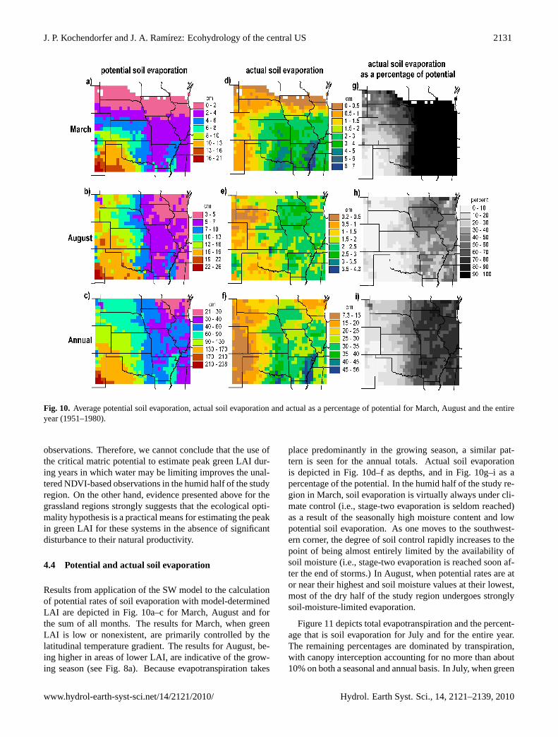
Fig. 10. Average potential soil evaporation, actual soil evaporation and actual as a percentage of potential for March, August and the entireyear (1951–1980).

observations. Therefore, we cannot conclude that the use ofthe critical matric potential to estimate peak green LAI dur-ing years in which water may be limiting improves the unal-tered NDVI-based observations in the humid half of the studyregion. On the other hand, evidence presented above for thegrassland regions strongly suggests that the ecological opti-mality hypothesis is a practical means for estimating the peakin green LAI for these systems in the absence of significantdisturbance to their natural productivity.

4.4 Potential and actual soil evaporation

Results from application of the SW model to the calculationof potential rates of soil evaporation with model-determinedLAI are depicted in Fig. 10a–c for March, August and forthe sum of all months. The results for March, when greenLAI is low or nonexistent, are primarily controlled by thelatitudinal temperature gradient. The results for August, be-ing higher in areas of lower LAI, are indicative of the grow-ing season (see Fig. 8a). Because evapotranspiration takes

place predominantly in the growing season, a similar pat-tern is seen for the annual totals. Actual soil evaporationis depicted in Fig. 10d–f as depths, and in Fig. 10g–i as apercentage of the potential. In the humid half of the study re-gion in March, soil evaporation is virtually always under cli-mate control (i.e., stage-two evaporation is seldom reached)as a result of the seasonally high moisture content and lowpotential soil evaporation. As one moves to the southwest-ern corner, the degree of soil control rapidly increases to thepoint of being almost entirely limited by the availability ofsoil moisture (i.e., stage-two evaporation is reached soon af-ter the end of storms.) In August, when potential rates are ator near their highest and soil moisture values at their lowest,most of the dry half of the study region undergoes stronglysoil-moisture-limited evaporation.

Figure 11 depicts total evapotranspiration and the percent-age that is soil evaporation for July and for the entire year.The remaining percentages are dominated by transpiration,with canopy interception accounting for no more than about10% on both a seasonal and annual basis. In July, when green



Fig. 11. Average total evapotranspiration and soil evaporation as a percentage of total evapotranspiration for July and the entire year(1951–1980).

LAI is at or near its peak, soil evaporation falls in the rangeof 10% to 30% of total evapotranspiration for the majority ofthe cells, with the percentages being more variable in the dryhalf of the study region. On an annual basis, soil evaporationcomprises between 30% and 60% of total evapotranspirationfor nearly all the cells. The distribution of percentages showssurprisingly little correlation to vegetation class or climate.This suggests that the generally lower vegetation cover andlower soil-surface resistances in the dry half of the study re-gion are more-or-less completely offset by the drier soil.

In contrast to vegetation class and climate, the influencesof soil texture are clear in the percentages in Fig. 11. The dif-ferences in LAI resulting from the differences in soil texturebetween the Pierre Shale Plains and the Sand Hills manifestthemselves as, respectively, regionally higher and lower per-centages of soil evaporation. In the humid half of the studyregion, the highest percentages of soil evaporation (i.e., thosein excess of 60%) are associated with the high-clay soils ofthe lower Mississippi River valley and Northeast Texas (seeFig. 3). The proximate cause of the higher percentages inregions of high clay content is the greater potential soil evap-

oration (see Fig. 10b, c) that results from the regionally lowerLAI (see Fig. 8a). If we look at soil evaporation as a percent-age of potential soil evaporation (see Fig. 10g–i), we see thatthe percentages are slightly higher than the surrounding cellsin the high clay areas of the humid half, while slightly lowerin the Pierre Shale Plains. This suggests that the lower diffu-sivity of the high-clay soils has a greater offsetting effect tothe higher moisture content in the Pierre Shale Plains than inthe humid regions. The difference has mainly to do with thedegree to which soil evaporation is controlled by moisturecontent; in the humid half of the study region, at least 60%of the potential demand is met for nearly all the cells on anannual basis.

Although relatively new isotopic, sap-flow and eddy-covariance methods are increasingly being applied (e.g.,Smith and Allen, 1996), separate observation of soil evap-oration and transpiration has historically been difficult, andcontinues to be, particularly at the stand and larger scales,and over time periods representative of average climatic con-ditions. Therefore, there are not many data that can beused to validate the partitioning of evapotranspiration in the



Fig. 12. (a)Modeled average annual grassland transpiration (1951–

1980) for cells in which the natural vegetation is grassland or sa-vanna,(b) estimates of average annual TNPP (1989–1993) fromTieszen et al. (1997) as contained in the database of Zheng etal. (2003b), and(c) water use efficency calculated with (a) and (b).

model results. Nonetheless, a few studies were identifiedat sites in or near the study region. Of particular interestare the stable isotope study of Ferretti et al. (2003) and theenergy-balance measurement and modeling study of Mass-man (1992) conducted at the CPER. Those studies were re-viewed by Kochendorfer and Ramirez (2010) and found tobe in good agreement with model results for the CPER. TheirSDEM-SW results show that, over the growing season, soilevaporation is the dominant component of evapotransirationin April and May and a neglible component in August andSeptember, with the June and July percentages approximat-ing the average over the whole growing season. Even in thesparse canopy of the shortgrass steppe – measured peak LAIat the CPER ranges from 0.4–0.6 (Hazlett, 1992; Knight,1973), growing-season soil evaporation appears to averageone third or less of total evapotranspiration. Measurement-based studies from more arid environments in the southwestUSA (Dugas et al., 1996; Stannard and Weltz, 2006) indicatethat transpiration dominates there as well.

In comparison, to natural vegetation, more evapotranspi-ration partitioning studies have been conducted of crops,with a tendency to focus on irrigated systems. The cumu-lative impression from several such studies (Ashktorab etal., 1994; Klocke, 2003; Leuning et al., 1994; Massmanand Ham, 1994; Peters and Russell, 1959; Villabalobos andFereres, 1990), as well as from a review paper (Burt et al.,2005), is that cumulative growing-season soil evaporationranges from 20% to 50% of total evapotranspiration for well-watered crops – both irrigated and rain-fed. Thus crop per-centages in the literature are similar to those for semi-aridgrasslands and also in good agreement with the model re-sults in Fig. 10 (which were produced under the assumptionof rain-fed crops.) Variations in the literature values appearto be more dependent on irrigation and tilling schemes thanon climate or crop type.

Finally, we consider the empirical data on evapotranspi-ration partitioning in forests in the humid half of the studyregion. Eddy covariance measurements in deciduous forestsjust east of our study region (Grimmond et al., 2000; Wil-son et al., 2001) show evaporation from the forest floor to beabout 10% of total evapotranspiration at peak LAI. Becausemodel results in Fig. 13 show a contribution in July fromsoil evaporation of 10–30%, we can conclude that the modeltends to overestimate soil evaporation in humid forests. Thismay be the result of the upper bound on LAI being limited tosix. Another possible source of model error is the values ofsurface soil resistance for forests in Table 1 underestimatingthe mulching effect of the litter layer. In general, greater con-sideration needs to be given to the limitations of applying thetwo-component SW model (which was originally developedfor sparse crop canopies) to the taller and generally hetero-geneous, multi-leveled canopies of forests, woodlands andsavannas.



Fig. 13. Root-zone estimates of(a) residual moisture content,(b) pore size distribution index,(c) bubbling pressure, and(d) saturated

hydraulic conductivity.

5 Summary and conclusions

The SDEM as coupled to the SW canopy model has beenapplied to the central United States over a half-degree gridusing vegetation, soil and climate data from the Vegeta-tion/Ecosystem Modeling and Analysis Project (VEMAP),among other sources. A very good match of modeled meanannual runoff to contours of streamflow was achieved withonly minimal calibration of two evapotranspiration param-eters, indicating that mean annual evapotranspiration is ap-proximated well by the coupled models.

The interannual variation in peak green LAI is modeledthrough application of the hypothesis that, in any year inwhich water is significantly limiting, vegetation will drawsoil moisture down in the latter half of the growing seasonapproximately to the point at which the vegetation just beginsto experience water stress. The hypothesis is applied to max-imize the annual peak in green LAI, within upper and lowerbounds, by scaling the seasonal LAI curve by a single fac-

tor. Grid-cell specific curves were determined from NDVI-based estimates of green LAI. For the water-limited grass-land region, comparison of the means of model-determinedpeak green LAI and those of the unaltered NDVI-based ob-servations with ground-based observations of LAI and witha gridded datasets of above-ground net primary productionindicated that the model-determined values are at least as ac-curate as the unaltered observations. The lack of positivecorrelation between accumulated precipitation and the peakin observed green LAI for vegetation in the humid half ofthe study region suggest that the optimization hypothesis isof limited use in this region. However, the somewhat arbi-trary upper bound of six in both observed and modeled greenLAI may be masking greater spatial and interannual variabil-ity and, consequently, the role of water in determining thelong-term mean peak, particularly in the forested areas.

The partitioning of evapotranspiration in model resultsshowed little dependence on climate and vegetation type,with most of the variation across the study region attributable



July

mean time between storms mean storm depth

January

Fig. 14. Estimates of two of the statistics of the Poisson rectangular-pulse stochastic precipitation model for January and July.

to soil texture and the resultant differences in vegetation den-sity. The implication is that the higher (lower) soil mois-ture content in wetter (drier) climates is more-or-less offsetby the greater (lesser) amount of energy available at the soilsurface. At the low end, with approximately 25–35% of an-nual average evapotranspiration being soil evaporation, aremostly soils with high sand content. At the high end, with60–70% as soil evaporation, are soils with high clay con-tent. The results for grasslands and crops are well supportedby empirical observations in the literature. However, eddy-covariance studies from two deciduous forests near the studyregion suggest that the model overestimates soil evaporationin humid forests by a factor of as much as two. This callsinto question both the upper bound of six for the LAI andthe accuracy of the Shuttleworth-Wallace model (as coupledto the SDEM) for the heterogeneous, multi-level canopies offorests, woodlands and savannas. In general, our results andtheir validation help to clarify the wide-ranging results in thepartitioning of evapotranspiration that have been producedby other SVATS.

Appendix A

Parameter estimation

A1 Soil hydraulic parameters

The soil hydraulic parameters in the SDEM are those ofBrooks and Corey (1966), who formulate the dependency ofthe soil matric potential on soil moisture content as

9(s) = 9ss−1/m (A1)

where9(s) is the soil matric potential at a relative soil satu-ration ofs, 9s is the bubbling matric potential (i.e., the valueat which air entry begins), andm is the pore size distributionindex.s is defined by

s =θt −θr

nt −θr(A2)

whereθt is the total volumetric soil water content,θr is theresidual volumetric soil water content, andnt total porosity.Brooks and Corey formulate the dependency of the unsatu-rated hydraulic conductivity ons as

K(s) = Kssc (A3)



wherec is the pore disconnectedness index, which the au-thors show to be related to the pore size distribution indexby

c =2+3m

m(A4)

Grid-cell mean bulk density and percentages of sand, silt andclay from the VEMAP database were used to estimate valuesof the Brooks-Corey soil hydraulic parameters. Those dataare given for two soil layers: 0–50 cm and 50–150 cm, wherethe data for the former are used for root zone and the data forthe latter are used for the recharge zone, regardless of the ac-tual values used for the depth of the soil layers. Bulk densitywas converted to total porosity with the standard assumptionof a mineral density of 2.65 g/cm3. In order to capture thesignigicant variability of hydraulic properties within texturalclasses due differences in grain-size distribution, Kochendor-fer (2005) modeled the dependence ofθr, 9s andm on sandand clay percentages by multivariate linear regression. Thevalues of texture-specific hydraulic parameters reported byRawls et al. (1982) were assigned to the midpoint values ofsand and clay percentages for the corresponding texture classon the USDA triangle. The results of application of the re-gression equations to the VEMAP sand and clay percentagesfor the 0–50 cm layer are presented in Fig. 13a–c. FollowingRawls et al. (1982), Kochendorfer (2005) related the Brooks-Corey parameters toKs using an equation derived by Brut-saert (1967) based on a permeability model developed byChilds and Collis-George (1950). The equation was scaledto fit the textural-class geometric means reported by Cosbyet al. (1984) and Rawls et al. (1982). Shown in Fig. 13d arethe results for the root zone after a lower limit of 5.0 cm/dwas placed onKs.

A2 Storm statistics

Kochendorfer (2005) derived monthly values for the statisticsof the PRP precipitation model from hourly observations ofprecipitation as compiled by the National Climatic Data Cen-ter (NCDC) and made available on CD-ROM by EarthInfo,Inc. (EarthInfo, 1999). Those observations were taken byrecording rain gauges located at National Weather Service,Federal Aviation Administration, and Cooperative Observerstations. Thousands of these stations began making observa-tions in and soon after 1948 and continue through the present.The 50-year period from 1949 to 1998 was selected for es-timation of the parameter values of the precipitation model.Stations in the NCDC database were included in the anal-ysis if they have records for at least 40 of the 50 years andhave no more than 20% missing data for the available years.Within an area extending 2.5◦ latitude and longitude beyondthe boundaries of the study region, 706 stations met those cri-teria. Ordinary kriging (detailed descriptions of which can befound elsewhere; e.g., Kitanidis, 1993) was selected a priorias the preferred method for interpolating the station statisticsto the half-degree grid of the study region. The results for

January and July are presented in Fig. 14 for two of the moreimportant statistics:mtb, the mean time between storms, andmh, the mean depth of storms. The former primarily con-trols the frequency with which stage-two soil evaporation isreached, while the latter primarily controls the partitioningbetween infiltration and surface runoff.

In an equilibrium calculation of the monthly water bal-ance, the PRP statistics are all that are needed (see Kochen-dorfer and Ramirez, 2010). In Eagleson’s application of hisoriginal model to estimating the interannual variability ofrunoff, he perturbs the model with variations in annual pre-cipitation as sampled from its PDF (as predicted by the PRPmodel), while leaving the values of the PRP statistics alone(Eagleson, 1978g). However, a given value of precipitationover some period that is larger (smaller) than long-term meanincreases the likelihood of greater (fewer) number of stormsfor that time period, as well the likelihood for deeper (shal-lower) storms than the mean depth. By applying Bayes’ The-orem to the PRP model, Salvucci and Song (2000) deriveprobability distributions for the number of storms and themean storm depth over a given period conditioned on the ac-tual precipitation for that period. We use their methodologyto condition the monthly mean values of the PRP statisticsin each month on the observed VEMAP/PRISM total for thegiven month and grid cell. Details can be found in Kochen-dorfer (2005).

A3 Monthly climate variables

In addition to being the source of monthly precipitation, theVEMAP database provided monthly mean temperatures, aswell as two other variables necessary for implementation ofthe SW model: incoming solar radiation and water vaporpressure. Four variables necessary for implementation of theSW model not included in the VEMAP database are net long-wave radiation, surface albedo, air pressure and monthlywindspeed (the last being provided only as a seasonal clima-tology). Net long-wave radiation was estimated from cloudi-ness, surface temperature and humidity using a methodol-ogy outlined by Sellers (1965). Cloudiness was estimatedas a linear function of the ratio of solar radiation incidentat the surface to that incident at the top of the atmosphere,with the slope and intercept visually calibrated to maps of aclimatology of observed percent sunshine (Baldwin, 1973).Due to a lack of remotely sensed surface albedo over the en-tire modeling period, a gridded, monthly climatology createdby Hobbins et al. (2001) based on Gutman (1988) was used.Surface air pressure and surface windspeed were interpolatedfrom monthly values produced by the NOAA-CIRES Cen-ter for the Diagnosis of Climate (http://www.cdc.noaa.gov/cdc/reanalysis/) from results of the NCEP/NCAR reanalysisproject (Kalnay et al., 1996). The remaining, water-vapor-related variables were calculated from vapor pressure, airtemperature and air pressure using standard formulas pre-sented by Shuttleworth (1993).


http://www.cdc.noaa.gov/cdc/reanalysis/

http://www.cdc.noaa.gov/cdc/reanalysis/


Acknowledgements.This work was partially supported by theNational Institute for Global Environmental Change through theUS Department of Energy (Cooperative Agreement DE-FC03-90ER61010). Some of this work was performed while the secondauthor was on sabbatical leave at the Swiss Federal Institute ofTechnology (ETH-Z) whose support is gratefully acknowledged.We sincerely acknowledge the review comments of the editor andtwo anonymous reviewers.

Edited by: S. Manfreda

References

Ashktorab, H., Pruitt, W. O., and Paw, K. T.: Partitioning of evap-otranspiration using lysimeter and micro-Bowen-ratio system, J.Irrig. Drai. E.-ASCE, 120(2), 450–464, 1994.

Baldwin, J. L.: Climates of the United States, US Department ofCommerce, National Oceanic and Atmospheric Administration,Washington, DC, 113 pp., 1973.

Bond, J. J. and Willis, W. O.: Soil water evaporation: surfaceresidue rate and placement effects, Soil Sci. Soc. Am. Pro., 33,445–448, 1969.

Boyer, J. S.: Resistances to water transport in soybean, bean, andsunflower, Crop Sciences, 11, 403–407, 1971.

Brooks, R. H. and Corey, A. T.: Properties of porous media af-fecting fluid flow, J. Irrigation Drainage Division of AmericanSociety of Civil Engineers, IR2, 61–88, 1966.

Brutsaert, W.: Some methods of calculating unsaturated permeabil-ity, T. ASAE, 400–404, 1967.

Buermann, W., Wang, Y., Dong, J., Zhou, L., Zeng, X., Dickinson,R. E., Potter, C. S., and Myneni, R. B.: Analysis of a multi-year global vegetation leaf area index data set, J. Geophys. Res.,107(D22), 4646–4664, 2002.

Burt, C. M., Mutziger, A. J., Allen, R. G., and Howell, T. A.: Evap-oration research: Review and interpretation, J. Irrig. Drain. E.-ASCE, 131(1), 37–58, 2005.

Camillo, P. J. and Gurney, R. J.: A resistance parameter for bare-soilevaporation models, Soil Sci., 141(2), 95–105, 1986.

Childs, E. C. and Collis-George, N.: The permeability of porousmaterials, Proc. Roy. Soc. A, A201, 392–405, 1950.

Choudhury, B. J., DiGirolamo, N. E., Susskind, J., Darnell, W. L.,Gupta, S. K., and Asrar, G.: A biophysical process-based esti-mate of global land surface evaporation using satellite and an-cillary data – II. Regional and global patterns of seasonal andannual variations, J. Hydrol., 205(3–4), 186–204, 1998.

Choudhury, B. J. and Monteith, J. L.: A four-layer model for theheat budget of homogeneous land surfaces, Q. J. Roy. Meteor.Soc., 114, 373–398, 1988.

Cosby, B. J., Hornberger, G. M., Clapp, R. B., and Ginn, T. R.: Astatistical exploration of the relationships of soil moisture char-acteristics to the physical properties of soils, Water Resour. Res.,20(6), 682–690, 1984.

Cowan, I. R.: Transport of water in the soil-plant-atmosphere sys-tem, J. Appl. Ecol., 2, 221–239, 1965.

Cowan, I. R. and Milthorpe, F. L.: Plant factors influencing the wa-ter status of plant tissues, in: Water Deficits and Plant Growth,Vol. 1: Development, Growth and Measurement, edited by: Ko-zlowski, T. T., Academic Press, New York, 137–193, 1968.

Daly, C., Neilson, R. P., and Phillips, D. L.: A statistical-topographic model for mapping climatological precipitation, J.Appl. Meteorol., 33, 140–158, 1994.

Denmead, O. T.: Temperate cereals, in: Vegetation and the Atmo-sphere, edited by: Monteith, J. L., Academic Press, New York,1–31, 1976.

Denmead, O. T. and Shaw, R. H.: Availability of soil water to plantsas affected by soil moisture content and meteorological condi-tions, Agron. J., 54, 385–390, 1962.

Dickinson, R. E., Henderson-Sellers, A., and Kennedy, P. J.:Biosphere-Atmosphere Transfer Scheme (BATS) Version 1e asCoupled to the NCAR Community Climate Model, NCAR Tech-nical Note, National Center for Atmospheric Research, Boulder,CO, 1993.

Dugas, W. A., Hicks, R. A., and Gibbens, R. P.: Structure and func-tion of C-3 and C-4 Chihuahuan Desert plant communities, En-ergy balance components, J. Arid Environ., 34(1), 63–79, 1996.

Eagleson, P. S.: Climate, soil, and vegetation: 1. Introduction towater balance dynamics, Water Resour. Res., 14(5), 705–712,1978a.

Eagleson, P. S.: Climate, soil, and vegetation: 2. The distributionof annual precipitation derived from observed sequences, WaterResour. Res., 14(5), 713–721, 1978b.

Eagleson, P. S.: Climate, soil, and vegetation: 3. A simplified modelof soil moisture movement in the liquid phase, Water Resour.Res., 14(5), 722–730, 1978c.

Eagleson, P. S.: Climate, soil, and vegetation: 4. The expected valueof annual evapotranspiration, Water Resour. Res., 14(5), 731–739, 1978d.

Eagleson, P. S.: Climate, soil, and vegetation: 5. A derived distribu-tion of storm surface runoff, Water Resour. Res., 14(5), 740–748,1978e.

Eagleson, P. S.: Climate, soil, and vegetation: 6. Dynamics ofthe annual water balance, Water Resour. Res., 14(5), 749–764,1978f.

Eagleson, P. S.: Climate, soil, and vegetation: 7. A derived distribu-tion of annual water yield, Water Resour. Res., 14(5), 765–776,1978g.

EarthInfo: CDROM of National Climate Data Center Hourly Pre-cipitation Records, EarthInfo, Boulder, CO, 1999.

Epstein, H. E., Lauenroth, W. K., Burke, I. C., and Coffin, D. P.:Productivity patterns of C3 and C4 functional types in the USgreat plains, Ecology, 78(2), 722–731, 1997a.

Federer, C. A.: A soil-plant-atmosphere model for transpiration andavailability of soil water, Water Resour. Res., 15(2), 555–562,1979.

Ferretti, D. F., Pendall, E., Morgan, J. A., Nelson, J. A., LeCain, D.,and Mosier, A. R.: Partitioning evapotranspiration fluxes froma Colorado grassland using stable isotopes: Seasonal variationsand ecosystem implications of elevated atmospheric CO2, PlantSoil, 254(2), 291–303, 2003.

Gardner, W. R.: Dynamic aspects of water availability to plants,Soil Sci., 89(2), 63–73, 1960.

Gardner, W. R. and Ehlig, C. F.: The influence of soil water on tran-spiration by plants, J. Geophys. Res., 68(20), 5719–5725, 1963.

Gebert, W. A., Graczyk, D. J., and Krug, W. R.: Average annualrunoff in the United States, 1951–80, Online available at:http://water.usgs.gov/pubs/. US Geological Survey, 1987.

Geraghty, J. J. and Miller, D. W.: Water Atlas of the United States,


http://water.usgs.gov/pubs/

http://water.usgs.gov/pubs/


Water Information Center, Port Washington, 122 pp., 1973.Gollan, T., Passioura, J. B., and Munnus, R.: Soil water status af-

fects the stomatal conductance of fully turgid wheat and sun-flower leaves, Aust. J. Plant Physiol., 13, 459–464, 1986.

Grimmond, C. S. B., Hanson, P. J., Cropley, F., Schmid, H. P., andWullschleger, S.: Evapotranspiration rates at the Morgan MonroeState Forest Ameriflux site: a comparison of results from eddycovariance turbulent flux measurements and sap flow techniques,Proceedings of 15th AMS Symposium on Hydrology, AmericanMeteorological Society, Long Beach, CA, 158–161, 2000.

Guswa, A. J., Celia, M. A., and Rodriguez-Iturbe, I.: Models of soilmoisture dynamics in ecohydrology: a comparative study, WaterResour. Res., 38(9), 1166–1181, 2002.

Gutman, G.: A simple method for estimating monthly mean albedofrom AVHRR data, J. Appl. Meteorol., 27, 973–988, 1988.

Havranek, W. M. and Benecke, U.: Influence of soil moistureon water potential, transpiration and photosynthesis of coniferseedlings, Plant. Soil., 49, 91–103, 1978.

Hazlett, D.: Leaf area development of four plant communities in theColorado steppe, Am. Midl. Nat., 127, 276–289, 1992.

Hellkvist, J., Richards, G. P., and Jarvis, P. G.: Vertical gradientsof water potential and tissue water relations in sitka spruce treesmeasured with the pressure chamber, J. Appl. Ecol., 11, 637–667, 1973.

Hobbins, M. T., Ramırez, J. A., Brown, T. C., and Claessens, L. H.J. M.: The complementary relationship in estimation of regionalevapotranspiration: The complementary relationship areal evap-otranspiration and advection-aridity models, Water Resour. Res.,37(5), 1367–1387, 2001.

Hollinger, S. E. and Isard, S. A.: A soil moisture climatology ofIllinois, J. Climate, 7, 822–833, 1994.

Jackson, R. B., Canadell, J., Ehleringer, J. R., Mooney, H. A., Sala,O. E., and Schulze, E. D: A global analysis of root distributionsfor terrestrial biomes, Oecologia, 108, 389–411, 1996.

Jackson, R. B., Schenk, H. J., Jobbagy, E. G., Canadell, J., Colello,R. E., Dickinson, R. E., Field, C. B., Friedlingstein, P., Heimann,M., Hibbard, K., Kicklighter, D. W., Kleidon, A., Neilson, R. P.,Parton, W. J., Sala, O. E., and Sykes, M. T.: Belowground con-sequences of vegetation change and their treatment in models,Ecol. Appl., 10(2), 470–483, 2000.

Jarvis, P. G., James, G. B., and Landsberg, J. J.: Conifer forest,in: Vegetation and the Atmosphere, edited by: Monteith, J. L.,Academic Press, New York, 171–236, 1976.

Kalnay, E., Kanamitsu, M., Kistler, R., Collins, W., Deaven, D.,Gandin, L., Iredell, M., Saha, S., White, G., Woollen, J., Zhu, Y.,Chelliah, M., Ebisuzaki, W., Higgins, W., Janowiak, J., Mom K.C., Ropelewski, C., Wang, J., Leetmaa, A., Reynolds, R., Jenne,R., and Joseph, D.: The NCEP/NCAR 40-year reanalysis project,B. Am. Meteorol. Soc., 77(2), 437–471, 1996.

Kitanidis, P. K.: Geostatistics, in: Handbook of Hydrology, editedby: Maidment, D. R., McGraw-Hill, New York, 20.1–20.39,1993.

Kittel, T. G. F., Rosenbloom, N. A., Painter, T. H., Schimel, D.S., and Participants, V. M.: The VEMAP integrated database formodeling United States ecosystem/vegetation sensitivity to cli-mate change, J. Biogeogr., 22(4–5), 857–862, 1995.

Klocke, N. L.: Water savings from crop residue in irrigated corn,Central Plains Irrigation Conference Proceedings, Colby, KS,134–142, 2003.

Knight, D.: Leaf area dynamics of a shortgrass prairie in Colorado,Ecology, 54(3), 891–896, 1973.

Kochendorfer, J. P.: A monthly, two-soil-layer statitistical-dynamical water balance model for ecohydrologically focusedclimate impact assessment, Ph.D. dissertation, Department ofCivil Engineering, Colorado State University, Fort Collins, CO,211 pp., 2005.

Kochendorfer, J. P. and Ramırez, J. A.: Modeling the monthlymean soil-water balance with a statistical-dynamical ecohydrol-ogy model as coupled to a two-component canopy model, Hy-drol. Earth Syst. Sci., 14, 2099–2120, doi:10.5194/hess-14-2099-2010, 2010.

Korner, C., Scheel, J. A., and Bauer, H.: Maximum leaf diffusiveconductance in vascular plants, Photosynthetica, 13(1), 45–82,1979.

Kramer, P. J.: Water Relations of Plants. Academic Press, NewYork, 489 pp., 1983.

Lafleur, P. M. and Rouse, W. R.: Application of an energy combi-nation model for evaporation from sparse canopies, Agr. ForestMeteorol., 49, 135–153, 1990.

Larcher, W.: Physiological Plant Ecology, Springer-Verlag, NewYork, 297 pp., 1980.

Lawrence, D. M., Thornton, P. E., Oleson, K. W., and Bonan, G. B.:The Partitioning of Evapotranspiration into Transpiration, SoilEvaporation, and Canopy Evaporation in a GCM: impacts onLand – Atmosphere Interaction, J. Hydrometeorol., 8(3), 862–880, 2007.

Leuning, R., Condon, A. G., Dunin, F. X., Zegelin, S., and Den-mead, O. T.: Rainfall Interception and Evaporation from SoilBelow a Wheat Canopy, Agr. Forest Meteorol., 67(3–4), 221–238, 1994.

Los, S. O., Collatz, G. J., Sellers, P. J., Malstrom, C. M., Pollack, N.H., DeFries, R. S., Bounoua, L., Parris, M. T., Tucker, C. J., andDazlich, D. A.: A global 9-yr biophysical land surface datasetfrom NOAA AVHRR data, J. Hydrometeorol., 1, 183–199, 2000.

Luxmoore, R. J. and Sharma, M. L.: Runoff responses to soil het-erogeneity: Experimental and simulation comparisons for twocontrasting watersheds, Water Resour. Res., 16(3), 675–684,1980.

Mahfouf, J.-F., Ciret, C., Ducharne, A., Irannejad, P., Noilhan, J.,Shao, Y., Thornton, P., Xue, Y., and Yang, Z.-L.: Analysis oftranspiration results from the RICE and PILPS workshop, GlobalPlanet. Change, 13, 73–88, 1996.

Massman, W. J.: A Surface-Energy Balance Method for Partition-ing Evapotranspiration Data into Plant and Soil Components fora Surface with Partial Canopy Cover, Water Resour. Res., 28(6),1723–1732, 1992.

Massman, W. J. and Ham, J. M.: An Evaluation of a Surface-Energy Balance Method for Partitioning Et Data into Plant andSoil Components for a Surface with Partial Canopy Cover, Agr.Forest Meteorol., 67(3–4), 253–267, 1994.

Monteith, J. L.: Evaporation and the environment, Symposia of theSociety for Experimental Biology, 19, 205–234, 1965.

Neilson, R. P.: A model for predicting continental-scale vegetationdistribution and water balance, Ecol. Appl., 5(2), 362–385, 1995.

Nemani, R. R. and Running, S. W.: Satellite monitoring ofglobal land cover changes and their impact on climate, ClimaticChange, 31(2), 395–413, 1995.

Newman, B. D., Wilcox, B. P., Archer, S. R., Breshears, D. D.,



Dahm, C. N., Duffy, C. J., McDowell, N. G., Phillips, F. M.,Scanlon, B. R., and Vivoni, E. R.: Ecohydrology of water-limited environments: a scientific vision, Water Resour. Res., 42,W06302, doi:10.1029/2005WR004141, 2006.

Newman, E. I.: Resistance to water flow in soil and plant: I. Soilresistance in relation to amounts of root: theoretical estimates, J.Appl. Ecol., 6, 1–112, 1969.

Noy-Meir, I.: Desert ecosystems: Environment and producers, An-nual Review of Ecological Systems, 4, 25–51, 1973.

Penman, H. L.: Natural Evaporation from open water, bare soil andgrass, P. Roy. Soc. A., A193, 120–145, 1948.

Peters, D. B. and Russell, M. B.: Relative water losses by evap-oration and transpiration in field corn, Soil Sci. Soc. Am. Pro.,23(2), 170–173, 1959.

Phillip, J. R.: Theory of infiltration. Advances in Hydroscience, 5,215–296, 1969.

Prince, S., Haskett, J., Steininger, M., Strand, H., and Wright, R.:Net primary production of US midwest croplands from agricul-tural harvest yield data, Ecol. Appl., 11(3), 1194–1205, 2001.

Rauner, J. L.: Deciduous Forest, in: Vegetation and the Atmo-sphere, edited by: Monteith, J. L., Academic Press, New York,241–262, 1976.

Rawls, W. J., Brakensiek, D. L., and Saxton, K. E.: Estimation ofSoil Water Properties, T. ASAE, 1316–1320, 1982.

Richter, H.: The water status in the plant; experimental evidence,in: Water and Plant Life, edited by: Lange, O. L., Kappe, L.,and Schulze, E. D., Problems and Modern Approaches, Springer-Verlag, New York, 42–58, 1976.

Ripley, E. A. and Redmann, R. E.: Grassland, in: Vegetation andthe Atmosphere, Monteith, J. L., Academic Press, New York,351–396, 1976.

Ritchie, J. T., Rhoades, E. D., and Richardson, C.,W.: Calculatingevaporation from native grassland watersheds, T. ASAE, 19(6),1098–1103, 1976.

Robock, A., Vinnikov, K. Y., Srinivasan, G., Entin, J. K., Hollinger,S. E., Speranskaya, N. A., Liu, S., and Namkhai, A.: The globalsoil moisture data bank, B. Am. Meteorol. Soc., 81, 1281–1299,2000.

Rodriguez-Iturbe, I.: Ecohydrology: A hydrologic perspective ofclimate-soil-vegetation dynamics, Water Resour. Res., 36(1), 3–10, 2000.

Ross, J.: Radiative transfer in plant communities, in: Vegetation andthe Atmosphere, edited by: Monteith, J. L., Vol. 1: Principles,Academic Press, 13–55, 1975.

Running, S. W. and Hunt, E. R.: Generalization of a forest ecosys-tem process model for other biomes, BIOME-BGC, and an appli-cation for global-scale models, Scaling Physiological Processes:Leaf to Globe, Academic Press, Inc, 141–158, 1993.

Rutter, A. J.: The hydrological cycle in vegetation, in: Vegetationand the Atmosphere, edited by: Monteith, J. L., Vol. 1: Princi-ples, Academic Press, 111–154, 1975.

Sala, O. E., Lauenroth, W. K., Parton, W. J., and Trlica, M. J.: Waterstatus of soil and vegetation in a shortgrass steppe, Oecologia, 48,327–331, 1981.

Sala, O. E., Parton, W. J., Joyce, L. A., and Lauenroth, W. K.: Pri-mary production of the central grassland region of the UnitedStates, Ecology, 69(1), 40–45, 1988.

Salvucci, G. D. and Song, C.: Derived distributions of stormdepth and frequency conditioned on monthly total precipita-

tion: Adding value to historical and satellite-derived estimatesof monthly precipitation, J. Hydrometeorol., 1, 113–120, 2000.

Schenk, H. J. and Jackson, R. B.: The global biogeography of roots,Ecol. Monogr., 72(2), 311–3228, 2002.

Schulze, E. D., Kelliher, F. M., Korner, C., Lloyd, J., and Leun-ing, R.: Relationships among maximum stomatal conductance,ecosystem surface conductance, carbon assimilation rate, andplant nitrogen nutrition: a global ecology scaling exercise, Annu.Rev. Ecol. Syst., 25, 629–660, 1994.

Scurlock, J. M. O., Asner, G. P., and Gower, S. T.: Global leaf areaindex data from field measurements, Oak Ridge National Labo-ratory Distributed Active Archive Center, 1938–2000, 2001.

Sellers, P. J., Heiser, M. D., and Hall, F. G.: Relation between sur-face conductance and spectral vegetation indices at intermediate(100 m2 to 15 km2) length scales, J. Geophys. Res., 97(D17),19033–19059, 1992.

Sellers, P. J., Randall, G. J., Collatz, G. J., Berry, J. A., Field, C.B., Dazlich, D. A., Zhang, C., Collelo, G. D., and Bounoua, L.:A revised land surface parameterization (SiB2) for atmosphericGCMs, Part I: Model formulation, J. Climate, 9, 676–705, 1996.

Sellers, W. D.: Physical Climatology, The University of ChicagoPress, Chicago, 272 pp., 1965.

Shuttleworth, W. J.: Evaporation, in: Handbook of Hydrology,edited by: Maidment, D. R., McGraw-Hill, New York, 4.1–4.53,1993.

Shuttleworth, W. J. and Wallace, J. S.: Evaporation from sparsecrops: an energy combination theory, Q. J. Roy. Meteor. Soc.,111, 839–855, 1985.

Smith, D. M. and Allen, S. J.: Measurement of sap flow in plantstems, J. Exp. Bot., 47, 1833–1844, 1996.

Stannard, D. I. and Weltz, M. A.: Partitioning evapotranspirationin sparsely vegetated rangeland using a portable chamber, Wa-ter Resour. Res., 42(2), W02413, doi:10.1029/2005WR004251,2006.

Thornthwaite, C. W.: An approach toward a rational classificationof climate, Geogr. Rev., 38, 55–94, 1948.

Tieszen, L. L., Reed, B. C., Bliss, N. B., Wylie, B. K., and De-Jong, D. D.: NDVI, C3 and C4 production, and distributions ingreat plains grassland land cover classes, Ecol. Appl., 7(1), 59–78, 1997.

USGS: Map of Seasonal Land Cover Regions, US Geological Sur-vey, US Department of Interior, Washington DC, 1993.

van den Honert, T. H.: Water transport in plants as a catenary pro-cess, Discuss. Faraday Soc., 3, 146–153, 1948.

Villabalobos, F. J. and Fereres, E.: Evaporation measurements be-neath corn, cotton, and sunflower canopies, Agron. J., 82, 1153–1159, 1990.

Wilson, K. B., Hanson, P. J., Mulholland, P. J., Baldocchi, D. D.,and Wullschleger, S. D.: A comparison of methods for deter-mining forest evapotranspiration and its components: sap-flow,soil water budget, eddy covariance and catchment water balance,Agr. Forest Meteorol., 106(2), 153–168, 2001.

Woodward, F. I.: Climate and Plant Distribution, Cambridge Uni-versity Press, Cambridge, 174 pp., 1987.

Zheng, D., Prince, S., and Wright, R.: Terrestrial net primary pro-duction estimates for 0.5◦ grid cells from field observations: acontribution to global biogeochemical modeling, Global ChangeBiol., 9, 46–64, 2003.


ecohydrologic controls on vegetation density and

Documents