ECO 200: Advanced Principles of Economics: Concepts and Applications

Syllabus for Part II: Auctions

LECTURES

Lecture will take place on Mondays and Wednesdays from11:00am-12:20 pm. INSTRUCTOR

Professor Kenneth Hendricks Email: kenhen@princeton.edu Office: 211 Fisher Hall Phone (609) 258-XXXX Office hours: 11:00-12:00 AM, Tuesday and Thursday or by appointment

PRECEPTOR

Luke B. Willard Email: lwillard@Princeton.EDU Office: Wallace Hall Office hours: By appointment

GRADES AND COURSE REQUIREMENTS

Your grade for Part II will be based upon problem sets and an exam. COURSE OUTLINE October 11 & 13: Auctions as a Game of Strategy

• Overview • Formalizing a game of strategy • Solving games of strategy

Readings: *Chapters 1, 2, 3, and 4 of Games of Strategy by Avinash Dixit and Susan Skeath. Klemperer, P.D., (1999) “Auction Theory: A Guide to the Literature”, Journal of

Economic Surveys. McAfee, R.P. and J. McMillan (1987), “Auctions and Bidding”, Journal of Economic

Literature. Klemperer, P.D. (2004) “Why Every Economist Should Learn Some Auction Theory”, Advances in Economics and Econometrics: Theory and Applications.

October 18 and 20: Standard Auctions with Private Values

• Experiments • Equilibrium Bidding • Efficiency and Revenues

Readings: *Riley, J.G. (1989) “Expected Revenue from Open and Sealed Bid Auctions”, Journal of

Economic Perspectives. *Milgrom, P. (1989) “Auctions and Bidding: A Primer”, Journal of Economic of

Perspectives. Riley, J.G. and W. Samuelson (1981), “Optimal Auctions”, American Economic Review. Bulow, J. and D.J. Roberts (1989), “The Simple Economics of Optimal Auctions”,

Journal of Political Economy. November 1: Winner’s Curse

• Experiment • Application to Auctions of OCS Drainage Leases

Readings: *Hendricks, K. and R.H. Porter (1988), “An Empirical Study of an Auction with

Asymmetric Information”, American Economic Review. Klemperer, P.D. (1998), “Auctions with Almost Common Values”, European Economic

Review. Bulow, J.I. and P. Klemperer (2002), “Prices and the Winner’s Curse”, Rand Journal. November 3: All-Pay Auction

• Experiment • Application to BSB versus Sky Television

Readings: *Harvard Business School Case Study: British Satellite Broadcasting Versus Sky

Television. Hendricks, K. and R.H. Porter (1996), “The Timing and Incidence of Exploratory

Drilling on Offshore Wildcat Tracts, American Economic Review.

November 8: Issues in Auction Design I: Spectrum Auctions

• Spectrum Auctions in U.S. • Spectrum Auctions in Britain • Spectrum Auctions in Europe

Readings:

Klemperer, P.D., “What Really Matters in Auction Design”, Journal of Economic Perspectives.

*McAfee, R.P. and McMillan, J. (1994) “Selling Spectrum Rights”, Journal of Economic Perspectives. *McAfee, R.P. and McMillan, J. (1996) “Analyzing the Airwaves Auction”, Journal of Economic Perspectives. *Binmore, K. and Klemperer, P. (2002) “The Biggest Auction Ever: The Sale of the

British 3G Telecom Licenses”, Economic Journal. *Klemperer, P. (2002) “How (Not) to Run Auctions: the European 3G Telecom Auctions”, European Economic Review. Klemperer, P. (2004) “Using and Abusing Economic Theory – Lessons from Auction

Design”.

November 10: Issues in Auction Design II: Internet Auctions • eBay: hard close and Buy-it-Now options • Google IPO

Readings: Lucking-Reiley, D. (2000) “Auction on the Internet: What’s being Auctioned and How?”,

Journal of Industrial Economics. *Roth, A. and A. Ockenfels (2002), “Last Minute Bidding and the Rules for Ending

Second-Price Auctions: Evidence from eBay and Amazon Auctions on the Internet”, American Economic Review.

*Klemperer, P.D., editorials in Financial Times, May 3, 2004 and in Economist, May 8, 2004

I. Introduction to Auctions

A. OVERVIEW In the theory of competitive markets, buyers decide how much to buy and sellers decide how much to supply taking the market price as fixed, and the market price is determined by the assumption of market clearing: it equates supply to demand. The theory is silent about the process by which buyers and sellers determine the price that clears the market. The standard story is that the market acts like an auctioneer: buyers submit their willingness to pay schedules and sellers submit their marginal cost schedules and the auctioneer finds the price at which the amount that buyers are willing to buy is equal to the amount that sellers are willing to supply. This story assumes that buyers and sellers will tell the truth. The justification of this assumption is that each trader’s transactions are negligible compared to the total volume of trade in the market. The main conclusion of the theory is that the competitive market is an efficient allocation mechanism: at the market-clearing price, the marginal buyer’s willingness to pay is just equal to the marginal cost of supply. Hence, all gains from trade are exhausted. Auctions are frequently used to determine trades and terms of trade in multilateral bargaining environments where buyer and/or sellers are not negligible. Examples include government sales of timber and mineral rights, SO2 emission permits, spectrum licenses, electricity, defense contracts, and treasury bills. In these examples, a single seller, the government, typically auctions a license to a small number of large corporations. The number of buyers in many electronic auction markets such as eBay is less than five. In these trading environments, auctions are a natural alternative to posting prices; they are an extension of the usual forms of bilateral bargaining (e.g., take-or-leave-it offers). The procedural rules specify precisely how market clearing determines prices. For example, oral auctions such as the English auction, find a clearing price by calling for bids in ascending order. In the oral Dutch auction, the clearing price is discovered by calling for bids in descending order. In an oral double auction, buyers and sellers are allow to cry out bids and offers that can be accepted immediately. Auctions, however, raises several basic issues about price determination that are ignored in the theory of competitive pricing: the role of private information, the consequences of strategic behavior, and the effect of more traders. Buyers know their willingness to pay, and sellers may know their willingness to sell, but this information is private. Unless they are given the right incentives, buyers are unlikely to tell the truth in fear that they will have to pay more for the item. The same is true of sellers, who want to obtain the highest possible price. The private information confers market power, and how this power is exercised is a major issue in the study of auctions. Auctions are not only a mechanism for price determination; they are also a mechanism for price discovery. Indeed, as we shall see, a major motivation for using auctions is to elicit revelation of preferences so that maximal gains from trade are realized.

The variety of possible procedural trading rules (i.e., kinds of auctions) is huge and we will study some of the more standard ones. For each type of auction, we focus on three questions: how will (should) buyers bid, how much does (should) the seller earn, and is the outcome efficient? Efficiency typically means that the item should go to the buyer who is willing to pay the most for it. The answers to these questions leads to another issue: optimizing the design of trading rules to either achieve more efficient allocations and/or more revenues. We will examine this issue in the context of spectrum auctions, eBay, and the recent Google IPO.

B. TYPES OF AUCTIONS Auctions, like many strategic situations, come in many forms. For example, consider a seller who has one item to allocate. Then one can roughly categorize common auction mechanisms into one of four cells:

Highest Bid Second Highest Bid Open Dutch English Closed First Price Sealed Bid

(FPSB) Second-price Sealed Bid (SPSB-Vickrey)

• Dutch auction: the auctioneer starts the bidding clock at a very high number and

lowers the bid level until someone says “stop”. The object is awarded to that bidder at the “stop” amount.

• English auction: the auctioneer starts the bidding clock at a very low number and raises the bid level (or bidders raise it) until all but one bidder drop out. The remaining bidder is awarded the object and pays the amount at which the second last bidder drops out.

• FPSB: each bidder submits her bid in a sealed envelope; bidder submitting the highest bid is awarded the object and pays her bid.

• SPSB: each bidder submits her bid in a sealed envelope; bidder submitting the highest bid is awarded the object and pays the second highest bid.

Another common auction that we will consider is known as the all-pay auction: the item goes to the bidder submitting the highest bid but every bidder pays her bid. C. AUCTIONS AND GAME THEORY 1. Auctions are games of conflict. In fact, they are typically winner-take-all contests. 2. Auctions are games in which the rules are fixed and well-defined. The seller chooses the rules and announces them. These rules determine who wins and how much each player is supposed to pay as a function of all of the bids submitted. Everyone knows the rules before they bid. In fact, one of the questions that we will consider is which rules should the seller choose.

3. Auctions are often games of imperfect information. Each bidder may know her own valuation of the item but is typically uncertain about the valuations of others. We will distinguish between situations of imperfect but symmetric information and situations of incomplete but asymmetric information. Examples: wildcat tracts – oil firms have different seismic information but quality of the information is similar; drainage tracts – oil firms that own the neighboring lease possesses superior drilling information. 4. The information that bidders have in making their bidding decisions in closed auctions is different than in open auctions. In closed auctions, each bidder submits his bid without knowing the bids of the other bidders. In open auctions, bidders can observe the bids of others and (potentially) react to them by raising the bid or by dropping out. We will refer to closed auctions as simultaneous move games and open auctions as sequential move games. Strategic thinking in simultaneous move games is fundamentally different than in sequential move games.

• Sequential: if I do this, the other player will do that, then I …. • Simultaneous: I think that he thinks that ….

Examples: Sequential: A bidder on eBay is trying to decide when and what to bid. If she bids higher than the existing high bid, her bid will not be observable to potential rivals but they will be aware that a higher bid has been submitted since the standing high bid will increase to the previous high bid. She worries that submitting a bid now, hours before the end of the auction, will trigger a competitive response from her rivals. On the other hand, if she lies low, waits until just before the end of the auction to submit a bid, she may be able to win the item and pay a lower price. This kind of reasoning gives rise to sniping. Simultaneous: ARCO is trying to determine how much it should bid in a FPSB for an oil and gas lease. Its bid depends upon how much it thinks that BP is going to bid. But the amount that BP bids depends in part upon what it thinks ARCO is going to bid. Therefore, in forecasting BP’s bids, ARCO needs to ask, how much does BP think we are going to bid? But BP is asking the same question: how much is ARCO going to bid? Therefore, ARCO also needs to ask: how much does BP think we think that BP is going to bid? 5. Auctions are non-cooperative games. Assuming joint bids are not permitted by the seller, each player must bid separately. 6. When bidders in an auction meet only in that auction, the auction is a one-shot game. However, in many cases, bidders bid against each other in more than one auction. For example, the FCC sold spectrum licenses for 52 Major Trading Areas simultaneously in

separate, ascending price auctions that ended only after no one wanted to raise the standing high bid on any of the licenses. Many states auction their highway repair contracts sequentially over the year and, as a result, construction firms find themselves bidding against each other repeatedly. Behavior in one-time games tends to be more unscrupulous, less cooperative. In games of repeated interaction, agents can use more sophisticated strategies. They can condition their actions in one auction on actions taken in other auctions. Examples: “tit-for-tat” bidding strategies. The availability of these kinds of strategies can lead to cooperative outcomes, even though the game is non-cooperative. Collusion in games of repeated interaction is a potentially important problem, and one that the seller must think about in choosing the rules of the auction.

Lecture 2

Private Value Auctions

The objectives of this lecture are as follows:

1. To participate in an English auction and a sealed-bid, second price auction when values are independent and private.

2. To characterize equilibrium bidding in these auctions and compare the predictions

from the theory against the data from the experiments.

3. To determine equilibrium expected revenues of these auctions and compare them against the outcomes from the experiments.

The Auction Environment

The objects that we will be auctioning are antique furniture: a chest of drawers, a dining room table, a bedstead, or a desk. For each item, there are n bidders. Each bidder’s valuation, V, is a random variable that can take any integer value between 0 and $99. Thus, the number of possible valuations is 100. The bidders’ values are independent draws from the set 0, 1,.…..,99. The probability of drawing any specific number is 1/100. That is, valuations are uniformly distributed – every number is equally likely. Each bidder knows his or her valuation but does not know the valuations of the other bidders. He or she believes that rival valuations are uniformly distributed as above. Each bidder’s valuation is private and represents his or her consumption value of the piece of furniture. (No resale.) In other words, even if a bidder would learn about the valuations of the other bidders, this information would not change his or her valuation of the piece of furniture.

The Sealed-Bid, Second-Price Auction Rules:

• Each bidder’s valuation: last two digits of the Social Security Number. • Each bidder submits a bid in a sealed envelop to me. • The bidder submitting the highest bid wins the piece of furniture and pays the

second highest bid submitted. • Ties are decided by the flip of a fair coin. • Losing bidders get zero.

Data: for each auction, we record the highest and second-highest bid, the winner’s valuation and profits, the highest and second highest valuations. These are as follows:

Group 1 Group 2 Group 3 Group 4 Highest Bid 99 88 99 80 Second Highest Bid 86 80 86 55 Winner’s Valuation 92 87 66 80 Winner’s Surplus 6 7 -20 25 Highest Value 92 90 90 80 Second Highest Value 86 87 86 55

Strategy: Any non-negative integer from 0 to 99. Equilibrium: What is the Nash equilibrium to this bidding game? Let V be your value, let B be your bid, and let Y be the highest bid by anybody else in the auction. Suppose B > V. Then, ignoring ties, there are three possibilities, depending upon Y.

1. Y > B > V: you lose, so your profits are zero. 2. B > Y > V: you win and your losses are V – Y < 0. 3. B > V > Y: you win and your profits are V – Y > 0.

In cases 1 and 3, lowering your bid from B to V has no affect on your payoffs. However, in case 2, lowering B to V eliminates losses. Hence, bidding more than your valuation is dominated by bidding V. Remark: Bidding V also dominates bidding V+1 because there is a chance that Y=V+1, in which case you win the object and pay V+1 with probability ½. Suppose V > B. Then, ignoring ties, once again there are three possibilities, depending upon Y.

1. Y < B < V: you win, and your profits are V – Y.

2. B < Y < V: you lose, and your profits are zero. 3. B < V < Y: you lose, and your profits are zero.

In cases 1 and 3, raising your bid from B to V yields no gain. But in case 2, raising your bid from B to V turns you into a winner and you gain V – Y > 0. Thus, bidding less than your valuation is dominated by bidding V. Remark: Bidding V also dominates V-1 since, if Y = V-1, you’re expected payoff from bidding V-1 is 1/2 and it is equal to 1 if you bid V. Results: 1. The game is dominance solvable. 2. The auction is efficient: buyer with highest valuation gets the item. 3. Everyone tells the truth so all valuations are revealed. This is a remarkable result. 4. If the Seller knew the valuations of the buyers, she could obtain full surplus by making a take-it-or-leave-it offer to the buyer with the highest valuation at a price equal to that buyer’s valuation. When valuations are private, the seller does not how much to offer and to whom she should make the offer. The private information gives the buyers some bargaining power. The best that the seller can do is to sell the item at a price equal to the second highest valuation. The difference between the highest and second highest valuation is the information rent that the buyer earns from the fact that valuations are private. In our experiment, the average (theoretical) price is (86 + 87 + 86 + 55)/4 = $78.2. The average value of the rent was (6 + 3 + 4 + 25)/4 = $9.20.

The English Auction Rules:

• Each bidder’s valuation: 100 minus the last two digits of the last four. • Auctioneer (Me) solicits an opening bid from somebody in the group. Anyone

who wants to drop out at this point announces that he/she is OUT. Exit is irreversible.

• The remaining bidders take turns raising the bid by $1 until there is only one bidder left.

• The last bidder gets the piece of furniture for a price equal to the bid at which the second last bidder drops out.

• Losing bidders get zero. Data: for each auction, we record the winning bid, the winner’s valuation and profits, the highest and second highest valuations.

Group 1 Group 2 Group 3 Group 4 Highest Bid 65 74 89 94 Winner’s Valuation 71 85 89 95 Winner’s Surplus 6 9 0 1 Highest Value 71 85 89 95 Second Highest Value 65 74 89 94

Average price is (65 + 74 + 89 + 94)/5 = $78 Average information rent = $4 Strategy: Specifies the bid level at which you drop out. Equilibrium: What is the Nash equilibrium to this bidding game?

• Bidding more than your willingness to pay is dominated by dropping out at your willingness to pay. If bidder i bids vi + 1 or more, and wins at that price, she loses money.

• Dropping out at a price that is lower than your willingness to pay is a mistake

since you could be leaving some money on the table.

Thus, dominance rules out all strategies except one:

• Stay in the bidding until B = vi -1.

• If it is your turn to bid at vi-1, then raise your bid by a dollar and, if your rival does not drop out at vi, drop out at vi + 1.

• If it is not your turn to bid at vi-1, then drop out at B = vi. The dominant strategy combination implies that the piece of furniture goes to the bidder with the highest valuation at a price that is either equal to the second-highest valuation or $1 above this value. It is the former if the bidder with the second-highest valuation has to bid at the second-highest valuation, and it is the latter if the bidder with the highest valuation has to bid at the second-highest valuation. Results: 1. The game is dominance solvable: optimal strategy does not depend upon bidding strategies of rivals and hence about your beliefs about their valuations or strategies. 2. The auction is efficient: bidder with highest valuation gets the item. 3. Valuations of losers are revealed. Highest valuation is not revealed. 4. Private information rent is the difference between highest and second highest valuation. 5. The English auction and the Second-Price, Sealed Bid auction yields identical outcomes (at least theoretically). Remark: The key assumption underlying the equivalence is that bidder valuations are private. That is, they do not change in the English auction as bidders learn their rivals’ valuations from when they exit the bidding.

PROBABILITY ARITHMETIC 1. Let pk denote the probability of drawing number k from the set Ω = 0,…,99. An event Q is a subset of Ω. Then, Probability of event Q = Σk∈Q pk. It is simply the sum of the probabilities of the numbers that lie in Q. Of course, in our case, pk = 1/100 for every number k. Examples:

• The probability that a bidder’s valuation is less than some number k is k/100. • The probability that a bidder’s valuation lies between 25 and 50 is 24/100.

2. The probability of drawing a number conditional on the event Q is the probability of drawing that number divided by the probability of the event Q. Probability of k|Q = pk/Σk∈Q pk. Example:

• The probability of drawing the number 30 conditional on the number lying between 25 and 50 is (1/100)/(24/100) = 1/24.

3. The expected value of a random variable V is given by the weighted average of all of its possible values using the probabilities as weights. E[V] = Σk pkk Example:

• The expected value of V when all numbers are equally likely splits the range: (99-0)/2 = 49.5. Intuition: there are 49 pairs of numbers that sum to 100; hence the weighted sum is equal to (1/100)(100)(49) + (50/100) = 49.5.

The expected value of a random variable V conditional on the event Q is given by the weighted average of all of possible values in Q divided by the probability of the event Q. E[V|Q] = [Σk∈Q (pkk)]/[ Σk∈Q pk]. Example:

• The expected value of a bidder’s valuation conditional on the event that the number is between 24 and 50 splits the range: 24 + (50-24)/2 = 37.

Lecture 4

1 The Sealed-Bid, First Price Auction

1.1 Rules:

• Each bidder’s valuation: first two digits of the last four.

• Each bidder submits a bid in a sealed envelop to me.

• The bidder submitting the highest bid wins the piece of furniture and pays the amountbid. Ties are settled by a coin toss.

• Losing bidders get zero.

1.2 Data:

For each auction, we record the highest and second-highest bid, the valuations of the highest

and second highest bidders, and if they are not the same, the highest and second highest

valuations.

1.3 Equilibrium:

What is the Nash equilibrium to this bidding game?

This bidding game is not dominance solvable. Each bidder will not want to bid her

value since doing so yields zero profits. She will want to shade her bid below her value;

the amount of shading depends upon the level of competition and the bidding behavior of

rivals. The benefit from a lower bid is a higher profit conditional on winning; the cost is a

lower probability of winning. The optimal shading factor balances these two effects.

From the perspective of each bidder, a rival’s bid is a random variable: it depends upon

the value that she draws and the bidding strategy that she pursues at each possible value.

Hence, in order to predict your rival’s bid, you need to know what she is going to bid at

every possible value, and not just at the value that she has drawn.

How do we conceptualize this situation? Harsanyi proposed the following approach. Let

Nature act first, giving each of the two bidders a value for the item. Then each player

chooses a bid, knowing their own value, but not that of the other bidder. A strategy in this

1

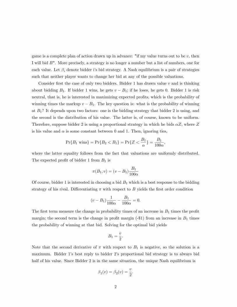
game is a complete plan of action drawn up in advance: "if my value turns out to be v, then

I will bid B". More precisely, a strategy is no longer a number but a list of numbers, one for

each value. Let βi denote bidder i’s bid strategy. A Nash equilibrium is a pair of strategies

such that neither player wants to change her bid at any of the possible valuations.

Consider first the case of only two bidders. Bidder 1 has drawn value v and is thinking

about bidding B1. If bidder 1 wins, he gets v − B1; if he loses, he gets 0. Bidder 1 is risk

neutral, that is, he is interested in maximizing expected profits, which is the probability of

winning times the markup v −B1. The key question is: what is the probability of winning

at B1? It depends upon two factors: one is the bidding strategy that bidder 2 is using, and

the second is the distribution of his value. The latter is, of course, known to be uniform.

Therefore, suppose bidder 2 is using a proportional strategy in which he bids αZ, where Z

is his value and α is some constant between 0 and 1. Then, ignoring ties,

PrB1 wins = PrB2 < B1 = PrZ <B1α = B1

100α,

where the latter equality follows from the fact that valuations are uniformly distributed.

The expected profit of bidder 1 from B1 is

π(B1, v) = (v −B1)B1100α

Of course, bidder 1 is interested in choosing a bid B1 which is a best response to the bidding

strategy of his rival. Differentiating π with respect to B yields the first order condition

(v −B1)1

100α− B1100α

= 0.

The first term measure the change in probability times of an increase in B1 times the profit

margin; the second term is the change in profit margin (-$1) from an increase in B1 times

the probability of winning at that bid. Solving for the optimal bid yields

B1 =v

2.

Note that the second derivative of π with respect to B1 is negative, so the solution is a

maximum. Bidder 1’s best reply to bidder 2’s proportional bid strategy is to always bid

half of his value. Since Bidder 2 is in the same situation, the unique Nash equilibrium is

β1(v) = β2(v) =v

2.

2

Consider next the case of n bidders. Once again assume that bidder 1’s rivals are

using proportional bid strategies and for simplicity we assume that they are using the same

strategy. In this case,

PrB1 wins = PrB1 > max(B2, .., BN ) = Prw2 < B1α...Prwn <

B1α

=

µB1100α

¶n−1.

Substituting this probability into bidder 1’s optimization problem and solving for his optimal

bid yields

B1 =(n− 1)v

n.

Thus, the unique Nash equilibrium is

β1(v) = ... = βn(v) =(n− 1)v

n.

1.4 Results

1. The auction is efficient: the bidder with the highest valuation wins the item.

2. The equilibrium is perfectly revealing of valuations. Although no one reports the

truth, bid functions are increasing. Hence, each bidder’s valuation can be obtained by

taking the inverse of the bid function: v = β−1(b). In the above example, solving for the

unknown value as a function of the bid gives

v =nb

n− 1 .

3. The information rent is positive and depends upon the difference between the valua-

tions of the highest and second-highest valuation. But it is not obvious that this difference

is equal to the difference in the two valuations.

2 The Dutch Auction

2.1 Rules:

• Each bidder’s valuation: 100 minus last two digits.

• I will count down from 100. The first buyer who says "Mine!" gets the item at the

number called.

3

• Losing bidders get zero.

2.2 Data:

For each auction, we record the winning bid, the valuation of the winning bidder, and the

highest and second highest valuations.

2.3 Equilibrium:

The strategic problem facing each bidder is the same as in the first-price sealed bid auction.

You never stop the bidding at a price above your value for then your profits are negative.

If no one has bid by the time that the price hits your valuation, you may choose to claim

the item but your profits are zero. By waiting and letting the price decline, you can earn

positive profits. The tradeoff at this point is the same as in the FPSB: by waiting, you

increase the profit from winning, but waiting also increases the risk of losing the item to a

rival bidder. These two effects are just balanced when the price reaches half of your value

(assuming n = 2), the same solution as in the FPSB auction. For this reason, the Dutch

auction is strategically equivalent to the FPSB auction.

Key assumption: independent, private values. You do not learn anything of relevance

as the price declines.

3 Revenues (Optional)

We have seen that the English and SPSB generate the same revenue. We have also shown

that bidding behavior in the Dutch auction is the same as in the FPSB auction. Hence,

revenues in these two auctions are also identical. But what about the revenues in the

second-price auctions compared to the first-price aucitons? The answer is not obvious.

Once again, to keep the calculatoins simple, lets assume that n = 2. With two bidders,

the winning bid in the second-price auctions is

WS = minV1, V2.

That is, it is the lower of the two valuations. More formally, WS is called the second order

statistic. The first order statistic is the maximum of the two values.

WF = maxV1, V2.

4

The winning bid in the first-price auctions (assuming bidders play the Nash equilibrium

strategies) is 12WF . That is, each bidder bids half of her value, and the winning bid is half

of the largest of the two values.

Claim 1 Expected revenues in all four auctions are identical.

The argument involves a little math and a little probability theory. To simplify the

arithmetic, I will assume that valuations can take any real number in the interval [0, 100].

Now lets think of WF as a random variable. The cumulative distribution of this random

variable, F1, is

F1(z) = PrWF < z = PrV1 < z, V2 < z = Pr(V1 < z) Pr(V2 < z)

=³ z

100

´³ z

100

´=

z2

10, 000

The probability density of WF is obtained by differentiating F1:

f1(z) = F 0(z) =2z

10000.

Then, the expected value of WF is

100Z0

z

µ2z

10000

¶dz =

¡1100

¢2 £23z3¤ |1000 = 2

3(100) = 66.67.

Recall that the winning bid is half of the expected value ofWF . Thus the expected revenues

to the seller from the first price auctions is 13(100) = $33.33

Now consider the revenues in the second-price auctions. Assume without loss of gener-

ality that V2 is larger than V1, that is, V2 is the first-order statistic. Then, given V2, the

expected value of V1 isV22, that is, it splits the interval from 0 to V2. But we know from

the above calculations that the expected value of the first order statistic is 23(100). Hence,

the expected value of the second-order statistic is 13(100).

Alternative derivation: the distribution of the second-order statistic is given by

F2(z) = 1− PrV1 > zPrV2 > z= 1− ¡1− z

100

¢2.

The density is

f2(z) =2100

¡1− z

100

¢.

5

Hence the expected value of WS is

1Z0

z 2100

¡1− z

100

¢dz = 1

100 [z2 − 2

31100z

3]|1000 = 13(100).

Q.E.D.

6

Lecture 4

The Winner’s Curse

The objectives of this lecture are as follows:

1. To participate in an English auction and a sealed-bid, first-price auction when values are common.

2. To characterize equilibrium bidding in a first-price auction in which one player

knows the value of the object and the other player does not.

3. Take the predictions of the theory to bid data from oil and gas drainage auctions. I. Introduction

The penny jar auctions are examples of auctions known as common value auctions. The value of the jar of pennies is the same for all bidders. Each of you looked at the jar and estimated the number of pennies in the jar. Some bidders guessed numbers that were too high, and some of you guessed numbers that were too low. Combining all of the bidders’ estimates and averaging across them generated an estimate that was closer to the truth. (Does this mean that averaging across election polls gives a better estimate of the fractions of the U.S. population that are for Bush or Kerry?)

If all bidders use similar bidding rules, then the bidder with the highest estimate will win the auction. In other words, the winning bidder is the one who overestimated the value of the jar of pennies the most. This makes winning the auction an informative event. In fact, it is “bad news”, which has sometimes been called the “winner’s curse”. Naïve bidders that bid on the basis of their estimates and fail to anticipate that, if they win, they probably had the highest estimates are likely to lose money.

More formally, suppose the common value of the item, V, is unknown to the bidders and independent of the identity of the winner. Each bidder forms an estimate X of V. If we assume that the estimates are unbiased signals about V, then E[X|V] = V. That is, averaging across the estimates of all bidders typically gives a number that is closer to the true value, particularly as the number of bidders gets large. But, averaging across the estimates of winning bidders yields an estimate of V that is biased upwards. Independent of strategic considerations, each bidder should bid substantially less than his estimate to account for the information contained in the event that he has the highest bid. The bias gets worse as the number of bidders increases. In fact, it is quite possible that bidders should lower their bids as the auction becomes more competitive.

This theoretical result generates an empirically testable question: do bidders in common value auctions take into account the "winner's curse" and bid conservatively? Much of the early empirical interest in auctions with common values focused on the possibility that bidders may bid naively and be afflicted by the winner's curse. In private value laboratory experiments, where valuations are observed by the researcher, individual

rationality simply means not bidding more than the value. (It is violated at a distressingly high rate.) In field studies, the test usually reduces to checking whether realized profits are positive.

Capen, Clapp and Campbell (1971) is perhaps most influential empirical auction paper addressing this issue. The authors compute ex post returns on offshore oil and gas auctions in the early years of these sales. They claim that bidders suffered from the winner's curse since, by their calculations, ex post returns were negative, i.e., the internal rate of return was less than that of T-bills. Their finding suggests that bidders violated the basic tenets of rational bidding. However, their measure of ex post returns is based on incomplete production histories. The wells they study were productive for many more years. Mead and coauthors compute, based on longer well histories, real internal rates of return of approximately 7 percent. Hendricks, Porter and Boudreau also find positive returns for most firms on wildcat tracts. In a series of papers, I (with a number of different coauthors) have used bid data from federal sales of oil and gas leases on the Outer Continental Shelf (OCS) to study the impact of the winner's curse on bidding behavior and to re-examine the rationality issue. Much of our work focuses on drainage leases, which are adjacent to wildcat tracts where oil and gas deposits have been discovered previously. Firms that own adjacent tracts possess drilling information that makes them better informed about the value of the drainage tract than other firms, who are likely to have only seismic information. We argue that these auctions can be modeled by assuming one bidder is informed and all other bidders are not. Thus, the uninformed bidders face an extreme version of the “winner’s curse”: if they win against the informed bidder, does this mean that the tract is dry and not worth acquiring? II. A Simple Example To understand how the uninformed bidders and the informed bidder should bid in a drainage auction, consider the following auction environment.

• The value of the tract can take any integer number between 0 and $99. The probability that V is equal to any specific number is 1/100. (V is uniformly distributed.)

• There are two bidders, 1 and 2. • Bidder 1 knows V. Bidder 2 knows only that V is a random draw from the

uniform distribution. This situation is common knowledge.

• The auction is first-price sealed bid. No reserve price. Claim 1: In equilibrium, Bidder 2 has to participate. Argument: Suppose bidder 2 does not. Then bidder 1 bids 0. But then bidder 2 would want to bid slightly more and win.

Claim 2: In equilibrium, Bidder 2 cannot use a predicable bidding strategy (i.e., she has to use a mixed strategy). Argument: Suppose bidder 2 always bids some positive number b. Then bidder 1’s best reply is to bid slightly more than b if V > b and not bid otherwise. But then bidder 2 only wins when the value of the tract is less than her bid ⇒ losses. She is better off not bidding. Claim 3: In equilibrium, Bidder 2 must bid 0 with positive probability ⇒ expected profit from the mixed strategy is zero (i.e., Bidder 2 breaks even). Argument: Suppose the lowest bid that Bidder 2 submits is positive, say, $0.50. Then an informed bidder with a positive valuation, say $1, is certain to bid more than $0.50. To bid less than $0.50 means losing for certain and a payoff of zero. Bidding some number between $0.50 and $1 gives a positive probability of winning and a positive payoff. Thus, Bidder 2 wins at $.50 only if Bidder 1’s valuation is 0. This yields a negative payoff. Let β(V) represent Bidder 1’s strategy. Claim 4: In equilibrium, β(V) = V/2. Argument: We use Claim 3 to determine Bidder 1’s bidding strategy. Suppose Bidder 2 bids $20. For Bidder 2 to break even, the expected value of the tract conditional on winning has to be equal to $20. That is, E[V|β(V) ≤ $20] = $20. What values of V will cause Bidder 1 to bid less than $20? Rewrite the equality as, E[V|V ≤ β-1($20)] = $20, where β-1 is the inverse bid function. The answer is clearly that β-1($20) = $40 ⇒ β($40) = $20. In other words, Bidder 1 bids half of his value. Substituting B for $20 establishes the claim. Q.E.D. Given Claim 4, we can determine the distribution of Bidder 1’s bids. Bidder 1’s bids will range from 0 to 49.50 in $.50 increments. The probability of each bid is 1/100. In other words, bids by Bidder 1 are uniformly distributed between 0 and $49.50 at half dollar intervals. (Illustrate on graph). We can approximate this distribution by

G1(B) = 2B/100 = B/50.

How should Bidder 2 bid? He has to randomize in such a way that Bidder 1 always wants to bid half his value. Let G2 denote his probability distribution. Bidder 1’s payoff from B when she has value V is π1(B,V) = (V – B)G2(B). Differentiating, Bidder 1’s optimal bid must satisfy (V – B)∆G2(B) – G2(B) = 0. Now recall that we want Bidder 1 to bid half of his value ⇒ V = 2B. Substituting, the above equation becomes B∆G2(B) – G2(B) = 0 It is easy to see that the solution to this (differential) equation is G2(B) = 2B. In other words, the distribution of bids by Bidder 2 is exactly the same as the distribution of bids by Bidder 1! Substituting B = V/2, equilibrium expected profits of Bidder 1 are π1(V) = V2/2. Main Predictions of the Theory: 1. Informed bidder makes positive profits. 2. Uninformed bidder participates. 3. Uninformed bidder breaks even. 4. The bid distributions of the two bidders are identical 5. Ex ante (before bidder 1 knows V) probability of winning is ½ for each bidder. III. Application

The empirical study focuses on auctions of drainage tracts on the federal lands off the coasts of Louisiana and Texas held during the period 1959 to 1969. The Mechanism:

• Drainage tracts are adjacent to tracts on which deposits have been discovered. • Size of tract: 2250 or 5000 acres.

• Drainage Sales: 8 drainage sales, 144 tracts; in each sale, tracts are sold simultaneously, each tract sold via first-price sealed bid auction;

• Reserve Price: Announced reserve price was $25 per acre but government reserved the right to reject high bids if it believed that there was insufficient competition and high bid was too low; occurred on 25 tracts (12%), high bid was less than $1.5 million.

• Terms of Lease: 5 years, royalty rate of 1/6. Information Structure:

• Common value: value of oil and gas is same for all bidders. • Neighbor firms had drilling information on tracts that they owned. • Non-neighbor firms had seismic info, but were not permitted to drill.

We model the bidding as between one informed buyer against an arbitrary number of uninformed bidders. This assumes that neighbor firms bid as a cartel if there are more than one neighbor firm. The evidence supports this assumption.

• Distribution of Number of Neighbor Firms: 0, 40, 43, 21, 5, 4, 1. Distribution of Number of Neighbor Bids: 19, 79, 15, 0, 0, 1, 0.

• Neighbor firm profits on multiple neighbor tracts were similar to its profits on single neighbor tracts.

• Non-neighbor firms participated in auctions of multiple neighbor tracts.

Main Predictions:

• Non-neighbor firms break even; profits are negative on set of tracts not receiving any neighbor bid, positive on set of tracts receiving neighbor bid.

• Neighbor firms earn above average profits – information premium.

The reserve price policy affects equilibrium bid distributions in the following ways:

• The uninformed bidder is less likely to participate than the informed bidder • Informed firm wins over half of the tracts. • The uninformed bidder will not bid in the range where the government is

providing competition by threatening to reject high bids. • Bid distribution of neighbor bid and maximum non-neighbor bid are identical

above the rejection range (i.e., above $1.5 million). Evidence:

Lecture 6

All-Pay Auctions

The objectives of this lecture are as follows:

1. To participate in an oral version of the all-pay auction.

2. Characterize equilibrium bidding in sealed-bid version of the all-pay auction.

3. Apply the insights to the war of attrition between British Satellite Broadcasting versus Sky Television.

I. Introduction

In the all-pay auction, the winner is the high bidder but everybody pays their bid. The oral version of this auction is known as a War of Attrition. The game was introduced by Maynard Smith, an evolutionary biologist, to describe fights between animals over prey and mates. Economists have applied this model to describe contests between firms fighting for natural monopoly industries in which only one firm can survive profitably, and between unions and firms in labor disputes. In political contests, candidates spend their money but only one candidate wins and the losers do not get any refunds.

In a war of attrition, each player has to decide at each point of time whether to fight or concede. Fighting is costly. The benefit from fighting occurs when the other player concedes the contest. The player that prevails is the one that who is willing to fight the longest. The loser is left wishing he had never participated.

The sealed bid version of the all-pay has been applied to R&D races. Two firms have to decide how much to spend on research into a new drug. The one who develops the drug first gets the patent. The other firm loses its investment. Intel and AMD play this game repeatedly in the chip market. The company that comes out with the faster chip gets most of the market.

How should you bid in the closed version of the all-pay auction? Can the sum of the bids exceed the value of the prize? What strategy should you pursue in a war of attrition? II. A Simple Example Consider the following auction environment.

• Two bidders, 1 and 2. • Choose units so that the value of the prize, V, is equal to $1. • The value of the prize is the same for each bidder.

• Each bidder submits a sealed bid, high bidder wins, and both pay their bids.

Claim 1: In equilibrium, both bidders have to participate. Argument: Suppose bidder 1 does not bid. Then bidder 2 bids a penny and wins 0. But then bidder 1 would want to bid slightly more and win the prize. Claim 2: In equilibrium, neither bidder can use a predicable (i.e., pure) bidding strategy. Argument: Bidding more that $1 is sure to bring a loss, so we restrict bids to the unit interval.

• Suppose bidder 1 bids 1. Then bidder 2’s best reply is to bid 0. But then either bidder 1 wants to lower her bid.

• Suppose bidder 1 bids a number between 0 and 1. Then bidder 2’s best reply is to

bid slightly more than that number plus. But then bidder 1 would raise bidder 2’s bid.

The implication of Claim 2 is that the bidders use mixed strategies. Claim 3: In equilibrium, the expected payoff to the bidders is zero. Argument is similar to the one that I gave in Lecture 5. Let G1(b) denote the probability that bidder 1 bids a number less than b. In other words, G1(.5) is the probability that bidder 1 bids a number less than $0.50. Let G2(b) denote the probability that bidder 2 bids a number less than b. The payoffs to player 1 is π1(b) = G2(b) - b. It then follows from Claim 3 that G2(b) = b. Similarly,

G1(b) = b. In words, each bidder’s bid is uniformly distributed over the interval between 0 and 1.

The expected value of the each bidder’s bid is $0.50. Therefore, in equilibrium, the expected amount bid is equal to the value of the prize! III. Application

In June 1988, British Satellite Broadcasting (BSB) was stunned by Rupert Murdoch’s announcement that his company, News Corporation, would begin broadcasting a satellite TV service to Britain in February 1989. BSB had been working toward the same goal for eighteen months and planning a fall 1989 launch date. The announcement spurred BSB into competitive action for the first time, but News Corporation’s Sky operation beat it to the air by meeting its scheduled launch date of February 1989 despite technical and financial difficulties. BSB finally began broadcasting one year later. The competition between the two firms was aggravated by the fact that they used incompatible technologies, with each viewer having to buy a satellite dish from one company or the other. Sky had a significant head start in the satellite dish race but only one firm was going to survive. Time Line

• On December 11, 1986, the Independent Broadcasting Authority, the British regulatory authority, awarded a 15-year franchise to BSB to provide satellite TV service using the high-powered direct broadcast by satellite (DBS) channels. One of the conditions imposed by IBA is that BSB had to use a new, untried transmission standard (related to high-definition television). The standard promised to enhance sight and sound performance for new television sets equipped to take advantage of them.

• Cost structure: mostly fixed costs - program production and acquisition,

marketing, satellite depreciation, and overhead represents. These costs represent about 75-80% of the costs. The satellite dishes cost about 250 pounds.

• Initial Plan: 400,000 dishes by fall of 1990, 2 million by 1992, 6 million by 1995,

and 10 million by 2001.

• In June 1988, Sky Television announced that it is going to enter the market via medium powered communications satellite. The entry involves using known and cheaper technology so Sky could start first.

• Initial plan: launch in February 1989; 1 million satellite dishes by end of 1989, 5-

6 million by end of 1994. Dish would cost 199 pounds, with installation cost of 40 pounds. Total startup costs about 100 million pounds.

• BSB response: revised sales targets to 5 million by 1993, 10 million by 1998, a

very fast penetration rate. Sales targets would be achieved by increasing advertising and promotion levels.

• Bidding war for rights to Hollywood films: BSB spent 400 million pounds tying up Paramount, Universal, Columbia, and MGM/United Artists with up front payments of 85 million pounds. Sky committed 270 million pounds typing up Orion, Warner, Touchstone, Disney and other independent studios, with total up front payments of about 60 million pounds. These prices were 2-3 times higher than U.S. prices.

• Sky launched on time, but results were disappointing: only 88,000 dishes in first

six months. Sky changes sales strategy: offered two week free trial, could rent at 4.49 pounds per week including installation plus 35 pound deposit. Next six months were more successful: by end of first year of operation, dish count was up to 600,000. Sky spent about 70 million pounds on its sales program.

• Delays in development of the transmission technology caused BSB to miss its

launch date of September 1989. The launch date changed to April 1990. • Through this period, BSB spent 20 million pounds on advertising highlighting

differences between the two transmission technologies, creating worries about being stranded with wrong technology.

• Despite heavy advertising, BSB’s launch was not successful, due partly to

shortages in equipment, Sky’s aggressive response, customer confusion. By end of October 1990, BSB has installed only 175,000 dishes compared to 946,000 for Sky.

• BSB losses by end of 1990 totaled 800 million pounds. It was losing 6-7 million

pounds per week and is 8 years away from generating sustained positive cash flow. Sky was losing about 2.2 million pounds per week and is about 4 years away from sustained positive cash flow. (This assumes that both continue to compete.)

Economic Analysis The two firms were engaged in a winner-take-all contest for the satellite market. At each point in time, the game they were playing can be represented by the following matrix:

Fight Exit Fight -$$, -$$ $$$, 0 Exit 0, $$$ 0,0

The game has two pure strategy Nash equilibria in which one player fights and the other concedes. But the game also has a mixed strategy equilibrium in which each player fights with some probability p and concedes with the complementary probability 1-p. In this equilibrium, the expected payoff from winning the market is equal to the cost of fighting. More precisely, let C be the cost per period of fighting, and let V be the present value of

the flow of monopoly profits that a firm could earn if its rival exits that market. Then, in period t, expected payoff to a firm from fighting is pV – C, which must be equal to 0, the payoff from conceding. In other words, in equilibrium p = C/V. Note that the losses that each firm has accumulated prior to period, –C(t-1), do not have any impact on the firm’s decision in period t. These losses are sunk. The war of attrition is a particularly ruinous game if the players are not able to coordinate on concession and instead play the mixed strategy equilibrium. What are some strategies that firms can pursue to avoid the wasteful fighting equilibrium? 1. One strategy is to convince your rival that you do not intend to exit under any circumstances. If you can convince your rival that you will never concede (i.e., p = 0), then the rational strategy for him is to exit. BSB tried this approach.

• It announced the revision of its sales targets and its intention to achieve them by increased advertising and promotion levels.

• It spent considerable sums on film rights, signaling its commitment to the market. The problem with these moves is that they do not represent a commitment never to concede. The first is posturing and, indeed, BSB did not follow through on the threat. The second is not a commitment either because the film costs are sunk. Also, the rights can be sold. The decision to fight or concede is based upon incremental incentives: pay C for a chance to get V. This is the situation every period. (Recall the both pay auction for $5 that we ran in class.) It is the reason why firms engaged in a war of attrition risk outcomes in which winner can end up paying many more dollars than the market is worth. 2. The other strategy is to offer to merge and split the pie. But this may not be easy. Professor Ghemawat estimates that the situation by the end of 1990 could be described by the following matrix: BSB

Fight Exit Fight -699, -190 2943, -180Exit -70, 2089 0,0

The payoffs represent projections over a ten year horizon. are based upon by increasing their make commitments to staying. If BSB should be avoided. The two parties need to coordinate on the more rational outcome in which one concedes (and gets 0) while the other Despite this fact, we do observe which is which must be equal to his payoff from exiting, which is zero. or another period in hope that the other player concedes.

Lecture 7

SPECTRUM AUCTIONS

Narrowband auctions sold licenses covering 1.2 mHz of spectrum.

• Licenses were used to sell paging services • Ten national licenses sold in July 1994; six

regional licenses sold in October 1994 • Revenues: 1.1 billion.

The main broadband auction ran from December 1994 to March 1995. • FCC divided the country into 51 major trading

areas (MTA). • Each MTA has two 30 megahertz, identical

blocks of spectrum. • Each block can be used to provide personal

communications services: mobile phones, two-way paging, wireless networks.

• Firms could acquire only one block in each MTA ⇒ duopoly.

Revenues from the auction were 7.7 billion.

The Auction Design Objectives: (1) Efficiency - licenses should be awarded to the firms that are willing to pay the most. Assumption is that higher willingness to pay reflects lower costs. (2) Revenue. Basic Problem: Lack of information about the efficient geographic aggregations: do licenses complement (or substitute) for each other and what is the value of these complementarities? • Geographic complementarities: Roaming is

highly valued by customers and makes adjacent license more valuable in combination than individually.

• Incumbent complementarities: Wireless Co.,

AT&T, and PrimeCo pursued licenses to fill holes in their cellular networks.

Lack of information about how much firms were willing to pay for the licenses and who should get them.

Solution: Simultaneous, multiple rounds, ascending price auction: • In each round, bidders simultaneously

submit sealed bids for any licenses. • At end of each round, new bids and

identities of bidders are posted. • Standing high bid for each license at the end

of each round is the larger of the previous standing high bid or the highest new bid.

• Corresponding bidder for each license is the

one who submitted the standing high bid. • At the end of each round, minimum bids for

the new round are posted: standing high bid + bid increment.

All licenses are open for bidding in a round and remain open as long as acceptable bids are placed on any of the licenses.

Basic Idea: Multi-unit extension of the English auction. Bidders can express their valuations of different combinations of licenses; competition forces them to reveal their valuations. Design Issues

1. Open versus closed • Open bidding allows bidders to react to

information revealed in prior rounds • Open bidding reduces the force of the

“winner’s curse” and leads to more aggressive bidding

2. Simultaneous versus sequential • Simultaneous sale generates more

information: bidders observe prices on all licenses and can respond to this information in making decisions about which licenses to pursue and how much to bid for them.

• Simultaneous sale is flexible: bidders can switch to backup combinations of license if their first-choice combinations become too expensive.

Desirable Features: • Similar licenses sell for similar prices. • Greater information release + greater

flexibility to respond to info ⇒ more efficient aggregations of licenses.

Undesirable Features:

• Bidders may try not to reveal their valuations by using “snake in the grass” strategy – not bid seriously until the very end. But if everyone adopts this strategy, bids are not informative, and auction never ends.

Response: minimum bid increments; activity rules. These force bidders to bid with increasing sincerity.

3. Combination versus Single Bids A has the following valuations for Licenses 1 and 2: Stand-alone value of License 1 = $1 million Stand-alone value of License 2 = $1 million Combination of License 1 & 2 = $4 million. If it is permitted to submit only one bid on each license, and bidding reaches $1 million, then A is forced to bid more than “stand-alone” values.

⇒ A loses if it wins only one license! This is known as the Exposure Trap. Combination bidding allows A to submit a separate bid on each license and one for the combination. Benefits:

• Combination bidding allows bidders to avoid the exposure trap.

• Combination bidding makes it easy for a

company to obtain a national license. Caveats: • Complex; not transparent – especially with

102 licenses. Determining winning bidders is complicated programming problem.

• Free-rider problem biases outcomes to large

bidders who want national licenses (see Exam problem).

4. Collusion Open, simultaneous bidding makes collusion easier. Bidders can signal through their bids and coordinate on licenses and prices. Defections are easily punished since they are observed.

Example 1: A and B are bidding for License 1. A is also bidding for License 2, in which B has no interest. B wants A to stop bidding for license 1. It stops bidding for License 1 and bids for License 2. The message to A is: “Let me have License 1 or I’ll bid up the price of License 2”. Example 2: Both A and B are bidding for Licenses 1 and 2. Then A stops bidding for License 1 and, if B does not stop bidding for License 2, jumps back into the bidding for License 1. The message to B: “If you stop bidding for License 2, I’ll stop bidding for License 1.” Other signaling strategies: jump bidding, code bidding Main Point: Simple strategy of bidding up licenses until price exceeds value is probably far

from optimal. Better to concede some markets in order to pay lower prices in other markets. Response: non-discretionary bidding helps but, basically, can’t do much in open, simultaneous auction. Better to use sealed bid auction. 5. Entry Auction design can reduce incumbency advantages. • Incumbents value the licenses more highly

than entrants ⇒ incumbents take into account the loss of profits on existing networks if license goes to new firm.

Example: In Great Britain, 5 licenses were sold using the simultaneous, ascending price auction. There were only 4 incumbents. Since each firm was permitted to win no more than one license, new firm was guaranteed to win at least one license.

• Nine new firms participated in bidding • Revenues were 39 billion Euros.

Example: The Netherlands sold 5 national licenses using the simultaneous, ascending price auction. • Five incumbent mobile phone companies;

each was allowed to win one license. • Entrants know that they will be outbid by

incumbents for the five licenses. Hence, they did not bother entering, striking deals with incumbents.

• Result: revenue was less than 3 billion Euros

instead of 10 billion Euros forecast based on UK experience.

Solution: Use a sealed bid auction or Anglo-Dutch auction. The sealed bid auction gives entrant a chance to win profitably against the incumbents. Incumbents have to bid more aggressively.

Example: Denmark used this auction successfully. The auctions attracted a serious bid by a new entrant and generated revenues of 95 Euros per capita, double the amount forecast.