ecmtb2014 vascular patterning
TRANSCRIPT
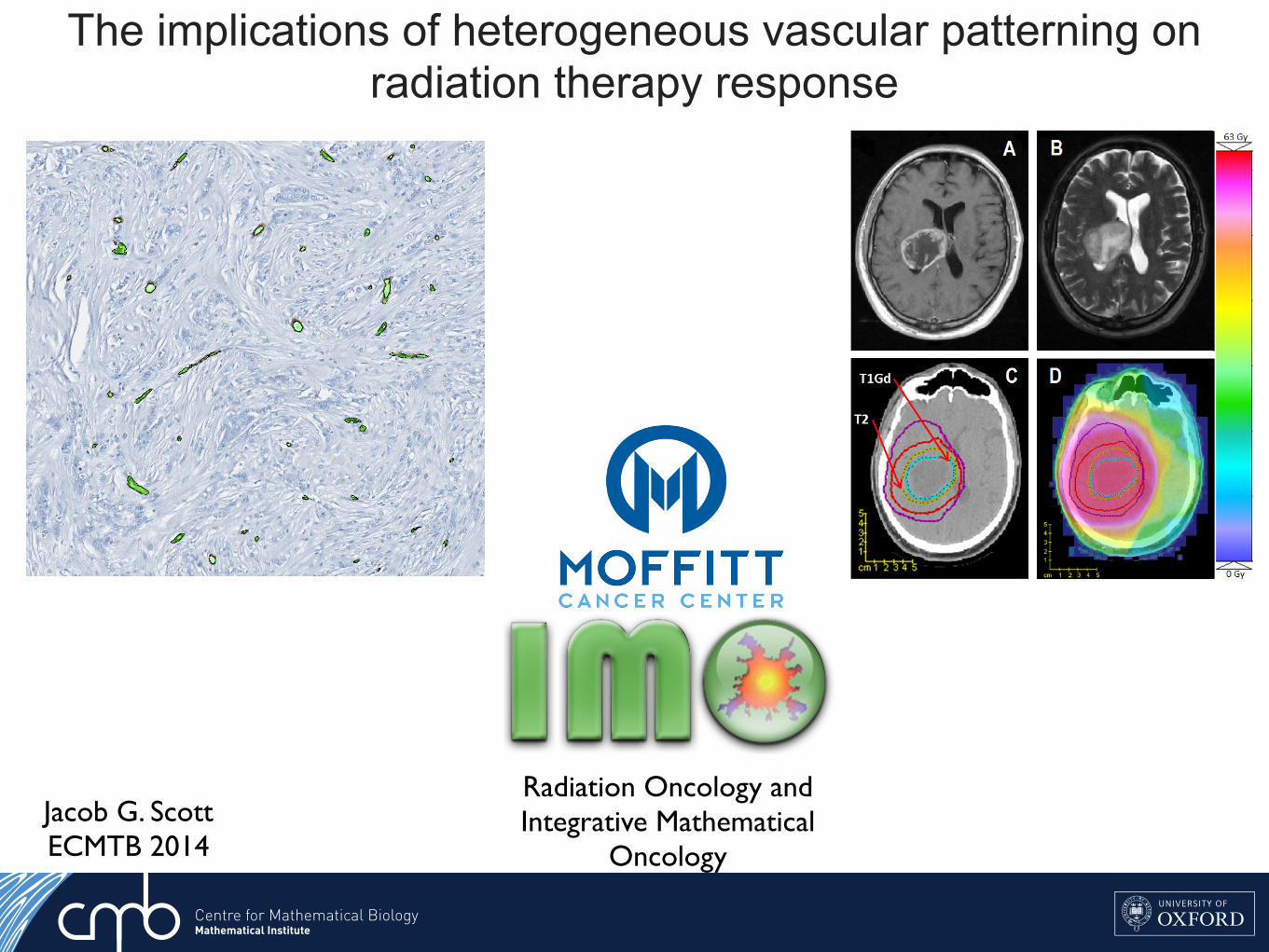
The implications of heterogeneous vascular patterning on radiation therapy response
Jacob G. ScottECMTB 2014
1
Fig 6.
ReferencesWeinberg, R. A. (2007). The biology of cancer. New York: Garland Science. M. Lynch, R. Burger, D. Butcher, and W. Gabriel (1993). The mutational meltdown in asexual populations. J. Hered. 84:339-344.Moran, Patrick Alfred Pierce: The Statistical Processes of Evolutionary Theory. Oxford, Clarendon Press (1962).
Key Factors in the Metastatic Process: Insights from Population Genetics
Christopher McFarland1*, Jacob Scott2,3,*, David Basanta3, Alexander Anderson3, Leonid Mirny1
1Harvard-MIT Division of Health Science & Technology, 2H. Lee Moffitt Cancer and Research Center, 3Integrative Mathematical Oncology, *contributed equally to this work
Fig 1. Prevalence and significance of micrometastases are poorly understood. Most micrometastases never progress to macroscopic size. In this case, small colonies of breast endothelial cells are found in the lung of a non-metastatic breast cancer patient
Background:Metastasis is a highly lethal and poorly understood process that
accounts for the majority cancer deathsPatterns of metastatic spread are not explained by deterministic
explain these patternsWe develop a stochastic model at the genomic level and use
population genetics techniques to explore this phenomenon
Modeling Metastasis:
A tumor was grown in silico by creating a population of single cells that stochastically undergo mitosis and cell death. Cells can gain passenger and driver mutations during division which are passed to their offspring
Results: Effect of primary tumor on Pmet
Success of metastases increases with primary tumor size
Exploring the observed Heterogeneity in genotypes:
We found that Pmet varied considerably between cells from all 100 primary tumors (Left), but less so between cells within the same primary tumor (Right)
Tumors that took longer than the average time to reach 106 cells
Late primary tumors of equivalent size were less likely to metastasize
Clinical Applications:
Modification of the stromal factor could be useful in the mitigation of metastasisThis concept has been shown to be efficacious in the prevention of
Skeletal Related Events (SREs) for prostate and breast cancer metastasis and is the driving concept behind RTOG 0622, a trial of injectable 153Sm for the prevention of bony metastasesThis concept could be applied to other organs for the prevention of
metastases
Conclusions/Future Directions:
Using a genotype scale population genetics model of tumor evolution we have elucidated several factors necessary for successful metastasisFuture directions include testing these predictions against extant
genotype data from primary tumors and metastatic tumors as well as further defining the stromal interaction for different primary tumor types and for different stromas.
Fig 5.
Fig 8.
Fig 7.
Driver Mutation
Passenger Mutation
B(d,p)*
D(N)*
*
Fig. 2
An aliquot of 103 cells was taken from a primary tumor when it reached 5x10⁵ and 106 cells and were then allowed to deposit into a foreign stroma and observed
A stromal penalty s was applied only to driver mutations acquired in the primary tumor because their effects will not be as strong in the new stroma, passenger mutations are not affected by the change in microenvironmentWe then measured the number of secondary tumors that grew into
successful metastases from each aliquot and calculate a probability of metastasis (Pmet)
Fig 3.
NKNDsspdB pp
dd )()1()1(),(
Results: Effect of stromal factor on Pmet
Cells derived from the larger primary tumor succeeded in harsher microenvironmentsMetastatic success is highly dependent upon stromal backgroundThree regimes were observed in the parameter space as s varied, one in which
metastasis was impossible (green), one in which it was certain (yellow) and one in which only cells from certain primary tumor succeed (white)We further define a value, scritical, above which Pmet>50%
Fig 4.
Feature of Model Observed Phenomenon
Population size determined by fitness of cells
Larger Tumors more likely to metastasize
Cells can acquire passenger mutations that are slightly
deleterious
Many micrometastases never grown to macroscopic size
Cells with more mutations are less likely to metastasize
Stromal environment reduces efficacy of driver mutations
Certain stromal conditions prohibit metastasis
Metastasis continues to mutate and evolve
Metastases with same founding cell can have
different fates
Cells divide and acquire mutations on individual basis
Large heterogeneity in probability of metastasis
within primary tumor
No pre-defined growth rate
Late primary tumors less likely to metastasize than early tumors of equivalent
size
100 primary tumors were grown and scritical was calculated for each cell as the tumor grewMedian scritical (blue)
increases with primary tumor sizeThere is significant
heterogeneity of metastatic potential between the individual cells within the tumors as shown by the 5th and 95th percentiles (red) of scritical
Pmet decreases with total number of mutations
We derived a way to calculate Pmet
for every cell in the 100 primary tumors at equivalent sizes when inoculated into a foreign stroma of s = ¾ (not show)Pmet decreased with number of
mutationsThe vast majority of total mutations
are passenger mutations
Fig 6.
Radiation Oncology and Integrative Mathematical
Oncology
tumour center [42]. Progressive Hypoxia from theouter to inner most tumour regions was measured, withthe periphery being normoxic and the core necrotic(Figure 6) . These well recognized features of solidtumours [36, 21, 22, 40] were used to approximatepatient-specific hypoxia.
In the absence of each patients PET scan, macroscopichypoxia across the tumour was approximated usingMRIs. Series of T1Gd MRIs for each patientwere studied, concluding that on average, the coreoccupied 30%, the intermediate region 20% and theperiphery 50% of the total T1Gd visible tumourvolume. These regions were incorporated in the virtualtumour model (Figure 7). The low, intermediate andhigh vascularity voxels from Part 1 were assigned
Figure 5: Patient 4 tumour and dose distribution. A:One slice of the T1Gd MRI. The dark core and lightperiphery can be clearly seen. B: One slice of the T2 MRI.C: Part of the hand-drawn structures matrix, showing theT1Gd and T2 tumour outlines, plus 2 cm margins aroundthem, giving the clinically targetted region. D: A slice ofthe dose distribution. Colormap is given on the right.
to the core, intermediate region and periphery of thetumour. For example, all tumour voxels in the core hadthe stem fraction, Mean pO2 and microscopic hypoxiadistribution of the low vascularity voxel (Table 1 andFigure 2). The CCD for each tumour voxel wasdifferent and depended on the distance of the voxelfrom tumour center of mass (Figure 7).
The core and intermediate region also have a highernumber of stem cells than the periphery [42] which
Figure 6: A T1-Gd enhanced MRI (above) and acartoon (below) showing three distinct regions in thetumour.Above:In a contrast-enhanced T1 tumour, the core is thedarkest region, the periphery a white outline and theintermediate region the transition between core andperiphery. Below: Lack of blood vessels result in chronichypoxia in the core and intermediate region. The colourgradient from dark to light blue shows an increasingoxygen concentration. Source: Persano et al. 2011 [40].
Page 8

Towards patient-specific biology-driven heterogeneous radiation planning: using a computational model of tumor growth to identify
novel radiation sensitivity signatures.Jacob G Scott1,2, David Basanta1, Alex G Fletcher2, Philip K Maini2, Alexander RA Anderson1
1Integrated Mathematical Oncology, H. Lee Moffitt Cancer Center and Research Institute, Tampa, FL2Wolfson Centre for Mathematical Biology, Mathematical Institute, University of Oxford, Oxford, UK
Adapting radiotherapy to hypoxic tumours 4909
Figure 1. Pre- and post-contrast T1-weighted MR images taken in the coronal plane through thehead of the dog with a spontaneous sarcoma. The gross tumour volume (GTV) is enclosed by thewhite contour, while the tongue (T) and mandible (M) are indicated.
This is reflected in figure 2, showing a corresponding image of the tracer concentration inthe tumour. With respect to blood (and thus oxygen) supply, the tumour periphery mayqualitatively be characterized as normoxic, while the core is probably hypoxic or necrotic.
The tentative pO2 distribution (in frequency form) in the canine tumour, as obtained fromthe MR scaling procedure, is given in figure 3. In the same figure, the oxygen distributionobtained from Eppendorf histograph measurements (Brurberg et al 2005) is shown. The two
4910 E Malinen et al
Figure 2. Image of the concentration (in mM) of the contrast agent in the central coronal plane ofthe tumour.
Figure 3. Frequency histograms of the tumour oxygen tension in the canine patient, as determinedby the Eppendorf histograph (Brurberg et al 2005) and the MR analysis.
plots appear similar and rather log-normally distributed, but both have a high frequency ofreadings at the lowest oxygen level. The measured median and mean pO2 levels obtainedfrom the histograph were 8.5 and 13.9 mm Hg, respectively, against 13.6 and 16.6 mm Hg,respectively, estimated from the tentative MR analysis. The correlation coefficient betweenthe histograms was 0.88, and a rank sum test and a Kolmogorov–Smirnov test showed thatthe histograms were not significantly different (p values of 0.20 and 0.14, respectively). The‘hypoxic fraction’, i.e. the fraction of pO2 readings smaller than 5 mm Hg were 0.42 and0.28 for the histograph and MR analysis, respectively. For the current case, it is tentativelyassumed that the MR analysis provides pO2-related images that are biologically relevant.
The compartmental volumes and corresponding mean pO2 levels are given in table 1.In figure 4, coronal images displaying the tumour compartments are shown. It appears thatthe compartmental volumes vary considerably with the coronal plane position although thetumour periphery appears to have higher pO2 levels than the tumour core. As evident, thehypoxic compartments are not spatially continuous, but appear as multiple foci within thegross tumour volume. In figure 5, a 3D reconstruction of hence derived DICOM structure setsused in the treatment planning is displayed.
Biology and microenvironment affect radiation therapy efficacy
Macroscopic hypoxia correlates with radiocontrast uptake, and dose modulation is efficacious, in silico1
In this work, we use a proliferation-invasion-radiotherapy(PIRT) model [7] of GBM growth and response to therapy toaccount for patient-specific tumor proliferation and invasionkinetics combined with a multi-objective evolutionary algorithm(MOEA) for IMRT optimization [8] to demonstrate the potentialto improve tumor control while reducing dose to normal tissuerelative to the standard-of-care. Specifically, we applied themethodology presented in Holdsworth et al (2012) [8] with amore realistic set of optimization inputs, to a cohort of 11 GBMpatients, and compared patient-individualized, optimized IMRTplans with standard-of-care plans. Across this cohort of GBMpatients with diverse imaging patterns, we predicted the benefit ofthe patient-individualized, optimized plans in terms of normaltissue dose, therapeutic ratio and simulated treatment benefit.
Figure 1. Parameter generation for the patient-specific biomathematical model. 1. Determine radial measurements from serial T1Gd andT2/FLAIR magnetic resonance imaging. 2. Compute the invisibility index (D/r) from intra-study T1Gd and T2/FLAIR radial measurements. 3. Computethe radial velocity (2
!!!!!!!Dr
p) from serial T1Gd or T2/FLAIR radial measurements.
doi:10.1371/journal.pone.0079115.g001
Table 1. Optimization Restrictions.
Maximum Fraction/Dose Region
5 Gy Peak Fraction Inside T2/FLAIR
2.5 Gy Peak Fraction Outside T2/FLAIR
65 Gy Peak Dose Outside T2/FLAIR
0.4–1.4 Gy EUD* Fraction Outside T1Gd
*Patient-specific.doi:10.1371/journal.pone.0079115.t001
Patient-Specific Radiotherapy for Glioblastoma
PLOS ONE | www.plosone.org 2 November 2013 | Volume 8 | Issue 11 | e79115
•Radiation dose/fraction is known to depend heavily on local oxygen concentration as well as intrinsic cell parameters•Our ability to quantify these parameters in patients is maturing, but has not translated to the clinic
directly after the scans showed that the i.v.-injected Alexa 680-AC133 mAb had bound to almost all CSC marker-positive cellsin the tumor, verifying that the injected Alexa 680-AC133 mAbhad penetrated the tumor tissue efficiently (Fig. 3E, Left). Toidentify the CSCs ex vivo, the tumor single-cell suspensions werecostained with the AC141 antibody, which is specific for a secondstem cell-specific epitope of CD133. As expected, binding of theinjected Alexa 680-labeled isotype control antibody to CSCs couldnot be detected (Fig. 3E, Right).
FMT Imaging of Intracerebral Xenograft Tumors. Antibodies haveonly limited access to the brain because the undisturbed blood–brain barrier (BBB) is impermeable to macromolecules, andwhether systemically administered antibodies can reach extra-vascular targets in brain tumors with a disturbed BBB is of greatinterest (34, 35). We therefore wanted to find out whether theAC133 mAb is suitable for imaging orthotopically growingAC133+ glioma xenografts. We indeed could detect orthotopicallygrowing NCH421k gliomas noninvasively by NIR FMT imagingupon i.v. injection of the Alexa 680-labeled AC133 mAb (Fig. 3F,Upper Left), and the signal caused by the Alexa 680-AC133 mAb
also could be detected directly postmortem on the excised tu-mor-bearing brains (Fig. 3F, Lower Left).
PET Imaging of Tumor Stem Cell-Derived s.c. Xenografts. After theFMT studies had demonstrated that noninvasive mAb-mediatedvisualization of AC133+ CSCs was possible in principle, we ex-plored immuno-PET detection of AC133+ CSCs. The 64Cu-NOTA-AC133 mAb strongly marked s.c. growing NCH421k gliomas at 24and 48 h postinjection (p.i.) (Fig. 4A, Left and Center), despite theconsiderably lower expression of AC133 on NCH421k cells ascompared with CD133-overexpressing U251 cells (see Fig. 1A andFig. S3A). Particularly remarkable was the much higher tracer up-take liver [an organ exhibiting relatively high unspecific activitybecause of high blood perfusion, antibody metabolism, andpotential transchelation of 64Cu (28, 36)]. The tumor-to-con-tralateral background, tumor-to-blood pool, and tumor-to-livercontrasts were 21.4 ± 8.2, 2.7 ± 0.9, and 2.6 ± 0.8 at 24 h and32.8 ± 19, 6.4 ± 2.5, and 5.4 ± 1.8 at 48 h p.i., respectively. The64Cu-NOTA-isotype control antibody caused only a very weaktumor signal. As judged by visual inspection (Fig. 4A, Right) andaccording to in vivo and in vitro quantification (Fig. 4 B and C),
Fig. 2. PET/CT imaging and biodistribution of 64Cu-NOTA-AC133 mAb in mice bearing s.c. implanted U251 gliomas overexpressing CD133. Nude mice re-ceived !8.0 ± 0.5 MBq 64Cu-NOTA-AC133 mAb via tail vein injection, and PET/CT images were acquired. The mice carried AC133" U251 wild-type and AC133/CD133-overexpressing U251 gliomas in the left and right flanks, respectively. (A) Representative transverse tumor and coronal whole-body PET and fused PET/CT sections at 24 and 48 h p.i. (B) Uptake of 64Cu-NOTA-AC133 mAb as measured by microPET in various organs and AC133" and AC133-overexpressing tumorsat 24 and 48 h p.i. Values are the mean %IA/g of tissue. (C) Ex vivo biodistribution at 24 and 48 h p.i. Values are the mean %IA/g of tissue. n = 7–8 mice pergroup. ***P < 0.001, t test; values represent means ± SD.
Gaedicke et al. PNAS Early Edition | 3 of 10
MED
ICALSC
IENCE
SPN
ASPL
US
1. Malinen et al. Phys Med Biol 2006 2. Corwin et al. PLoS ONE 2013 3. Alfonso et al., PLoS ONE 2014 4. Leder et al, Cell 2014 5. Gaedicke et al., PNAS 2014. 6. Scott et al. PLoS Comp Biol 2014ACKNOWLEDGEMENT: This work sponsored in part by the Moffitt Cancer Center PSOC, NIH/NCI U54CA143970
XRT dose modulation using putative stem distribution3 and dynamics4 shown effective in silico and in vivo4
Cell diffusivity and replication can be inferred from MRI imaging, allowing for understanding of growth prediction and dose shape modification2
Non-invasive PET imaging reported with an anti-body to CD-1335 (putative stem marker)
Several layers of heterogeneity effect radiation efficacy
Figure W7. Segmentation of viable tissue. (A) Representative immunohistochemistry (IHC) staining of pimonidazole in orthotopicMDA-MB-231 tumors from mice given tap water or water containing sodium bicarbonate to drink. (B) Computational segmentationof viable (green) and nonviable (pink) tissues. (C) Positive pixel analysis of segmented viable tissue showing intensity of pimonidazolestaining: blue indicates negative staining, orange indicates moderate staining, and red indicates strong staining.
N
Quantitative Histologyyields vessel organization
Radiomicsyields vessel density
Microenvironmental feedback Lattice based CAStem hierarchy
Non stem-driven tumourhigh vessel density
Stem-driven tumour low vessel densityOxygen concentration (mmHG)
Oxygen concentration (mmHG)
Vess
el D
ensi
ty
TCP
TCP
Oxygen concentration (mmHG)
Oxygen concentration (mmHG)
Tumour control probability depends not only on vessel density, but also on vessel organization
Enabling translation - information from several scales
Optimized plan
Image credit: Unkelbach et al. doi: 10.1088/0031-9155/59/3/771
TCP ~62% TCP ~75%
TCP ~99% TCP ~88%
If I’m not around the poster and you want to chat, this is what I look like. Feel free to contact me at [email protected] or follow on twitter @CancerConnector. You can find this poster on line here: http://dx.doi.org/10.6084/m9.figshare.979442
Mathematical model of a stem driven tumour in a heterogeneous vascular environment6

We use a suite of mathematical and computational models to bridge a range of spatial and temporal scales.
TIME/SPATIAL SCALECELLULAR DETAIL
Evolutionary Game Theory
Reaction Diffusion Models
Hybrid Cellular Automata
Cellular Potts Model
Immersed Boundary ModelHybrid Cellular
AutomataNon-spatial continuum
Reaction Diffusion
Network Theory
represents stem and differentiated cells that are in oxygen concentration j at time t. We
can then represent the suriving fraction after a given single dose (n = 1) of radiation
therapy, by:
N t+1ij = N t
ije−(αijd+βijd2). (2.2)
We have that the total number of surviving cells at time t+ 1 then is
N t+1=
i
j
N t+1ij , (2.3)
which allows us to calculate a VCP of
VCP = e−Nt+1. (2.4)
2.2.2 Dependence of TCP on cell number
It is clear from (2.4) that the VCP depends not only on the actualy oxygen concentration
each cell experiences, but also on the total number of cells. In the following sections we
will explore each of these factors individually, beginning with the number of cells within
a given voxel, which we will call the carrying capacity.
2.2.3 Oxygen dependence
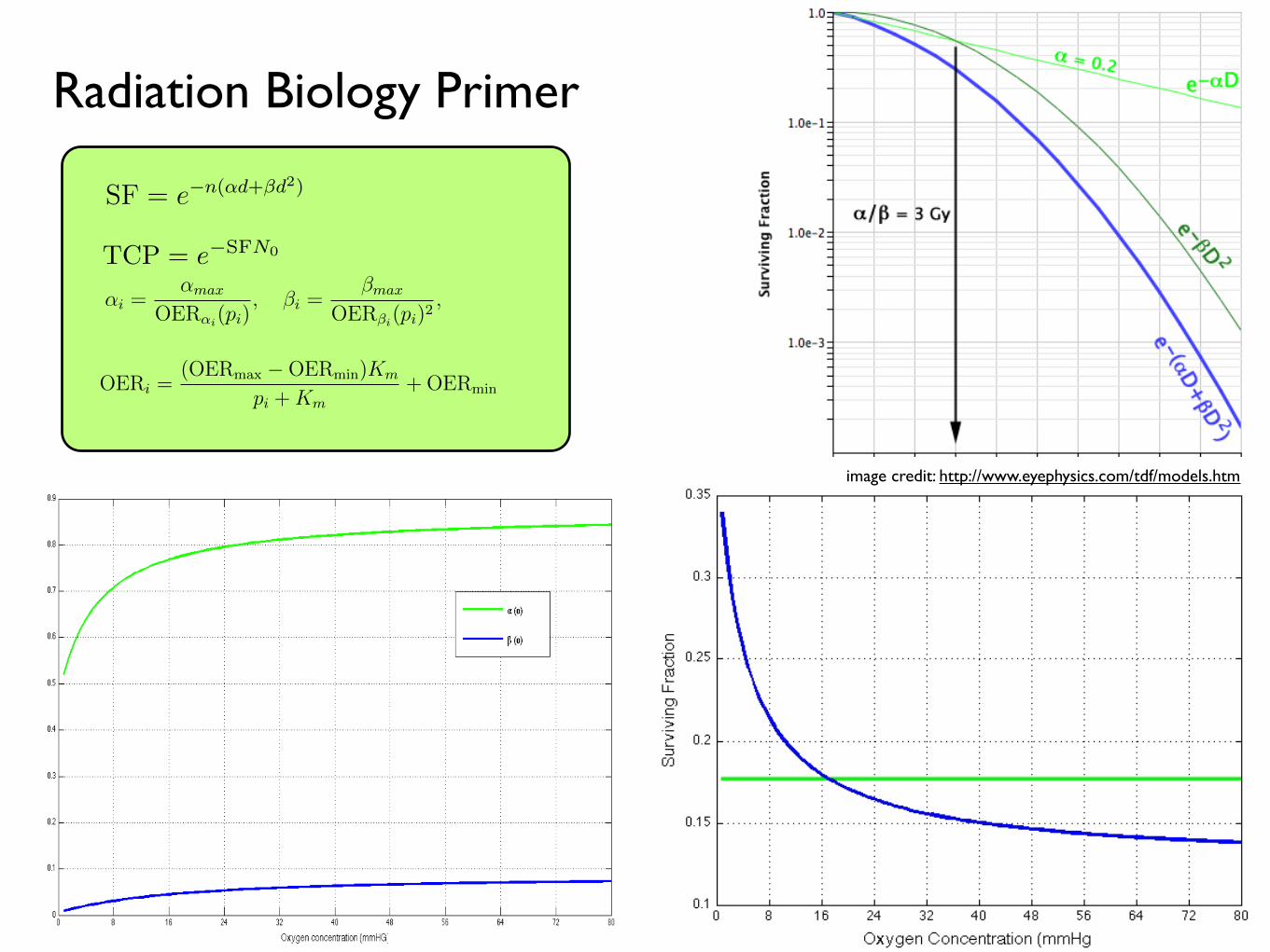
To understand the changes in the radiation parameters, α and β, with oxygen we use the
concept of the oxygen enhancement ratio (OER):
αi =αmax
OERαi(pi), βi =
βmax
OERβi(pi)2, (2.5)
where αmax and βmax are the values of α and β under fully oxygenated conditions and
αi, βi and pi are the values of α, β and oxygen, p, in compartment i. We can further find
the OER as a function of the oxygen concentration by using the relation established by
experimental correlation by Chapman et al. [22], and Palcic and Skarsgard [62]:
OERi =(OERmax −OERmin)Km
pi +Km+OERmin (2.6)
where pi is the oxygen concentration in compartment i,Km = 3.28 and OERαmin =OERβmin =
1 [22, 62, 86]. There is little information about how β changes in glioblastoma with oxy-
gen tension, so for now, we will assume that theαβ ratio for maximally sensitive cells
remains constant at 10 Gy−1 (this is reported in the literature ranging from 8.64 [25] to
XXXXX).
31
represents stem and differentiated cells that are in oxygen concentration j at time t. We
can then represent the suriving fraction after a given single dose (n = 1) of radiation
therapy, by:
N t+1ij = N t
ije−(αijd+βijd2). (2.2)
We have that the total number of surviving cells at time t+ 1 then is
N t+1=
i
j
N t+1ij , (2.3)
which allows us to calculate a VCP of
VCP = e−Nt+1. (2.4)
2.2.2 Dependence of TCP on cell number
It is clear from (2.4) that the VCP depends not only on the actualy oxygen concentration
each cell experiences, but also on the total number of cells. In the following sections we
will explore each of these factors individually, beginning with the number of cells within
a given voxel, which we will call the carrying capacity.
2.2.3 Oxygen dependence
To understand the changes in the radiation parameters, α and β, with oxygen we use the
concept of the oxygen enhancement ratio (OER):
αi =αmax
OERαi(pi), βi =
βmax
OERβi(pi)2, (2.5)
where αmax and βmax are the values of α and β under fully oxygenated conditions and
αi, βi and pi are the values of α, β and oxygen, p, in compartment i. We can further find
the OER as a function of the oxygen concentration by using the relation established by
experimental correlation by Chapman et al. [22], and Palcic and Skarsgard [62]:
OERi =(OERmax −OERmin)Km
pi +Km+OERmin (2.6)
where pi is the oxygen concentration in compartment i,Km = 3.28 and OERαmin =OERβmin =
1 [22, 62, 86]. There is little information about how β changes in glioblastoma with oxy-
gen tension, so for now, we will assume that theαβ ratio for maximally sensitive cells
remains constant at 10 Gy−1 (this is reported in the literature ranging from 8.64 [25] to
XXXXX).
31
model presented in Chapter 2. By identifying broad relationships between in silico tissue
architecture and radiation response, we aim to progress towared a translatable method
of radiation plan optimization from information gleaned from biopsy.
The remainder of this chapter is structured as follows. In Section 2, we provide a
concise summary of the relevant radiation biology, including the relevant equations for
surviving fraction under homogeneous and then heterogeneous oxygen concentrations (the
latter relying on the Oxygen Enhancement Ratio (OER)). In Section 3 we illustrate how
different vascular patterns lead to different numbers of cells and widely varying statistical
properties (no stem hierarchy). In Section 4, we consider a highly simplified scenario with
only two vessels, and define how their relationship in space changes carrying capacity and
also radiation response. In Section 5, we will introduce Riply’s K, a measure of spatial
clumping, and relate this measure, on the domain, with the radiation response. In Section
6, we illustrate how different vascular patterning scenarios would benefit differently from
ordered therapy in the form of vascular normalization therapy and radiation therapy. In
Section 7 we conclude with a summary of work done and discuss potential promisising
avenues for future research in this area.
2.2 Established radiobiology
For this, I will introduce the basics of radiobiological modeling, to include tumor control
probability (TCP), the linear-quadratic model of surviving fraction (SF) [15, 31], the
concepts of oxygen enhancement ratio (OER) and linear energy transfer (LET).
SF = e−n(αd+βd2)(2.1)
where the parameters α and β refer to the radiobiologic parameters associated (phe-
nomenologically) with cell kill secondary to ‘single hit’ events (α) and ‘double hit’ events
(β), d refers to the dose per fraction of radiation and n to the number of fractions.
2.2.1 Tumour control probability
Background on TCP.
While the TCP is a measure that considers the total number of surviving cells in a tumour,
we are interested, in this chapter, in the total number of surviving cells in our domain. We
will therefore derive a measure, based on the TCP, which we will call the Voxel Control
Probability (VCP). To understand the effect of radiation on a distribution of cells, we
consider the individual survival probability of each discrete subpopulation of cells in the
distribution, as characterized by their proliferative state, and their microenvironmental
situation. Specifically, we allow N tij to be the number of cells of type i, where i ∈ S,D
30
image credit: http://www.eyephysics.com/tdf/models.htm
Radiation Biology Primer
TCP = e−SFN0

vessels modelled as point sources of oxygen and an initial field of healthy cells. With
the exception of our previous work [69] this has not been modelled in the context of a
hierarchically organized tumour, but has been shown experimentally to affect the stem
phenotype in vitro [14, 50, 53, 70, 72] and, critically, the response to radiation therapy
[45, 60].
1.2.1 Continuous oxygen field
The continuous component of this model describes the distribution and consumption of
nutrients, which we model as only oxygen. While it is clear that many other chemical
signals are of biological importance, data on the effect of any of these on stem cell-
driven tumours are lacking, making their inclusion difficult. Blood vessels, which are each
modelled as a point source of oxygen occupying one lattice point, are placed randomly
throughout the lattice at the start of a given simulation, with a specified spatial density
Θ. In all simulations we neglect vascular remodelling. Each vessel is assumed to carry an
amount of oxygen equal to that carried in the arterial blood. This oxygen is then allowed
to diffuse into the surrounding tissue.
The spatiotemporal evolution of the oxygen field is described by the reaction-diffusion
partial differential equation (PDE)
∂c(x, t)
∂t= Dc∇2
c(x, t)− fc(x, t), (1.1)
where c(x, t) is the concentration of oxygen at a given time t and position x, Dc is the
diffusion coefficient of oxygen, which we assume to be constant (providing linear, isotropic
diffusion) and fc(x, t) is governed by Michaelis-Menten kinetics and is defined as:
fc(x, t) =
µir(c, t) if there is a cell of type i at x at time t,
0 otherwise,(1.2)
where i ∈ H,S, P, T and the labels H, S, P and T are used to refer to healthy, TIC, TAC
and TD cells respectively. Here µi is defined as the cell type-specific oxygen consumption
constant (µH , µS, µP , µT ), which modulates r(c, t), the oxygen dependent consumption
rate, defined as
r(c, t) = rc
c(x, t)
c(x, t) +Km
where rc and Km denote the maximal uptate rate and effective Michaelis-Menten con-
stant, respectively. We supplement equation (1.1) with the following initial and boundary
conditions. We begin with the oxygen in the domain set to c(x, 0) = c0 and all lattice
points occupied by normal cells. In the case of a cancer simulation, we replace the center
lattice point with a single TIC. Vessels are placed throughout the domain at a prescribed
5
Figure 1.7: Definition of lattice position neighbourhood for cell division (Left) andoxygen diffusion (right). (Left) Cells ascertain whether they have space for division byconsidering the Moore neighbourhood in green. (Right) The oxygen concentration at position(i∆x, j∆x) is calculated using the explicit scheme described in Section 1.2.3.3, considering thevon Neumann neighborhood indicated in yellow and no-flux boundary conditions.
10 cell diameters [33] and the information from the literature concerning the ratio of
cancer to normal oxygen consumption (see Section 1.2.2.1).
Introducing the non-dimensional variables x = x/L, t = t/τ and c = c/c0, we define
the new non-dimensional parameters
Dc =Dcτ
L2, rc =
τn0rcc0
. (1.3)
For notational convenience, we henceforth drop the tildes and refer to the non-dimensional
parameters only as DC and rc. See Table 1.1 for a full list of parameter estimates and
Appendix ?? for our procedure for esimating the cancer cell oxygen consumption rate.
1.2.3.3 Numerical solution
In order to solve equation (1.1) numerically, we discretize space and time by considering
tk = k∆t, xi = i∆x and yj = j∆x and approximate the concentration of oxygen at
timestep k and position (i∆x, j∆x) by cki,j ≈ c(xi, yj, tk). We use a central difference
approximation for the Laplacian and thus approximate equation (1.1) by
ck+1i,j − cki,j
∆t=
DC
∆x2
cki+1,j + cki−1,j + cki,j+1 + cki,j−1 − 4cki,j
−fcki,j, (1.4)
wherefcki,j
is the cell-specific oxygen consumption µcellrc at time k given a cell at
position (i∆x, j∆x) as discussed in equation 1.2. We then rearrange equation (1.4) to
obtain a solution for ck+1i,j , yielding
13
Table 1.1: List of dimensional model parameters and their estimates.
Parameter Meaning Estimate Reference
Dc
Oxygen diffusioncoefficient
1.0× 10⁻⁵cm2s−1 [59]
rcMaximal oxygenconsumption rate
2.3× 10⁻¹⁶mol cells−1 s −1 [32]
c0Background oxygen
concentration1.7× 10−8mol cm −2 [6]
∆xAverage celldiameter
50µm [25]
τAverage celldoubling time
16h [19]
capHypoxicthreshold
0.1 [20]
rpProliferative oxygen
consumption5× rc [32]
Km
Effective Michaelis-Menten constant
0.8mmHg [54]
n0Cancer celldensity
1.6× 10⁵ cells cm −2 [21]
sTIC symmetric
division probability0 ≤ s ≤ 1 Model-specific
aTAC proliferative
capacity0− 10 Model-specific
µcancer/µH
Cancer metabolicratio
2 [12]
ck+1i,j
= cki,j
1− 4
DC∆t
∆x2
+
DC∆t
∆x2
cki+1,j + ck
i−1,j + cki,j+1 + ck
i,j−1
−∆t(fc)
k
i,j. (1.5)
During each update, then, the oxygen tension in a given lattice point is updated
with the values of the surrounding cells using a von Neumann neighbourhood modulated
by the diffusion coefficient, Dc (see Figure 1.7(b)). To impose the zero-flux boundary
conditions we modify equation (1.5) in the case i, j ∈ 1, N. For example, at the
left-hand boundary (i.e. i = 0) we discretize the no-flux boundary condition to obtain
ck0,j = ck2,j, which we substitute into equation (1.5). Lattice points that are occupied by
vessels are excluded from this update as their value never varies from 1.
As a preliminary check of our numerical method, we consider a highly simplified
scenario in which the entire left- and right-hand boundaries of our domain represent
vessels running along the plane. Any horizontal slice through this domain, at a given
time, t, should then approximate the solution to the one-dimensional diffusion equation
14
Diffusion and uptake, exact
Diffusion and uptake, numeric approximation

autophagy (directly translated as ‘self-eating’), a state in which they become resistant
to nutrient starvation [91], and cells are known to die on different time scales and by
different mechanisms (apoptosis vs. necrosis) depending on the magnitude and duration
of the hypoxic insult. While these differences have been shown to affect tumour growth
[19], as this is not the main aim of this model, we will simplify this scenario by assigning
a rate, pd, for cell death at each cellular automaton update defined in Section 2.2.3, when
under extreme hypoxia (i.e. c < cap).
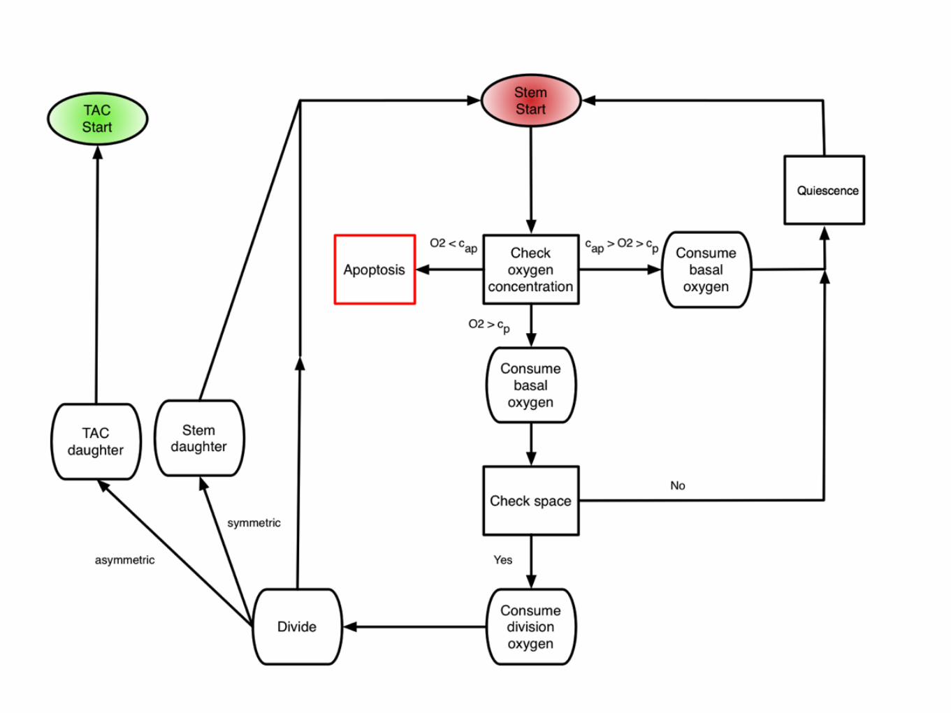
2.2.2.4 Quiescence
When cells sense that there is not enough oxygen to divide, or experience contact inhi-
bition, they undergo a state of quiescence during which there is no division. We model
this as an oxygen threshold (c < cp) below which cellular division is not possible and by
the spatial constraint which requires the cell to be quiescent if there is not at least one
neighbouring lattice point (Moore neighbourhood, see Figure 2.7(a)) empty or inhabited
by a normal cell. When a cell senses that sufficient oxygen and a neighbouring site have
become available, the state of quiescence is reversed.
Figure 2.3: A summary of oxygen based cell fate threshholds. At each cellular au-tomaton update, each cell in the domain undergoes a series of fate decisions based on the localoxygen concentration. When c < cap, cells die at rate pd, when cap < c < cp cells are quiescentand then c > cp cells are capable of proliferation, given all other constraints are met.
2.2.2.5 Normal tissue approximation
The invasion of cancer cells into healthy tissue has been widely studied [7, 38, 39, 42, 70].
While this process is not the focus of our study, we nevertheless must consider the healthy
tissue surrounding our growing tumour, as it plays an important role in modulating
the local oxygen concentration. Previous investigations have modelled tumour spheroid
growth [17, 25, 43, 86], or assumed a constant influx of oxygen from the boundary of
the tissue [42, 81], but as we endeavour to understand how heterogeneous vascularization
affects the growth of a TIC-driven tumour, we must also incorporate normal tissue effects.
To do this, we make the assumption that the entire field is initially comprised of normal
cells, which can divide if they have sufficient space, which consume oxygen at a rate of
10

Dom
ain
Size
Healthy tissue with regular vascular patterning
1 2 3
4 5
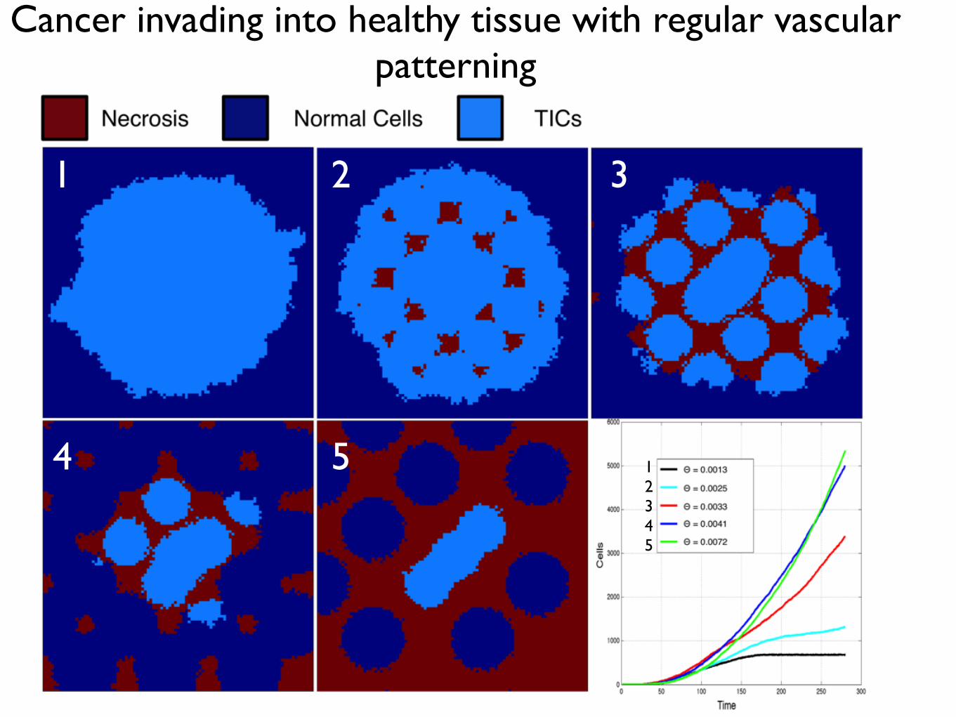
Cancer invading into healthy tissue with regular vascular patterning
12345

Cancer invading into normal tissue with irregular patterning
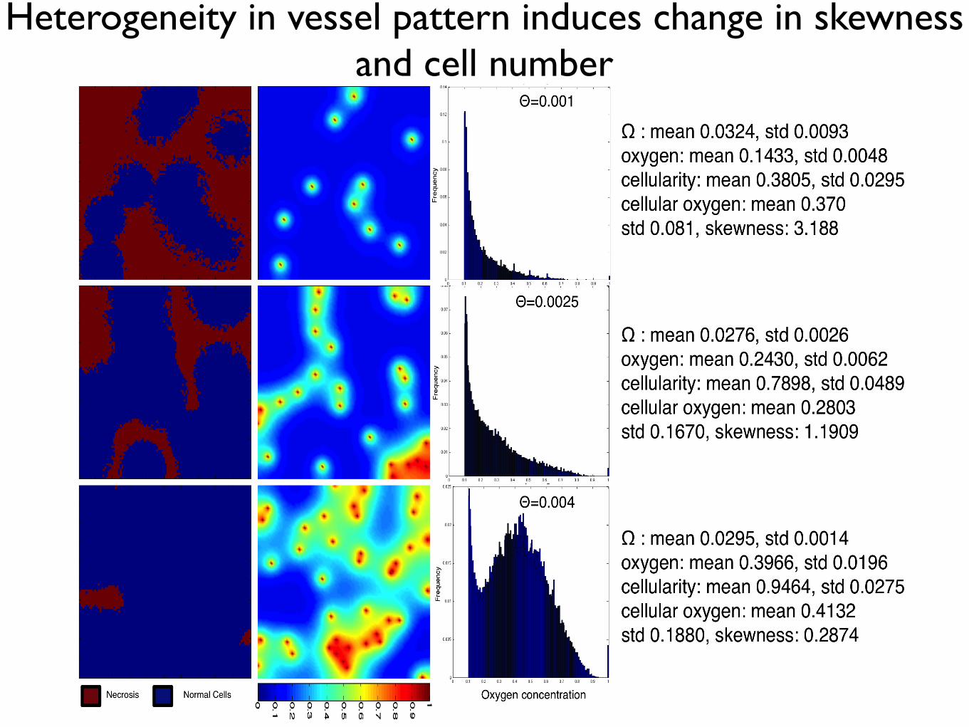
Figure 1.11: Varying vascular density affects the carrying capacity of normal tissueand the cell-oxygen concentration distribution. We show the results of normal tissuegrowth and maintenance as we increase the number of randomly seeded vessels from 10 (top)to 25 (middle) to 40 (bottom). Cells (left) and oxygen concentration (centre) are visualized.We plot the average distribution of healthy cells by oxygen concentration (Right) over ten runsof the simulation with different vascular distributions but constant number of vessels. Everysimulation ends in a dynamic equilibrium (after 200 timesteps, see Appendix ??).
the resulting healthy tissue growth and maintenance in a variety of vascular patterns of
the same density (Figure 1.11). We plot the final, stable distribution of healthy cells for
a random placement of vessels for a given density (Θ = 0.001, top, Θ = 0.0025, middle,
and Θ = 0.004 bottom) in the left and middle columns. In the right column, we plot the
average distribution of cells at specific oxygen concentration over ten simuluations with
different vascular patterns.
As expected, we see an increase in carrying capacity with increasing vascular density
like in the regularly vascularized scenario with mean cellularity increasing from 0.3445−0.9424 with standard deviations from 0.0208−0.0312. Over the ten simulations, we find a
consistent results in each case for aggregation coefficient ranging from Ω = 0.0285−0.0303
with standard deviations from 0.0012− 0.0047, but we find striking differences from the
regularly vascularized case in the distribution of cell-specific oxygen concentration (Figure
1.11) - right). While in the regular case (Figure 1.9) we find conserved cellular-oxygen
distribution shapes (second and third moments), in the irregularly vascularized case we
find two changes: first, even in the highest vessel density there is a large peak at cap and
20
Heterogeneity in vessel pattern induces change in skewness and cell number

Simplest scenario, two vessels

500 simulations of small domain at dynamic equilibriumwith N randomly seeded vessels
N/(domain size)
Cel
l den
sity

Towards patient-specific biology-driven heterogeneous radiation planning: using a computational model of tumor growth to identify
novel radiation sensitivity signatures.Jacob G Scott1,2, David Basanta1, Alex G Fletcher2, Philip K Maini2, Alexander RA Anderson1
1Integrated Mathematical Oncology, H. Lee Moffitt Cancer Center and Research Institute, Tampa, FL2Wolfson Centre for Mathematical Biology, Mathematical Institute, University of Oxford, Oxford, UK
Adapting radiotherapy to hypoxic tumours 4909
Figure 1. Pre- and post-contrast T1-weighted MR images taken in the coronal plane through thehead of the dog with a spontaneous sarcoma. The gross tumour volume (GTV) is enclosed by thewhite contour, while the tongue (T) and mandible (M) are indicated.
This is reflected in figure 2, showing a corresponding image of the tracer concentration inthe tumour. With respect to blood (and thus oxygen) supply, the tumour periphery mayqualitatively be characterized as normoxic, while the core is probably hypoxic or necrotic.
The tentative pO2 distribution (in frequency form) in the canine tumour, as obtained fromthe MR scaling procedure, is given in figure 3. In the same figure, the oxygen distributionobtained from Eppendorf histograph measurements (Brurberg et al 2005) is shown. The two
4910 E Malinen et al
Figure 2. Image of the concentration (in mM) of the contrast agent in the central coronal plane ofthe tumour.
Figure 3. Frequency histograms of the tumour oxygen tension in the canine patient, as determinedby the Eppendorf histograph (Brurberg et al 2005) and the MR analysis.
plots appear similar and rather log-normally distributed, but both have a high frequency ofreadings at the lowest oxygen level. The measured median and mean pO2 levels obtainedfrom the histograph were 8.5 and 13.9 mm Hg, respectively, against 13.6 and 16.6 mm Hg,respectively, estimated from the tentative MR analysis. The correlation coefficient betweenthe histograms was 0.88, and a rank sum test and a Kolmogorov–Smirnov test showed thatthe histograms were not significantly different (p values of 0.20 and 0.14, respectively). The‘hypoxic fraction’, i.e. the fraction of pO2 readings smaller than 5 mm Hg were 0.42 and0.28 for the histograph and MR analysis, respectively. For the current case, it is tentativelyassumed that the MR analysis provides pO2-related images that are biologically relevant.
The compartmental volumes and corresponding mean pO2 levels are given in table 1.In figure 4, coronal images displaying the tumour compartments are shown. It appears thatthe compartmental volumes vary considerably with the coronal plane position although thetumour periphery appears to have higher pO2 levels than the tumour core. As evident, thehypoxic compartments are not spatially continuous, but appear as multiple foci within thegross tumour volume. In figure 5, a 3D reconstruction of hence derived DICOM structure setsused in the treatment planning is displayed.
Biology and microenvironment affect radiation therapy efficacy
Macroscopic hypoxia correlates with radiocontrast uptake, and dose modulation is efficacious, in silico1
In this work, we use a proliferation-invasion-radiotherapy(PIRT) model [7] of GBM growth and response to therapy toaccount for patient-specific tumor proliferation and invasionkinetics combined with a multi-objective evolutionary algorithm(MOEA) for IMRT optimization [8] to demonstrate the potentialto improve tumor control while reducing dose to normal tissuerelative to the standard-of-care. Specifically, we applied themethodology presented in Holdsworth et al (2012) [8] with amore realistic set of optimization inputs, to a cohort of 11 GBMpatients, and compared patient-individualized, optimized IMRTplans with standard-of-care plans. Across this cohort of GBMpatients with diverse imaging patterns, we predicted the benefit ofthe patient-individualized, optimized plans in terms of normaltissue dose, therapeutic ratio and simulated treatment benefit.
Figure 1. Parameter generation for the patient-specific biomathematical model. 1. Determine radial measurements from serial T1Gd andT2/FLAIR magnetic resonance imaging. 2. Compute the invisibility index (D/r) from intra-study T1Gd and T2/FLAIR radial measurements. 3. Computethe radial velocity (2
!!!!!!!Dr
p) from serial T1Gd or T2/FLAIR radial measurements.
doi:10.1371/journal.pone.0079115.g001
Table 1. Optimization Restrictions.
Maximum Fraction/Dose Region
5 Gy Peak Fraction Inside T2/FLAIR
2.5 Gy Peak Fraction Outside T2/FLAIR
65 Gy Peak Dose Outside T2/FLAIR
0.4–1.4 Gy EUD* Fraction Outside T1Gd
*Patient-specific.doi:10.1371/journal.pone.0079115.t001
Patient-Specific Radiotherapy for Glioblastoma
PLOS ONE | www.plosone.org 2 November 2013 | Volume 8 | Issue 11 | e79115
•Radiation dose/fraction is known to depend heavily on local oxygen concentration as well as intrinsic cell parameters•Our ability to quantify these parameters in patients is maturing, but has not translated to the clinic
directly after the scans showed that the i.v.-injected Alexa 680-AC133 mAb had bound to almost all CSC marker-positive cellsin the tumor, verifying that the injected Alexa 680-AC133 mAbhad penetrated the tumor tissue efficiently (Fig. 3E, Left). Toidentify the CSCs ex vivo, the tumor single-cell suspensions werecostained with the AC141 antibody, which is specific for a secondstem cell-specific epitope of CD133. As expected, binding of theinjected Alexa 680-labeled isotype control antibody to CSCs couldnot be detected (Fig. 3E, Right).
FMT Imaging of Intracerebral Xenograft Tumors. Antibodies haveonly limited access to the brain because the undisturbed blood–brain barrier (BBB) is impermeable to macromolecules, andwhether systemically administered antibodies can reach extra-vascular targets in brain tumors with a disturbed BBB is of greatinterest (34, 35). We therefore wanted to find out whether theAC133 mAb is suitable for imaging orthotopically growingAC133+ glioma xenografts. We indeed could detect orthotopicallygrowing NCH421k gliomas noninvasively by NIR FMT imagingupon i.v. injection of the Alexa 680-labeled AC133 mAb (Fig. 3F,Upper Left), and the signal caused by the Alexa 680-AC133 mAb
also could be detected directly postmortem on the excised tu-mor-bearing brains (Fig. 3F, Lower Left).
PET Imaging of Tumor Stem Cell-Derived s.c. Xenografts. After theFMT studies had demonstrated that noninvasive mAb-mediatedvisualization of AC133+ CSCs was possible in principle, we ex-plored immuno-PET detection of AC133+ CSCs. The 64Cu-NOTA-AC133 mAb strongly marked s.c. growing NCH421k gliomas at 24and 48 h postinjection (p.i.) (Fig. 4A, Left and Center), despite theconsiderably lower expression of AC133 on NCH421k cells ascompared with CD133-overexpressing U251 cells (see Fig. 1A andFig. S3A). Particularly remarkable was the much higher tracer up-take liver [an organ exhibiting relatively high unspecific activitybecause of high blood perfusion, antibody metabolism, andpotential transchelation of 64Cu (28, 36)]. The tumor-to-con-tralateral background, tumor-to-blood pool, and tumor-to-livercontrasts were 21.4 ± 8.2, 2.7 ± 0.9, and 2.6 ± 0.8 at 24 h and32.8 ± 19, 6.4 ± 2.5, and 5.4 ± 1.8 at 48 h p.i., respectively. The64Cu-NOTA-isotype control antibody caused only a very weaktumor signal. As judged by visual inspection (Fig. 4A, Right) andaccording to in vivo and in vitro quantification (Fig. 4 B and C),
Fig. 2. PET/CT imaging and biodistribution of 64Cu-NOTA-AC133 mAb in mice bearing s.c. implanted U251 gliomas overexpressing CD133. Nude mice re-ceived !8.0 ± 0.5 MBq 64Cu-NOTA-AC133 mAb via tail vein injection, and PET/CT images were acquired. The mice carried AC133" U251 wild-type and AC133/CD133-overexpressing U251 gliomas in the left and right flanks, respectively. (A) Representative transverse tumor and coronal whole-body PET and fused PET/CT sections at 24 and 48 h p.i. (B) Uptake of 64Cu-NOTA-AC133 mAb as measured by microPET in various organs and AC133" and AC133-overexpressing tumorsat 24 and 48 h p.i. Values are the mean %IA/g of tissue. (C) Ex vivo biodistribution at 24 and 48 h p.i. Values are the mean %IA/g of tissue. n = 7–8 mice pergroup. ***P < 0.001, t test; values represent means ± SD.
Gaedicke et al. PNAS Early Edition | 3 of 10
MED
ICALSC
IENCE
SPN
ASPL
US
1. Malinen et al. Phys Med Biol 2006 2. Corwin et al. PLoS ONE 2013 3. Alfonso et al., PLoS ONE 2014 4. Leder et al, Cell 2014 5. Gaedicke et al., PNAS 2014. 6. Scott et al. PLoS Comp Biol 2014ACKNOWLEDGEMENT: This work sponsored in part by the Moffitt Cancer Center PSOC, NIH/NCI U54CA143970
XRT dose modulation using putative stem distribution3 and dynamics4 shown effective in silico and in vivo4
Cell diffusivity and replication can be inferred from MRI imaging, allowing for understanding of growth prediction and dose shape modification2
Non-invasive PET imaging reported with an anti-body to CD-1335 (putative stem marker)
Several layers of heterogeneity effect radiation efficacy
Figure W7. Segmentation of viable tissue. (A) Representative immunohistochemistry (IHC) staining of pimonidazole in orthotopicMDA-MB-231 tumors from mice given tap water or water containing sodium bicarbonate to drink. (B) Computational segmentationof viable (green) and nonviable (pink) tissues. (C) Positive pixel analysis of segmented viable tissue showing intensity of pimonidazolestaining: blue indicates negative staining, orange indicates moderate staining, and red indicates strong staining.
N
Quantitative Histologyyields vessel organization
Radiomicsyields vessel density
Microenvironmental feedback Lattice based CAStem hierarchy
Non stem-driven tumourhigh vessel density
Stem-driven tumour low vessel densityOxygen concentration (mmHG)
Oxygen concentration (mmHG)
Vess
el D
ensi
ty
TCP
TCP
Oxygen concentration (mmHG)
Oxygen concentration (mmHG)
Tumour control probability depends not only on vessel density, but also on vessel organization
Enabling translation - information from several scales
Optimized plan
Image credit: Unkelbach et a. doi: 10.1088/0031-9155/59/3/771
TCP ~62% TCP ~75%
TCP ~99% TCP ~88%
If I’m not around the poster and you want to chat, this is what I look like. Feel free to contact me at [email protected] or follow on twitter @CancerConnector. You can find this poster
on line here:
Mathematical model of a stem driven tumour in a heterogeneous vascular environment6
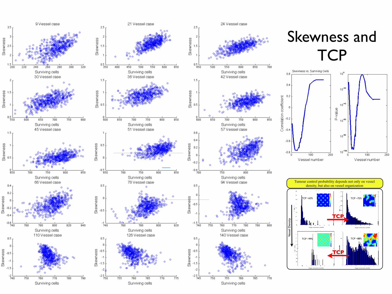
Skewness and TCP
Towards patient-specific biology-driven heterogeneous radiation planning: using a computational model of tumor growth to identify
novel radiation sensitivity signatures.Jacob G Scott1,2, David Basanta1, Alex G Fletcher2, Philip K Maini2, Alexander RA Anderson1
1Integrated Mathematical Oncology, H. Lee Moffitt Cancer Center and Research Institute, Tampa, FL2Wolfson Centre for Mathematical Biology, Mathematical Institute, University of Oxford, Oxford, UK
Adapting radiotherapy to hypoxic tumours 4909
Figure 1. Pre- and post-contrast T1-weighted MR images taken in the coronal plane through thehead of the dog with a spontaneous sarcoma. The gross tumour volume (GTV) is enclosed by thewhite contour, while the tongue (T) and mandible (M) are indicated.
This is reflected in figure 2, showing a corresponding image of the tracer concentration inthe tumour. With respect to blood (and thus oxygen) supply, the tumour periphery mayqualitatively be characterized as normoxic, while the core is probably hypoxic or necrotic.
The tentative pO2 distribution (in frequency form) in the canine tumour, as obtained fromthe MR scaling procedure, is given in figure 3. In the same figure, the oxygen distributionobtained from Eppendorf histograph measurements (Brurberg et al 2005) is shown. The two
4910 E Malinen et al
Figure 2. Image of the concentration (in mM) of the contrast agent in the central coronal plane ofthe tumour.
Figure 3. Frequency histograms of the tumour oxygen tension in the canine patient, as determinedby the Eppendorf histograph (Brurberg et al 2005) and the MR analysis.
plots appear similar and rather log-normally distributed, but both have a high frequency ofreadings at the lowest oxygen level. The measured median and mean pO2 levels obtainedfrom the histograph were 8.5 and 13.9 mm Hg, respectively, against 13.6 and 16.6 mm Hg,respectively, estimated from the tentative MR analysis. The correlation coefficient betweenthe histograms was 0.88, and a rank sum test and a Kolmogorov–Smirnov test showed thatthe histograms were not significantly different (p values of 0.20 and 0.14, respectively). The‘hypoxic fraction’, i.e. the fraction of pO2 readings smaller than 5 mm Hg were 0.42 and0.28 for the histograph and MR analysis, respectively. For the current case, it is tentativelyassumed that the MR analysis provides pO2-related images that are biologically relevant.
The compartmental volumes and corresponding mean pO2 levels are given in table 1.In figure 4, coronal images displaying the tumour compartments are shown. It appears thatthe compartmental volumes vary considerably with the coronal plane position although thetumour periphery appears to have higher pO2 levels than the tumour core. As evident, thehypoxic compartments are not spatially continuous, but appear as multiple foci within thegross tumour volume. In figure 5, a 3D reconstruction of hence derived DICOM structure setsused in the treatment planning is displayed.
Biology and microenvironment affect radiation therapy efficacy
Macroscopic hypoxia correlates with radiocontrast uptake, and dose modulation is efficacious, in silico1
In this work, we use a proliferation-invasion-radiotherapy(PIRT) model [7] of GBM growth and response to therapy toaccount for patient-specific tumor proliferation and invasionkinetics combined with a multi-objective evolutionary algorithm(MOEA) for IMRT optimization [8] to demonstrate the potentialto improve tumor control while reducing dose to normal tissuerelative to the standard-of-care. Specifically, we applied themethodology presented in Holdsworth et al (2012) [8] with amore realistic set of optimization inputs, to a cohort of 11 GBMpatients, and compared patient-individualized, optimized IMRTplans with standard-of-care plans. Across this cohort of GBMpatients with diverse imaging patterns, we predicted the benefit ofthe patient-individualized, optimized plans in terms of normaltissue dose, therapeutic ratio and simulated treatment benefit.
Figure 1. Parameter generation for the patient-specific biomathematical model. 1. Determine radial measurements from serial T1Gd andT2/FLAIR magnetic resonance imaging. 2. Compute the invisibility index (D/r) from intra-study T1Gd and T2/FLAIR radial measurements. 3. Computethe radial velocity (2
!!!!!!!Dr
p) from serial T1Gd or T2/FLAIR radial measurements.
doi:10.1371/journal.pone.0079115.g001
Table 1. Optimization Restrictions.
Maximum Fraction/Dose Region
5 Gy Peak Fraction Inside T2/FLAIR
2.5 Gy Peak Fraction Outside T2/FLAIR
65 Gy Peak Dose Outside T2/FLAIR
0.4–1.4 Gy EUD* Fraction Outside T1Gd
*Patient-specific.doi:10.1371/journal.pone.0079115.t001
Patient-Specific Radiotherapy for Glioblastoma
PLOS ONE | www.plosone.org 2 November 2013 | Volume 8 | Issue 11 | e79115
•Radiation dose/fraction is known to depend heavily on local oxygen concentration as well as intrinsic cell parameters•Our ability to quantify these parameters in patients is maturing, but has not translated to the clinic
directly after the scans showed that the i.v.-injected Alexa 680-AC133 mAb had bound to almost all CSC marker-positive cellsin the tumor, verifying that the injected Alexa 680-AC133 mAbhad penetrated the tumor tissue efficiently (Fig. 3E, Left). Toidentify the CSCs ex vivo, the tumor single-cell suspensions werecostained with the AC141 antibody, which is specific for a secondstem cell-specific epitope of CD133. As expected, binding of theinjected Alexa 680-labeled isotype control antibody to CSCs couldnot be detected (Fig. 3E, Right).
FMT Imaging of Intracerebral Xenograft Tumors. Antibodies haveonly limited access to the brain because the undisturbed blood–brain barrier (BBB) is impermeable to macromolecules, andwhether systemically administered antibodies can reach extra-vascular targets in brain tumors with a disturbed BBB is of greatinterest (34, 35). We therefore wanted to find out whether theAC133 mAb is suitable for imaging orthotopically growingAC133+ glioma xenografts. We indeed could detect orthotopicallygrowing NCH421k gliomas noninvasively by NIR FMT imagingupon i.v. injection of the Alexa 680-labeled AC133 mAb (Fig. 3F,Upper Left), and the signal caused by the Alexa 680-AC133 mAb
also could be detected directly postmortem on the excised tu-mor-bearing brains (Fig. 3F, Lower Left).
PET Imaging of Tumor Stem Cell-Derived s.c. Xenografts. After theFMT studies had demonstrated that noninvasive mAb-mediatedvisualization of AC133+ CSCs was possible in principle, we ex-plored immuno-PET detection of AC133+ CSCs. The 64Cu-NOTA-AC133 mAb strongly marked s.c. growing NCH421k gliomas at 24and 48 h postinjection (p.i.) (Fig. 4A, Left and Center), despite theconsiderably lower expression of AC133 on NCH421k cells ascompared with CD133-overexpressing U251 cells (see Fig. 1A andFig. S3A). Particularly remarkable was the much higher tracer up-take liver [an organ exhibiting relatively high unspecific activitybecause of high blood perfusion, antibody metabolism, andpotential transchelation of 64Cu (28, 36)]. The tumor-to-con-tralateral background, tumor-to-blood pool, and tumor-to-livercontrasts were 21.4 ± 8.2, 2.7 ± 0.9, and 2.6 ± 0.8 at 24 h and32.8 ± 19, 6.4 ± 2.5, and 5.4 ± 1.8 at 48 h p.i., respectively. The64Cu-NOTA-isotype control antibody caused only a very weaktumor signal. As judged by visual inspection (Fig. 4A, Right) andaccording to in vivo and in vitro quantification (Fig. 4 B and C),
Fig. 2. PET/CT imaging and biodistribution of 64Cu-NOTA-AC133 mAb in mice bearing s.c. implanted U251 gliomas overexpressing CD133. Nude mice re-ceived !8.0 ± 0.5 MBq 64Cu-NOTA-AC133 mAb via tail vein injection, and PET/CT images were acquired. The mice carried AC133" U251 wild-type and AC133/CD133-overexpressing U251 gliomas in the left and right flanks, respectively. (A) Representative transverse tumor and coronal whole-body PET and fused PET/CT sections at 24 and 48 h p.i. (B) Uptake of 64Cu-NOTA-AC133 mAb as measured by microPET in various organs and AC133" and AC133-overexpressing tumorsat 24 and 48 h p.i. Values are the mean %IA/g of tissue. (C) Ex vivo biodistribution at 24 and 48 h p.i. Values are the mean %IA/g of tissue. n = 7–8 mice pergroup. ***P < 0.001, t test; values represent means ± SD.
Gaedicke et al. PNAS Early Edition | 3 of 10
MED
ICALSC
IENCE
SPN
ASPL
US
1. Malinen et al. Phys Med Biol 2006 2. Corwin et al. PLoS ONE 2013 3. Alfonso et al., PLoS ONE 2014 4. Leder et al, Cell 2014 5. Gaedicke et al., PNAS 2014. 6. Scott et al. PLoS Comp Biol 2014ACKNOWLEDGEMENT: This work sponsored in part by the Moffitt Cancer Center PSOC, NIH/NCI U54CA143970
XRT dose modulation using putative stem distribution3 and dynamics4 shown effective in silico and in vivo4
Cell diffusivity and replication can be inferred from MRI imaging, allowing for understanding of growth prediction and dose shape modification2
Non-invasive PET imaging reported with an anti-body to CD-1335 (putative stem marker)
Several layers of heterogeneity effect radiation efficacy
Figure W7. Segmentation of viable tissue. (A) Representative immunohistochemistry (IHC) staining of pimonidazole in orthotopicMDA-MB-231 tumors from mice given tap water or water containing sodium bicarbonate to drink. (B) Computational segmentationof viable (green) and nonviable (pink) tissues. (C) Positive pixel analysis of segmented viable tissue showing intensity of pimonidazolestaining: blue indicates negative staining, orange indicates moderate staining, and red indicates strong staining.
N
Quantitative Histologyyields vessel organization
Radiomicsyields vessel density
Microenvironmental feedback Lattice based CAStem hierarchy
Non stem-driven tumourhigh vessel density
Stem-driven tumour low vessel densityOxygen concentration (mmHG)
Oxygen concentration (mmHG)
Vess
el D
ensi
ty
TCP
TCP
Oxygen concentration (mmHG)
Oxygen concentration (mmHG)
Tumour control probability depends not only on vessel density, but also on vessel organization
Enabling translation - information from several scales
Optimized plan
Image credit: Unkelbach et a. doi: 10.1088/0031-9155/59/3/771
TCP ~62% TCP ~75%
TCP ~99% TCP ~88%
If I’m not around the poster and you want to chat, this is what I look like. Feel free to contact me at [email protected] or follow on twitter @CancerConnector. You can find this poster
on line here:
Mathematical model of a stem driven tumour in a heterogeneous vascular environment6


Ripley’s K(t)Figure 3.3: Proportion of simulations (from Figure 3.2) that yield a cell density greater than90%, exhibiting a sigmoid shape.
of spatial units indexed by i and j, X is the variable of interest, in this case oxygen
concentration and X is the global mean of X. The matrix w is a matrix that contains
spatial weights which take the value of 1 if the elements i and j are adjacent, and 0
otherwise.
While this measure is useful in a number of ecological contexts, for our purposes it is
not. As suggested by Legendre et al. CITE, the residual spatial autocorrelation between
cells and oxygen, and the short relative length scale on which oxygen varies as compared
to vessel presence/absence, makes all landscapes appear to be well correlated, that is,
have a Moran’s I measure that approaches zero.
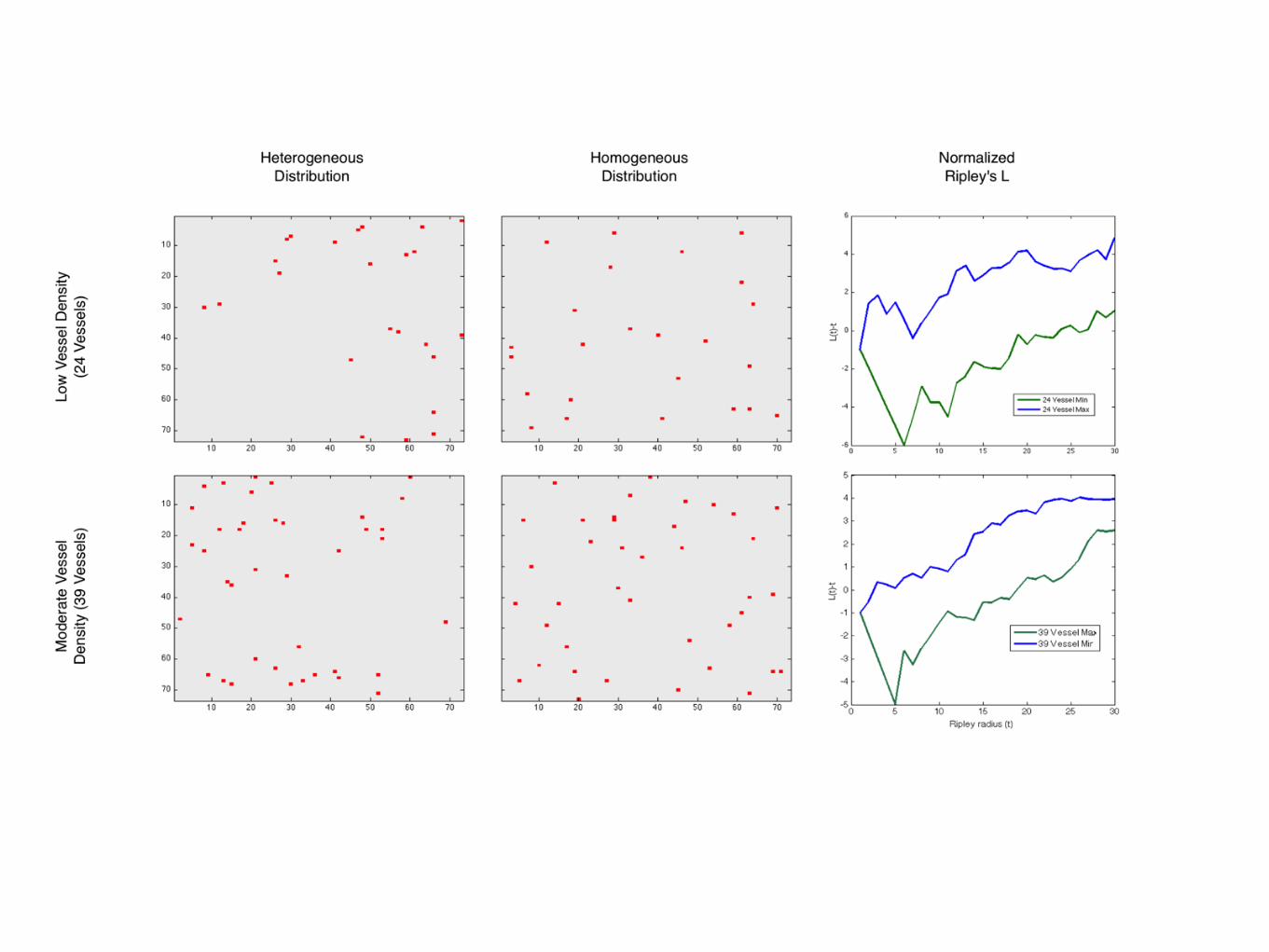
3.5.2.2 Ripley’s K
A more appropriate measure is Ripley’s K, and its variance stabilized cousin, Ripley’s
L. These measures, which are functions of distance, describe, instead of adjacent elements,
the number of elements within a given distance. For Ripley’s K, we have
K(t) = λ−1
i =j
I(dij < t)
n, (3.8)
where λ is the average density of points in the domain, I is the indicator function which
yields
I(dij < t) =
1 if the Euclidian distance fromi → j < t,
0 otherwise.(3.9)
We will utilize the variance stabilized version of this measure, L(t) which is given by
35
Figure 3.3: Proportion of simulations (from Figure 3.2) that yield a cell density greater than90%, exhibiting a sigmoid shape.
of spatial units indexed by i and j, X is the variable of interest, in this case oxygen
concentration and X is the global mean of X. The matrix w is a matrix that contains
spatial weights which take the value of 1 if the elements i and j are adjacent, and 0
otherwise.
While this measure is useful in a number of ecological contexts, for our purposes it is
not. As suggested by Legendre et al. CITE, the residual spatial autocorrelation between
cells and oxygen, and the short relative length scale on which oxygen varies as compared
to vessel presence/absence, makes all landscapes appear to be well correlated, that is,
have a Moran’s I measure that approaches zero.
3.5.2.2 Ripley’s K
A more appropriate measure is Ripley’s K, and its variance stabilized cousin, Ripley’s
L. These measures, which are functions of distance, describe, instead of adjacent elements,
the number of elements within a given distance. For Ripley’s K, we have
K(t) = λ−1
i =j
I(dij < t)
n, (3.8)
where λ is the average density of points in the domain, I is the indicator function which
yields
I(dij < t) =
1 if the Euclidian distance fromi → j < t,
0 otherwise.(3.9)
We will utilize the variance stabilized version of this measure, L(t) which is given by
35
Figure 3.4: Our assumptions about cellular oxygen distributions give rise to dif-
ferences in tumour control probability. We plot two different test distributions,
uniform (Left) and Poisson (center) and compare these to actual data taken from
the CA (right). Each distribution is mapped on to the same number of cells and
the TCP is calculated as per equation (3.6). The Poisson distribution was generated
using a lambda value eqivalent to the mean of the measured distribution from the
CA. The CA distribution was created by averaging 200 time points of data from
the CA after it reached dynamic equilibrium. We find quite different TCPs, 87%,
99% and 91%, respectively.
L(t) =K(t)
π
1/2
, (3.10)
which has an expected value of L(t) = t for homogeneous data. To correct for edge
effects, we implement the correction suggested by Ripley (CITE), which changes the
value of the indicator function, for points assayed within t of the edge, to the reciprocal
of the proportion of the circle (of radius t) which falls outside the study area.
3.5.3 Can we understand tumour control probability from spa-tial correlation of vessels?
3.6 Effect of vessel normalisation on radiation re-sponse
3.7 Future work
3.7.1 Inferring distribution shape from histopathologic charac-teristics
3.7.2 Feasibility in patient samples
36
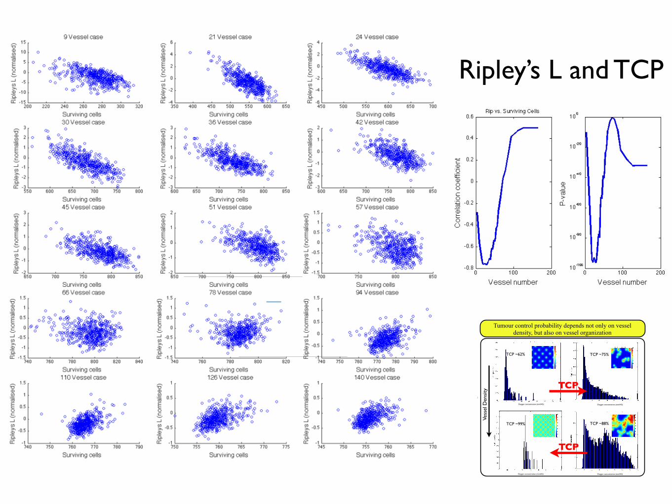
Ripley’s L and TCP
Towards patient-specific biology-driven heterogeneous radiation planning: using a computational model of tumor growth to identify
novel radiation sensitivity signatures.Jacob G Scott1,2, David Basanta1, Alex G Fletcher2, Philip K Maini2, Alexander RA Anderson1
1Integrated Mathematical Oncology, H. Lee Moffitt Cancer Center and Research Institute, Tampa, FL2Wolfson Centre for Mathematical Biology, Mathematical Institute, University of Oxford, Oxford, UK
Adapting radiotherapy to hypoxic tumours 4909
Figure 1. Pre- and post-contrast T1-weighted MR images taken in the coronal plane through thehead of the dog with a spontaneous sarcoma. The gross tumour volume (GTV) is enclosed by thewhite contour, while the tongue (T) and mandible (M) are indicated.
This is reflected in figure 2, showing a corresponding image of the tracer concentration inthe tumour. With respect to blood (and thus oxygen) supply, the tumour periphery mayqualitatively be characterized as normoxic, while the core is probably hypoxic or necrotic.
The tentative pO2 distribution (in frequency form) in the canine tumour, as obtained fromthe MR scaling procedure, is given in figure 3. In the same figure, the oxygen distributionobtained from Eppendorf histograph measurements (Brurberg et al 2005) is shown. The two
4910 E Malinen et al
Figure 2. Image of the concentration (in mM) of the contrast agent in the central coronal plane ofthe tumour.
Figure 3. Frequency histograms of the tumour oxygen tension in the canine patient, as determinedby the Eppendorf histograph (Brurberg et al 2005) and the MR analysis.
plots appear similar and rather log-normally distributed, but both have a high frequency ofreadings at the lowest oxygen level. The measured median and mean pO2 levels obtainedfrom the histograph were 8.5 and 13.9 mm Hg, respectively, against 13.6 and 16.6 mm Hg,respectively, estimated from the tentative MR analysis. The correlation coefficient betweenthe histograms was 0.88, and a rank sum test and a Kolmogorov–Smirnov test showed thatthe histograms were not significantly different (p values of 0.20 and 0.14, respectively). The‘hypoxic fraction’, i.e. the fraction of pO2 readings smaller than 5 mm Hg were 0.42 and0.28 for the histograph and MR analysis, respectively. For the current case, it is tentativelyassumed that the MR analysis provides pO2-related images that are biologically relevant.
The compartmental volumes and corresponding mean pO2 levels are given in table 1.In figure 4, coronal images displaying the tumour compartments are shown. It appears thatthe compartmental volumes vary considerably with the coronal plane position although thetumour periphery appears to have higher pO2 levels than the tumour core. As evident, thehypoxic compartments are not spatially continuous, but appear as multiple foci within thegross tumour volume. In figure 5, a 3D reconstruction of hence derived DICOM structure setsused in the treatment planning is displayed.
Biology and microenvironment affect radiation therapy efficacy
Macroscopic hypoxia correlates with radiocontrast uptake, and dose modulation is efficacious, in silico1
In this work, we use a proliferation-invasion-radiotherapy(PIRT) model [7] of GBM growth and response to therapy toaccount for patient-specific tumor proliferation and invasionkinetics combined with a multi-objective evolutionary algorithm(MOEA) for IMRT optimization [8] to demonstrate the potentialto improve tumor control while reducing dose to normal tissuerelative to the standard-of-care. Specifically, we applied themethodology presented in Holdsworth et al (2012) [8] with amore realistic set of optimization inputs, to a cohort of 11 GBMpatients, and compared patient-individualized, optimized IMRTplans with standard-of-care plans. Across this cohort of GBMpatients with diverse imaging patterns, we predicted the benefit ofthe patient-individualized, optimized plans in terms of normaltissue dose, therapeutic ratio and simulated treatment benefit.
Figure 1. Parameter generation for the patient-specific biomathematical model. 1. Determine radial measurements from serial T1Gd andT2/FLAIR magnetic resonance imaging. 2. Compute the invisibility index (D/r) from intra-study T1Gd and T2/FLAIR radial measurements. 3. Computethe radial velocity (2
!!!!!!!Dr
p) from serial T1Gd or T2/FLAIR radial measurements.
doi:10.1371/journal.pone.0079115.g001
Table 1. Optimization Restrictions.
Maximum Fraction/Dose Region
5 Gy Peak Fraction Inside T2/FLAIR
2.5 Gy Peak Fraction Outside T2/FLAIR
65 Gy Peak Dose Outside T2/FLAIR
0.4–1.4 Gy EUD* Fraction Outside T1Gd
*Patient-specific.doi:10.1371/journal.pone.0079115.t001
Patient-Specific Radiotherapy for Glioblastoma
PLOS ONE | www.plosone.org 2 November 2013 | Volume 8 | Issue 11 | e79115
•Radiation dose/fraction is known to depend heavily on local oxygen concentration as well as intrinsic cell parameters•Our ability to quantify these parameters in patients is maturing, but has not translated to the clinic
directly after the scans showed that the i.v.-injected Alexa 680-AC133 mAb had bound to almost all CSC marker-positive cellsin the tumor, verifying that the injected Alexa 680-AC133 mAbhad penetrated the tumor tissue efficiently (Fig. 3E, Left). Toidentify the CSCs ex vivo, the tumor single-cell suspensions werecostained with the AC141 antibody, which is specific for a secondstem cell-specific epitope of CD133. As expected, binding of theinjected Alexa 680-labeled isotype control antibody to CSCs couldnot be detected (Fig. 3E, Right).
FMT Imaging of Intracerebral Xenograft Tumors. Antibodies haveonly limited access to the brain because the undisturbed blood–brain barrier (BBB) is impermeable to macromolecules, andwhether systemically administered antibodies can reach extra-vascular targets in brain tumors with a disturbed BBB is of greatinterest (34, 35). We therefore wanted to find out whether theAC133 mAb is suitable for imaging orthotopically growingAC133+ glioma xenografts. We indeed could detect orthotopicallygrowing NCH421k gliomas noninvasively by NIR FMT imagingupon i.v. injection of the Alexa 680-labeled AC133 mAb (Fig. 3F,Upper Left), and the signal caused by the Alexa 680-AC133 mAb
also could be detected directly postmortem on the excised tu-mor-bearing brains (Fig. 3F, Lower Left).
PET Imaging of Tumor Stem Cell-Derived s.c. Xenografts. After theFMT studies had demonstrated that noninvasive mAb-mediatedvisualization of AC133+ CSCs was possible in principle, we ex-plored immuno-PET detection of AC133+ CSCs. The 64Cu-NOTA-AC133 mAb strongly marked s.c. growing NCH421k gliomas at 24and 48 h postinjection (p.i.) (Fig. 4A, Left and Center), despite theconsiderably lower expression of AC133 on NCH421k cells ascompared with CD133-overexpressing U251 cells (see Fig. 1A andFig. S3A). Particularly remarkable was the much higher tracer up-take liver [an organ exhibiting relatively high unspecific activitybecause of high blood perfusion, antibody metabolism, andpotential transchelation of 64Cu (28, 36)]. The tumor-to-con-tralateral background, tumor-to-blood pool, and tumor-to-livercontrasts were 21.4 ± 8.2, 2.7 ± 0.9, and 2.6 ± 0.8 at 24 h and32.8 ± 19, 6.4 ± 2.5, and 5.4 ± 1.8 at 48 h p.i., respectively. The64Cu-NOTA-isotype control antibody caused only a very weaktumor signal. As judged by visual inspection (Fig. 4A, Right) andaccording to in vivo and in vitro quantification (Fig. 4 B and C),
Fig. 2. PET/CT imaging and biodistribution of 64Cu-NOTA-AC133 mAb in mice bearing s.c. implanted U251 gliomas overexpressing CD133. Nude mice re-ceived !8.0 ± 0.5 MBq 64Cu-NOTA-AC133 mAb via tail vein injection, and PET/CT images were acquired. The mice carried AC133" U251 wild-type and AC133/CD133-overexpressing U251 gliomas in the left and right flanks, respectively. (A) Representative transverse tumor and coronal whole-body PET and fused PET/CT sections at 24 and 48 h p.i. (B) Uptake of 64Cu-NOTA-AC133 mAb as measured by microPET in various organs and AC133" and AC133-overexpressing tumorsat 24 and 48 h p.i. Values are the mean %IA/g of tissue. (C) Ex vivo biodistribution at 24 and 48 h p.i. Values are the mean %IA/g of tissue. n = 7–8 mice pergroup. ***P < 0.001, t test; values represent means ± SD.
Gaedicke et al. PNAS Early Edition | 3 of 10
MED
ICALSC
IENCE
SPN
ASPL
US
1. Malinen et al. Phys Med Biol 2006 2. Corwin et al. PLoS ONE 2013 3. Alfonso et al., PLoS ONE 2014 4. Leder et al, Cell 2014 5. Gaedicke et al., PNAS 2014. 6. Scott et al. PLoS Comp Biol 2014ACKNOWLEDGEMENT: This work sponsored in part by the Moffitt Cancer Center PSOC, NIH/NCI U54CA143970
XRT dose modulation using putative stem distribution3 and dynamics4 shown effective in silico and in vivo4
Cell diffusivity and replication can be inferred from MRI imaging, allowing for understanding of growth prediction and dose shape modification2
Non-invasive PET imaging reported with an anti-body to CD-1335 (putative stem marker)
Several layers of heterogeneity effect radiation efficacy
Figure W7. Segmentation of viable tissue. (A) Representative immunohistochemistry (IHC) staining of pimonidazole in orthotopicMDA-MB-231 tumors from mice given tap water or water containing sodium bicarbonate to drink. (B) Computational segmentationof viable (green) and nonviable (pink) tissues. (C) Positive pixel analysis of segmented viable tissue showing intensity of pimonidazolestaining: blue indicates negative staining, orange indicates moderate staining, and red indicates strong staining.
N
Quantitative Histologyyields vessel organization
Radiomicsyields vessel density
Microenvironmental feedback Lattice based CAStem hierarchy
Non stem-driven tumourhigh vessel density
Stem-driven tumour low vessel densityOxygen concentration (mmHG)
Oxygen concentration (mmHG)
Vess
el D
ensi
ty
TCP
TCP
Oxygen concentration (mmHG)
Oxygen concentration (mmHG)
Tumour control probability depends not only on vessel density, but also on vessel organization
Enabling translation - information from several scales
Optimized plan
Image credit: Unkelbach et a. doi: 10.1088/0031-9155/59/3/771
TCP ~62% TCP ~75%
TCP ~99% TCP ~88%
If I’m not around the poster and you want to chat, this is what I look like. Feel free to contact me at [email protected] or follow on twitter @CancerConnector. You can find this poster
on line here:
Mathematical model of a stem driven tumour in a heterogeneous vascular environment6
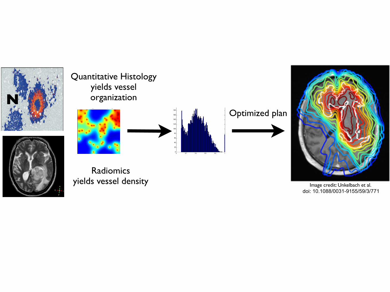
Towards patient-specific biology-driven heterogeneous radiation planning: using a computational model of tumor growth to identify
novel radiation sensitivity signatures.Jacob G Scott1,2, David Basanta1, Alex G Fletcher2, Philip K Maini2, Alexander RA Anderson1
1Integrated Mathematical Oncology, H. Lee Moffitt Cancer Center and Research Institute, Tampa, FL2Wolfson Centre for Mathematical Biology, Mathematical Institute, University of Oxford, Oxford, UK
Adapting radiotherapy to hypoxic tumours 4909
Figure 1. Pre- and post-contrast T1-weighted MR images taken in the coronal plane through thehead of the dog with a spontaneous sarcoma. The gross tumour volume (GTV) is enclosed by thewhite contour, while the tongue (T) and mandible (M) are indicated.
This is reflected in figure 2, showing a corresponding image of the tracer concentration inthe tumour. With respect to blood (and thus oxygen) supply, the tumour periphery mayqualitatively be characterized as normoxic, while the core is probably hypoxic or necrotic.
The tentative pO2 distribution (in frequency form) in the canine tumour, as obtained fromthe MR scaling procedure, is given in figure 3. In the same figure, the oxygen distributionobtained from Eppendorf histograph measurements (Brurberg et al 2005) is shown. The two
4910 E Malinen et al
Figure 2. Image of the concentration (in mM) of the contrast agent in the central coronal plane ofthe tumour.
Figure 3. Frequency histograms of the tumour oxygen tension in the canine patient, as determinedby the Eppendorf histograph (Brurberg et al 2005) and the MR analysis.
plots appear similar and rather log-normally distributed, but both have a high frequency ofreadings at the lowest oxygen level. The measured median and mean pO2 levels obtainedfrom the histograph were 8.5 and 13.9 mm Hg, respectively, against 13.6 and 16.6 mm Hg,respectively, estimated from the tentative MR analysis. The correlation coefficient betweenthe histograms was 0.88, and a rank sum test and a Kolmogorov–Smirnov test showed thatthe histograms were not significantly different (p values of 0.20 and 0.14, respectively). The‘hypoxic fraction’, i.e. the fraction of pO2 readings smaller than 5 mm Hg were 0.42 and0.28 for the histograph and MR analysis, respectively. For the current case, it is tentativelyassumed that the MR analysis provides pO2-related images that are biologically relevant.
The compartmental volumes and corresponding mean pO2 levels are given in table 1.In figure 4, coronal images displaying the tumour compartments are shown. It appears thatthe compartmental volumes vary considerably with the coronal plane position although thetumour periphery appears to have higher pO2 levels than the tumour core. As evident, thehypoxic compartments are not spatially continuous, but appear as multiple foci within thegross tumour volume. In figure 5, a 3D reconstruction of hence derived DICOM structure setsused in the treatment planning is displayed.
Biology and microenvironment affect radiation therapy efficacy
Macroscopic hypoxia correlates with radiocontrast uptake, and dose modulation is efficacious, in silico1
In this work, we use a proliferation-invasion-radiotherapy(PIRT) model [7] of GBM growth and response to therapy toaccount for patient-specific tumor proliferation and invasionkinetics combined with a multi-objective evolutionary algorithm(MOEA) for IMRT optimization [8] to demonstrate the potentialto improve tumor control while reducing dose to normal tissuerelative to the standard-of-care. Specifically, we applied themethodology presented in Holdsworth et al (2012) [8] with amore realistic set of optimization inputs, to a cohort of 11 GBMpatients, and compared patient-individualized, optimized IMRTplans with standard-of-care plans. Across this cohort of GBMpatients with diverse imaging patterns, we predicted the benefit ofthe patient-individualized, optimized plans in terms of normaltissue dose, therapeutic ratio and simulated treatment benefit.
Figure 1. Parameter generation for the patient-specific biomathematical model. 1. Determine radial measurements from serial T1Gd andT2/FLAIR magnetic resonance imaging. 2. Compute the invisibility index (D/r) from intra-study T1Gd and T2/FLAIR radial measurements. 3. Computethe radial velocity (2
!!!!!!!Dr
p) from serial T1Gd or T2/FLAIR radial measurements.
doi:10.1371/journal.pone.0079115.g001
Table 1. Optimization Restrictions.
Maximum Fraction/Dose Region
5 Gy Peak Fraction Inside T2/FLAIR
2.5 Gy Peak Fraction Outside T2/FLAIR
65 Gy Peak Dose Outside T2/FLAIR
0.4–1.4 Gy EUD* Fraction Outside T1Gd
*Patient-specific.doi:10.1371/journal.pone.0079115.t001
Patient-Specific Radiotherapy for Glioblastoma
PLOS ONE | www.plosone.org 2 November 2013 | Volume 8 | Issue 11 | e79115
•Radiation dose/fraction is known to depend heavily on local oxygen concentration as well as intrinsic cell parameters•Our ability to quantify these parameters in patients is maturing, but has not translated to the clinic
directly after the scans showed that the i.v.-injected Alexa 680-AC133 mAb had bound to almost all CSC marker-positive cellsin the tumor, verifying that the injected Alexa 680-AC133 mAbhad penetrated the tumor tissue efficiently (Fig. 3E, Left). Toidentify the CSCs ex vivo, the tumor single-cell suspensions werecostained with the AC141 antibody, which is specific for a secondstem cell-specific epitope of CD133. As expected, binding of theinjected Alexa 680-labeled isotype control antibody to CSCs couldnot be detected (Fig. 3E, Right).
FMT Imaging of Intracerebral Xenograft Tumors. Antibodies haveonly limited access to the brain because the undisturbed blood–brain barrier (BBB) is impermeable to macromolecules, andwhether systemically administered antibodies can reach extra-vascular targets in brain tumors with a disturbed BBB is of greatinterest (34, 35). We therefore wanted to find out whether theAC133 mAb is suitable for imaging orthotopically growingAC133+ glioma xenografts. We indeed could detect orthotopicallygrowing NCH421k gliomas noninvasively by NIR FMT imagingupon i.v. injection of the Alexa 680-labeled AC133 mAb (Fig. 3F,Upper Left), and the signal caused by the Alexa 680-AC133 mAb
also could be detected directly postmortem on the excised tu-mor-bearing brains (Fig. 3F, Lower Left).
PET Imaging of Tumor Stem Cell-Derived s.c. Xenografts. After theFMT studies had demonstrated that noninvasive mAb-mediatedvisualization of AC133+ CSCs was possible in principle, we ex-plored immuno-PET detection of AC133+ CSCs. The 64Cu-NOTA-AC133 mAb strongly marked s.c. growing NCH421k gliomas at 24and 48 h postinjection (p.i.) (Fig. 4A, Left and Center), despite theconsiderably lower expression of AC133 on NCH421k cells ascompared with CD133-overexpressing U251 cells (see Fig. 1A andFig. S3A). Particularly remarkable was the much higher tracer up-take liver [an organ exhibiting relatively high unspecific activitybecause of high blood perfusion, antibody metabolism, andpotential transchelation of 64Cu (28, 36)]. The tumor-to-con-tralateral background, tumor-to-blood pool, and tumor-to-livercontrasts were 21.4 ± 8.2, 2.7 ± 0.9, and 2.6 ± 0.8 at 24 h and32.8 ± 19, 6.4 ± 2.5, and 5.4 ± 1.8 at 48 h p.i., respectively. The64Cu-NOTA-isotype control antibody caused only a very weaktumor signal. As judged by visual inspection (Fig. 4A, Right) andaccording to in vivo and in vitro quantification (Fig. 4 B and C),
Fig. 2. PET/CT imaging and biodistribution of 64Cu-NOTA-AC133 mAb in mice bearing s.c. implanted U251 gliomas overexpressing CD133. Nude mice re-ceived !8.0 ± 0.5 MBq 64Cu-NOTA-AC133 mAb via tail vein injection, and PET/CT images were acquired. The mice carried AC133" U251 wild-type and AC133/CD133-overexpressing U251 gliomas in the left and right flanks, respectively. (A) Representative transverse tumor and coronal whole-body PET and fused PET/CT sections at 24 and 48 h p.i. (B) Uptake of 64Cu-NOTA-AC133 mAb as measured by microPET in various organs and AC133" and AC133-overexpressing tumorsat 24 and 48 h p.i. Values are the mean %IA/g of tissue. (C) Ex vivo biodistribution at 24 and 48 h p.i. Values are the mean %IA/g of tissue. n = 7–8 mice pergroup. ***P < 0.001, t test; values represent means ± SD.
Gaedicke et al. PNAS Early Edition | 3 of 10
MED
ICALSC
IENCE
SPN
ASPL
US
1. Malinen et al. Phys Med Biol 2006 2. Corwin et al. PLoS ONE 2013 3. Alfonso et al., PLoS ONE 2014 4. Leder et al, Cell 2014 5. Gaedicke et al., PNAS 2014. 6. Scott et al. PLoS Comp Biol 2014ACKNOWLEDGEMENT: This work sponsored in part by the Moffitt Cancer Center PSOC, NIH/NCI U54CA143970
XRT dose modulation using putative stem distribution3 and dynamics4 shown effective in silico and in vivo4
Cell diffusivity and replication can be inferred from MRI imaging, allowing for understanding of growth prediction and dose shape modification2
Non-invasive PET imaging reported with an anti-body to CD-1335 (putative stem marker)
Several layers of heterogeneity effect radiation efficacy
Figure W7. Segmentation of viable tissue. (A) Representative immunohistochemistry (IHC) staining of pimonidazole in orthotopicMDA-MB-231 tumors from mice given tap water or water containing sodium bicarbonate to drink. (B) Computational segmentationof viable (green) and nonviable (pink) tissues. (C) Positive pixel analysis of segmented viable tissue showing intensity of pimonidazolestaining: blue indicates negative staining, orange indicates moderate staining, and red indicates strong staining.
N
Quantitative Histologyyields vessel organization
Radiomicsyields vessel density
Microenvironmental feedback Lattice based CAStem hierarchy
Non stem-driven tumourhigh vessel density
Stem-driven tumour low vessel densityOxygen concentration (mmHG)
Oxygen concentration (mmHG)
Vess
el D
ensi
ty
TCP
TCP
Oxygen concentration (mmHG)
Oxygen concentration (mmHG)
Tumour control probability depends not only on vessel density, but also on vessel organization
Enabling translation - information from several scales
Optimized plan
Image credit: Unkelbach et al. doi: 10.1088/0031-9155/59/3/771
TCP ~62% TCP ~75%
TCP ~99% TCP ~88%
If I’m not around the poster and you want to chat, this is what I look like. Feel free to contact me at [email protected] or follow on twitter @CancerConnector. You can find this poster on line here: http://dx.doi.org/10.6084/m9.figshare.979442
Mathematical model of a stem driven tumour in a heterogeneous vascular environment6

1
Fig 6.
ReferencesWeinberg, R. A. (2007). The biology of cancer. New York: Garland Science. M. Lynch, R. Burger, D. Butcher, and W. Gabriel (1993). The mutational meltdown in asexual populations. J. Hered. 84:339-344.Moran, Patrick Alfred Pierce: The Statistical Processes of Evolutionary Theory. Oxford, Clarendon Press (1962).
Key Factors in the Metastatic Process: Insights from Population Genetics
Christopher McFarland1*, Jacob Scott2,3,*, David Basanta3, Alexander Anderson3, Leonid Mirny1
1Harvard-MIT Division of Health Science & Technology, 2H. Lee Moffitt Cancer and Research Center, 3Integrative Mathematical Oncology, *contributed equally to this work
Fig 1. Prevalence and significance of micrometastases are poorly understood. Most micrometastases never progress to macroscopic size. In this case, small colonies of breast endothelial cells are found in the lung of a non-metastatic breast cancer patient
Background:Metastasis is a highly lethal and poorly understood process that
accounts for the majority cancer deathsPatterns of metastatic spread are not explained by deterministic
explain these patternsWe develop a stochastic model at the genomic level and use
population genetics techniques to explore this phenomenon
Modeling Metastasis:
A tumor was grown in silico by creating a population of single cells that stochastically undergo mitosis and cell death. Cells can gain passenger and driver mutations during division which are passed to their offspring
Results: Effect of primary tumor on Pmet
Success of metastases increases with primary tumor size
Exploring the observed Heterogeneity in genotypes:
We found that Pmet varied considerably between cells from all 100 primary tumors (Left), but less so between cells within the same primary tumor (Right)
Tumors that took longer than the average time to reach 106 cells
Late primary tumors of equivalent size were less likely to metastasize
Clinical Applications:
Modification of the stromal factor could be useful in the mitigation of metastasisThis concept has been shown to be efficacious in the prevention of
Skeletal Related Events (SREs) for prostate and breast cancer metastasis and is the driving concept behind RTOG 0622, a trial of injectable 153Sm for the prevention of bony metastasesThis concept could be applied to other organs for the prevention of
metastases
Conclusions/Future Directions:
Using a genotype scale population genetics model of tumor evolution we have elucidated several factors necessary for successful metastasisFuture directions include testing these predictions against extant
genotype data from primary tumors and metastatic tumors as well as further defining the stromal interaction for different primary tumor types and for different stromas.
Fig 5.
Fig 8.
Fig 7.
Driver Mutation
Passenger Mutation
B(d,p)*
D(N)*
*
Fig. 2
An aliquot of 103 cells was taken from a primary tumor when it reached 5x10⁵ and 106 cells and were then allowed to deposit into a foreign stroma and observed
A stromal penalty s was applied only to driver mutations acquired in the primary tumor because their effects will not be as strong in the new stroma, passenger mutations are not affected by the change in microenvironmentWe then measured the number of secondary tumors that grew into
successful metastases from each aliquot and calculate a probability of metastasis (Pmet)
Fig 3.
NKNDsspdB pp
dd )()1()1(),(
Results: Effect of stromal factor on Pmet
Cells derived from the larger primary tumor succeeded in harsher microenvironmentsMetastatic success is highly dependent upon stromal backgroundThree regimes were observed in the parameter space as s varied, one in which
metastasis was impossible (green), one in which it was certain (yellow) and one in which only cells from certain primary tumor succeed (white)We further define a value, scritical, above which Pmet>50%
Fig 4.
Feature of Model Observed Phenomenon
Population size determined by fitness of cells
Larger Tumors more likely to metastasize
Cells can acquire passenger mutations that are slightly
deleterious
Many micrometastases never grown to macroscopic size
Cells with more mutations are less likely to metastasize
Stromal environment reduces efficacy of driver mutations
Certain stromal conditions prohibit metastasis
Metastasis continues to mutate and evolve
Metastases with same founding cell can have
different fates
Cells divide and acquire mutations on individual basis
Large heterogeneity in probability of metastasis
within primary tumor
No pre-defined growth rate
Late primary tumors less likely to metastasize than early tumors of equivalent
size
100 primary tumors were grown and scritical was calculated for each cell as the tumor grewMedian scritical (blue)
increases with primary tumor sizeThere is significant
heterogeneity of metastatic potential between the individual cells within the tumors as shown by the 5th and 95th percentiles (red) of scritical
Pmet decreases with total number of mutations
We derived a way to calculate Pmet
for every cell in the 100 primary tumors at equivalent sizes when inoculated into a foreign stroma of s = ¾ (not show)Pmet decreased with number of
mutationsThe vast majority of total mutations
are passenger mutations
Fig 6.
Integrative Mathematical Oncology
NIH 1 U54 CA143970-01S
~100 meters
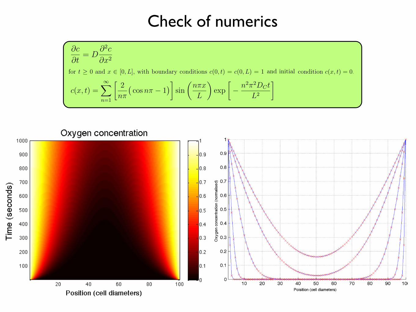
∂c
∂t= D
∂2c
∂x2(1.6)
for t ≥ 0 and x ∈ [0, L], with boundary conditions c(0, t) = c(0, L) = 1 and and initial
condition c(x, t) = 0.
We can solve this equation using separation of variables and solving for c = c + 1
which satisfies (1.6) and the boundary conditions c(0, t) = c(0, L) = 0 and initial condition
c(x, t) = −1. We find that the solution (see Appendix A) is given by
c(x, t) =∞
n=1
2
nπ
cosnπ − 1
sin
nπx
L
exp
− n2π2DCt
L2
. (1.7)
In Figure 1.8 we plot the oxygen concentation profile through the centre of a 100×100
domain which is devoid of cells at one-second intervals. The analytical solution (equation
(1.7)) is compared to the numerical solution of equation (1.5) at each lattice point for
time t = 1, 10, 100, 500 and 1, 000 seconds. We find excellent agreement between the two
solutions.
1.2.3.4 Time scales and updates
The difference in time scales that govern the diffusion of nutrients and that at which
cells operate is managed by updating the continuous part of the model many times per
cellular time step. This can become computationally expensive in this explicit scheme,
and therefore, we seek to minimize this number. However, for stability, we require that
the ∆tDc/∆x2term from equation (1.5) is less than 0.25 [56]. We therefore choose
∆tDc/∆x2= 0.1, which equates to updating oxygen every 0.25 seconds, or approximately
230, 400 times per cell cycle based on the parameters chosen (see Table 1.1). While we
assume the average cell cycle time to be τ = 16 hours, it is well known that cells in tissues
are not synchronized, and also that cell fate decisions such as apoptosis are made on
shorter time scales. To model this heterogeneity in division time and to more accurately
match the finer time scale associated with cell death due to microenvironmental cues
[68], we choose to update the HCA 100 times per cell cycle and scale the rates for
cell behaviour accordingly (reduced by a factor of 100), thereby reducing the oxygen
calculations to 2, 304 updates per HCA update.
15
Check of numerics
