eﬃcient use of 3d environment models for mobile robot ... · eﬃcient use of 3d environment...

Efficient Use of 3D Environment Models

for Mobile Robot

Simulation and Localization

Andreu Corominas Murtra, Eduard Trulls,Josep M. Mirats Tur, Alberto Sanfeliu

Institut de Robotica i Informatica IndustrialC/Llorens i Artigas 4-6. 08028. Barcelona. Spain

{acorominas,etrulls,jmirats,asanfeliu}@iri.upc.edu

http://www.iri.upc.edu

Abstract. This paper provides a detailed description of a set of algo-rithms to efficiently manipulate 3D geometric models to compute phys-ical constraints and range observation models, data that is usually re-quired in real-time mobile robotics or simulation. Our approach uses astandard file format to describe the environment and processes the modelusing the openGL library, a widely-used programming interface for 3Dscene manipulation. The paper also presents results on a test model forbenchmarking, and on a model of a real urban environment, where thealgorithms have been effectively used for real-time localization in a largeurban setting.

Keywords: 3D environment models, observation models, mobile robot,3D localization, simulation, openGL.

1 Introduction

For both simulation or real-time map-based localization, the mobile roboticscommunity needs to implement the computation of expected environment con-straints and expected sensor observations, the latter also called sensor models.For all these computations, an environment model is required and its fast andaccurate manipulation is a key point for successful results of upper-level appli-cations. This is even more important since current trends on mobile roboticsleads to 3D environment models, which are richer descriptions of the reality butharder models to process.

Using computer accelerated graphics card for fast manipulation of 3D sceneshas been addressed by robotic researchers from some yars ago, specially in thesimulation domain [4, 2, 1], but it remains less explored in real-time localization.In real-time particle filter localization [8, 3], expected environment constraintsand expected observations are computed massively at each iteration from eachparticle position, causing the software modules in charge of such computationsbeing a key piece for the final success of the whole system. Unlike simulation

2 Corominas Murtra, A. et al.

field, there exists few work reporting the use of accelerated graphics cards toimplement the online computation of expected observations [5].

Moreover, detailed descriptions on processing 3D geometric models to effi-ciently compute physical constraints or expected observations are not commonin the robotics literature. 3D geometric models have started to become an es-sential part of mobile robot environment models in recent years, specially forapplications targeting outdoor urban environments, and thanks in part to theavailability of powerful and affordable graphics cards on home computers. Thispaper wants to remedy the lack of a detailed description on how to efficientlymanipulate such models, presenting in a detailed way the algorithms for anoptimal use of the graphics card acceleration through the openGL library [7].Thanks to their fast computation, the presented algorithms are successfully usedfor real-time map-based localization in a large urban pedestrian environment,demonstrating the potential of our implementation.

The paper begins introducing the 3D environment model in section 2. Sec-tion 3 details the algorithms to compute the physical constraints of wheeledplatforms within the environment. Section 4 presents the algorithm to computeexpected range observations, minimizing the computation time while keepingsensor’s accuracy. Section 5 evaluates the performance of the algorithms andbriefly describes a real application example. Finally, section 6 concludes thework.

2 Overview of the 3D Environment Model

The goal of our environment model is to represent the 3D geometry of a real,urban pedestrian environment in a useful way for map-based localization andsimulation. Thus, the model incorporates the most static part of the environ-ment, such as buildings, floor, benchs, and other fixed urban furniture.

Our approach uses the .obj geometry definition file format [6]. Originallydeveloped for 3D computer animation, it has become an open format and a de

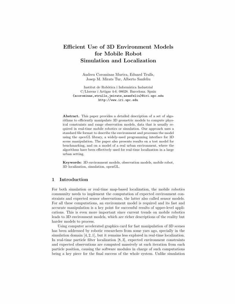
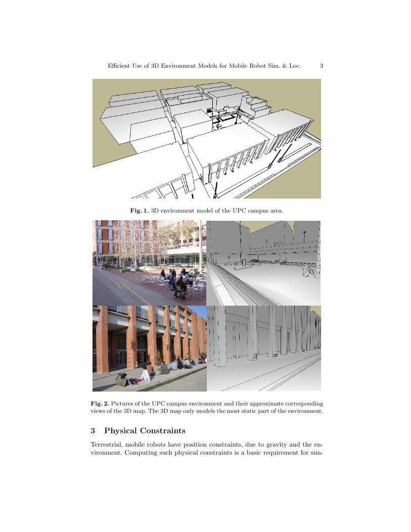
facto exchange standard. We use two different maps for our intended application.One map features the full environment, M, while the other consists only of thosesurfaces traversable by the robot, Mfloor, leaving holes instead of modellingobstacles. Figure 1 shows a view of the full model for the UPC (UniversitatPolitecnica de Catalunya) campus area and figure 2 shows real pictures of thisenvironment and their approximate corresponding views in the 3D model.

This environment model implicity defines a coordinate frame in which all thegeometry is referenced. Therefore a 3D position can be expressed with respectto the map frame as follows:

XMp = (xM

p , yMp , zM

p , θMp , φM

p , ψMp ) (1)

where the xyz coordinates define the location of the position and the θφψ co-ordinates parametrize the position attitude by means of the three Euler anglesheading, pitch and roll.

Efficient Use of 3D Environment Models for Mobile Robot Sim. & Loc. 3

Fig. 1. 3D environment model of the UPC campus area.

Fig. 2. Pictures of the UPC campus environment and their approximate correspondingviews of the 3D map. The 3D map only models the most static part of the environment.

3 Physical Constraints

Terrestrial, mobile robots have position constraints, due to gravity and the en-vironment. Computing such physical constraints is a basic requirement for sim-


ulation but also for map-based localization, since the search space is reduceddramatically, therefore improving the performance of the localization algorithm.

3.1 Gravity constraints

A wheeled robot will always lie on the floor, due to gravity. For relatively slowplatforms in can be assumed as well that the whole platform is a rigid body, sothat a suspension system, if present, does not modify the attitude of the vehicle.With these assumptions, gravity constraints for height, pitch and roll can bederived from the environment.

The height constraint sets a height, zM , for a given coordinate pair (xM , yM ).To compute it only the floor map is used. Algorithm 1 outlines the algorithm.The key idea is to renderize the 3D model from an overhead view point, settinga projection that limits the rendering volume in depth and aperture in orderto renderize only the relevant part of the model. Afterwards, by means of anopenGL routine, the algorithm reads the depth of the central pixel.

Algorithm 1 Height constraint algorithm for 3D models

INPUT: Mfloor, (xM , yM )

OUTPUT: gz

setWindowSize(5, 5); //sets rendering window size to 5x5 pixelssetProjection(1◦, 1, zmin, zmax) //1◦ of aperture, aspect ratio, depth limitsXoverhead = (xM , yM , zM

overhead, 0, π/2, 0); //sets an overhead view point, pitch= π/2renderUpdate(Mfloor, Xoverhead); //renders the model from Xoverhead

r = readZbuffer(3, 3); //reads depth of central pixelgz = zM

overhead − r;return gz;

The pitch constraint fixes the pitch variable of the platform to a given coor-dinate triplet (xM

p , yMp , θM

p ). The algorithm to compute the pitch constraint isoutlined in algorithm 2. It employs the previous height constraint algorithm tocompute the floor model’s difference in height between the platform’s frontmostand backmost points, gzf and gzb. The pitch angle is then computed using triv-ial trigonometry, while L is the distance between the above mentioned platformpoints. The roll constraint can be found in a similar way but computing theheight constraint for the leftmost and rightmost platform points. Please notethat the roll constraint applies to all wheeled platforms, but the pitch constraintdoes not apply to two-wheeled, self-balancing robots, such as ours, based onSegway platforms.

3.2 Offline height map computation

The constraints presented in the previous section are computed intensively infiltering applications such as map-based localization. To speed up online compu-tations during real-time execution, a height grid is computed offline for the floor


Algorithm 2 Pitch constraint algorithm for 3D models

INPUT: Mfloor, L, (xMp , yM

p , θMp )

OUTPUT: gφ

xMf = xM

p + L2

cos θMp ; //compute the platform’s frontmost point

yMf = yM

p + L2

sin θMp ; //likewise

gzf = heightConstraint(xMf , yM

f ); //compute height at frontmost pointxM

b = xMp −

L2

cos θMp ; //compute the platform’s backmost point

yMb = yM

p −L2

sin θMp ; //likewise

gzb = heightConstraint(xMb , yM

b ); //compute height at backmost pointgφ = atan2(gzf − gzb, L);return gφ;

map. Gheight is then a grid containing the height value zM for pairs (xM , yM ),thus being a discrete representation of the height constraint with a xy step γ:

Gheight(i, j) = gz(xMp , yM

p ) | i = (int)xM

p − xM0

γ, j = (int)

yMp − yM

0

γ, (2)

where xM0

and yM0

are the map origin xy coordinates. The zM value is computedoffline by means of the height constraint (algorithm 1) along the grid points.Figure 3 shows the height grid for the UPC campus environment.

Note that this approach is valid for maps with a single traversable z-level,such as ours, and while our algorithms can be directly applied to multi-levelmaps further work would be required in determining the appropiate map sectionto compute. Since computing the pitch and roll constraints requires several zM

computations, the height grid speeds up these procedures as well. To avoid dis-cretization problems, specially when computing pitch and roll constraints usingGheight, we use lineal interpolation on the grid. Algorithm 3 summarizes the gridversion of the height constraint.

Algorithm 3 Grid version of the height constraint

INPUT: Gheight, (xMp , yM

p )OUTPUT: gz

i = (int)xM

p −xM0

γ; j = (int)

yMp −yM

0

γ

z1 = Gheight(i, j);(i2, j2) = nearestDiagonalGridIndex(); //i2 = i ± 1; j2 = j ± 1;z2 = Gheight(i2, j); //height of a neighbour cellz3 = Gheight(i, j2); //height of a neighbour cellz4 = Gheight(i2, j2); //height of a neighbour cellgz = interpolation(z1, z2, z3, z4, x

Mp , yM

p );return gz;


Fig. 3. Height grid, Gheight, of the UPC campus environment.

4 Range Observation Model

Another key factor in dealing with environment models is the computation ofexpected observations, also called sensor models, or simulated sensors. This isalso useful for both simulation and real-time map-based localization. This sectionoutlines how, from a given 3D position in the environment, expected 2D rangescans and expected 3D point clouds are computed. A common problem in eithercase is the computation of range data given the sensor position and a set of sensorparameters like angular aperture, number of points and angular accuracy. Tocompute these observation models, we use again openGL renderization and depthbuffer reading, but the approach specially focuses on minimizing the computationtime without violating sensor’s accuracy and resolution. This minimization isachieved by reducing the rendering window size and the renderig volume asmuch as possible, while keeping the sensor accuracy.

The goal of a range observation model is to find a matrix R of ranges fora given sensor position XM

s . Each element rij of the matrix R is the rangecomputation following the ray given by the angles αi and βj . Figure 4 shows

these variables as well as coordinate frames for the map, (XYZ)M

, and for thesensor, (XYZ)

s.

The range observation model has the following inputs:


Fig. 4. Model frame, sensor frame, angles αi and βj , and the output ranges rij .

– A 3D geometric model, M.– A set of sensor parameters: horizontal and vertical angular apertures, ∆α

and ∆β , horizontal and vertical angular accuracies, δα and δβ, the size ofthe range matrix, nα × nβ , and range limits, rmin, rmax.

– A sensor position, XMs = (xM

s , yMs , zM

s , θMs , φM

s , ψMs ).

The operations to execute in order to compute ranges rij are:

1. Set the projection to view the scene.2. Set the rendering window size.3. Render the scene from XM

s .4. Read the depth buffer of the graphics card and compute ranges rij .

Set the Projection. Before using the openGL rendering, the projection parame-ters have to be set. These parameters are the vertical aperture of the scene view,which is directly the vertical aperture of the modelled sensor, ∆β , an image as-pect ratio ρ, and two parameters limiting the viewing volume with two planesplaced at zN (near plane) and zF (far plane)1. These two last parameters coin-cide respectively with rmin and rmax of the modelled sensor. The only parameterto be computed at this step is the aspect ratio ρ. To do this, first the metricdimensions of the image plane, width, w, and height, h, have to be found. Theaspect ratio will be derived from them:

w = 2rmintg(∆α

2);h = 2rmintg(

∆β

2); ρ =

w

h; (3)

Figure 5 depicts the horizontal cross section of the projection with the associatedparameters. The vertical cross section is analogous to the horizontal one.

1 zN and zF are openGL depth values defined in the screen space.


Fig. 5. Horizontal cross section of the projection with the involved parameters. Greensquares represent the pixels at the image plane.

Set the rendering window size. Before rendering a 3D scene, the size of theimage has to be set. Choosing a size as small as possible is a key issue to speedup the proposed algorithm. Since range sensors have limited angular accuracy,we use that to limit the size of image, in order to avoid renderizing more pixelsthan those required. Given a sensor with angular accuracies δα and δβ , pixeldimensions of the rendering window are to:

pα = (int)2tg(∆α/2)

tg(δα); pβ = (int)2

tg(∆β/2)

tg(δβ); (4)

Figure 5 shows an horizontal cross section of the projection and the relatedvariables to compute the horizontal pixel size of the rendering window (thevertical pixel size is found analogously).

Render the scene. The scene is renderized from the view point situated at sensorpositionXM

s . Beyond computing the color for each pixel of the rendering window,the graphics card also associates to each one a depth value. Moreover, graphicscard are optimized to discard parts of the model escaping from the scene, thushaving limited the rendering window size and volume speeds up the renderingstep. Renderization can be execute in a hidden window.

Read the depth buffer. Depth values of each pixel are stored in the depth buffer

of the graphics card. They can be read by means of an openGL function thatreturns data in a matrix B of size pα×pβ , which is greater in size than the desiredmatrix R. Read depth values, bkl, are a normalized version of the renderizeddepth for each pixel. To obtain the desired ranges, we first have to compute theD matrix, which holds the non-normalized depth values, that is the depth value


of the pixels following the Xs direction:

k = (int)(1

2−

tg(αi)

2tg(∆α

2))pα; l = (int)(

1

2−

tg(βj)

2tg(∆β

2))pβ

dij =rminrmax

(rmax − bkl)(rmax − rmin);

(5)

The last equation undoes the normalization computed by the graphics card tostore the depth values. The D matrix has nα × nβ size, since we compute dij

only for the pixels of interest. Finally, with basic trigonometry we can calculatethe desired rij as:

rij =dij

cos(αi)cos(βj)(6)

Figure 6 shows the variables involved on this last step, showing the meaningof the dij and rij distances in an horizontal cross section of the scene. Equation 6presents numerical problems when αi or βj get close to π/2. This will limit theaperture of our sensor model. However, section 5 explains how to overcome thislimitation when modeling a real sensor with a wide aperture.

Fig. 6. Horizontal cross section of the projection, with distance dij and range rij ofthe corresponding klth pixel.

The overall procedure is outlined in algorithm 4. Inside the for loops, vari-ables k and l are directly functions of i and j respectively, so we can precomputeexpressions in equation 5 for k and l, and store values in a vector.

5 Experimental Evaluation

This section presents some results that evaluate the performance of our algo-rithms. Two range models are presented, corresponding to real laser scanners,


Algorithm 4 Range Sensor Model

INPUT: M, ∆α, ∆β, δα, δβ, nα, nβ , rmax, rmin, XMs

OUTPUT: R

w = 2rmintg(∆α

2); h = 2rmintg(

∆β

2); ρ = w

h;

glSetProjection(∆β, ρ, rmin, rmax);//rendering volume: vertical aperture, aspect ra-tio, depth limits

pα = (int)2 tg(∆α/2)tg(δα)

; pβ = (int)2tg(∆β/2)

tg(δβ);

glSetWindowSize(0, 0, pα, pβ);glRenderUpdate(M,XM

s ); //renders the model from the sensor positionB = glReadZbuffer(ALL IMAGE); //reads normalized depth valuesfor i = 1..nα do

αi = ∆α(0.5 −i

nα);

k = (int)(0.5 −tg(αi)

2tg(∆α/2))pα;

for j = 1..nβ do

βj = ∆β(0.5 −j

nβ);

l = (int)(0.5 −tg(βj)

2tg(∆β/2))pβ;

dij = rminrmax

(rmax−bkl)(rmax−rmin);

rij =dij

cos(αi)cos(φj);

end for

end for

return R;

and computational time is provided for a testbench 3D scene. Finally, we brieflydescribe the successful use of all presented algorithms for real-time map-basedlocalization.

5.1 Laser scanner models

Two kind of laser scanner models has been used, using the same software. Table 1summarizes the input parameters of these laser scanner models. Our implemen-tation sets angular accuracies equal to angular resolutions. Please note also that,due to application requirements, we only model part of the scan provided by theHokuyo laser.

Table 1. Input parameters of the laser scanner models

Input Parameter Leuze RS4 Hokuyo UTM 30-LX (partial)

∆α, ∆β 190◦, 1◦ 60◦, 1◦

nα, nβ 133, 5 points 241, 5 points

δα = ∆α/nα, δβ = ∆β/nβ 1.43◦, 0.2◦ 0.25◦, 0.2◦

rmin, rmax 0.3, 20 m 0.3, 20 m

Table 2 outlines the derived parameters of the models. Leuze device hasan horizontal aperture greater than 180◦ and that poses numerical problems on


Fig. 7. Time performance versus scene complexity for the Leuze RS4 laser scanner.The sphere object has m2 elements.

computing equation 6. This issue is overcome by dividing the computation in twoscanning sectors, each one with the half of sensor’s aperture, so the parametersgiven in table 2 in the Leuze column are for a single scanning sector.

Table 2. Derived parameters of the laser scanner models

Derived Parameter Leuze RS4 (per scanning sector) Hokuyo UTM 30-LX (partial)

w 0.655 m 0.346 m

h 0.005 m 0.005 m

ρ 125 66

pα 88 pixels 265 pixels

pβ 5 pixels 5 pixels

To evaluate the computational perfomance of the proposed implementationwhile increasing the scene complexity, we have done a set of experiments consist-ing on computing 100 times the Leuze model against a testbench environmentcomposed of a single sphere, while increasing the number of sectors and slicesof that shape. The results are shown in figure 7. For a given m, the sphere isformed by m sectors and m slices, and thus the scene has m2 elements.

Please note that using the same software implementation, other range mod-els of devices providing point clouds such as time-of-flight cameras or 3D laserscanners can be easily configured and computed.


5.2 Map-based localization

Gravity constraints and laser scanner models have been used for 3D, real-time,map-based localization of a mobile platform while it navigates autonomously onthe UPC campus area introduced in section 2. The mobile platform is a two-wheeled self-balancing Segway RMP200, equiped with two laser devices scanningover the horizontal plane forward and backward (Leuze RS4), and a third laserdevice (Hokuyo UTM 30-LX) scanning the vertical plane in front of the robot.A particle filter integrates data from these three scanners and from the platformencoders and inclinometers to output a position estimate. At each iteration ofthe filter, for each particle, height and roll constraints are calculated at thepropagation phase by means of the grid versions of gravity constraints, so anegligible time is spent during online executions. On the other hand, expectedrange observations are computed online using algorithm 4. The filter runs ona DELL XPS-1313 laptop at 5 Hz, using 50 particles. This implies that thecomputer was calculating 5×50×(133+133+241) rays per second. The approachhas been proved successful as will be documented in future publications.

6 Conclusions

Although efficient computation of 3D range observation models is commonplacein robotics for a wide range of applications, little effort has been put on doc-umenting algorithms to solve this issue. This paper details a set of algorithmsfor fast computation of range data from 3D geometric models of a given envi-ronment using the very well-known openGL programming library. Additionally,we show that the same principles can be applied to the computation of physicalconstraints of terrestrial mobile platforms and demonstrate our approach for acomputationally expensive, real-time application.

References

1. Friedmann, M., Petersen, K., von Stryk, O.: Simulation of Multi-Robot Teams withFlexible Level of Detail. In: Carpin, S., Noda, I., Pagello, E., Reggiani, M., vonStryk, O. (eds.) SIMPAR 2008. LNAI, vol. 5325. 2008.

2. Laue, T., Spiess, K., Rfer, T.: SimRobot - A General Physical Robot Simulator andIts Application in RoboCup. In: A. Bredenfeld, A. Jacoff, I. Noda, Y. Takahashi(Eds.), RoboCup 2005: Robot Soccer World Cup IX, LNAI, No. 4020. 2006.

3. Levinson, J., Montemerlo, M., Thrun, S.:Map-Based Precision Vehicle Localizationin Urban Environments. In: Proceedings of the Robotics: Science and Systems Con-ference. Atlanta, USA. June, 2007.

4. Michel, O.: Cyberbotics Ltd - WebotsTM: Professional Mobile Robot Simulation,In: International Journal of Advanced Robotic Systems, Vol. 1, Num. 1. 2004.

5. Nuske, S., Roberts, J., Wyeth, G.:Robust Outdoor Visual Localization Using aThree-Dimensional-Edge Map. In: Journal of Field Robotics, Num. 26, Vol. 9. 2009.

6. OBJ file format, http://local.wasp.uwa.edu.au/~pbourke/dataformats/obj/7. OpenGL, http://www.opengl.org8. Thrun, S., Fox, D., Burgard, W., Dellaert, F.:Robust Monte Carlo localization for

mobile robots. In: Artificial Intelligence, vol. 128. 2001.

eﬃcient use of 3d environment models for mobile robot ... · eﬃcient use of 3d environment...

Documents