eï¬ƒcient motion planning and control for underwater gliders

Efficient Motion Planning and Control for Underwater Gliders

Nina Mahmoudian

Dissertation submitted to the Faculty of theVirginia Polytechnic Institute and State University

in partial fulfillment of the requirements for the degree of

Doctor of Philosophyin

Aerospace Engineering

Craig A. Woolsey, ChairChristopher D. Hall

Wayne NeuDaniel J. Stilwell

September 8, 2009Blacksburg, Virginia

Keywords: Motion Control, Path Planning, Underwater GlidersCopyright 2009, Nina Mahmoudian

Efficient Motion Planning and Control for Underwater Gliders

Nina Mahmoudian

(ABSTRACT)

Underwater gliders are highly efficient, winged autonomous underwater vehicles thatpropel themselves by modifying their buoyancy and their center of mass. The center of massis controlled by a set of servo-actuators which move one or more internal masses relative to thevehicle’s frame. Underwater gliders are so efficient because they spend most of their time instable, steady motion, expending control energy only when changing their equilibrium state.Motion control thus reduces to varying the parameters (buoyancy and center of mass) thataffect the state of steady motion. These parameters are conventionally controlled throughfeedback, in response to measured errors in the state of motion, but one may also incorporatea feedforward component to speed convergence and improve performance.

In this dissertation, first an approximate analytical expression for steady turning motionis derived by applying regular perturbation theory to a realistic vehicle model to developa better understanding of underwater glider maneuverability, particularly with regard toturning motions. The analytical result, though approximate, is quite valuable because itgives better insight into the effect of parameters on vehicle motion and stability.

Using these steady turn solutions, including the special case of wings level glides, onemay construct feasible paths for the gliders to follow. Because the turning motion resultsare only approximate, however, and to compensate for model and environmental uncertainty,one must incorporate feedback to ensure convergent path following. This dissertation de-scribes the development and numerical implementation of a feedforward/feedback motioncontrol system intended to enhance locomotive efficiency by reducing the energy expendedfor guidance and control. It also presents analysis of the designed control system using slowlyvarying systems theory. The results provide (conservative) bounds on the rate at which thereference command (the desired state of motion) may be varied while still guaranteeing sta-bility of the closed-loop system. Since the motion control system more effectively achievesand maintains steady motions, it is intrinsically efficient.

The proposed control system enables speed, flight path angle, and turn rate, providing amechanism for path following. The next step is to implement a guidance strategy, togetherwith a path planning strategy, and one which continues to exploit the natural efficiency ofthis class of vehicle. The structure of the approximate solution for steady turning motionis such that, to first order in the turn rate, the glider’s horizontal component of motionmatches that of “Dubins’ car,” a kinematic car with bounded turn rates. Dubins’ car is aclassic example in the study of time-optimal control for mobile robots. For an underwaterglider, one can relate time optimality to energy optimality. Specifically, for an underwaterglider travelling at a constant speed and maximum flight efficiency (i.e., maximum lift-to-drag ratio), minimum time paths are minimum energy paths. Hence, energy-efficient pathscan be obtained by generating sequences of steady wings-level and turning motions. Theseefficient paths can, in turn, be followed using the motion control system developed in thiswork.

That this work received support from the Office of Naval Research under grant numberN00014-08-1-0012.

Acknowledgments

I am deeply indebted to my advisor, Craig Woolsey, for the incomparable opportunity that heprovided me. I am grateful for his encouraging guidance, his close attention to my research,his mentorship, and his extraordinary kindness. I aspire to achieve his level of academicscholarship and leadership.

I sincerely thank Dr. Mehdi Ahmadian for his enlightening comments and vision. Becauseof his encouragement and advice, I applied to Virginia Tech and started working with Dr.Craig Woolsey at the Department of Aerospace and Ocean Engineering, which had alwaysbeen my prime interest. I deeply appreciate his influence on the change of direction in thepath of my life.

I would like to thank the members of my committee, Christopher Hall, Daniel Stilwell,and Wayne Neu, for reviewing my dissertation and providing me with their comments, whichgreatly helped me to improve the quality of this dissertation.

My department is a happy home that I will truly miss. For their contributions to myprofessional preparation, I thank faculty members Dr. Leigh McCue and Dr. ChristopherHall. I also thank the administrative staff, Wanda Foushee, Janet Murphy, and RachelHall Smith, for their organizational prowess and friendship. A special thanks goes to SteveEdwards for all his help and support whenever I needed it.

Membership in the Nonlinear Systems Lab provided me with collaborators, colleagues,and friends for life. I thank Laszlo Techy, Bob Kraus, and Chris Cotting. I also thankpast lab members for their contributions and camaraderie, including Konda Reddy, AmandaYoung, and Enric Xagary.

Studying with my wonderful husband Mohammad made my journey at Virginia Tech anexceptionally unique experience. Taking classes together, discussing our research, preparingfor presentations, and planning for the future have never been more pleasant. His devotionand dedication will continue to take us to the higher heights.

I want to thank my family for their continuous support and encouragement. My brothersMani and Rasa’s affection have always been a great comfort. I also thank my parents, Naziand Taher; their love and caring go beyond what I have ever seen. I now fully appreciatethe emphasis my father has always put on ethics and values and feel overwhelmed when Iremember how my mother taught me to live, learn, and love. Who I have become, what Ibelieve in, and my ability to look towards a wonderful future are all because of her, and Iwish to dedicate this dissertation to her.

iii

Contents

Acknowledgments iii

Table of Contents iv

List of Figures vi

1 Introduction 1

2 Modeling 112.1 Vehicle Dynamic Model with Rectilinear Actuator Dynamics . . . . . . . . 11

2.1.1 Simplified Vehicle Dynamic Model with Rectilinear Actuator Dynamics 202.1.2 Vehicle Dynamic Model with Fixed Actuators . . . . . . . . . . . . . 23

2.2 Vehicle Dynamic Model with Cylindrical Actuator Dynamics . . . . . . . . . 25

3 Steady Motion 313.1 Wings Level Gliding Flight . . . . . . . . . . . . . . . . . . . . . . . . . . . . 323.2 Steady Turning Flight . . . . . . . . . . . . . . . . . . . . . . . . . . . . . . 34

3.2.1 Turning Flight for Aircraft . . . . . . . . . . . . . . . . . . . . . . . . 353.2.2 Turning Flight for Underwater Gliders . . . . . . . . . . . . . . . . . 37

3.3 Numerical Case Study: Slocum . . . . . . . . . . . . . . . . . . . . . . . . . 43

4 Motion Control 504.1 Feedforward/Feedback Controller Design . . . . . . . . . . . . . . . . . . . . 534.2 Flight Path Control . . . . . . . . . . . . . . . . . . . . . . . . . . . . . . . . 574.3 Turn Rate Control . . . . . . . . . . . . . . . . . . . . . . . . . . . . . . . . 584.4 Stability Analysis of Closed-Loop System . . . . . . . . . . . . . . . . . . . . 594.5 Simulation Results . . . . . . . . . . . . . . . . . . . . . . . . . . . . . . . . 62

5 An Illustrative Example 695.1 Problem Definition . . . . . . . . . . . . . . . . . . . . . . . . . . . . . . . . 705.2 Stability Near Hyperbolic Equilibria . . . . . . . . . . . . . . . . . . . . . . . 715.3 Feedforward/Feedback Controller Design . . . . . . . . . . . . . . . . . . . . 755.4 Stability Analysis of Closed-Loop System . . . . . . . . . . . . . . . . . . . . 775.5 Simulation Results . . . . . . . . . . . . . . . . . . . . . . . . . . . . . . . . 79

iv

CONTENTS v

6 Guidance 856.1 Path Planning . . . . . . . . . . . . . . . . . . . . . . . . . . . . . . . . . . . 86

6.1.1 Dubins’ Car . . . . . . . . . . . . . . . . . . . . . . . . . . . . . . . . 876.1.2 Dubins’ Car with Control Rate Limits . . . . . . . . . . . . . . . . . 896.1.3 Dubins’ Car in the Presence of Currents . . . . . . . . . . . . . . . . 91

6.2 Guidance Strategies . . . . . . . . . . . . . . . . . . . . . . . . . . . . . . . . 926.2.1 Planar Trajectory Tracking . . . . . . . . . . . . . . . . . . . . . . . 926.2.2 Coordination on Helical Paths . . . . . . . . . . . . . . . . . . . . . . 94

6.3 Simulation Results . . . . . . . . . . . . . . . . . . . . . . . . . . . . . . . . 95

7 Conclusions and Future Work 102

Bibliography 104

List of Figures

1.1 The underwater glider Slocum solid model [1]. . . . . . . . . . . . . . . . . . 21.2 The blended wing-body underwater glider Liberdade/XRay solid model [1]. . 7

2.1 Illustration of point mass actuators. . . . . . . . . . . . . . . . . . . . . . . . 122.2 Illustration of the aerodynamic angles. . . . . . . . . . . . . . . . . . . . . . 172.3 Rotational transformations between various reference frames. (Adapted from

[2].) . . . . . . . . . . . . . . . . . . . . . . . . . . . . . . . . . . . . . . . . 182.4 Reference frames. . . . . . . . . . . . . . . . . . . . . . . . . . . . . . . . . . 232.5 Illustration of point mass actuators. . . . . . . . . . . . . . . . . . . . . . . . 262.6 Illustration of point mass actuators. . . . . . . . . . . . . . . . . . . . . . . . 27

3.1 The underwater glider Slocum. (Solid model in Rhinoceros 3.0.) . . . . . . . 443.2 Wings level equilibrium glide characteristics for Slocum model. . . . . . . . . 443.3 Wings level (ε = 0) and turning (ε = 0.01) flight paths for the Slocum model. 463.4 Eigenvalue plots for actual and approximate equilibria for 0 < ε < 0.1. (A

closer view of the dominant eigenvalues is shown at the right.) . . . . . . . . 46

4.1 A steady motion-based feedforward/feedback control system. . . . . . . . . . 514.2 Lateral moving mass location (open- and closed-loop). . . . . . . . . . . . . . 634.3 Slocum path in response to command sequence. . . . . . . . . . . . . . . . . 644.4 Glide path angle response to command sequence. . . . . . . . . . . . . . . . 654.5 Turn rate response to command sequence. . . . . . . . . . . . . . . . . . . . 664.6 Variation in longitudinal moving mass position from nominal. . . . . . . . . 674.7 Lateral moving mass position and turn rate. . . . . . . . . . . . . . . . . . . 674.8 Longitudinal moving mass position and flight path angle. . . . . . . . . . . . 684.9 Slocum path in response to feedback and feedforward/feedback compensator. 68

5.1 True and approximate equilibrium parameterized by ε. . . . . . . . . . . . . 715.2 True and approximate eigenvalues parameterized by 0 < ε < 1. . . . . . . . 725.3 True and approximate eigenvalues parameterized by 0 < ε ≤ 0.1. . . . . . . 755.4 Control loop. . . . . . . . . . . . . . . . . . . . . . . . . . . . . . . . . . . . 765.5 Open-loop response to step input. . . . . . . . . . . . . . . . . . . . . . . . . 815.6 Closed-loop response to step input. . . . . . . . . . . . . . . . . . . . . . . . 815.7 Tracking response of the system τ = 1 and xd = 1.1. . . . . . . . . . . . . . . 825.8 Tracking response of the system τ = 1, and xd = 1.4. . . . . . . . . . . . . . 835.9 Tracking response of the system τ = 10, and xd = 1.4. . . . . . . . . . . . . . 83

vi

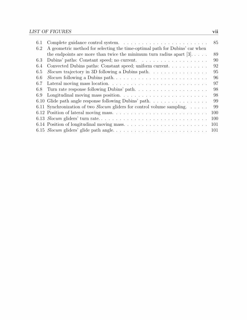
LIST OF FIGURES vii

6.1 Complete guidance control system. . . . . . . . . . . . . . . . . . . . . . . . 856.2 A geometric method for selecting the time-optimal path for Dubins’ car when

the endpoints are more than twice the minimum turn radius apart [3]. . . . . 896.3 Dubins’ paths: Constant speed; no current. . . . . . . . . . . . . . . . . . . 906.4 Convected Dubins paths: Constant speed; uniform current. . . . . . . . . . . 926.5 Slocum trajectory in 3D following a Dubins path. . . . . . . . . . . . . . . . 956.6 Slocum following a Dubins path. . . . . . . . . . . . . . . . . . . . . . . . . . 966.7 Lateral moving mass location. . . . . . . . . . . . . . . . . . . . . . . . . . . 976.8 Turn rate response following Dubins’ path. . . . . . . . . . . . . . . . . . . . 986.9 Longitudinal moving mass position. . . . . . . . . . . . . . . . . . . . . . . . 986.10 Glide path angle response following Dubins’ path. . . . . . . . . . . . . . . . 996.11 Synchronization of two Slocum gliders for control volume sampling. . . . . . 996.12 Position of lateral moving mass. . . . . . . . . . . . . . . . . . . . . . . . . . 1006.13 Slocum gliders’ turn rate. . . . . . . . . . . . . . . . . . . . . . . . . . . . . . 1006.14 Position of longitudinal moving mass. . . . . . . . . . . . . . . . . . . . . . . 1016.15 Slocum gliders’ glide path angle. . . . . . . . . . . . . . . . . . . . . . . . . . 101

List of Tables

1.1 Specifications of “Legacy gliders” [4]. . . . . . . . . . . . . . . . . . . . . . . 41.2 Specifications of other underwater gliders [4]. . . . . . . . . . . . . . . . . . . 6

2.1 Generalized inertia matrix. . . . . . . . . . . . . . . . . . . . . . . . . . . . . 142.2 Generalized velocity and momentum. . . . . . . . . . . . . . . . . . . . . . . 152.3 Generalized velocity and momentum. . . . . . . . . . . . . . . . . . . . . . . 282.4 Moving mass generalized inertia matrix. . . . . . . . . . . . . . . . . . . . . 292.5 Generalized inertia matrix. . . . . . . . . . . . . . . . . . . . . . . . . . . . . 30

3.1 Approximate and actual steady motion conditions for V0 = 1.5 knots and α=4.3◦. . . . . . . . . . . . . . . . . . . . . . . . . . . . . . . . . . . . . . . . . 48

3.2 Approximate and actual steady motion conditions for V0 = 2.0 knots and α=4.3◦. . . . . . . . . . . . . . . . . . . . . . . . . . . . . . . . . . . . . . . . . 49

3.3 Approximate and actual steady motion conditions for V0 = 1 knot and α= 4.3◦. 49

viii

Chapter 1

Introduction

The ocean covers approximately 71 percent of the surface of Earth. Ocean water has a great

impact on the climate of Earth; however, many global oceanographic phenomena are not yet

well understood [5]. Research efforts are focused on developing models and tools to better

understand the coupled physical and biological dynamics of the oceans and their impact on

the environment, from marine ecosystems to the global climate [6].

The main challenge is collecting data “in a vast, inhospitable, and unforgiving” ocean

environment [7]. Different sensing methods are being used to measure pressure, tempera-

ture, salinity, sound speed, density, and velocity in the ocean [7]. Surface drifters and deep

ocean floats are examples of traditional measurement systems [7]. The use of remote sensing

techniques (acoustic and electromagnetic) from satellites in recent years helped a lot of the

ocean surface studies [7], but limited measurements under ocean surface can be made with

traditional methods. In recent years, marine scientists have used autonomous underwater

vehicles (AUVs) as an important tool in gathering oceanographic data, replacing the tradi-

tional process of using expendable sensors, moored profilers, and floats in deep ocean. AUVs

are able to operate at a fraction of overall costs and to gather orders of magnitude more

data than traditional approaches [5]. However, the propulsion systems and power storage

limitations of conventional AUVs do not allow for long-term deployments, at least not with-

1

2

out a significant investment in undersea infrastructure to enable recharging. Conventional,

battery-powered, propeller-driven AUVs can only operate on the order of a few hours before

their power is depleted. Buoyancy-driven underwater gliders, on the other hand, have proven

to be quite effective for long-range, long-term oceanographic sampling. Gliders are winged

autonomous mobile platforms that use changes in buoyancy as their source of propulsion.

Figure 1.1 The underwater glider Slocum solid model [1].

The idea of underwater gliders, formally proposed in [8], was developed by oceanogra-

pher Henry Stommel and his colleague and protege Doug Webb, an innovative developer of

oceanographic instrumentation [9]. The original prototype was named Slocum in keeping

with the vision of an autonomous vehicle that might someday circumnavigate the globe [10].

(Joshua Slocum was the first human sailor to circumnavigate the globe solo in his small

boat, Spray [9].) The concept of gliding to conserve energy while diving in the ocean is also

used by marine mammals such as seals, dolphins, and whales. The bodies and lungs of these

animals compress enough to make them heavy at depth, enabling them to glide for longer

and deeper dives [9].

Underwater gliders modulate their buoyancy to rise or sink. The typical configurations

use an electric or hydraulic pump to force oil from an internal bladder to an external one,

causing the vehicle to gain bouyancy and rise to the surface. To sink, water pressure forces

3

the oil to return to the internal bladder when a valve is open and the bladders are sep-

arated. Gliders locomote by repeatedly descending and ascending in a sawtooth pattern,

communicating with a mission-control center via satellite at surface points. To steer, they

use servo-actuators, protected within the hull of the vehicle, to shift the center of mass rel-

ative to the center of buoyancy and to control pitch and roll attitude. By appropriately

cycling these actuators, underwater gliders can control their directional motion and propel

themselves with great efficiency. These gliders can reach up to 1500 meters’ depth. They

carry sensors such as conductivity-temperature-depth (CTD) sensors, fluorometers, dissolved

oxygen sensors, photosynthetically active radiation (PAR) sensors, and biological and other

sensors [5]. The collected sensor data is stored on board, and a subset of the data can

be communicated back to a mission center when the vehicle surfaces, allowing scientists to

monitor the progress of the glider mission and change mission parameters, if necessary. At

the end of the mission, possibly after months of deployment and thousands of kilometers’

travel, the gliders are retrieved.

The first generation of underwater gliders includes Slocum [10], manufactured by the

Webb Research Corporation (recently acquired by Teledyne) (Figure 1.1); Seaglider [11],

manufactured originally by the University of Washington Applied Physics Laboratory; and

Spray [12], manufactured by the Scripps Institution of Oceanography. These “legacy gliders”

were designed with similar functional objectives [13, 14] so they are similar in weight, size,

and configuration (see Table 1.1 for detailed information).

The Slocum electric glider is manufactured in “coastal configuration” for shallow water

operation (30 m, 100 m, and 200 m) and “1 km configuration” for deep water. Both con-

figurations use battery power to alter buoyancy, hence their length of time of operation is

limited by battery life. To date, over 165 systems are operating worldwide in 14 countries

and being used by 45 different groups for observing the oceans [15]. For example, Rutgers

University Coastal Ocean Observation Lab (RU-COOL) have flown battery-powered Slocum

gliders over 62000 km in partnership with Teledyne Webb Research in different endurance

4

flights, including a New Jersey to Halifax, Novia Scotia, run and a New Jersey to the Azores

mission [15]. Presently, RU27, the “Scarlet Knight”, is over halfway across the Atlantic [15]

to finish the unfinished voyage of RU17, which set a record-breaking distance of 5700 km

during a five-month flight [16].

A University of Washington Seaglider holds the world record for the longest-duration

mission of six months; it has made round-trips hundreds of miles in length under the Arctic

ice [17]. The iRobot corporation has manufactured and delivered more than 80 Seaglider

systems worldwide [18].

Table 1.1 Specifications of “Legacy gliders” [4].

Platform Slocum Electric Seaglider Spray

Coastal & 1 km Original & iRobot

Body Type cylindrical + wings Teardrop cylindrical + wings

Overall Size (m) 1.79 × 1.01 × 0.49 2.8 × 1 × 0.4 1.8 × 1.01 × 0.3

(L×W ×H)

Fuselage Size (m) 1.5 × 0.21 1.8 × 0.3 1.8 × 0.3

(L×D)

Hull Material Aluminium Fiberglass Aluminium

Weight (kg) 52 52 52

Max. Depth (m) 1000 1000 1500

Endurance (hours) 3800 5333.3 6666.7

Nominal Speed (m/s) 0.4 0.25 0.25

These legacy gliders have proven their worth as quiet, reliable, effective, and low-cost

ocean-sampling platforms. They are suitable for long-range travel and endurance, if low to

moderate speed is acceptable. Their sawtooth profile is well-suited for both vertical and

horizontal observations in the water column. They are unobtrusive, with low noise radiation

and small surface expression. They can be deployed by one to two people. And they

5

are comparatively low cost: each glider costs between $150-200K, depending on the sensor

configuration [5].

The ALBAC glider, available since 1992, is a shuttle-type glider developed at the Univer-

sity of Tokyo, Institute of Industrial Science. The ALBAC design uses a drop weight to drive

the glider in a single dive cycle between deployment and recovery from ship [19]. It has a

cylindrical body (1.4 m × 0.24 m) with wings (1.2 m wing span) and can reach to maximum

depth of 300 m. The development of mini underwater glider (MUG) for educational purposes

is another example of University of Tokyo activities in this area [20]. MUG is a light-weight

(1.92 kg), low-cost ($35 dollars) small-winged underwater glider (0.1 m wing span) with a

cylindrical body (0.36 m × 0.1 m) [20].

Princeton University’s ROGUE vehicle is another example of a laboratory-scale under-

water glider. ROGUE has an elliptical body ( 0.45 × 0.3 × 0.15 m) with a wingspan of 0.7

m and weighs around 11 kg [9, 21]. It is designed for experiments in glider dynamics and

control [9].

The STERNE glider is a hybrid design with both ballast control and a thruster by ENSI-

ETA, which is administered under the French Ministry for Defense [9]. A shape-optimized un-

derwater glider has been developed by Shenyang Institute of Automation, Chinese Academy

of Sciences [20].

The application of underwater gliders is going beyond long-term, basin-scale oceano-

graphic sampling for environmental monitoring to littoral surveillance and military applica-

tions. Unmanned underwater surveillance vehicles have been proposed to detect, classify,

and locate hostile submarines to protect U.S. Navy personnel and vessels [22]. The Navy

plans to buy many underwater gliders (up to 150 gliders by 2014 [23]), in addition to pow-

ered unmanned underwater vehicles, to boost its oceanographic research efforts and to help

improve the positioning of fleets during naval maneuvers [16, 23]. The Navy’s Space and

Naval Warfare Systems Command has awarded a contract to design a “littoral battle space

sensing-glider” (LBS-G) by July 2010 [23].

6

Table 1.2 Specifications of other underwater gliders [4].

Platform Slocum Thermal Liberdade/XRay Bionik Manta

Body Type cylindrical + wings Blended Wing Body Biomimetic

Overall Size (m) 1.79 × 1.01 × 0.49 1.68 × 6.1 × 0.69 1.5 × 3.5 × 0.5

(L×W ×H)

Fuselage Size (m) 1.5 × 0.21 - -

(L×W ×H)

Weight (kg) 56 850 10

Max. Depth (m) 1200 365 100

Endurance (hours) 43800 (nominal load) 200 24

(hotel load) 4382

Nominal Speed (m/s) 0.4 1.8 1.39

The developers make continual improvements and demonstrate new capabilities that in-

crease value of underwater gliders for military and research communities [16]. Bionik Manta,

a product of EvoLogics, a Germany-based high-tech enterprise, is the result of efforts to de-

velop smaller and smarter platforms. Bionik Manta propels itself with a natural movement

of “fins” and uses active life-like wing propulsion and level gliding, semi-passive buoyancy-

driven gliding, and hydro-jet propulsion as three propulsion modes [24]; see Table 1.2 for more

information. Studies of the form and structure of fins of fishes show the biomechanical effect

of the spine or ray of the fish fin patented as the “fin ray effect” [24]. The implementations

of these constructions led to shape-adaptive wing profiles and flow control devices [24].

Very recent efforts have focused on improving the propulsive efficiency of the legacy gliders

even further. One way to increase propulsive efficiency is to harvest the energy needed for

buoyancy change from the thermocline of the ocean. The Slocum thermal glider is developed

based on this idea [15]. The substantial energy savings can result in greater endurance, up

to 5 years. (See Table 1.2 for detailed information.) Currently the recent version of this

7

Figure 1.2 The blended wing-body underwater glider Liberdade/XRay solidmodel [1].

glider called Drake is traveling from St. Thomas to Cape Verde [15].

Another way of improving the propulsive efficiency of the legacy gliders is through design

optimization, resulting in a newer type of “blended wing-body” glider shown in Figure 1.2

and described in [14]. A prototype of the blended wing-body glider proposed in [14] has been

developed jointly by the Scripps Institute of Oceanography’s Marine Physical Laboratory and

the University of Washington’s Applied Physics Laboratory. This vehicle is being developed

as a part of the Navy’s Persistent Littoral Undersea Surveillance Network (PLUSNet) system

of semi-autonomous controlled mobile assets. PLUSNet envisions a network of autonomous

underwater vehicles (AUVs) to monitor shallow-water environments from fixed positions on

the ocean floor, or by moving through the water to scan large areas for extended periods

of time. The first major PLUSNet field experiment for the Liberdade/XRay was on August

2006 in Monterey Bay, California [25]. Researchers use the collected data to understand

how ocean layers and currents affect the transmission of sounds and electrical and magnetic

signals generated by ships (as well as by marine mammals and submarines).

The most recent Liberdade/XRay configuration is the world’s largest underwater glider.

(See Table 1.2 for detail information.) Size is an advantage in terms of hydrodynamic

efficiency and space for energy storage and payload. The glider is designed to track quiet

diesel-electric submarines operating in shallow-water environments. Like other gliders, it can

be deployed quickly and covertly, then stay in operation for a matter of months. It can be

programmed to monitor large areas of the ocean (maximum ranges exceeding 1000 km with

8

on-board energy supplies). The glider is very quiet, making it hard to detect using passive

acoustic sensing. The Liberdade/XRay is equipped for autonomous operation. Its payload

includes acoustics and electric field sensors, along with acoustic and satellite communications

capabilities. It was designed for low-cost acquisition, deployment, and retrieval, as well

as greater payload carrying capability, cross-country speed, and horizontal point-to-point

transport efficiency than existing gliders.

Underwater gliders have proved their efficiency in long-term, basin-scale oceanographic

sampling, as well as surveillance and tactical oceanography in shallow water. The interest

in using a fleet of these vehicles as a “cost-effective and efficient means” for collecting data

is increasing [16].

The objective of this study is to develop implementable, energy-efficient motion control

strategies that further improve the inherent efficiency of underwater gliders. Outcomes will

include more intelligent behaviors for existing vehicles and improved design guidelines for

future underwater gliders.

This work builds on the preliminary work in [9] and [26] to provide a better understanding

of glider maneuverability, particularly with regard to turning motions. Nonlinear dynamic

models presented in [9, 26, 27] provided the basis for investigations of longitudinal gliding

flight. Although the emphasis was on wings level flight, turning motions were also discussed

in [9] and [26] and examples were shown for the given vehicle models with chosen parameter

values. Bhatta [26] also presented the results of a numerical parametric analysis. No analyt-

ical expressions were provided, however, so it is difficult to make general conclusions about

the relationship between parameter values and turning motion characteristics. To address

this problem, we present a method to find an analytical solution for steady turning flight in

Chapter 3.

Early efforts in control of buoyancy-driven vehicles focused on designing efficient, stable,

steady motions and controlling the vehicles near these nominal motions [28]. More recent

efforts have focused on improving hydrodynamic design [14]. Classical proportional-integral-

9

derivative (PID) controllers are commonly used for attitude control. These controllers are

tuned based on experience and field-tests by glider designers and operators. (See [29], [26],

and [14], for example.) A systematic approach to design an underwater glider control sys-

tem using standard linear optimal control methods was presented in [9] and [27]. Leonard

and Graver [9,27] mentioned the potential value of “complementing the feedback law with a

feedforward term which drives the movable mass and the variable mass in a predetermined

way from initial to final condition” in control of underwater gliders. Based on this idea,

Chapter 4 presents an efficient motion control system, which exploits the properties of the

steady wings-level and turning motions.

Dissertation Overview

In Chapter 2, the complete multi-body dynamic model that incorporates buoyancy and

moving mass actuator dynamics is developed. The vehicle dynamic model is presented for

two cases of actuator dynamics: First, a vehicle, such as Slocum, with rectilinear moving mass

actuation is considered in Section 2.1. Second, a vehicle with cylindrical moving actuator

motion, such as Seaglider, is considered in Section 2.2.

Chapter 3 presents an analytical approach to find (approximate) solutions for steady-

state flight in terms of the model parameters. The analytical result for wings level gliding

flight presented in [21] is reviewed in Section 3.1 and existence and stability of steady turning

motions for general parameter values is studied in Section 3.2.2. In Section 3.3, a numerical

case study is presented.

In Chapter 4, a feedforward/feedback structure for a glider motion control system is de-

scribed. Given some desired steady flight condition, the feedforward term drives the moving

mass and buoyancy bladder servo-actuators to predetermined equilibrium positions obtained

from an (approximate) analytical solution for steady straight and turning motions presented

in Chapter 3. The feedback term compensates for the errors due to the approximation, envi-

ronmental uncertainty, etc. Using this control system, steady motions may be concatenated

10

to achieve compatible guidance objectives, such as waypoint following. In Section 4.4, the

stability of the closed-loop system is analyzed using slowly varying systems theory. Simula-

tion results for the Slocum model given in [26] are presented in Section 4.5.

Chapter 5 shows the process of developing and analyzing stability of a feedforward/feedback

controller for a simple dynamical system that exhibits a saddle-node bifurcation. In anal-

ogy with the underwater glider problem, the stable manifold of the dynamical system is

approximated in the neighborhood of a particular equilibrium using regular perturbation

theory, a feedforward/feedback controller is designed, and stability of the closed-loop system

is examined.

Chapter 6 introduces the problem of optimal motion planning for underwater gliders.

In Section 6.1, it is recognized that, by exploiting the special structure of the approximate

solution given in Section 3.2.2, one may apply existing optimal path planning results obtained

for planar mobile robots. Section 6.2 presents examples of guidance strategies which use the

previously developed motion control system to make underwater gliders fly in a desired

pattern.

Conclusions and a description of ongoing research are provided in Chapter 7.

Contributions:

• An approximate analytical expression for steady turning motion is derived by applying

regular perturbation theory to a realistic underwater glider model.

• A feedforward/feedback motion control system structure is developed to enhance loco-

motive efficiency by reducing the energy expended by underwater glider guidance and

control.

• It is recognized that for underwater gliders energy-efficient paths can be obtained by

generating sequences of steady wings-level and turning motions.

Chapter 2

Modeling

The complete multi-body dynamic model that incorporates buoyancy and moving mass

actuator dynamics is developed in this chapter. Nonlinear dynamic models presented in [9,

26,27] and the process presented in [30] provided the basis for the model developed here and

presented in [31–33].

2.1 Vehicle Dynamic Model with Rectilinear Actuator

Dynamics

The glider is modeled as a rigid body (mass mrb) with two moving mass actuators (mpxand

mpy) and a variable ballast actuator (mb). The total vehicle mass is

mv = mrb +mpx+mpy

+mb,

where mb can be modulated by control.

The vehicle displaces a volume of fluid of mass m. If m = mv −m is greater than zero,

the vehicle is heavy in water and tends to sink, while if m is negative, the vehicle is buoyant

in water and tends to rise. Figure 2.1 shows the simplified model for the underwater glider

actuation system. The variable mass is represented by a mass particle mb located at the

origin of a body-fixed reference frame.

11

2.1 Vehicle Dynamic Model with Rectilinear Actuator Dynamics 12

rp

rrb

i1

i2

i3

y

rpxmpx

mb

mpy

Figure 2.1 Illustration of point mass actuators.

The vehicle’s attitude is given by a proper rotation matrix RIB which maps free vectors

from the body-fixed reference frame to a reference frame fixed in inertial space. The body

frame is defined by an orthonormal triad {b1, b2, b3}, where b1 is aligned with the body’s

longitudinal axis. The inertial frame is represented by an orthonormal triad {i1, i2, i3}, where

i3 is aligned with the local direction of gravity. To define the rotation matrix explicitly, let

e1 =

1

0

0

, e2 =

0

1

0

, and e3 =

0

0

1

represent the standard basis for�3. Also, let the character · denote the 3×3 skew-symmetric

matrix satisfying ab = a × b for 3-vectors a and b.

The rotation matrix RIB is typically parameterized using the roll angle φ, pitch angle θ,

and yaw angle ψ:

RIB(φ, θ, ψ) = ece3ψece2θece1φ where eQ =∞∑

n=0

1

n!Qn for Q ∈ �n×n.


More explicitly,

RIB(φ, θ, ψ) =

cos θ cosψ sinφ sin θ cosψ − cosφ sinψ cosφ sin θ cosψ + sinφ sinψ

cos θ sinψ cosφ cosψ + sinφ sin θ sinψ − sinφ cosψ + cosφ sin θ sinψ

− sin θ sinφ cos θ cosφ cos θ

.

Let v = [u, v, w]T represent the translational velocity and let ω = [p, q, r]T represent

the rotational velocity of the underwater glider with respect to inertial space, where v and ω

are both expressed in the body frame. If y represents the position of the body frame origin

with respect to the inertial frame, the vehicle kinematic equations are

y = RIBv (2.1)

RIB = RIBω. (2.2)

In terms of these Euler angles, the kinematic equations (2.1) and (2.2) become, respec-

tively,

x

y

z

=

cos θ cosψ sinφ sin θ cosψ − cosφ sinψ cosφ sin θ cosψ + sinφ sinψ

cos θ sinψ cosφ cosψ + sinφ sin θ sinψ − sinφ cosψ + cosφ sin θ sinψ

− sin θ sinφ cos θ cosφ cos θ

u

v

w

φ

θ

ψ

=

1 sinφ tan θ cosφ tan θ

0 cosφ − sinφ

0 sinφ sec θ cosφ sec θ

p

q

r

.

The dynamic equations relate external forces and moments to rates of change of velocity.

Accordingly, following [30], define the mass, inertia, and inertial coupling matrices for the

combined rigid body/moving mass/variable ballast system as

Irb/p/b = Irb −mpxrpx

rpx−mpy

rpyrpy

Mrb/p/b = mv�

Crb/p/b = mrbrrb +mpxrpx

+mpyrpy


where � represents the 3×3 identity matrix. As indicated in Figure 2.1, the mass particlempx

is constrained to move along the longitudinal axis while the mass particle mpyis constrained

to move along the lateral axis:

rpx= rpx

e1 and rpy= rpy

e2.

The rigid body inertia matrix Irb represents the distribution of mass mrb and is assumed to

take the form

Irb =

Ixx 0 −Ixz0 Iyy 0

−Ixz 0 Izz

where the off-diagonal terms in Irb arise, for example, from an offset center of mass rrb.

Generalized Vehicle Inertia �rb/p/b

Irb/p/b Crb/p/b mpxrpx

e1 mpyrpy

e2

CTrb/p/b Mrb/p/b mpx

e1 mpye2

−mpxeT1 rpx

mpxeT1 mpx

0

−mpyeT2 rpy

mpyeT2 0 mpy

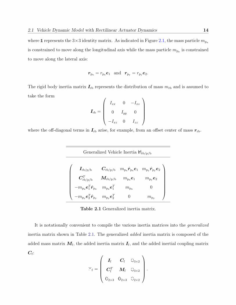
Table 2.1 Generalized inertia matrix.

It is notationally convenient to compile the various inertia matrices into the generalized

inertia matrix shown in Table 2.1. The generalized added inertia matrix is composed of the

added mass matrix Mf , the added inertia matrix If , and the added inertial coupling matrix

Cf :

�f =

If Cf �3×2

CTf Mf �3×2

�2×3 �2×3 �2×2

.


The generalized added inertia matrix accounts for the energy necessary to accelerate the fluid

around the vehicle as it rotates and translates. The inviscid (potential flow) hydrodynamic

parameters are the components of the generalized added inertia matrix and, in notation

similar to that defined by SNAME [34]1, are presented as:

(

If Cf

CTf Mf

)

= −

Lp Lq Lr Lu Lv Lw

Mp Mq Mr Mu Mv Mw

Np Nq Nr Nu Nv Nw

Xp Xq Xr Xu Xv Xw

Yp Yq Yr Yu Yv Yw

Zp Zq Zr Zu Zv Zw

.

The generalized inertia for the vehicle/fluid system is

�= �rb/p/b + �f (2.3)

We define the inertia I, mass M , and coupling C matrices in the following form:

I = Irb/p/b + If

M = Mrb/p/b + Mf

C = Crb/p/b + Cf .

Generalized Velocity (η) Generalized Momentum (ν)

ω

v

rpx

rpy

hsys

psys

ppx

ppy

Table 2.2 Generalized velocity and momentum.

Let psys represent the total linear momentum of the vehicle/fluid system and hsys repre-

sent the total angular momentum. Let ppxand ppy

represent the total translational momen-

1In SNAME notation, roll moment is denoted by K rather than L.


tum of the moving mass particles. Defining the generalized velocity η and the generalized

momentum ν as in Table 2.2, we have

ν = �η. (2.4)

The dynamic equations relate external forces and moments to rates of change of momen-

tum:

hsys = hsys × ω + psys × v + (mrbgrrb +mpxgrpx

+mpygrpy

) × ζ + Tvisc

psys = psys × ω + mgζ + Fvisc (2.5)

ppx= e1 · (ppx

× ω +mpxgζ) + upx

ppy= e2 ·

(ppy

× ω +mpygζ)

+ upy

mb = ub.

The forces upxand upy

can be chosen to cancel to remaining terms in the equations for ppx

and ppy, so that

ppx= upx

ppy= upy

.

These inputs may then be chosen to servo-actuate the point mass positions for attitude

control, although with inherent limits on point mass position and velocity. (Physically, these

actuators might each consist of a large weight mounted on a lead screw that is driven by

a servomotor.) The mass flow rate ub is chosen to servo-actuate the vehicle’s net weight,

again with inherent control magnitude and rate limits. These magnitude and rate limits are

significant for underwater gliders and must be accounted for in control design and analysis.

The terms Tvisc and Fvisc represent external moments and forces which do not derive from

scalar potential functions. These moments and forces include control moments, such as the

yaw moment due to a rudder, and viscous forces, such as lift and drag.


v

®

¯

current axes

w

u

v

Figure 2.2 Illustration of the aerodynamic angles.

The viscous force and moment are most easily expressed in the “current” reference frame.

This frame is related to the body frame through the proper rotation

RBC(α, β) = e−ce2αece3β =

cosα cos β − cosα sin β − sinα

sin β cos β 0

sinα cos β − sinα sin β cosα

.

For example, one may write

v = RBC(α, β)(V e1) =

V cosα cos β

V sin β

V sinα cos β

.

Transformations between various reference frames of interest in vehicle dynamics are

illustrated in Figure 2.3. The most commonly used reference frames are the inertial, body,

and current reference frames, as defined here. Also depicted is the velocity reference frame,

which is related to the current frame through the bank angle µ and to the inertial frame

through the flight path angle γ and the heading angle ζ. (See [2] for details and formal

definitions of µ, γ, and ζ.)

The viscous forces and moments are expressed in terms of the hydrodynamic angles

α = arctan(w

u

)

and β = arcsin( v

V

)

,

where V = ‖v‖. Following standard modeling conventions, we write


InertialReference

Frame

BodyReference

Frame

CurrentReference

Frame

VelocityReference

Frame

ee3Ã e

e2 µ ee1Áe

e2°

ee3 »

ee1¹ ee3 ¯e-e2 ®

Figure 2.3 Rotational transformations between various reference frames. (Adaptedfrom [2].)

Fvisc = −RBC(α, β)

D(α)

Sββ + Sδrδr

Lαα

and Tvisc = Dωω +

Lββ

Mαα

Nββ +Nδrδr

.

The various coefficients, such as Lα and Nβ, depend on the vehicle’s speed, through the

dynamic pressure, the geometry, and the Reynolds number. The matrix Dω contains terms

which characterize viscous angular damping (such as pitch and yaw damping). The expres-

sions above reflect several common assumptions:

• The zero-β side force vanishes.

• The zero-α lift force vanishes and the zero-α viscous pitch moment is zero.

• The viscous lift and side forces are linear in α and β, respectively.

• The viscous drag force is quadratic in lift (and therefore in α).


Equations (2.1), (2.2), and (2.5) completely describe the motion of a rigid underwater

glider in inertial space. In studying steady motions, we typically neglect the translational

kinematics (2.1). Moreover, the structure of the dynamic equations (2.5) is such that we

only need to retain a portion of the rotational kinematics (2.2). Given the “tilt” vector

ζ = RTIBi3, which is simply the body frame unit vector pointing in the direction of gravity,

and referring to equation (2.2), it is easy to see that ζ = ζ ×ω. The reduced set of dynamic

equations, with buoyancy control and moving mass actuator dynamics explicitly represented,

are:

hsys = hsys × ω + psys × v + (mrbgrrb +mpxgrpx

+mpygrpy

) × ζ + Tvisc

psys = psys × ω + mgζ + Fvisc

ζ = ζ × ω (2.6)

ppx= upx

ppy= upy

mb = ub

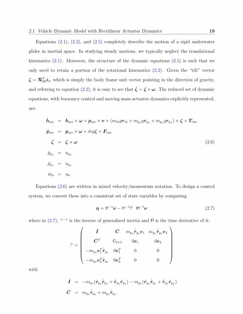
Equations (2.6) are written in mixed velocity/momentum notation. To design a control

system, we convert these into a consistent set of state variables by computing

η = �−1ν − �−1 � �−1ν (2.7)

where in (2.7), �−1 is the inverse of generalized inertia and � is the time derivative of it:

�=

I C mpx˙rpx

e1 mpy˙rpy

e2

CT �3×3 0e1 0e2

−mpxeT1

˙rpx0eT1 0 0

−mpyeT2

˙rpy0eT2 0 0

with

I = −mpx(rpx

˙rpx+ ˙rpx

rpx) −mpy

(rpy˙rpy

+ ˙rpyrpy

)

C = mpx˙rpx

+mpy˙rpy.


2.1.1 Simplified Vehicle Dynamic Model with Rectilinear Actua-

tor Dynamics

As explained in Section 2.1, it is notationally convenient to compile the various inertia

matrices into the generalized inertia matrix shown in Table 2.1. From that we have

�rb/p/b =

Irb/p/b Crb/p/b

0

0

0

0

0

0

CTrb/p/b Mrb/p/b

mpx

0

0

0

mpy

0

(

0 0 0

) (

mpx0 0

)

mpx0

(

0 0 0

) (

0 mpy0

)

0 mpy

The generalized added inertia matrix is composed of the added mass matrix Mf , the added

inertia matrix If , and the added inertial coupling matrix Cf :

�f =

If Cf �3×2

CTf Mf �3×2

�2×3 �2×3 �2×2

The added inertia accounts for energy necessary to accelerate the fluid as the body rotates. If

the underwater glider’s external geometry is such that the b1-b2 and b1-b3 planes are planes

of symmetry, the added inertia matrix is diagonal:

If = −diag

(

Lp Mq Nr

)

.

The added mass matrix accounts for the energy necessary to accelerate the fluid as the body

translates. Like the added inertia matrix, the added mass matrix is diagonal for the class of

underwater gliders considered here:

Mf = −diag

(

Xu Yv Zw

)

.


In addition to the added inertia and the added mass, there will generally be potential flow

and inertial coupling between translational and rotational kinetic energy. For the class of

underwater gliders considered here,

Cf = −

0 0 0

0 0 Mw

0 Nv 0

= −

0 0 0

0 0 Yr

0 Zq 0

T

.

We note that the terms appearing in Cf do not appear in previous glider analysis, al-

though they can be significant.

The generalized inertia for the vehicle/fluid system is

�= �rb/p/b + �f (2.8)

and recall that

I = Irb/p/b + If

M = Mrb/p/b + Mf

C = Crb/p/b + Cf .

Defining the generalized velocity η and the generalized momentum ν as in Table 2.2, we

have

hsys = Iω + Cv + 0rpx+ 0rpy

(2.9)

psys = Mv + CTω +mpxrpx

+mpyrpy

(2.10)

ppx= mpx

e1 · (v + ω × rpx+ rpx

)

= mpxe1 · (v + rpx

) ⇒ mpxrpx

= e1(ppx−mpx

e1 · v) (2.11)

ppy= mpy

e2 · (v + ω × rpy+ rpy

)

= mpye2 · (v + rpy

) ⇒ mpyrpy

= e2(ppy−mpy

e2 · v). (2.12)


From there, we can substitute equations (2.11) and (2.12) into equation (2.10) and obtain

hsys = Iω + Cv

psys = (M − [mpxe1e

T1 +mpy

e2eT2 ])v + CTω + (e1ppx

+ e2ppy) (2.13)

ppx= mpx

e1 · (v + rpx)

ppy= mpy

e2 · (v + rpy).

Defining prb/f = psys − (e1ppx+ e2ppy

), we have

hsys

prb/f

=

I C

CT (M − [mpxe1e

T1 +mpy

e2eT2 ])

ω

v

ppx= mpx

e1 · (v + rpx) (2.14)

ppy= mpy

e2 · (v + rpy)

Let’s call �� =

I C

CT (M − [mpxe1e

T1 +mpy

e2eT2 ])

.

To design a control system, we convert dynamic equations (2.6), presented in mixed

velocity/momentum notation, into a consistent set of state variables considering set of equa-

tions (2.14) into the following form:

ω

v

= ��−1

hsys

prb/f

− ��−1 ��−1

hsys

prb/f

(2.15)

rpx= e1 · (vpx

− v − ω × rpx) (2.16)

vpx=

upx

mpx

+ e1 · (v + ω × rpx+ ω × rpx

) (2.17)

rpy= e2 ·

(vpy

− v − ω × rpy

)(2.18)

vpy=

upy

mpy

+ e2 ·(v + ω × rpy

+ ω × rpy

), (2.19)

where in equation (2.15), prb/f = psys − (e1upx+ e2upy

) and

�� =

−2(mpxrpx

˙rpx+mpy

rpy˙rpy

) mpx˙rpx

+mpy˙rpy

−(mpx˙rpx

+mpy˙rpy

) �3×3

.


2.1.2 Vehicle Dynamic Model with Fixed Actuators

Underwater gliders are so efficient because they spend much of their flight time in stable,

steady motion. In studying steady motions, we do not consider the internal dynamics of the

moving mass actuators. In determining a nominal wings-level glide condition, we assume

that longitudinal moving mass is located at the origin of body fixed reference frame (rpx= 0).

This means that the nominal gravitational moment is due entirely to center of gravity (CG)

location (rrb). For simplicity, we assume that rrb · e2 = 0, so that the vehicle center of mass

(less the contribution of mp) is located in the b1-b3 plane, and we assume that rp = rpe2, so

that the mass mp is located somewhere along the b2-axis.

rp

rrb

b1

b2

b3

i 1

i2

i3

Figure 2.4 Reference frames.

Referring to Figure 2.4, the kinematic equations are

y = RIBv (2.20)

RIB = RIBω (2.21)

The angular momentum of the body/fluid system about the body frame origin is denoted

by the body vector h. The linear momentum of the body/fluid system is denoted by the


body vector p. The vectors h and p are the conjugate momenta corresponding to ω and v,

respectively. To develop expressions for h and p in terms of ω and v requires a number of

definitions.

The inertia matrix I is the sum of three components: the added inertia matrix If , the

rigid body inertia matrix Irb, and a third matrix −mprprp.

I = If + Irb −mprprp.

The mass matrix M is the sum of the added mass matrix Mf and mv�:

M = Mf +mv�.

In addition to the added inertia and the added mass, there will generally be potential

flow and inertial coupling between translational and rotational kinetic energy. The coupling

is characterized by the matrix C = Cf + Crb, where

Crb = mrbrrb +mprp = −CTrb.

The combined rigid body and fluid kinetic energy is therefore

T = Tf + Trb

=1

2

v

ω

T

Mf CTf

Cf If

v

ω

+

1

2

v

ω

T

Mrb CTrb

Crb Irb

v

ω

=1

2

v

ω

T

M CT

C I

v

ω

.

The momenta h and p are defined by the kinetic energy metric and the velocities ω and v:

p

h

=

∂T/∂v

∂T/∂ω

=

M CT

C I

v

ω

. (2.22)

2.2 Vehicle Dynamic Model with Cylindrical Actuator Dynamics 25

The dynamic equations, which relate external forces and moments to the rate of change of

linear and angular momentum, are

p = p × ω + mg(R

TIBi3

)+ Fvisc (2.23)

h = h × ω + p × v + (mpgrp +mrbgrrb) ×(R

TIBi3

)+ Tvisc. (2.24)

Equations (2.20), (2.21), (2.23), and (2.24) completely describe the motion of a rigid

underwater glider with fixed actuators in inertial space. As explained previously in studying

steady motions, given the tilt vector ζ = RTIBi3, we consider the following reduced set of

equations:

ζ = ζ × ω (2.25)

p = p × ω + mgζ + Fvisc (2.26)

h = h × ω + p × v + (mpgrp +mrbgrrb) × ζ + Tvisc. (2.27)

2.2 Vehicle Dynamic Model with Cylindrical Actuator

Dynamics

Figure 2.5 depicts a rigid body (mass mrb) of a glider such as Seaglider with a moving mass

actuator (mp) and a variable ballast actuator (mb). The total vehicle mass is

mv = mrb +mp +mb.

As indicated in Figure 2.5, the variable mass mb is located at the origin of a body-fixed

reference frame. The mass particle mp is constrained to move along the longitudinal axis

(rpx= rpx

e1) and a circle (with radius Rp) in the vertical plane:

rp = rpxe1 +Rp(sin ξe2 + cos ξe3)

ωp = ξe1


rpmp rrb

» rpx

Rp

mb


Define:

er = sin ξe2 + cos ξe3 and eξ = cos ξe2 − sin ξe3.

Hence, in the body frame

rp = rpx+Rper (2.28)

ωp = ξe1,

so the velocity of mp relative to the body is

rp = rpx+ rpωp, (2.29)

where rpωp = Rpξeξ.

Let the body vector vp denote the velocity of the moving mass particle with respect to

inertial space. The kinematic equation for moving mass is

Xp = RIBvp.

Referring to Figure 2.6, let the inertial vector Rp = Xp−X denote the position of the mass

particle relative to the origin of the body frame. An alternative kinematic equation for the

moving mass is

Rp = RIB(vp − v).


rpmp rrb

»

i 1

i2

i3

Xp

X

mb


Finally, define rp = RTIBRp to be the vector Rp expressed in the body frame. This gives the

kinematic equation for moving mass particle

rp = RT

IBRp + RTIB(Xp − X)

= rpω + vp − v

Then, the velocity of the moving mass particle with respect to inertial frame is

vp = v − rpω + rp,

and substituting rp from equation (2.29) gives

vp = v − rpω + rpx− rpωp. (2.30)

Considering the moving mass actuator as a rectangular block with uniformly distributed

mass instead of the particle mass, we need to include the angular momentum of the block

itself about its own center of mass:

Ip(ξ) = Rb1(ξ)TIblockRb1(ξ),


where Iblock represents the principal inertia matrix for the block. Assuming a × b × L

dimensions along (b1, b2, b3) axis,

Iblock =

m12

(b2 + L2) 0 0

0 m12

(a2 + L2) 0

0 0 m12

(a2 + b2)

,

and Rb1(ξ) is a planar rotation about the body’s longitudinal axis,

Rb1(ξ) =

1 0 0

0 cos ξ sin ξ

0 − sin ξ cos ξ

.

Hence the moving mass kinetic energy is

Tp =1

2mpv

2p +

1

2Ip(ξ)(ω + ωp)

2.

Generalized Velocity (η) Generalized Momentum (ν)

ω

v

ωp

rpx

hsys

psys

hp

pp

Table 2.3 Generalized velocity and momentum.

Defining the generalized velocity η and the generalized momentum ν as in Table 2.3, we

have

Tp =1

2ηT�pη, (2.31)

where �p is presented in Table 2.4. The kinetic energy of the rigid-body/moving mass system

is

Trb/p/b =1

2ηT�rb/p/bη. (2.32)


Generalized Moving Mass Inertia �p

Ip(ξ) −mprprp mprp Ip(ξ) +mprprp mprp

−mprp mp� mprp mp�Ip(ξ) +mprprp −mprp Ip(ξ) −mprprp −mprp

−mprp mp� mprp mp�

Table 2.4 Moving mass generalized inertia matrix.

Then the mass, inertia, and inertial coupling matrices for the combined rigid body/moving

mass/variable ballast system is

Irb/p/b = Irb + Ip(ξ) −mprprp

Mrb/p/b = mv�

Crb/p/b = mrbrrb +mprp.

The energy necessary to accelerate the fluid around the vehicle is

Tf =1

2ηT�fη. (2.33)

where the added inertia matrix is in the following form:

�f =

If Cf �3×6

CTf Mf �3×6

�6×3 �6×3 �6×6

.

The total kinetic energy of the system is T = Trb/p/b + Tf . The generalized inertia for the

vehicle/fluid system is

�= �rb/p/b + �f , (2.34)

which is presented in Table 2.5. Then, the generalized momentum can be obtained from

ν =∂T

∂η= �η. (2.35)


Generalized Vehicle/Fluid Inertia �

Irb/p/b + If Crb/p/b + Cf Ip(ξ) +mprprp mprp

CTrb/p/b + CT

f Mrb/p/b + Mf mprp mp�Ip(ξ) +mprprp −mprp Ip(ξ) −mprprp −mprp

−mprp mp� mprp mp�

Table 2.5 Generalized inertia matrix.

The dynamic equations are:

hsys = hsys × ω + psys × v + (mrbgrrb +mpgrp) × ζ + Tvisc

psys = psys × ω + mgζ + Fvisc (2.36)

hp = hp × ω + pp × v +mpgrp × ζ + Tp

pp = pp × ω +mpgζ + Fp

mb = ub,

where Tp and Fp represent moments and forces on moving mass which do not derive from

scalar potential functions. These equations are written in mixed velocity/momentum nota-

tion and they can be converted to a set of dynamic equations in terms of a consistent set of

variables in the following form,

η = �−1ν − �−1 � �−1ν, (2.37)

where �−1 is the inverse of generalized inertia and � is the time derivative of it. Note that

since Ip(ξ) depends on ξ, the computation of the rate of change of the generalized inertia

will be slightly more complicated than was the case for a particle mass.

Chapter 3

Steady Motion

The steady-state flight conditions are determined by solving the nonlinear state equations (2.25–

2.27) for the state and control vectors that make the state derivatives identically zero. Be-

cause of the complexity involved in computing an analytical solution, numerical algorithms

for computing “trim conditions” are common [35]. Here we take an analytical approach

to find (approximate) solutions for steady-state flight in terms of the model parameters

presented in [32] and [31].

Analytical results, approximate or otherwise, are important for motion planning and also

for vehicle design, as they may provide guidelines for sizing actuators and stabilizers. The

conditions for steady turning flight of an underwater glider differ significantly from those

for an aircraft. Deriving a closed-form expression is quite challenging. Instead, we begin

by considering wings level equilibrium flight and consider turning motion as a perturbation.

Given a desired equilibrium speed and glide path angle, one may determine the center of

gravity location and the net weight required. The resulting longitudinal gliding equilibrium

is the nominal solution to a regular perturbation problem in which the vehicle turn rate is

the perturbation parameter.

31

3.1 Wings Level Gliding Flight 32

3.1 Wings Level Gliding Flight

This section summarizes results presented in [21]. The conditions for wings level, gliding

flight are that ω = 0, v ·e2 = 0, and ζ ·e2 = 0. The second condition implies that v = 0 and

therefore that β = 0. The third condition implies that φ = 0. Also, we require that rp = 0

and that δr = 0. Inserting these conditions into equations (2.26) and (2.27) and solving for

the remaining equilibrium conditions gives:

0 = mgζ0 +

−D(α0) cosα0 + Lαα0 sinα0

0

−D(α0) sinα0 − Lαα0 cosα0

(3.1)

0 = Mv0 × v0 + (mrbgrrb) × ζ0 +

0

Mαα0

0

. (3.2)

Following the analysis in [21], one may use equation (3.2) to show that

rrb = r⊥ + %ζ0, (3.3)

where

r⊥ =1

mrbg

Mv0 × v0 +

0

Mαα0

0

× ζ0.

The free parameter % is a measure of how bottom-heavy the vehicle is in a given, wings

level flight condition. This parameter plays an important role in determining longitudinal

stability of the gliding equilibrium. Note that r = r⊥ is a particular solution to the linear

algebraic system,

ζ0r =1

mrbg

Mv0 × v0 +

0

Mαα0

0

,

3.1 Wings Level Gliding Flight 33

obtained from (3.2), for which r⊥ · ζ0 = 0. The null space of ζ0 is described by %ζ0 where

% ∈ �.

Next, one may solve (3.1) for ζ0, v0, and m0 given a desired speed V0 and a desired glide

path angle γ0 = θ0 − α0. Expressed in the inertial frame, equation (3.1) gives

0

0

mg

=

sin (γ0)Lαα0 + cos (γ0)D(α0)

0

cos (γ0)Lαα0 − sin (γ0)D(α0)

. (3.4)

Equation (3.4) states that there is no net hydrodynamic force in the i1-direction and that

net weight is balanced by the vertical components of the lift and drag forces.

The components of viscous force, in the current frame, are

D(α) = PdynSCD(α), S(β) = PdynSCS(β), and L(α) = PdynSCL(α)

where, following standard assumptions, the nondimensional coefficients take the form

CD(α) = CD0+KCL(α)2, CS(β) = CSββ, and CL(α) = CLαα.

The first component of equation (3.4) may be re-written as

tan(γ0) = −CD(α0)

CL(α0)

= −(CD0

+KCL(α0)2

CL(α0)

)

,

which implies that

KC2L + tan(γ0)CL + CD0

= 0. (3.5)

Note that a given glide path angle γ can be obtained, i.e., a real solution CL to equation (3.5)

exists, if and only if

tan2(γ0) ≥ 4KCD0.

Thus, for upward glides (γ0 > 0), one requires that

γ0 ≥ tan−1(

2√

KCD0

)

,

3.2 Steady Turning Flight 34

while for downward glides, one must choose

γ0 ≤ − tan−1(

2√

KCD0

)

.

Clearly, the smaller the product KCD0, the larger the range of achievable glide path angles.

Given values of K and CD0, the best possible glide path angle is

γ0 = (±) tan−1(

2√

KCD0

)

,

This glide path maximizes range (in still water) and corresponds to minimum drag flight:

CL(α0) = ∓√

CD0

K⇒ α0 = ∓ 1

CLα

√

CD0

K.

These conditions provide an upper bound on achievable performance, but operational con-

siderations may dictate a steeper glide path angle.

Having obtained values for CD(α0) and CL(α0) (and for α0 and γ0, and therefore θ0), one

may solve the third component of equation (3.4) for the required net weight m0g for a given

glide speed V0:

m0g =

(1

2ρV 2

0 S

)(cos (γ0)CLαα0 − sin (γ0)

(CD0

+K (CLαα0)2)) . (3.6)

Thus, one may independently assign the glider’s equilibrium attitude, by moving the center

of mass according to (3.3), and its speed, by changing the net weight m0g according to (3.6).

For the minimum drag flight condition, for example,

m0g =

(1

2ρV 2

0 S

)(

∓√

CD0

Kcos (γ0) − 2CD0

sin (γ0)

)

.

3.2 Steady Turning Flight

For turning flight, the condition on ω becomes ω ‖ ζ. One may therefore write

ω = ωζ,

where ω ∈ �is the turn rate. A steady turn is an asymmetric flight condition, so we no

longer assume that v and φ are zero. Moreover, to effect and maintain such an asymmetric

flight condition requires that rp or δr or both be nonzero.


3.2.1 Turning Flight for Aircraft

Before discussing turning flight for an underwater glider, we first review the conditions for

turning flight of aircraft in the notation that we have developed for underwater gliders.

Key differences include the hydrodynamic forces (which, for AUVs, include a significant

contribution from added mass and inertia) and the force of buoyancy. Since there is no

appreciable buoyant force for aircraft, the body frame origin is typically chosen as the center

of mass. In this case, the momenta p and h are related to the velocities v and ω as follows:

p

h

=

mrb� 0

0 I

v

ωζ

. (3.7)

Another important difference between aircraft and underwater gliders is the type of

actuation. Aircraft use control surfaces, such as ailerons, a rudder, and an elevator to

produce control moments, while underwater gliders use the gravitational moment, which

can be adjusted by moving an internal mass.

For an aircraft in a steady turn, equations (2.25) through (2.27) simplify to the following:

ζ = 0 (3.8)

p = 0 = p × ωζ +mrbgζ + Fvisc (3.9)

h = 0 = h × ωζ + Tvisc (3.10)

Note that the first equation implies that ζ is constant, which means that φ and θ are constant.

Also note, in the second equation, that the term p × v has vanished because linear velocity

and momentum are parallel for an aircraft.

The viscous forces and moments will be different from those for an underwater glider,

of course, and they will include terms due to the control surfaces. Thus, terms such as roll

moment due to aileron (Lδaδa) and coupling between the aileron and rudder (Nδaδa and

Lδrδr) must be included. Also, angular rate effects on the aerodynamic force and moment

are included, with standard assumptions concerning vehicle symmetry.


Let T represent thrust, which is assumed to be aligned with the longitudinal axis. Then

Fvisc =

X

Y

Z

= −RBC(α, β)

D(α, β, δa, δe, δr)

Sββ + Sδrδr

Lαα+ Lδeδe

+

T +Xqq

Ypp+ Yrr

Zqq

.

For small sideslip angles,

Y = Yββ + Yδrδr + Ypp+ Yrr.

The viscous moment takes the form:

Tvisc =

Lββ + Lδaδa+ Lδrδr + Lpp+ Lrr

Mαα+Mδeδe+Mqq

Nββ +Nδaδa+Nδrδr +Npp+Nrr

.

For steady turning flight, the components of v and ω are small, with the exception of

u ≈ V . Neglecting products of small terms, one finds that

p × ωζ ≈ mrbV ω

0

− cosφ cos θ

sinφ cos θ

eq

and heq × ωζeq ≈ 0.

Substituting into (3.9) and (3.10), the conditions for steady turning motion of an aircraft

are

0 = mrbV ω

0

− cosφ cos θ0

sinφ cos θ0

+mrbg

− sin θ

sinφ cos θ

cosφ cos θ

+ Fvisc (3.11)

0 = Tvisc. (3.12)

The key condition for steady turning flight is that the lateral aerodynamic force Y be

identically zero [36]. From the second component of equation (3.11), one therefore requires

that

0 = mrbV ω(− cosφ cos θ) +mrbg(sinφ cos θ),


from which the roll angle φ can be obtained in terms of turn rate ω:

tanφ =V

gω. (3.13)

The pitch angle θ, angle of attack α, and pitch rate q may be determined from the

longitudinal components of (3.11) and (3.12), as parameterized by the elevator angle δe and

thrust T . The remaining conditions for steady turning flight are then obtained from the

remaining linear algebraic system:

Yβ Yδr 0

Lβ Lδr Lδa

Nβ Nδr Nδa

β

δr

δa

=

Yp Yr

Lp Lr

Np Nr

ω sin θ

−ω cos θ cosφ

. (3.14)

These equations give the sideslip angle and aileron and rudder deflections necessary for an

aircraft to maintain a banked turn at a given speed V , turn rate ω, and pitch angle θ.

3.2.2 Turning Flight for Underwater Gliders

The situation for an underwater glider is considerably different. The center of mass is no

longer the origin of the body reference frame and angular and linear momentum are cou-

pled through inertial asymmetries. Linear momentum is no longer parallel to linear velocity,

because added mass is directional and because of coupling between linear and angular ve-

locity introduced by the offset center of mass. Propulsion is provided not by a thruster

but by the net weight of the vehicle (weight minus buoyant force). In fact, the problem of

finding analytical steady turning solutions for underwater gliders is quite challenging. We

instead formulate the problem as a regular perturbation problem in the turn rate and seek

a first-order approximate solution. To argue that the higher order solutions are “small cor-

rections” requires some well-founded notion of “small,” so we begin by nondimensionalizing

the dynamic equations.

We choose the reference parameters

length: l, mass: mrb, and time: T =l

V0

,


where l is a characteristic length scale for the vehicle (such as length overall) and V0 is the

nominal speed. With these definitions, the nondimensional momenta p and h are related

to the nondimensional velocities v and ω through the nondimensional generalized inertia

matrix as follows:

p

h

=

M CT

C I

v

ω

where

v =1

V0

v and ω = ωT

and where

M =1

mrb

M , I =1

mrbl2I, and C =

1

mrblC.

The nondimensional dynamic equations are

˙ζ = ζ × ω (3.15)

˙p = p × ω + ¯mζ + Fvisc (3.16)

˙h = h × ω + p × v + (mprp + rrb) × ζ + Tvisc, (3.17)

where the overdot represents differentiation with respect to nondimensional time T and

where

ζ =ζ

V 20 /(gl)

, ¯m =m

mrb

, mp =mp

mrb

, rrb =rrb

l, and rp =

r

l

and

Fvisc =Fvisc

mrbV 20 /l

and Mviscous =Tvisc

mrbV 20

.

To express the viscous forces and moments explicitly, we also define

V =V

V0

, ρ =ρ

mrb/l3, and S =

S

l2.

To simplify the analysis, we assume that

Dω =1

2ρV 2S diag

(Clp , Cmq , Cnr

)


where Clp , Cmq , and Cnr are nondimensional stability derivatives representing rotational

damping. The assumption that roll and yaw damping are decoupled is reasonable for a

vehicle with two planes of external geometric symmetry.

Recall that ω = ωζ for a steady turn. Define a characteristic frequency ωn =√

g/l and let

ωn = ωnT denote its nondimensional value. Let ω = εωn where ε is a small, nondimensional

parameter. One may treat the problem of solving for steady turning flight conditions as

an algebraic regular perturbation problem in ε. When ε = 0, the vehicle is in wings-level

equilibrium flight. If ε 6= 0, then either rp or δr or both must be nonzero. (Recall that

rrb remains fixed at its nominal value, which corresponds to the nominal wings-level flight

condition when rp and δr are zero.)

Having nondimensionalized the terms appearing in the dynamic equations, we simplify

notation by omitting the overbar; in the sequel, all quantities are nondimensional unless

otherwise stated. The nondimensional equilibrium equations are

0 = peq × ωζeq + meqζeq −(

1

2ρV 2

eqS

)

RBC(αeq, βeq)

CD(α)

CSββ

CLαα

eq

0 = heq × ωζeq + peq × veq + (mprp + rrb) × ζeq +

(1

2ρV 2

eqS

)

Clββ

Cmαα

Cnββ + Cnδrδr

eq

+Dωωζeq

where Clβ , Cmα , Cnβ , and Cnδr are nondimensional stability derivatives. Note that

peq

heq

=

M CT

C I

veq

(ωζeq)

where

veq = RBC(αeq, βeq)(Veqe1).


As we have stated, ζ remains constant in turning flight; equivalently, φ and θ remain

constant. We seek equilibrium solutions for which the perturbed value of ζ takes the following

form:

ζeq = e−φeqce1ζ0

=

1 0 0

0 cosφeq sinφeq

0 − sinφeq cosφeq

ζ0.

By construction, the perturbed equilibrium turning motion will have the same pitch angle θ

as the corresponding, unperturbed wings level flight condition.

Using the definitions and observations above, the equilibrium equations may be written

more explicitly:

0 =(

M (RBC(αeq, βeq)(Veqe1)) + CT(

εωne−φeqce1ζ0

))

×(

εωne−φeqce1ζ0

)

+meqe−φeqce1ζ0 −

(1

2ρV 2

eqS

)

RBC(αeq, βeq)

CD(α)

CSββ

CLαα

eq

(3.18)

0 =(

I(

εωne−φeqce1ζ0

)

+ C (RBC(αeq, βeq)(Veqe1)))

×(

εωne−φeqce1ζ0

)

+(

M (RBC(αeq, βeq)(Veqe1)) + CT(

εωne−φeqce1ζ0

))

× (RBC(αeq, βeq)(Veqe1))

+ (mprp + rrb) ×(

e−φeqce1ζ0

)

+ Dω

(

εωne−φeqce1ζ0

)

+

(1

2ρV 2

eqS

)

Clββ

Cmαα

Cnββ + Cnδrδr

eq

. (3.19)

To obtain the regular perturbation solution in ε, first substitute the following polynomial

expansions for rp, m, φ, V , α, and β:


V =∑

n

Vnεn = V0 + εV1 + ε2V2 + · · ·

α =∑

n

αnεn = α0 + εα1 + ε2α2 + · · ·

β =∑

n

βnεn = εβ1 + ε2β2 + · · ·

m =∑

n

mnεn = m0 + εm1 + ε2m2 + · · ·

φ =∑

n

φnεn = εφ1 + ε2φ2 + · · ·

rp =∑

n

rpnεn = εrp1

+ ε2rp2+ · · ·

(We have suppressed the subscript “eq” for convenience.) Also, let δr = 0 + εδr1. (The rud-

der deflection δr1 will appear as a free parameter in the solution to the regular perturbation

problem.) Substituting these polynomial expansions into equations (3.18) and (3.19) and

collecting powers of ε gives a regular perturbation series in ε. Solving the coefficient equation

for ε0 gives the nominal, wings level flight conditions. Solving the coefficient equation for ε1

gives approximate values for rp, m, φ, V , α, and β to first order in ε. Let

∆ = (ρS)2 (rbxcθ0 + rbzsθ0)(CD(α0) + CSβ

)+ m0 (ρS)

(Cnβcθ0 − Clβsθ0

)

+2m0 [(−Xu + Yv) cα0cθ0 + (−Zw + Yv) sα0sθ0] , (3.20)

where “s” represents the sine function and “c” represents cosine. The first-order solution to

the regular perturbation problem defined by equations (3.18) and (3.19) is:

V1 = 0 (3.21)

α1 = 0 (3.22)

m1 = 0 (3.23)

β1 = −ωn∆

{2 (rbxcθ0 + rbzsθ0) [(m−Xu) cα0cθ0 + (m− Zw) sα0sθ0] + 2m0cθ0c(θ0 − α0)Nv

+m0 (ρS)(Clps

2θ0 + Cnrc2θ0

)}− ρS

∆[m0cθ0Cnδrδr1 + (rbxcθ0 + rbzsθ0)CSδrδr1]

(3.24)

φ1 =ωn

4m0cθ0∆[(m+ m0 −Xu) cα0cθ0 + (m+ m0 − Zw) sα0sθ0]

+ρS

8m0cθ0

[(CD(α0) + CSβ

)β1 +

1

∆CSδrδr1

]

(3.25)


rp1=

1

2mp∆

{2ωn (ρS)

(rbxClβ + rbzCnβ

)[(m−Xu) cα0cθ0 + (m− Zw) sα0sθ0]

+2m0ωn (ρS)[Clp (−Xu + Yv) cα0sθ0 − Cnr (−Zw + Yv) sα0cθ0

]

+2ωns2α0 (−Zw + Yv) [rbx (m−Xu) cθ0 + rbz (m− Zw) sθ0]

−2ωn (1 − c2α0) [rbx (m− Zw) (−Zw + Yv) sθ0 − rbz (m−Xu) (−Xu + Yv) cθ0]

−4m0ωnsα0 {[Mw (−Xu + Yv) +Nv (−Xu + Zw)] cα0sθ0 −Mw (−Zw + Yv) sα0sθ0}

+ωn (ρS){[m0Clβ − rbz

(CD(α0) + CSβ

)][(ρS)Cnrcθ0 + 2 (Nvcα0cθ0 −Mwsα0sθ0)]

+[m0Cnβ + rbx

(CD(α0) + CSβ

)] [(ρS)Clpsθ0 + 2 (Mw +Nv) sα0cθ0

]}

+ (ρS)Cnδrδr1{(ρS)

[m0Clβ − rbz

(CD(α0) + CSβ

)]− 2m0 (−Zw + Yv) sα0

}

+ (ρS)CSδrδr1{(ρS)

(rbxClβ + rbzCnβ

)+ 2 [rbx (−Zw + Yv) sα0 + rbz (−Xu + Yv) cα0]

}}

(3.26)

The explicit analytical expressions given above, particularly in equations (3.24–3.26),

provide insight concerning the role of design parameters such as wing sweep angle, vertical

stabilizer size, moving mass actuator size, and rudder size in determining a vehicle’s turning

capability. They also exhibit an interesting structure, which is discussed in Remark 3.2.1

below.

Remark 3.2.1 That V , α, and m remain constant to first order in ε suggests that the

primary contributors to steady turning motion are lateral mass deflections (rp) and rudder

deflections (δr1) and that these deflections have no first-order effect on speed or angle of

attack. In practice, it is considerably more costly to change the vehicle’s net mass m than

to shift its center of gravity. As shown in equation (3.6), m directly controls speed, so to

maximize glider speed in descent (ascent) one must drive m to its maximum (minimum)

value. Thus, at least in maximum speed operations, the problem of controlling longitudinal

motion (speed and glide path angle) decouples from the problem of controlling directional

motion (turn rate) to first order in ε. As it will be discussed in Section 6.1, this observation

suggests a natural approach to motion control and path planning for underwater gliders.

3.3 Numerical Case Study: Slocum 43

Remark 3.2.2 Note that the rudder deflection δr1 appears as a free parameter in expres-

sions (3.21–3.26). For a rudderless vehicle, one simply sets δr1 = 0. Including a rudder,

however, provides additional freedom to control the lateral-directional dynamics. For exam-

ple, using (3.24), one could adjust the rudder angle so as to zero the sideslip angle, to first

order in ε, thereby reducing the total drag. (Equation (3.24) gives guidance for sizing a

rudder for this purpose.) Drag reduction is especially critical for underwater gliders, whose

primary operational advantage is efficiency. On the other hand, a rudder is an external ac-

tuator which is subject to damage or fouling and which introduces an additional failure mode

into the system.

Equations (3.21–3.26) provide a first-order approximation for steady turning motions. To

assess stability of the true, neighboring turning motion, one may linearize about the approx-

imate equilibrium condition and compute the eigenvalues. Recognizing that the eigenvalues

of the resulting time-invariant state matrix depend continuously on its parameters, stability

properties of the true equilibrium may be inferred from stability properties of the approxi-

mate equilibrium provided that (i) the equilibrium is hyperbolic and (ii) ε is small relative

to the real part of every eigenvalue. See Section 1.7 of [37] for a brief discussion or Chapter 9

of [38] for more details.

3.3 Numerical Case Study: Slocum

To verify our steady turn predictions for a realistic vehicle model, we have applied the results

to the model for Slocum, shown in Figure 3.1, for which hydrodynamic model parameters

are given in [26]. We consider perturbations from a wings-level equilibrium flight condition

at speed V0 = 1.5 knots and angle of attack α0 = 4.3◦, the angle which corresponds to the

maximum lift-to-drag ratio. We assume that δr1 = 0, noting that neither Liberdade/XRay

nor the deep-water (“thermal”) version of Slocum uses a rudder.

Figure 3.2 shows the wings-level equilibrium glide characteristics for the Slocum glider.


Figure 3.1 The underwater glider Slocum. (Solid model in Rhinoceros 3.0.)

−30 −20 −10 0 10 20 30−80

−60

−40

−20

0

20

40

60

80

α ( o )

γ (

o ),θ

( o )

γθ

−80 −70 −60 −50 −40 −30 −20 −10 0−80

−70

−60

−50

−40

−30

−20

−10

0

10

20

γ ( o )

θ (

o )

Figure 3.2 Wings level equilibrium glide characteristics for Slocum model.

The lift, sideforce and drag parameters are:

CLα = 2.04 rad−1, CSβ = 0.30 rad−1, CD0= 0.03, and K = 0.16.

Other important parameters include l = 1.5 m and mrb = 40 kg. The rigid body inertia

matrix is

Irb =

0.25 0 0

0 9.72 0

0 0 9.72

.

The values of the nonzero terms in the generalized added mass matrix are given below.


−Xu = 5 kg

−Yv = 60 kg

−Zw = 70 kg

−Lp = 3.75 kg-m2

−Mq = 2.28 kg-m2

−Nr = 1.28 kg-m2

The values of the viscous stability derivatives are given below.

Cm

α −0.75

q −0.90

Cl

β −0.90

p −0.30

Cn

β 1.51

r −0.30

Once one has computed the conditions for equilibrium flight, one may examine stability.

The simplest approach is spectral analysis. Using the Slocum model described in [26], we

linearize about the wings-level, equilibrium flight condition corresponding to the following

parameter values:

V0 = 0.758 m/s, α0 = 4.3◦, θ0 = −8.2◦, γ0 = −12.5◦ and m0 = 0.61 kg.

As mentioned in Section 3.1, the free parameter % provides a measure of how bottom-heavy

the vehicle is, in a given flight condition. This parameter plays an important role in deter-

mining longitudinal stability of wings-level gliding equilibria. The effect of varying % on the

stability of wings-level and turning equilibria has been investigated numerically. The results

show that the equilibrium condition mentioned above is stable provided % > 0.05, which

agrees with the analysis in Section 8.3 of Bhatta’s dissertation [26]. Here, the value of % is

fixed at 0.117, as in [26].

The eigenvalues of the state matrix corresponding to the given equilibrium condition are

λ ∈ {−4.46,−2.67 ± 1.64i,−1.26,−1.03,−0.75 ± 0.25i,−0.07}

All eight eigenvalues of the linearized system have negative real part, so the flight condition

is stable.


0200

400600

800

−1

−0.5

0

0.5

1

0

50

100

150

x (m)y(m)

z (m

)

−40−20

020

40

−20

0

20

40

60

0

50

100

150

x (m)y(m)

z (m

)

Figure 3.3 Wings level (ε = 0) and turning (ε = 0.01) flight paths for the Slocummodel.

−5 −4 −3 −2 −1 0−3

−2

−1

0

1

2

3

Real Axis

Imag

inar

y A

xis

ActualApproximate

−1 −0.8 −0.6 −0.4 −0.2 0−0.5

−0.4

−0.3

−0.2

−0.1

0

0.1

0.2

0.3

0.4

0.5

Real Axis

Imag

inar

y A

xis

ActualApproximate

Figure 3.4 Eigenvalue plots for actual and approximate equilibria for 0 < ε < 0.1.(A closer view of the dominant eigenvalues is shown at the right.)

With stability of wings-level equilibrium flight confirmed, one may next compute the

first-order solution for rp, φ, and β, as described in Section 3.2:

rp = (4.63ωnε) m, φ = (10.06ωnε)

(180

π

)

deg, and β = (0.33ωnε)

(180

π

)

deg.

With these approximate values for lateral mass location, roll angle, and sideslip angle, the


approximate equilibrium velocity and angular velocity are

v = V0

cosα0 cos (εβ1)

sin (εβ1)

cosα0 sin (εβ1)

and ω = ωnε

sin θ0

cos θ0 sin (εφ1)

cos θ0 cos (εφ1)

.

When ε = 0, the values above correspond to the given, steady, wings-level flight condition.

For small, nonzero values of ε, the values correspond (approximately) to a steady turning

motion; see Figure 3.3. To determine the range of stable turning motions that can be obtained

using this approximation, the equations of motion are linearized about the approximate

turning motion, parameterized by ε. When ε = 0, all eight eigenvalues of the linearization

have negative real part, with λ8 = −0.07 being closest to the imaginary axis. As ε increases,

this eigenvalue moves to the left along the real axis. The other critical eigenvalues start

as a conjugate pair from λ6,7 = .75 ∓ .25i. As ε increases, they move toward together to

the right and break away when they meet on the real axis. One moves to the left and the

other moves to the right along the real axis, which coalesces with λ8 and then breaks away

into a complex conjugate pair. One may infer that the system has a locally unique, stable

fixed point provided ε remains smaller in order of magnitudes than the magnitude of the real

part of the critical eigenvalue(s) [38]. Figure 3.4 shows the movement of eigenvalues for the

approximate equilibrium as well as those for the true equilibrium (computed numerically) as

ε increases from zero. The true and approximate root loci agree very closely for ε < 0.03. The

true system exhibits a stable turning motion for 0 < ε < 0.1. Table 3.1 gives approximate

and actual values (obtained from numerical simulations) for key variables for various values

of ε. Note that, as ε increases in value, so does the error between the approximate and true

equilibrium values. Regardless, the system does converge to a steady turning motion for all

values ε ≤ 0.1.

Remark 3.3.1 Note in Table 3.1 that the actual turn radius R is minimum around ε = 0.05.

Since further increases in rp (or equivalently in ε) fail to lower the turn radius, there is no

point in moving the particle mp beyond this critical location. Such an observation may provide


Table 3.1 Approximate and actual steady motion conditions for V0 = 1.5 knotsand α= 4.3◦.

ε φ (◦) β (◦) θ (◦) V (m/s) ω (rad/s) R (m)

app. actual app. actual actual† actual† app. actual app. actual

0.001 1.47 1.43 0.05 0.12 -8.74 0.77 0.003 0.003 253.33 256.67

0.005 7.37 7.11 0.24 0.61 -8.82 0.78 0.013 0.014 58.46 55.71

0.01 14.73 13.89 0.49 1.28 -9.03 0.79 0.026 0.027 29.23 29.26

0.03 44.21 34.99 1.46 4.37 -9.8 0.87 0.077 0.057 9.87 15.26

0.05 73.69 47.84 2.43 6.99 -9.69 0.93 0.128 0.063 5.94 14.76

0.07 103.16 56.04 3.40 8.94 -9.01 0.97 0.179 0.060 4.25 16.17

†The approximate value of θ is θ0 = −8.24◦. The approximate value of V is V0 = 0.758 m/s.

guidelines for actuator sizing in future glider designs. There is no reason, for example, to

provide moving mass control authority which does not yield greater turning ability.

Comparing the results for speeds of 1.0, 1.5, and 2.0 knots (illustrated in Tables 3.3, 3.1,

and 3.2, respectively), one may observe several trends. For example, in every case, actual

speed increases with increasing turn rate. (Recall that the approximation suggests that

speed remains relatively constant, for small ε.) Roll angle and sideslip angle (approximate

and actual) increase more rapidly with turn rate at lower nominal speeds than at higher

nominal speeds. Moreover, the discrepancy between the approximate and actual values is

greatest (for given ε) at the lowest speed. Because the relative stability of the nominal flight

condition decreases with decreasing speed (i.e., the critical eigenvalues move closer to the

imaginary axis), one should expect poorer agreement between the approximation and reality

at these lower speeds.


Table 3.2 Approximate and actual steady motion conditions for V0 = 2.0 knotsand α= 4.3◦.

ε φ (◦) β (◦) θ (◦) V (m/s) ω (rad/s) R (m)


0.001 0.87 0.89 0.06 0.06 -8.02 1.002 0.003 0.003 337.00 334.00

0.005 4.34 4.42 0.29 0.29 -8.08 1.004 0.013 0.013 77.77 77.23

0.01 8.69 8.74 0.63 0.58 -8.24 1.011 0.026 0.026 39.55 39.33

0.03 26.06 23.85 2.29 2.29 -9.41 1.069 0.077 0.065 13.18 16.49

0.05 43.43 34.88 3.38 3.55 -10.41 1.144 0.128 0.085 7.91 13.46

0.07 60.80 42.80 4.70 4.92 -10.88 1.207 0.179 0.093 5.65 12.94


Table 3.3 Approximate and actual steady motion conditions for V0 = 1 knot andα= 4.3◦.

ε φ (◦) β (◦) θ (◦) V (m/s) ω (rad/s) R (m)


0.001 2.93 2.77 0.01 0.28 -9.26 0.52 0.003 0.003 170.00 173.33

0.005 14.64 13.54 0.02 1.71 -9.31 0.53 0.013 0.015 39.23 35.33

0.01 29.28 25.42 0.03 3.43 -9.32 0.55 0.026 0.027 19.78 20.92

0.02 58.55 42.70 0.11 9.66 -8.74 0.60 0.051 0.034 9.89 17.99

0.03 87.83 53.54 0.17 12.61 -7.74 0.63 0.077 0.033 6.59 19.51

0.04 117.10 60.65 0.23 13.75 -6.75 0.65 0.102 0.029 4.95 22.03


Chapter 4

Motion Control

Having characterized steady turning motions (at least approximately) in Section 3.2.2 as

well as steady, wings level flight in Section 3.1, one can formulate a motion control strategy

which relies on these solutions. The aim is to track desired speed (Vd), glide path angle

(γd), and turn rate (ψd). Given feasible values for desired speed, glide path angle, and

turn rate, for example, one may compute “feedforward” actuator commands to adjust the

net weight and center of gravity in order to achieve the given flight condition. Because

these values are only approximate, though, and because of modeling and environmental

uncertainty, the commanded values must be augmented using feedback compensation. The

design and analysis of such a feedforward/feedback motion control system requires a model

that incorporates buoyancy and moving mass actuator dynamics as presented in Section 2.1.

An illustration of such a feedforward/feedback control system is shown in Figure 4.1. The

vector field f(x,u) represents the system dynamics with state vector x and inputs u, and

the vector field f(x,u) notionally represents their first-order approximation in turn rate.

The pair (xeq, ueq) represents the first-order solution for a given desired steady motion. The

vector µ contains parameter values which, if held constant, correspond to some stable steady

motion. Such a feedforward/feedback motion control system was briefly presented in [33]; a

more thorough discussion of the design and analysis was presented in [39].

50

51

Figure 4.1 A steady motion-based feedforward/feedback control system.

The first step in the motion control scheme is to obtain the parameter values µd (net mass

and moving mass positions) that correspond to the desired steady motion xeq (characterized

by Vd, γd, and ψd), to first order in turn rate. This inverse problem is expressed notationally

in the feedforward block in Figure 4.1 by the equation

0 = f(xeq, ueq),

which was solved analytically for the corresponding parameter values µd in [32].

The feedback block compensates for the error due to the approximation and environmen-

tal uncertainty, adding a correction denoted µcorr.

The feedback-compensated “parameter commands” µd are then realized within the ve-

hicle dynamics

x = f(x; u(x; µd))

through an appropriately designed servo-control system. Here, u is a feedback control law

that attempts to maintain commanded parameter values µd in spite of the vehicle dynamics.

The control system depicted in Figure 4.1 suggests that one may vary the steady motion

according to some desired guidance objective. However, one must verify that the closed-loop

system is stable. Fixing parameter values, one may examine open-loop stability by linearizing

about the approximate equilibrium conditions and computing the eigenvalues of the state

52

matrix. Because eigenvalues depend continuously on the matrix parameters, stability of the

true equilibrium may be inferred from stability of the approximate equilibrium provided (i)

the equilibrium is hyperbolic and (ii) ε is small relative to the magnitude of the real part

of each eigenvalue. See Section 1.7 of [37] for a brief discussion or Chapter 9 of [38] for

more details. Given that the system does possess a stable, steady motion parameterized by

a set of commanded parameter values, one must still verify that the system remains stable

while varying these parameter values. For example, if one changes the reference commands

in Figure 4.1 too rapidly, one might drive the nonlinear system into instability.

As explained earlier, underwater gliders steer by moving one or more internal masses.

The vehicle dynamics are quite slow, relative to the actuator dynamics. Commanding a rapid

change in turn rate, for example, will result in a quick change in center of mass location, but

the resulting effect on the vehicle’s motion will be much slower. Alternatively, one may issue

reference commands that vary “quasisteadily” and treat the closed-loop system as “slowly

varying” in the turn rate ψd(t). We may then analyze stability of the closed-loop system in

the context of slowly varying systems theory [40].

Suppose the output of a nonlinear system

x = f(x, upy) ; upy

= κ(x, ψd)

is required to track a reference input ψd(t), where the feedback controller κ is designed such

that the closed-loop system has a locally exponentially stable equilibrium at xeq when ψd(t)

is constant. The turn rate ψd(t) is called “slowly varying” if it is continuously differentiable

and, for some sufficiently small ε > 0, one has ‖ψd(t)‖ ≤ ε for all t ≥ 0.

We will analyze the underwater glider’s motion control system using slowly varying sys-

tems theory to prove stability of the closed-loop system and, simultaneously, to determine

how fast one may vary the commanded turn rate and maintain stability.

To analyze this system, consider ψd as a “frozen” parameter and assume that for each

fixed value the frozen system has an isolated equilibrium point defined by xeq = h(ψd) where

‖ ∂h∂ψd

‖ ≤ L. To analyze stability of the frozen equilibrium point, we shift it to the origin via

4.1 Feedforward/Feedback Controller Design 53

the change of the variables x = x − h(ψd) to obtain equation

˙x = g(x).

Based on Theorem 9.3 of Khalil [40], if there is a positive definite and decrescent Lyapunov

function V (x) that has a negative definite derivative along the trajectories of the system,

and which satisfies certain inequalities to handle the perturbation –and the fact that ψd(t)

is not constant–, the solution will be uniformly ultimately bounded within a ball around

the equilibrium point, with a radius proportional to ε, for sufficiently small ε. Moreover, if

ψd(t) → 0 as t→ ∞, then the tracking error tends to zero.

4.1 Feedforward/Feedback Controller Design

The feedforward block takes the commanded steady motion parameters (speed, glide path

angle, and turn rate) and generates the corresponding values for buoyancy and center of

mass location, as predicted by perturbation analysis. Because the turning motion results are

only approximate, however, and to compensate for model and environmental uncertainty, we

incorporate feedback. The objective here is to design single-input, single-output PID control

loops to modify the feedforward commands based on measured errors in the values of speed

V , glide path angle γ = θ − α, and heading rate ψ = sinφcos θ

q + cosφcos θ

r. Speed and glide path

angle are inherently coupled for underwater gliders, just as they are for airplanes. For a fixed

glide path angle, speed can be directly modulated by changing the net mass m. Changing m

requires pressure-volume work, however, which is relatively expensive, especially at depth.

In practice, it is best to modulate m as infrequently as possible. Here, we focus on controlling

the glide path angle γ by varying the longitudinal moving mass position rpx.

A sophisticated dynamic model presented in Section 2.1 has been used to design the

feedback compensator. The model incorporates the buoyancy and moving mass actuator

dynamics and servo-control laws. It is convenient to replace the velocity v, as expressed in

the body reference frame, with speed, angle of attack, and sideslip angle (V, α, β). To do so,


note that

v = e−ce2αece3β(V e1)

v = e−ce2αece3β

1 0 0

0 0 V

0 V cos β 0

V

α

β

.

The change of variables is well-defined for β ∈ (−π2, π

2).

The equations of motion (2.7) can be written in the form

�(�,�, �) = 0

where the system state and control vectors are

�=

[φ, θ, V, α, β, p, q, r, rpx

, vpx, rpy

, vpy

]T

� =[upx

, upy, ub

]T.

Note that vpxand vpy

represent the translational velocity of the moving masses relative to

the inertial frame expressed in the body frame.

To design a servo-controller for the moving mass actuators and the variable ballast ac-

tuator, we linearize the dynamic equations about a wings-level equilibrium (�

0, �0) and

compute the transfer function for each input-output channel of interest. Let U denote one

of the available input signals U ∈{upx

, upy, ub

}and define a corresponding output Y (

�).

With these definitions, we obtain the perturbation equations

4�= A4�

+ B4U (4.1)

4Y = C4�(4.2)

where

A = −[(

∂�

∂�)−1(

∂�

∂�)]

eq

B = −[(

∂�

∂�)−1(

∂�

∂U

)]

eq

C =

[∂Y

∂�]

eq

.


The matrix ∂�∂ is non-singular within the vehicle’s normal performance envelope.

In designing moving mass servo-controllers, the objective is to choose an input up ∈

{upx , upy} such that the position of the moving mass rp ∈ {rpx , rpy} asymptotically tracks a

desired trajectory rpd∈ {rpxd , rpyd}. With U = up and Y = rp in equations (4.1) and (4.2),

the scalar CAB is nonzero. Let e = rpd−rp represent the error between the desired position

of a moving mass and its current position. In order to drive e to zero, one may choose

up =1

CAB(rpd

− CA24�+ [ω2

n 2ζωn]e),

where e = [e, e]T and where ωn ∈ {ωnx , ωny} and ζ ∈ {ζx, ζy} are appropriately chosen control

parameters, assuming that rpdis twice differentiable.

To design a PID compensator to correct the feedforward commands, letG(s) represent the

transfer function for a particular control channel and let Gc(s) represent the PID controller:

Gc(s) = Kp(1 +1

Tis+ Tds).

The proportional gain Kp, the integrator time Ti, and the derivative time Td are control

parameters to be tuned by the control designer. In the time domain, the control signal is

rcorrp = Kpe+Ki

∫ t

t0

e(τ)dτ +Kde,

where Ki = Kp/Ti and Kd = KpTd. The error signal e(t) measures the difference between

the actual and commanded value of the output.

The approximate equilibrium value of rpd∈ {rpxd , rpyd}, as predicted by analytical solu-

tions, is augmented with feedback compensation to compensate for approximation error:

rpd= rpd

+ rcorrp .

To smooth the commanded parameter value so that the reference command to the internal

servo-actuators is twice differentiable, we define a linear reference model:

F (s) : rpd→ rcomm

pdwhere F (s) =

1

(s/ωr)2 + 2ζr(s/ωr) + 1.


Equivalently, in time domain, define the following reference model dynamics for each servo-

actuator:

z =

0 1

−ω2r −2ζrωr

z +

0

ω2r

rpd

rcommpd

=

(

1 0

)

z

where rpd(t) ∈ {rpxd

(t), rpyd(t)} is the (possibly discontinuous) reference command to be

filtered.

In physical implementations, the servo-actuation system is self-contained and there is no

need to include it in the motion control system. Referring to the control system schematic in

Figure 4.1, this reference command filter is internal to the system dynamics block appearing

at the right. We include this element explicitly here in order to account for the full com-

plexity of the multi-body mechanical system and to allow analysis of issues such as actuator

magnitude and rate saturation. Actuator rate and magnitude saturation can be important

issues for underwater gliders. The natural frequency and damping ratio parameters in the

reference model above may be chosen to accommodate actuator performance limitations

through analysis and simulation.

For a fixed glide path angle, speed can be directly modulated by changing the net mass

m. That is, given values θ0 and γ0, one may solve relation (3.6) for the corresponding values

of md. We design an input ub such that the net mass m asymptotically tracks a desired

value md. The simplest approach is to choose

ub = kb (md − m)

where the constant kb is chosen to accommodate the rate limit on ub.

4.2 Flight Path Control 57

4.2 Flight Path Control

We control the glide path angle γ by modulating the longitudinal moving mass position rpx.

Let eγ(t) = γd − γ(t), where γd is the desired value of the glide path angle. The longitudinal

moving mass reference signal is

rcorrpx

= Kpγeγ +Kiγ

∫ t

t0

eγ(τ)dτ +Kdγ eγ.

The first step is to tune the flight path controller for the linearized system dynamics. Having

done so, the next step is to re-tune the controller as necessary for the nonlinear dynamics

through simulation. Adding the result to the longitudinal moving mass position from the

feedforward block gives the required position of the longitudinal moving mass to maintain a

constant flight path angle:

rpxd= rpxd

+ rcorrpx

.

As explained in Section 2.1.2 we assumed that the nominal gravitational moment is due

entirely to rrb and that rpxd= 0. Hence, for γd = γ0, we have only the feedback term

rpxd= rcorr

px.

The reference command should be filtered to accommodate the magnitude and rate limit

on the longitudinal moving mass actuator due to limited range of travel of the moving mass

and the operational limit of the servomotor driving it:

rcommpxd

=

(

1 0

)

zx where zx =

0 1

−ω2rx −2ζrxωrx

zx +

0

ω2rx

rpxd

(t).

The input upxguarantees that the position of the longitudinal moving mass rpx

asymp-

totically tracks the (twice-differentiable) trajectory rcommpxd

generated by filtering (possibly

discontinuous) desired value rpxd:

upx=

(rcommpxd

− CxA2X + [ω2

nx2ζxωnx

]ex)

CxABx

where ex = (ex, ex)T & ex = rcomm

pxd− rpx

.

4.3 Turn Rate Control 58

4.3 Turn Rate Control

The channel from lateral mass position rcorrpy

to turn rate ψ is non-minimum phase, with a

single zero in the right half plane. This non-minimum phase zero limits closed-loop band-

width. In any case, closing the loop from turn rate to lateral mass location is quite effec-

tive, provided the performance limitations are respected in control parameter selection. Let

eψ(t) = ψd(t) − ψ(t), where ψd(t) is the desired turn rate. The lateral moving mass control

signal is

rcorrpy

= Kpψeψ +Ki

ψ

∫ t

t0

eψ(τ)dτ +Kdψeψ.

The turn rate PID controller was first tuned for the linearized system dynamics, and then

re-tuned for the nonlinear dynamics through simulation. Adding the result to the lateral

moving mass position from the feedforward block gives the required position of the lateral

moving mass to maintain the desired turn rate:

rpyd= rpyd

+ rcorrpy

.

The reference command should be filtered to accommodate magnitude and rate limits on

the lateral moving mass actuator due to the limited range of travel of battery pack and the

operational limit of servomotor driving it:

rcommpyd

=

(

1 0

)

zy where zy =

0 1

−ω2ry −2ζryωry

zy +

0

ω2ry

rpyd

(t).

The input upyguarantees that the position of the lateral moving mass rpy

asymptotically

tracks the (twice-differentiable) trajectory rcommpyd

generated by filtering (possibly discontinu-

ous) desired value rpyd:

upy=

(rcommpyd

− CyA2X + [ω2

ny2ζyωny

]ey)

CyABy

where ey = (ey, ey)T & ey = rcomm

pyd− rpy

.

4.4 Stability Analysis of Closed-Loop System 59

4.4 Stability Analysis of Closed-Loop System

To analyze this system, consider ψd as a frozen parameter. For each fixed value the frozen

system has an isolated equilibrium point. Consider the linearized equations about this

equilibrium point:

�= A

�+ Byupy

rpy= Cy

�,

where�

is the state vector

�=

[φ, θ, V, α, β, p, q, r, rpx

, vpx, rpy

, vpy

]T.

Defining the lateral mass error ey = rcommpyd

− rpyand the heading rate error eψ = ψd − ψ, the

input upyis

upy=

(rcommpyd

− CyA2�+

(

ω2ny

2ζyωny

)

ey)

CyABy

where ey = (ey, ey)T

rcommpyd

=

(

1 0

)

zy where zy =

0 1


zy +

0

ω2ry

rpyd

(t)

rpyd= rpyd

+ rcorrpy

with rcorrpy

= Kpψeψ +Ki

ψzψ +Kd

ψeψ where zψ = eψ.

Putting all the parts together, we have

�= A

�+ Byupy

zy =

0 1


zy +

0

ω2ry

(rpyd

+Kpψeψ +Ki

ψzψ +Kd

ψeψ)

zψ = ψd − ψ


where

upy=

1

CyABy

(

0 1

)

zy − CyA2�+

(

ω2ny

2ζyωny

)

(

1 0

)

zy − rpy

(

1 0

)

zy − vpy

=1

CyABy

−

(

ω2ry 2ζryωry

)

zy + ω2ry [rpyd

+

(

Kpψ

Kdψ

)

eψ

eψ

+Ki

ψzψ]

+1

CyABy

(

ω2ny

2ζyωny

)

zy −(

ω2ny

2ζyωny

)

rpy

vpy

− CyA

2�

=1

CyABy

ω

2ry rpyd

+ ω2ry

(

Kpψ

Kdψ

)

eψ

eψ

−

(

ω2ny

2ζyωny

)

rpy

vpy

+1

CyABy

(

−1 1

)

ω2ry 2ζryωry

ω2ny

2ζyωny

zy + ω2

ryKiψzψ − CyA

2�

.

Define Cψ so that Cψ

�=

eψ

eψ

and Cpy

so that Cpy

�=

rpy

vpy

.

Next, we shift the frozen equilibrium point h(ψd) = (�T

eq, zTyeq, zψeq

)T to the origin to

analyze stability. Define

(�T , zTy , zψ)T = (

�T , zTy , zψ)T − h(ψd).

The complete linearized equations are

˙�=

[

A + By1

CyABy

[

ω2ry

(

Kpψ

Kdψ

)

Cψ −(

ω2ny

2ζyωny

)

Cpy− CyA

2

]] �

+By1

CyABy

(

−1 1

)

ω2ry 2ζryωry

ω2ny

2ζyωny

zy + By

1

CyABy

ω2ryKi

ψzψ

˙zy =

0

ω2ry

(

Kpψ

Kdψ

)

Cψ

�+

0 1


zy +

0

ω2ry

Ki

ψzψ (4.3)

˙zψ =

(

−1 0

)

Cψ

�


Consider x = (�T , zTy , zψ)T as the new state vector of the system. The set of equations (4.3)

is equivalent to

˙x = Ax

where the elements of A are continuously differentiable functions of ψd ∈ Γ = [0, a), where a

is the maximum turn rate for the underwater glider. Suppose that A is Hurwitz uniformly.

This means the controller has been designed such that the closed-loop system is Hurwitz:

Re[λ(A)] ≤ −σ < 0, ∀ ψd ∈ Γ

Then, from Lemma 9.9 in [40], the Lyapunov equation

PA + ATP = −.

has a unique positive definite solution P for every ψd ∈ Γ. P(ψd) is continuously differen-

tiable and satisfies

c1xT x ≤ xT P(ψd) x ≤ c2x

T x

‖ ∂

∂ψd

P(ψd)‖ ≤ ϑ

for all (x, ψd) ∈ �n × Γ, where c1, c2, and ϑ are positive constants independent of ψd.

Consequently, the Lyapunov function V (x, ψd) = xT P x satisfies the following inequalities

c1‖x‖2 ≤ V (x, ψd) ≤ c2‖x‖2

‖∂V∂x

‖g(x, ψd) ≤ −c3‖x‖2

‖∂V∂x

‖ ≤ c4‖x‖

‖ ∂V∂ψd

‖ ≤ c5‖x‖2

for all x ∈ D = {x ∈ �n|‖x‖ < r} and ψd ∈ Γ = [0, a) where, once again, a is the maximum

turn rate for the underwater glider. The positive constants in inequalities are: c1 = λmin(P),

c2 = λmax(P), c3 = 1, c4 = 2λmax(P), and c5 = 0 (Lemma 9.9 in [40]). The solutions are

4.5 Simulation Results 62

uniformly ultimately bounded with an ultimate bound proportional to ε, the upper bound

of the turn acceleration. The upper bound of ε can be calculated from the following relation:

‖ ψd(t) ‖≤ ε <c1c3c2

× r

rc5 + c4L, ‖ ∂h

∂ψd

‖ ≤ L. (4.4)

The norm of the tracking error remains smaller than kε for some finite k > 0. Moreover, if

ψd(t) → 0 as t→ ∞, the tracking error tends to zero by Theorem 9.3 in [40].

Solving the Lyapunov equation and calculating the eigenvalues of P, one obtains the ci,

i = 1, 2, . . . , 5 and an upper bound for ε, the limit for commanded turn accelerations. Apply-

ing the proposed motion control system to the Slocum model given in [26], and performing

the analysis outlined above, one obtains the constants:

c1 = λmin(P) = −378.75, c2 = λmax(P) = 979.82, c3 = 1, c4 = 2λmax(P), and c5 = 0,

which gives

|ψd(t)| ≤ ε < 2 × 10−4 r

L.

This is a conservative upper bound for acceleration in turn rate reference commands. A

relaxed bound could be obtained by applying similar analysis in the time varying setting.

(See Theorems 7.4 and 7.8 in [41], for example.)

4.5 Simulation Results

A sophisticated glider model based on the Slocum model given in [26] was linearized about the

following equilibrium flight condition, which corresponds to wings-level, descending flight:

V0 = 0.77 m/s, α0 = 4.3◦, θ0 = −8.4◦, γ0 = −12.7◦, and m0 = 0.63 kg.

The moving mass values are mpx= mpy

= 9 kg. The servo-actuator parameter values are

ωnx= 20 rad/s, ζx = 0.001, ωrx = 0.8 rad/s, and ζrx= 1

ωny= 20 rad/s, ζy = 0.01, ωry = 0.8 rad/s, and ζry= 1


0 50 100 150 200 250

−0.15

−0.1

−0.05

0

0.05

0.1

0.15

t (s)

Late

ral M

ovin

g M

ass

Loca

tion

(m)

ry

Open−loop

ry

Closed−loop

Figure 4.2 Lateral moving mass location (open- and closed-loop).

The PID control parameter values are

Kpγ = −0.2 m, Tiγ = 2.3 s, and Tdγ = 2 s

Kpψ

= 0.2 m/(rad/s), Tiψ

= 0.65 s, and Tdψ= 0.39 s.

Figures 4.2 through 4.6 compare the results of simulations using open- and closed-loop

control. Figure 4.2 shows the lateral mass location in response to a command sequence

that is intended to effect a right turn, a straight segment, and a left turn (viewed from

above) from an initial point to a desired final point. In the open-loop case, the moving

mass is simply commanded to move to the (approximate) equilibrium value corresponding

to a desired heading rate ψd. In the closed-loop case, however, the heading rate is directly

commanded, with the lateral moving mass actuator responding as necessary. The resulting

path is depicted in Figure 4.3. It shows the result path when the vehicle performs the desired

sequence in the open-loop case. The closed-loop path shows the effectiveness of the motion

control system in compensating for the error from the approximation.


0 20 40 60 80 100 120 140 160 180−80

−60

−40

−20

0

20

40

60

80

y (m)

x (m

)

Open−loopClosed−loop

Figure 4.3 Slocum path in response to command sequence.

Figures 4.4 and 4.5 show desired, open-loop, and closed-loop values of the vehicle’s glide

path angle and turn rate. As expected, the deviation between the open-loop values and

the desired values is significant. In Figure 4.5, the small spikes at the end of each segment

correspond to reaction forces due to the movement of the lateral mass within the vehicle.

We note that the turn rate magnitudes are of the same order as turn rates seen in glider

operations. The Slocum glider, for example, can achieve a 20–30 m turn radius at speeds on

the order of 0.5 m/s. A shallow-water variant of Slocum, which includes a movable rudder,

can perform turns with a 7 m radius [13]. Figure 4.6 shows the location of the longitudinal

moving mass, which regulates the glide path angle.

Remark 4.5.1 The path in Figure 4.3 is reminiscent of a Dubins path, although the vehicle

and actuator dynamics are included here. Time-optimal paths for a Dubins car with acceler-

ation limits are discussed in [42] and [43], where it is recognized that extremal paths comprise

sequences of straight, clothoidal, and circular segments. We call these “suboptimal Dubins

paths.”


0 50 100 150 200 250

−14

−13.5

−13

−12.5

−12

−11.5

t (s)

Flig

ht p

ath

angl

e (°

)

γOpen−loop

γClosed−loop

γDesired

Figure 4.4 Glide path angle response to command sequence.

It must be stressed that the final guidance loop has not been closed, at this point. That

is, we have not presented a control law to make the vehicle track a commanded path, such as

a suboptimal Dubins path. Rather, we have presented the underlying motion control system

over which a guidance loop might be imposed.

Figures 4.7 through 4.9 compare results of the simulation for the common feedback motion

control system and the feedforward/feedback motion control system presented in this work.

Figure 4.7 shows that the steady-motion based feedforward/feedback system reaches the

desired turn rate much faster. Hence, the vehicle reaches the desired final point at the turn

rate and flight path angle in shorter time (Figure 4.9). Figure 4.8 illustrates the effectiveness

of both control loops in maintaining a constant flight path angle. The result illustrates that

adding the feedforward term and starting at a near hyperbolic equilibria gives the vehicle the

ability to perform tighter turns. The designed motion control system opens a new perspective

to the use of the intrinsic efficiency of these buoyancy-driven gliders.

In closing, we note that the feedforward component of the proposed control system, as


0 50 100 150 200 250−0.05

−0.04

−0.03

−0.02

−0.01

0

0.01

0.02

0.03

0.04

0.05

t (s)

Tur

n ra

te (

rad/

s)

rOpen−loop

rClosed−loop

rDesired

Figure 4.5 Turn rate response to command sequence.

presented, relies on the analytical solution for the steady turning motions of an underwater

glider. This analysis is based on a sophisticated model of the underwater glider dynamics.

In the absence of such a model, and the corresponding solution for steady motions, one may

instead use a look-up table which maps vehicle configurations to stable, steady motions. Al-

though such a table would have to be developed through an exhaustive series of experimental

sea trials, the approach may, in some cases, be more expedient than developing a complete

dynamic model.


0 50 100 150 200 250

−0.015

−0.01

−0.005

0

0.005

0.01

0.015

t (s)

Long

itudi

nal M

ovin

g M

ass

Loca

tion

(m)

rx

Open−loop

rx

Closed−loop

Figure 4.6 Variation in longitudinal moving mass position from nominal.

0 50 100 150 200 250 300

−0.15

−0.1

−0.05

0

0.05

0.1

0.15

t (s)

Late

ral M

ovin

g M

ass

Loca

tion

(m)

rp

yfeedforward/back

rp

yfeedback

0 50 100 150 200 250 300−0.04

−0.03

−0.02

−0.01

0

0.01

0.02

0.03

0.04

t (s)

Tur

n ra

te (

rad/

s)

rfeedforward/back

rfeedback

Figure 4.7 Lateral moving mass position and turn rate.


0 50 100 150 200 250 300

−0.015

−0.01

−0.005

0

0.005

0.01

0.015

t (s)

Long

itudi

nal M

ovin

g M

ass

Loca

tion

(m)

rp

xfeedforward/back

rp

xfeedback

0 50 100 150 200 250 300−14.5

−14

−13.5

−13

−12.5

−12

−11.5

t (s)

Flig

ht p

ath

angl

e (°

)

γfeedforward/back

γ0

γfeedback

Figure 4.8 Longitudinal moving mass position and flight path angle.

0 20 40 60 80 100 120 140 160−60

−40

−20

0

20

40

60

y (m)

x (m

)

feedforward/backfeedback

Figure 4.9 Slocum path in response to feedback and feedforward/feedback com-pensator.

Chapter 5

An Illustrative Example

Inspired by the problem of motion control for an underwater glider, we develop and analyze

stability of a feedforward/feedback controller for a simple dynamical system that exhibits a

saddle-node bifurcation. In analogy with the underwater glider problem, the stable manifold

of the dynamical system is approximated in the neighborhood of a particular equilibrium,

to first order in the bifurcation parameter, using regular perturbation theory. The control

objective is to track a slowly varying desired state which corresponds, at any instant, to

an equilibrium state of the system, i.e., a point on the (true) stable manifold. To meet

this objective, a feedforward term commands a value of the perturbation parameter that

corresponds, to first order in the perturbation parameter, to the desired equilibrium state.

A proportional-integral feedback term then compensates for the error due to the approxima-

tion. Stability of the closed-loop system is examined using slowly varying systems theory.

The example was first presented at the 2009 Spring Southeastern Meeting of the American

Mathematical Society [44].

69

5.1 Problem Definition 70

5.1 Problem Definition

Consider the nonlinear system

x = (1 + ε) − x2 (5.1)

where ε is a small parameter. The system (5.1) equilibria are:

xeq ∈ {±√

1 + ε}.

When ε < −1 there are no equilibrium points. When ε = −1, there is a saddle-node

point. When ε > −1 there are two equilibrium points: that is, one saddle point and one

node (either an attractor or a repellor).

Suppose, however, that we were unable to compute these equilibria exactly. Since ε is a

small parameter, one may develop an approximation for the equilibria by assuming a series

expansion for x in ε as follows:

x = x0 + εx1 + ε2x2

Substituting into the right-hand side of the dynamic equation, collecting like powers of ε

and setting the coefficients equal to zero gives:

0 = (1 + ε) − x2

= (1 − x20) + ε(1 − 2x0x1) − . . .

• Setting the coefficient of ε0 to zero gives x0 ∈ {±1}, which is the zeroth order equilib-

rium value.

• Setting the coefficient of ε1 to zero gives, x1 = 12x0

.

Thus, we find that, to first order in ε,

xeq = x0 + εx1 = x0 + ε1

2x0

∈ {1 +ε

2,−1 − ε

2}.

Figure 5.1 shows the difference between the true and approximate equilibrium parameterized

5.2 Stability Near Hyperbolic Equilibria 71

−1 −0.5 0 0.5 1−1.5

−1

−0.5

0

0.5

1

1.5

x

ε

True equilibriumApproximated equilibrium

Figure 5.1 True and approximate equilibrium parameterized by ε.

by ε. Now suppose that ε may be modulated to drive the system along the stable equilibrium

manifold. Consider, for example, the equilibrium xeq =√

1 + ε, which is approximated to

first order in ε as xeq = 1 + ε2.

5.2 Stability Near Hyperbolic Equilibria

To assess stability of the true, neighboring equilibria, one may linearize about the approxi-

mate equilibrium condition and compute the eigenvalues. Linearizing (5.1) about xeq = 1+ ε2

gives

˙x = −x. (5.2)

So the system has a real negative eigenvalue of λ = −1. For this simple example, we can

linearize (5.1) about the true equilibrium condition xeq =√

1 + ε

x = (1 + ε− 2√

1 + ε)x (5.3)


and calculate the eigenvalue of the system, which is λ = 1 + ε− 2√

1 + ε. Recognizing that

the eigenvalue of the system depends continuously on its parameter (ε), the question is,

when can the stability of the true equilibrium be inferred from stability of the approximate

equilibrium?

−1.1 −1.05 −1 −0.95 −0.9 −0.85 −0.80

0.1

0.2

0.3

0.4

0.5

0.6

0.7

0.8

0.9

1

eigenvalues

ε

actualapproximate

Figure 5.2 True and approximate eigenvalues parameterized by 0 < ε < 1.

From Chapter 9 of Hartman [38], the behavior of solutions of a smooth autonomous

system near a stationary point can, in some cases, be determined by comparing solutions of

a linear system

x = Ax (5.4)

and solutions of a perturbed system

x = Ax+ εf(x) (5.5)

where f(x) is of class C1 for small ‖x‖ and where

f(0) = 0, ∂xf(0) = 0 (5.6)


where ∂x is the Jacobian matrix of f with respect to x.

Let xt = η(t, x0) be the solution of (5.5) satisfying the initial condition η(0, x0) = x0. For

fixed t, consider xt = η(t, x0) as a map T t : x0 → xt of a neighborhood Dt of x = 0 in the

x-space into a neighborhood of x = 0 in the same space. The map T t is defined on the set

Dt of points x0 for which the solution η(t, x0) is defined on a t-interval containing 0 and t.

A set S in the x-space which is invariant with respect to the family of maps T t will be called

invariant with respect to (5.5). S is invariant with respect to (5.5) if and only if it has the

property that x0 ∈ S implies that η(t, x0) ∈ S for all t on the maximal interval of existence

of the solution η(t, x0).

From Theorem 6.1. from Chapter 9 of [38], in the differential equation

x = Ax+ εf(x) (5.7)

let f(x) be of class C1 and f(0) = 0, ∂xf(0) = 0. Let the constant matrix A possess

d(> 0) eigenvalues having negative real parts, say, di eigenvalues with real parts equal to αi,

where α1 < . . . < αr < 0 and d1 + . . . + dr = d, whereas the other eigenvalues, if any, have

non-negative real parts. If 0 < ε < −αr, then (5.7) has solutions x = x(t) 6= 0 satisfying

‖x(t)‖eεt → 0 as t→ ∞ (5.8)

and any such solution satisfies

lim t−1log‖x(t)‖ = αi for some i. (5.9)

Furthermore, for sufficiently small ε > 0, the point x = 0 and the set of points x on solutions

x(t) satisfying lim t−1 log ‖x(t)‖ ≤ αi for a fixed i as t → ∞ constitute a locally invariant

C1 manifold Si [or Sr] of dimension d1 + . . .+ di [or d1 + . . .+ dr = d].

In the differential equation

x = Ax+ εf(x) (5.10)


suppose that no eigenvalue of A has a vanishing real part. Assume there is a C1 change

of variables R : x → x with non-vanishing Jacobian in a neighborhood of x = 0 which

transforms (5.10) into the linear system

˙x = Ax (5.11)

in a neighborhood of x = 0.

From Theorem 7.1. from Chapter 9 of [38], suppose that no eigenvalue of A has a

vanishing real part and that f(x) is of class C1 for small ‖x‖, f(0) = 0, ∂xf(0) = 0. Let

T t : xt = η(t, x0) and Lt : xt = eAtx0 be the general solution of (5.10) and (5.11), respectively.

Then exists a continuous one-to-one map of a neighborhood if x = 0 onto a neighborhood of

x = 0 such that RT tR−1 = Lt; in particular, R : x → x maps solutions of (5.10) near x = 0

onto solutions of (5.11) preserving parametrizations.

Thus, the topological structure of the set of solutions of (5.10) in a neighborhood of x = 0

is identical with that of the solutions of (5.11) near x = 0.

Based on Theorem 6.1. from Chapter 9 of [38], since system (5.2) has one negative real

eigenvalue equal to −1, if 0 < ε < 1, then system (5.3) has a unique fixed point with invariant

manifolds of the same dimension as system (5.2). Furthermore, based on Theorem 7.1. from

Chapter 9 of [38], if ε remains small with respect to the magnitude of the real part of the

eigenvalue of the system (5.2) (0 < ε ≤ 0.1), then there exists a continuous one-to-one map

of a neighborhood if x = 1 onto a neighborhood of x = 1. Thus, the topological structure of

the set of solutions of (5.2) in a neighborhood of x = 1 is identical with that of the solution

of (5.3) near x = 1. Figures 5.3 and 5.2 illustrate the change of eigenvalue of system (5.2)

and (5.3) as ε varies. Hence, in general, the stability of the true equilibrium can be inferred

from stability of the neighboring approximate equilibrium provided that (i) the equilibrium

is hyperbolic and (ii) ε is small relative to the magnitude of the real part of every eigenvalue.


−1.1 −1.05 −1 −0.95 −0.90

0.01

0.02

0.03

0.04

0.05

0.06

0.07

0.08

0.09

0.1

eigenvalues

ε

actualapproximate

Figure 5.3 True and approximate eigenvalues parameterized by 0 < ε ≤ 0.1.

5.3 Feedforward/Feedback Controller Design

Now, suppose that the dynamical system is augmented as follows

x = 1 + ε− x2

ε = uε (5.12)

It is required that the output of the system tracks a slowly varying reference input xd. The

following three steps are necessary to design the controller:

1. Servo-controller for ε

Choose an input u such that parameter ε asymptotically tracks a desired trajectory

εref

uε = −1

τ(ε− εref) with τ > 0,

where parameter τ can be chosen to give the desired convergence properties. Then

τ ε = −ε+ εref .


2. Feedback compensator for tracking error

Consider e = xd − x where xd ∈ C ′ is slow varying. Define z = e = xd − x to integrate

error. Define a PI controller:

u = Kpe+Kiz = Kp(xd − x) +Kiz.

3. Feedforward/feedback controller (εref)

The corresponding equilibrium value of εd to desired input, as predicted by perturbation

analysis (feedforward) is augmented with feedback compensation to compensate for

approximation error.

εref = εd + (Kpe+Kiz)

= 2(xd − 1) + [Kp(xd − x) +Kiz]

Figure 5.4 Control loop.

The complete control system is shown in Figure 5.4. The complete closed-loop dynamics

can be obtained by substituting the controller:

x = 1 + ε− x2

τ ε = −ε+ 2(xd − 1) + [Kp(xd − x) +Kiz]

z = xd − x


Rearranging the equations gives:

x

ε

z

=

1 + ε− x2

− 1τε+ 1

τ(−2 −Kpx+Kiz))

−x

+

0

1τ(2 +Kp)

1

xd. (5.13)

5.4 Stability Analysis of Closed-Loop System

The output of the nonlinear system (5.13) is required to track the slowly varying reference

input xd(t), a continuously differentiable signal whose time derivative satisfies ‖xd(t)‖ ≤ ε for

all time, for some small value ε. To analyze this system following [40], define x = (x, ε, z)T

and consider xd as a “frozen” parameter. Assume that for each fixed value of xd the frozen

system has an isolated equilibrium point defined by:

h(xd) = xeq =

xeq

εeq

zeq

=

xd

2(xd − 1)

0

.

Note that ‖ ∂h∂xd

‖ ≤ L for some positive scalar L.

We linearize the nonlinear system (5.13) about h(xd) and make the change of variables

x = x−h(xd) to shift the frozen equilibrium point to origin, so that we may analyze stability.

˙x

˙ε

˙z

=

−2xd 1 0

−Kpτ

− 1τ

Kiτ

−1 0 0

h(xd)

x

ε

z

=

α β 0

−Kpτ

− 1τ

Kiτ

−1 0 0

︸︷︷︸

A

x

ε

z

. (5.14)

Consider the Lyapunov function

V (x, xd) = xTPx

where P is the solution of the Lyapunov equation

PA + ATP = −. (5.15)


Based on Theorem 9.3. of Khalil [40], if there is a positive definite and decrescent

Lyapunov function V (x, xd) that has a negative definite derivative along the trajectories of

the system and that satisfies certain inequalities to handle the perturbation and the fact

that xd(t) is not constant, the solution will be uniformly ultimately bounded within a ball

around the equilibrium point. If xd(t) → 0 as t→ ∞, then the tracking error tends to zero.

In fact, the function V given above does satisfy the required inequalities:

c1‖x‖2 ≤ V (x, xd) ≤ c2‖x‖2

‖∂V∂x

‖g(x, xd) ≤ −c3‖x‖2

‖∂V∂x

‖ ≤ c4‖x‖

‖ ∂V∂xd

‖ ≤ c5‖x‖2,

for all x ∈ D = {x ∈ �n|‖x‖ < r} and xd ∈ Γ, where c1 = λmin(P), c2 = λmax(P),

c3 = 1, c4 = 2λmax(P), and c5 = 0. The solutions are uniformly ultimately bounded with

an ultimate bound proportional to ε, the upper bound on xd. An upper bound for ε, which

provides guidance for how one may choose the reference trajectory, may be computed from

the following relation:

‖ xd(t) ‖≤ ε <c1c3c2

× r

rc5 + c4L, ‖ ∂h

∂xd‖ ≤ L. (5.16)

Substituting the matrices

A =

α β 0

−Kpτ

− 1τ

Kiτ

−1 0 0

, P =

P11 P12 P13

P12 P22 P23

P13 P23 P33

into the Lyapunov equation gives the left side of equation (5.15) as:

2(αP11 − P13 − KpτP12) βP11 + (α− 1

τ)P12 − Kp

τP22 − P23 αP13 + Ki

τP12 − Kp

τP23 − P33

2(βP12 − 1τP22) βP13 + Ki

τP22 − 1

τP23

2KiτP23

,


where α = −2xd and β = 1. Solving the Lyapunov equation and calculating the eigenvalues

of P, one obtains the constants ci for i = 1, 2, . . . , 5. From these, the upper bound for ε,

and thus the ultimate bound on solutions, may computed. For completeness, we include the

solution for the components of P below.

P23 = − τ

2Ki

P22 =τ

2Ki

τβ(−ατ +Kiβ) + αKi(ατ − 1) + β(τ +KpKi)

(α−Kpβ)(ατ − 1) −Kiτβ

=τ

2Ki

τ(2xdτ +Ki) − 2xdKi(−2xdτ − 1) + (τ +KpKi)

(−2xd −Kp)(−2xdτ − 1) −Kiτ

P12 =1

β(1

τP22 −

1

2) = (

1

τP22 −

1

2) (5.17)

P13 = − 1

β(Ki

τP22 +

1

2Ki

) = −(Ki

τP22 +

1

2Ki

)

P11 =1

α(−1

2+ P13 +

Kp

τP12) = − 1

2xd(−1

2+ P13 +

Kp

τP12)

P33 = αP13 +Ki

τP12 +

Kp

2Ki

= −2xdP13 +Ki

τP12 +

Kp

2Ki


Numeric simulation would help to better understand the process explained in previous sec-

tions (5.3 and 5.4). To design the PI controller, consider the nonlinear dynamic system (5.12)

in the form

x = 1 + ε− x2

ε = −1

τ(ε− εd) +

1

τu.

Linearizing the system about the approximate equilibrium gives


x

ε

=

α β

0 −1/τ

x

ε

+

0

1/τ

u

y =

(

1 0

)

x

ε

.

The system transfer function is

G(s) = C(s− A)−1B

=

(

1 0

)

s− α −β

0 s+ 1/τ

−1

0

1/τ

=βτ

(s− α)(s+ 1τ)

where α = −2xd and β = 1. Let Gc(s) represent the PI controller

Gc(s) = Kp +Ki

swhere Ki = Kp/Ti.

The closed-loop transfer function is

C(s)

R(s)=

βτ(Kp + Ki

s)

(s− α)(s+ 1τ) + β

τ(Kp + Ki

s).

We obtain experimentally the response of the system to a unit-step input. Setting xd = 1,

hence α = −2 and β = 1, and considering τ = 1, Figure 5.5 illustrates that the response to a

step input exhibits an S-shaped curve. The step response in Figure 5.5 can be characterized

by the delay time L = 0.25 and the time constant T = 2.5. From these values the controller

gain can be calculated as Kp = 0.9TL

= 9.0, Ti = L0.3

= 0.83, and Ki = KpTi

= 10.8 using the

Ziegler-Nichols tuning rule based on the step response of the plant. Figure 5.6 shows the

closed-loop response to a step input.

The next step is tuning the controller for the nonlinear system. Further tuning suggests

that the gains need to be relaxed to maximum of Ki = 3 and Kp = TiKi = 2.49.


0 1 2 3 4 5 6 7 8 9 100

0.5

1

1.5

Step Response

Time (sec)

Am

plitu

de

Figure 5.5 Open-loop response to step input.

0 1 2 3 4 5 6 7 8 9 100

0.5

1

1.5

Step Response

Time (sec)

Am

plitu

de

Figure 5.6 Closed-loop response to step input.

From Section 5.4 remember that the solutions are uniformly ultimately bounded, with

an ultimate bound proportional to ε. The upper bound of ε can be calculated from (5.16)

based on calculated c1, . . . , c5 coefficients.

When xd = 1 the true and approximate equilibrium are equal, and the solution of the

Lyapunov equation is

P =

1.084 0.001 −1.670

0.001 0.501 −0.167

−1.670 −0.167 3.757

and the eigenvalues are λ(P) = {0.26, 0.52, 4.57}, hence c1 = λmin(P) = 0.26, c2 =


λmax(P) = 4.57, c3 = 1, c4 = 2λmax(P) = 9.14, and c5 = 0. The result for coefficients

show that the upper bound for the ε will decrease with the increase of convergence time (τ).

0 5 10 15 20 25 300.5

0.6

0.7

0.8

0.9

1

1.1

1.2

1.3

1.4

1.5

Time (sec)

x

xx

d

0 5 10 15 20 25 300

0.05

0.1

0.15

0.2

0.25

0.3

Time (sec)

ε

ε

Figure 5.7 Tracking response of the system τ = 1 and xd = 1.1.

Figure 5.7 shows the tracking result when xd = 1.1. The figure on the left illustrates the

resulting trajectory (x) for the closed-loop system. The figure on the right shows the pa-

rameter value ε, which must change in order to regulate the trajectory. Figure 5.8 illustrates

the tracking result of the designed controller when x = 1.4. In this case, the solution of the

Lyapunov equation is

P =

0.738 −0.053 −1.507

−0.053 0.447 −0.167

−1.507 −0.167 4.625

.

The eigenvalues are λ(P) = {0.18, 0.48, 5.15}, hence c1 = 0.18, c2 = 5.15, c3 = 1, c4 = 10.30,

and c5 = 0. Increasing τ = 1 to τ = 10, Figure 5.9 shows the effectiveness of the designed

controller when xd = 1.4. For this case, when xd = 1, the solution of the Lyapunov equation


is

P =

1.727 0.468 −3.071

0.468 9.682 −1.667

−3.071 −1.667 6.698

.

The eigenvalues are λ(P) = {0.25, 7.06, 10.80}. These values show a decrease in the upper

limit of ε when increasing the τ value.

0 5 10 15 20 25 301

1.1

1.2

1.3

1.4

1.5

1.6

1.7

1.8

1.9

2

Time (sec)

x

xx

d

0 5 10 15 20 25 300

0.2

0.4

0.6

0.8

1

1.2

1.4

Time (sec)

ε

ε

Figure 5.8 Tracking response of the system τ = 1, and xd = 1.4.

0 20 40 60 80 1001

1.1

1.2

1.3

1.4

1.5

1.6

1.7

1.8

1.9

2

Time (sec)

x

xx

d

0 20 40 60 80 1000

0.2

0.4

0.6

0.8

1

1.2

1.4

Time (sec)

ε

ε

Figure 5.9 Tracking response of the system τ = 10, and xd = 1.4.

Here, we simultaneously proved the stability of the closed loop system and found the


upper bound of reference input rate (xd) represented by ε. Comparing the results for the

coefficients obtained for the three cases of xd = 1, 1.1, and 1.4 shows that the upper bound

for the ε will decrease with the increase in xd. Moreover, the upper limit of ε will decrease

when increasing the τ value. These results show that the upper bound of reference input

rate (ε) should be calculated for the largest desired input through design.

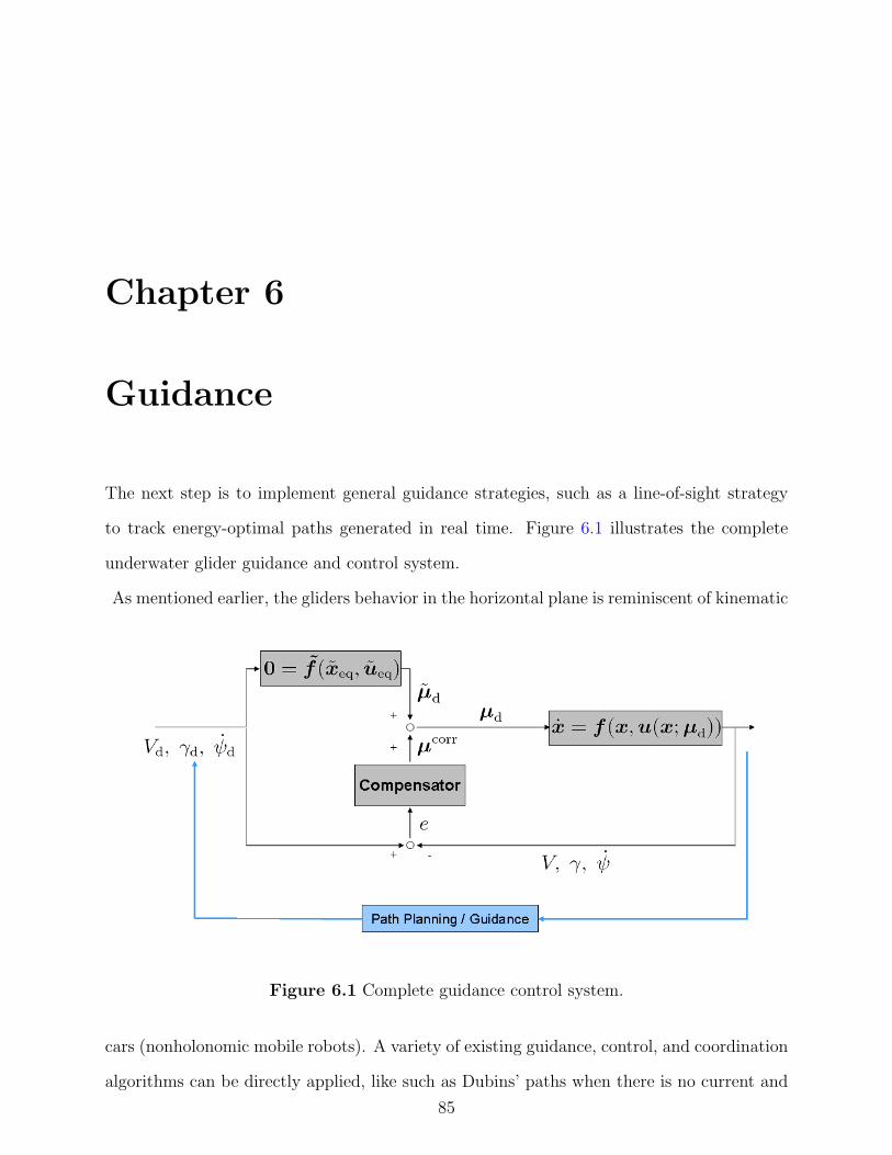
Chapter 6

Guidance

The next step is to implement general guidance strategies, such as a line-of-sight strategy

to track energy-optimal paths generated in real time. Figure 6.1 illustrates the complete

underwater glider guidance and control system.

As mentioned earlier, the gliders behavior in the horizontal plane is reminiscent of kinematic

Figure 6.1 Complete guidance control system.

cars (nonholonomic mobile robots). A variety of existing guidance, control, and coordination

algorithms can be directly applied, like such as Dubins’ paths when there is no current and

85

6.1 Path Planning 86

“convected” Dubins’ paths in the presence of uniform currents ( [45] and [46]). These Dubins-

like paths accommodate turn rate and turn acceleration limits, which are essential aspects of

underwater glider motion. For underwater gliders travelling at constant speed and maximum

flight efficiency, minimum arclength paths are minimum energy paths. Hence, energy-efficient

paths can be obtained by generating sequences of steady wings-level and turning motions.

This chapter illustrates tracking a Dubins path and the coordinated flight of two underwater

gliders [47].

6.1 Path Planning

A logical next step is to develop a procedure for optimal path planning which makes use

of the preceding approximate results for equilibrium turning flight. A reasonable objective

would be to concatenate these approximate equilibrium motions in order to minimize the

time of transit from a given initial point to a given final point with a specified initial and

final heading. The question of reachability naturally arises, since an underwater glider

must ascend or descend to locomote. A glider cannot progress between two points at the

same depth, for example, without concatenating at least one ascending and one descending

motion. For the moment, we will restrict our attention to situations in which the final point

is strictly below (or above) the initial point and can be reached in a single descending (or

ascending) flight without exceeding the vehicle’s physical limitations (such as the minimum

glide slope). More precisely, we will project the vehicle path onto the horizontal plane and

simply ignore the vertical component of motion. A fortunate consequence of the structure

of our approximate solution for turning flight is that, to first-order in ε, the horizontal

and vertical components of velocity remain constant. Thus, the minimum time problem in

the horizontal plane corresponds to minimizing the change in depth for a given horizontal

point-to-point transition. Since an underwater glider propels itself by the force of gravity,

minimizing the change in depth is equivalent to minimizing the energy expenditure.


To see that the horizontal component of velocity remains constant, to first order in ε,

recall that the speed V remains constant to first order in ε and note that

z = eT3 RIB(φ, θ, ψ)RBC(α, β) (V e1)

= eT3

(

ece3ψece2θece1φ)(

e−ce2αece3β)

(V e1)

= eT3

(

ece2(θ0)ece1(εφ1+O(ε2)))(

e−ce2(α0+O(ε2))ece3(εβ1+O(ε2))) (

(V0 +O(ε2))e1

)

= −V0 sin (θ0 − α0) +O(ε2).

Of course, −V0 sin (θ0 − α0) is precisely the vertical component of velocity in unperturbed,

wings level flight. An important consequence of this observation is that, since both the

magnitude and the vertical component of velocity remain constant, to first order in ε, so does

the horizontal component of velocity. Projecting the vehicle’s motion onto the horizontal

plane, glider equilibrium motions correspond to constant-speed straight-line and circular

paths. The speed is determined solely by the vehicle net weight and, in practice, may be

assumed to take the maximum achievable value. Considering only motion in the horizontal

plane, the control problem reduces to the following: choose the turn rate to minimize the

time of transit from a given initial point to a given final point with a specified initial and

final heading.

6.1.1 Dubins’ Car

Viewing the glider motion from directly above, the minimum time control problem is rem-

iniscent of Dubins’ car [45], a planar vehicle which drives forward at constant speed and

which may turn, in either direction, at any rate up to some maximum value. Dubins showed

that the minimum time control policy which brings the car from a given point to another,

with specified initial and final directions, is a concatenation of three motions: a left or right

turn at maximum rate, a straight transit or a second turn at maximum rate, and a final turn

at maximum rate. Note that a constant speed turn at maximum turn rate corresponds to a

turn of minimum radius. (Actually, Dubins considered the problem in terms of minimizing


the length of a continuous curve with limits on the curvature, but the two problems are

equivalent.) Variations of Dubins’ problem have enjoyed renewed attention in recent years,

in part because of increasing interest in mobile robotics. Reeds and Shepp [48] character-

ized the family of optimal trajectories for a variation of Dubins’ car in which the vehicle

could move in reverse, as well as forward. Sussmann and Tang [49] generalized further by

“convexifying” the non-convex control set defined in [48], managing to sharpen the results

presented by Reeds and Shepp and by Dubins. Parallel studies, as outlined in a series of

INRIA technical reports and papers [50–53], also investigated controllability and optimal

path planning for Dubins and Reeds-Shepp mobile robots. Anisi’s thesis [3] reviews some of

the recent results and provides some historical context.

For the purpose of explaining the Dubins’ car problem, let x = [x, y, ψ]T represent the

vehicle’s state (i.e., its position and heading in the horizontal plane) and let the turn rate

u = r be the input, which satisfies the inequality constraint |r| ≤ |rmax|. The vehicle moves

at some constant, nonzero forward speed V . Then the equations of motion are

x = f(x, u) where f(x, u) =

V cosψ

V sinψ

u

. (6.1)

Although Dubins’ problem was originally presented as one of minimizing the arclength of

a continuously differentiable curve, it may be re-stated as follows: Find an input history

which brings the system from a specified initial state x(0) = x0 to a specified final state

x(tf ) = xf while minimizing tf > 0. Note that, since the speed is constant, this minimum

time problem is equivalent to Dubins’ minimum arclength problem.

As shown in [45], the optimal history contains at most three distinct segments (i.e., two

switches of the control among its three possible values). These results are sharpened in [49],

where the control histories are shown to be of the type “BSB” (for “bang-singular-bang”) or

“BBB” (for “bang-bang-bang”). Having characterized the family of candidate optimal input

histories, it remains to actually choose the best one for a given initial and final state.


Figure 6.2 A geometric method for selecting the time-optimal path for Dubins’ carwhen the endpoints are more than twice the minimum turn radius apart [3].

Considering, for example, the case where the intermediate transit is a straight path that

is much longer than the vehicle turn radius, a simple, geometric algorithm as illustrated in

Figure 6.2 provides the optimal path. One defines two oriented circles of minimum radius

that are tangent to the initial velocity vector and two more oriented circles of minimum radius

that are tangent to the final velocity vector. Connecting the circles by directed tangents that

are consistent with the sense of the circles yields four admissible paths. Because the vehicle

moves at constant speed, the path of minimum arclength is the minimum time path.

To apply the approach described here to an underwater glider, assume that the glider is

executing some nominal gliding motion at a given glide slope and speed. Given an initial

heading, a desired final heading may be attained, at least approximately, by solving the

Dubins’ problem for the horizontal projected motion. Recall that the minimum time problem

in the horizontal plane corresponds to minimizing the change in depth, which equates to

minimizing the propulsive energy expenditure. This is an appealing feature of Dubins’

paths, given that underwater gliders are specifically designed for propulsive efficiency.

6.1.2 Dubins’ Car with Control Rate Limits

The classical Dubins’ car problem assumes that turn rate can be treated as an input with

magnitude limits but no rate limits. (Equivalently, the arclength minimization problem


Figure 6.3 Dubins’ paths: Constant speed; no current.

imposes limits on the curvature but not on its derivative.) The assumption may or may not

be appropriate for wheeled robotic vehicles, but it is certainly not appropriate for underwater

gliders. For these vehicles, turn rate is controlled indirectly by shifting the center of gravity to

effect a banked turn. To explore the effect of control rate limits on the Dubins optimal path

result, one may augment the state vector given in Section 6.1.1 as follows: x = [x, y, ψ, r]T .

Let the turn acceleration be the input u = r, where r satisfies the state inequality constraint

|r| ≤ |rmax| and u satisfies the input inequality constraint |u| ≤ |umax|. The equations of

motion are

x = f(x, u) where f(x, u) =

V cosψ

V sinψ

r

u

.

Although we now consider turn acceleration as an input, we still assume that the underwater

glider state varies in a quasi-steady manner. That is, we assume that the vehicle state varies

along the continuum of (approximate) equilibrium states, as parameterized by the turn rate.

Under this assumption, as shown in Section 3.2, the vehicle’s speed V remains constant to

first-order in the turn rate.

In fact, this problem has been treated in some detail by Scheuer [54], as summarized in


[43]. Her work extends that of Boissonnat and colleagues [55] and of Kostov and Degtiariova-

Kostova [56], who considered the case where the derivative of the turn rate (equivalently, the

derivative of curvature) is constrained, but not the magnitude of the turn rate. In [55], it was

shown that time-optimal paths exist and that they consist of straight segments and clothoids

at maximum turn acceleration. It was also shown that the minimum time curves can be quite

complicated, possibly including infinitely many clothoidal segments. Independently, Kostov

and Degtiariova-Kostova [56] proposed a method for constructing suboptimal paths from

clothoids and straight segments. The term “suboptimal,” as used in [56], means that the

amount by which the transit time exceeds the minimum time is bounded by a function of

the turn acceleration limit.

6.1.3 Dubins’ Car in the Presence of Currents

Ocean currents can also significantly influence a glider’s motion, even at depth. Because

underwater gliders move quite slowly, relative to conventional AUVs, and operate over much

longer time spans, even light currents can have a large, cumulative effect on vehicle motion.

The Dubins path planning procedure has recently been extended to the case of a constant

ambient current in [46, 57]. In the approach described in these papers, the Dubins path is

planned relative to the (moving) ambient fluid with suitably re-defined endpoint conditions.

In [46], authors provide a geometric method for generating candidate time-optimal paths

in steady wind by concatenating straight and trochoidal segments (see Figure 6.4). With

wind approaching from the west in Figure 6.4, there are two candidate extremals, shown

by blue curves, corresponding to trochoidal segments with clockwise and counter-clockwise

orientations, respectively. The path with shorter arc length is the one with shorter total

time requirement.

6.2 Guidance Strategies 92

Figure 6.4 Convected Dubins paths: Constant speed; uniform current.

6.2 Guidance Strategies

The goal here is to present examples of guidance strategies which use the previously developed

motion control system to make underwater gliders fly in a desired pattern. The desired

pattern is mission specific. We present two cases. First, we consider the energy-efficient

paths discussed in Section 6.1. Second, we consider the problem of forcing two or more

gliders to follow the same ground track at different depths. In Section 6.2.1 we describe

a trajectory tracking approach in the horizontal plane that has been described in [58]. In

Section 6.2.2 we describe a method for planar collective motion described in [59]. In both

cases, the authors assumed a kinematic car model. Here, we consider the actual dynamics

of the underwater glider and seek a desired turn rate ψd as in Figure 6.1.

6.2.1 Planar Trajectory Tracking

The aim is to drive the vehicle along a desired path with constant speed. We assume that we

have prior knowledge of the vehicle’s mission path and the path can be constructed of line

segments or segments with a constant curvature, such as Dubins’ paths. The path following

controller should eliminate both cross-track error (the distance from the vehicle to the path)

and heading error (the angle between the vehicle velocity and the tangent to the path) [60].

This motivates the development of the vehicle kinematic model in terms of path parameters


in a Serret-Frenet frame and the use of the cross track and heading error as coordinates of

the error space where the control problem will be formulated.

Following [58], consider a frame Fs along the desired path, with its x-axis in the direction

of the desired inertial velocity, i.e., tangential to the path, and its y-axis normal to the path.

Let s be the arclength along the desired path. With s indicating a position on the path, the

curvature κ(s) at that position is defined as κ(s) = 1/R(s), where R(s) is the radius of the

path at that point. If the direction of the path is indicated as ψs then the path parameters

are related to yaw-rate as ψs(s) = κ(s)s,

s

ys

˙ψ

=

cos(ψ)1−κys

0

sin ψ 0

−κ cos(ψ)1−κys

1

V0

ψd

where ψ = ψd − ψs, which is the difference between desired path and the vehicle’s heading.

The guidance objective is to force ψ and ys simultaneously to zero. This may be achieved

by constructing the commanded control signal (ψc(ys)) as a function of “cross-track error”

ys. A common logic is a pursuit-guidance law,

ψc(ys) = − arctan(ysd

)

where d is a constant “look-ahead” distance. Or the Helmsman logic can be used

ψc = ψicpt(e−

a2ys − 1)

(e−a2ys + 1)

˙ψc = −aψicpte−

a2ys

(e−a2ys + 1)2

V0 sin(ψ),

where a is Helmsman sensitivity parameter and ψicpt is the intercept heading [58].

The desired turn rate can be obtained from

˙ψd = −kd ˙ψ + kd0(˙ψc − ˙ψ) + kp(ψc − ψ) + νk.

One must choose kd, kd0 , and kp properly. A kinematics feedforward term νk = κV0 replaces

the need for integral action for constant-curvature path following.


Figures 6.6–6.10 illustrate the effectiveness of the described guidance method, together

with the motion control system developed in Chapter 4, when a Slocum glider tracks a

Dubins path.

6.2.2 Coordination on Helical Paths

In many environmental sampling problems, it is important to characterize the flux (direction

and magnitude) through a control volume boundary. Underwater gliders can follow a helical

path and collect ocean data in the desired control volume. Multiple gliders, working in

coordination, can enable or enhance this capability. For example, one application would

be measuring the flux of energy through sea-floor hydrothermal vents. This is important

to determine the nature of hydrothermal systems, as well as their role in the oceans and,

more generally, the Earth’s ecosystem [61]. Underwater gliders can measure the ocean’s

vertical temperature independently while flying in coordination at different depths. This is

necessary to account for the fact that turbulent mixing does not occur uniformly over the

entire ocean [7].

Following the algorithm presented in [59], we consider each glider moving in constant

speed V0 subject to steering control uk. Choosing the control law for glider k ∈ {1, . . . , N},

uk = uk1 + uk2 ,

enforces motion of all gliders in the same direction in synchronization, where uk1 guarantees

the convergence on the circle and uk2 gives the desired phase arrangement. For parallel

formation on a cylinder with radius R0, they are defined as

uk1 = −Kc

N

N∑

j=1

sin(ψj − ψk)

uk2 = ω0(1 + κcR0V0 cos(ψk − ϑk))

where ϑk = arctan( ykxk

). One can choose control gains Kc and κc properly. Then, the desired

turn rate can be obtained from ψkd = uk.


Figures 6.11–6.15 illustrate the effectiveness of this guidance method, together with the

motion control system developed in Chapter 4, when two Slocum gliders fly in coordination

on a helical path.

−50−40

−30−20

−100

1020

3040

50

0 10 20 30 40 50 60 70 80 90 100 110 120 130 140 150 159

0

10

20

30

40

50

x (m)

y(m)

z (m

)

Figure 6.5 Slocum trajectory in 3D following a Dubins path.


We present simulation results for two cases: first a Slocum tracks a commanded Dubins path,

and then two Slocum gliders perform coordinated flight on a helical path. We consider the

flight condition and PID control parameters presented in Section 4.5 to obtain the results.

Figure 6.5 shows the result of planar path following of Slocum in 3D, considering the

following values for the servo-actuator parameters

ωnx= 20 rad/s, ζx = 0.001, and ζrx= 1

ωny= 20 rad/s, ζy = 0.01, and ζry= 1

with ωrx = ωry = 1 rad/s, which means we are not considering the actuators’ rate limit in

this case. The guidance law parameters are a = 2, ψicpt = π/4, kp = 10, kd = 1, kd0 = 0, and

νk = 0. Figure 6.6 illustrates the effectiveness of the guidance control system in following a


0 20 40 60 80 100 120 140 160−60

−40

−20

0

20

40

60

y (m)

x (m

)

Slocum pathDubins path

Figure 6.6 Slocum following a Dubins path.

desired Dubins path. Figure 6.7 shows the lateral mass location in response to a command

sequence that is intended to effect a right turn, a straight segment, and left turn (viewed

from above) from an initial point to a desired final point. The heading rate ψd is directly

commanded as shown in Figure 6.8, with the lateral moving mass actuator responding as

necessary. Figure 6.9 illustrates the location of the longitudinal moving mass, which must

move in order to regulate the glide path angle shown in Figure 6.10.

Figure 6.11 illustrates glide synchronization of two Slocum gliders on a helical path, where

Glider 1 starts at (x1(0), y1(0), z1(0)) = (5, 5, 25) and Glider 2 starts at (x2(0), y2(0), z2(0)) =

(−5,−5, 0). For this case, we consider ωrx = ωry = 0.8 rad/s for both gliders. The guidance

parameters are Kc = −0.01 and κc = 0.04.

Figure 6.12 shows the variation of the position of the lateral moving mass of two gliders

while coordinating to achieve the desired turn rate. Figure 6.13 illustrates time history of

turn rate to reach 0.025 rad/s and perform a synchronized flight on a circle with radius of

27.5 m. The time history of the position of the longitudinal moving mass of the two gliders


0 50 100 150 200 250

−0.15

−0.1

−0.05

0

0.05

0.1

0.15

t (s)

Late

ral M

ovin

g M

ass

Loca

tion

(m)

rp

y

rp

yd

Figure 6.7 Lateral moving mass location.

to maintain the nominal flight path angle is shown in Figure 6.14. See Figure 6.15 for the

time history of the flight path angle.


0 50 100 150 200 250 300−0.04

−0.03

−0.02

−0.01

0

0.01

0.02

0.03

0.04

t (s)

r (r

ad/s

)

rrd

Figure 6.8 Turn rate response following Dubins’ path.

0 50 100 150 200 250

−0.015

−0.01

−0.005

0

0.005

0.01

0.015

t (s)

Long

itudi

nal M

ovin

g M

ass

Loca

tion

(m)

rp

x

rp

xd

Figure 6.9 Longitudinal moving mass position.


0 50 100 150 200 250−14.5

−14

−13.5

−13

−12.5

−12

−11.5

t (s)

Flig

ht p

ath

angl

e (°

)

γγd

Figure 6.10 Glide path angle response following Dubins’ path.

−30 −20 −10 0 10 20 30 40

−30

−20

−10

0

10

20

30

40

50

x (m)

y (m

)

Glider 1Glider 2

Figure 6.11 Synchronization of two Slocum gliders for control volume sampling.


0 100 200 300 400 500 600 700 8000

0.05

0.1

0.15

0.2

0.25

t (s)

Late

ral M

ovin

g M

ass

Loca

tion

(m)

rp

y1

rp

y2

Figure 6.12 Position of lateral moving mass.

0 100 200 300 400 500 600 700 800−0.005

0

0.005

0.01

0.015

0.02

0.025

0.03

0.035

0.04

t (s)

Tur

n ra

te (

rad/

s)

r1

r2

Figure 6.13 Slocum gliders’ turn rate.


0 50 100 150 200 250 300 350

−0.015

−0.01

−0.005

0

0.005

0.01

0.015

t (s)

Long

itudi

nal M

ovin

g M

ass

Loca

tion

(m)

rp

x1

rp

x2

Figure 6.14 Position of longitudinal moving mass.

0 100 200 300 400 500 600 700 800

−13.2

−13

−12.8

−12.6

−12.4

−12.2

−12

−11.8

−11.6

t (s)

Flig

ht p

ath

angl

e (°

)

γ1

γ2

Figure 6.15 Slocum gliders’ glide path angle.

Chapter 7

Conclusions and Future Work

An approximate solution for steady turning motions of underwater gliders has been derived

using a sophisticated dynamic model. The problem was formulated as a regular perturbation

problem using wings-level, equilibrium flight as the nominal state and turn rate as the small

perturbation parameter. As an illustration, the result was applied to an existing model of the

Slocum underwater glider. The analytical result, though approximate, is valuable because it

gives better insight into the effect of parameters on vehicle motion and stability. This insight

can, in turn, lead to better usage guidelines for current vehicles and design guidelines (e.g.,

actuator sizing) for future vehicles.

Building on results in glider steady motion analysis, a feedforward/feedback motion con-

trol system was presented to control speed, glide path angle, and turn rate. The control sys-

tem uses feedforward commands obtained from an approximate solution for steady turning

motion and includes feedback to compensate for approximation error and other uncertain-

ties. The control system design includes model reference controllers for the servo-actuators,

to allow actuator rate and magnitude saturation effects to be more easily analyzed and ac-

commodated. Stability of the closed-loop system was analyzed using slowly varying systems

theory in which the turn rate command was treated as a slowly varying parameter. A bound

on turn acceleration was obtained as a product of the analysis. The controller’s effectiveness

102

103

was demonstrated in a simulation of a multi-body model of the underwater glider Slocum.

The proposed control system provides a mechanism for path following. The next step

was to implement a guidance strategy, together with a path planning strategy, and one

which continues to exploit the natural efficiency of this class of vehicle. The structure of

the approximate solution for steady turning motion is such that, to first order in turn rate,

the glider’s horizontal component of motion matches that of “Dubins’ car,” a kinematic

car with bounded turn rates. Dubins’ car is a classic example in the study of time-optimal

control for mobile robots. For an underwater glider, one can relate time optimality to energy

optimality. Specifically, for an underwater glider travelling at a constant speed and maximum

flight efficiency (i.e., maximum lift-to-drag ratio), minimum time paths are minimum energy

paths. Hence, energy-efficient paths can be obtained by generating sequences of steady

wings-level and turning motions. These efficient paths can, in turn, be followed using the

motion control system described here. A variety of guidance and path planning algorithms

can be directly applied. The motion control system is applied to tracking of a Dubins path

and coordination on a helical path.

An obvious next step is physical implementation of the proposed feedforward/feedback

motion controller on an underwater glider. Virginia Tech and University of Washington

are currently collaborating to implement the developed controller on Seaglider. Ongoing

analysis focuses on tracking suboptimal Dubins paths which accommodate turn rate and

turn acceleration limits in the presence of uniform currents.

Bibliography

[1] Geisbert, J. S., Hydrodynamic Modeling for Autonomous Underwater Vehicles Using

Computational and Semi-Empirical Methods , Master’s thesis, Virginia Polytechnic In-

stitute & State University, Blacksburg, VA, June 2007.

[2] Stengel, R. F., Flight Dynamics , Princeton University Press, Princeton, NJ, 2004.

[3] Anisi, D. A., “Optimal motion control of a ground vehicle,” Tech. Rep. FOI-R–0961–SE,

Swedish Defence Research Agency, Stockholm, Sweden, July 2003.

[4] “AUV Technologies,” Autonomous Undersea Vehicle Applications Center Website, Au-

gust 2009, Available at http://auvac.org/resources/.

[5] Woithe, H. C., Tilkijieva, D., and Kremer, U., “Toward a Resuorce-Aware Programming

Architecture for Smart Autonomous Underwater Vehicles,” Technical Report DCS-TR-

637, Rutgers University, June 2008.

[6] Leonard, N. E., Paley, D. A., Lekien, F., Sepulchre, R., Fratantoni, D. M., and Davis,

R. E., “Collective Motion, Sensor Networks, and Ocean Sampling,” Proceedings of the

IEEE , Vol. 95, No. 1, January 2007, pp. 48–74.

[7] Tropea, C., Yarin, A. L., and Foss, J. F., editors, Springer Handbook of Experimental

Fluid Mechanics , Springer, 2007.

[8] Stommel, H., “The Slocum mission,” Oceanography , Vol. 2, 1989, pp. 22–25.

104

BIBLIOGRAPHY 105

[9] Graver, J. G., Underwater Gliders: Dynamics, Control, and Design, Ph.D. thesis,

Princeton University, 2005.

[10] Webb, D. C., Simonetti, P. J., and Jones, C. P., “SLOCUM: An Underwater Glider

Propelled by Environmental Energy,” Journal of Oceanic Engineering , Vol. 26, No. 4,

2001, pp. 447–452, Special Issue on Autonomous Ocean-Sampling Networks.

[11] Eriksen, C. C., Osse, T. J., Light, R. D., Wen, T., Lehman, T. W., Sabin, P. L., Ballard,

J. W., and Chiodi, A. M., “Seaglider: A Long-Range Autonomous Underwater Vehicle

for Oceanographic Research,” Journal of Oceanic Engineering , Vol. 26, No. 4, 2001,

pp. 424–436, Special Issue on Autonomous Ocean-Sampling Networks.

[12] Sherman, J., Davis, R. E., Owens, W. B., and Valdes, J., “The Autonomous Underwater

Glider “Spray”,” Journal of Oceanic Engineering , Vol. 26, No. 4, 2001, pp. 437–446,

Special Issue on Autonomous Ocean-Sampling Networks.

[13] Davis, R. E., Eriksen, C. C., and Jones, C. P., “Autonomous Buoyancy-Driven Un-

derwater Gliders,” Technology and Applications of Autonomous Underwater Vehicles ,

edited by G. Griffiths, Vol. 2, chap. 3, Taylor and Francis, 2002.

[14] Jenkins, S. A., Humphreys, D. E., Sherman, J., Osse, J., Jones, C., Leonard, N., Graver,

J., Bachmayer, R., Clem, T., Carroll, P., Davis, P., Berry, J., Worley, P., and Wasyl, J.,

“Underwater Glider System Study,” Tech. Rep. 53, Scripps Institution of Oceanography,

May 2003.

[15] Jones, C., Webb, D., Glenn, S., Schofield, O., Kerfoot, J., Kohut, J., Roarty, H., Aragon,

D., Haldeman, C., Haskin, T., and Kahl, A., “Slocum Glider Extending the Endurance,”

The 16th International Symposium on Unmanned Untethered Submersible Technology

(UUST09), Durham, NH, August 23-26 2009.

[16] Mientka, M., “Gliders Flying onto the World’s Scientific Stage More Improvements

Planned,” Unmanned Systems , Vol. 27, No. 1, January 2009, pp. 22 – 23.

BIBLIOGRAPHY 106

[17] Hines, S., “Seaglider monitors waters from Arctic during record-

breaking journey under ice,” EurekAlert , April 28 2009, Available at

http://www.eurekalert.org/pub-releases/2009-04/uow-smw042809.php.

[18] “iRobot Seaglider,” iRobot Corporation Website, September 2009, Available at

http://www.irobot.com/sp.cfm?pageid=393.

[19] Tomoda, Y., Kawaguchi, K., Ura, T., and Kobayashi, H., “Development and Sea Tri-

als of a Shuttle Type AUV “ALBAC”,” In Proc. 8th Int. Symposium on Unmanned

Untethered Submersible Tech., 1993.

[20] Guo, C. and Kato, N., “Mini Underwater Glider (MUG) for Education,” Workshop for

Asian and Pacific Universities’ Underwater Roboticians (APuuRobo 2008), Institute of

Industrial Science, The University of Tokyo, Japan, January 2008.

[21] Graver, J. G., Liu, J., Woolsey, C. A., and Leonard, N. E., “Design and Analysis of

an Underwater Glider for Controlled Gliding,” Conference on Information Sciences and

Systems , 1998, pp. 801–806.

[22] Scott, R. D., Cooperative Tracking for Persistent Littoral Undersea Surveillance, Mas-

ter’s thesis, Massachusetts Institute of Technology, June 2007.

[23] Rusling, M., “Gliders Will Aid Naval Research,” National Defense Indus-

trial Association Business and Technology Magazine, June 2009, Available at

http://www.nationaldefensemagazine.org/archive/2009/June/Pages/.

[24] GmbH, E., “Lessons learned from fish fins,” 2008, Available at

http://www.evologics.de/en/products/.

[25] Godin, M. and Fulton-Bennett, K., “Monterey Bay 2006 field experi-

ments,” Montray Bay Aquarium Research Institute, August 2006, Available at

http://www.mbari.org/MB2006/UPS/mb2006-ups-links.htm.

BIBLIOGRAPHY 107

[26] Bhatta, P., Nonlinear Stability and Control of Gliding Vehicles, Ph.D. thesis, Princeton

University, 2006.

[27] Leonard, N. E. and Graver, J. G., “Model-Based Feedback Control of Autonomous

Underwater Gliders,” Journal of Oceanic Engineering , Vol. 26, No. 4, 2001, pp. 633–

645, Special Issue on Autonomous Ocean-Sampling Networks.

[28] Galea, A. M., Optimal path planning and high level control of an autonomous gliding

underwater vehicle, Master’s thesis, Massachusetts Institute of Technology, 1999.

[29] Bachmayer, R., Graver, J., and Leonard, N. E., “Glider Control: A Close Look into the

Current Glider Controller Structure and Future Developments,” IEEE Oceans 2003 ,

Vol. 2, 2003, pp. 951–954.

[30] Woolsey, C. A., “Reduced Hamiltonian Dynamics for a Rigid Body/Mass Particle Sys-

tem,” Journal of Guidance, Control, and Dynamics , Vol. 28, No. 1, January-February

2005, pp. 131–138.

[31] Mahmoudian, N., Geisbert, J., and Woolsey, C. A., “Dynamics & Control of Un-

derwater Gliders I: Steady Motions,” Tech. Rep. VaCAS-2007-01, Virginia Center

for Autonomous Systems, Virginia Tech, Blacksburg, VA, June 2007, Available at

http://www.unmanned.vt.edu/discovery/reports.html.

[32] Mahmoudian, N., Woolsey, C., and Geisbert, J., “Steady Turns and Optimal Path for

Underwater Gliders,” AIAA Guidance, Navigation and Control Conference and Exhibit,

Hilton Head, SC, Aug 20-23 2007.

[33] Mahmoudian, N. and Woolsey, C. A., “Underwater glider motion control,” IEEE Con-

ference on Decision and Control , Cancun, Mexico, December 2008, pp. 552 – 557.

[34] Fossen, T. I., Guidance and Control of Ocean Vehicles , John Wiley and Sons, 1995.

BIBLIOGRAPHY 108

[35] Stevens, B. L. and Lewis, F. L., Aircraft control and simulation, Second Ed., John Wiley

and Sons, INC., Hoboken, N.J., 2003.

[36] Etkin, B. and Reid, L., Dynamics of Flight Stability and Control , John Wiley and

Sons,Inc., New York, 1996.

[37] Guckenheimer, J. and Holmes, P., Nonlinear Oscillations, Dynamical Systems, and

Bifurcations of Vector Fields , Springer-Verlag, New York, NY, 1983.

[38] Hartman, P., Ordinary Differential Equations , John Wiley and Sons, Inc., New York,

NY, 1964.

[39] Mahmoudian, N. and Woolsey, C., “Analysis of Feedforward/Feedback Control Design

for Underwater Gliders Based on Slowly Varying Systems Theory,” AIAA Guidance,

Navigation and Control Conference and Exhibit, Chicago, IL, Aug 20-23 2009.

[40] Khalil, H. K., Nonlinear Systems , Prentice Hall, Upper Saddle River, NJ, 3rd ed., 2002.

[41] Rugh, W. J., Linear System Theory , Prentice Hall, Upper Saddle River, NJ, 2nd ed.,

1996.

[42] Kostov, V. and Degtiariova-Kostova, E., “Suboptimal paths in the problem of a planar

motion with bounded derivative of the curvature,” Tech. Rep. 2051, Institut National

de Recherche en Informatique et en Automatique (INRIA), July 1993.

[43] Scheuer, A. and Laugier, C., “Planning sub-optimal and continuous-curvature paths

for car-like robots,” IEEE/RSJ International Conference on Intelligent Robots and Sys-

tems , Victoria, B.C., Canada, October 1998, pp. 25–31.

[44] Mahmoudian, N. and Woolsey, C., “Feedforward/Feedback Tracking of a First Or-

der Approximate Equilibrium Manifold,” American Mathematical Society 2009 Spring

Southeastern Meeting, Raleigh, NC, April 4-5 2009.

BIBLIOGRAPHY 109

[45] Dubins, L. E., “On curves of minimal length with a constraint on average curvature

and with prescribed initial and terminal positions and tangents,” American Journal of

Mathematics , Vol. 79, 1957.

[46] Techy, L., Woolsey, C. A., and D. G. Schmale, I., “Path planning for efficient UAV

coordination in aerobiological sampling missions,” IEEE Conference on Decision and

Control , Cancun, Mexico, December 2008, pp. 2814–2819.

[47] Mahmoudian, N. and Woolsey, C., “Efficient Guidance and Control for Underwater

Gliders,” The 16th International Symposium on Unmanned Untethered Submersible

Technology (UUST09), Durham, NH, August 23-26 2009.

[48] Reeds, J. A. and Shepp, L. A., “Optimal paths for a car that goes both forwards and

backwards,” Pacific Journal of Mathematics , Vol. 145, No. 2, 1990, pp. 367–393.

[49] Sussmann, H. J. and Tang, G., “Shortest paths for the Reeds-Shepp car: A worked out

example of the use of geometric techniques in nonlinear optimal control,” Tech. Rep.

91-10, Rutgers University Center for Systems and Control, New Brunswick, NJ, 1991.

[50] Boissonnat, J.-D., Cerezo, A., and Leblond, J., “Shortest paths of bounded curvature in

the plane,” IEEE International Conference on Robotics and Automation, Nice, France,

May 1992, pp. 2315–2320.

[51] Soueres, P., Fourquet, J.-Y., and Laumond, J.-P., “Set of reachable positions for a car,”

IEEE Transactions on Automatic Control , Vol. 39, No. 8, August 1994, pp. 1626–1630.

[52] Bui, J.-D. B. X.-N., “Accessibility region for a car that only moves forwards along

optimal paths,” Tech. Rep. 2181, Institut National de Recherche en Informatique et en

Automatique (INRIA), January 1994.

BIBLIOGRAPHY 110

[53] Bui, X.-N., Boissonnat, J.-D., Soueres, P., and Laumond, J.-P., “Shortest path syn-

thesis for Dubins Non-holomic robot,” IEEE International Conference on Robotics and

Automation, San Diego, CA, May 1994.

[54] Scheuer, A., Planification de chemin a courbure continue pour robot mobile non-

holonome, Ph.D. thesis, Institut National Polytechnique de Grenoble, 1998.

[55] Boissonnat, J.-D., Cerezo, A., and Leblond, J., “A note on shortest paths in the plane

subject to a constraint on the derivative of the curvature,” Tech. Rep. 2160, Institut

National de Recherche en Informatique et en Automatique (INRIA), January 1994.

[56] Kostov, V. and Degtiariova-Kostova, E., “The planar motion with bounded deriva-

tive of the curvature and its suboptimal paths,” Tech. Rep. 2189, Institut National de

Recherche en Informatique et en Automatique (INRIA), January 1994.

[57] McGee, T. G. and Hedrick, J. K., “Optimal path planning with a kinematic airplane

model,” Journal of Guidance, Control, and Dynamics , Vol. 30, No. 2, 2007, pp. 629–633.

[58] Rysdyk, R., “Unmanned Aerial Vehicle Path Following for Target Observation in Wind,”

Journal of Guidance, Control, and dynamics , Vol. 29, No. 5, 2006, pp. 1092–1100.

[59] Sepulchre, R., Paley, D. A., and Leonard, N. E., “Stabilization of Planar Collective

Motion: All-to-All Communication,” IEEE Transactions on Automatic Control , Vol. 52,

No. 5, 2007, pp. 811–824.

[60] Encarnacao, P. and Pascoal, A., “3D Path Following for Autonomous Underwater Ve-

hicle,” 39th IEEE Conference on Decision and Control, Sydney, Australia, December

2000.

[61] Veirs, S. R., Heat flux and hydrography at a submarine volcano: Observations and models

of the Main Endeavour vent field in the northeast Pacific, Ph.D. thesis, University of

Washington, 2003.

eï¬ƒcient motion planning and control for underwater gliders

Documents