http://www.ee.unlv.edu/~b1morris/ecg782/

Professor Brendan Morris, SEB 3216, brendan.morris@unlv.edu

ECG782: Multidimensional

Digital Signal Processing

Spring 2014

TTh 14:30-15:45 CBC C313

Lecture 05

Image Processing Basics

13/02/04

Outline

• Linear Systems

• 1D Fourier Review

• 2D Fourier Transform

• Discrete Cosine Transform

• Wavelet Transform

2

Linearity

• Image processing as a system

• Linearity defined on vector (linear) spaces ▫ Superposition principle:

Additivity Homogeneity

▫ ℒ 𝑎𝑥1 + 𝑏𝑥2 = 𝑎ℒ 𝑥1 + 𝑏ℒ(𝑥2)

• Very important property for linear image processing ▫ Can make use of 1D signal processing ideas

3

ℒ 𝑥 𝑦

Dirac Delta Distribution

• Dirac delta - 𝛿 𝑥, 𝑦

▫ Impulse - 𝛿 𝑥, 𝑦 = 0 ∀ 𝑥, 𝑦 ≠ 0

▫ 𝛿 𝑥, 𝑦 𝑑𝑥𝑑𝑦 = 1∞

−∞

∞

−∞

• Sifting property

▫ Use of 𝛿 𝑥, 𝑦 to obtain value of function

▫ 𝑓 𝑥, 𝑦 𝛿(𝑥 − 𝜆, 𝑦 − 𝜇)𝑑𝑥𝑑𝑦 = 𝑓(𝜆, 𝜇)∞

−∞

∞

−∞

• Delta sampling

▫ 𝑓 𝑎, 𝑏 𝛿(𝑎 − 𝑥, 𝑏 − 𝑦)𝑑𝑎𝑑𝑏 = 𝑓(𝑥, 𝑦)∞

−∞

∞

−∞

4

Convolution • In image processing, this is an

“overlap” operation • 1D convolution

▫ 𝑓 ∗ ℎ 𝑡 =

𝑓 𝜏 ℎ 𝑡 − 𝜏 𝑑𝜏∞

−∞=

ℎ 𝜏 𝑓 𝑡 − 𝜏 𝑑𝜏∞

−∞

▫ Limits restricted to finite support (similar to image range)

• Properties

▫ 𝑓 ∗ ℎ = ℎ ∗ 𝑓

▫ 𝑓 ∗ 𝑔 ∗ ℎ = 𝑓 ∗ 𝑔 ∗ ℎ

▫ 𝑓 ∗ 𝑔 + ℎ = 𝑓 ∗ 𝑔 + 𝑓 ∗ ℎ

▫ 𝑎 𝑓 ∗ 𝑔 = 𝑎𝑓 ∗ 𝑔 = 𝑓 ∗ (𝑎𝑔)

▫𝑑

𝑑𝑥𝑓 ∗ ℎ =

𝑑𝑓

𝑑𝑥∗ ℎ = 𝑓 ∗

𝑑ℎ

𝑑𝑥

• 2D convolution • 𝑓 ∗ ℎ 𝑥, 𝑦 =

𝑓 𝑎, 𝑏 ℎ(𝑥 − 𝑎, 𝑦 − 𝑏)𝑑𝑎𝑑𝑏∞

−∞

∞

−∞

• =

ℎ 𝑎, 𝑏 𝑓(𝑥 − 𝑎, 𝑦 − 𝑏)𝑑𝑎𝑑𝑏∞

−∞

∞

−∞

• = ℎ ∗ 𝑓 𝑥, 𝑦

• Discrete 2D convolution ▫ Linear preprocessing step ▫ Output pixel is a linear

combination of neighborhood pixels

• 𝑔 𝑖, 𝑗 = ℎ 𝑖 − 𝑚, 𝑗 − 𝑛 𝑓(𝑚, 𝑛)𝑚,𝑛 ∈𝒪

▫ 𝒪 – neighborhood (typically rectangular with odd number or rows and columns

▫ ℎ - kernel or convolution mask

5

Images as Linear Systems

• Image viewed as superposition of deltas

• 𝑔 𝑥, 𝑦 = 𝑓 𝑎, 𝑏 ℒ{𝛿 𝑎 − 𝑥, 𝑏 − 𝑦 }𝑑𝑎𝑑𝑏∞

−∞

∞

−∞

• 𝑔 𝑥, 𝑦 = 𝑓 𝑎, 𝑏 ℎ 𝑎 − 𝑥, 𝑏 − 𝑦 𝑑𝑎𝑑𝑏∞

−∞

∞

−∞

• 𝑔 𝑥, 𝑦 = (𝑓 ∗ ℎ)(𝑥, 𝑦) • Fourier transform relationship

• 𝐺 𝑢, 𝑣 = 𝐹 𝑢, 𝑣 𝐻(𝑢, 𝑣) ▫ Useful for frequency domain smoothing and

sharpening

6

ℒ 𝑓(𝑥, 𝑦) 𝑔(𝑥, 𝑦)

Intro Linear Integral Transforms

• Represent signals (images) in a more suitable domain ▫ Information is better “visible” ▫ Solution to related (dual) problem is easier

• Most often interested in the “frequency domain” ▫ What a one-to-one mapping between spatial

(image coordinates) and frequency Inverse transform must exist

▫ Popular transforms include: Fourier, Cosine, Wavelet

• Most often used for filtering ▫ Image-to-image mapping

7

1D Fourier Transform • 𝐹 𝑓 𝑡 = 𝐹 𝜉 =

𝑓 𝑡 𝑒−2𝜋𝑖𝜉𝑡𝑑𝑡∞

−∞

• Inverse transform ▫ 𝐹−1 𝐹 𝜉 = 𝑓 𝑡 =

𝐹 𝜉 𝑒2𝜋𝑖𝜉𝑡𝑑𝜉∞

−∞

• This always exists for digital signals (of finite length, e.g. images)

• Notice the FT is a linear combination of complex exponentials ▫ Linear combination of sines

and cosines

▫ 𝑒𝑗𝜃 = cos 𝜃 + 𝑗 sin 𝜃

▫ 𝐹(𝜉) – indicates the contribution of sinusoid with frequency 𝜉

8

1D Fourier Transform Representation

• In general, FT is complex valued

• Can express in polar form

▫ 𝐹 𝜉 = 𝐹 𝜉 𝑒−𝑖𝜙(𝜉)

• Magnitude spectrum

▫ 𝐹 𝜉 = 𝑅𝑒2(𝐹) + 𝐼𝑚2(𝐹) 1/2

• Phase spectrum (angle)

▫ 𝜙 𝜉 = tan−1 𝐼𝑚 𝐹

𝑅𝑒 𝐹

• Power spectrum

▫ 𝑃 𝜉 = 𝐹 𝜉 2 = 𝑅𝑒2(𝐹) + 𝐼𝑚2(𝐹)

9

Fourier Transform Properties • DC value (offset)

▫ 𝐹 0 = 𝑓 𝑡 𝑑𝑡∞

−∞

▫ Area under 𝑓(𝑡)

▫ Average value

• FT offset

▫ 𝑓 0 = 𝐹 𝜉 𝑑𝜉∞

−∞

• Parseval’s Theorem

▫ 𝑓 𝑡 2𝑑𝑡∞

−∞= 𝐹 𝜉 2𝑑𝜉

∞

−∞

▫ Energy in time domain is equal to energy in frequency domain

• Uncertainty principle ▫ Wide in time narrow in

frequency

▫ Narrow in time wide in frequency

10

Short Time Fourier Transform

• Non-stationary signal processing technique

▫ Signal distribution changes in time

• Divide signal into smaller pieces and do computations in windows

▫ Typically, smooth windows are selected to reduce border effects

• This gives a sense of “global” properties but also a time when they happen (which window)

▫ Global – mean, variance, frequency content

▫ Timing – which window

11

Discrete Fourier Transform

• Assume discrete signal obtained by sampling

▫ 𝑓 𝑛 , 𝑛 = 0…𝑁 − 1

• DFT

▫ 𝐹 𝑘 =1

𝑁 𝑓 𝑛 exp (−2𝜋𝑖

𝑛𝑘

𝑁)𝑁−1

𝑛=0

▫ 𝑓 𝑛 = 𝐹 𝑘 exp (2𝜋𝑖𝑛𝑘

𝑁)𝑁−1

𝑘=0

• Since DFT is discrete, it is periodic ▫ 𝑘 – represents a discrete frequency

• Fast Fourier transform (FFT) ▫ Fast implementation of DFT (𝑂(𝑛 log 𝑛)) ▫ Basic DFT is 𝑂 𝑛2 ▫ Makes frequency domain processing possible

12

2D Fourier Transform • Generalization of 1D FT

• 𝐹 𝑢, 𝑣 =

𝑓 𝑥, 𝑦 𝑒−2𝜋𝑖 𝑥𝑢+𝑦𝑣∞

−∞𝑑𝑥𝑑𝑦

∞

−∞

• 𝑓 𝑥, 𝑦 =

𝐹 𝑢, 𝑣 𝑒2𝜋𝑖 𝑥𝑢+𝑦𝑣∞

−∞𝑑𝑢𝑑𝑣

∞

−∞

• For images (𝑢, 𝑣) are called spatial frequencies ▫ FT indicates how to combine 2D

spatial sinusoids

• Properties:

• Linearity

▫ 𝐹 𝑎𝑓1 𝑥, 𝑦 + 𝑏𝑓2 𝑥, 𝑦 =𝑎𝐹1 𝑢, 𝑣 + 𝑏𝐹2 𝑢, 𝑣

• Time (spatial) shift

▫ 𝐹 𝑓 𝑥 − 𝑎, 𝑦 − 𝑏 =

𝐹 𝑢, 𝑣 𝑒−2𝜋𝑖 𝑎𝑢+𝑏𝑣

• Frequency shift

▫ 𝐹 𝑓 𝑥, 𝑦 𝑒2𝜋𝑖 𝑢0𝑥+𝑣0𝑦 =

𝐹 𝑢 − 𝑢0, 𝑣 − 𝑣0

• Real 𝑓(𝑥, 𝑦)

▫ 𝐹 −𝑢,−𝑣 = 𝐹∗(𝑢, 𝑣)

▫ Only need first quadrant for images (𝑢 ≥ 0, 𝑣 ≥ 0)

• Convolution duality

▫ 𝐹 𝑓 ∗ ℎ 𝑥, 𝑦 = 𝐹 𝑢, 𝑣 𝐻 𝑢, 𝑣

▫ 𝐹 𝑓 𝑥, 𝑦 ℎ 𝑥, 𝑦 = (𝐹 ∗ 𝐻)(𝑢, 𝑣)

13

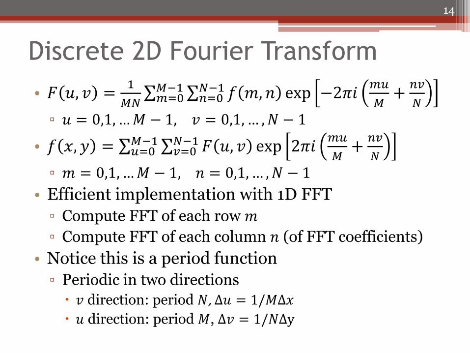
Discrete 2D Fourier Transform

• 𝐹 𝑢, 𝑣 =1

𝑀𝑁 𝑓 𝑚, 𝑛 exp −2𝜋𝑖

𝑚𝑢

𝑀+

𝑛𝑣

𝑁𝑁−1𝑛=0

𝑀−1𝑚=0

▫ 𝑢 = 0,1,…𝑀 − 1, 𝑣 = 0,1,… ,𝑁 − 1

• 𝑓 𝑥, 𝑦 = 𝐹 𝑢, 𝑣 exp 2𝜋𝑖𝑚𝑢

𝑀+

𝑛𝑣

𝑁𝑁−1𝑣=0

𝑀−1𝑢=0

▫ 𝑚 = 0,1,…𝑀 − 1, 𝑛 = 0,1,… ,𝑁 − 1

• Efficient implementation with 1D FFT

▫ Compute FFT of each row 𝑚

▫ Compute FFT of each column 𝑛 (of FFT coefficients)

• Notice this is a period function

▫ Periodic in two directions

𝑣 direction: period 𝑁, Δ𝑢 = 1/𝑀Δ𝑥

𝑢 direction: period 𝑀, Δ𝑣 = 1/𝑁Δy

14

2D Fourier Transform Example • Input image

▫ Assumed periodicity for harmonic frequencies (discrete)

• Remember that origin is typically in the top right

▫ Low frequency components are in the corners of FT image

15

More Fourier Transform Examples

16

More Fourier Transform Examples

• Higher values for edges and changing textures

▫ Notice the 45 degree line

• Importance of magnitude and phase

17

Sampling

• Sample the continuous image function

• Sampling function

▫ 𝑠 𝑥, 𝑦 = 𝛿(𝑥 − 𝑗Δ𝑥, 𝑦 − 𝑘Δ𝑦)𝑁𝑘=1

𝑀𝑗=1

Δ𝑥, Δ𝑦 – sampling intervals

• Sampling signal

• 𝑓𝑠 𝑥, 𝑦 = 𝑓 𝑥, 𝑦 𝑠 𝑥, 𝑦

▫ = 𝑓(𝑥, 𝑦) 𝛿(𝑥 − 𝑗Δ𝑥, 𝑦 − 𝑘Δ𝑦)𝑁𝑘=1

𝑀𝑗=1

• Taking FT of both sides

▫ 𝐹𝑠 𝑢, 𝑣 =1

Δ𝑥Δ𝑦 𝐹(𝑢 −

𝑚

Δ𝑥, 𝑣 −

𝑛

Δy)∞

𝑛=−∞∞𝑚=−∞

▫ Repeated copies of 𝐹(𝑢, 𝑣) (DTFT)

18

Shannon’s Sampling Theorem • Periodic copies of spectrum can

result in image distortion (aliasing)

▫ Occurs when copies overlap

▫ Caused by undersampling

• Shannon’s sampling theorem

▫ Δ𝑥 <1

2𝑈, Δ𝑦 <

1

2𝑉

▫ 𝑈, 𝑉 – max frequencies in image

▫ Sampling interval should be less than half the smallest image detail

• In reality, sampling grid is used

• 𝑓𝑠 𝑥, 𝑦 = 𝑓 𝑥, 𝑦 ℎ𝑠(𝑥 − 𝑗Δ𝑥, 𝑦 − 𝑘Δ𝑦)𝑁

𝑘=1𝑀𝑗=1

• 𝐹𝑠 𝑢, 𝑣 =1

Δ𝑥Δ𝑦

𝐹 𝑢 −𝑚

Δ𝑥, 𝑣 −

𝑛

Δy∞𝑛=−∞

∞𝑚=−∞ ⋅ Hs

𝑚

Δ𝑥,𝑛

Δ𝑦

19

Discrete Cosine Transform • Similar to DFT but not complex

▫ Double length DFT with even functions • Four basic DCT types depending on type of periodic

extension applied at boundaries ▫ DCT-I, -II, -III, -IV

• Image processing uses DCT-II (compression, object detection/recognition) ▫ Even extension at both left and right boundaries ▫ Mirroring results in smooth period function which

requires less coefficients for approximation

20

2D DCT

• 𝐹 𝑢, 𝑣 =2𝑐 𝑢 𝑐 𝑣

𝑁 𝑓 𝑚, 𝑛 cos

2𝑚+1

2𝑁𝑢𝜋𝑁−1

𝑛=0𝑁−1𝑚=0 cos

2𝑛+1

2𝑁𝑣𝜋

▫ 𝑢 − 0,1,…𝑁 − 1, 𝑣 = 0,1,…𝑁 − 1

▫ 𝑐 𝑘 = 1/ 2 𝑘 = 01 𝑒𝑙𝑠𝑒

• For highly correlated images, is able to compact energy into fewer coefficients

▫ Useful for compression (image, video)

Used in JPEG, MPEG-4

• Similar to DFT

▫ Can use FFT type calculations for speed

▫ DC is zeroth component

21

2D DCT Example • Comparison with DFT

• Subwindow size

• DCT basis

22

Wavelet Transform • Decompose signals as linear combination of another set of

basis functions (not sinusoid) ▫ Can be more complex basis

• Mother wavelets

• Multiscale analysis

▫ Provide localization in space ▫ Search for particular “pattern” a different scales

• Wavelets are better designed for digital images ▫ Less coefficients required than for sinusoidal

Think about how many coefficients are required for a single on pixel (delta)

23

1D Continuous Wavelet Transform

• 𝑐 𝑠, 𝜏 = 𝑓 𝑡 Ψ𝑠,𝜏∗ 𝑡 𝑑𝑡

𝑅

▫ 𝑠 ∈ 𝑅+ − {0} – indicates scale ▫ 𝜏 ∈ 𝑅 – indicates a time shift

• Wavelets at scale and shift generated from a “mother” wavelet

▫ Ψ𝑠,𝜏 𝑡 =1

𝑠Ψ

𝑡−𝜏

𝑠

• Wavelet functions must have two properties ▫ Admissibility – must have bandpass spectrum

Use oscillatory functions

▫ Regularity – must have smoothness and concentration in time/frequency domains Fast decrease with decreasing scale

24

Haar Wavelet • “Mother” function (basis)

▫ Ψ𝑗𝑖 𝑥 = 2𝑗

2Ψ(2𝑗𝑥 − 𝑖)

▫ Ψ 𝑥 =

1 0 ≤ 𝑥 <1

2

−11

2≤ 𝑥 < 1

0 𝑒𝑙𝑠𝑒

• Scaling (“Father”) function (multi-resolution/scale)

▫ Φ𝑗𝑖 𝑥 = 2𝑗

2Φ(2𝑗𝑥 − 𝑖)

▫ Φ 𝑥 = 1 0 ≤ 𝑥 < 10 𝑒𝑙𝑠𝑒

▫ Scaled and translated box functions

25

Discrete Wavelet Transform • Computationally efficient

implementation

▫ Herringbone algorithm exploits relationship between coefficients at various scales

• 1D case:

• At each level produce approximation coefficients and details

▫ Approximation from lowpass

▫ Detail from highpass

▫ Use downsample to change scale

• Better approximation with more coefficients (more levels/scale)

26

2D Wavelet Transform

• Similar idea and extension from 1D to 2D

• 2D case

▫ 4 decomposition types

Approximation

3 detail – horizontal, vertical, and diagonal

27

2D Wavelet Transform Example

• Fig 7.22 pg 388 GW, 7.23

• Fig 3.21,3.22 pg 71

28

2D Wavelet Transform Example

• Fig 7.22 pg 388 GW, 7.23

• Fig 3.21,3.22 pg 71

29

2D Wavelet Transform Example

30