eces 490/690 cell & tissue image analysis lecture #3: microscopy architecture (snow day recap)...
TRANSCRIPT

ECES 490/690Cell & Tissue Image Analysis
Lecture #3: Microscopy Architecture (snow day recap)
Andrew R. Cohen, Ph.D.
1/26/2015

Dealing with Toxicity of the Fluorophore
• Simple Idea:– Make a cell produce
proteins that are naturally fluorescent!
• No need to inject an extrinsic contrast agent
– Inspired by the discovery of green fluorescent proteins (GFP) in a jellyfish (aequoria victoria) by Osamu Shimomura and Frank Johnson in 1961
http://www.lifesci.ucsb.edu/~biolum/organism/photo.html

Green Fluorescent Proteins• Green fluorescent protein (GFP):
– Isolated in the 60’s from a jellyfish Aequoria Victoria
– When excited, it glows green– Turned out that it has a protein
“aequorin” that produces blue light (470nm) which excites GFP molecule which produces green (508nm).
• The gene for this protein was sequenced in 1992
• The detailed structure and properties of this protein are now known
• This gene has been mutated to produce a large number of variants of the original GFP
• This has revolutionized biological imaging!– Especially, the study of live cells
Wikipedia

http://www.conncoll.edu/ccacad/zimmer/GFP-ww/GFP-1.htm
Green fluorescent protein (GFP)

Reporter Gene Technology
Bottom line: GFP is Produced whenever the factors triggering the gene of interest are ON
Promoterfor gene of interest
GFP cDNA AAAA GFP
Gene expression
DNA Fragment
Artificiallyinserted
“Poly(A) Tail”

DNA Fragment
Fusion Protein Technology
PromoterFor gene of interest
GFP cDNA AAAAGene of interestGFP
Protein
Produces the protein of interest with a GFP unit attached!
If the GFP can be verified (by other means) to not affect the behavior of the protein of interest, we have a way of fluorescently tagging the protein of interest!
Gene expression
Artificiallyinserted

Example: See the Microtubules!• Basic Idea:
– Attach a GFP to each of the -tubulin protein molecules (“red balls” below)
http://www.olympusfluoview.com/applications/gfpintro.html
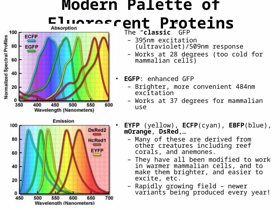
• The “classic” GFP– 395nm excitation (ultraviolet)/509nm
response– Works at 28 degrees (too cold for
mammalian cells)
• EGFP: enhanced GFP– Brighter, more convenient 484nm excitation– Works at 37 degrees for mammalian use
• EYFP (yellow), ECFP(cyan), EBFP(blue), mOrange, DsRed,…– Many of these are derived from other
creatures including reef corals, and anemones.
– They have all been modified to work in warmer mammalian cells, and to make them brighter, and easier to excite, etc.
– Rapidly growing field – newer variants being produced every year!
Modern Palette of Fluorescent Proteins

Imaging Intra-Cellular Transport
• Vesicles are miniature “taxicabs” carrying cargo within the cells
• They slide over cytoskeletal fibers as they go from one place to another
• They have molecular equivalents of “address labels” so there is considerable specificity
http://www.ohsu.edu/croet/faculty/banker/bankerlab.html
Vesicle transportin a neuron

Considerations for Live-Cell Imaging• The microscopy should not hurt/kill the cells:
– Toxicity of the fluorescent label• Could change the chemical function of molecule of interest• Could be outright toxic to the cell(s)
– Photo-toxicity (damage caused by light)• Ultraviolet disrupts molecules• Infrared heats up tissue• Prolonged exposure to any wavelength can be bad
– Configuration of microscope• Inverted microscopes preferable
– In vitro imaging: • Need instrumentation for keeping cells alive in a dish• Temperature, humidity, oxygen, Carbon dioxide,
– In vivo imaging:• Much harder – image a part of a living animal• Surgical techniques to provide optical access the tissue of interest
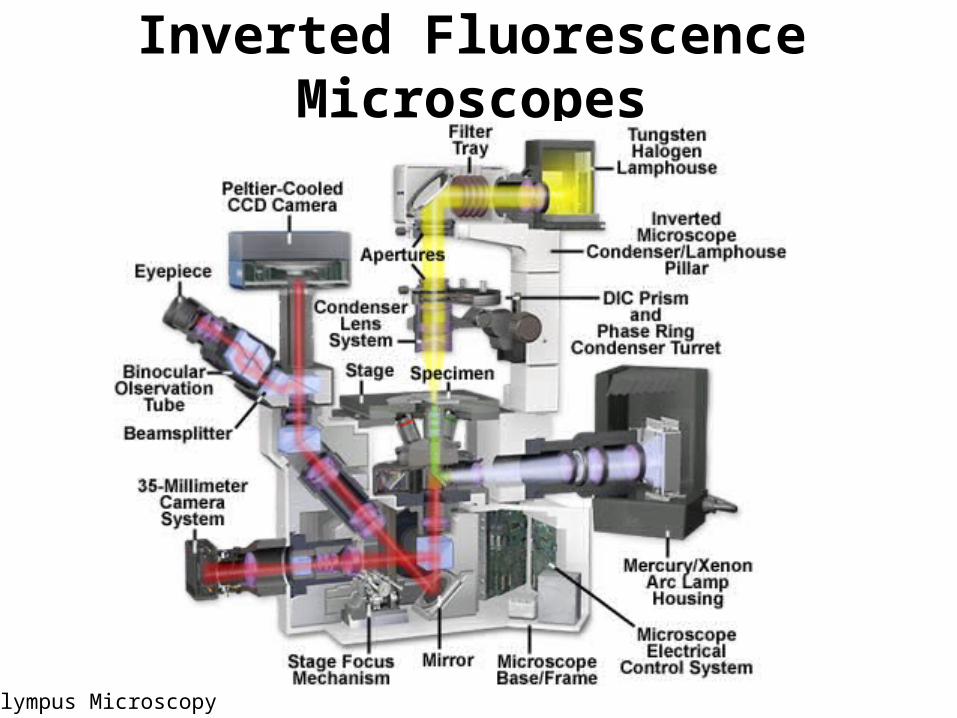
Inverted Fluorescence Microscopes
Olympus Microscopy

Recap: Fluorescence• Molecular imaging systems
– Produce spatial maps capturing distributions/locations of specific molecules
• Interactions of molecules with light– Intrinsic imaging– Imaging with contrast agents,
especially fluorophores– Fluorescence is a hugely important
phenomenon• Imaging genes and gene activity
– FISH: fluorescence in-situ hybridization
• Imaging proteins – the products of gene activity– Immunofluorescence: The use of
fluorescently conjugated antibodies to “tag” specific proteins of interest
– Multiplexing: Simultaneous use of multiple tags to image multiple proteins preserving relative context
1E2E3E4E
0E
Abs
orpt
ion
Non-radiativeTransition / Loss
RadiativeTransition

Multi-Photon Fluorescence• Basic Idea:
– Hit the molecule with multiple photons, say 2, simultaneously
– The molecule cannot distinguish this excitation from a single photon with twice the energy
2E hv
(2 )E h v
2 2E hv
0E
Non-radiativetransition
Emission
3-photon works the same way
Short-livedVirtualState
1E hv

What does it take to achieve multi-photon fluorescence?
• The probability of two photons hitting a molecule at nearly the same time, (within 10-18 seconds), is extremely low!
• Need to achieve a super high concentration of photons– Megawatt per cubic micrometer
• Can’t do this on a sustained basis!– Idea #1: Use a pulsed laser, so average
energy is still low enough to make specimen damage negligible
• 100mW– Idea #2: Concentrate the energy in space by
using a lens• Intense focal spot
– Idea #3: Concentrate the energy in time by using ultra-short pulses from a “mode locked laser”
• 50-100 femtosecond pulses• 1 femtosecond = 10-15 sec • Expensive stuff ( $100,000)!
Lens
Laser PulseFocal Spot
Laser
T
W
P

What does it Buy Us?• A dye that would ordinarily
require ultraviolet excitation at 400nm, could now be excited using two infrared 800nm photons– Infrared is dramatically less
damaging to molecular structures compared to ultraviolet
• No chemical disruption, just causes a little heating
– Infrared is absorbed and scattered much less, so one can achieve deeper penetration into tissue
– Ability to image autofluorescence without damage
– It allows “super localization”• We’ll explain that shortly

Localized Multi-photon Response
Probability of simultaneous absorption falls off steeply away from the focal volume, localizing the response along the optical axis 3-D Imaging Possible!
1P
2P

Reduced Photobleaching
• Single-photon excitation happens throughput the cone of illumination
• Multi-photon excitation only happens near the focus
negligible photobleaching above/below the plane of focus
Lens

Example: In-vivo Imaging of Brain Tumors
Courtesy: Dr. R. Jain, MGH
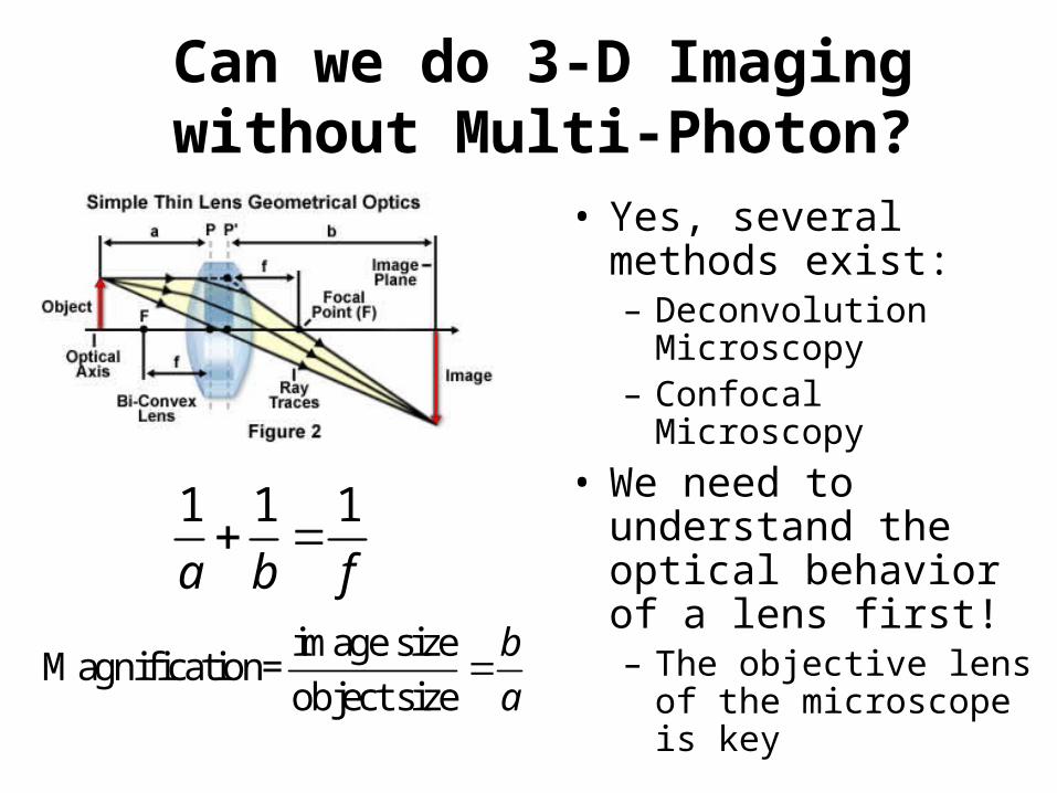
Can we do 3-D Imaging without Multi-Photon?
• Yes, several methods exist:– Deconvolution Microscopy– Confocal Microscopy
• We need to understand the optical behavior of a lens first!– The objective lens of the
microscope is key
1 1 1
a b f
image sizeMagnification=
object size
b
a

Light sheet microscopySanti, P. A.Light sheet fluorescence microscopy: A review. Journal of Histochemistry and Cytochemistry 59: 129-138 (2011). Dr. Santi introduces a nicely composed review article that covers the basic principles of light sheet microscopy that includes a historical perspective, instrumentation requirements, and details about how to process specimens for imaging.

LSM vs. TPM
Bouchard, M. B., et al. (2015). "Swept confocally-aligned planar excitation (SCAPE) microscopy for high-speed volumetric imaging of behaving organisms." Nat Photon advance online publication.
We report a three-dimensional microscopy technique—swept, confocally-aligned planar excitation (SCAPE) microscopy—that allows volumetric imaging of living samples at ultrahigh speeds. Although confocal and two-photon microscopy have revolutionized biomedical research, current implementations are costly, complex and limited in their ability to image three-dimensional volumes at high speeds. Light-sheet microscopy techniques using two-objective, orthogonal illumination and detection require a highly constrained sample geometry and either physical sample translation or complex synchronization of illumination and detection planes. In contrast, SCAPE microscopy acquires images using an angled, swept light sheet in a single-objective, en face geometry. Unique confocal descanning and image rotation optics map this moving plane onto a stationary high-speed camera, permitting completely translationless three-dimensional imaging of intact samples at rates exceeding 20 volumes per second. We demonstrate SCAPE microscopy by imaging spontaneous neuronal firing in the intact brain of awake behaving mice, as well as freely moving transgenic Drosophila larvae.

Numerical Aperture (N.A.)
sin.. nAN
n = refractive index of medium
Medium Refractive Index
Air 1.0
Water 1.33
Immersion oil 1.55

Airy patterns and resolution
Also known as the point-spread function

Obtaining 3-D Structure without the Multi-Photon Effect
• “Confocal Microscopy”– Name comes from
“conjugate foci” of lenses: f1 and f2
• Basic idea:– Put a tiny pinhole at the
conjugate focus f2
– Almost all of the light from the point in the specimen “squeezes through” the pinhole1f
2f
Point in the specimen
Pinhole

Effect of Pinhole
Better axial resolution, butFewer photons

Optical Slices
• Move the z stage up/down• At each z value, scan across the x-y field to collect an “optical slice”• A “stack” of optical slices is a volumetric (3-D) image

How do we view a 3-D image?• The computer screen is
two-dimensional, so we have to project the 3-D volume I(x,y,z) onto a 2-D image P(x,y)– Two basic choices to make:
• Projection angle– Simplest: Aligned with axes– Best: Oblique angles
• Projection formula/algorithm– Sum / Average / Median– Max / Min– Surface Rendering
( , )P x y
( , , )I x y z

Viewing by Projections
m5.0
Neuron: TR054Z1
Step Size:
Zoom: 1.0
Dimension:
512x480x323
The “maximum value” projection is most commonly used for fluorescence data
max{ }
( , ) max ( , , )z
I x y I x y z

Volumetric Rendering• Choose a viewing angle• Ray casting: Shoot rays back
into the volume from each pixel in P(x,y)– Compute an intensity value by
summation / max / min / …etc.• Good: Objective, since we’re not
“messing with” the data• Bad: Computationally expensive
– We often desire to rotate the object interactively to look from different angles
• Could be slow on a regular computer
– Expensive hardware accelerators and parallel computation algorithms available for real-time volume rendering.
( , )P x y
( , , )I x y z
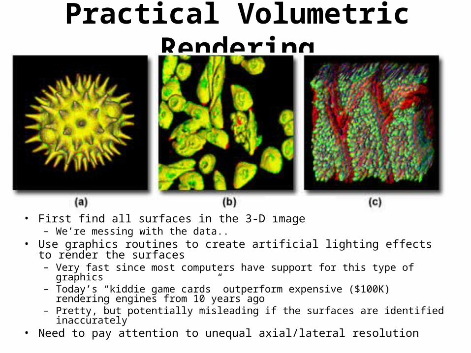
Practical Volumetric Rendering
• First find all surfaces in the 3-D image– We’re messing with the data..
• Use graphics routines to create artificial lighting effects to render the surfaces– Very fast since most computers have support for this type of graphics– Today’s “kiddie game cards” outperform expensive ($100K) rendering engines
from 10 years ago– Pretty, but potentially misleading if the surfaces are identified inaccurately
• Need to pay attention to unequal axial/lateral resolution

Faster Confocals• Spinning Disk Systems
– Nipkow Disks• Scans lots of points at
once using a rotating disk with a spiral array of holes, and a CCD camera instead of photomultipler tubes
– The basis for all modern high-throughput microscopes
http://zeiss-campus.magnet.fsu.edu/tutorials/spinningdisk/spinningdiskfundamentals/index.html

Impure Channels• There are basically two kinds of impurities to
consider:– Case 1: Morphologically impure
• The fluorescent label is not specific enough• We can get two or more types of “things” in a channel• Solution 1 (preferred): work with the biologist to either choose
different things to label, or different labels if at all possible• Solution 2: develop algorithms that can handle morphologically
mixed data
– Case 2: Spectrally impure • The fluorescent labels are specific, but their spectra overlap
heavily• Solution 1 (preferred): seek out alternative fluorescent labels• Solution 2: computationally “unmix” the data

Dealing with Overlapping Spectra
Nucleus: histone GFP FusionActin filaments: fluorescein conjugated phalloidinThe peaks are separated by only 7nm !
2
1

Dealing with Overlapping Spectra
“Unmixing Result”: A1 and A2
1 1 2 2( , , ) ( , , ) ( ) ( , , ) ( )S x y z A x y z R A x y z R
Compute A1 and A2 at each pixel subject to constraint A1 + A2 = 1
Reference Spectra

Ultimate Optical Microscope of the Future
• Isotropic and high-resolution sampling of 3-D space (x, y, z)
– Recent microscopes have broken past the Rayleigh resolution limit
• No wasted photons – 100% detection
• Complete spectrum at each pixel– Measure absorption & emission spectrum– Complete flexibility to shape the excitation spectrum– Complete flexibility to capture and analyze the emission
spectrum
• Complete lifetime response at each pixel– Photon counting hardware at each detector– Time response at different spectral wavelengths
• Multiple modalities looking at the same specimen– One of the holy grails that continues to be pursued
0.61. .
RN A