ECE5655 FM4 Lab 2

March 8, 2016

Contents

Linear Algebra with Python 2A Quick Look at Sympy for Linear Algebra . . . . . . . . . . . . . . . . . . . . . . . . . . . . 3

Problem 1 5

Problem 2 5

Problem 3 7Part a . . . . . . . . . . . . . . . . . . . . . . . . . . . . . . . . . . . . . . . . . . . . . . . . . 8Part b . . . . . . . . . . . . . . . . . . . . . . . . . . . . . . . . . . . . . . . . . . . . . . . . . 8Part c . . . . . . . . . . . . . . . . . . . . . . . . . . . . . . . . . . . . . . . . . . . . . . . . . 8

Problem 4: Real-Time Gold Code with LUT and Pulse Shaping 8PN Code Generation . . . . . . . . . . . . . . . . . . . . . . . . . . . . . . . . . . . . . . . . . 8Pulse Shaping and Upsampling by Four . . . . . . . . . . . . . . . . . . . . . . . . . . . . . . 9

Import the Full CA Gold Code Matrix . . . . . . . . . . . . . . . . . . . . . . . . . . . 9Python Model of the Required C Code Used for Pulse Shaping . . . . . . . . . . . . . 9

Support Code and Examples . . . . . . . . . . . . . . . . . . . . . . . . . . . . . . . . . . . . 10Function that Writes Gold Code Headers . . . . . . . . . . . . . . . . . . . . . . . . . 10Write FIR Header Files . . . . . . . . . . . . . . . . . . . . . . . . . . . . . . . . . . . 12Write Raised Cosine and Root Raised Cosine Headers for 4 Samples/Bit . . . . . . . . 13

Process Data In a CSV File Exported from Analog Discovery 14Get on with the Problem 4 Lab Write Up . . . . . . . . . . . . . . . . . . . . . . . . . . . . . 16

In [1]: %pylab inline

#%matplotlib qt # for popout plots

from __future__ import division # use so 1/2 = 0.5, etc.

import ssd

import scipy.signal as signal

from IPython.display import Image, SVG

Populating the interactive namespace from numpy and matplotlib

In [103]: pylab.rcParams[’savefig.dpi’] = 100 # default 72

#pylab.rcParams[’figure.figsize’] = (6.0, 4.0) # default (6,4)

#%config InlineBackend.figure_formats=[’png’] # default for inline viewing

#%config InlineBackend.figure_formats=[’svg’] # SVG inline viewing

%config InlineBackend.figure_formats=[’pdf’] # render pdf figs for LaTeX

1

Linear Algebra with Python

To get started with numerical linear algebra calculations in Python we need to import the linear algebramodule from, scipy.linalg.

In [9]: import scipy.linalg as linalg

We can now create matrices as 2D numpy ndarrays:

In [12]: A = array([[1,2,3,4],[5,6,7,8]])

A

Out[12]: array([2, 3])

In [13]: AT = A.T

AT

Out[13]: array([[1, 5],

[2, 6],

[3, 7],

[4, 8]])

In [15]: B = array([[1,2],[4,9]])

BI = linalg.inv(B)

In [16]: B

Out[16]: array([[1, 2],

[4, 9]])

In [17]: BI

Out[17]: array([[ 9., -2.],

[-4., 1.]])

In [18]: dot(B,BI)

Out[18]: array([[ 1., 0.],

[ 0., 1.]])

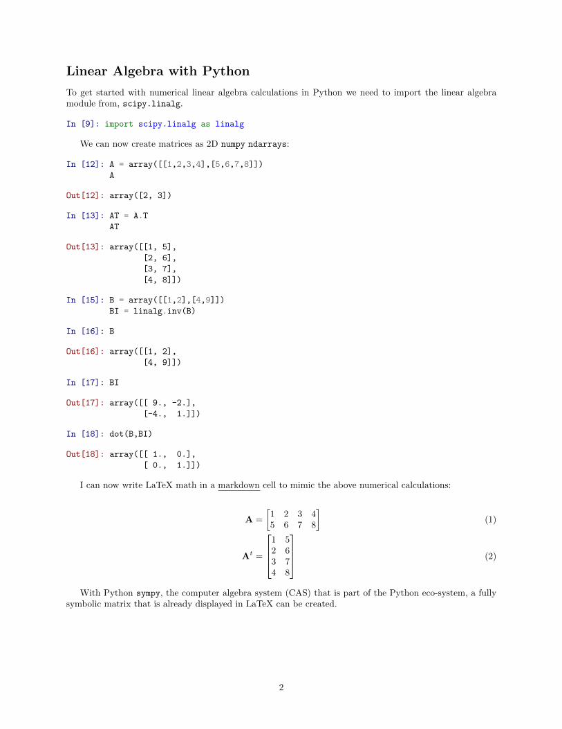
I can now write LaTeX math in a markdown cell to mimic the above numerical calculations:

A =

[1 2 3 45 6 7 8

](1)

At =

1 52 63 74 8

(2)

With Python sympy, the computer algebra system (CAS) that is part of the Python eco-system, a fullysymbolic matrix that is already displayed in LaTeX can be created.

2

A Quick Look at Sympy for Linear Algebra

In [5]: from IPython.display import display

from sympy.interactive import printing

printing.init_printing(use_latex=’mathjax’)

import sympy as sym

A, B, C = sym.symbols("A B C")

In [8]: A = sym.Matrix([[1,2,3,4],[5,6,7,8]])

A

Out[8]: [1 2 3 45 6 7 8

]In [9]: A.T

Out[9]: 1 52 63 74 8

In [11]: a,b,c,d = sym.symbols("a b c d")

In [13]: # All symbolic matrix

B = sym.Matrix([[a,b],[c,d]])

B

Out[13]: [a bc d

]In [17]: B.det()

Out[17]:

ad− bc

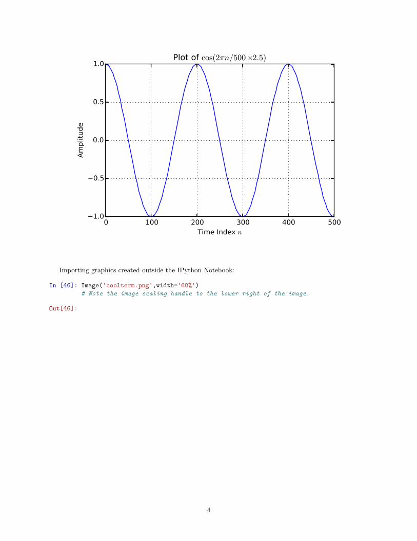
A sample plot:

In [44]: n = arange(0,500)

x = cos(2*pi*n/500*2.5)

plot(n,x)

xlabel(r’Time Index $n$’)

ylabel(r’Amplitude’)

title(r’Plot of $\cos(2\pi n/500 \times 2.5)$’)

grid();

3

0 100 200 300 400 500Time Index n

1.0

0.5

0.0

0.5

1.0

Am

plit

ude

Plot of cos(2πn/500×2.5)

Importing graphics created outside the IPython Notebook:

In [46]: Image(’coolterm.png’,width=’60%’)

# Note the image scaling handle to the lower right of the image.

Out[46]:

4

Problem 1

Develop a C calling C function that implements the numerical calculation

C = A−B

using the data type int16 t, where

A =[a2 + (a + 1)2 + (a + 2)2 + · · ·+ (2a− 1)2

]B =

[b2 + (b + 1)2 + (b + 2)2 + · · ·+ (2b− 1)2

]You can perform calculations right in the notebook using Python with the magic %pylab filling the

workspace with numpy for array-based mathematics and matplotlib for 2D and 3D interactive graphics.

Problem 2

Wolfram Mathematica or WolframAlpha on the Web can be useful too. The images imported in the notebookwere captured on my iPad using the WolframAlpha for iPad app:

5

In [49]: Image(’inv3by3.png’,width=’40%’)

Out[49]:

In [48]: Image(’det3by3.png’,width=’40%’)

Out[48]:

6

Some C Code

int main(void){int16_t x = 0;

char my_debug[80];

float32_t buffer[4] = {1.0,2.3,3.5,-6.7};static float32_t AData[2*4] = {1.0f,2.0f,3.0f,4.0f,5.0f,6.0f,7.0f,8.0f};static float32_t ATData[4*2] = {0.0f,0.0f,0.0f,0.0f,0.0f,0.0f,0.0f,0.0f};arm_matrix_instance_f32 A = {2,4,AData};arm_matrix_instance_f32 AT = {4,2,ATData};

Problem 3

In this program you will convert the pseudo-code for a square-root algorithm shown below into C code forfloat32 t input/output variables.

Approximate square root with bisection method

INPUT: Argument x, endpoint values a, b, such that a < b

OUTPUT: value which differs from sqrt(x) by less than 1

done = 0

a = 0

b = square root of largest possible argument (e.g. ~216).

7

c = -1

do {c_old = c

c = (a+b)/2

if (c*c == x) {done = 1

} else if (c*c < x) {a = c

} else {b = c

}} while (!done) && (c != c_old)

return c

Part a

Code the above square root algorithm in C. Profile you code using the test values 23, 56.5, and 1023.7. Runtests at compiler optimization Level 0 and Level 3. Note: You will need to establish a stopping condition,as the present form is designed for integer math. I suggest modifying the line:

if (c*c == x) { to something like if (fabs(c*c - x) <= max_error) }

where max-error is intially set to . Realize that this value directly impacts the execution speed, asa smaller error requirement means more iterations are required. See if you can find the accuracy of thestandard library square root.

Part b

Compare the performance of your square root function at O3 with the standard math library function forfloat (float32 t), using float sqrtf(float x).

• Tests were run using . . .

Part c

Compare the performance of your square root function at O3 to the M4 FPU intrinsic function float32 t

sqrtf(float x).

• Tests were run using . . .

Problem 4: Real-Time Gold Code with LUT and Pulse Shaping

Pseudo-random sequences find application in digital communications system. The most common sequencesare known as M-sequences, where M stands for maximal length. A Gold Code formed by exclusive ORing twoM sequences of the same length but of different phases. For example Gold codes of length 1023 are uniquelyassigned to the GPS satellites so that the transmissions from the satellites may share the same frequencyspectrum, but be separated by the properties of the Gold codes which make nearly mutually orthogonal. Inthis problem you start by building an M-sequence generator in C.

PN Code Generation

Implement as described and test via GPIO pins. You may also want to send output to the terminal andimport into Python to plot and verify properties. I will want to see waveforms on the scope and/or logicanalyzer. Use the synch pulse output a synch signal for the scope

8

Pulse Shaping and Upsampling by Four

A prototype of the upsampling can be implemented using Python, right here in the notebook. We will usethe actual CA code sequence. This requires importing the entire matrix then just using one row as the bitstream.

In [16]: import digitalcom as dc

In [35]: len(filt_states)

Out[35]: 48

Import the Full CA Gold Code Matrix

In [4]: camat = loadtxt(’ca1thru37.txt’,dtype=int16,unpack=True)

In [4]: # Check the size of the matrix

camat.shape

Out[4]: (37L, 1023L)

In [5]: # Check the data type

camat.dtype

Out[5]: dtype(’int16’)

Python Model of the Required C Code Used for Pulse Shaping

This code resides in the codec ISR.

In [61]: # Pulse shaping filter at 4x oversampling

b_src = dc.sqrt_rc_imp(4,0.35) # 0.35 <==> excess bandwidth factor

# Use a gold code, say CA 4

d = 10000*(2*camat[4-1,:]- 1) # level shift to create 1000 * a +/-1 sequence

# Create array to hold filtered output signal values

x = zeros(4*len(d))

# Create array to hold FIR filter states, one less than the number of taps

# CMSIS-DSP manages this for you

filt_states = zeros(len(b_src)-1)

CA_idx = 0

CA_code_period = 1023

for k in range(4*len(d)):

if mod(k,4) == 0:

# Filter one signal sample

x_filt, filt_states = signal.lfilter(b_src,1,[d[CA_idx]],zi=filt_states)

x[k] = x_filt

else:

x_filt, filt_states = signal.lfilter(b_src,1,[0],zi=filt_states)

x[k] = x_filt

# Increment index on CA code modulo 1023

CA_idx = mod(CA_idx+1,CA_code_period)

In [72]: figure(figsize=(6,5))

subplot(211)

plot(x[1000:1500])

xlabel(r’Samples’)

ylabel(r’Amplitude Values’)

9

title(r’Filter Output Samples Upsampled and Scaled for D/A’)

grid();

subplot(212)

psd(x,2**10,48) # Actual fs = 48 kHz

ylabel(r’PSD (dB/Hz)’)

xlabel(r’Frequency (kHz)’)

tight_layout()

0 100 200 300 400 500

Samples

20000

15000

10000

5000

0

5000

10000

15000

20000

Am

plit

ude V

alu

es

Filter Output Samples Upsampled and Scaled for D/A

0 5 10 15 20 25

Frequency (kHz)

100

1020304050607080

PSD

(dB

/Hz)

Support Code and Examples

Function that Writes Gold Code Headers

In [6]: def CA_code_header(fname_out,Nca):

"""

Write 1023 bit CA (Gold) Code Header Files

Mark Wickert February 2015

"""

ca = loadtxt(’ca1thru37.txt’,dtype=int16,usecols=(Nca-1,),unpack=True)

M = 1023 # code period

N = 23 # code bits per line

10

Sca = ’ca’ + str(Nca)

f = open(fname_out,’wt’)

f.write(’//define a CA code\n\n’)

f.write(’#include <stdint.h>\n\n’)

f.write(’#ifndef N_CA\n’)

f.write(’#define N_CA %d\n’ % M)

f.write(’#endif\n’)

f.write(’/*******************************************************************/\n’);

f.write(’/* 1023 Bit CA Gold Code %2d */\n’\

% Nca);

f.write(’int8_t ca%d[N_CA] = {’ % Nca)

kk = 0;

for k in range(M):

#k_mod = k % M

if (kk < N-1) and (k < M-1):

f.write(’%d,’ % ca[k])

kk += 1

elif (kk == N-1) & (k < M-1):

f.write(’%d,\n’ % ca[k])

if k < M:

if Nca < 10:

f.write(’ ’)

else:

f.write(’ ’)

kk = 0

else:

f.write(’%d’ % ca[k])

f.write(’};\n’)

f.write(’/*******************************************************************/\n’)

f.close()

In [ ]: CA_code_header(’CA_1.h’,1) #write a header for CA code 1

CA_code_header(’CA_12.h’,12) #write a header for CA code 12

In [6]: import digitalcom as dc

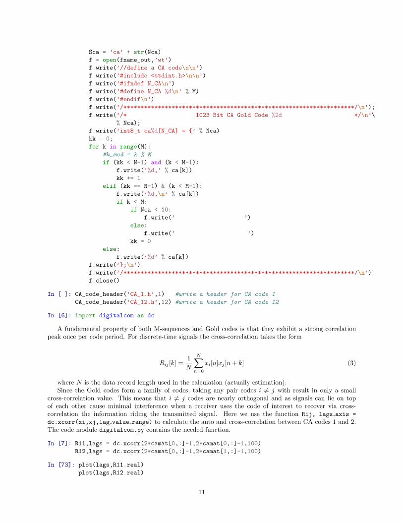
A fundamental property of both M-sequences and Gold codes is that they exhibit a strong correlationpeak once per code period. For discrete-time signals the cross-correlation takes the form

Rij [k] =1

N

N∑n=0

xi[n]xj [n + k] (3)

where N is the data record length used in the calculation (actually estimation).Since the Gold codes form a family of codes, taking any pair codes i 6= j with result in only a small

cross-correlation value. This means that i 6= j codes are nearly orthogonal and as signals can lie on topof each other cause minimal interference when a receiver uses the code of interest to recover via cross-correlation the information riding the transmitted signal. Here we use the function Rij, lags axis =

dc.xcorr(xi,xj,lag value range) to calculate the auto and cross-correlation between CA codes 1 and 2.The code module digitalcom.py contains the needed function.

In [7]: R11,lags = dc.xcorr(2*camat[0,:]-1,2*camat[0,:]-1,100)

R12,lags = dc.xcorr(2*camat[0,:]-1,2*camat[1,:]-1,100)

In [73]: plot(lags,R11.real)

plot(lags,R12.real)

11

xlabel(r’Lag $k$ in auto/coss-correlation’)

ylabel(r’Normalized Correlation Amplitude’)

title(r’CA Code Correlation Properties Over One Period’)

legend((r’Autocorr of CA1’,r’Crosscorr of CA1/2’),loc=’best’,)

grid();

100 50 0 50 100

Lag k in auto/coss-correlation

0.2

0.0

0.2

0.4

0.6

0.8

1.0

1.2

Norm

aliz

ed C

orr

ela

tion A

mplit

ude

CA Code Correlation Properties Over One Period

Autocorr of CA1

Crosscorr of CA1/2

Write FIR Header Files

In [11]: def FIR_header(fname_out,h):

"""

Write FIR Filter Header Files

Mark Wickert February 2015

"""

M = len(h)

N = 3 # Coefficients per line

f = open(fname_out,’wt’)

f.write(’//define a FIR coeffient Array\n\n’)

f.write(’#include <stdint.h>\n\n’)

f.write(’#ifndef M_FIR\n’)

f.write(’#define M_FIR %d\n’ % M)

f.write(’#endif\n’)

f.write(’/************************************************************************/\n’);

f.write(’/* FIR Filter Coefficients */\n’);

f.write(’float32_t h_FIR[M_FIR] = {’)

kk = 0;

for k in range(M):

12

#k_mod = k % M

if (kk < N-1) and (k < M-1):

f.write(’%15.12f,’ % h[k])

kk += 1

elif (kk == N-1) & (k < M-1):

f.write(’%15.12f,\n’ % h[k])

if k < M:

f.write(’ ’)

kk = 0

else:

f.write(’%15.12f’ % h[k])

f.write(’};\n’)

f.write(’/************************************************************************/\n’)

f.close()

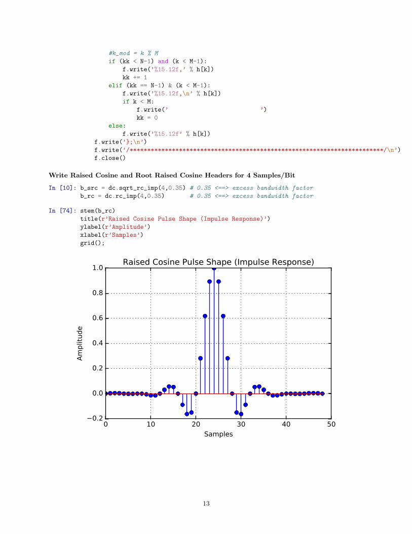
Write Raised Cosine and Root Raised Cosine Headers for 4 Samples/Bit

In [10]: b_src = dc.sqrt_rc_imp(4,0.35) # 0.35 <==> excess bandwidth factor

b_rc = dc.rc_imp(4,0.35) # 0.35 <==> excess bandwidth factor

In [74]: stem(b_rc)

title(r’Raised Cosine Pulse Shape (Impulse Response)’)

ylabel(r’Amplitude’)

xlabel(r’Samples’)

grid();

0 10 20 30 40 50

Samples

0.2

0.0

0.2

0.4

0.6

0.8

1.0

Am

plit

ude

Raised Cosine Pulse Shape (Impulse Response)

13

Process Data In a CSV File Exported from Analog Discovery

In [94]: t_rc,xL_rc,xR_rc = loadtxt(’AD_test.csv’,delimiter=’,’,unpack=True,skiprows=6)

The first 6 rows contain file data, i.e.,

#Digilent WaveForms Oscilloscope Acquisition

#Device Name: Discovery2

#Serial Number: SN:210321A1882E

#Date Time: 2016-03-08 11:16::25.070

Time (s),Channel 1 (V),Channel 2 (V)

-0.01463125,-0.15396102452950045,-0.11439924582729083

-0.014625000000000001,-0.15462511758046754,-0.11202808120137372

-0.01461875,-0.15362897800401654,-0.11033439218286108

In this case 8000 samples were captured at a sampling rate of 80 kHz.

Time Domain

In [104]: plot(t_rc[3200:4800]*1000,xL_rc[3200:4800])

title(r’Waveform Captured From Codec Output’)

ylabel(r’Amplitude’)

xlabel(r’Time (ms)’)

grid();

10 5 0 5 10

Time (ms)

0.3

0.2

0.1

0.0

0.1

0.2

0.3

Am

plit

ude

Waveform Captured From Codec Output

14

Eye Plot

In [105]: # Eyeplot obtain by resampling capture at 80 kHz back to 48 kHz

# which results in 4 samples per bit (clock errors involved here)

dc.eye_plot(dc.farrow_resample(xL_rc[1000:2000],80,48),2*4)

Out[105]: 0

0 1 2 3 4 5 6 7 8

Time Index - n

0.3

0.2

0.1

0.0

0.1

0.2

0.3

Am

plit

ude

Eye Plot

Power Spectral Density Estimate Using Short 8192 Data Record

In [106]: psd(xL_rc,2**10,80);

xlabel(r’Frequency (kHz)’)

Out[106]: <matplotlib.text.Text at 0xbe68b38>

15

0 5 10 15 20 25 30 35 40

Frequency (kHz)

100

90

80

70

60

50

40

30

20

Pow

er

Spect

ral D

ensi

ty (

dB

/Hz)

Get on with the Problem 4 Lab Write Up

In [ ]:

16