ece 421 introduction to signal processing · – frequency sampling of discrete time signals...
TRANSCRIPT
ECE 421Introduction to Signal Processing
Dror BaronAssistant Professor
Dept. of Electrical and Computer Engr.North Carolina State University, NC, USA
Discrete Fourier Transform

Roadmap
3
We have seen– Chapter 1 – from analog to digital and back– Chapter 2 – discrete time signals & systems; correlation– Chapter 3 – z-transforms; transfer functions; one-sided z– Chapter 4 – Fourier transforms– Chapter 5 – frequency domain analysis of LTI systems– Chapter 6 – sampling, reconstruction, end-to-end systems, …
About to discuss Chapter 7– Frequency sampling of discrete time signals discrete Fourier
transform (DFT)– Implementing linear filters with DFT– Application to frequency analysis

Frequency Sampling of Discrete Time Signals
[Reading material: Section 7.1]

Challenges for discrete time signals
5
Fourier representations of aperiodic and periodic discrete time signals are helpful
BUT…
Aperiodic?– Impractical to know X(ω) for infinitely many ω∈[-π, π]
Periodic?– Most signals “in the wild” aren’t periodic
Need tools for finite duration signals
What tools for finite duration signals?
6
Finite duration signals motivate discrete Fourier transform (DFT)
Another motivation/perspective is frequency sampling
Frequency Sampling
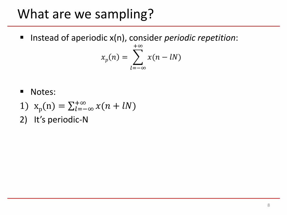
What are we sampling?
8
Instead of aperiodic x(n), consider periodic repetition:
𝑥𝑥𝑝𝑝 𝑛𝑛 = �𝑙𝑙=−∞
+∞
𝑥𝑥(𝑛𝑛 − 𝑙𝑙𝑙𝑙)
Notes:1) xp(n) = ∑𝑙𝑙=−∞+∞ 𝑥𝑥(𝑛𝑛 + 𝑙𝑙𝑙𝑙)2) It’s periodic-N

Fourier series for xp(n)
9
Periodic repetition xp(n) periodic can take its Fourier series
𝑥𝑥𝑝𝑝 𝑛𝑛 = ∑𝑘𝑘=0𝑁𝑁−1 𝐶𝐶𝑘𝑘𝑒𝑒𝑗𝑗𝑗𝜋𝜋𝑘𝑘𝜋𝜋/𝑁𝑁
𝐶𝐶𝑘𝑘 = 1𝑁𝑁∑𝑘𝑘=0𝑁𝑁−1 𝑥𝑥𝑝𝑝(𝑛𝑛) 𝑒𝑒−𝑗𝑗𝑗𝜋𝜋𝑘𝑘𝜋𝜋/𝑁𝑁
Will soon see relation between X(2πk/N) and Ck

Sampling X(ω)
10
Recall 𝑋𝑋 𝜔𝜔 = ∑𝜋𝜋=−∞+∞ 𝑥𝑥(𝑛𝑛)𝑒𝑒−𝑗𝑗𝜔𝜔𝜋𝜋
Let’s take N samples of X(ω) It’s periodic focus on range ω∈[0,2π) ω=2πk/N
𝑋𝑋 𝑗𝜋𝜋𝑘𝑘𝑁𝑁
= ∑𝜋𝜋=−∞+∞ 𝑥𝑥(𝑛𝑛)𝑒𝑒−𝑗𝑗(2𝜋𝜋𝜋𝜋𝑁𝑁 )𝜋𝜋
= ⋯+ ∑𝜋𝜋=−𝑁𝑁−1 𝑥𝑥(𝑛𝑛)𝑒𝑒−𝑗𝑗(2𝜋𝜋𝜋𝜋𝑁𝑁 )𝜋𝜋+∑𝜋𝜋=0𝑁𝑁−1 𝑥𝑥(𝑛𝑛)𝑒𝑒−𝑗𝑗(2𝜋𝜋𝜋𝜋𝑁𝑁 )𝜋𝜋 + ⋯
= ∑𝑙𝑙=−∞+∞ ∑𝜋𝜋=𝑙𝑙𝑁𝑁𝑙𝑙𝑁𝑁+𝑁𝑁−1 𝑥𝑥(𝑛𝑛)𝑒𝑒−𝑗𝑗2𝜋𝜋𝜋𝜋𝜋𝜋𝑁𝑁
= ∑𝑖𝑖=0𝑁𝑁−1∑𝑙𝑙=−∞+∞ 𝑥𝑥(𝑙𝑙𝑙𝑙 + 𝑖𝑖)𝑒𝑒−𝑗𝑗2𝜋𝜋𝜋𝜋𝑁𝑁 (𝑙𝑙𝑁𝑁+𝑖𝑖) n=lN+i
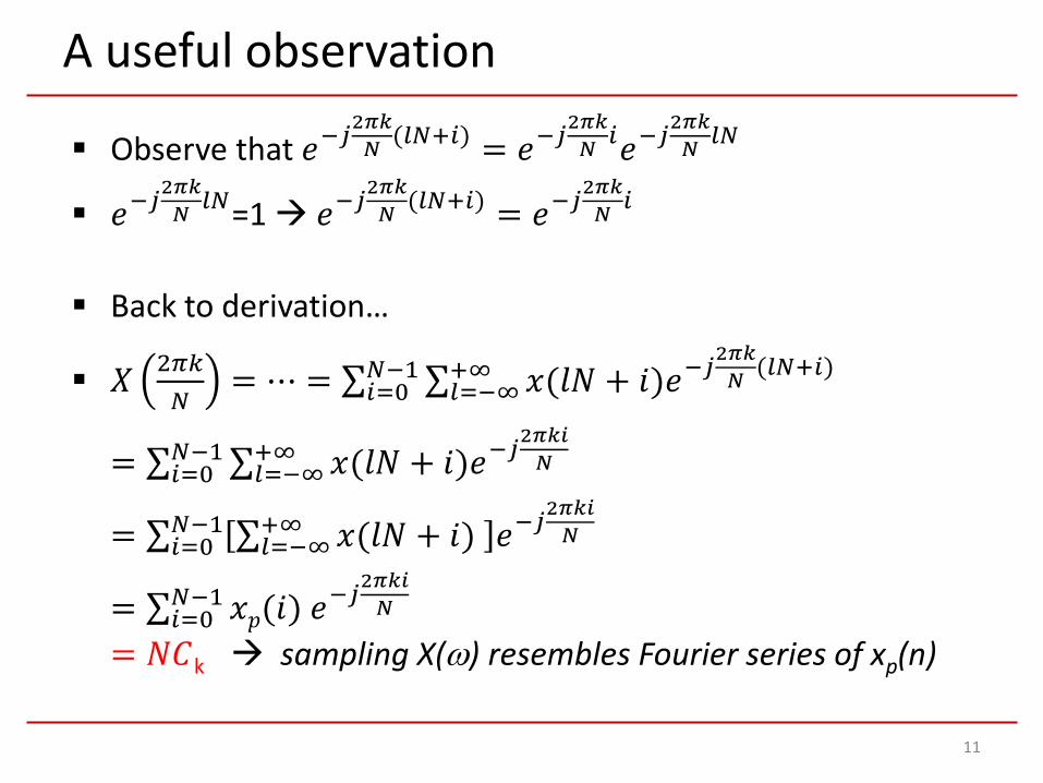
A useful observation
11
Observe that 𝑒𝑒−𝑗𝑗2𝜋𝜋𝜋𝜋𝑁𝑁 (𝑙𝑙𝑁𝑁+𝑖𝑖) = 𝑒𝑒−𝑗𝑗
2𝜋𝜋𝜋𝜋𝑁𝑁 𝑖𝑖𝑒𝑒−𝑗𝑗
2𝜋𝜋𝜋𝜋𝑁𝑁 𝑙𝑙𝑁𝑁
𝑒𝑒−𝑗𝑗2𝜋𝜋𝜋𝜋𝑁𝑁 𝑙𝑙𝑁𝑁=1 𝑒𝑒−𝑗𝑗
2𝜋𝜋𝜋𝜋𝑁𝑁 (𝑙𝑙𝑁𝑁+𝑖𝑖) = 𝑒𝑒−𝑗𝑗
2𝜋𝜋𝜋𝜋𝑁𝑁 𝑖𝑖
Back to derivation…
𝑋𝑋 𝑗𝜋𝜋𝑘𝑘𝑁𝑁
= ⋯ = ∑𝑖𝑖=0𝑁𝑁−1∑𝑙𝑙=−∞+∞ 𝑥𝑥(𝑙𝑙𝑙𝑙 + 𝑖𝑖)𝑒𝑒−𝑗𝑗2𝜋𝜋𝜋𝜋𝑁𝑁 (𝑙𝑙𝑁𝑁+𝑖𝑖)
= ∑𝑖𝑖=0𝑁𝑁−1∑𝑙𝑙=−∞+∞ 𝑥𝑥(𝑙𝑙𝑙𝑙 + 𝑖𝑖)𝑒𝑒−𝑗𝑗2𝜋𝜋𝜋𝜋𝜋𝜋𝑁𝑁
= ∑𝑖𝑖=0𝑁𝑁−1 ∑𝑙𝑙=−∞+∞ 𝑥𝑥(𝑙𝑙𝑙𝑙 + 𝑖𝑖) 𝑒𝑒−𝑗𝑗2𝜋𝜋𝜋𝜋𝜋𝜋𝑁𝑁
= ∑𝑖𝑖=0𝑁𝑁−1 𝑥𝑥𝑝𝑝(𝑖𝑖) 𝑒𝑒−𝑗𝑗2𝜋𝜋𝜋𝜋𝜋𝜋𝑁𝑁
= 𝑙𝑙𝐶𝐶k sampling X(ω) resembles Fourier series of xp(n)
Discussion
12
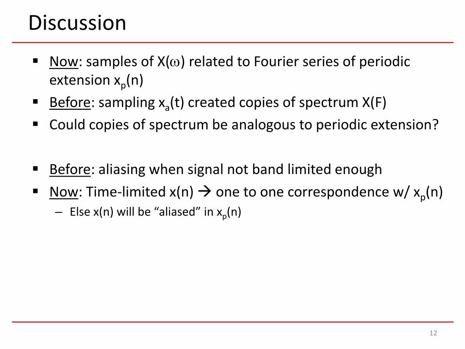
Now: samples of X(ω) related to Fourier series of periodic extension xp(n)
Before: sampling xa(t) created copies of spectrum X(F) Could copies of spectrum be analogous to periodic extension?
Before: aliasing when signal not band limited enough Now: Time-limited x(n) one to one correspondence w/ xp(n)
– Else x(n) will be “aliased” in xp(n)

Example 7.1.1
13
Consider x(n)=anu(n), |a|<1
Fourier transform, 𝑋𝑋 𝜔𝜔 = 11−𝑎𝑎𝑒𝑒−𝑗𝑗𝜔𝜔
Take N samples, 𝑋𝑋 2𝜋𝜋𝑘𝑘/𝑙𝑙 = 11−𝑎𝑎𝑒𝑒−𝑗𝑗2𝜋𝜋𝜋𝜋/𝑁𝑁
Can compute xp(n) from Ck=1𝑁𝑁𝑋𝑋 2𝜋𝜋𝑘𝑘/𝑙𝑙
Is x(n) identical to xp(n)?– Will show 𝑥𝑥𝑝𝑝 𝑛𝑛 = ⋯ = ∑𝑙𝑙=−∞0 𝑎𝑎𝜋𝜋−𝑙𝑙𝑁𝑁 = ⋯ = 𝑎𝑎𝜋𝜋
1−𝑎𝑎𝑁𝑁
Large N aN<<1 small “aliasing”

Frequency Interpolation?
Motivation
15
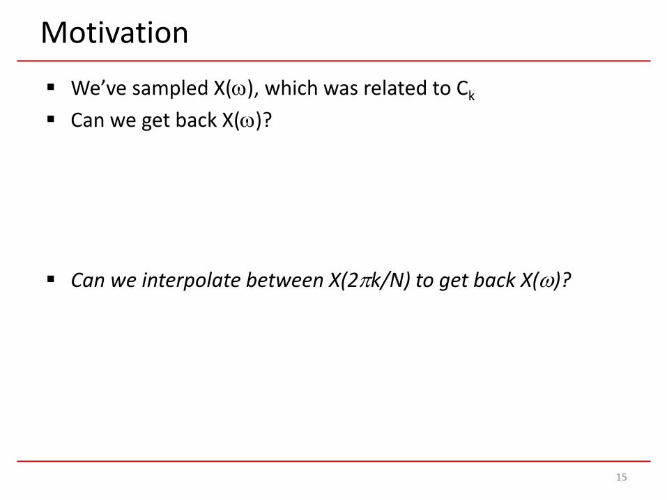
We’ve sampled X(ω), which was related to Ck
Can we get back X(ω)?
Can we interpolate between X(2πk/N) to get back X(ω)?
Interpolation
16
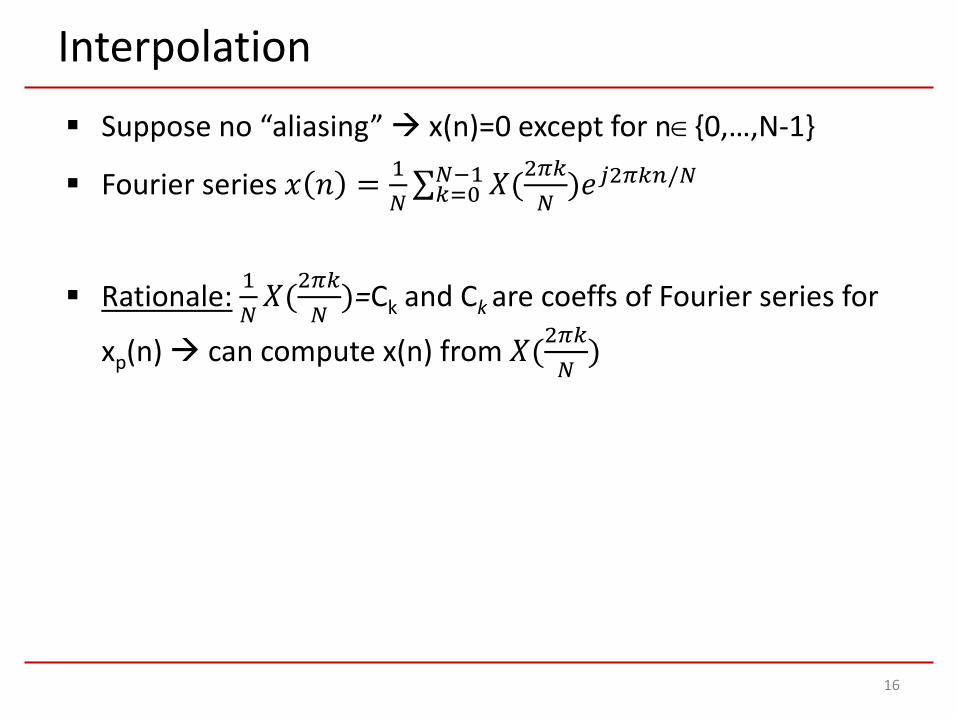
Suppose no “aliasing” x(n)=0 except for n∈{0,…,N-1}
Fourier series 𝑥𝑥 𝑛𝑛 = 1𝑁𝑁∑𝑘𝑘=0𝑁𝑁−1𝑋𝑋(𝑗𝜋𝜋𝑘𝑘
𝑁𝑁)𝑒𝑒𝑗𝑗𝑗𝜋𝜋𝑘𝑘𝜋𝜋/𝑁𝑁
Rationale: 1𝑁𝑁𝑋𝑋(𝑗𝜋𝜋𝑘𝑘
𝑁𝑁)=Ck and Ck are coeffs of Fourier series for
xp(n) can compute x(n) from 𝑋𝑋(𝑗𝜋𝜋𝑘𝑘𝑁𝑁
)

Interpolation
17
Suppose no “aliasing” x(n)=0 except for n∈{0,…,N-1}
Fourier series 𝑥𝑥 𝑛𝑛 = 1𝑁𝑁∑𝑘𝑘=0𝑁𝑁−1𝑋𝑋(𝑗𝜋𝜋𝑘𝑘
𝑁𝑁)𝑒𝑒𝑗𝑗𝑗𝜋𝜋𝑘𝑘𝜋𝜋/𝑁𝑁
Let’s substitute Fourier series into computation of X(ω) 𝑋𝑋 𝜔𝜔 = ∑𝜋𝜋=−∞+∞ 𝑥𝑥(𝑛𝑛)𝑒𝑒−𝑗𝑗𝜔𝜔𝜋𝜋
= ∑𝜋𝜋=0𝑁𝑁−1 𝑥𝑥(𝑛𝑛)𝑒𝑒−𝑗𝑗𝜔𝜔𝜋𝜋
= ∑𝜋𝜋=0𝑁𝑁−1 1𝑁𝑁∑𝑘𝑘=0𝑁𝑁−1𝑋𝑋(𝑗𝜋𝜋𝑘𝑘
𝑁𝑁)𝑒𝑒𝑗𝑗𝑗𝜋𝜋𝑘𝑘𝜋𝜋/𝑁𝑁 𝑒𝑒−𝑗𝑗𝜔𝜔𝜋𝜋
= ∑𝑘𝑘=0𝑁𝑁−1𝑋𝑋(𝑗𝜋𝜋𝑘𝑘𝑁𝑁
) 1𝑁𝑁∑𝜋𝜋=0𝑁𝑁−1 𝑒𝑒
𝑗𝑗2𝜋𝜋𝜋𝜋𝜋𝜋𝑁𝑁 −𝑗𝑗𝜔𝜔𝜋𝜋
= ∑𝑘𝑘=0𝑁𝑁−1𝑋𝑋(𝑗𝜋𝜋𝑘𝑘𝑁𝑁
) 1𝑁𝑁∑𝜋𝜋=0𝑁𝑁−1 𝑒𝑒−𝑗𝑗 𝜔𝜔−𝑗𝜋𝜋𝑘𝑘/𝑁𝑁 𝜋𝜋
P(ω −2𝜋𝜋𝑘𝑘/𝑙𝑙)

Let’s compute P(ω)
18
𝑃𝑃 𝜔𝜔 = 1𝑁𝑁∑𝜋𝜋=0𝑁𝑁−1 𝑒𝑒−𝑗𝑗𝜔𝜔𝜋𝜋
= 1𝑁𝑁1−𝑒𝑒−𝑗𝑗𝜔𝜔𝑁𝑁
1−𝑒𝑒−𝑗𝑗𝜔𝜔
= 1𝑁𝑁𝑒𝑒−𝑗𝑗𝜔𝜔𝑁𝑁/2 𝑒𝑒+𝑗𝑗𝜔𝜔𝑁𝑁/2−𝑒𝑒−𝑗𝑗𝜔𝜔𝑁𝑁/2
𝑒𝑒−𝑗𝑗𝜔𝜔/2 𝑒𝑒+𝑗𝑗𝜔𝜔/2−𝑒𝑒−𝑗𝑗𝜔𝜔/2
= 1𝑁𝑁sin 𝜔𝜔𝑁𝑁/𝑗sin 𝜔𝜔 /𝑗
𝑒𝑒−𝑗𝑗𝜔𝜔(𝑁𝑁−1)/𝑗
Substituting into X(ω) expression:
𝑋𝑋 𝜔𝜔 = �𝑘𝑘=0
𝑁𝑁−1
𝑋𝑋2𝜋𝜋𝑘𝑘𝑙𝑙
𝑃𝑃(𝜔𝜔 − 2𝜋𝜋𝑘𝑘/𝑙𝑙)
Resembles convolution with LPF but it’s Dirichlet kernel (resembles sinc + artifacts due to periodic X(ω))
The Discrete Fourier Transform

Finite duration perspective
20
Recall two perspectives– Finite duration signals motivate discrete Fourier transform (DFT) – Frequency sampling also motivates DFT
We’ve sampled the Fourier transform, let’s consider x(n) with finite duration L≤N
𝑥𝑥𝑝𝑝 𝑛𝑛 = �𝑥𝑥 𝑛𝑛 , 0 ≤ 𝑛𝑛 ≤ 𝐿𝐿 − 10, 𝐿𝐿 ≤ 𝑛𝑛 ≤ 𝑙𝑙 − 1
For L<N must perform zero padding (add N-L zeros)– Allows to analyze length-L signal with as many freqs as we want– For example, N>>L helps make smooth-looking plot
The DFT
21
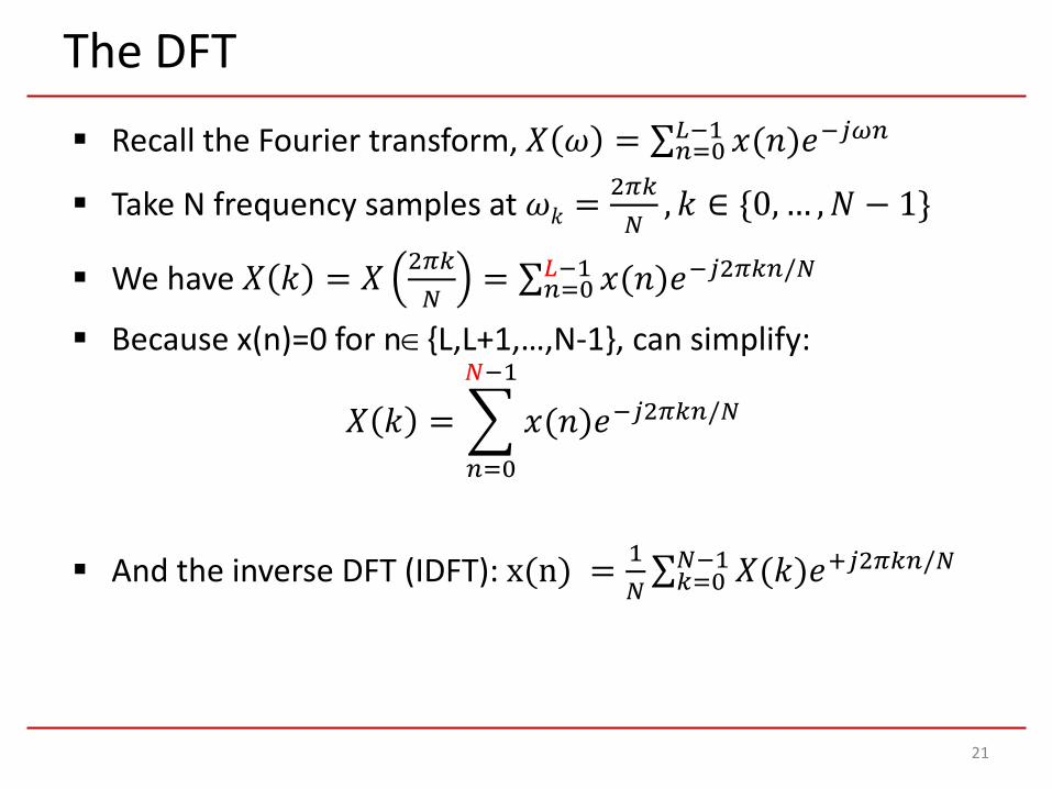
Recall the Fourier transform, 𝑋𝑋 𝜔𝜔 = ∑𝜋𝜋=0𝐿𝐿−1 𝑥𝑥(𝑛𝑛)𝑒𝑒−𝑗𝑗𝜔𝜔𝜋𝜋
Take N frequency samples at 𝜔𝜔𝑘𝑘 = 𝑗𝜋𝜋𝑘𝑘𝑁𝑁
,𝑘𝑘 ∈ {0, … ,𝑙𝑙 − 1}
We have 𝑋𝑋 𝑘𝑘 = 𝑋𝑋 𝑗𝜋𝜋𝑘𝑘𝑁𝑁
= ∑𝜋𝜋=0𝐿𝐿−1 𝑥𝑥(𝑛𝑛)𝑒𝑒−𝑗𝑗𝑗𝜋𝜋𝑘𝑘𝜋𝜋/𝑁𝑁
Because x(n)=0 for n∈{L,L+1,…,N-1}, can simplify:
𝑋𝑋 𝑘𝑘 = �𝜋𝜋=0
𝑁𝑁−1
𝑥𝑥(𝑛𝑛)𝑒𝑒−𝑗𝑗𝑗𝜋𝜋𝑘𝑘𝜋𝜋/𝑁𝑁
And the inverse DFT (IDFT): x(n) = 1𝑁𝑁∑𝑘𝑘=0𝑁𝑁−1𝑋𝑋(𝑘𝑘)𝑒𝑒+𝑗𝑗𝑗𝜋𝜋𝑘𝑘𝜋𝜋/𝑁𝑁

Active learning (example 7.1.2)
22
Consider finite duration signal, x 𝑛𝑛 = � 1, 0 ≤ 𝑛𝑛 ≤ 𝐿𝐿 − 10, 𝐿𝐿 ≤ 𝑛𝑛 ≤ 𝑙𝑙 − 1
Fill in gaps while computing Fourier transform 𝑋𝑋 𝜔𝜔 = ∑𝜋𝜋=−∞+∞ 𝑥𝑥(𝑛𝑛)𝑒𝑒−𝑗𝑗𝜔𝜔𝜋𝜋
= ∑𝜋𝜋=?????? 𝑥𝑥(𝑛𝑛)𝑒𝑒−𝑗𝑗𝜔𝜔𝜋𝜋 what are the ranges?
= ∑𝜋𝜋=?????? 1𝑒𝑒−𝑗𝑗𝜔𝜔𝜋𝜋
= 1−???1−???
geometric series
Can be expressed 𝑋𝑋 𝜔𝜔 = sin 𝜔𝜔𝐿𝐿/𝑗sin 𝜔𝜔/𝑗
𝑒𝑒−𝑗𝑗𝜔𝜔(𝐿𝐿−1)/𝑗
DFT as a Transform[Reading material: Sections 7.1.3, 7.1.4, & 7.2.2]

Linear algebra 101
24
Column vector 𝑣𝑣 =𝑎𝑎1⋮𝑎𝑎𝑙𝑙
Matrix 𝐴𝐴 = 𝑎𝑎 𝑏𝑏𝑐𝑐 𝑑𝑑 , more generally M rows, N columns
– One row/column implies row/column vector
Matrix vector product (examples):
– 1 22 3
12 = 1 � 1 + 2 � 2
2 � 1 + 3 � 2 = 58
– 1 2 3456
= 1 � 4 + 2 � 5+ 3 � 6 = 32

Matrix inverse
25
For matrix A such that y=Ax, inverse A-1 satisfies A-1y=x Can show AA-1=A-1A=I
– I identity matrix (ones on diagonal, else zero)
Matrix (usually) invertible if it’s square
Example:
– 𝐴𝐴 = 1 00 2
– 𝐴𝐴−1 = 1 00 1/2
– 𝐴𝐴𝐴𝐴−1 = 1 00 2
1 00 1/2 = 1 � 1 + 0 � 0 1 � 0 + 0 � 1/2
0 � 1 + 2 � 0 0 � 0 + 2 � 1/2 = 1 00 1
identity matrix

Back to DFT
26
Recall – DFT: 𝑋𝑋 𝑘𝑘 = ∑𝜋𝜋=0𝑁𝑁−1 𝑥𝑥(𝑛𝑛)𝑒𝑒−𝑗𝑗𝑗𝜋𝜋𝑘𝑘𝜋𝜋/𝑁𝑁
– IDFT: x(n) = 1𝑁𝑁∑𝑘𝑘=0𝑁𝑁−1𝑋𝑋(𝑘𝑘)𝑒𝑒+𝑗𝑗𝑗𝜋𝜋𝑘𝑘𝜋𝜋/𝑁𝑁
Define auxiliary variable, wN=e-j2π/N
– DFT: 𝑋𝑋 𝑘𝑘 = ∑𝜋𝜋=0𝑁𝑁−1 𝑥𝑥(𝑛𝑛)𝑤𝑤𝑁𝑁+𝑘𝑘𝜋𝜋
– IDFT: x(n) = 1𝑁𝑁∑𝑘𝑘=0𝑁𝑁−1𝑋𝑋(𝑘𝑘)𝑤𝑤𝑁𝑁−𝑘𝑘𝜋𝜋
DFT matrix form:
𝑋𝑋𝑙𝑙 =𝑋𝑋(0)⋮
𝑋𝑋(𝑙𝑙 − 1)=
𝑤𝑤𝑁𝑁0�0 ⋯ 𝑤𝑤𝑁𝑁0�(𝑁𝑁−1)
⋮ ⋱ ⋮𝑤𝑤𝑁𝑁
(𝑁𝑁−1)�0 ⋯ 𝑤𝑤𝑁𝑁(𝑁𝑁−1)�(𝑁𝑁−1)
𝑥𝑥(0)⋮
𝑥𝑥(𝑙𝑙 − 1)= 𝑊𝑊𝑙𝑙𝑥𝑥𝑙𝑙
WN
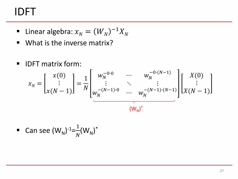
IDFT
27
Linear algebra: 𝑥𝑥𝑙𝑙 = 𝑊𝑊𝑙𝑙−1𝑋𝑋𝑙𝑙
What is the inverse matrix?
IDFT matrix form:
𝑥𝑥𝑙𝑙 =𝑥𝑥(0)⋮
𝑥𝑥(𝑙𝑙 − 1)=
1𝑙𝑙
𝑤𝑤𝑁𝑁−0�0 ⋯ 𝑤𝑤𝑁𝑁−0�(𝑁𝑁−1)
⋮ ⋱ ⋮𝑤𝑤𝑁𝑁−(𝑁𝑁−1)�0 ⋯ 𝑤𝑤𝑁𝑁
−(𝑁𝑁−1)�(𝑁𝑁−1)
𝑋𝑋(0)⋮
𝑋𝑋(𝑙𝑙 − 1)
Can see (WN)-1=1𝑁𝑁
(WN)*
(WN)*

Active learning (example 7.1.3)
28
Signal x=[0 1 2 3]T
– T for transpose (make vertical by flipping)
1) What is w4? (Recall wN=e-j2π/N)
2) Fill in powers of w4
𝑊𝑊4 =𝑤𝑤4 𝑤𝑤4𝑤𝑤4 𝑤𝑤4
𝑤𝑤4 𝑤𝑤4𝑤𝑤4 𝑤𝑤4𝑤𝑤4 𝑤𝑤4
𝑤𝑤4 𝑤𝑤4
𝑤𝑤4 𝑤𝑤4𝑤𝑤4 𝑤𝑤4
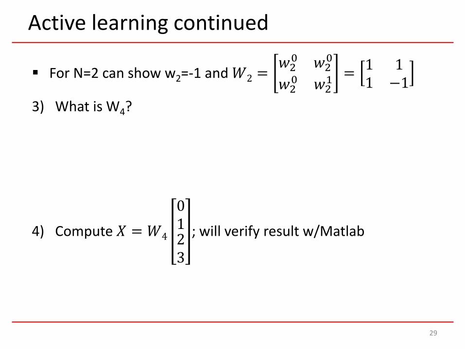
Active learning continued
29
For N=2 can show w2=-1 and 𝑊𝑊2 =𝑤𝑤𝑗0 𝑤𝑤𝑗0
𝑤𝑤𝑗0 𝑤𝑤𝑗1= 1 1
1 −13) What is W4?
4) Compute 𝑋𝑋 = 𝑊𝑊4
0123
; will verify result w/Matlab

DFT and Other Transforms
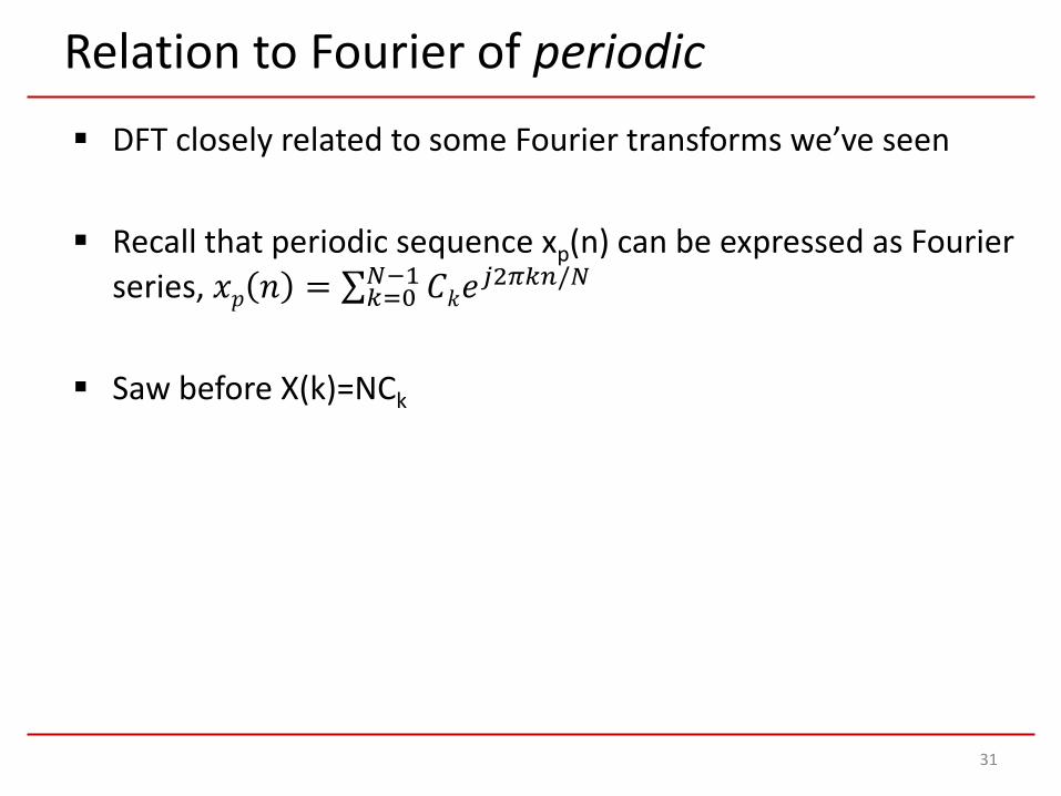
Relation to Fourier of periodic
31
DFT closely related to some Fourier transforms we’ve seen
Recall that periodic sequence xp(n) can be expressed as Fourier series, 𝑥𝑥𝑝𝑝 𝑛𝑛 = ∑𝑘𝑘=0𝑁𝑁−1 𝐶𝐶𝑘𝑘𝑒𝑒𝑗𝑗𝑗𝜋𝜋𝑘𝑘𝜋𝜋/𝑁𝑁
Saw before X(k)=NCk
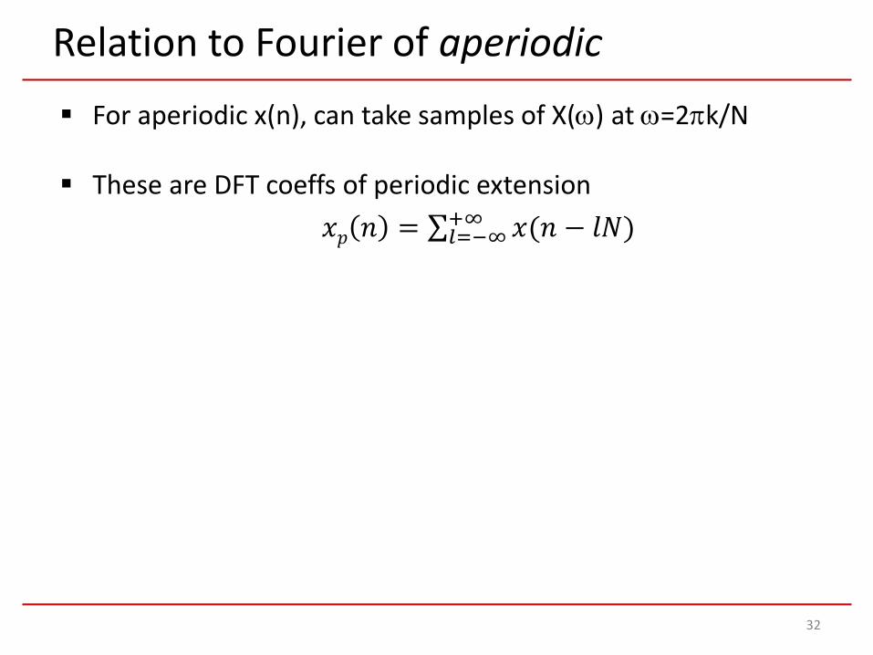
Relation to Fourier of aperiodic
32
For aperiodic x(n), can take samples of X(ω) at ω=2πk/N
These are DFT coeffs of periodic extension 𝑥𝑥𝑝𝑝 𝑛𝑛 = ∑𝑙𝑙=−∞+∞ 𝑥𝑥(𝑛𝑛 − 𝑙𝑙𝑙𝑙)

More relations
33
Can relate DFT to z transform using z=ej2πk/N
– Details in book
Relation to periodic continuous time signal– Suppose signal is band limited– N samples capture all information about xa(t)– N series coeffs capture all information– These coeffs related to DFT coeffs

Circular Convolution
DFT properties
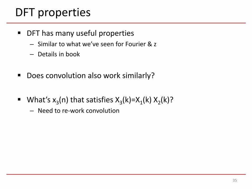
35
DFT has many useful properties– Similar to what we’ve seen for Fourier & z– Details in book
Does convolution also work similarly?
What’s x3(n) that satisfies X3(k)=X1(k) X2(k)?– Need to re-work convolution
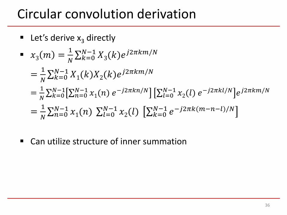
Circular convolution derivation
36
Let’s derive x3 directly
𝑥𝑥3 𝑚𝑚 = 1𝑁𝑁∑𝑘𝑘=0𝑁𝑁−1𝑋𝑋3(𝑘𝑘)𝑒𝑒𝑗𝑗𝑗𝜋𝜋𝑘𝑘𝜋𝜋/𝑁𝑁
= 1𝑁𝑁∑𝑘𝑘=0𝑁𝑁−1𝑋𝑋1(𝑘𝑘)𝑋𝑋2(𝑘𝑘)𝑒𝑒𝑗𝑗𝑗𝜋𝜋𝑘𝑘𝜋𝜋/𝑁𝑁
= 1𝑁𝑁∑𝑘𝑘=0𝑁𝑁−1 ∑𝜋𝜋=0𝑁𝑁−1 𝑥𝑥1(𝑛𝑛) 𝑒𝑒−𝑗𝑗𝑗𝜋𝜋𝑘𝑘𝜋𝜋/𝑁𝑁 ∑𝑙𝑙=0𝑁𝑁−1 𝑥𝑥2(𝑙𝑙) 𝑒𝑒−𝑗𝑗𝑗𝜋𝜋𝑘𝑘𝑙𝑙/𝑁𝑁 𝑒𝑒𝑗𝑗𝑗𝜋𝜋𝑘𝑘𝜋𝜋/𝑁𝑁
= 1𝑁𝑁∑𝜋𝜋=0𝑁𝑁−1 𝑥𝑥1(𝑛𝑛) ∑𝑙𝑙=0𝑁𝑁−1 𝑥𝑥2(𝑙𝑙) ∑𝑘𝑘=0𝑁𝑁−1 𝑒𝑒−𝑗𝑗𝑗𝜋𝜋𝑘𝑘(𝜋𝜋−𝜋𝜋−𝑙𝑙)/𝑁𝑁
Can utilize structure of inner summation
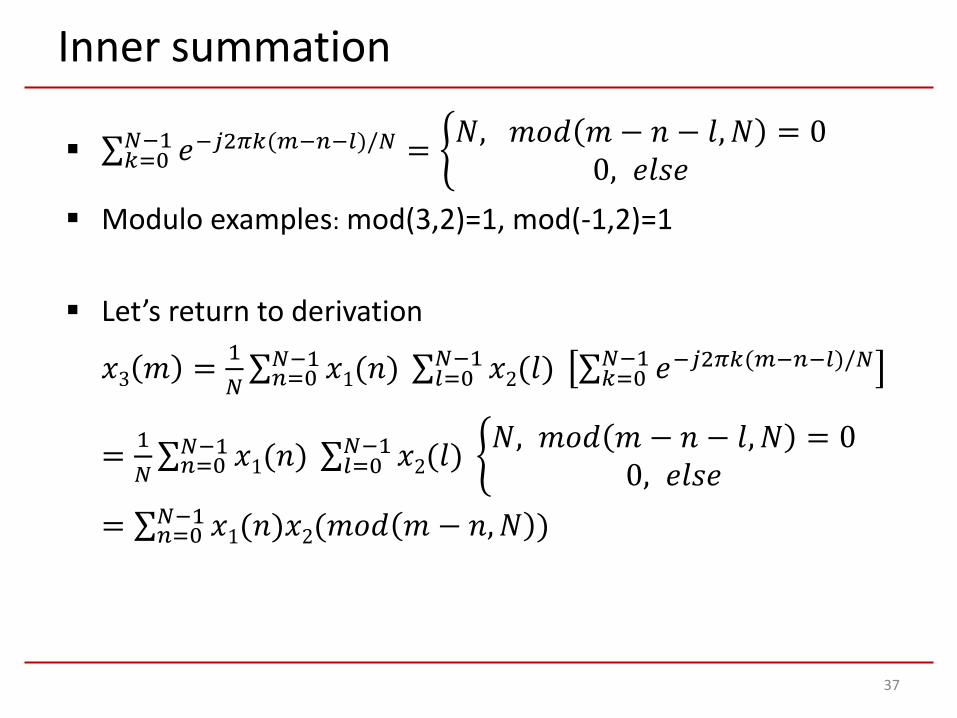
Inner summation
37
∑𝑘𝑘=0𝑁𝑁−1 𝑒𝑒−𝑗𝑗𝑗𝜋𝜋𝑘𝑘(𝜋𝜋−𝜋𝜋−𝑙𝑙)/𝑁𝑁 = �𝑙𝑙, 𝑚𝑚𝑚𝑚𝑑𝑑 𝑚𝑚 − 𝑛𝑛 − 𝑙𝑙,𝑙𝑙 = 00, 𝑒𝑒𝑙𝑙𝑒𝑒𝑒𝑒
Modulo examples: mod(3,2)=1, mod(-1,2)=1
Let’s return to derivation
𝑥𝑥3 𝑚𝑚 = 1𝑁𝑁∑𝜋𝜋=0𝑁𝑁−1 𝑥𝑥1(𝑛𝑛) ∑𝑙𝑙=0𝑁𝑁−1 𝑥𝑥2(𝑙𝑙) ∑𝑘𝑘=0𝑁𝑁−1 𝑒𝑒−𝑗𝑗𝑗𝜋𝜋𝑘𝑘(𝜋𝜋−𝜋𝜋−𝑙𝑙)/𝑁𝑁
= 1𝑁𝑁∑𝜋𝜋=0𝑁𝑁−1 𝑥𝑥1(𝑛𝑛) ∑𝑙𝑙=0𝑁𝑁−1 𝑥𝑥2(𝑙𝑙) �𝑙𝑙, 𝑚𝑚𝑚𝑚𝑑𝑑 𝑚𝑚 − 𝑛𝑛 − 𝑙𝑙,𝑙𝑙 = 0
0, 𝑒𝑒𝑙𝑙𝑒𝑒𝑒𝑒 = ∑𝜋𝜋=0𝑁𝑁−1 𝑥𝑥1(𝑛𝑛)𝑥𝑥2(𝑚𝑚𝑚𝑚𝑑𝑑 𝑚𝑚 − 𝑛𝑛,𝑙𝑙 )
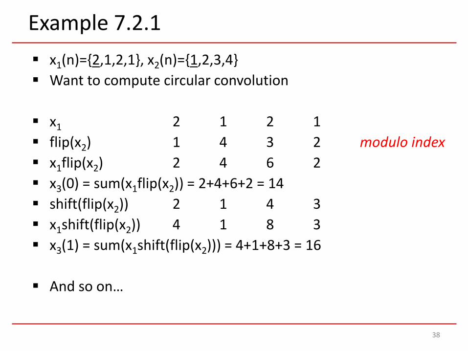
Example 7.2.1
38
x1(n)={2,1,2,1}, x2(n)={1,2,3,4} Want to compute circular convolution
x1 2 1 2 1 flip(x2) 1 4 3 2 modulo index x1flip(x2) 2 4 6 2 x3(0) = sum(x1flip(x2)) = 2+4+6+2 = 14 shift(flip(x2)) 2 1 4 3 x1shift(flip(x2)) 4 1 8 3 x3(1) = sum(x1shift(flip(x2))) = 4+1+8+3 = 16
And so on…

Example 7.2.1 continued
39
Can be performed in Matlab:– x1=[2 1 2 1];– x2=[1 2 3 4];– x1f=fft(x1);– x2f=fft(x2);– x3f=x1f.*x2f;– x3=ifft(x3f);

More Properties of DFT[Reading material: Section 7.2]

Time reversal property
41
Time reversal: x((-n))N=x(N-n) ↔ X((-k))N=X(N-k)– Subscript denotes modulo-N
Example: Matlab– x(n)={0,1,2,3} x=[0 1 2 3];– x((-n))N={0,3,2,1} xr=[0 3 2 1];– X(k)={6,-2+2j,-2,-2-2j} fft(x)– DFT of flipped version? fft(xr)

Circular time shift property
42
Circular time shift: x((n-l))N ↔ X(k)e-j2πkl/N
x1={0,1,2,3} x2={3,0,1,2} DFT{x2}={6,2+2j,2,2-2j}
Can verify in Matlab: fft(x1).*exp(-j*2*pi/N*[0:3])
More
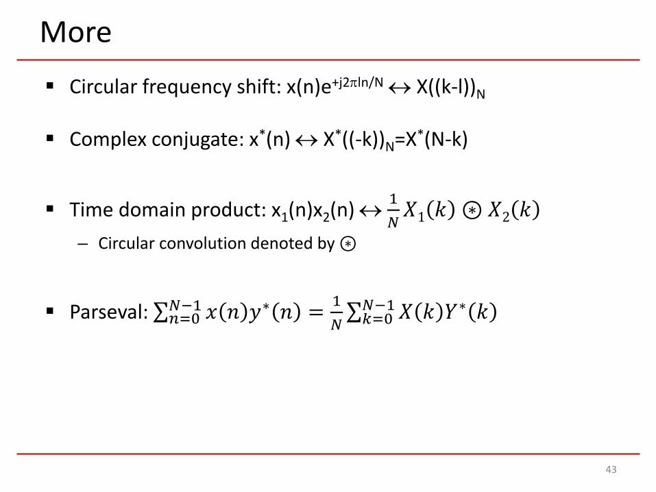
43
Circular frequency shift: x(n)e+j2πln/N ↔ X((k-l))N
Complex conjugate: x*(n) ↔ X*((-k))N=X*(N-k)
Time domain product: x1(n)x2(n) ↔ 1𝑁𝑁𝑋𝑋1 𝑘𝑘 ⊛ 𝑋𝑋2 𝑘𝑘
– Circular convolution denoted by ⊛
Parseval: ∑𝜋𝜋=0𝑁𝑁−1 𝑥𝑥 𝑛𝑛 𝑦𝑦∗ 𝑛𝑛 = 1𝑁𝑁∑𝑘𝑘=0𝑁𝑁−1𝑋𝑋 𝑘𝑘 𝑌𝑌∗ 𝑘𝑘
Linear Filters Using DFT[Reading material: Section 7.3]

Linear vs. circular convolution
45
We’ve seen how to compute circular convolution using DFT– Fast Fourier transform (FFT) – fast algorithm for computing DFT– Circular convolution using FFT is quite efficient
Linear convolution appears in many applications
𝑦𝑦 𝑛𝑛 = �𝑘𝑘=−∞
+∞
ℎ 𝑛𝑛 − 𝑘𝑘 𝑥𝑥(𝑘𝑘)
Applications include digital filters in communication / control systems (e.g., audio equalization)
Will compute linear convolution using circular convolution

Why is this useful?
46
The convolution equation for linear filtering seems simple– It’s probably simple to implement and fast– Why care?
Consider multipath– Suppose we sample at 100M samples/sec– Path lengths differ by 1 kM– Speed of light 300,000 kM/s– Time difference 1/300,000 sec 3.33 usec 333 samples– May need filter w/1,000 taps thousands of computations per sample
Using FFT (N*log(N)) operations) N=1,000 log(N) << N much more efficient
Example
47
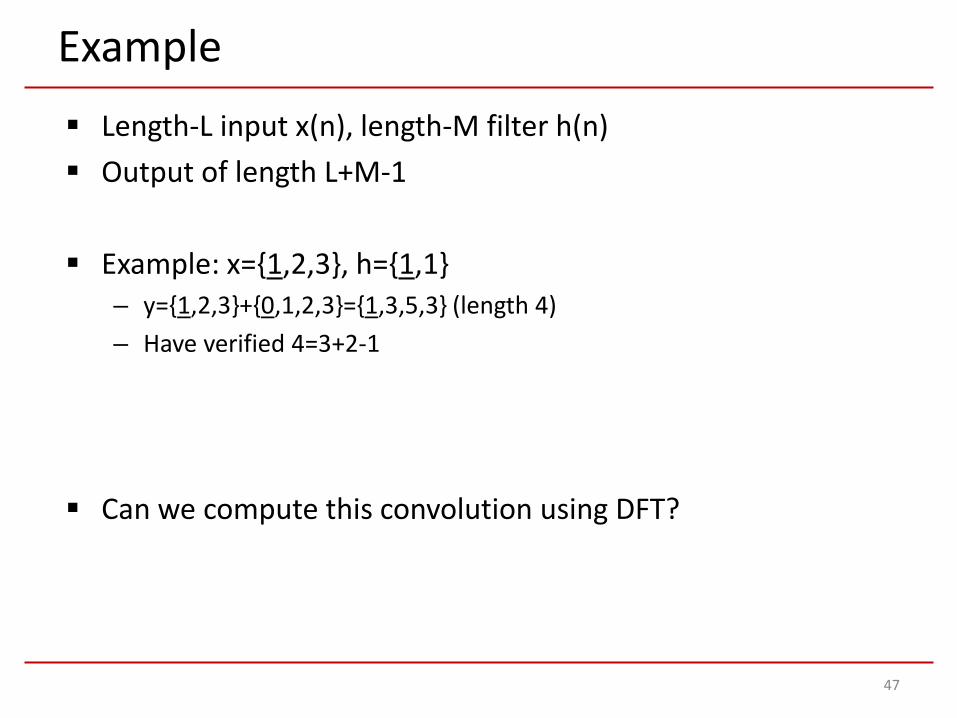
Length-L input x(n), length-M filter h(n) Output of length L+M-1
Example: x={1,2,3}, h={1,1}– y={1,2,3}+{0,1,2,3}={1,3,5,3} (length 4)– Have verified 4=3+2-1
Can we compute this convolution using DFT?
Example part 2
48
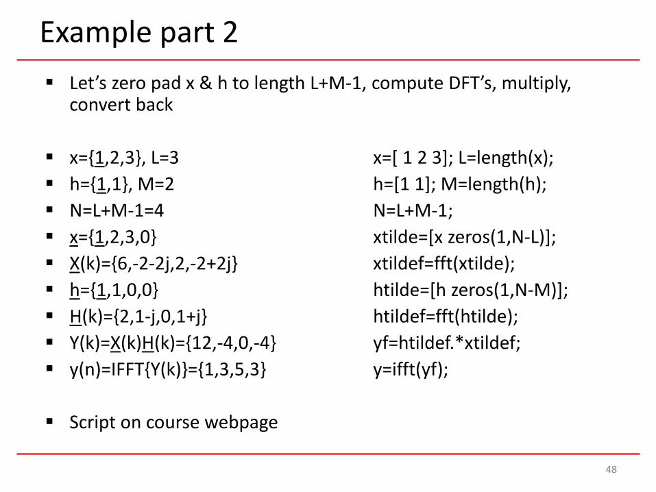
Let’s zero pad x & h to length L+M-1, compute DFT’s, multiply, convert back
x={1,2,3}, L=3 x=[ 1 2 3]; L=length(x); h={1,1}, M=2 h=[1 1]; M=length(h); N=L+M-1=4 N=L+M-1; x={1,2,3,0} xtilde=[x zeros(1,N-L)]; X(k)={6,-2-2j,2,-2+2j} xtildef=fft(xtilde); h={1,1,0,0} htilde=[h zeros(1,N-M)]; H(k)={2,1-j,0,1+j} htildef=fft(htilde); Y(k)=X(k)H(k)={12,-4,0,-4} yf=htildef.*xtildef; y(n)=IFFT{Y(k)}={1,3,5,3} y=ifft(yf);
Script on course webpage

Example done incorrectly
49
Without zero padding, things won’t work x=[1 2 3]; h=[1 1 0]; % same length xf=fft(x); % {6,-1.5+sqrt(3)/2j,-1.5-sqrt(3)/2j} hf=fft(h); % {2,0.5-sqrt(3)/2j,0.5+sqrt(3)/2j} y=ifft(xf.*hf); % {4,3,5}
How did {1,3,5,3} become {4,3,5}?
The last “3” in {1,3,5,3} got folded into “1” at time n=0– mod(3,3)=0– This is aliasing

Filtering Long Sequences

Challenge
51
Reconsider multipath problem Input x contains 100M samples per sec Impractical to do this with 100M
– Need to sample x– Store x– Compute FFT– Multiply with H(k)– IFFT…– And 1 second delay(!)
Plan B: partition x into blocks, compute stuff block by block, then put together (maybe patch between blocks)
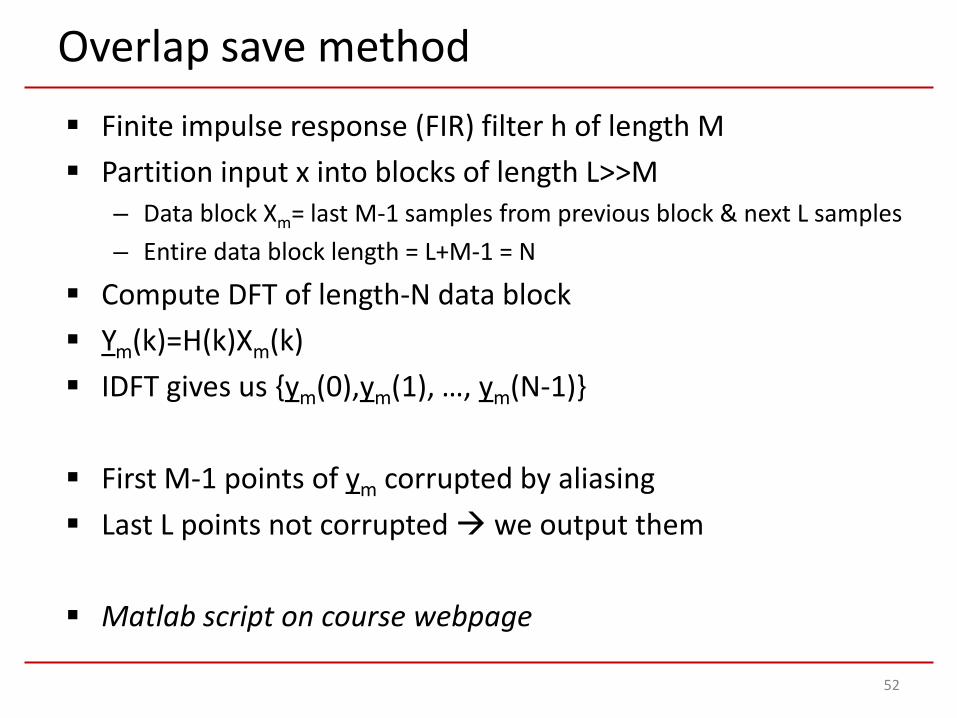
Overlap save method
52
Finite impulse response (FIR) filter h of length M Partition input x into blocks of length L>>M
– Data block Xm= last M-1 samples from previous block & next L samples– Entire data block length = L+M-1 = N
Compute DFT of length-N data block Ym(k)=H(k)Xm(k) IDFT gives us {ym(0),ym(1), …, ym(N-1)}
First M-1 points of ym corrupted by aliasing Last L points not corrupted we output them
Matlab script on course webpage

Overlap add method
53
Prevent aliasing in each block by zero padding End of current output block must be added to beginning of
next output block Details in book
Frequency Analysis Using DFT[Reading material: Sections 7.4-7.5]
Why frequency analysis?
55
Many signals are spectrally sparse
But we don’t know the spectral occupancy will estimate it
Example application– Radio signals (AM/FM) - want to identify carrier frequency – Some include pure sinusoid to aide synchronization
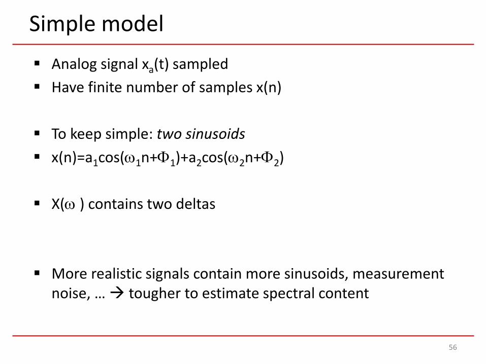
Simple model
56
Analog signal xa(t) sampled Have finite number of samples x(n)
To keep simple: two sinusoids x(n)=a1cos(ω1n+Φ1)+a2cos(ω2n+Φ2)
X(ω ) contains two deltas
More realistic signals contain more sinusoids, measurement noise, … tougher to estimate spectral content

Spectrum of finite duration samples
57
We have finite duration x(n) Can model it as x(n)=x(n)b(n)
𝑏𝑏 𝑛𝑛 = �1, 0 ≤ 𝑛𝑛 ≤ 𝑙𝑙 − 10, 𝑒𝑒𝑙𝑙𝑒𝑒𝑒𝑒
X(ω)=X(ω)*B(ω)– X(ω) contains two deltas– B(ω) Dirichlet kernel (resembles sinc)
ω
X(ω)
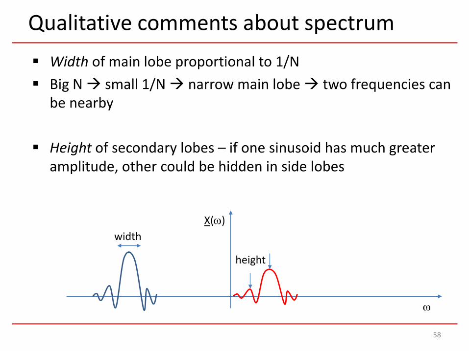
Qualitative comments about spectrum
58
Width of main lobe proportional to 1/N Big N small 1/N narrow main lobe two frequencies can
be nearby
Height of secondary lobes – if one sinusoid has much greater amplitude, other could be hidden in side lobes
ω
X(ω)width
height
Windowing
59
Bad news – even for big N have limits on how well we can separate nearby freqs
Good news – can do better than finite duration signal (convolution w/Dirichlet kernel)– Want to convolve deltas w/narrow main & low side lobes
Windowing – x(n)=x(n)w(n)– w(n) is window– Window has finite duration N– Different trade-offs between main lobe width & side lobe height
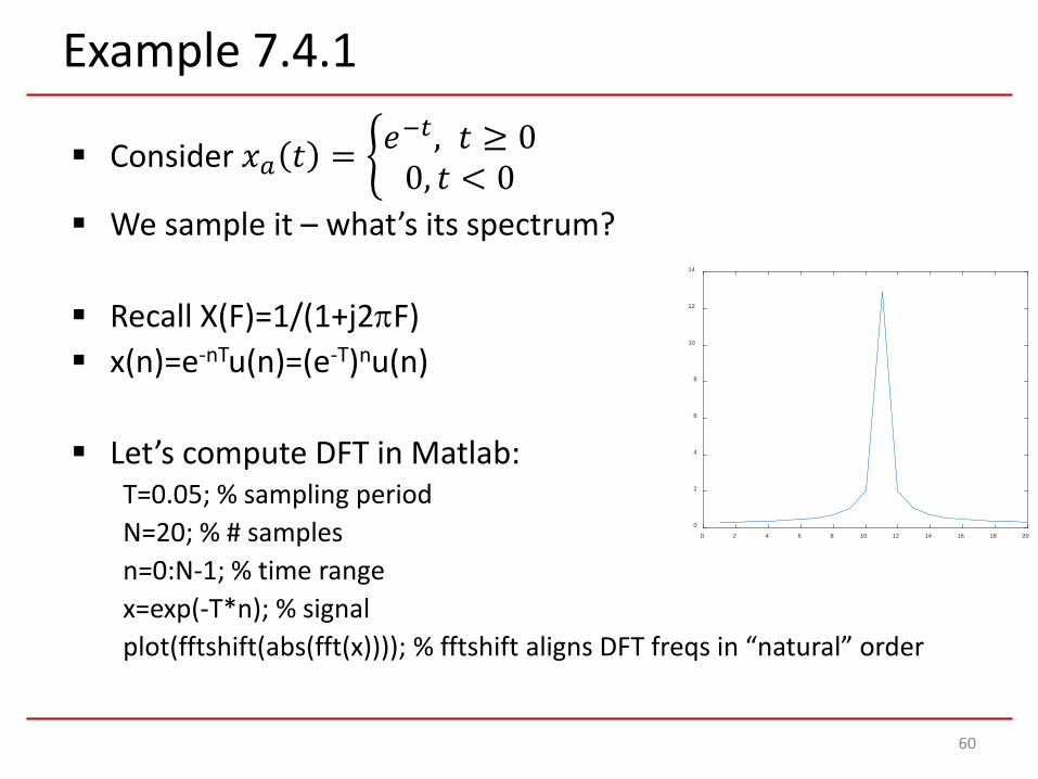
Example 7.4.1
60
Consider 𝑥𝑥𝑎𝑎 𝑡𝑡 = �𝑒𝑒−𝑡𝑡 , 𝑡𝑡 ≥ 00, 𝑡𝑡 < 0
We sample it – what’s its spectrum?
Recall X(F)=1/(1+j2πF) x(n)=e-nTu(n)=(e-T)nu(n)
Let’s compute DFT in Matlab:T=0.05; % sampling periodN=20; % # samplesn=0:N-1; % time rangex=exp(-T*n); % signalplot(fftshift(abs(fft(x)))); % fftshift aligns DFT freqs in “natural” order
0 2 4 6 8 10 12 14 16 18 20
0
2
4
6
8
10
12
14
Example 7.4.1 with bad windowing
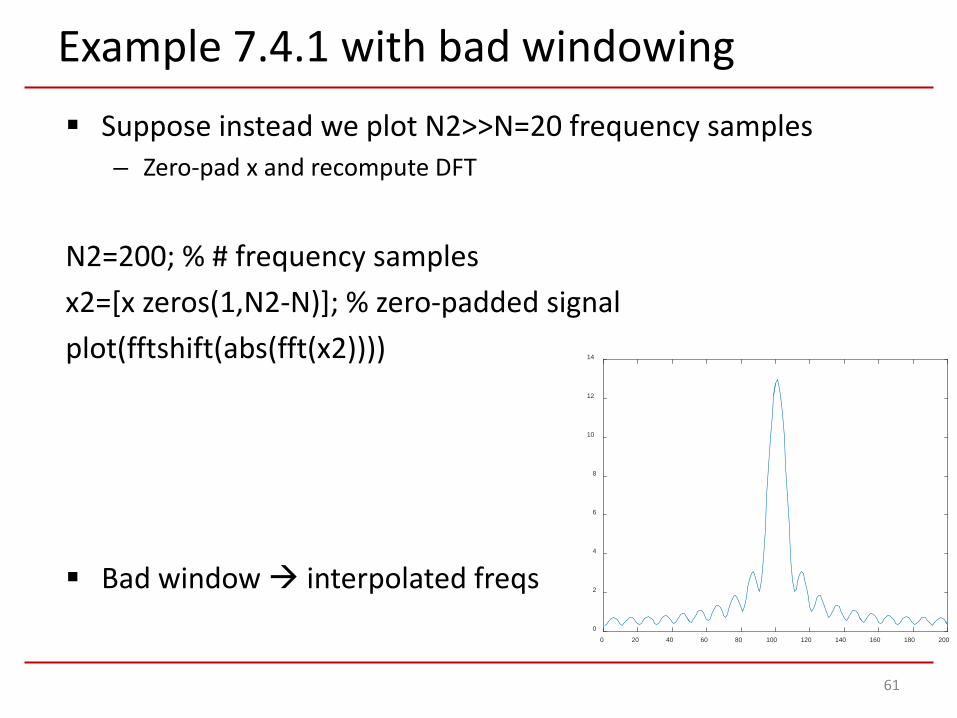
61
Suppose instead we plot N2>>N=20 frequency samples– Zero-pad x and recompute DFT
N2=200; % # frequency samplesx2=[x zeros(1,N2-N)]; % zero-padded signalplot(fftshift(abs(fft(x2))))
Bad window interpolated freqs
0 20 40 60 80 100 120 140 160 180 200
0
2
4
6
8
10
12
14
Discrete Cosine Transform (DCT)
From complex to real valued transforms
63
DFT requires computation with complex arithmetic more time
But most applications have real valued signals
Even (symmetric) real signal has even real transform– Copy signal from time n=1,…,N-1 to negative n– Signal became even real even real-valued transform coeffs– Can compute w/cosines real-valued arithmetic
Advantages of DCT– Algorithms for fast computation (resemble FFT)– Energy compaction properties (DCT coeffs are sparse)