ece 350 experiment 1 spring 2013 - university of wisconsin

ECE 350 Experiment 1 Spring 2013

The purpose of this experiment is to become acquainted with the tools installed on your station. Inthis experiment you will use the software packages MATLAB and SIMULINK. These two packagesare among the most popular tools that control engineers use.

Include all the printouts in your report!

1. Run MATLAB and open the Demo window by clicking on Start button (icon in the bottom-left corner), Demos. Go through the demos and get familiar with basic matrix functions thatMATLAB offers.

(a) Generate two random nonsingular 3 × 3 matrices A and B. Compute the inverse of Aand the transpose of A. Print the results.

(b) Using A and B, compute A ∗ B and A. ∗ B. Print the result and explain what is thedifference between the two operations.

(c) Describe what does the function eig() do.

(d) Plot a graph of function f(x) = e−2x sin(3x + 1) on the interval x ∈ [0, 10].

2. Explore Simulink by clicking on Start→ Simulink→ Demos. You can find lots of informationin the video demos.

3. In the Simulink Demos window, scroll to General Applications (or use the explorer windowon the left) and open Thermal Model of a House demo. Open the model and this will starta demo of the thermodynamics of a house in SIMULINK. Explore the demo by clicking ondifferent blocks.

(a) Double click on the Scope block labeled PlotResults. Start the simulation by using Startcommand on the Simulation menu, or by clicking the Play button. Let the simulationrun for some time and then stop the simulation by choosing Stop. Print the plots andexplain what they represent.

(b) The constant block labeled Set Point sets the desired temperature. Change the value to80F. Run the simulation again and see how the indoor temperature and the heating costchanges. Print the results.

(c) Adjust the daily temperature variation by opening the Sine Wave block labeled DailyTemp Variation and changing the Amplitude parameter. Repeat the simulation, printthe results and comment what happened.

4. Now we want to build a simple model in SIMULINK. We would like to integrate a sine waveand display the result along with the sine wave.

Open a new model in Simulink. To create the model you will need to copy blocks into themodel from the following SIMULINK block libraries:

• Sources library (the Sine Wave block).

1

• Sinks library (the Scope block).

• Continuous library (the Integrator block).

• Signals & Systems library (the Mux block).

Find all these blocks and drag the appropriate icons into the Model window. You will seethat the icons have little > parts. These represent input and output ports.

Connect the output of the Sine Wave block with the top input of the Mux block (click theleft mouse button on the appropriate port and while pressing the button move to the portyou want connected). Similarly, connect the output of the Integrator and the bottom inputof the Mux, and the output of the Mux and the input of the Scope. Now we would also liketo connect the output of Sine Wave with the input of the Integrator. To do this:

(a) Position the pointer on the line connecting Sine Wave with the Mux.

(b) Press and hold down the Ctrl key (or click the right mouse button) and drag the line tothe input of the Integrator.

(c) Release the button.

Print out the drawing of the model when you are done.

Now open the Scope block to view the simulation output. Set SIMULINK to run for 10seconds by adjusting Stop time in the box Simulation Parameters under the Simulationmenu.

Start the simulation and watch the traces on the Scope. Print the results and explain whatthe curves represent.

Save the model by choosing Save from the File menu. Exit MATLAB.

2


Transfer functions are a convenient and powerful way to model systems. Most transfer functionsare rational functions – quotients of polynomials.

The objective of this experiment is twofold:

• To learn how to use MATLAB to: (1) generate polynomials; (2) manipulate polynomials; (3)generate transfer functions; (4) manipulate transfer functions; and (5) perform partial-fractionexpansions.

• To learn to use MATLAB and the Symbolic Toolbox to: (1) find Laplace transforms fortime functions; (2) find time functions from Laplace transforms; (3) create LTI transfer func-tions from symbolic transfer functions; and (4) perform solutions of symbolic simultaneousequations.

Include all the printouts in your report!

1 Polynomials

You can find a quick tutorial on basic operations with polynomials in Matlab at http://www.

matrixlab-examples.com/polynomials.html and another one at http://www.engin.umich.edu/group/ctm/basic/basic.html#polynomial.

1. Using Matlab, compute:

(a) The roots of P1 = s6 − 8s5 + 4s4 + 82s3 − 125s2 − 74s + 120.

(b) The roots of P2 = s5 − 2s4 + s3 + 2s2 − 2s.

(c) P3 = P1 + P2; P4 = P1 − P2; P5 = P1P2; P6 = P1/P2.

2. Find a Matlab command that can compute the coefficients of the polynomial:

P7 = (s + 3)(s− 2)(s + 1)(s + 5)(s− 6)(s + 7).

2 Transfer Functions

A nice tutorial on how to use Matlab for transfer function operations can be found at http://www.regpro.jku.at/downloads/autpr/Tutorials/MatlabSimulink/DefiningTransferFunctionsinMatlab.

htm. You can also obtain help on a Matlab command by using “doc command ”.

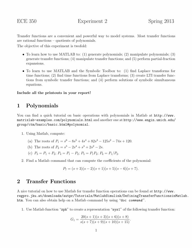
1. Use Matlab function “zpk” to create a representation “sys1” of the following transfer function:

G1 =20(s + 1)(s + 3)(s + 6)(s + 8)

s(s + 7)(s + 9)(s + 10)(s + 15).

1

http://www.matrixlab-examples.com/polynomials.html

http://www.matrixlab-examples.com/polynomials.html

http://www.engin.umich.edu/group/ctm/basic/basic.html#polynomial

http://www.engin.umich.edu/group/ctm/basic/basic.html#polynomial

http://www.regpro.jku.at/downloads/autpr/Tutorials/MatlabSimulink/Defining Transfer Functions in Matlab.htm



Apply the function “tf” to “sys1′′ to find G1 represented as a numerator polynomial dividedby a denominator polynomial.

2. Now find how the transfer function

G2 =s4 + 17s3 + 99s2 + 223s + 140

s5 + 32s4 + 363s3 + 2092s2 + 5052s + 4320,

can be represented as a product of factors in the numerator divided by a product of factorsin the denominator.

3. Compute G3 = G1 + G2, G4 = G1 −G2 and G5 = G1G2, and represent the results as factorsdivided by factors, and as polynomials divided by polynomials. Do G1 and G2 need to beexpressed in the same form to perform these operations?

4. Use the function “residue” and compute partial-fraction expansion of the following transferfunctions:

(a) G6 = 5(s+2)s(s2+8s+15)

,

(b) G7 = 5(s+2)s(s2+6s+9)

,

(c) G8 = 5(s+2)s(s2+6s+34)

.

3 System Models

For this part, you might want to go over tutorials for the Matlab Symbolic Toolbox. The followingMatlab functions will be useful for the problems: “poly2sym”, “sym2poly”, “numden”, “tfdata”,“laplace”, “ilaplace”, and “solve”.

1. Define a symbolic function

f(t) =5 (cos(2 t) + 5 sin(2 t))

8 e3 t− 5

8 et,

and compute its Laplace transform.

2. Define a symbolic function

F (s) =2(s + 3)(s + 5)(s + 7)

s(s + 8)(s2 + 10s + 100),

and find its inverse Laplace transform. Also generate a transfer function model correspondingto F (s) both as factors divided by factors, and as polynomials divided by polynomials.

3. Using Symbolic Toolbox in Matlab, find the three loop currents for the following circuit:

2


Many engineering systems exhibit nonlinear behavior. Since there are many more tools available todesign and study linear systems than nonlinear systems, it is customary to approximate a nonlinearsystem with its linearization around an operating point. In this experiment you will use Matlaband Simulink to compare the behavior of a nonlinear system with its linearization.

1. Consider a pendulum, that is a point mass m swinging on a massless rod of length l:

lϕ

m

gravity

Figure 1: A pendulum.

(a) Derive the differential equation in ϕ describing the motion of the mass m. Now introducethe following two variables:

x1 = ϕ

x2 = ϕ

We clearly have the relation x1 = x2. Determine the expression for x2 using the differ-ential equation you derived before.

Let x =

[x1

x2

]. You can write the equations for the pendulum in the form:

x = f(x)

where f(x) is a 2 × 1 vector function. Determine the function f(x). The model in thisform is called a state space model.

(b) If you performed the calculations correctly, the function f(x) should be nonlinear. Writea first order Taylor series of f(x) around the point x1 = 0, x2 = 0. Recall that a Taylorseries of a function of x = (x1, x2, . . . , xn) around the point x0 = (x0

1, x02, . . . , x

0n) is:

f(x1, x2, . . . , xn) ≈ f(x0)+∂f

∂x1

|x=x0(x1−x01)+

∂f

∂x2

|x=x0(x2−x02)+· · ·+ ∂f

∂xn

|x=x0(xn−x0n)

1

Using the Taylor series, you can write a linearized model of the pendulum in the form:

x = Ax

where A is a constant 2× 2 matrix. Determine A.

(c) We would like to build a simulation of the pendulum in Simulink. Schematically, asimulation of the system described with a state-space model looks like Figure 2.

Figure 2: Block diagram for the simulation.

Use two integrators for x1 and x2 and combine the signals using elements from the Mathlibrary to build the model of the pendulum in Simulink. For the simulation, use thevalues m = 1kg and l = 1m. In the same Simulink window, build the model of thelinearized system. Using the Scope block and the Mux block, display the x1 variablefor the pendulum and for the linearized system.

(d) We would like to compare how well does the linearized system describe the pendulum.First, you will need to set the initial conditions for the simulation by setting the initialconditions of the integrators. To do that, click on the Integrator block, specify theInitial condition source as internal and enter the value in the Initial conditionparameter field.

Run the simulation for 10s for the initial conditions:

i. x1 = 5, x2 = 0.

ii. x1 = 10, x2 = 0.

iii. x1 = 30, x2 = 0.

iv. x1 = 50, x2 = 0.

Print the results in each case. What can you say about the relation between the behaviorof the pendulum and that of the linearized system?

2


One of the most important components of a control system is the actuator. Many systems rely onan electrical actuator, and among these, DC motor continues to be the most popular choice. Inthis experiment you will explore the behavior of a DC motor and learn how it is used in controlsystems.

Remember to save all your work on portable media.

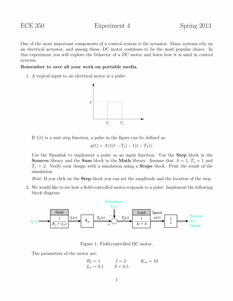
1. A typical input to an electrical motor is a pulse:

A

Ts Tf

If 1(t) is a unit step function, a pulse in the figure can be defined as:

p(t) = A (1(t− Ts) − 1(t− Tf )) .

Use the Simulink to implement a pulse as an input function. Use the Step block in theSources library and the Sum block in the Math library. Assume that A = 1, Ts = 1 andTf = 2. Verify your design with a simulation using a Scope block. Print the result of thesimulation.

Hint: If you click on the Step block you can set the amplitude and the location of the step.

2. We would like to see how a field-controlled motor responds to a pulse. Implement the followingblock diagram:

Tm(s)If (s)Vf (s) s

11

R f L f s

Disturbance

Td (s)

TL(s)

Speed

v (s) Position

u (s)

Output

Field

1

Js b

Load

Km

FIGURE 2.19

Block diagram model of field-controlled dc motor.

Dorf/Bishop

Modern Control Systems 9/E

© 2000 by Prentice Hall, Upper Saddle River, NJ.

Figure 1: Field-controlled DC motor.

The parameters of the motor are:

Rf = 1 J = 2 Km = 10Lf = 0.1 b = 0.5

1

(a) Use the Transfer Fcn block in the Continuous library to implement each transferfunction. You can change the coefficients of the transfer function by clicking on theblock.

Let the input Vf be the pulse you implemented above. Set the disturbance to be aConstant block in the Sources library. Set the value of the constant to 0.

(b) Using the Mux block, connect the output of the motor θ, the torque Tm and the inputVf to a scope. Set the Stop time for the simulation to 40. Open the scope window andrun the simulation. Click the right button on the scope window to Autoscale the plot.Print the result.

(c) Now set the value of the disturbance torque Td to 0.1. Run the simulation again, Au-toscale the plot and print the result. Comment on the difference from the previoussimulation.

3. We would like to compare the performance of the field-controlled motor with that of anarmature-controlled motor:

Tm(s)Va(s)

Js b

1s1Km

Ra Las

Kb

Disturbance

Td (s)

TL(s)

Speed

v (s) Position

u (s)

Back emf

Armature

FIGURE 2.20

Armature-controlled dc motor.

Dorf/Bishop



Figure 2: Armature-controlled DC motor.

(a) For the same parameters as above and assuming Ra = Rf , La = Lf , Kb = Km, draw theblock diagram of the armature-controlled motor in Simulink. Use the pulse for the inputand 0 for the disturbance torque Td.

(b) Using the Mux block, connect the output of the motor θ, the torque Tm and the inputVa to a scope. Set the Stop time for the simulation to 40. Open the scope window andrun the simulation. Click the right button on the scope window to Autoscale the plot.Print the result.

(c) Compare the performance of the armature-controlled motor with that of the field-controlledmotor. In particular, comment on the torque response, Tm. Based on the shape of Tm,which configuration seems simpler to use?

2


In this exercise you will see how signal-flow graphs and Mason’s formula can be used to analyze afunction of a transistor. This way of modeling can be considered an alternative to standard circuitanalysis.

The following figure shows the small signal circuit representation of a common-emitter transistoramplifier:

1. Draw a signal-flow graph representation of the circuit. Use the following nodes:

vin vbe vceib if ic

and the following nodal equations:

ib =vin − vbeRs

+ if

if =vce − vbeRf

ic =vcehoe

+ βib

vbe = hrevce + hieib

vce = −(if + ic)RL

2. Using Mason’s formula determine the transfer function between vin and vce.

3. Represent the signal-flow graph with a block diagram in Simulink. Do not use numericalvalues, use variables to represent the transfer functions (i.e., use 1/Rf instead of 0.1 even ifyou know that Rf = 10). Print the block diagram. Use the Signal Generator from theSources library as the input vin.

1

4. In Matlab, create an M-file and define the following variables (use the names you used inSimulink):

Rs = 1Ω Rf = 100Ω RL = 10kΩhre = 0.1 hoe = 50Ω hie = 2kΩβ = 1500

Run the simulation when vin is a sawtooth waveform with the amplitude 5V and frequency10Hz. Plot vin, vce, and vce

vin. How can you check whether your derived transfer function is

correct?

2


Signal-flow graphs are a good way to simulate a transfer function. In this exercise you will learnhow to implement signal-flow graphs in Simulink and use them to study system response.

1. Find a signal-flow graph that corresponds to the controller canonical form (phase-variablecanonical form) realization of the following transfer function:

T (s) =s + 2

(s− 3)(s2 + 2s + 2)

Write also the matrices that describe this system in the state-space form.

2. Using the ss function in Matlab define the state space model of the system. Use the tf

function to convert the state-space representation into a transfer function and verify thatyour state space model corresponds to the transfer function T (s).

3. Implement the signal-flow graph above in Simulink. Plot the response of the system to theunit step input. What can you say about this system?

4. To improve the performance of the system we can design a feedback controller. If u(t) isthe input signal and x is the state, the so-called state feedback controller is described byequation:

u = v −Kx

where v is the new input and K is a 1× 3 vector called the gain vector. Modify the signal-flow graph above to implement a state feedback controller and plot the step response of theresulting system for:

(a) K = [8 8 4]

(b) K = [5 5 3]

(c) K = [12 14 6]

5. Based on your analysis, suggest the best controller for the system.

Print all the plots and submit them with your report.

1


Open and closed loop systems respond in different ways to disturbances and effects of unmodeleddynamics. In this exercise you will compare open and closed systems using Matlab and Simulink.The purpose of the exercise is to show you how having numerical tools allows a designer to quicklyevaluate different design alternatives.

A remotely controlled vehicle has the transfer function:

G(s) =1

s2 + 2s + 4

We want to compare an open loop controller with a closed loop controller.

1. Design a proportional open loop controller:

H(s) = K.

Figure 1 shows the diagram of the overall system. On the figure, R(s) is the input and D(s)is a disturbance.

GHYR

D

+

−

Figure 1

(a) Plot the response of the system to a step input (assuming D(s) = 0) for K = 1, 4, 10.How does a change in K affect the response? Which K would you choose to get asteady-state error equal to zero?

(b) Plot the response of the system to a unit step disturbance (assuming R(s) = 0). Evaluatethe steady-state error for a disturbance numerically (from the plot) and analytically. DoesK affect the disturbance response of the system?

(c) What is the sensitivity of the open-loop transfer function to changes in K?

2. Now design a closed-loop controller:

H(s) =K(s + 2)

(s + 1).

The overall system is shown in Figure 2.

1

H G+−

R Y

D

+−

Figure 2

(a) Plot the response of the system to a step input (assuming D(s) = 0) for K = 4.5, 10, 20.Create a table and compare the three responses with respect to the:

• The time at which the response reaches its peak.

• The steady-state error.

• Percentage the system overshoots the steady-state value. Compute this value asMp−Fs

Fswhere Mp is the peak value and Fs is the steady-state value.

Which K would you choose for the system based on your table?

(b) Plot the response of the system to a unit step disturbance (assuming R(s) = 0) for thesame values of K. In each case, determine the steady-state error of the system. WhichK gives the smallest error?

(c) Evaluate the sensitivity of the closed-loop transfer function to changes in K. Using thenominal value K = 10, plot a graph of the sensitivity function on the complex plane forfrequencies ω = 0.01rad/s to ω = 100rad/s.

Hint: Figure 4.33 in Dorf & Bishop shows you how to do this.

3. Based on your analysis, suggest the best design for the system.

Print all the plots and submit them with your report.

2


In this exercise you will explore a typical response of first and second order systems. All othersystems can be usually approximated with first or second order systems so it is important to bewell acquainted with these typical responses.

1. Consider the first order system:

G(s) =p

s+ p

where p is a parameter. On the same figure, plot the step response of the system for p = 1, 2, 10.How does p affect the response?

2. Now consider a second order system:

G(s) =K

s2 + ps+K

where K and p are the parameters of the system.

(a) For K = 1, plot the step response of the system for p = 0, 1, 2, 5. Plot all the responseson the same figure! Comment on the effect of p on the response. On one figure, sketchthe location of the poles of the system in the complex plane for each value of p (you canuse the function pzmap to find the location of the poles).

(b) On one figure, plot the step response of the system for K = 1, 2, 10 and p = 0.8K. Howdoes the response change in this case? Sketch the location of the poles of the system inthe complex plane for each value of K on one figure.

3. Now consider a second order system with a zero:

G(s) =(γs+ 1)

s2 + 1.2s+ 1

On the same figure, plot the step response of the system for γ = 0, 0.1, 1, 10. Note that γ = 0corresponds to the case when the system has no zeros. Identify the location of the zero foreach value of γ. On one figure, sketch the location of the poles and the zero for each value ofγ. How does a zero affect the response of a second order system?

4. Consider the third order system:

G(s) =1

(s2 + s+ 1)(γs+ 1)

On the same figure, plot the step response of the system for γ = 0, 0.05, 0.1, 1, 10. Note thatγ = 0 corresponds to the case when the system has no additional pole. Identify the locationof the pole for each value of γ and sketch the location of all the poles on the complex plane(again, do this on one figure). How does a third pole affect the response of a second ordersystem?

1

ECE 350 Laboratory 9 Spring 2013

High order systems can be usually well approximated as a first or a second order system. This isimportant for design of controllers since it significantly simplifies the problem. However, care needsto be taken with approximation so that all the important properties of the system are preserved.This exercise will introduce you to some of these issues.

1. Consider the system:

G(s) =15

(s2 + 2s + 2)(s + 8)

(a) Plot the step response of the system. Determine the percent overshoot, the peak time,and the steady-step error for the step response.

(b) We would like to approximate the system with a second-order system

G(s) =K

s2 + 2s + 2.

Determine the value K that will result in the same steady-state error as the originalsystem. Plot the step response of G for this value of K. Determine the percent overshoot,the peak time and the steady-state error and compare them with those of the originalsystem. What can you say about this approximation?

2. Consider the system:

G(s) =0.1(s + 8)

(s2 + 1.5s + 1)

(a) Plot the step response of the system. Determine the percent overshoot, the peak time,and the steady-step error.

(b) We would like to approximate the system with a system without a zero:

G(s) =K

s2 + 1.5s + 1.

Determine the value K that will result in the same steady-state error as the originalsystem. Plot the step response of G for this value of K. Determine the percent overshoot,the peak time and the steady-state error and compare them with those of the originalsystem. What can you say about this approximation?

3. Now consider the following system:

G(s) =12(s + 4)

(s2 + 3s + 4)(s + 12)

Find a second order system that best approximates this system and has the minimal number ofzeros. Explain how you arrived at your solution and provide plots that support your decision.

1


Stability is the most important property that a closed-loop system should posses. The first step inthe design of a control system is thus to identify the values of the parameters for which the systemis stable. Within the region of stability, the parameters can be subsequently adjusted for optimalperformance. The purpose of this exercise is to introduce you to this two-level process. Note thatthere are typically many choices of the parameter values that will achieve the desiredperformance.

1. An automatically guided vehicle on Mars is represented by the following system:

R(s)

Steering

command

Y(s)

Direction of

travel

H(s)

10

s 10

1

s2

FIGURE DP6.2

Mars guided vehicle control.

Dorf/Bishop



The system has a steerable wheel in both the front and back of the vehicle, and the designrequires that H(s) = Ks + 1. Determine

(a) The value of K required for stability.

(b) The value of K when one root of the characteristic equation is equal to s = −5.

(c) The value of the two remaining roots for the gain selected in (b).

(d) Find the step response for the gain selected in part (b).

2. The following figure shows the attitude control system of a space shuttle rocket:

(s m)(s 2)

sR(s)

Y(s)

Attitude

Space shuttle

rocket

K

s2 1

Controller

FIGURE DP6.4

Shuttle attitude control.

Dorf/Bishop



(a) Determine the range of gain K and parameter m so that the system is stable. Plot theregion of stability on the K vs. m plot.

(b) Select the gain and parameter values so that the steady-state error to a ramp input isless than or equal to 10% of the input magnitude.

(c) Determine the percent overshoot for a step input for the system selected in part (b).

1


Design of controllers is usually an iterative process. A controller is typically designed for an ap-proximation of the system. Subsequently, it is applied to the full system and refined until all thespecifications are met. In this exercise you will go over these steps. Note that there are typicallymany choices of the parameter values that will achieve the desired performance.

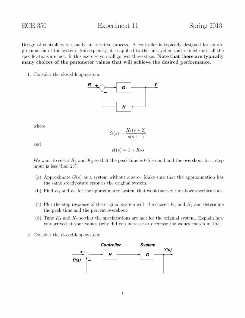
1. Consider the closed-loop system:

+

H

G−

R Y

where

G(s) =K1(s + 2)

s(s + 1),

andH(s) = 1 + K2s.

We want to select K1 and K2 so that the peak time is 0.5 second and the overshoot for a stepinput is less than 2%.

(a) Approximate G(s) as a system without a zero. Make sure that the approximation hasthe same steady-state error as the original system.

(b) Find K1 and K2 for the approximated system that would satisfy the above specifications.

(c) Plot the step response of the original system with the chosen K1 and K2 and determinethe peak time and the percent overshoot.

(d) Tune K1 and K2 so that the specifications are met for the original system. Explain howyou arrived at your values (why did you increase or decrease the values chosen in 1b).


H G−

+ Y(s)

R(s)

Controller System

1

where

G(s) =10

(s + 1)(s + 9),

and

H(s) =K

s + 90.

(a) Determine a second-order model for the closed-loop system by approximating H(s) withits DC gain (the steady-state value of the step response).

(b) Using the second-order model, select a gain K so that percent overshoot is less than 15%and the steady-state error to a step is less than 12%.

(c) Verify your design by determining the actual performance of the third-order system(submit the step response plot with your report).

(d) Tune the value of K so that the specifications are met. Plot the step response of thesystem to show that your design works. Explain how you arrived at your new value.

2


The Root Locus procedure was derived to help in the design of control systems. Matlab providestwo functions for working with root locus: rlocus and rlocfind. The first sketches the root locuswhile the second enables the user to find the value of the parameter at a particular point on theroot locus. But although one might be tempted to completely rely on the Matlab to draw the rootlocus, it is important to understand the steps that are involved in drawing an approximate rootlocus in order to effectively use it for control system design.

1. Using Matlab’s Help system, read about the functions rlocus and rlocfind.


+

H

G−

R Y

where

G(s) =s(3s2 + 5s− 20)

(s2 − 2s + 10)(s + 3)(s + K)

andH(s) = 1.

(a) Find the characteristic polynomial of the closed-loop system.

(b) Transform the characteristic polynomial into the root-locus form.

(c) Plot the root locus for the parameter K using Matlab.

(d) Using rlocfind find the value of K and the location of the roots where the root-locusbreaks off from the real axis.

(e) Find the value of K and the location of the roots where the root-locus merges to the realaxis.

(f) Find the value of K at which the system becomes unstable. Identify all the roots of thecharacteristic equation for this value of K.

1

3. Root locus is especially useful in design of controllers. Consider the following configuration:

H G−

+ Y(s)

R(s)

Controller System

where the system transfer function is

G(s) =s + 1

(s + 3)(s− 1)(s− 2)

and H(s) is a controller.

(a) Let H(s) = K. This is a so-called proportional controller. Using Matlab, plot the rootlocus for K. Can you stabilize the system using this controller?

(b) Now consider the controller in the form:

H(s) = K1 +K2

s+ K3s. (1)

This is so-called PID controller. In order to effectively use the root locus for designingthe PID controller, we can represent the PID controller in the form:

H(s) = K(s + z1)(s + z2)

s(2)

i. Find the relation between the location of the zeros z1 and z2 in Equation (2) andthe parameters K1, K2, and K3 in Equation (1).

ii. Place the zeros of the controller at −2 ± 3j (that is, z1,2 = 2 ∓ 3j). Plot the rootlocus of the system for K (using the form of H(s) in Equation (2)). What can yousay about the ability of this controller to stabilize the system?

iii. For the PID controller above, find the value of K for which the system’s complexconjugate poles have their real part equal to −1. For this value of K, identify whatare the corresponding parameters K1, K2, and K3 in Equation (1).

2


PID controllers are widely used in industrial process control due to their good performance in awide range of operating conditions and their functional simplicity. In this exercise you will explorehow the PID controllers can be designed using the root locus procedure.

You are encouraged to take the advantage of the Matlab functions rlocus and rlocfind for thisexercise.

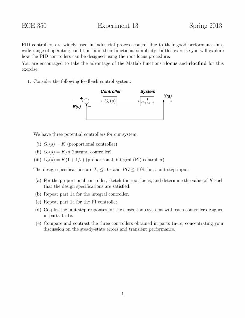
1. Consider the following feedback control system:

−

+ Y(s)

R(s)

Controller System

Gc(s)1

s2+5s+6

We have three potential controllers for our system:

(i) Gc(s) = K (proportional controller)

(ii) Gc(s) = K/s (integral controller)

(iii) Gc(s) = K(1 + 1/s) (proportional, integral (PI) controller)

The design specifications are Ts ≤ 10s and PO ≤ 10% for a unit step input.

(a) For the proportional controller, sketch the root locus, and determine the value of K suchthat the design specifications are satisfied.

(b) Repeat part 1a for the integral controller.

(c) Repeat part 1a for the PI controller.

(d) Co-plot the unit step responses for the closed-loop systems with each controller designedin parts 1a-1c.

(e) Compare and contrast the three controllers obtained in parts 1a-1c, concentrating yourdiscussion on the steady-state errors and transient performance.

1

2. Consider the spacecraft single-axis attitude control system:

−

+ Y(s)

R(s)

PD Controller Spacecraft

K1 +K2s 1

Js2

The controller is known as proportional-derivative (PD) controller.

(a) Sketch the root locus for K1 when K2 = 0.

(b) Suppose that we require the ratio of K1/K2 = 5. Sketch the root locus for the systemand discuss how it differs from the previous case.

(c) Using the root locus, find the values of K2/J and K1/J in part (b) such that Ts ≤ 4sand PO ≤ 10% for a unit step input.

2


This laboratory exercise is optional. If you hand it in you will receive extra credit.

Control Toolbox in Matlab provides a powerful tool for helping with the design of the controlsystems called “sisotool”. You can read about the tool at http://www.mathworks.com/help/

toolbox/control/getstart/f2-1037701.html. In this exercise you will use “sisotool” to solvetwo problems requiring design of controllers.

Before using “sisotool”, define systems in the main Matlab window. You can then import thesesystems directly into “sisotool” as explained in the tutorial (click Architecture → SystemData in “sistool” window). For example, to define the transfer function:

G1(s) =1

(s + 2)(s + 4)(s + 6)(s + 8)

you can either use

g1=zpk([],[-2 -4 -6 -8],1)

or

s=tf('s');

g1=1/((s+2)*(s+4)*(s+6)*(s+8))

Use “sisotool” to solve the following problems:

1. Take a unity feedback system with

G(s) =K

(s + 2)(s + 4)(s + 6)(s + 8).

First, find K so that the uncompensated system will have a damping ratio of 0.5. Thenfind the transfer function of a lead-lag compensator that will yield a settling time 0.5 secondshorter than that of the uncompensated system, will also result in the damping ratio of 0.5,and will improve the steady-state error by a factor of 30. The compensator zero should beat −5. Find the compensated system’s gain. Justify any second-order approximations andverify the design through simulation.

2. Take a unity feedback system with

G(s) =K

(s + 1)(s + 4).

1

http://www.mathworks.com/help/toolbox/control/getstart/f2-1037701.html

http://www.mathworks.com/help/toolbox/control/getstart/f2-1037701.html

Design a PID controller that will yield a peak time of 1.047 seconds and a damping ratio of0.8, with zero error for a step input. Remember that you can rewrite the PID controller as:

Kp +Ki

s+ Kds = Kc

(s + z1)(s + z2)

s.

One zero and the pole of the compensator can be then designed as a PI compensator, whilethe other zero can be designed as a PD compensator.

2

ece 350 experiment 1 spring 2013 - university of wisconsin

Documents