ece 302 spring 2012 ilya pollak
TRANSCRIPT

ECE 302 Spring 2012
Practice problems: Continuous random variables; uniform, exponential, normal, lognormal,
Rayleigh, Cauchy, Pareto, Gaussian mixture, Erlang, and Laplace random variables;
quantization; optimal portfolios; simulating a fair coin with a biased one; dependence and
correlation; binary detection.
Ilya Pollak
These problems have been constructed over many years, using many different sources.If you find that some problem or solution is incorrectly attributed, please let me knowat [email protected].
Suggested reading: Sections 3.1-3.7, 4.2, and 4.3 in the recommended text [1]. Equiva-lently, Sections 3.1-3.6, 4.1-4.5, 4.7 (correlation and covariance only) in the Leon-Garciatext [3].
Problem 1. X is a continuous random variable, uniformly distributed between 10 and 12. Find theCDF, the PDF, the mean, the variance, and the standard deviation of the random variable Y = X2.
Solution. Since X is between 10 and 12 with probability 1, it follows that Y = X2 is between 100and 144 with probability 1. Hence, the CDF of Y is zero for all outcomes below 100 and one for alloutcomes above 144. Between 100 and 144, we have:
FY (y) = P(Y ≤ y) = P(X2 ≤ y) = P(X ≤ √y) = FX(
√y) =
√y − 10
2,
where we used the fact derived in class that for x ∈ [10, 12],
FX(x) =x − 10
12 − 10.
The answer for the CDF of Y :
FY (y) =
0, y ≤ 100√y−102 , 100 ≤ y ≤ 144
1, y ≥ 144.
The PDF of Y is obtained by differentiating the CDF:
fY (y) =
0, y ≤ 101
4√
y 100 ≤ y ≤ 144
0, y ≥ 144.
The mean and the variance of Y can be computed either using the PDF of X or using the newlycomputed PDF of Y . As derived in class, the mean and variance of X are 11 and 1/3, respectively.This means that E[Y ] = E[X2] = var(X) + (E[X])2 = 1211
3 . Another way of obtaining the sameresult is through defining a new random variable
S =X − 11
2.
1

Then S is uniformly distributed between -1/2 and 1/2, and has mean zero, as shown in class. It wasalso shown in class that E[S2] = 1/12. Since X = 2S + 11, we have:
Y = X2 = 4S2 + 44S + 121,
and
E[Y ] = E[X2] = 4E[S2] + 44E[S] + 121 = 1211
3.
We can also obtain the same result by using the PDF of Y :
E[Y ] =
∫ 144
100y
1
4√
ydy
=
∫ 144
100
√y
4dy
=y3/2
6
∣∣∣∣∣
144
100
=1728 − 1000
6=
364
3= 121
1
3.
To compute the variance of Y , we can use the formula var(Y ) = E[Y 2]− (E[Y ])2. In order to use thisformula, we need to compute E[Y 2] first. We can do this using the PDF of Y :
E[Y 2] =
∫ 144
100y2 1
4√
ydy
=
∫ 144
100
y3/2
4dy
=y5/2
10
∣∣∣∣∣
144
100
=125 − 105
10=
248832 − 100000
10=
74416
5= 14883.2
Alternatively, we can use the PDF of X to obtain the same result:
E[Y 2] = E[X4] =
∫ 12
10
x4
2dx
=x5
10
∣∣∣∣
12
10
=125 − 105
10= 14883.2
Now we can compute the variance of Y :
var(Y ) = E[Y 2] − (E[Y ])2 =74416
5−(
364
3
)2
=74416 · 9 − 3642 · 5
45=
669744 − 662480
45
=7264
45≈ 161.4
2
α x
) ( x f X
α x
) ( x F X
1
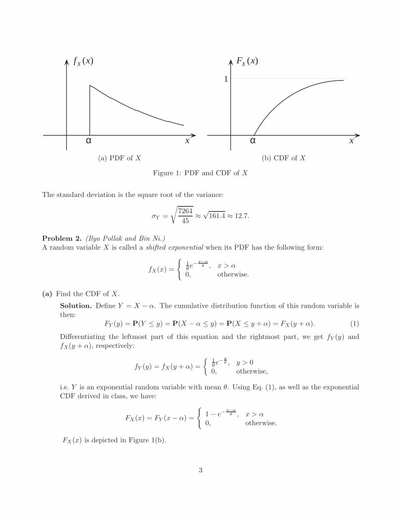
(a) PDF of X (b) CDF of X
Figure 1: PDF and CDF of X
The standard deviation is the square root of the variance:
σY =
√
7264
45≈
√161.4 ≈ 12.7.
Problem 2. (Ilya Pollak and Bin Ni.)A random variable X is called a shifted exponential when its PDF has the following form:
fX(x) =
{1θe−
x−αθ , x > α
0, otherwise.
(a) Find the CDF of X.
Solution. Define Y = X − α. The cumulative distribution function of this random variable isthen:
FY (y) = P(Y ≤ y) = P(X − α ≤ y) = P(X ≤ y + α) = FX(y + α). (1)
Differentiating the leftmost part of this equation and the rightmost part, we get fY (y) andfX(y + α), respectively:
fY (y) = fX(y + α) =
{1θe−
yθ , y > 0
0, otherwise,
i.e. Y is an exponential random variable with mean θ. Using Eq. (1), as well as the exponentialCDF derived in class, we have:
FX(x) = FY (x − α) =
{
1 − e−x−α
θ , x > α0, otherwise.
FX(x) is depicted in Figure 1(b).
3

(b) Calculate the mean and the variance of X.
Solution. It was derived in class that the mean and variance of the exponential random variableY we defined in the last part are θ and θ2 respectively. Since α is just a constant, we have:
E[X] = E[Y + α] = E[Y ] + α = θ + α
V ar[X] = V ar[Y + α] = V ar[Y ] = θ2
(c) Find the real number µ that satisfies: FX(µ) = 1/2. This number µ is called the median of therandom variable X.
Solution. With the CDF we got in Part(a), we have:
1 − e−µ−α
θ =1
2
⇒ µ − α
θ= ln 2
⇒ µ = θ ln 2 + α.
Problem 3. Lognormal random variable, its PDF, mean, and median. (Ilya Pollak).Suppose Y is a normal random variable with mean µ and standard deviation σ. Let X = eY . X iscalled a lognormal random variable since its log is a normal random variable.
(a) Find the PDF and the expectation of X.
(b) The median of a continuous random variable Z is defined as such number d that P(Z ≤ d) =P(Z ≥ d) = 1/2. Find the median of X.
(c) Lognormal random variables are widely used in finance and economics to model compoundedreturns of various assets. Suppose Sk and Sn are the prices of a financial instrument on daysk and n, respectively. For k < n, the gross return Gk,n between days k and n is defined asGk,n = Sn/Sk and is equal to the amount of money you would have on day n if you invested $1on day k. For example, Gk,n = 1.05 means that an investment of $1 on day k would earn fivecents by day n.
(i) Show that G1,n = G1,2 · G2,3 · . . . · Gn−1,n. In other words, the total gross return from day1 to day n is equal to the product of all daily gross returns over this time period.
(ii) Show that if G1,2, G2,3, . . . , Gn−1,n are independent lognormal random variables, then G1,n
is lognormal. You can use the fact that the sum of independent normal random variablesis normal.
(iii) Suppose that G1,2, G2,3, . . . , Gn−1,n are independent lognormal random variables, each withmean g. Find the mean of G1,n.
(iv) Suppose that G1,2, G2,3, . . . , Gn−1,n are independent lognormal random variables, each withmean g and variance v. Find the variance of G1,n.
Solution.
4

(a) From the definition of X it follows that P(X ≤ 0) = 0. For x > 0, we have:
FX(x) = P(X ≤ x) = P(eY ≤ x
)= P(Y ≤ log x) = FY (log x) (2)
Therefore, for x > 0,
fX(x) = F ′X(x) =
d
dxFY (log x) =
1
xfY (log x)
=1
x√
2πσe−
(log x−µ)2
2σ2
(b) The mean of X can be found as follows:
E[X] = E[eY]
=
∫ ∞
−∞
1√2πσ
eye−(y−µ)2
2σ2 dy
=
∫ ∞
−∞
1√2πσ
exp
(
−y2 − 2yµ + µ2 − 2yσ2
2σ2
)
dy
=
∫ ∞
−∞
1√2πσ
exp
(
−y2 − 2y(µ + σ2) + µ2 + 2µσ2 + σ4 − 2µσ2 − σ4
2σ2
)
dy
=
∫ ∞
−∞
1√2πσ
exp
(
−(y − µ − σ2)2 − 2µσ2 − σ4
2σ2
)
dy
= exp
(
µ +σ2
2
)∫ ∞
−∞
1√2πσ
exp
(
−(y − µ − σ2)2
2σ2
)
dy
= exp
(
µ +σ2
2
)
,
where we used the fact that the last integral is the integral of a normal PDF with mean µ + σ2
and standard deviation σ, and hence is equal to one.
The median d of X satisfies FX(d) = 1/2. But, on the other hand, it was shown in Eq. (2)that FX(d) = FY (log d). Since a normal PDF is symmetric about its mean, we know thatFY (µ) = 1/2. Hence, log d = µ, and
d = eµ
Note that the lognormal distribution is skewed to the right (see Fig. 2) and hence its mean islarger than the median. Fig. 2 is a plot of the lognormal PDF with µ = log(20000) ≈ 9.9 andσ = 1. The mean and the median for this PDF are 20000
√e ≈ 32974 and 20000, respectively.
(c) Using the definition of gross returns in terms of prices, we have:
G1,2 · G2,3 · . . . · Gn−1,n =S2
S1· S3
S2· . . . · Sn
Sn−1=
Sn
S1= G1,n.
Taking logs, we have:
log G1,n = log G1,2 + log G2,3 + . . . + log Gn−1,n.
5

0 30,000 60,000 90,000 120,0000
0.5
1
1.5
2
2.5
3
3.5x 10
−5
Figure 2: Lognormal distribution with parameters µ = log(20000) ≈ 9.9 and σ = 1.
If G1,2, G2,3, . . . , log Gn−1,n are independent and lognormal, then log G1,2, log G2,3, . . . , log Gn−1,n
are independent and normal, and therefore their sum log G1,n is normal, and so G1,n is lognormal.Using the independence of the gross returns, we have:
E [G1,n] = E [G1,2 · G2,3 · . . . · Gn−1,n]
= E [G1,2] · E [G2,3 · . . . ·] E [Gn−1,n]
= gn−1.
E[G2
1,n
]= E
[G2
1,2 · G22,3 · . . . · G2
n−1,n
]
= E[G2
1,2
]· E[G2
2,3 · . . . ·]E[G2
n−1,n
]
= (v + g2)n−1.
The last equality came from the fact that, for any random variable V , var(V ) = E[V 2]−(E[V ])2,
and therefore, using V = G2k,k+1, we obtain E
[
G2k,k+1
]
= v + g2. Using this identity again for
V = G1,n, we have:
var (G1,n) = E[G2
1,n
]− (E [G1,n])2
= (v + g2)n−1 − g2(n−1).
Problem 4. On exam taking strategies. (Ilya Pollak.)This problem illustrates some probabilistic tools which may be used in analyzing and comparingvarious decision strategies.
Suppose you are taking a course, Decisions 302, taught by Prof. Kind. The course has three tests.Apart from some exceptions described below, your final score S is computed as
S =1
3(T1 + T2 + T3),
6

where Tn is your score on test n, with n = 1, 2, 3. The final grade in the course is then computed asfollows:
You get an A if S ≥ 90,
B if 80 ≤ S < 90
C if 70 ≤ S < 80
D if 60 ≤ S < 70
F if S < 60
Your intrinsic knowledge of the subject is x. I.e., if the tests were perfectly designed and your scoresalways perfectly reflected your knowledge, you would get a score of x on each of the three tests.However, due to various random factors (such as imperfect design of the tests, possibility of randomerrors or lucky guesses on your part, etc.), your actual scores Tn are normal random variables withmean x and variance σ2. (We are assuming here that test scores are real numbers between −∞ and ∞.)It is reasonable to suppose that the random factors influencing the three test results are independent,and therefore we assume that the random variables T1, T2, and T3 are independent.
Before Exam 1, Prof. Kind allows you to decide to skip Exam 1. If you decide to skip it, your finalscore will be S′, computed as follows:
S′ =1
2(T2 + T3).
Note that this decision must be made before you know any of your test scores. If you decide to takeExam 1, your final score will be S. If you decide to skip Exam 1, your final score will be S′.
(a) Suppose that your intrinsic knowledge is x = 91 and standard deviation is σ = 3. Which of thetwo possibilities should you choose in order to maximize your probability of getting an A in thecourse? Here and elsewhere, you can use the fact that the sum of several independent normalrandom variables is a normal random variable.
(b) Suppose that your intrinsic knowledge is x = 55 and standard deviation is σ = 5. Which of thetwo possibilities should you choose in order to minimize your probability of getting an F in thecourse?
(c) Suppose that your intrinsic knowledge is x = 85 and standard deviation is σ = 5. Which of thetwo possibilities should you choose in order to maximize your probability of getting a B in thecourse?
(d) Suppose again that your intrinsic knowledge is x = 85 and standard deviation is σ = 5. Whichof the two possibilities should you choose in order to maximize your probability of getting an Ain the course? Are there any risks associated with this choice?
Solution. Both S and S′ are normal since each of them is a linear combination of independent normalrandom variables. We denote their means by µS and µS′ and their standard deviations by σS and σS′ ,
7

respectively. Using the linearity of expectations, the means are:
µS =1
3(E[T1] + E[T2] + E[T3]) =
1
3(x + x + x) = x,
µS′ =1
2(E[T2] + E[T3]) =
1
2(x + x) = x.
Since the random variables T1, T2, and T3 are independent, the variance of their sum is the sum oftheir variances. In addition, we use the fact that the variance of aY is a2var(Y ) for any number a andany random variable Y :
σS =
√(
1
3
)2
(var(T1) + var(T2) + var(T3)) =
√(
1
3
)2
(σ2 + σ2 + σ2) =σ√3
σS′ =
√(
1
2
)2
(var(T2) + var(T3)) =
√(
1
2
)2
(σ2 + σ2) =σ√2
Thus, the two random variables have identical means equal to your intrinsic knowledge x, but S hasa smaller variance than S′. Thus, if your objective is to increase your probability of getting the finalscore which is very close to your intrinsic knowledge, you should choose Option 1. If your objectiveis to have as large a chance as possible to get a score which is far from your intrinsic knowledge, youshould choose Option 2. In other words, if you are a very good student, the best thing to do is to takeas many exams as possible. This will reduce the measurement noise and increase the chances that thegrade you get is the grade that you deserve. If you are a bad student, the best thing to do is to takeas few exams as possible. This will increase the measurement noise and increase the chances that youdo not get the grade that you deserve but get a higher grade. If you are an average student, your beststrategy depends on your appetite for risk. If you like taking on more risk of a lower-than-deservedgrade in order to give yourself a larger probability of a higher-than-deserved grade, you should chooseOption 2. If you are risk-averse and just want to maximize the probability of the grade you deserve,you should choose Option 1.
This qualitative discussion is reflected in the following solutions to the four parts of the problem.
(a) The probabilities of getting an A under the two strategies are P(S ≥ 90) and P(S′ ≥ 90):
P(S ≥ 90) = P
(S − µS
σS≥ 90 − µS
σS
)
= P
(S − 91√
3≥ 90 − 91√
3
)
= P
(S − 91√
3≥ − 1√
3
)
= 1 − Φ
(
− 1√3
)
≈ 1 − Φ(−0.58)
≈ 0.72
8

80 85 90 95 1000
0.05
0.1
0.15
0.2
0.25PDF for 2 tests
PDF for 3 tests
40 45 50 55 60 65 700
0.02
0.04
0.06
0.08
0.1
0.12
0.14PDF for 2 testsPDF for 3 tests
70 75 80 85 90 95 1000
0.02
0.04
0.06
0.08
0.1
0.12
0.14PDF for 2 testsPDF for 3 tests
(a) (b) (c)
Figure 3: Exam taking problem: panel (a) shows the PDFs for Part (a), panel (b) shows the PDFsfor Part (b), and panel (c) shows the PDFs for Parts (c) and (d).
P(S′ ≥ 90) = P
(S′ − µS′
σS′≥ 90 − µS′
σS′
)
= P
(S′ − 91
3/√
2≥ 90 − 91
3/√
2
)
= P
(
S′ − 91
3/√
2≥ −
√2
3
)
= 1 − Φ
(
−√
2
3
)
≈ 1 − Φ(−0.47)
≈ 0.68 < 0.72
Thus, Option 1 gives a higher probability of an A than Option 2. In these calculations, we have
used the fact that both S−µS
σSand
S′−µS′σS′ are standard normal random variables, i.e., have zero
mean and unit variance.
This is illustrated in Fig. 3(a). The probabilities to get an A are the areas under the two PDFcurves to the right of 90. The solid curve, which is the PDF for the final score under the three-test strategy, has a larger probability mass to the right of 90 than the dashed curve, which isthe PDF for the final score under the two-test strategy.
(b) The probabilities of getting an F under the two strategies are P(S < 60) and P(S′ < 60):
P(S < 60) = P
(S − µS
σS<
60 − µS
σS
)
= P
(S − 55
5/√
3<
60 − 55
5/√
3
)
= P
(S − 55
5/√
3<
√3
)
= Φ(√
3)
9

≈ Φ(1.73)
≈ 0.96
P(S′ < 60) = P
(S′ − µS′
σS′<
60 − µS′
σS′
)
= P
(S′ − 55
5/√
2<
60 − 55
5/√
2
)
= P
(S′ − 55
5/√
2<
√2
)
= Φ(√
2)
≈ Φ(1.41)
≈ 0.92 < 0.96
Thus, Option 2 gives a lower probability of an F than Option 1. In these calculations, we again
have used the fact that both S−µS
σSand
S′−µS′σS′ are standard normal random variables, i.e., have
zero mean and unit variance.
This is illustrated in Fig. 3(b). The probabilities to get an F are the areas under the two PDFcurves to the left of 60. The solid curve, which is the PDF for the final score under the three-teststrategy, has a larger probability mass to the left of 60 than the dashed curve, which is the PDFfor the final score under the two-test strategy.
(c) The probabilities of getting a B under the two strategies are P(80 ≤ S < 90) and P(80 ≤ S′ <90):
P(80 ≤ S < 90) = P
(80 − µS
σS≤ S − µS
σS<
90 − µS
σS
)
= P
(80 − 85
5/√
3≤ S − 85
5/√
3<
90 − 85
5/√
3
)
= P
(
−√
3 ≤ S − 85
5/√
3<
√3
)
= Φ(√
3) − Φ(−√
3)
= Φ(√
3) − (1 − Φ(√
3))
= 2Φ(√
3) − 1
≈ 2Φ(1.73) − 1
≈ 2 · 0.96 − 1 = 0.92
P(80 ≤ S′ < 90) = P
(80 − µS′
σS′≤ S′ − µS′
σS′<
90 − µS′
σS′
)
= P
(80 − 85
5/√
2≤ S′ − 85
5/√
2<
90 − 85
5/√
2
)
= P
(
−√
2 ≤ S′ − 85
5/√
2<
√2
)
= Φ(√
2) − Φ(−√
2)
10

= Φ(√
2) − (1 − Φ(√
2))
= 2Φ(√
2) − 1
≈ 2Φ(1.41) − 1
≈ 2 · 0.92 − 1 = 0.84 < 0.92
Thus, Option 1 gives a higher probability of an B than Option 2. This is illustrated in Fig. 3(c).The probabilities to get a B are the areas under the two PDF curves, between 80 and 90. Thesolid curve, which is the PDF for the final score under the three-test strategy, has a largerprobability mass between 80 and 90 than the dashed curve, which is the PDF for the final scoreunder the two-test strategy.
(d) As stated in Part (a), the probabilities of getting an A under the two strategies are P(S ≥ 90)and P(S′ ≥ 90). We recompute these for the new mean and variance.
P(S ≥ 90) = P
(S − µS
σS≥ 90 − µS
σS
)
= P
(S − 85
5/√
3≥ 90 − 85
5/√
3
)
= P
(S − 85
5/√
3≥
√3
)
= 1 − Φ(√
3)
≈ 1 − Φ(1.73)
≈ 0.04
P(S′ ≥ 90) = P
(S′ − µS′
σS′≥ 90 − µS′
σS′
)
= P
(S′ − 85
5/√
2≥ 90 − 85
5/√
2
)
= P
(S′ − 85
5/√
2≥
√2
)
= 1 − Φ(√
2)
≈ 1 − Φ(1.41)
≈ 0.08 > 0.04
Thus, Option 2 gives a higher probability of an A than Option 1. However, the probabilities toget a grade lower than a B are:
1 − P(A) −P(B) = 1 − 0.04 − 0.92 = 0.04 under Option 1
1 − P(A) −P(B) = 1 − 0.08 − 0.84 = 0.08 under Option 2
Thus, under Option 2, you are more likely to get an A but also more likely to get a lower gradethan B. So your selection of a strategy in this case will depend on your appetite for risk.
Problem 5. Let X and Y be independent random variables, each one uniformly distributed in theinterval [0, 1]. Find the probability of each of the following events.
11

1
1
y
x
1
1
y
x0.6
1
1
y
x
(0) The support of fX,Y (a) (b)
1
1
y
x
0.3
0.3
1
1
y
x
1/3
1/3 x
y
1
1
1/4
1/4
(c) (d) (e)
Figure 4: Plots for Problem 5.
(a) X > 6/10.
(b) Y < X.
(c) X + Y ≤ 3/10.
(d) max{X,Y } ≥ 1/3.
(e) XY ≤ 1/4.
Solution. The joint PDF is equal to one on the unit square depicted in Fig. 4(0). The events foreach of the five parts of this problem are depicted in the corresponding parts of Fig. 4. Since the jointPDF is uniform over the unit square, the probability of each event is equal to the area. For parts (a),(b), (c), and (d), these are 0.4, 0.5, 1/2 · 0.32 = 0.045, and 1− (1/3)2 = 8/9, respectively. For part (e),we find the area by integration. To do this, we partition the set into two pieces: the gray piece and
12

r
r
r -
r -
x
y
y
x
q ctg 1 - = θ
(a) (b)
Figure 5: Problem 6.
the rest:
P
(
XY ≤ 1
4
)
=
∫ 1/4
0
∫ 1
0dxdy +
∫ 1
1/4
∫ 1/(4y)
0dxdy =
1
4+
∫ 1
1/4
1
4ydy
=1
4+
1
4ln y
∣∣∣∣
1
1/4
=1
4− 1
4ln
1
4=
1
4+
1
2ln 2.
Problem 6. Rayleigh and Cauchy random variables. (Solutions by Ilya Pollak and Bin Ni.)A target is located at the origin of a Cartesian coordinate system. One missile is fired at the target,and we assume that X and Y , the coordinates of the missile impact point, are independent randomvariables each described by the standard normal PDF,
fX(a) = fY (a) =1√2π
e−a2/2.
(a) Determine the PDF for random variable R, the distance from the target to the point of impact.
Solution. Since R is a distance, we immediately have fR(r) = 0 for r < 0. For r ≥ 0, we have:
fR(r) =dFR
dr(r) =
d
drP(R ≤ r) =
d
drP(X2 + Y 2 ≤ r2),
because R =√
X2 + Y 2. This last probability is obtained by integrating the joint PDF of Xand Y over the circle of radius r centered at the origin which is depicted in Fig. 5(a). Since Xand Y are independent,
fX,Y (x, y) = fX(x)fY (y) =1
2πe−
x2+y2
2 =1
2πe−
ρ2
2 ,
13

where ρ =√
x2 + y2. To integrate this over a circle, it is convenient to use polar coordinates(ρ, θ):
fR(r) =d
drP(X2 + Y 2 ≤ r2) =
d
dr
∫ r
0
∫ 2π
0
1
2πe−
ρ2
2 ρdθdρ =d
dr
∫ r
0e−
ρ2
2 ρdρ
= re−r2
2 .
Combining the cases r ≥ 0 and r < 0, we obtain:
fR(r) =
{
re−r2
2 , r ≥ 00, r < 0.
This distribution is called Rayleigh distribution.
(b) Determine the PDF for random variable Q, defined by
Q =X
Y.
Solution. Let us first find the CDF and then differentiate. By definition,
FQ(q) = P(Q ≤ q) = P(X/Y ≤ q)
We cannot simply multiply both sides of the inequality by Y because we do not know the signof Y . But we can rewrite the event {X/Y ≤ q} as:
{X/Y ≤ q} = ({X/Y ≤ q} ∩ {Y ≤ 0}) ∪ ({X/Y ≤ q} ∩ {Y > 0})= ({X ≥ qY } ∩ {Y ≤ 0}) ∪ ({X ≤ qY } ∩ {Y > 0}),
which is depicted in Fig. 5(b) as the dark region. The slope of the straight line is 1/q, and θ isthe angle between this line and the x axis. The probability of the event is equal to the integralof fX,Y over the dark region. From Part (a), the joint PDF of X and Y is:
fX,Y (x, y) =1
2πe−
x2+y2
2 =1
2πe−
ρ2
2 .
Because fX,Y is constant on any circle centered at the origin, the integral over the dark regionis (π − θ)/π of the integral over the entire plane which is 1. Hence we get:
FQ(q) = P(X/Y ≤ q) = (π − θ)/π
= 1 − tan−1 (1/q)
π.
We now differentiate to get:
fQ(q) =dFQ(q)
dq=
1
π(1 + q2).
This distribution is called Cauchy distribution. Note that, as q → ∞, the Cauchy PDF decayspolynomially (as q−2)—much more slowly than normal and exponential PDFs which both decayexponentially. For this reason, Cauchy random variables are used to model phenomena where theprobability of outliers (or unusual outcomes) is high. Inconveniently, Cauchy random variablesdo not have finite means or variances. Other PDFs with polynomial tails, such as Pareto (seeProblem 8), are also used to model high probability of outliers.
14

Problem 7. (Ilya Pollak.)Let X be a continuous random variable, uniformly distributed between −2 and 2, i.e.,
fX(x) =
{14 , −2 ≤ x ≤ 20, otherwise.
(a) Find E[X].
(b) Find var(X).
(c) Find the PDF of the random variable Y = X + 1.
(d) Find the correlation coefficient of Y = X + 1 and X.
(e) Find the CDF of X.
(f) Find the CDF of Z = 2X and differentiate to find the PDF of Z.
Solution.
(a) For a continuous random variable which is uniform between a and b, the expected value is0.5(a + b) which in this case is zero.
(b) Since this is a zero-mean random variable, var(X) = E[X2] =∫ 2−2 0.25x2dx = x3
12
∣∣∣
2
−2= 4
3 .
(c) Since X is uniform between −2 and 2, Y is uniform between −1 and 3: fY (y) = 0.25(u(y + 1)−u(y − 3)).
(d) Since Y is a linear function of X with a positive slope, the correlation coefficient is equal to one.
(e) The CDF of X is:
FX(x) =
∫ x
−∞fX(a)da =
0, x < −2x+24 , −2 ≤ x ≤ 2
1, x > 2.
(f) The CDF of Z is:
FZ(z) = P(Z ≤ z) = P(2X ≤ z) = P(X ≤ z/2) = FX(z/2)
=
0, z < −4z+48 , −4 ≤ z ≤ 4
1, z > 4.
Differentiating the CDF, we obtain the PDF:
fZ(z) =dFZ(z)
dz=
{18 , −4 ≤ z ≤ 40, otherwise.
15

Problem 8. Pareto distribution. (Ilya Pollak.)A Pareto random variable X has the following PDF:
fX(x) =
{a ca
xa+1 , for x ≥ c0, for x < c.
The two parameters of the PDF, a and c, are positive real numbers.
Pareto random variables are used to model many phenomena in computer science, physics, economics,finance, and other fields.
(a) Find the CDF of X.
(b) Find E[X] for a > 1. Your answer will be a function of a and c. Show that E[X] does not existfor 0 < a ≤ 1.
(c) Find E[X2] for a > 2. Your answer will be a function of a and c. Show that E[X2] does notexist for 0 < a ≤ 2.
(d) Find the variance of X for a > 2.
(e) Find the median of X, defined for any continuous random variable as the number m for whichP(X ≤ m) = P(X ≥ m) = 1/2. Your answer will be a function of a and c.
(f) Let c = 2 and a = 3. Let µ be the mean of X, and let σ be the standard deviation of X.Compute the probability P(X > 3σ + µ). Compare this with the probability that a normalrandom variable is more than three standard deviations above its mean.
Solution.
(a) The CDF is the antiderivative of the PDF. Therefore, for x < c, we have that FX(x) = 0. Forx ≥ x,
FX(x) =
∫ x
−∞fX(u)du
=
∫ x
ca
ca
ua+1du
= − ca
ua
∣∣∣∣
x
c
du
= 1 −( c
x
)a
Therefore,
FX(x) =
{1 −
(cx
)a, for x ≥ c
0, for x < c.
16

(b)
E[X] =
∫ ∞
−∞xfX(x)dx
=
∫ ∞
cxa
ca
xa+1dx
=
∫ ∞
ca
ca
xadx
First, let’s address the case 0 < a ≤ 1. In this case, we have 1/xa ≥ 1/x for any x ≥ 1,and therefore the integrand in the above integral is greater than or equal to a · ca/x for anyx ≥ 1. Moreover, since the integrand is positive for the entire range of the integral, it followsthat reducing the range of integration can only reduce the value of the integral. Putting theseconsiderations together, we have the following lower bound on the value of E[X] when 0 < a ≤ 1:
E[X] =
∫ ∞
ca
ca
xadx
≥∫ ∞
max(c,1)a
ca
xadx
≥∫ ∞
max(c,1)aca
xdx
= aca
∫ ∞
max(c,1)
1
xdx
= aca ln x|∞max(c,1) ,
which diverges. Since the last expression is a lower bound for the original integral, the originalintegral also diverges. Therefore, E[X] does not exist for 0 < a ≤ 1.
For the case a > 1, we have:
E[X] =
∫ ∞
ca
ca
xadx
= −aca
(a − 1)xa−1
∣∣∣∣
∞
c
=ac
a − 1
(c) Using the definition of expectation,
E[X2] =
∫ ∞
−∞x2fX(x)dx
=
∫ ∞
cx2a
ca
xa+1dx
=
∫ ∞
ca
ca
xa−1dx
17
When 0 < a ≤ 2, an argument similar to Part (b) shows that the integral diverges and thereforeE[X2] does not exist. For a > 2,
E[X2] =
∫ ∞
ca
ca
xa−1dx
= −aca
(a − 2)xa−2
∣∣∣∣
∞
c
=ac2
a − 2
(d) Using the first two moments of X found in Parts (b) and (c), we have:
var(X) = E[X2] − (E[X])2
=ac2
a − 2− a2c2
(a − 1)2
=ac2(a − 1)2 − a2c2(a − 2)
(a − 2)(a − 1)2
=ac2[(a − 1)2 − a(a − 2)]
(a − 2)(a − 1)2
=ac2
(a − 2)(a − 1)2
(e) To find the median, we take the CDF found in Part (a) and set it equal to 1/2:
1 −(
c
median[X]
)a
= 1/2
c
median[X]= (1/2)1/a
median[X] = c · 21/a
(f) From part (b), the mean is 3. From part (d), the variance is (22 · 3)/(22 · 1) = 3, and thereforethe standard deviation is
√3. Hence, the 3σ + µ = 3 + 3
√3, and
P(X > 3σ + µ) = 1 − FX(3 + 3√
3)
=
(2
3 + 3√
3
)3
=8
27(1 +√
3)3
=8
27(1 + 3√
3 + 3 · 3 + 3√
3)
=8
27(10 + 6√
3)
=4
27(5 + 3√
3)
≈ 0.014530.
18

Checking the table of normal CDF values, we see that the probability for a normal randomvariable to be three standard deviations or more above the mean is 0.001350—i.e., more thana factor of 10 lower than the probability 0.014530 we obtained above for a Pareto randomvariable. For Pareto random variables, outliers are much more likely than for normal randomvariables, because a Pareto PDF decays polynomially for large outcomes whereas a normal PDFdecays exponentially. Many physical phenomena result in observations which are quite likelyto be more than three standard deviations away from the mean—for example, the returns offinancial instruments. For such observations, normal models are inappropriate, and models withpolynomial tails, such as Pareto, are often used instead.
Problem 9. Dependence and correlatedness. (Ilya Pollak.)This problem reviews the following fact: independence implies uncorrelatedness but uncorrelatednessdoes not imply independence. Equivalently, correlatedness implies dependence, but dependence doesnot imply correlatedness. Said another way, two independent random variables are always uncorre-lated. Two correlated random variables are always dependent. However, two uncorrelated randomvariables are not necessarily independent; and two dependent random variables are not necessarilycorrelated.
(a) Continuous random variables X and Y are independent. Prove that X and Y are uncorrelated.
Solution. Independence of X and Y means that fXY (x, y) = fX(x)fY (y). Therefore,
E[XY ] =
∫ ∞
−∞
∫ ∞
−∞xyfXY (x, y)dxdy
=
∫ ∞
−∞
∫ ∞
−∞xyfX(x)fY (y)(y)dxdy
=
∫ ∞
−∞xfX(x)dx
∫ ∞
−∞yfY (y)(y)dy
= E[X]E[Y ],
which means that X and Y are uncorrelated.
(b) Discrete random variables X and Y are independent. Prove that X and Y are uncorrelated.
Solution. Independence of X and Y means that pXY (x, y) = pX(x)pY (y). Therefore,
E[XY ] =∑
x,y
xypXY (x, y)
=∑
x,y
xypX(x)pY (y)(y)
=∑
x
xpX(x)∑
y
ypY (y)(y)
= E[X]E[Y ],
which means that X and Y are uncorrelated.
19

(c) Continuous random variables X and Y are correlated. Prove that they are not independent.
Solution. If X and Y were independent, they would be uncorrelated, according to Part (a).Thus, if they are correlated, they cannot be independent.
(d) Discrete random variables X and Y are correlated. Prove that they are not independent.
Solution. If X and Y were independent, they would be uncorrelated, according to Part (b).Thus, if they are correlated, they cannot be independent.
(e) Suppose X is a discrete random variable, uniformly distributed between −1 and 1, and let Y =X2. Show that X and Y are uncorrelated but not independent. Also show that E[Y |X = 0] 6=E[Y ].
Solution. E[X] = 0. The mean of Y is:
E[Y ] = E[X2] = 1 · (1/3) + 0 · (1/3) + 1 · (1/3) = 2/3.
The mean of XY is:
E[XY ] = E[X3] = −1 · (1/3) + 0 · (1/3) + 1 · (1/3) = 0 = E[X]E[Y ],
and therefore X and Y are uncorrelated. The marginal distribution of X is:
pX(x) =
{1/3, for x = −1, 0, 10, otherwise
The marginal distribution of Y is:
pY (y) =
1/3, for y = 02/3, for y = 10, otherwise
The joint distribution of X and Y is:
pX,Y (x, y) =
1/3, for x = −1 and y = 11/3, for x = 0 and y = 01/3, for x = 1 and y = 10, otherwise
The joint PMF is not equal to the product of the marginal PMF’s: for example, pX,Y (0, 0) =1/3 6= pX(0)pY (0) = 1/9. Therefore, the two random variables are not independent.
Given X = 0, we have that Y = 0 with probability 1. Therefore, E[Y |X = 0] = 0 6= E[Y ] = 2/3.
Problem 10. A uniform joint distribution of two continuous random variables. (IlyaPollak.)Consider the following joint PDF of two continuous random variables, X and Y :
fXY (x, y) =
{A, |x| + |y| ≤ 10, otherwise.
20

(a) Find A.
(b) Find the marginal PDFs fX(x) and fY (y).
(c) Are X and Y uncorrelated? Are they independent?
(d) Find E[Y ] and var(Y ).
(e) Find the conditional PDF fY |X(y|0.5). In other words, find the conditional PDF of Y given thatX = 0.5. Find the corresponding conditional CDF FY |X(y|0.5).
Solution.
y
x1
−1
−1
1
Figure 6: |x| + |y| ≤ 1
(a) The region described by |x| + |y| ≤ 1 is shown in Figure 6 and its area is 2. To find A,
1 =
∫ ∞
−∞
∫ ∞
−∞fXY (x, y)dxdy
= A · 2⇒ A =
1
2.
(b) Let us calculate fX(x) in the following two regions: −1 ≤ x ≤ 0 and 0 < x ≤ 1.When −1 ≤ x ≤ 0 :
fX(x) =
∫ ∞
−∞fXY (x, y)dy =
∫ 1+x
−1−xAdy = A · [(1 + x) − (−1 − x)] = 1 + x
When 0 < x ≤ 1 :
fX(x) =
∫ ∞
−∞fXY (x, y)dy =
∫ 1−x
x−1Ady = A · [(1 − x) − (x − 1)] = 1 − x
21

Therefore,
fX(x) =
{1 − |x|, −1 ≤ x ≤ 10, else
Similarly, we can find
fY (y) =
{1 − |y|, −1 ≤ y ≤ 10, else
(c) Since fX(x) is an even function, xfX(x) is an odd function. The integral of xfX(x) from −∞ to∞ is therefore zero. Therefore, E[X] = 0. Similarly, E[Y ] = 0. The function fXY (x, y) is evenin both x and y, and therefore xyfXY (x, y) is odd in both x and y. This means that the integralof xyfXY (x, y) over the whole plane is zero, i.e., E[XY ] = 0 = E[X]E[Y ], and therefore X andY are uncorrelated. However, X and Y are not independent because fX(x) · fY (y) 6= fXY (x, y).For example, for the point x = y = 0, we have fX(0) = fY (0) = 1 and therefore fX(0) ·fY (0) = 1whereas fXY (0, 0) = 1/2.
(d) From Part (c), E[Y ] = 0. Therefore,
var(Y ) = E[Y 2] =
∫ ∞
−∞y2 · fY (y)dy =
∫ 0
−1y2 · (1 + y)dy +
∫ 1
0y2 · (1 − y)dy
=
∫ 0
−1(y2 + y3)dy +
∫ 1
0(y2 − y3)dy
=
(y3
3+
y4
4
)∣∣∣∣
0
−1
+
(y3
3− y4
4
)∣∣∣∣
1
0
=1
6
(e) Using the definition of conditional PDF,
fY |X(y|0.5) =fXY (0.5, y)
fX(0.5)
=
{0.5
1−|0.5| , |0.5| + |y| ≤ 10
1−|0.5| , otherwise
=
{1, |y| ≤ 0.50, otherwise,
i.e., the conditional density is uniform between −1/2 and 1/2. The conditional CDF is theantiderivative of the conditional PDF:
FY |X(y|0.5) =
0, y ≤ −0.5y + 0.5, |y| ≤ 0.51, y ≥ 0.5
22
Source
message X = 0 or X = 1
W
Receiver
X , estimate of X+
received number, Y = X + W
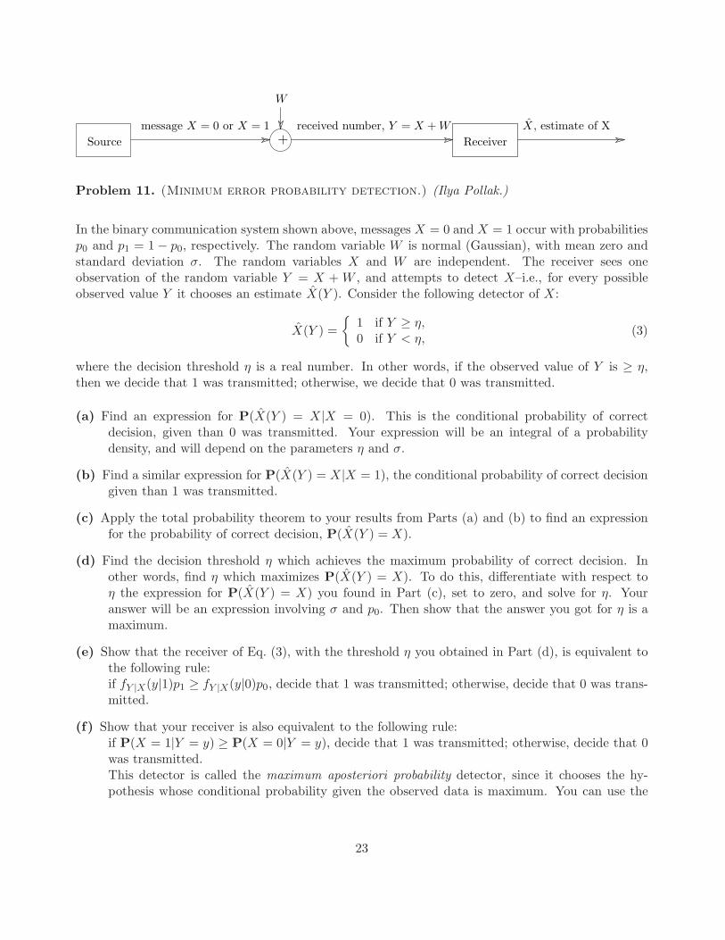
Problem 11. (Minimum error probability detection.) (Ilya Pollak.)
In the binary communication system shown above, messages X = 0 and X = 1 occur with probabilitiesp0 and p1 = 1 − p0, respectively. The random variable W is normal (Gaussian), with mean zero andstandard deviation σ. The random variables X and W are independent. The receiver sees oneobservation of the random variable Y = X + W , and attempts to detect X–i.e., for every possibleobserved value Y it chooses an estimate X(Y ). Consider the following detector of X:
X(Y ) =
{1 if Y ≥ η,0 if Y < η,
(3)
where the decision threshold η is a real number. In other words, if the observed value of Y is ≥ η,then we decide that 1 was transmitted; otherwise, we decide that 0 was transmitted.
(a) Find an expression for P(X(Y ) = X|X = 0). This is the conditional probability of correctdecision, given than 0 was transmitted. Your expression will be an integral of a probabilitydensity, and will depend on the parameters η and σ.
(b) Find a similar expression for P(X(Y ) = X|X = 1), the conditional probability of correct decisiongiven than 1 was transmitted.
(c) Apply the total probability theorem to your results from Parts (a) and (b) to find an expressionfor the probability of correct decision, P(X(Y ) = X).
(d) Find the decision threshold η which achieves the maximum probability of correct decision. Inother words, find η which maximizes P(X(Y ) = X). To do this, differentiate with respect toη the expression for P(X(Y ) = X) you found in Part (c), set to zero, and solve for η. Youranswer will be an expression involving σ and p0. Then show that the answer you got for η is amaximum.
(e) Show that the receiver of Eq. (3), with the threshold η you obtained in Part (d), is equivalent tothe following rule:if fY |X(y|1)p1 ≥ fY |X(y|0)p0, decide that 1 was transmitted; otherwise, decide that 0 was trans-mitted.
(f) Show that your receiver is also equivalent to the following rule:if P(X = 1|Y = y) ≥ P(X = 0|Y = y), decide that 1 was transmitted; otherwise, decide that 0was transmitted.This detector is called the maximum aposteriori probability detector, since it chooses the hy-pothesis whose conditional probability given the observed data is maximum. You can use the
23
following identities:
P(X = 1|Y = y) =fY |X(y|1)p1
fY (y),
P(X = 0|Y = y) =fY |X(y|0)p0
fY (y).
(g) Fix p0 = 0.5. What is the corresponding value of η? Sketch fY |X(y|1)p1 and fY |X(y|0)p0 for:
(i) σ = 0.1;
(ii) σ = 0.5;
(iii) σ = 1.
In each case, use the same coordinate axes for both functions. From looking at the plots, inwhich of the three cases would you expect the probability of correct decision to be the largest?the smallest? Use a table of the normal CDF to find the probability of correct decision in each ofthe three cases. What will happen to the probability of correct decision as σ → ∞? as σ → 0?
(h) Now suppose σ = 0.5 and p0 ≈ 1 (say, e.g., p0 = 0.9999). What is, approximately, the probabilityof correct decision? What is, approximately, the conditional probability P(X(Y ) = X|X = 1)?Suppose now that the message “X = 0” is “your house is not on fire” and the message “X = 1”,which has a very low probability, is “your house is on fire”. It may therefore be much morevaluable to correctly detect “X = 1” than “X = 0”. Suppose we get -$10 if we decide that thehouse is on fire when in fact it is, but that we get -$1000 if we decide that the house is not on firewhen in fact it is. Suppose further that we get $0 if we correctly decide that the house is not onfire, and that we get -$1 if we incorrectly decide that the house is on fire. It would make senseto maximize something other than the probability of correct decision. Propose such a criterion.(You do not have to find the optimal solution for the new criterion.)
Solution.
(a) When X = 0, Y = W . Hence we have:
fY |X(y|0) = fW (y) =1√2πσ
e−y2
2σ2 ,
P(X(Y ) = X|X = 0) = P(Y < η|X = 0) =
∫ η
−∞fY |X(y|0)dy =
∫ η
−∞
1√2πσ
e−y2
2σ2 dy.
(b) When X = 1, Y = 1 + W . Hence we have:
fY |X(y|1) = fW (y − 1) =1√2πσ
e−(y−1)2
2σ2 ,
P(X(Y ) = X|X = 1) = P(Y >= η|X = 1) =
∫ ∞
ηfY |X(y|1)dy =
∫ ∞
η
1√2πσ
e−(y−1)2
2σ2 dy.
24

(c) By the total probability theorem:
P(X(Y ) = X) = P(X(Y ) = X|X = 0)P(X = 0) + P(X(Y ) = X|X = 1)P(X = 1)
= p0
∫ η
−∞fY |X(y|0)dy + p1
∫ ∞
ηfY |X(y|1)dy. (4)
(d) For notational convenience, let us call φ(η) = P(X(Y ) = X). Taking the derivative of Eq. (4)with respect to η and equating it to zero, we get:
φ′(η) =dP(X(Y ) = X)
dη= p0fY |X(η|0) − p1fY |X(η|1) (5)
= p01√2πσ
exp
[
− η2
2σ2
]
− p11√2πσ
exp
[
−(η − 1)2
2σ2
]
= 0 (6)
⇒ p0
p1= exp
[η2 − (η − 1)2)
2σ2
]
= exp
[2η − 1
2σ2
]
⇒ ηmax = σ2 lnp0
p1+
1
2. (7)
Thus, ηmax is the unique extremum of φ(η). We now need to show that it’s a maximum. Notethat, if p0 > p1, then ηmax > 1/2. From the left side of Eq. (6), φ′(1/2) > 0–i.e., the function isincreasing on the left of ηmax, which means that ηmax is a maximum. Similarly, if p0 < p1, thenηmax < 1/2, and φ′(1/2) < 0, and so the function is decreasing on the right of ηmax, which meansthat ηmax is again a maximum. When p0 = 1/2, we infer from Eq. (4) that φ(∞) = φ(−∞) = 1/2whereas φ(ηmax) = φ(1/2) = Φ(1/(2σ)) > 1/2, which means that again, ηmax is a maximum.
(e) In Part (d), we showed that ηmax is the unique maximum of the function φ(η). This meansthat, for y < ηmax, φ′(y) > 0, and for y ≥ ηmax, φ′(y) ≤ 0. Using the expression for φ′(y) weobtained in Eq. (5), we see that this is equivalent to: if Y = y ≥ ηmax (i.e. we decide that 1was sent), then p0fY |X(y|0) ≤ p1fY |X(y|1); if Y = y < ηmax (we decide that 0 was sent), thenp0fY |X(y|0) > p1fY |X(y|1). This is illustrated in Fig. 7.
(f) Use
P(X = 1|Y = y) =fY |X(y|1)p1
fY (y),
P(X = 0|Y = y) =fY |X(y|0)p0
fY (y).
Combining these two equations with Part (e), we see that:
P(X = 1|Y = y) ≥ P(X = 0|Y = y) ⇔ p1fY |X(y|1) ≥ p0fY |X(y|0)⇔ decide that 1 was sent.
(g) Substituting p0 = 0.5 in Eq. (7), we immediately get:
ηmax = σ2 ln0.5
1 − 0.5+
1
2=
1
2.
25

2 1 0 1 2 30
0.1
0.2
0.3
0.4
0.5
0.6
0.7
y
Wei
ghte
d P
DF
of Y
con
ditio
ned
on X
eta
Figure 7: Weighted PDF’s of Y conditioned on X = 0 and on X = 1.
−2 −1 0 1 2 30
0.5
1
1.5
2
y
Wei
ghte
d P
DF
of Y
con
ditio
ned
on X
−2 −1 0 1 2 30
0.05
0.1
0.15
0.2
0.25
0.3
0.35
0.4
y
Wei
ghte
d P
DF
of Y
con
ditio
ned
on X
−2 −1 0 1 2 30
0.05
0.1
0.15
0.2
y
Wei
ghte
d P
DF
of Y
con
ditio
ned
on X
(a) σ = 0.1 (b) σ = 0.5 (c) σ = 1
Figure 8: Weighted PDF’s of Y conditioned on X.
(i,ii,iii) p1fY |X(y|1) and p0fY |X(y|0) for all the three cases are plotted in Fig. 8. Case (i) has thelargest probability of correct decision: among the three plots, this is the one where thesmallest portions of the conditional PDF’s “spill over” to the wrong side of the thresholdηmax = 1/2.
The probability of correct decision can be determined from Eq. (4):
P(X(Y ) = X) =1
2
∫ ηmax
−∞fY |X(y|0)dy +
1
2
∫ ∞
ηmax
fY |X(y|1)dy
=1
2Φ(ηmax
σ
)
+1
2
[
1 − Φ
(ηmax − 1
σ
)]
=1
2Φ
(1
2σ
)
+1
2
[
1 − Φ
(
− 1
2σ
)]
= Φ
(1
2σ
)
.
26

The probabilities of correct decision for the three cases are 0.9999997, 0.8413447, 0.6914624respectively.
When the noise is extremely large, it becomes impossible to distinguish between X = 0and X = 1; therefore, when σ → ∞, both the probability of correct decision and the errorprobability tend to 1/2. When σ → 0, the conditional PDF’s become very well concentratedaround their means; there is no noise in this case, and Y → X. The probability of correctdecision will tend to 1.
(h) When p0 is approximately 1, p1 is approximately 0. From Eq. (7), and also from Fig. 7, we cansee that ηmax goes to ∞ in this case. Therefore Eq. (4) becomes:
P(X(Y ) = X) ≈∫ ∞
−∞fY |X(y|0)dy = 1.
So we have probability 1 to make the correct decision: since it’s virtually certain that X = 0 istransmitted, the receiver just guesses X = 0 most of the time, and is correct most of the time.However, the conditional probability of correct decision given X = 1 is:
P(X(Y ) = X|X = 1} =
∫ ∞
ηmax
fY |X(y|1)dy
=
∫ ∞
∞fY |X(y|1)dy ≈ 0.
If we decide X = 0 all the time, we are bound to make an error whenever X = 1 is transmitted.Thus, even though the overall probability of error is miniscule, the conditional probability oferror given X = 1 is huge. Therefore, if it is very costly to us to make an error when X = 1(when, e.g., “X=1” is “your house is on fire”), it makes sense to try to minimize the expectedcost (rather than simply the probability of error)–i.e. the expected value of loss due to fire andfalse alarms:
minall estimators X(Y )
(10 · P(X = 1 and X = 1) + 1000 ·P(X = 0 and X = 1)
+ 1 ·P(X = 1 and X = 0)).
Problem 12. Gaussian mixture.A signal s = 3 is transmitted from a satellite but is corrupted by noise, and the received signal isX = s+W . When the weather is good, which happens with probability 2/3, W is a normal (Gaussian)random variable with zero mean and variance 4. When the weather is bad, W is normal with zeromean and variance 9. In the absence of any weather information:
(a) What is the PDF of X? (Hint. Use the total probability theorem.)
(b) Calculate the probability that X is between 2 and 4.
Solution.
27

(a) What we can do is to first find the CDF of X and then take its derivative to find the PDF. Bydefinition, we have:
FX(x) = P(X ≤ x).
Since we don’t have any weather information, if we can calculate the above probability condi-tioned on all the weather situations, we can apply the total probability theorem to get the finalanswer. If the weather is good, the random variable X = 3 + W is conditionally normal withmean µ = 3 and variance σ2 = 4. In this case, the conditional probability that X is less than orequal to some x is:
P (X ≤ x|good) = Φ
(x − µ
σ
)
= Φ
(x − 3
2
)
Similarly, if we suppose the weather is bad, the conditional probability is:
P (X ≤ x|bad) = Φ
(x − µ
σ
)
= Φ
(x − 3
3
)
Apply the total probability theorem to get:
FX(x) = P (X ≤ x) = P (X ≤ x|good)P (good) + P (X ≤ x|bad)P (bad)
= Φ
(x − 3
2
)2
3+ Φ
(x − 3
3
)1
3
Finally,
fX(x) =dFX(x)
dx=
2
3
1√2π2
e−(x−3)2
2·22 +1
3
1√2π3
e−(x−3)2
2·32
=1
3
1√2π
e−(x−3)2
8 +1
9
1√2π
e−(x−3)2
18
In general, the total probability theorem implies that, if B1, B2, · · · , Bn partition the samplespace, the following is true for any continuous random variable X:
fX(x) = fX|B1(x)P (B1) + fX|B2
(x)P (B2) + · · · + fX|Bn(x)P (Bn).
(b) To calculate P (2 ≤ X ≤ 4), we use our results from Part (a):
P (2 ≤ X ≤ 4) = P (X ≤ 4) − P (X ≤ 2) = FX(4) − FX(2)
= Φ
(4 − 3
2
)2
3+ Φ
(4 − 3
3
)1
3−[
Φ
(2 − 3
2
)2
3+ Φ
(2 − 3
3
)1
3
]
= Φ
(1
2
)2
3+ Φ
(1
3
)1
3−[
Φ
(−1
2
)2
3+ Φ
(−1
3
)1
3
]
≈ 2
3· 2 · 0.19146 +
1
3· 2 · 0.12930 = 0.3415.
Problem 13. (Ilya Pollak.)Consider the following joint PDF of two continuous random variables, X and Y:
fXY (x, y) =
{A, 0 ≤ x ≤ 2 and 0 ≤ y ≤ 20, otherwise.
28

(a) Find A.
(b) Find the marginal PDFs fX(x) and fY (y).
(c) Are X and Y uncorrelated? Are they independent?
(d) Find E[Y ] and V ar(Y ).
(e) Let Z = X + Y . Find the conditional PDF fZ|X(z|x), as well as the marginal PDF fZ(z) of Z.
Solution. Note that fXY (x, y) can be written as A(u(x)− u(x− 2))(u(y)− u(y − 2)) for all x, y ∈ R.
(a) The integral of fXY (x, y) over the whole real plane must be 1:
∫
R2
fXY (x, y)dxdy =
∫
R2
A(u(x) − u(x − 2))(u(y) − u(y − 2))dxdy
= A
∫ 2
0
∫ 2
01dxdy
= A · 4 = 1.
Therefore we get A = 1/4.
(b) To get the marginal density of X, integrate the joint density:
fX(x) =
∫ ∞
−∞fXY (x, y)dy
=
∫ ∞
−∞0.25(u(x) − u(x − 2))(u(y) − u(y − 2))dy
= 0.25(u(x) − u(x − 2))
∫ ∞
−∞(u(y) − u(y − 2))dy
= 0.25(u(x) − u(x − 2))
∫ 2
01 dy
= 0.5(u(x) − u(x − 2)).
So X is uniformly distributed on [0,2].
fY (y) =
∫ ∞
−∞fXY (x, y)dx
= 0.25(u(y) − u(y − 2))
∫ ∞
−∞(u(x) − u(x − 2))dx
= 0.5(u(y) − u(y − 2)).
Y is also uniformly distributed on [0,2].
(c) From Parts (a) and (b), we have fXY (x, y) = fX(x)fY (y). By definition of independence, X andY are independent, and therefore also uncorrelated.
29

(d) By definition of expectation and variance,
E[Y ] =
∫ ∞
−∞yfY (y)dy
=
∫ 2
00.5ydy = 1.
V ar(Y ) = E[(Y − E[Y ])2] = E[Y 2] − (E[Y ])2
=
∫ 2
00.5y2dy − 1
= 0.5(1/3)y3∣∣2
0− 1
= 4/3 − 1 = 1/3.
(e) When X = x, Z = x + Y . Therefore,
FZ|X(z|x) = P(Z ≤ z|X = x)
= P(Y ≤ z − x|X = x)
= P(Y ≤ z − x) (because X and Y are independent)
= FY (z − x).
Differentiating with respect to z, we get:
fZ|X(z|x) =∂FZ|X(z|x)
∂z= fY (z − x) = 0.5(u(z − x) − u(z − x − 2)).
The PDF of Z can be obtained as follows:
fZ(z) =
∫ ∞
−∞fXZ(x, z)dx =
∫ ∞
−∞fZ|X(z|x)fX(x)dx
=
∫ ∞
−∞fY (z − x)fX(x)dx = fY ∗ fX(z)
=
∫ ∞
−∞0.5(u(z − x) − u(z − x − 2))0.5(u(x) − u(x − 2))dx
=
∫ 2
00.25(u(z − x) − u(z − x − 2))dx
=
z/4, 0 ≤ z ≤ 21 − z/4, 2 < z ≤ 4
0, otherwise
Problem 14. Scalar vs vector quantization. (Ilya Pollak.)
Many physical quantities can assume an infinite number of values. In order to store them digitally,they need to be approximated using a finite number of values. If the approximated quantity can
30

have r possible values, it can be stored using ⌈log2 r⌉ bits, where ⌈x⌉ denotes the smallest integer notexceeding x.
For example, in the physical world, an infinite number of shades of different colors is possible; howevercapturing a picture with a digital camera and storing it requires (among other things!) approximatingthe color intensities using a finite range of values, for example, 256 distinct values per color channel.Audio signals can similarly have an infinite range of values; however, in order to record music to aniPod or a CD, a similar approximation is required.
In addition, most of real-world data storage and transmission applications involve lossy data compression—i.e., the use of algorithms that can encode data at different quality levels, through a trade-off betweenquality and file size. Widely used examples of such algorithms are JPEG (for still pictures), H.264(for video), and MP3 (for audio). All such lossy data compression schemes involve approximatingvariables that can assume 2k values with variables that can only assume 2n values, with n < k.
This process of approximating a variable X that can assume more than 2n different values, withanother variable Y that can only assume 2n different values, is called n-bit quantization.
Suppose A1 and A2 are two random variables with the following joint PDF:
fA1,A2(a1, a2) =
12 , if both 0 ≤ a1 ≤ 1 and 0 ≤ a2 ≤ 1;12 , if both 1 ≤ a1 ≤ 2 and 1 ≤ a2 ≤ 2;0, otherwise.
(a) Find the marginal PDF of A1, fA1(a1).
(b) One-bit Lloyd-Max quantizer. Suppose we want to quantize A1 to one bit, in the followingway. We pick three real numbers x0, q1, and q2. If A1 < x0 we quantize it to q1. If A1 ≥ x0 wequantize it to q2. In other words, the quantized version A1 of A1 is determined as follows:
A1 =
{q1, if A1 < x0
q2, if A1 ≥ x0
Note that, since A1 can only assume one of two values, any observation of A1 can be stored usingone bit. Unfortunately, A1 will be only an approximation of A1. Find the numbers x0, q1, andq2 which minimize the mean-square error (MSE),
E[(A1 − A1)2]. (8)
It can be shown that 0 ≤ q1 ≤ x0 ≤ q2 ≤ 2. You can just assume that these inequalities hold,without proof.
(c) Calculate the mean-square error defined in Eq. (8) for the quantizer that you obtained in Part(b).
(d) Show that the marginal PDF of A2 is the same as the marginal PDF of A1. Therefore, theone-bit Lloyd-Max quantizer for A2 is identical to the one for A1 which you obtained in Part(b), and
E[(A2 − A2)2] = E[(A1 − A1)
2]. (9)
31

(e) Suppose now we need to quantize both A1 and A2, and our bit budget is 2 bits. One way ofdoing this would be to use a one-bit Lloyd-Max quantizer derived in Part (b) for A1, and usethe same quantizer for A2:
A2 =
{q1, if A2 < x0
q2, if A2 ≥ x0,
where x0, q1, and q2 are the numbers found in Part (b).
Consider an alternative procedure for quantizing the same variables, using the same number ofbits:
A′1 = A′
2 =
1/3, if A1 + A2 < 12/3, if 1 ≤ A1 + A2 < 24/3, if 2 ≤ A1 + A2 < 35/3, if A1 + A2 ≥ 3
(10)
Such a quantization strategy where two or more variables are quantized jointly is called vectorquantization, as opposed to scalar quantization which quantizes one variable at a time. Theparticular quantizer of Eq. (10) can be viewed as using both bits to quantize A1 (since there arefour quantization levels for A1), and using zero bits to quantize A2: once A′
1 is stored, A′2 does
not need to be stored at all, since it is equal to A′1.
For this new quantizer, find the mean-square errors,
E[(A′1 − A1)
2] and E[(A′2 − A2)
2]. (11)
Compare your results with Eq. (8) and (9), and explain why this new quantizer is able to achievesmaller errors with the same number of bits.
(Hint. For this problem, it may be very helpful to draw, in the a1-a2 plane, the set of all points wherethe joint PDF of A1 and A2 is non-zero. In the same picture, draw all possible points (A1, A2). Thendraw all possible points (A′
1, A′2).)
Solution. The joint PDF of A1 and A2 is illustrated in Fig. 9(a). It shows that the the random vector(A1, A2) can only appear in the shaded region, with uniform probability.
(a)
fA1(a1) =
∫ ∞
−∞fA1,A2(a1, a2)da2
=
0 a1 < 0 or a1 > 2∫ 1
0
12da2 = 1
2 0 ≤ a1 ≤ 1∫ 2
1
12da2 = 1
2 1 ≤ a1 ≤ 2
=1
2[u(a1) − u(a1 − 2)].
This is a uniform distribution over [0, 2].
32

1
1
2
21a
2a
1/2
1/2
1
1
2
21a
2a
I
II
III
IV
),( 21 qq
),( 12 qq
),( 22 qq
),( 11 qq
1
1
2
21a
2a
I
II
)3/1,3/1(
)3/5,3/5(
)3/4,3/4(
)3/2,3/2(I
II
III
IV
(a) Joint PDF of A1 and A2. (b) Quantizer in Parts (b-d). (c) Quantizer in Part (e).
Figure 9: Problem 14.
(b) Since the marginal PDF of A1 is uniform between 0 and 2, having x0 ≤ 0 would waste half ofour bit on values that have probability zero. Having x0 ≥ 2 would be similarly wasteful. Hence0 < x0 < 2. If q1 < 0, the mean-square error can always be reduced by setting q1 = 0. Ifq1 > x0, the mean-square error can be reduced by setting q1 = x0. Hence, 0 ≤ q1 ≤ x0. Asimilar argument shows that x0 ≤ q2 ≤ 2. Therefore, the mean-square error can be rewritten as:
E[(A1 − A1)2] =
∫ ∞
−∞(a1 − a1)
2fA1(a1)da1
=
∫ x0
0(q1 − a1)
2fA1(a1)da1 +
∫ 2
x0
(q2 − a1)2fA1(a1)da1
=1
2
∫ x0
0(q1 − a1)
2da1 +1
2
∫ 2
x0
(q2 − a1)2da1. (12)
In order to minimize Eq. (12) over all possible x0, q1, and q2, we take the partial derivative of(12) with respect to each of these variables and equate it to zero:
∂E[(A1 − A1)2]
∂x0=
1
2(q1 − x0)
2 − 1
2(q2 − x0)
2 = 0,
∂E[(A1 − A1)2]
∂q1=
1
2
∫ x0
02(q1 − a1)da1 = 0,
∂E[(A1 − A1)2]
∂q2=
1
2
∫ 2
x0
2(q2 − a1)da1 = 0.
After some simplifications, we get:
x0 = (q1 + q2)/2, (13)
q1 = x0/2, (14)
q2 = (x0 + 2)/2. (15)
33

The solution to Eqs. (13)-(15) is:
x0 = 1, q1 = 0.5, q2 = 1.5.
Evaluating the second derivatives of the MSE at this solution,
∂2E[(A1 − A1)2]
∂x20
= (x0 − q1) − (x0 − q2) = q2 − q1 = 1 > 0,
∂2E[(A1 − A1)2]
∂q21
=
∫ x0
0da1 = x0 = 1 > 0,
∂2E[(A1 − A1)2]
∂q22
=
∫ 2
x0
da1 = 2 − x0 = 1 > 0,
we see that the extremum we found is a minimum.
(c) With the values we obtained in Part (b), the mean-square error of the quantizer is:
E[(A1 − A1)2] =
1
2
∫ 1
0
(1
2− a1
)2
da1 +1
2
∫ 2
1
(3
2− a1
)2
da1
=1
12.
(d) If a1 and a2 are interchanged, the joint PDF of A1 and A2 will remain the same. This symmetrymeans that the marginal PDF of A2 is the same as the marginal PDF of A1, and that theprocedure to obtain the optimal quantizer for A2 is also identical to part (b). Therefore, A2
must have the same minimum MSE quantizer as A1, with the same value for MSE.
(e) The new quantizer is illustrated in Fig. 9(c). The outcomes of the random vector in triangle Iget quantized to (1/3, 1/3), outcomes in triangle II get quantized to (2/3, 2/3), etc. The MSE ofquantizing A1 can be broken into four integrals over the four triangles. Since the triangles arecongruent, and since the positions of quantization points within the triangles are identical, thefour integrals will be the same. Therefore, to get the MSE, we need to evaluate just one of theintegrals and multiply the result by 4:
E[(A′1 − A1)
2] = 4
∫
I
(1
3− a1
)2
fA1,A2(a1, a2)da1da2
= 4
∫ 1
0
∫ 1−a1
0
(1
3− a1
)2 1
2da2da1
= 2
∫ 1
0
(1
3− a1
)2
(1 − a1)da1
= 2
∫ 1
0
(1
3− a1
)3
da1 + 2
∫ 1
0
(1
3− a1
)2 2
3da1
= −2
∫ 1
0
(
a1 −1
3
)3
da1 +4
3
∫ 1
0
(
a1 −1
3
)2
da1
34

= −2
(a1 − 1
3
)4
4
∣∣∣∣∣
1
0
+4
3
(a1 − 1
3
)3
3
∣∣∣∣∣
1
0
= −1
2
(2
3
)4
+1
2
(
−1
3
)4
+4
9
(2
3
)3
− 4
9
(
−1
3
)3
= − 16
2 · 81 +1
2 · 81 +32
3 · 81 +4
3 · 81 = − 15
2 · 81 +36
3 · 81 =24 − 15
2 · 81=
1
18.
By symmetry, E[(A′2 − A2)
2] = E[(A′1 − A1)
2] = 118 .
The quantizer of Parts (b)-(d) was designed separately for A1 and A2, based on the knowledge ofthe marginal PDF’s of A1 and A2, but without exploiting the fact that A1 and A2 are dependent.This way, out of the four quantization points, (1/2, 1/2), (1/2, 3/2), (3/2, 1/2), and (3/2, 3/2),only two–(1/2, 1/2) and (3/2, 3/2)–have a nonzero probability (see Fig. 9(b)). The other twopoints are wasted on coding impossible events. Therefore, our algorithm does not take fulladvantage of the two bits. The quantizer in Part (e) exploits dependence of A1 and A2, bytrying to distribute the four quantization points evenly (more or less) throughout the regionwhere the joint PDF of A1 and A2 is non-zero. Through this better placement of quantizationpoints, it is able to achieve a smaller MSE.
Problem 15. (Montier, [4].)You will represent Company A (the potential acquirer), which is currently considering acquiring Com-pany T (the target) by means of a tender offer. The main complication is this: the value of Company Tdepends directly on the outcome of a major oil exploration project that is currently being undertaken.If the project fails, the company under current management will be worth nothing ($0). But if theproject succeeds, the value of the company under current management could be as high as $100 pershare. All share values between $0 and $100 are considered equally likely.
By all estimates, Company T will be worth considerably more in the hands of Company A than undercurrent management. In fact, the company will be worth 50% more under the management of A thanunder the management of Company T. If the project fails, the company will be worth zero undereither management. If the exploration generates a $50 per share value, the value under Company Awill be $75. Similarly, a $100 per share under Company T implies a $150 value under Company A,and so on.
It should be noted that the only possible option to be considered is paying in cash for acquiring 100%of Company T’s shares. This means that if you acquire Company T, its current management will nolonger have any shares in the company, and therefore will not benefit in any way from the increase inits value under your management.
The board of directors of Company A has asked you to determine whether or not to submit an offerfor acquiring company T’s shares, and if so, what price they should offer for these shares. This offermust be made now, before the outcome of the drilling project is known. Company T will accept anyoffer from Company A, provided it is at a profitable price for them. It is also clear that CompanyT will delay its decision to accept or reject your bid until the results of the drilling project are in.Thus you (Company A) will not know the results of the exploration project when submitting your
35

price offer, but Company T will know the results when deciding on your offer. As already explained,Company T is expected to accept any offer by Company A that is greater than the (per share) valueof the company under current management, and to reject any offers that are below or equal to thisvalue. Thus, if you offer $60 per share, for example, Company T will accept if the value under currentmanagement is anything less than $60. You are now requested to give advice to the representative ofCompany A who is deliberating over whether or not to submit an offer for acquiring Company T’sshares, and if so, what price he/she should offer for these shares. If your advice is that he/she shouldnot acquire Company T’s shares, advise him/her to offer $0 per share. If you think he/she should tryto acquire Company T’s shares, advise him/her to offer anything above $0 per share. What is theoffer that he/she should make? In other words, what is the optimal offer?
Solution. (Ilya Pollak.)Let X be the share price after the drilling project results are known. Let y be our offer, in dollars.Note that 0 ≤ y ≤ 100. This is because making an offer above $100 does not make sense: CompanyT is never worth more than $100 per share under the current management, and so an offer of $100 orabove is sure to be accepted. To compute Company A’s expected profit per share, we consider twocases separately:
• Case 1: y > X. The offer is accepted, and Company A makes 1.5X − y.
• Case 2: y ≤ X. The offer is rejected, and Company A makes 0.
Based on the problem statement, to us X is a random variable. Using the total expectation theoremand the linearity of expectation, we have that the expected profit for Company A is:
E[1.5X − y|y > X] ·P(y > X) + E[0|y ≤ X] · P(y ≤ X) = (1.5E[X|X < y] − E[y|X < y])P(X < y)
= (1.5E[X|X < y] − y)P(X < y)
To evaluate this expression, we need to interpret the statement from the problem formulation thatsays: “All share values between $0 and $100 are considered equally likely.” This implies a uniformdistribution for the random variable X; however, there are several different reasonable assumptionsthat we can make. The random variable X can be modeled as either a continuous or a discrete uniformrandom variable. In the case of a discrete uniform distribution, we need to make further modelingassumptions regarding the granularity.
First, assuming that X is a continuous uniform random variable, we get that the conditional PDF ofX given that X < y is uniform between 0 and y, and therefore the conditional expectation of X giventhat X < y is y/2. Hence, the expected profit is:
(1.5(y/2) − y)P(X < y) = −0.25yP(X < y).
Therefore, the largest possible profit is zero, and is achieved when y = 0. The optimal strategy is notto make an offer.
Alternatively, we can assume that prices change in increments of one cent, and therefore X is a discreteuniform random variable, with possible values being all integer multiples of $0.01, from zero to $100.In this case, the conditional PMF of X given that X < y, for any y > 0, is uniform between 0 and
36

y − 0.01, and therefore the conditional expectation of X given that X < y is y/2 − 0.005. Hence, forany positive offer price y, the expected profit is:
(1.5(y/2 − 0.005) − y)P(X < y) = −(0.25y + 0.0075)P(X < y).
This is still negative, hence still the best strategy is not to make an offer.
Another reasonable alternative is to assume that prices change in increments of one dollar. In thiscase, X is a discrete uniform random variable, with possible values being all integers between 0 and$100. The conditional PMF of X given X < y, for any y > 0, is uniform between 0 and y − 1, andtherefore the conditional expectation of X given that X < y is y/2− 0.5. Hence, for any positive offerprice y, the expected profit is:
(1.5(y/2 − 0.5) − y)P(X < y) = −(0.25y + 0.75)P(X < y).
This is again negative, hence still the best strategy is not to make an offer.
Problem 16. Optimal portfolios. (Ilya Pollak.)This problem illustrates why it is good to diversify your investments. If you are able to split yourinvestment among several independent assets, you will have a lower risk than if you invest everythingin a single asset.
(a) You have $1 to invest in two assets. Denote the yearly return from Asset 1 by R1 and the yearlyreturn from Asset 2 by R2. This means that every dollar invested in Asset 1 will turn into$(1 + R1) by the end of one year, and every dollar invested in Asset 2 will turn into $(1 + R2).Suppose that R1 and R2 are independent continuous random variables with
E[R1] = E[R2] = 0.1
var(R1) = 0.04
var(R2) = 0.09
How should you allocate your $1 between the two assets in order to minimize risk, as measuredby the standard deviation of your return?
Find the expected value and the standard deviation of the resulting return, and compare to themeans and standard deviations for investing the entire $1 into Asset 1 and into Asset 2.
Hint. Denote the amounts invested in Assets 1 and 2 by a and 1 − a, respectively (0 ≤ a ≤ 1).Then the return of your portfolio is R = aR1 + (1 − a)R2. Find the value of a which minimizesthe standard deviation of the portfolio return R. Note that minimizing the standard deviationis equivalent to minimizing the variance, but the expression for the variance is more convenientto differentiate. Then, for the value of a that you obtain, find E[R] and var(R).
Solution. Using the independence of R1 and R2, we have:
var(R) = var(aR1 + (1 − a)R2)
= var(aR1) + var((1 − a)R2)
= a2var(R1) + (1 − a)2var(R2)
= 0.04a2 + 0.09 − 0.18a + 0.09a2
= 0.13a2 − 0.18a + 0.09.
37

This is a parabola and hence has a unique extremum. Since the coefficient of a2 is positive, theextremum is a minimum. To find its location, take the derivative and set to zero:
0.26a − 0.18 = 0
a =9
13≈ 0.69
Thus we are investing $ 913 into Asset 1, and $ 4
13 into Asset 2, for a total return of
R =9
13R1 +
4
13R2
Since expectations are linear, we have:
E[R] =9
13E[R1] +
4
13[R2] = 0.1
Since the mean returns of Asset 1 and Asset 2 are 10% each, the mean portfolio return willalways be 10%, regardless of how the two assets are weighted in the portfolio.
To find the variance, we substitute a = 9/13 into the formula derived above:
var(R) = a2var(R1) + (1 − a)2var(R2)
=
(9
13
)2
· 0.04 +
(4
13
)2
· 0.09
=3.24 + 1.44
169
=468
16900
=117
4225≈ 0.0277
Therefore, the standard deviation of the portfolio return is
σR =
√
117
4225≈ 0.166
Note that the standard deviations of Assets 1 and 2 are 0.2 and 0.3, respectively. Our portfoliohas standard deviation of 0.166, which is lower than both the standard deviation of Asset 1 andthe standard deviation of Asset 2. By mixing together two risky but independent assets, wehave obtained a portfolio which is less risky than either one of the two assets, but has the sameexpected return.
(b) Assume the same means and variances for R1 and R2 as in Part (a), but now assume that R1
and R2 are correlated, with covariance
cov(R1, R2) = 0.03,
and correlation coefficient
ρR1,R2 =cov(R1, R2)
σR1σR2
=0.03
0.2 · 0.3 = 0.5.
38

Repeat Part (a) for these new conditions, i.e., find the portfolio weights a and 1−a that minimizethe variance of the portfolio return, and find the resulting variance and standard deviation ofthe portfolio return.
Solution. Since R = aR1 + (1 − a)R2, we have:
var(R) = var(aR1 + (1 − a)R2)
= a2var(R1) + (1 − a)2var(R2) + 2a(1 − a)cov(R1, R2) (16)
Therefore,
d
davar(R) = 2avar(R1) − 2(1 − a)var(R2) + (2 − 4a)cov(R1, R2)
= 2[a(var(R1) + var(R2) − 2cov(R1, R2)) − var(R2) + cov(R1, R2)]
Setting the derivative to zero yields:
a(var(R1) + var(R2) − 2cov(R1, R2)) = var(R2) − cov(R1, R2)
a =var(R2) − cov(R1, R2)
var(R1) + var(R2) − 2cov(R1, R2)
=0.09 − 0.03
0.04 + 0.09 − 2 · 0.03=
0.06
0.07=
6
7
The second derivative is:
d2
da2var(R) = 2(var(R1) + var(R2) − 2cov(R1, R2))
= 2(0.04 + 0.09 − 2 · 0.03) = 0.14 > 0,
and therefore the extremum we found is a minimum. Substituting a = 6/7 into Eq. (16), we get:
var(R) =
(6
7
)2
· 0.04 +
(1
7
)2
· 0.09 + 2 · 6
7· 1
7· 0.03
= 0.01 · 144 + 9 + 36
49=
189
4900≈ 0.0386.
Therefore, the standard deviation of the portfolio return is now
σR =
√
189
4900≈ 0.196.
This is still a little smaller than the standard deviation 0.2 of Asset 1; however, since Asset 2 isnow significantly correlated with Asset 1 (correlation coefficient 0.5), it does not provide muchdiversification to our portfolio.
(c) Suppose three assets have returns R1, R2, and R3 which are independent random variableswith means E[R1] = 0.05, E[R2] = 0.1, and E[R3] = 0.15, and variances var(R1) = 0.01,
39

var(R2) = 0.04, and var(R3) = 0.09. Suppose you want to invest $1 into these three assetsso that your expected return is 0.1, and your risk is as small as possible. In other words, youinvest a1 in Asset 1, 1 − a1 − a3 in Asset 2, and a3 in Asset 3, and obtain a portfolio whosereturn is R = a1R1 + (1− a1 − a3)R2 + a3R3. Find a1 and a3 to minimize var(R) subject to theconstraint E[R] = 0.1. For these values of a1 and a3, find the variance and standard deviationof the portfolio return R.
Solution. The expected portfolio return is:
E[R] = a1E[R1] + (1 − a1 − a3)E[R2] + a3E[R3]
= 0.05a1 + 0.1(1 − a1 − a3) + 0.15a3
= 0.1 − 0.05a1 + 0.05a3.
In order for the expected portfolio return to be equal to 0.1, we must therefore have a1 = a3. Ifthis is the case, we have that the variance of the portfolio return is:
var(R) = a21var(R1) + (1 − 2a2)
2var(R2) + a21var(R3)
= a21[var(R1) + 4var(R2) + var(R3)] − 4a1var(R2) + var(R2)
= a21[0.01 + 0.16 + 0.09] − 0.16a1 + 0.04
= 0.26a21 − 0.16a1 + 0.04.
Differentiating and setting the derivative to zero yields 0.52a1 − 0.16 = 0, and therefore thesolution is a1 = 0.16/0.52 = 4/13. Since the second derivative is positive, this is a minimum.The weights for Assets 3 and 2 are a3 = a1 = 4/13 and a2 = 1 − a1 − a3 = 5/13. For theseweights, the variance of the portfolio return is:
var(R) = 0.26
(4
13
)2
− 0.16 · 4
13+ 0.04
= 0.02 · 16
13− 0.64
13+
0.52
13
=0.2
13=
1
65≈ 0.0154.
The standard deviation is
σR =
√
1
65≈ 0.124.
(d) Suppose you are now allocating your $1 among ten assets with independent returns. The ex-pected return for each asset is 0.1. The return variances are 1, 1/2, 1/3, . . . , 1/10. Find theallocation weights a1, a2, . . ., a9, 1 − a1 − a2 − . . . − a9 that minimize the variance of yourportfolio return. Find the variance and standard deviation of the portfolio return for theseweights.
Solution. Since the returns of individual assets are independent, we have:
var(R) =10∑
i=1
a2i var(Ri)
=
9∑
i=1
a2i var(Ri) +
(
1 −9∑
i=1
ai
)2
var(R10),
40

where we used the notation
a10 = 1 −9∑
i=1
ai.
To get the minimum of the variance, we set to zero its partial derivatives with respect to a1, . . . , a9
and then check that the second partial derivatives are positive. The first partial derivative withrespect to ai is:
∂
∂aivar(R) = 2aivar(Ri) + 2
(
1 −9∑
i=1
ai
)
(−1)var(R10)
= 2aivar(Ri) − 2a10var(R10).
For this to be zero for all i = 1, . . . , 9, we therefore must have:
ai = a10var(R10)
var(Ri), (17)
for i = 1, . . . , 9. Note that this identity also holds for i = 10. Since the sum of the ten weightsmust be equal to one, we obtain the following by summing the above equation over i = 1, . . . , 10:
1 = a10var(R10)10∑
i=1
1
var(Ri),
and hence
a10 =1
var(R10)∑10
i=11
var(Ri)
.
Substituting this into Eq. (17), we get:
ai =1
var(Ri)∑10
j=11
var(Rj)
=1
1i
∑10j=1 j
=i
55.
The second partial derivative of the variance is
∂2
∂a2i
var(R) = 2var(Ri) + 2var(R10) > 0,
which means that we found a minimum. Substituting the values of the weights we found into the
41
expression for the variance, we get the following value of the variance for our optimal portfolio:
var(R) =10∑
i=1
(i
55
)2
var(Ri)
=10∑
i=1
(i
55
)2 1
i
=
10∑
i=1
i
552
=1
55,
which is significantly lower than the variance of any single asset in the portfolio. The standarddeviation is:
σR =
√
1
55≈ 0.135.
Problem 17. Simulating a fair coin with a biased one. (After Bertsekas-Tsitsiklis [1] andStout-Warren [5].)
An NFL referee has only one biased coin available for the pre-game coin toss. For this coin, theprobability of heads is 0.6, and both the referee and the two teams know this. The referee would liketo devise a coin-tossing procedure that each team will have a 0.5 probability of winning. Problem 1.33in the recommended text [1] suggests the following strategy: Have one team call HT or TH and flipthe coin twice. If the result is HH or TT, the procedure is repeated.
(a) What is the probability to have to keep going after the n-th independent repetition of thisprocedure? In other words, what is the probability that no single trial among the n independenttrials results in HT or TH?
Solution. If a biased coin with probability of heads p is independently tossed twice, the proba-bility of HH is p2 and the probability of TT is (1 − p)2. The probability to keep getting HH orTT in n independent repetitions of this procedure is therefore (p2 + (1− p)2)n. In our case, thisis (0.62 + 0.42)n = 0.52n.
(b) What is the probability to never terminate, i.e., to keep getting HH or TT forever?
Solution. The probability to keep getting HH or TT forever is limn→∞(p2 + (1 − p)2)n whichis zero, as long as 0 < p < 1.
(c) What is the expected number of repetitions of this procedure required to terminate, i.e., to getan outcome that’s either HT or TH? What is the expected number of coin flips required toterminate this procedure?
Solution. The number of repetitions to achieve an HT or TH is a geometric random variablewith probability of success 2p(1 − p) = 0.48 which means that its expectation is 1/0.48 ≈ 2.08.
42

Since each repetition of the procedure consists of two coin flips, the expected number of coinflips is 2 · 2.08 = 4.16.
(d) There exist many other more complicated algorithms that are more efficient—i.e., achieve asmaller expected value. These algorithms exploit the fact that there exist other equiprobablesequences, for example, HHTT and TTHH. (See, e.g., [5].) For instance, the first team couldbet on HT, HHHT, TTHT or HHTT, and the second on TH, HHTH, TTTH or TTHH. Ifnone of these come up, the procedure is repeated. This is still fair: each team has probabilityp(1− p) + p2(1− p)2 + p3(1− p) + p(1− p)3 of winning in one round of the procedure. Calculatethe expected number of flips for this strategy. One way of doing this it to follow these steps:
(i) Find the probabilities R2 and R4 to terminate after two and four flips, respectively.
Solution.
R2 = 2p(1 − p) = 0.48
R4 = 2(p2(1 − p)2 + p3(1 − p) + p(1 − p)3) = 2(0.0576 + 0.0864 + 0.0384) = 0.3648
(ii) Let RT = R2 +R4 be the probability to terminate in one round. Let N be the total numberof rounds required to terminate (i.e., to determine the winner.) Express E[N ] as a functionof RT .
Solution. The total number of required rounds is geometric with parameter RT , andtherefore the expected total number of rounds is 1/RT .
(iii) Given that N = n, find the conditional probabilities that the N -th round consists of twoflips and that the N -th round consists of four flips.
Solution. Given that we have to go exactly N rounds, the conditional probability that theN -th round consists of two flips is R2/(R2 + R4) ≈ 0.568, and the conditional probabilitythat the N -th round consists of four flips is R4/(R2 + R4) ≈ 0.432.
(iv) If the total number of rounds is N = n, then the total number of flips is 4(n − 1) plus thenumber of flips in the last round. Use this observation in conjunction with the result ofpart (iii) to find the conditional expectation of the total number of flips Nf given that thetotal number of rounds is N = n.
Solution. Using the total expectation theorem, the conditional expectation of the numberof flips given N = n rounds is:
E[Nf |N = n] =R2
R2 + R4(4n − 2) +
R4
R2 + R4(4n) =
4n(R2 + R4) − 2R2
R2 + R4≈ 4n − 1.136.
(v) Use the iterated expectation formula to find the expected number of flips E[Nf ].
Solution. Using the iterated expectation formula, the expected number of flips is:
E[E[Nf |N ]] =4E[N ](R2 + R4) − 2R2
R2 + R4
=4 − 2R2
R2 + R4
=4 − 2 · 0.48
0.8448=
3.04
0.8448≈ 3.60,
which is about 13% faster than the 4.16 flips expected under the simpler strategy.
43

Problem 18. (Ilya Pollak.)The CDF of a continuous random variable X is:
FX(x) =
0, x < 0x/2, 0 ≤ x ≤ 21, x > 2
a. Find the PDF of X.
Solution. Differentiating the CDF, we get:
fX(x) =
0, x < 01/2, 0 < x < 20, x > 2
Thus, X is a continuous random variable, uniformly distributed between 0 and 2. Note that thederivative of the CDF does not exist at x = 0 and at x = 2.
b. Find E[X].
Solution. E[X] = (0 + 2)/2 = 1.
c. Find var(X).
Solution. var(X) = (2 − 0)2/12 = 1/3.
d. Find E[X3].
Solution.
E[X3] =
∫ 2
0x3/2 dx =
x4
8
∣∣∣∣
2
0
= 16/8 = 2.
e. Find the conditional PDF of X given that 0 < X < 1/2.
Solution. Given that 0 < X < 1/2, the conditional PDF of X is zero outside of the region0 < x < 1/2. Inside the region, it is equal to the PDF of X divided by the probability of 0 < X <
1/2. For 0 < x < 1/2, the PDF is 1/2 as found in Part a. P(0 < X < 1/2) =∫ 1/20 1/2 dx = 1/4.
Hence, we get:
fX|0<X<1/2(x) =
0, x < 02, 0 < x < 1/20, x > 1/2
An alternative way of arriving at the same answer is simply to notice that, since the PDF of Xis uniform over 0 ≤ x ≤ 2, the conditional PDF of X given 0 < X < 1/2 must be uniform over0 < x < 1/2.
f. Find the PDF of the random variable Y = X − 1.
Solution. First, find the CDF:
FY (y) = P(Y ≤ y) = P(X − 1 ≤ y) = P(X ≤ y + 1) = FX(y + 1)
44

Then differentiate to find the PDF:
fY (y) =d
dyFX(y + 1) = fX(y + 1) =
0, y < −11/2, −1 < y < 10, y > 1
As a quick check, note that, since X is between 0 and 2 with probability 1, Y = X − 1 must bebetween −1 and 1 with probability 1.
An alternative method is to note that by subtracting 1 from a random variable, we move itsPDF to the left by 1. Hence, the PDF of Y is uniform from −1 to 1.
Problem 19. (Ilya Pollak.)Consider the following joint PDF of two continuous random variables, X and Y :
fXY (x, y) =
{1, 0 ≤ x ≤ 1 and 0 ≤ y ≤ 10, otherwise.
a. Find the marginal PDF fX(x).
Solution. To get the marginal density of X, integrate the joint density:
fX(x) =
∫ ∞
−∞fXY (x, y)dy
=
∫ ∞
−∞(u(x) − u(x − 1))(u(y) − u(y − 1))dy
= (u(x) − u(x − 1))
∫ ∞
−∞(u(y) − u(y − 1))dy
= (u(x) − u(x − 1))
∫ 1
01 dy
= u(x) − u(x − 1).
So X is uniformly distributed on [0,1].
b. Specify all values y for which the conditional PDF fX|Y (x|y) exists. For all these values, findfX|Y (x|y).
Solution. The conditional PDF fX|Y (x|y) exists for all values of y for which fY (y) > 0. Themarginal distribution of Y is uniform over [0,1]. This can be verified either by integrating thejoint density over x, or by noticing that the joint density is symmetric (in the sense that swappingX and Y does not change the joint density) and therefore Y must have exactly the same marginaldensity as the marginal density of X, which was found in Part a. Thus, fX|Y (x|y) exists for0 ≤ y ≤ 1. For these values of y,
fX|Y (x|y) =fX,Y (x, y)
fY (y)= u(x) − u(x − 1),
i.e., the conditional distribution of X given any value Y = y ∈ [0, 1] is uniform between 0 and 1.
45

c. Are X and Y independent?
Solution. Since fX(x)fY (y) = fXY (x, y), X and Y are independent.
d. Find the probability P(X > 3/4).
Solution. This probability is the integral from 3/4 to ∞ of the uniform density found in Parta, which is 1/4.
e. Find the probability P(X < Y ).
Solution. Since the joint density of X and Y is symmetric, P(X < Y ) = P(X > Y ). ButP(X < Y ) + P(X > Y ) = 1, and hence P(X < Y ) = 1/2.
f. Find the conditional probability P(X > 3/4|Y < 1/2).
Solution. Since the two random variables are independent, the conditional probability of X >3/4 given Y < 1/2 is the same as the unconditional probability of X > 3/4, which was found tobe 1/4 in Part d.
Problem 20. Y is a random variable with mean 0 and variance 2. Z is a random variable with mean0 and variance 18. The correlation coefficient of Y and Z is ρ(Y,Z) = 0.5.
a. Find E[Y + Z].
Solution. E[Y + Z] = E[Y ] + E[Z] = 0.
b. Find E[Z2 + 1].
Solution. E[Z2 + 1] = E[Z2] + 1 = var(Z) + (E[Z])2 + 1 = 18 + 0 + 1 = 19.
c. Find E[Y Z].
Solution. cov(Y,Z) = ρ(Y,Z)σY σZ = 0.5 ·√
2 ·√
18 = 3. Therefore,
E[Y Z] = cov(Y,Z) + E[Y ]E[Z] = cov(Y,Z) = 3.
d. Find var(Y + Z).
Solution. var(Y + Z) = var(Y ) + var(Z) + 2cov(Y,Z) = 2 + 18 + 6 = 26.
Problem 21. X is a normal (Gaussian) random variable with mean 0.
a. Find the probability of the event {X is an integer}.Solution. P(X = n) =
∫ nn fX(x) dx = 0 for any n, and therefore
P(X is an integer) =∞∑
n=−∞P(X = n) = 0.
46

b. List the following probabilities in the increasing order, from smallest to largest: P(−1 ≤ X ≤ 1),P(0 ≤ X ≤ 1), P(0 ≤ X ≤ 2), P(1 ≤ X ≤ 2).
Solution. Since a normal PDF with zero mean is an even function,
P(−1 ≤ X ≤ 0) =
∫ 0
−1fX(x) dx =
∫ 0
−1fX(−x) dx =
∫ 1
0fX(x) dx = P(0 ≤ X ≤ 1). (18)
Since a normal PDF with zero mean is monotonically decreasing for x ≥ 0,
P(0 ≤ X ≤ 1) > P(1 ≤ X ≤ 2). (19)
Since the event {0 ≤ X ≤ 2} is the union of the events {0 ≤ X ≤ 1} and {1 ≤ X ≤ 2} each ofwhich has nonzero probability, we have:
P(0 ≤ X ≤ 1) < P(0 ≤ X ≤ 2).
Finally,
P(0 ≤ X ≤ 2) = P(0 ≤ X ≤ 1) + P(1 ≤ X ≤ 2)
Eq. (19)< 2P(0 ≤ X ≤ 1)
Eq. (18)= P(0 ≤ X ≤ 1) + P(−1 ≤ X ≤ 0)
= P(−1 ≤ X ≤ 1).
Putting everything together, we have the following answer:
P(1 ≤ X ≤ 2) < P(0 ≤ X ≤ 1) < P(0 ≤ X ≤ 2) < P(−1 ≤ X ≤ 1)
Problem 22. Let c be a fixed point in a plane, and let C be a circle of length 1 centered at c. Inother words, C is the set of all points in the plane whose distance from c is 1/(2π). (Note that C doesNOT include its interior, i.e., the points whose distance from c is smaller than 1/(2π).) Points R1
and R2 are each uniformly distributed over the circle, and are independent. (The fact that R1 and R2
are uniformly distributed over a circle of unit length means that, for any arc A whose length is p, thefollowing identities hold: P(R1 ∈ A) = p and P(R2 ∈ A) = p.) Point r is a non-random, fixed pointon the circle.
We let⌢
R1R2 be the arc with endpoints R1 and R2, obtained by traversing the circle clockwise fromR1 to R2.
We let⌢
R1rR2 be the arc with endpoints R1 and R2 that contains the point r:
⌢R1rR2=
{ ⌢R1R2, if r ∈
⌢R1R2
⌢R2R1, if r 6∈
⌢R1R2
a. The random variable L is defined as the length of the arc⌢
R1R2. Find E[L].
Solution. Let L1 be the length of the arc⌢
R2R1. Due to symmetry between R1 and R2,E[L1] = E[L]. But the sum of the lengths of the two arcs is equal to the length of the circle:L + L1 = 1. Hence, we have E[L] + E[L1] = 1, and E[L] = 1/2.
47

d(R2) = d(R1) + (1 − x)
1
d(R2)
x
1 − x
1 − x 1 d(R1)
x
d(R2) = d(R1) − (1 − x)
Figure 10:
b. The random variable L′ is defined as the length of the arc⌢
R1rR2. Find E[L′].
Solution. For any point x ∈ C, let d(x) be the length of the arc⌢rx, i.e., the distance between r
and x along the circle in the clockwise direction. Since R1 and R2 are independent uniform pointson the circle, d(R1) and d(R2) are independent random variables, each uniformly distributedbetween 0 and 1. Then the length of the arc between R1 and R2 that does not contain r, is|d(R1) − d(R2)|. The length of the arc that contains r is L′ = 1 − |d(R1) − d(R2)|. Sinceboth d(R1) and d(R2) are between 0 and 1 with probability 1, L′ is also between 0 and 1 withprobability 1. To get its probability density function, we first find its CDF on the interval [0, 1],i.e., P(L′ ≤ x):
P(L′ ≤ x) = P(1 − |d(R1) − d(R2)| ≤ x)
= P(1 − |d(R1) − d(R2)| ≤ x)
= P(|d(R1) − d(R2)| ≥ 1 − x)
= P(d(R1) − d(R2) ≥ 1 − x) + P(d(R2) − d(R1) ≥ 1 − x)
The joint distribution of d(R1) and d(R2) is uniform over the square [0, 1] × [0, 1] shown inFig. 10. Since the square has unit area, the probability of any set is the area of its intersectionwith the square. The event d(R1)− d(R2) ≥ 1− x corresponds to the triangle in the lower-rightcorner of the square in Fig. 10. Therefore, its probability is the area of the triangle, which isx2/2. Similarly, the probability of the event d(R2) − d(R1) ≥ 1 − x is the area of the upper-lefttriangle, which is also x2/2. We therefore have:
P(L′ ≤ x) = x2.
Differentiating, we get the PDF for L′ on the interval [0, 1]: 2x. The expectation is thereforeequal to:
E[L′] =
∫ 1
0x · 2x dx =
2x3
3
∣∣∣∣
1
0
=2
3.
48

y
1
1 x
y=x
y=1
y
1 x
1
(a) The support of fX,Y . (b) Illustration to Part d.
Figure 11: Illustrations for Problem 23.
It may seem counterintuitive that the answers to Parts a and b are different. The reason thatE[L′] > 1/2 is that the arc connecting R1 and R2 and covering an arbitrary point r is likely tobe larger than the arc connecting R1 and R2 that does not cover r.
Problem 23. (Ilya Pollak.)Random variables X and Y have the following joint probability density function:
fX,Y (x, y) =
{C, (x − 1)2 + (y − 1)2 ≤ 1,0, otherwise,
where C is a positive real number. In other words, the point (X,Y ) is uniformly distributed over thecircle of radius 1, centered at (1,1).
a Find the conditional probability density fX|Y (x|1).
b Find the conditional expectation E[X|Y = 0.3].
c Can the marginal probability density fX(x) be normal (Gaussian)? Explain without calculatingfX(x).
d Find the conditional probability P(Y > X|Y ≤ 1).
e Find the PDF of random variable Z defined by: Z =√
(X − 1)2 + (Y − 1)2.
Solution.
a. Given that Y = 1, X ranges from 0 to 2. Since the joint density is uniform, the conditional densityof X is also uniform:
fX|Y (x|1) =
{0.5, 0 ≤ x ≤ 2,0, otherwise.
b. For any value of Y , the conditional density of X is uniform and symmetric about X = 1. ThereforeE[X|Y = 0.3] = 1.
49

c. The marginal probability density of X must be identically zero outside of the interval [0,2]. Sincea normal density is strictly greater than zero on the whole real line, fX cannot be normal.
d. The conditioning event Y ≤ 1 corresponds to all the points below the line y = 1 in Fig. 11(b), i.e.,the bottom half of the circle. Among those points, the black region–which is one-eighth of thecircle–corresponds to the event Y > X. Since the joint distribution is uniform, the conditionalprobability is just (1/8)/(1/2) = 1/4.
e. First note that, for z < 0, fZ(z) = 0. For z ≥ 0, the event that Z ≤ z means that the point (X,Y )lies in the circle of radius z, centered at (1,1). When z > 1, the probability of this event is 1,and therefore fZ(z) = 0. When 0 ≤ z ≤ 1, this is the ratio of the area of the circle with radiusz and the area of the circle of radius 1:
fZ(z) =d
dzFZ(z) =
d
dzP(Z ≤ z) =
d
dz
(πz2
π · 12
)
= 2z.
Putting all three cases together, we get:
fZ(z) =
{2z, 0 ≤ z ≤ 1,0, otherwise.
(Note that FZ(z) is not differentiable at z = 1, and therefore, strictly speaking, the value of fZ
at z = 1 is undefined.)
Problem 24. (Ilya Pollak.)Let Z be a continuous random variable, uniformly distributed between 0 and 2π. Are random variablesX = sin Z and Y = cos Z uncorrelated? Are they independent? (Recall that X and Y are said to beuncorrelated if E[(X − E[X])(Y − E[Y ])] = 0.)
Solution. We first find the expectations of X and Y and then show that cov(X,Y) = 0.
E[X] =
∫ 2π
0
1
2πsin z dz = 0,
E[Y ] =
∫ 2π
0
1
2πcos z dz = 0,
cov(X,Y ) = E[XY ] = E[sin Z cos Z] =1
2E[sin 2Z] =
1
2
∫ 2π
0
1
2πsin 2z dz = 0,
therefore, X and Y are uncorrelated. However, note that the knowledge of Y gives us informationabout X. For example, given that Y = −1, we know that Z must be equal to π, and therefore X = 0:P(X = 0|Y = −1) = 1. However, given that Y = 0, Z is either π/2 or 3π/2, and therefore X 6= 0:P(X = 0|Y = 0) = 0. Thus, the conditional distribution for X given Y = y depends on y, whichmeans that X and Y are not independent.
Problem 25. (Ilya Pollak.)Random variables B and C are jointly uniform over a 2ℓ × 2ℓ square centered at the origin, i.e., B
50

−ℓ
ℓ
−√
ℓ ℓ√
ℓ
−ℓ
b
c
Figure 12: Illustration to Problem 25.
and C have the following joint probability density function:
fB,C(b, c) =
{1
4ℓ2 , −ℓ ≤ b ≤ ℓ and − ℓ ≤ c ≤ ℓ,0, otherwise.
It is given that ℓ ≥ 1. Find the probability that the quadratic equation x2 + 2Bx + C = 0 has realroots. (Your answer will be an expression involving ℓ.) What is the limit of this probability as ℓ → ∞?
Solution. The quadratic equation has real roots if and only if B2 −C ≥ 0. To find the probability ofthis event, we integrate the joint density over all points (b, c) of the 2ℓ×2ℓ square for which b2− c ≥ 0,i.e., over the gray set in Fig. 12. To do this, it is easier to integrate over the white portion of thesquare and subtract the result from 1:
1 −∫ √
ℓ
−√
ℓ
∫ ℓ
b2
1
4ℓ2dc db = 1 −
∫ √ℓ
−√
ℓ
ℓ − b2
4ℓ2db = 1 − b
4ℓ
∣∣∣∣
√ℓ
−√
ℓ
+b3
12ℓ2
∣∣∣∣
√ℓ
−√
ℓ
= 1 − 2√
ℓ
4ℓ+
2ℓ√
ℓ
12ℓ2= 1 − 1
3√
ℓ.
As ℓ → ∞, this tends to 1.
Problem 26. (Ilya Pollak.)A stick of unit length is broken into two at random, i.e., the location of the breakpoint is uniformlydistributed between the two ends of the stick.
a What is the expected length of the smaller piece?
b What is the expected value of the ratiolength of the smaller piece
length of the larger piece? (You can use ln 2 ≈ 0.69.)
51
Solution.
a Let the length of the left piece be X, and the length of the smaller piece be Y . For X ≤ 1/2,Y = X, and for X > 1/2, Y = 1 − X. In other words, fY |X≤1/2(y) = fX|X≤1/2(y) which isuniform between 0 and 1/2, resulting in E[Y |X ≤ 1/2] = 1/4, and fY |X>1/2(y) = f1−X|X>1/2(y)which is also uniform between 0 and 1/2, resulting in E[Y |X > 1/2] = 1/4. Therefore, usingthe total expectation theorem,
E[Y ] = E[Y |X ≤ 1/2]P(X ≤ 1/2) + E[Y |X > 1/2]P(X > 1/2) =1
4· 1
2+
1
4· 1
2=
1
4.
b An application of the total probability theorem, instead of the total expectation theorem, inPart a, shows that
fY (y) = fY |X≤1/2(y)P(X ≤ 1/2) + fY |X>1/2(y)P(X > 1/2) = uniform between 0 and 1/2.
Therefore,
E
[Y
1 − Y
]
=
∫ 1/2
02 · y
1 − ydy =
∫ 1
1/22 · 1 − v
vdv = 2 ln v
∣∣∣
1
1/2− 2 v
∣∣∣
1
1/2= 2 ln 2 − 1 ≈ 0.38,
where we used a change of variable v = 1 − y.
Problem 27. Erlang Random Variable. (Ilya Pollak and Bin Ni.)A random variable X has probability density
fX(x) =
{Cx2e−λx, x ≥ 0,0, otherwise,
where λ is a positive real number. (This is an example of an Erlang distribution.) Find
(a) The constant C.
Solution. Because of the normalization axiom, the PDF should integrate to 1. On the otherhand, we showed in class that the second moment of an exponential random variable withparameter λ is equal to 2/λ2–in other words,
∫∞0 x2λe−λx is equal to 2/λ2. We therefore have:
1 =
∫ ∞
−∞fX(x)dx =
C
λ
∫ ∞
0x2λe−λxdx
=C
λ· 2
λ2
⇒ C =λ3
2.
(b) The cumulative distribution function of X.
Solution. By definition,
FX(x) =
∫ x
−∞fX(u)du
52
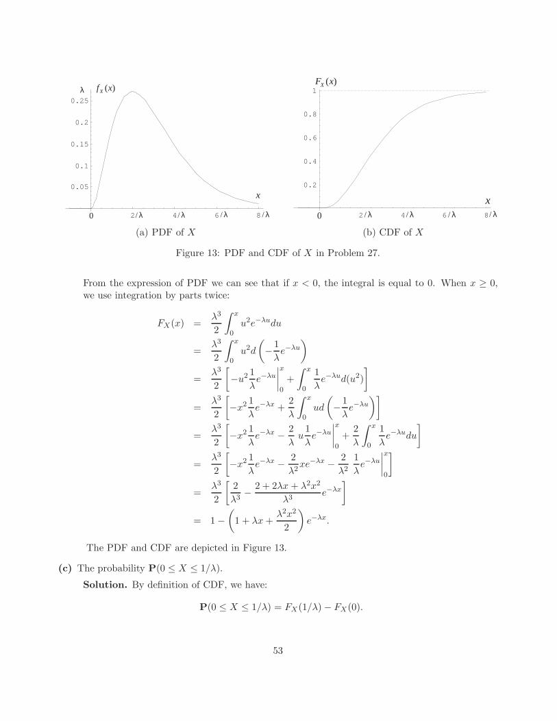
2 4 6 8
0.05
0.1
0.15
0.2
0.25
x
) ( x f X
λ / λ / λ / λ / 0
λ
2 4 6 8
0.2
0.4
0.6
0.8
1
x λ / λ / λ / λ /
) ( x F X
0
(a) PDF of X (b) CDF of X
Figure 13: PDF and CDF of X in Problem 27.
From the expression of PDF we can see that if x < 0, the integral is equal to 0. When x ≥ 0,we use integration by parts twice:
FX(x) =λ3
2
∫ x
0u2e−λudu
=λ3
2
∫ x
0u2d
(
− 1
λe−λu
)
=λ3
2
[
−u2 1
λe−λu
∣∣∣∣
x
0
+
∫ x
0
1
λe−λud(u2)
]
=λ3
2
[
−x2 1
λe−λx +
2
λ
∫ x
0ud
(
− 1
λe−λu
)]
=λ3
2
[
−x2 1
λe−λx − 2
λu
1
λe−λu
∣∣∣∣
x
0
+2
λ
∫ x
0
1
λe−λudu
]
=λ3
2
[
−x2 1
λe−λx − 2
λ2xe−λx − 2
λ2
1
λe−λu
∣∣∣∣
x
0
]
=λ3
2
[2
λ3− 2 + 2λx + λ2x2
λ3e−λx
]
= 1 −(
1 + λx +λ2x2
2
)
e−λx.
The PDF and CDF are depicted in Figure 13.
(c) The probability P(0 ≤ X ≤ 1/λ).
Solution. By definition of CDF, we have:
P(0 ≤ X ≤ 1/λ) = FX(1/λ) − FX(0).
53

-1 1 2 3 4 5
0.1
0.2
0.3
0.4
0.5
0.6
0.7 ) ( x f X
0 x
2
1
=
=
µ σ
Figure 14: Laplace PDF.
By plugging in 1/λ and 0 into the expression of CDF obtained in Part(b), we get:
FX(1/λ) = 1 − (1 + 1 + 1/2)e−1 = 1 − 5
2e,
FX(0) = 0,
P(0 ≤ X ≤ 1/λ) = FX(1/λ) = 1 − 5
2e≈ 0.08030.
Problem 28. Laplace Random Variable. (Ilya Pollak and Bin Ni.)A random variable X has probability density
fX(x) = Ce−√
2|x−µ|σ ,
where µ is a real number and σ is a positive real number. (This is a Laplace or double-sided exponentialdistribution.) Find
(a) The constant C.
Solution. Applying the normalization axiom,
1 =
∫ ∞
−∞fX(x)dx = C
∫ ∞
−∞e−
√2|x−µ|
σ dx
= 2C
∫ ∞
µe−
√2(x−µ)
σ dx (due to symmetry about µ)
=√
2σC
∫ ∞
0e−udu (u =
√2(x − µ)
σ)
=√
2σC
⇒ C =1√2σ
.
(b) The mean of X.
54

Solution. Applying the definition of expectation,
E[X] =
∫ ∞
−∞xfX(x)dx =
∫ ∞
−∞xCe−
√2|x−µ|
σ dx.
Making a change of variable u = x − µ, we have:
E[X] =
∫ ∞
−∞(u + µ)Ce−
√2|u|σ du
= C
∫ ∞
−∞ue−
√2|u|σ du
︸ ︷︷ ︸
0
+µ
∫ ∞
−∞Ce−
√2|u|σ du
︸ ︷︷ ︸
1= µ.
(c) The variance of X.
Solution. Applying the definition of variance,
var[X] =
∫ ∞
−∞(x − E[X])2fX(x)dx
=1√2σ
∫ ∞
−∞(x − µ)2e−
√2|x−µ|
σ dx
=1
2
∫ ∞
−∞u2
√2
σe−
√2|u|σ du
=
∫ ∞
0u2
√2
σe−
√2uσ du
= the second moment of an exponential r.v. with λ =
√2
σ
=2
(√2
σ
)2 = σ2.
Problem 29. Let X be a normal random variable with mean µ and variance σ2.
(a) Compute the probabilities
P(X ≤ µ + σ)
P(X ≤ µ − σ)
P(X ≤ µ + 2σ)
Solution. (Ilya Pollak and Bin Ni.)If we define random variable Y = (X−µ)/σ, then Y is a standard normal random variable—i.e.,
55

a normal random variable with zero mean and unit variance.
P(X ≤ µ + σ) = P
(X − µ
σ≤ 1
)
= P(Y ≤ 1) = Φ(1) ≈ 0.8413,
P(X ≤ µ − σ) = P
(X − µ
σ≤ −1
)
= P(Y ≤ −1) = Φ(−1) = 1 − Φ(1) ≈ 0.1587,
P(X ≤ µ + 2σ) = P
(X − µ
σ≤ 2
)
= P(Y ≤ 2) = Φ(2) ≈ 0.9772.
(b) Compute the probabilities
P(µ − σ ≤ X ≤ µ + σ)
P(µ − 2σ ≤ X ≤ µ + 2σ)
Solution
P(µ − σ ≤ X ≤ µ + σ) = P(X ≤ µ + σ) − P(X ≤ µ − σ)
≈ 0.8413 − 0.1587 = 0.6826,
P(µ − 2σ ≤ X ≤ µ + 2σ) = P(X ≤ µ + 2σ) − P(X ≤ µ − 2σ)
≈ 0.9772 − (1 − 0.9772) = 0.9544.
Problem 30. (Drake [2], problem 2.17. Solutions by Ilya Pollak and Bin Ni.)Stations A and B are connected by two parallel message channels. A message from A to B is sent overboth channels at the same time. Continuous random variables X and Y represent the message delays(in hours) over parallel channels I and II, respectively. These two random variables are independent,and both are uniformly distributed from 0 to 1 hours.
A message is considered “received” as soon as it arrives on any one channel, and it is considered“verified” as soon as it has arrived over both channels.
(a) Determine the probability that a message is received within 15 minutes after it is sent.
Solution. Because the marginal PDF’s are uniform and the X,Y are independent, the pair(X,Y ) is uniformly distributed in the unit square as depicted in Figure 15. The probability ofany event in this sample space is equal to its area. The event that “a message is received within15 minute” is equivalent to “X ≤ 1/4 or Y ≤ 1/4”, which corresponds to the shaded region inFigure 15(a). The probability of this event is equal to the area which is 7/16.
(b) Determine the probability that the message is received but not verified within 15 minutes afterit is sent.
Solution. This event is equivalent to “(X ≤ 1/4 and Y > 1/4) or (Y ≤ 1/4 and X > 1/4)”,which is depicted as the shaded region in Figure 15 (b). The probability of this event is equalto 3/16+3/16=3/8.
(c) Let T represent the time (in hours) between transmission at A and verification at B. Determinethe cumulative distribution function FT (t), and then differentiate it to obtain the PDF fT (t).
56

x
y
1
1
0
4/1
4/1
x
y
1
1
0
4/1
4/1
x
y
1
1
0
4/1
4/1
(a) (b) (d)
Figure 15: The events for Parts (a), (b), and (d) for Problem 30. The joint PDF of X and Y isuniform over the unit square.
Solution. By definition of CDF,
FT (t) = P(T ≤ t) = P(X ≤ t and Y ≤ t) = P(X ≤ t)P(Y ≤ t) (due to independence)
= FX(t)FY (t) =
0, t < 0,t2, 0 ≤ t ≤ 1,1, t > 1.
Differentiating, we get:
fT (t) =dFT (t)
dt=
{2t, 0 ≤ t ≤ 1,0, otherwise.
(d) If the attendant at B goes home 15 minutes after the message is received, what is the probabilitythat he is present when the message should be verified?
Solution. If he is present for verification, it means that the message arrived over one channelwithin 15 minutes of arriving over the other one: |X − Y | ≤ 1/4. This is illustrated in Figure15(d). The probability of this event is equal to 1 minus the area of the two triangles and we get:
P(|X − Y | ≤ 1/4) = 1 − (1 − 1/4)2 = 7/16.
(e) If the attendant at B leaves for a 15-minute coffee break right after the message is received, whatis the probability that he is present at the proper time for verification?
Solution. This event is equivalent to |X − Y | > 1/4. Its probability is:
1 − P(|X − Y | ≤ 1/4) = 9/16.
(f) The management wishes to have the maximum probability of having the attendant present at bothreception and verification. Would they do better to let him take his coffee break as describedabove or simply allow him to go home 45 minutes after transmission?
57

Solution. If the attendant is allowed to go home 45 minutes after the transmission, the prob-ability that he will be present at the both reception and verification is equal to the probabilitythat both messages arrive within 45 minutes. That is:
P(X ≤ 3/4 and Y ≤ 3/4) = (3/4)2 = 9/16.
This probability is equal to what we obtained in Part (e). So it does not matter which decisionthe manager will make in terms of maximizing the probability of the attendant’s presence atboth reception and verification. (But note that the coffee break strategy will keep the attendantat work for a longer time on average. Indeed, when the message is received more than 45 minutesafter the transmission, he will need to stay there for more than 45 minutes. In the second scheme,his working time is fixed to be 45 minutes.)
Problem 31. (Drake [2], Section 2-15, Example 2.)Each day he leaves home for the local casino, Oscar spins a biased wheel of fortune to determine howmuch money to take with him. He takes exactly X hundred dollars with him, where X is a continuousrandom variable described by the following probability density function:
fX(x) =
{x8 , 0 ≤ x ≤ 40, otherwise,
where x is in hundreds of dollars. As a matter of convenience, we are assuming that the currency isinfinitely divisible. (Rounding off to the nearest penny wouldn’t matter much.)
Oscar has a lot of experience at this. All of it is bad. Decades of experience have shown that, overthe course of an evening, Oscar never wins. In fact, the amount with which he returns home on anyparticular night is uniformly distributed between zero and the amount with which he started out.
Let the random variable Y represent the amount (in hundreds of dollars) Oscar brings home on anyparticular night.
(a) Determine fX,Y (x, y), the joint PDF for his original wealth X and his terminal wealth Y on anynight. Are X and Y independent? Present a convincing argument for your answer.
(b) Determine and plot fY (y), the marginal PDF for the amount Oscar will bring home on any night.
(c) Determine the expected value of Oscar’s loss on any particular night.
(d) On one particular night, we learn that Oscar returned home with less than $200. For that night,determine the conditional probability of each of the following events:
(i) He started out for the casino with less than $200.
(ii) His loss was less than $100.
(iii) His loss was exactly $75.
Solution.
58

0
fY |X(y|x)
xy
1
x
hundreds of dollars
x, initial capital inhundreds of dollars
y, terminal capital in
unity over the entire event space.that the calculated PDF does integrate toand zero elsewhere. A quick check showsJoint PDF is equal to 1/8 inside this triangle
4
40
(a) (b)
Figure 16: (a) Conditional PDF of Y given X. (b) The support of the joint PDF.
(a) From the problem statement we obtain:
fY |X(y|x) =
{1x , 0 ≤ y ≤ x ≤ 40, otherwise
This conditional density is shown in Fig. 16. This, in conjunction with the given fX(x), is usedto determine the joint PDF:
fX,Y (x, y) = fX(x)fY |X(y|x) =
{x8 · 1
x = 18 , 0 ≤ y ≤ x ≤ 4,
0, otherwise.
This result may be displayed in an x, y event space as shown in Fig. 16(b). If X and Y wereindependent, then the conditional density fY |X(y|x) would be equal to the marginal densityfY (y) of Y , and would not depend on the value x. It is, however, given that the conditionaldensity of Y given X = x is different for different values of x (specifically, it is uniform betweenzero and x). Therefore, X and Y are not independent.
0 4
y
4Event: y < Y ≤ y + dy
y
fy(y)
0.5
4.00
The PDF fY (y) does integrate to
to zero at y = 4decreasing from a maximum at y = 0that fY (y) must be linearlyunity. It can be seen from Fig. 1(b)
(a) (b)
Figure 17: (a) To obtain the marginal PDF of Y , integrate the joint PDF along the x-axis over thetriangular region. (b) The marginal PDF of Y .
(b) For 0 ≤ y ≤ 4,
fY (y) =
∫ ∞
−∞fX,Y (x, y)dx =
∫ 4
x=y
1
8dx =
1
8(4 − y).
59

This calculation and its result are illustrated in Fig. 17. Notice that the product of the marginaldensities of X and Y is not equal to the joint density of X and Y which was computed inPart (a). This is another way of seeing that X and Y are not independent.
(c)
E[X − Y ] =
∫
y
∫
x(x − y)fX,Y (x, y)dxdy
We must always be careful of the limits on the integrals when we substitute actual expressionsfor the joint PDF. We will integrate over x first.
E[X − Y ] =
∫ 4
y=0
∫ 4
x=y
1
8(x − y)dxdy =
∫ 4
y=0
[1
8
(x2
2− xy
)]x=4
x=y
dy
=
∫ 4
0
1
8
(
8 − 4y − y2
2+ y2
)
dy =
∫ 4
0
(
1 − y
2+
y2
16
)
dy
=
[
y − y2
4+
y3
48
]4
0
=4
3= $133.33.
Alternately, we can obtain E[X − Y ] as follows:
E[X − Y ] = E[X] − E[Y ] =
∫ ∞
x=−∞xfX(x)dx −
∫ ∞
y=−∞yfY (y)dy
=
∫ 4
0x · x
8dx −
∫ 4
0y · 4 − y
8dy
= $133.33
The event “he returned home with less than $200”y
x
2
4
40
Figure 18: The conditional sample space for Part (d).
(d) Given that Oscar returned home with less than $200, we work in the appropriate conditionalsample space. At all points consistent with the conditioning event, the conditional joint PDFis equal to the original joint PDF scaled up by the reciprocal of the a priori probability of theconditioning event. Since the original joint PDF is uniform, this means that the conditional jointPDF is also uniform. The area of the conditioning event is 6, therefore the conditional joint PDFgiven that Oscar returned with less than $200 is equal to 1
6 in the region where it is nonzero,i.e. the gray set in Fig. 18. Now we may answer all the questions in this conditional space.
60
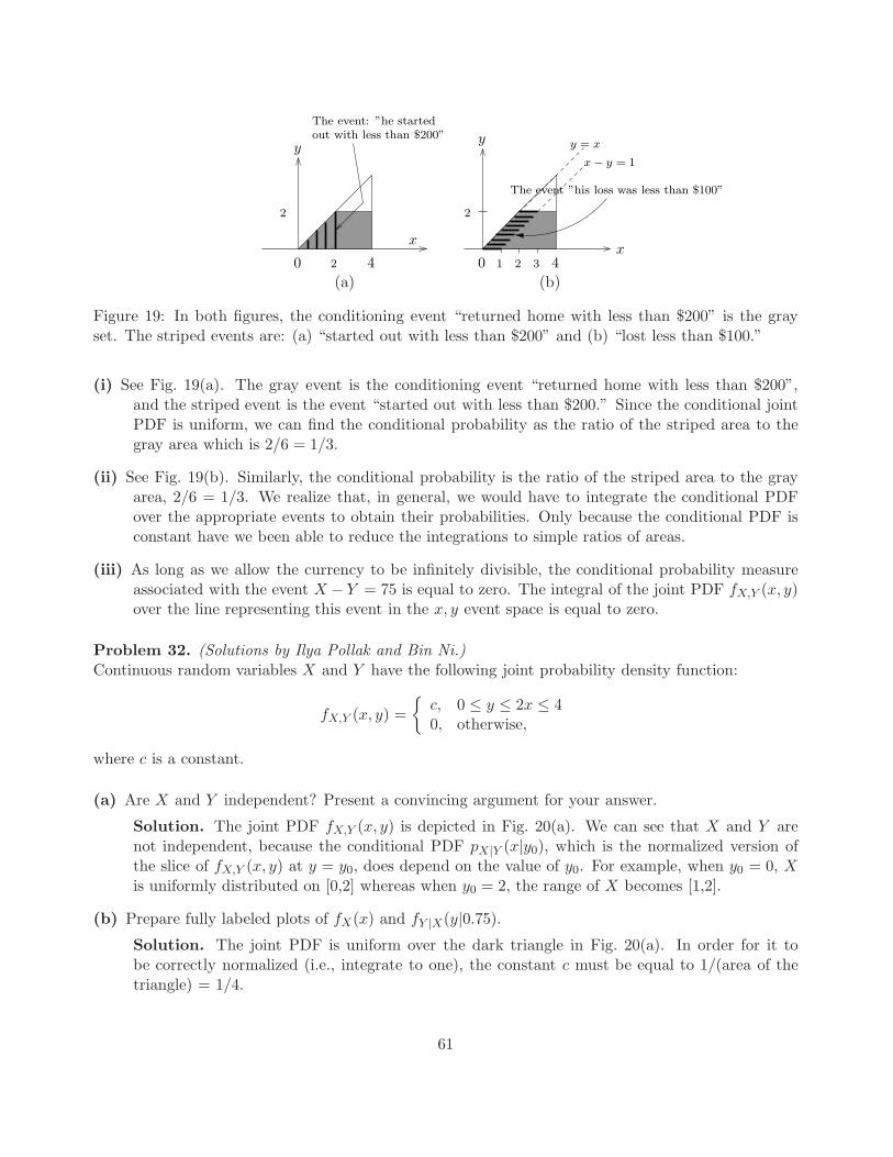
out with less than $200”The event: ”he started
y
x
20 4
2
0 4
2
21 3x
y = x
x − y = 1
y
The event ”his loss was less than $100”
(a) (b)
Figure 19: In both figures, the conditioning event “returned home with less than $200” is the grayset. The striped events are: (a) “started out with less than $200” and (b) “lost less than $100.”
(i) See Fig. 19(a). The gray event is the conditioning event “returned home with less than $200”,and the striped event is the event “started out with less than $200.” Since the conditional jointPDF is uniform, we can find the conditional probability as the ratio of the striped area to thegray area which is 2/6 = 1/3.
(ii) See Fig. 19(b). Similarly, the conditional probability is the ratio of the striped area to the grayarea, 2/6 = 1/3. We realize that, in general, we would have to integrate the conditional PDFover the appropriate events to obtain their probabilities. Only because the conditional PDF isconstant have we been able to reduce the integrations to simple ratios of areas.
(iii) As long as we allow the currency to be infinitely divisible, the conditional probability measureassociated with the event X − Y = 75 is equal to zero. The integral of the joint PDF fX,Y (x, y)over the line representing this event in the x, y event space is equal to zero.
Problem 32. (Solutions by Ilya Pollak and Bin Ni.)Continuous random variables X and Y have the following joint probability density function:
fX,Y (x, y) =
{c, 0 ≤ y ≤ 2x ≤ 40, otherwise,
where c is a constant.
(a) Are X and Y independent? Present a convincing argument for your answer.
Solution. The joint PDF fX,Y (x, y) is depicted in Fig. 20(a). We can see that X and Y arenot independent, because the conditional PDF pX|Y (x|y0), which is the normalized version ofthe slice of fX,Y (x, y) at y = y0, does depend on the value of y0. For example, when y0 = 0, Xis uniformly distributed on [0,2] whereas when y0 = 2, the range of X becomes [1,2].
(b) Prepare fully labeled plots of fX(x) and fY |X(y|0.75).Solution. The joint PDF is uniform over the dark triangle in Fig. 20(a). In order for it tobe correctly normalized (i.e., integrate to one), the constant c must be equal to 1/(area of thetriangle) = 1/4.
61
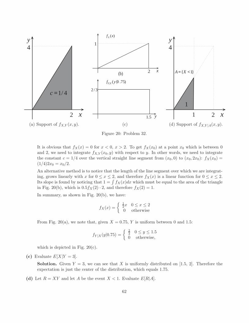
x
y 4
2
4 / 1 = c
x
) ( x f X
2
1
y
) 75 . 0 | ( | y f X Y
5 . 1
3 / 2
(b)
x
y 4
2
1
1
} 1 { < = X A
(a) Support of fX,Y (x, y). (c) (d) Support of fX,Y |A(x, y).
Figure 20: Problem 32.
It is obvious that fX(x) = 0 for x < 0, x > 2. To get fX(x0) at a point x0 which is between 0and 2, we need to integrate fX,Y (x0, y) with respect to y. In other words, we need to integratethe constant c = 1/4 over the vertical straight line segment from (x0, 0) to (x0, 2x0): fX(x0) =(1/4)2x0 = x0/2.
An alternative method is to notice that the length of the line segment over which we are integrat-ing, grows linearly with x for 0 ≤ x ≤ 2, and therefore fX(x) is a linear function for 0 ≤ x ≤ 2.Its slope is found by noticing that 1 =
∫fX(x)dx which must be equal to the area of the triangle
in Fig. 20(b), which is 0.5fX(2) · 2, and therefore fX(2) = 1.
In summary, as shown in Fig. 20(b), we have:
fX(x) =
{12x 0 ≤ x ≤ 20 otherwise
From Fig. 20(a), we note that, given X = 0.75, Y is uniform between 0 and 1.5:
fY |X(y|0.75) =
{23 0 ≤ y ≤ 1.50 otherwise,
which is depicted in Fig. 20(c).
(c) Evaluate E[X|Y = 3].
Solution. Given Y = 3, we can see that X is uniformly distributed on [1.5, 2]. Therefore theexpectation is just the center of the distribution, which equals 1.75.
(d) Let R = XY and let A be the event X < 1. Evaluate E[R|A].
62
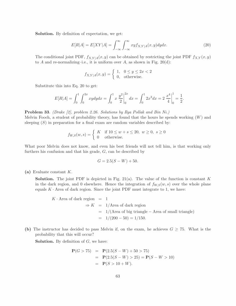
Solution. By definition of expectation, we get:
E[R|A] = E[XY |A] =
∫ ∞
−∞
∫ ∞
−∞xyfX,Y |A(x, y)dydx. (20)
The conditional joint PDF, fX,Y |A(x, y) can be obtained by restricting the joint PDF fX,Y (x, y)to A and re-normalizing–i.e., it is uniform over A, as shown in Fig. 20(d):
fX,Y |A(x, y) =
{1, 0 ≤ y ≤ 2x < 20, otherwise.
Substitute this into Eq. 20 to get:
E[R|A] =
∫ 1
0
∫ 2x
0xydydx =
∫ 1
0x
y2
2
∣∣∣∣
2x
0
dx =
∫ 1
02x3dx = 2
x4
4
∣∣∣∣
1
0
=1
2.
Problem 33. (Drake [2], problem 2.26. Solutions by Ilya Pollak and Bin Ni.)Melvin Fooch, a student of probability theory, has found that the hours he spends working (W ) andsleeping (S) in preparation for a final exam are random variables described by:
fW,S(w, s) =
{K if 10 ≤ w + s ≤ 20, w ≥ 0, s ≥ 00 otherwise.
What poor Melvin does not know, and even his best friends will not tell him, is that working onlyfurthers his confusion and that his grade, G, can be described by
G = 2.5(S − W ) + 50.
(a) Evaluate constant K.
Solution. The joint PDF is depicted in Fig. 21(a). The value of the function is constant Kin the dark region, and 0 elsewhere. Hence the integration of fW,S(w, s) over the whole planeequals K · Area of dark region. Since the joint PDF must integrate to 1, we have:
K · Area of dark region = 1
⇒ K = 1/Area of dark region
= 1/(Area of big triangle − Area of small triangle)
= 1/(200 − 50) = 1/150.
(b) The instructor has decided to pass Melvin if, on the exam, he achieves G ≥ 75. What is theprobability that this will occur?
Solution. By definition of G, we have:
P(G > 75) = P(2.5(S − W ) + 50 > 75)
= P(2.5(S − W ) > 25) = P(S − W > 10)
= P(S > 10 + W ).
63

w
s 20
20 10
10 K
w
s 20
20 10
10
w s + = 10
w s + = 10 -
D
E
F
O
20 - 5 . 2
g
w g
s l + = 20 - 5 . 2
:
(a) FW,S(w, s) (b)
20 40 60 80 100
0.2
0.4
0.6
0.8
1
g
) ( g F G
g
) ( g f G
20 40 60 80 100
0.002
0.004
0.006
0.008
0.01
0.012
(c) FG(g) (d) fG(g)
Figure 21: Illustrations for Problem 3.
64

The event A = {S > 10 + W} corresponds to the semi-infinite plane above the upper dashedline in Fig. 21(b). By definition of PDF, we have:
P(A) =
∫ ∫
(s,w)∈A
fW,S(w, s)dwds
= K · Area of DEF =1
150· 25 =
1
6
(c) Make a neat and fully labeled sketch of the probability density function fG(g).
Solution. Given the range of W and S, it’s not hard to check that G ranges from 0 to 100.Therefore fG(g) = 0 for g < 0, g > 100. For 0 ≤ g ≤ 100, it will be easier to get the CDF firstand then take derivative. By definition of CDF, we have:
FG(g) = P(G < g) = P(
S − W <g
2.5− 20
)
(21)
= P(
S <g
2.5− 20 + W
)
. (22)
Similarly to the last part, P(S < g
2.5 − 20 + W)
equals K times the area of the piece of the darkregion below the straight line l : s < g
2.5 − 20 + w which is depicted in Fig. 21(b). Because of theshape of the dark region, Eq. 22 needs to be evaluated under three cases:
Case 1. −20 ≤ g2.5 − 20 < −10, which is equivalent to 0 ≤ g < 25:
In this case, l is below the lower dashed line in the figure, and so the area of interest is:
A(g) =1
4
( g
2.5
)
=g2
25,
and therefore
FG(g) = KA(g) =g2
3750.
Case 2. −10 ≤ g2.5 − 20 < 10, which is equivalent to 25 ≤ g < 75:
In this case, l is between the lower dashed line and the upper dashed line in the figure, andso
A(g) = 5( g
2.5− 10
)
+ 25 = 2g − 25,
and
FG(g) = KA(g) =2g − 25
150.
Case 3. 10 ≤ g2.5 − 20 ≤ 20, which is equivalent to 75 ≤ g ≤ 100:
In this case, l is above the upper dashed line in the figure, and so
A(g) = 150 − 1
4
(
40 − g
2.5
)2= 8g − g2
25− 250,
and
FG(g) = KA(g) =8g − g2/25 − 250
150.
65

w
s 20
20 10 O
20 - /2.5 g
w g
s l + = 20 - 5 . 2
:
20 - /2.5 ) ( g g ∆ +
w g g
s l + +
= 20 - 5 . 2
: 1
∆
2 5 . 2
g ∆
Figure 22: Problem 3(c), alternative method.
Combining the three cases, FG(g) is depicted as in Fig. 21(c). If we differentiate, we’ll get:
fG(g) =
g/1875 0 ≤ g < 251/75 25 ≤ g < 75
4/75 − g/1875 75 ≤ g ≤ 1000 otherwise,
which is depicted in Figure 21(d).
Another way to solve this problem is based on the following fact:
fG(g) =dFG(g)
dg= lim
∆g→0
FG(g + ∆g) − FG(g)
∆g.
As depicted in Fig. 22, FG(g +∆g)−FG(g) is equal to the probability of the black region, whichis the part of the dark region between straight line l and l1 : s = g+∆g
2.5 − 20 + w. When ∆g is
small, the area of the black region can be approximated by ∆g
2.5√
2times the length of the segment
of line l that is cut by the dark region. Therefore we have:
fG(g) = K1
2.5√
2· length of the segment of line l that is cut by the dark region
When 0 ≤ g ≤ 25 it is linearly increasing, when 25 ≤ g ≤ 75 it is constant, and when 75 ≤ g ≤100 it is linearly decreasing. It is therefore a trapezoid, as shown in Fig. 21(d). The lengths of
66

the two parallel sides are 100, 50 respectively. The height of the trapezoid equals:
fG(25) = K1
2.5√
2· 10√
2=
1
75
It can also be found according to the normalization axiom:
100 + 50
2fG(25) = 1
⇒ fG(25) =1
75.
(d) Melvin, true to form, got a grade of exactly 75 on the exam. Determine the conditional probabilitythat he spent less than one hour working in preparation for this exam.
Solution. Given that he got a 75, the set of possible outcomes is just segment EF in Fig. 21(b).Since the joint PDF is constant on the set, the conditional density of W is uniform on [0,5], andP(W < 1|G = 75) = 1/5.
References
[1] D.P. Bertsekas and J.N. Tsitsiklis. Introduction to Probability, 2nd Edition, Athena Scientific, Belmont, Mas-sachusetts, 2008.
[2] A. Drake. Fundamentals of Applied Probability Theory, McGraw-Hill, Inc., 1988.
[3] A. Leon-Garcia. Probability and Random Processes for Electrical Engineering, 2nd Edition, Addison Wesley Long-man, 1994.
[4] J. Montier. Behavioural Investing: A Practitioners Guide to Applying Behavioural Finance. Wiley, 2007.
[5] Q.F. Stout and B. Warren. Tree algorithms for unbiased coin tossing with a biased coin. The Annals of Probability,
12(1):212–222, Feb. 1984.
67