ece 1010 ece problem solving i solutions to 5 systems of

ECE 1010 ECE Problem Solving I

Chapter 5: Overview 5–1

Solutions to Systems of Linear EquationsOverview

In this chapter we studying the solution of sets of simultaneouslinear equations using matrix methods. The first section consid-ers the graphical interpretation of such solutions.

Graphical Interpretation

• In engineering problem solving the need to solve a set ofsimultaneous linear equations arises frequently

– Note: We keep specializing the system of equations to lin-ear equations since in the modeling of large systems, lin-ear approximations are a reasonable first approach and inmany cases sufficient for design purposes

• To develop an appreciation for what is really happening whenwe ask the computer solve a set of simultaneous linear equa-tions, we will explore graphical solutions first

5


Chapter 5: Graphical Interpretation 5–2

A Pair of Linear Equations with Two Unknowns

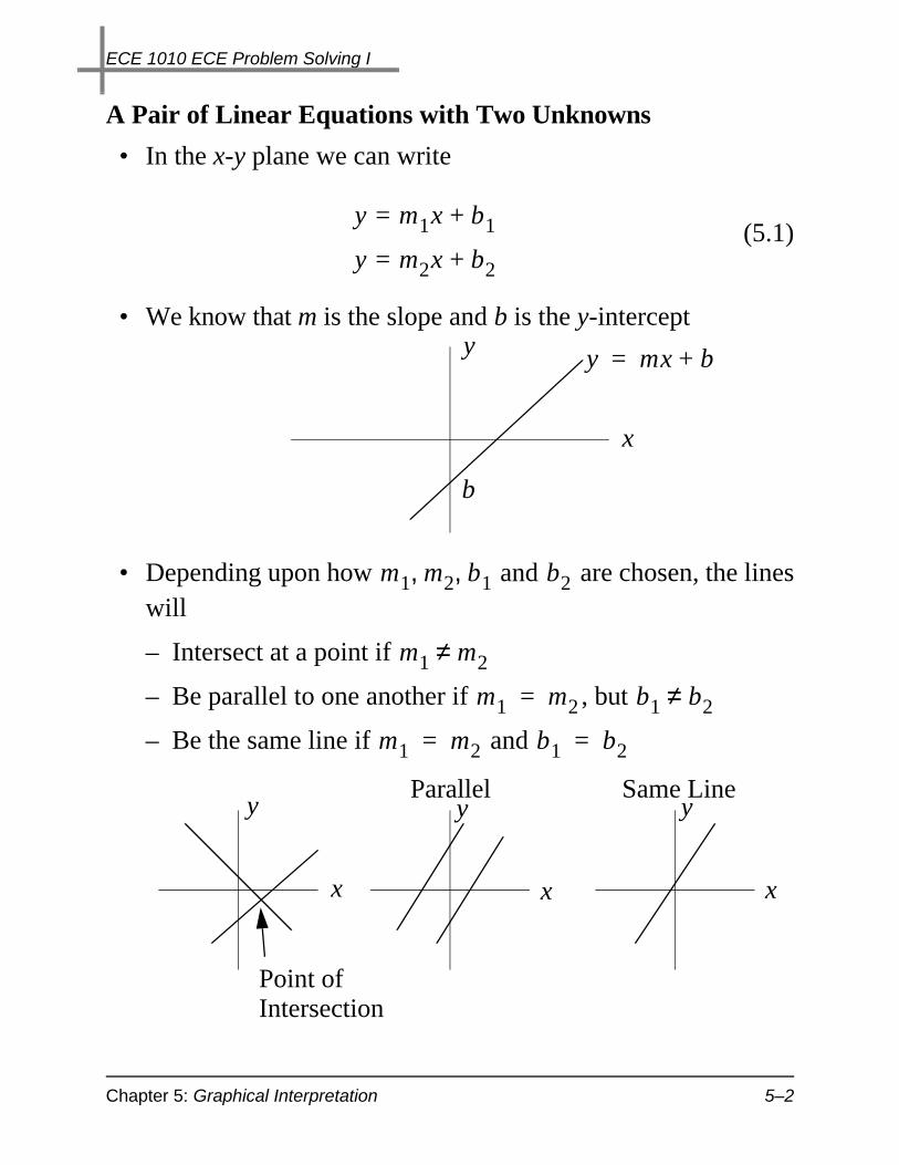
• In the x-y plane we can write

(5.1)

• We know that m is the slope and b is the y-intercept

• Depending upon how are chosen, the lineswill

– Intersect at a point if

– Be parallel to one another if , but

– Be the same line if and

y m1x b1+=

y m2x b2+=

x

y y mx b+=

b

m1 m2 b1 and b2, ,

m1 m2≠

m1 m2= b1 b2≠

m1 m2= b1 b2=

Point ofIntersection

Parallel Same Line

x

y

x

y

x

y



• To obtain a matrix formulation of this problem we would firstrewrite (5.1) as

(5.2)

or

(5.3)

• The two lines intersect in a point if the matrix inverse

(5.4)

exists; why?

• Consider

m1x y– b1–=

m2x y– b2–=

m1 1–

m2 1–

x

y

b1–

b2–=

m1 1–

m2 1–

1–

m1 1–

m2 1–

1–m1 1–

m2 1–

x

y

m1 1–

m2 1–

1–b1–

b2–=

1 0

0 1I=



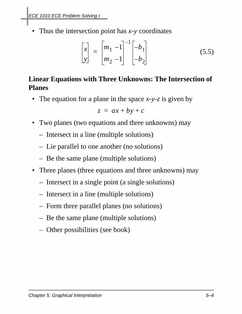
• Thus the intersection point has x-y coordinates

(5.5)

Linear Equations with Three Unknowns: The Intersection of Planes

• The equation for a plane in the space x-y-z is given by

• Two planes (two equations and three unknowns) may

– Intersect in a line (multiple solutions)

– Lie parallel to one another (no solutions)

– Be the same plane (multiple solutions)

• Three planes (three equations and three unknowns) may

– Intersect in a single point (a single solutions)

– Intersect in a line (multiple solutions)

– Form three parallel planes (no solutions)

– Be the same plane (multiple solutions)

– Other possibilities (see book)

x

y

m1 1–

m2 1–

1–b1–

b2–=

z ax by c+ +=



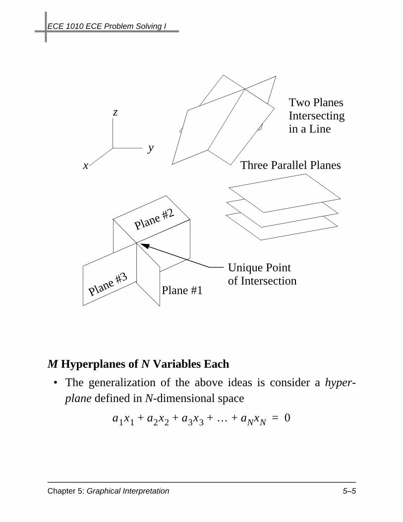
M Hyperplanes of N Variables Each

• The generalization of the above ideas is consider a hyper-plane defined in N-dimensional space

y

x

z

Plane #1

Plane #2

Plane #3Unique Pointof Intersection

Three Parallel Planes

Two PlanesIntersectingin a Line

a1x1 a2x2 a3x3 … aNxN+ + + + 0=



• We can not actually draw hyperplanes beyond , butthe concept of solving M simultaneous equations of Nunknowns, extends from the notions developed for threedimensions

• In the following assume the M hyperplanes are unique

• If we say that the system is underspecified and aunique solution does not exist

– As an example consider how two planes may intersect in aline (here and )

• If a unique solution is possible if none of the hyper-planes are parallel to each other

– As an examples consider how three faces of a cube inter-sect in a point

• If we say that the system is overspecified and a uniquesolution does not exist

– As an example consider how three lines in the plane maypair-wise intersect, but not have a common solution

• When a unique solution exists we say that the system ofequations is nonsingular

• When no unique solution exists we say the system of equa-tions is singular

N 3=

M N<

M 2= N 3=

M N=

M N>


Chapter 5: Solutions Using Matrix Operations 5–7

Solutions Using Matrix Operations

• The two equations and two unknowns given in (5.2) can becast into a more general notation as follows

• Extending to N equations and N unknowns we have

(5.6)

• If we let

(5.7)

we can write (5.6) in matrix form

(5.8)

• Not that we could also write (5.6) as

(5.9)

a11x1 a12x2+ b1=

a21x1 a22x2+ b2=

a11x1 a12x2 … a1NxN+ + + b1=

a21x1 a22x2 … a2NxN+ + + b2=

…aN1x1 aN2x2 … aNNxN+ + + bN=

A

a11 a12 … a1N

a21 a22 … …

… … … …aN1 … … aNN

X,

x1

x2

…xN

B,

b1

b2

…bN

= = =

AX B=

XTA

TB

T=



• This follows from the matrix theory result that

– Note: (5.9) is simply another way expressing a system of Nequations and N unknowns as a matrix equation

Matrix Division

• In MATLAB solving matrix equations of the form (5.8) and(5.9) is very easy

• Two basic approaches are available

• In this subsection we consider the use of matrix division

• Given

(the form of (5.8)) is the matrix equation, with X the quantityof interest, we use matrix left division as follows

X = A\B; % Note the backslash

– The numerical technique used here is Gauss elimination

• Given

(the form of (5.8)) is the matrix equation, with X the quantityof interest, we use matrix right division as follows

X = A/B; % Note the backslash

Example: N = 2

» A = [1 2; 3 4];

» B = [2; 5];

» X = A\B

GH( )TH

TG

T=

AX B=

XA B=



X =

1.0000

0.5000

» Xt = B'/A'

Xt =

1.0000 0.5000 %The same solutions as expected

• If the solution is singular MATLAB gives Nan’s or Inf’s

• If the solution is nearly singular, a warning message is given

Matrix Inverse

• As shown in (5.5) an alternate solution approach involves theuse of the matrix inverse, i.e., if

then

but and , so

(5.10)

• In MATLAB this would be written asX = inv(A)*B;

AX B=

A1–AX A

1–B=

A1–A I= IX X=

X A1–B=



• Using (5.9) the solution is

which reduces to

(5.11)

Example: Practice! p. 157 (2,6)

Solve the following systems of equations using both matrix divi-sion and inverse matrices. For systems with just two variables(unknowns), plot the equations on the same graph to see theintersection (unique solution) or show that the system is singular(without a unique solution).

2. A system of two equations and two unknowns:

• Load the system into MATLAB with

» A = [-2 1; -2 1]; B = [-3; 1];

» % Solve using matrix division:

» X = A\B

Warning: Matrix is singular to working precision.

XTA

TA

T( )1–

BT

AT( )

1–=

XT

BT

AT( )

1–=

2x1– x2+ 3–=

2– x1 x2+ 1=

A 2– 12– 1

B, 3–1

= =



X =

Inf

Inf

» % Solve using the matrix inverse, first check

» % to see if rank is 2

» rank(A)

ans = 1

» % Unique solution does not exist

• Now we plot the two equations to see what is going on withregard to the solution

» x1 = -10:.1:10;

» x2_1 = 2*x1 - 3;

» x2_2 = 2*x1 + 1;

» s = length(x1);

» plot(x1(1:10:s),x2_1(1:10:s),'s',x1(1:10:s),...

x2_2(1:10:s),'d')% Plot symbols at a few points

» legend('First Eqn','Second Eqn')

» hold

Current plot held

» plot(x1,x2_1,x1,x2_2) % Plot lines with all points

» grid

» title('Plot of Two Equations for #2','fontsize',16)

» ylabel('x2','fontsize',14)

» xlabel('x1','fontsize',14)



6. A system of three equations and three unknowns:

-10 -8 -6 -4 -2 0 2 4 6 8 10-25

-20

-15

-10

-5

0

5

10

15

20

25Plot of Two Equations for #2

x2

x1

First Eqn Second Eqn

3x1 2x2 x3–+ 1=

x1– 3x2 2x3+ + 1=

x1 x2– x3– 1=



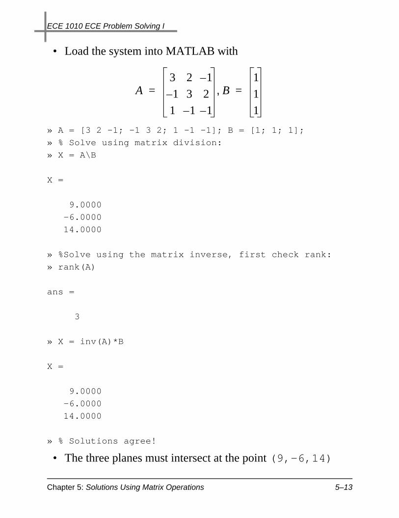
• Load the system into MATLAB with

» A = [3 2 -1; -1 3 2; 1 -1 -1]; B = [1; 1; 1];

» % Solve using matrix division:

» X = A\B

X =

9.0000

-6.0000

14.0000

» %Solve using the matrix inverse, first check rank:

» rank(A)

ans =

3

» X = inv(A)*B

X =

9.0000

-6.0000

14.0000

» % Solutions agree!

• The three planes must intersect at the point (9,-6,14)

A3 2 1–

1– 3 2

1 1– 1–

B,1

1

1

= =


Chapter 5: Problem Solving Applied: Electrical Circuit Analysis 5–14

Problem Solving Applied: Electrical Circuit Analysis

In the solution of electrical circuit problems we must deal withsystems of linear equations. The electrical engineering curricu-lum does not take this subject lightly.

– The electrical engineering BSEE program devotes twosemesters to circuit analysis

– Two semesters to electronic circuits analysis

– One semester to the study of signals and systems

• The foundation of circuit analysis are Kirchoff’s voltage andcurrent laws

• We will briefly introduce these two laws here, but to keepthings simple we will only consider resistor networks withdirect current (dc) or ideal battery sources

Kirchoff’s Voltage Law

The sum of voltage drops (or rises) around a closed loop in a cir-cuit (without any independent current sources in series) is zero.

• The voltage drop across a resistive element is the currentthrough the element times the element resistance, e.g. ohmslaw

R

iv+ -

v iR=Ohms Law



A simple application:

• Kirchoff’s voltage law applied to the single loop current gives

or

Kirchoff’s Current Law

The sum of currents leaving (or entering) a node in a circuit(without any independent voltage sources attached) is zero.

• Again ohm’s law comes in handyA Simple Example:

v1+-

R1R2

i1

++ -

-

i1

v1– R1i1 R2i1+ + 0=

R1 R2+( )i1 v1=

v1+-

R1R2

+

-

v2



• Kirchoff’s current law applied to node voltage gives

or

(assume is known)

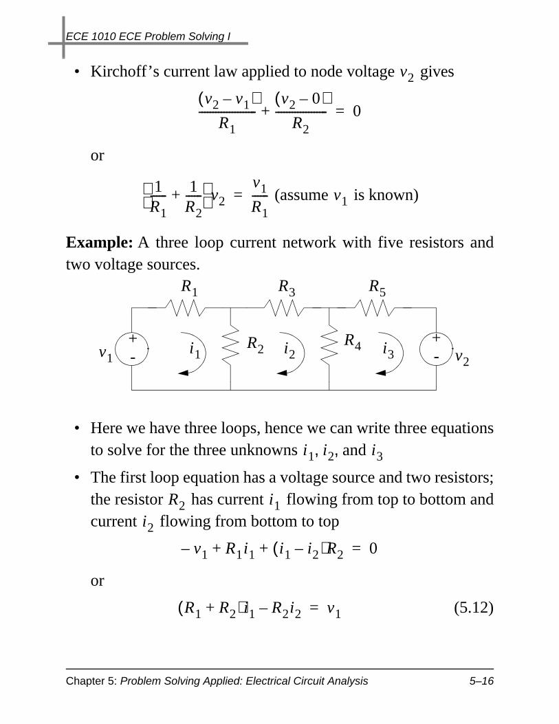
Example: A three loop current network with five resistors andtwo voltage sources.

• Here we have three loops, hence we can write three equationsto solve for the three unknowns

• The first loop equation has a voltage source and two resistors;the resistor has current flowing from top to bottom andcurrent flowing from bottom to top

or

(5.12)

v2

v2 v1–( )R1

---------------------v2 0–( )

R2-------------------+ 0=

1R1------ 1

R2------+

v2

v1

R1------= v1

v1

+-

+- v2

R1 R3 R5

R2R4i2i1 i3

i1 i2 and i3, ,

R2 i1i2

v1– R1i1 i1 i2–( )R2+ + 0=

R1 R2+( )i1 R2i2– v1=



• The second loop equation involves three resistors, but allthree loop currents appear in the equation

or

(5.13)

• The third loop equation as with the first involves a voltagesource and two resistors

or

(5.14)

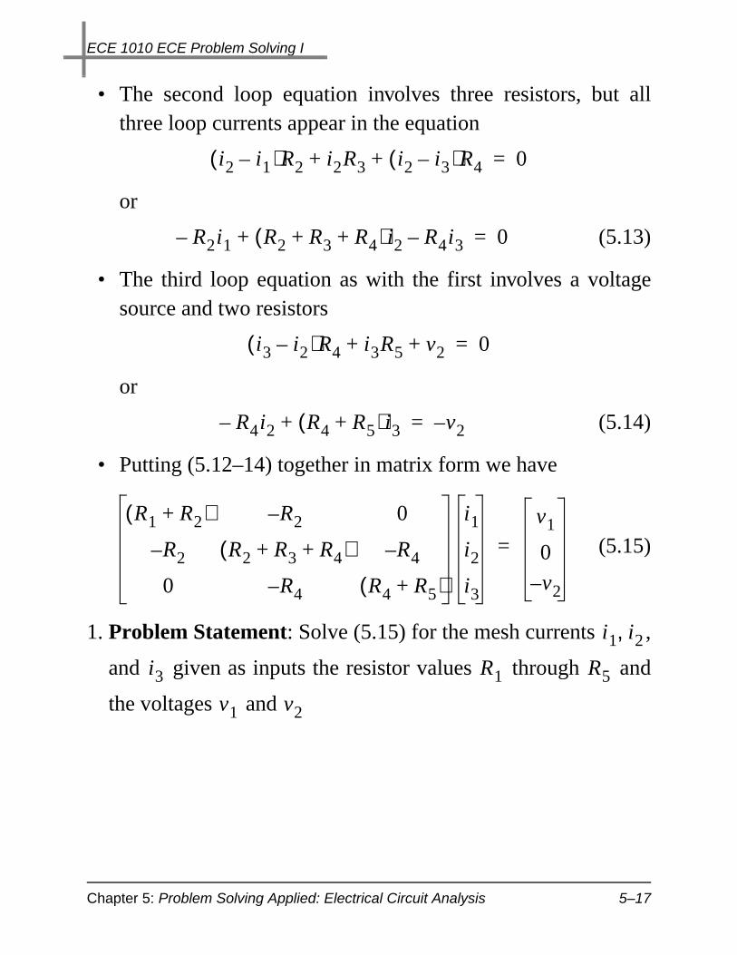
• Putting (5.12–14) together in matrix form we have

(5.15)

1. Problem Statement: Solve (5.15) for the mesh currents ,

and given as inputs the resistor values through and

the voltages and

i2 i1–( )R2 i2R3 i2 i3–( )R4+ + 0=

R2i1– R2 R3 R4+ +( )i2 R4i3–+ 0=

i3 i2–( )R4 i3R5 v2+ + 0=

R4i2– R4 R5+( )i3+ v2–=

R1 R2+( ) R2– 0

R2– R2 R3 R4+ +( ) R4–

0 R4– R4 R5+( )

i1

i2

i3

v1

0

v2–

=

i1 i2,

i3 R1 R5

v1 v2



2. Input/Output Description: The I/O diagram is shown below

3. Hand Calculation: For a hand calculation assume that

ohm

and

• We must solve

• We solve this using MATLAB’s left division command andthen check the solution by computing the error

» A = [2 -1 0; -1 3 -1; 0 -1 2];

» B = [5; 0; 6];

» X = A\B

X =

3.8750 % Units of amps



MA

TL

AB

Solu

tion

MeshCurrents

ResistorValues

VoltageSourceValues

R1 R2 R3 R4 R5 1= = = = =

v1 5 volts= v2 6– volts=

2 1– 0

1– 3 1–

0 1– 2

i1

i2

i3

5

0

6

=



» Error = sum(A*X-B)

Error = -2.6645e-015 % Very small

4. MATLAB Solution: A script will be written which promptsthe user to supply the five resistor values followed by the twovoltage values.

% Three-loop Circuit, three_loop.m

% Five resistors and two voltage sources

%

% Prompt user to enter resistor values:

R = input('Enter [R1 R2 ... R5] in ohms--> ');

% Prompt user to enter voltage source values:

V = input('Enter voltage values [v1 v2] in volts--> ');

% Fill the A matrix and the B vector:

A = [R(1)+R(2) -R(2) 0;

-R(2) R(2)+R(3)+R(4) -R(4);

0 -R(4) R(4)+R(5)];

B = [V(1); 0; -V(2)];

% Make sure solution is not singular

if rank(A) == 3

fprintf('The mesh currents in amps are: \n');

i = A\B

else

fprintf('The solution is not unique');

end

% Were Done!



5. Test Results:

• First check out the hand calculated value» three_loop

Enter [R1 R2 ... R5] in ohms--> [1 1 1 1 1]

Enter voltage values [v1 v2] in volts--> [5 -6]

The mesh currents in amps are:

i =

3.8750

2.7500 <<--Values all agree with hand calculation

4.3750

• Try different resistor values and turn voltage source off.» three_loop

Enter [R1 R2 ... R5] in ohms--> [2 3 2 3 2]

Enter voltage values [v1 v2] in volts--> [5 0]

The mesh currents in amps are:

i =

1.4091

0.6818 % All currents in amps

0.4091

» % Check the solution error

» Error = sum(A*i-B) % better check sum(abs(A*i-B))

Error =

1.1102e-015 % Small so solution seems reasonable

v2



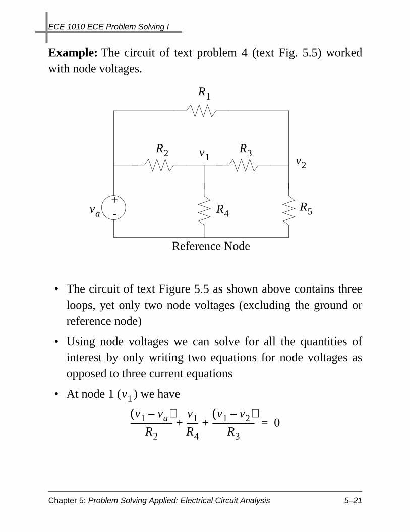
Example: The circuit of text problem 4 (text Fig. 5.5) workedwith node voltages.

• The circuit of text Figure 5.5 as shown above contains threeloops, yet only two node voltages (excluding the ground orreference node)

• Using node voltages we can solve for all the quantities ofinterest by only writing two equations for node voltages asopposed to three current equations

• At node 1 ( ) we have

+-va

v1 v2

R1

R2 R3

R4R5

Reference Node

v1

v1 va–( )R2

---------------------v1

R4------

v1 v2–( )R3

---------------------+ + 0=



or

(5.16)

• At node 2 ( ) we have

or

(5.17)

• In matrix form (5.16) and (5.17) become

(5.18)

1R2------ 1

R3------ 1

R4------+ +

v11

R3------v2–

va

R2------=

v2

v2 va–( )R1

---------------------v2 v1–( )

R3---------------------

v2

R5------+ + 0=

1R3------v1– 1

R1------ 1

R3------ 1

R5------+ +

v2+va

R1------=

1R2------ 1

R3------ 1

R4------+ +

1R3------–

1R3------– 1

R1------ 1

R3------ 1

R5------+ +

v1

v2

va

R2------

va

R1------

=

ece 1010 ece problem solving i solutions to 5 systems of

Documents