ebbr instrument handbook

DOE/SC-ARM-TR-037

Energy Balance Bowen Ratio (EBBR) Instrument Handbook

August 2017

DR Cook

DISCLAIMER

This report was prepared as an account of work sponsored by the U.S. Government. Neither the United States nor any agency thereof, nor any of their employees, makes any warranty, express or implied, or assumes any legal liability or responsibility for the accuracy, completeness, or usefulness of any information, apparatus, product, or process disclosed, or represents that its use would not infringe privately owned rights. Reference herein to any specific commercial product, process, or service by trade name, trademark, manufacturer, or otherwise, does not necessarily constitute or imply its endorsement, recommendation, or favoring by the U.S. Government or any agency thereof. The views and opinions of authors expressed herein do not necessarily state or reflect those of the U.S. Government or any agency thereof.

DOE/SC-ARM-TR-037

Energy Balance Bowen Ratio (EBBR) Instrument Handbook DR Cook, Argonne National Laboratory August 2017 Work supported by the U.S. Department of Energy, Office of Science, Office of Biological and Environmental Research

DR Cook, August 2017, DOE/SC-ARM-TR-037

iii

Acronyms and Abbreviations

AC Alternating Current AEM automatic exchange mechanism AERI atmospheric emitted radiance interferometer ARM Atmospheric Radiation Measurement BA Bulk Aerodynamic Technique C Celsius CF Central Facility cm centimeter DC Direct Current DQ Explorer Data Quality Explorer DQO Data Quality Office DQR Data Quality Report EBBR energy balance Bowen ratio ECMWF European Center for Medium Range Weather Forecasts ECOR Eddy Correlation System EF Extended Facility EFSCO Extended Facility Surface Conditions Observations FIFE First ISLSCP Field Experiment GCIP GEWEX Continental-Scale International Project GEWEX Global Energy and Water cycle Exchanges IMMS Instrument Mentor Monthly Summary IRT infrared thermometer ISLCP International Satellite Land surface Climatology Project kPa kilopascal m meter MET surface meteorological instrumentation mV millivolt NIST National Institute of Standards and Technology OMIS Operations Management Information System PILPS Project for Intercomparison of Land-surface Schemes PRTD platinum resistance temperature detector QC quality control QME Quality Measurement Experiment REBS Radiation and Energy Balance Systems, Inc. RH relative humidity


iv

RMSE root-mean-square error SEBS Surface Energy Balance System SGP Southern Great Plains SIRS Solar and Infrared Station SWATS Soil Water and Temperature System VAP value-added product


v

Contents

Acronyms and Abbreviations ...................................................................................................................... iii 1.0 General Overview ................................................................................................................................. 7 2.0 Contacts ................................................................................................................................................ 7

2.1 Mentor .......................................................................................................................................... 7 2.2 Instrument Developer ................................................................................................................... 7

3.0 Deployment Locations and History ...................................................................................................... 7 4.0 Near-Real-Time Data Plots .................................................................................................................. 8 5.0 Data Description and Examples ........................................................................................................... 9

5.1 Data File Contents ........................................................................................................................ 9 5.1.1 Primary Variables and Expected Uncertainty ................................................................... 9 5.1.2 Secondary/Underlying Variables .................................................................................... 10 5.1.3 Diagnostic Variables ....................................................................................................... 11 5.1.4 Data Quality Flags ........................................................................................................... 11 5.1.5 Dimension Variables ....................................................................................................... 12

5.2 Annotated Examples .................................................................................................................. 12 5.3 User Notes and Known Problems .............................................................................................. 14 5.4 Frequently Asked Questions ...................................................................................................... 14

6.0 Data Quality ........................................................................................................................................ 19 6.1 Data Quality Health and Status .................................................................................................. 19 6.2 Data Reviews by Instrument Mentor.......................................................................................... 19 6.3 Data Assessments by Site Scientist/Data Quality Office ........................................................... 20 6.4 VAPS and Quality Measurement Experiments (QMEs) ............................................................ 23

7.0 Instrument Details............................................................................................................................... 23 7.1.1 List of Components ......................................................................................................... 23 7.1.2 System Configuration and Measurement Methods ......................................................... 24 7.1.3 Specifications .................................................................................................................. 24

7.2 Theory of Operation ................................................................................................................... 25 7.3 Calibration .................................................................................................................................. 27

7.3.1 Theory ............................................................................................................................. 27 7.3.2 Procedures ....................................................................................................................... 27 7.3.3 History ............................................................................................................................. 27

7.4 Operation and Maintenance ....................................................................................................... 27 7.4.1 User Manual .................................................................................................................... 27 7.4.2 Routine and Corrective Maintenance Documentation .................................................... 27 7.4.3 Software Documentation ................................................................................................. 28 7.4.4 Additional Documentation .............................................................................................. 28


vi

7.5 Glossary ...................................................................................................................................... 28 8.0 Citable References .............................................................................................................................. 28 9.0 Bibliography ....................................................................................................................................... 29

Figures

1 Plot showing sensible (h) and latent (e) heat fluxes showing a normal diurnal variation in heat fluxes. ................................................................................................................................................... 13

2 Plot showing the spiked data replaced by the BA EBBR VAP with fluxes calculated with the BA................................................................................................................................................... 13

Tables

1 EBBR status. .......................................................................................................................................... 7


7

1.0 General Overview The energy balance Bowen ratio (EBBR) system produces 30-minute estimates of the vertical fluxes of sensible and latent heat at the local surface. Flux estimates are calculated from observations of net radiation, soil surface heat flux, and the vertical gradients of temperature and relative humidity (RH). Meteorological data collected by the EBBR are used to calculate bulk aerodynamic fluxes, which are used in the Bulk Aerodynamic Technique (BA) EBBR value-added product (VAP) to replace sunrise and sunset spikes in the flux data. A unique aspect of the system is the automatic exchange mechanism (AEM), which helps to reduce errors from instrument offset drift.

2.0 Contacts

2.1 Mentor

David R. Cook Environmental Science Division Argonne National Laboratory, Bldg. 240 9700 S. Cass Avenue Argonne, Illinois 60439 Phone: (630) 252-5840 Fax: (630) 252-2959 [email protected]

2.2 Instrument Developer

Radiation and Energy Balance Systems, Inc. P.O. Box 15512 Seattle, Washington 98115-0512 Phone: (206) 624-7221 Fax: (425) 228-4067 Contact person is Charles Fritschen [email protected]

3.0 Deployment Locations and History

Table 1. EBBR status.

Extended Facility Facility Location Date Installed Date Removed Status

2 Hillsboro, KS 05/23/1997 10/20/2009 Removed 4 Plevna, KS 04/03/1993 09/26/2011 Removed 7 Elk Falls, KS 08/29/1993 11/14/2011 Removed

mailto:[email protected]

mailto:[email protected]


8

Extended Facility Facility Location Date Installed Date Removed Status

8 Coldwater, KS 12/08/1992 11/10/2009 Removed 9 Ashton, KS 12/10/1992 Operational

11 Byron, OK 08/04/2016 Operational 12 Pawhuska, OK 08/29/1993 Operational 13 Lamont, OK

(at the Central Facility) 09/14/1992 Operational

15 Ringwood, OK 09/16/1992 Operational 18 Morris, OK 09/10/1997 11/17/2009 Removed 19 El Reno, OK 05/29/1997 09/19/2011 Removed 20 Meeker, OK 04/05/1993 11/17/2011 Removed

22 Cordell, OK 04/05/1993 12/1/2009 Removed 25 Seminole, OK 10/22/1997 04/08/2002 Removed 26 Cement, OK 06/10/1992 12/17/2009 Removed 27 Earlsboro, OK 05/02/2003 12/4/2009 Removed 32 Medford, OK 09/28/2011 Operational 34 Maple City, KS 09/02/2011 Operational 35 Tryon, OK 10/05/2011 Operational 36 Marshall, OK 09/28/2011 Operational 39 Morrison, OK 09/30/2015 Operational 40 Pawnee, OK 10/15//2015 Operational

4.0 Near-Real-Time Data Plots To view near-real-time plots of EBBR data, visit the Data Quality Explorer (DQ Explorer) at http://dq.arm.gov/dq-explorer/cgi-bin/main/metrics or NCVweb at https://plot.dmf.arm.gov/ncvweb/ncvweb.cgi. For the NCV web page, choose “sgp” from the menu, and click the “Submit Site” button. Then choose sgp30ebbrE##.b1 from the next menu (## stands for extended facility number) and click the “Submit DataStream” button. Now highlight a date or range of dates for which you are interested in seeing EBBR data and click on the “Plot File” button. Choose a variable for the Y axis and click on the “Apply Changes” button to plot the data. Time series and multiple plots can also be created.


9

5.0 Data Description and Examples

5.1 Data File Contents

5.1.1 Primary Variables and Expected Uncertainty

30 minutes: Sensible Heat Flux (h): 10% uncertainty Latent Heat Flux (e): 10% uncertainty Net Radiation (q): 5% uncertainty Average Soil Surface Heat Flux (ave_shf): 10% uncertainty

5.1.1.1 Definition of Uncertainty

We define uncertainty as the range of probable maximum deviation of a measured value from the true value within a 95% confidence interval. Given a bias (mean) error B and uncorrelated random errors characterized by a variance σ2, the root-mean-square error (RMSE) is defined as the vector sum of these,

RMSE = B2 + σ 2( )1/ 2

.

(B may be generalized to be the sum of the various contributors to the bias and σ2 the sum of the variances of the contributors to the random errors). To determine the 95% confidence interval, we use the Student’s t distribution: tn;0.025 ≈ 2, assuming the RMSE was computed for a reasonably large ensemble. Then the uncertainty is calculated as twice the RMSE.


10

5.1.2 Secondary/Underlying Variables

30 minutes: tair_top tair_bot thum_top thum_bot hum_top hum_bot vp_top vp_bot pres sm1, sm2, sm3, sm4, sm5 ts1, ts2, ts3, ts4, ts5 shf1, shf2, shf3, shf4, shf5 c_shf1, c_shf2, c_shf3, c_shf4, c_shf5 cs1, cs2, cs3, cs4, cs5 ces1, ces2, ces3, ces4, ces5 g1, g2, g3, g4, g5 bowen wind_s res_ws wind_d

15 minutes: rr_tref rr_thum_r rr_thum_l rr_ts1, rr_ts2, rr_ts3, rr_ts4, rr_ts5 r_sm1, r_sm2, r_sm3, r_sm4, r_sm5 mv_hum_r mv_hum_l mv_pres mv_q mv_wind_d mv_home mv_hft1, mv_hft2, mv_hft3, mv_hft4, mv_hft5 tair_r tair_l wind_s


11

5 minutes: tref tair_top tair_bot thum_top thum_bot hum_top hum_bot vp_top vp_bot q pres wind_s res_ws wind_d

5.1.3 Diagnostic Variables

30 minutes: tref sigma_wd hom_15 hom_30

15 minute: bat signature

5 minute: sigma_wd home

5.1.4 Data Quality Flags

30 minutes: qcmin1-24 qcmax1-24 qcdelta1-24 qcmin25-48 qcmax25-48 qcdelta25-48 qcmin49-72 qcmax49-72 qcdelta49-72


12

15 minutes: qcmin1-24 qcmax1-24 qcdelta1-24 qcmin25-48 qcmax25-48 qcdelta25-48

5.1.5 Dimension Variables

Note: lat, lon, and alt refer to the ground surface, not to the instrument system height

30, 15, and 5 minute: lat lon alt base_time time_offset

5.2 Annotated Examples

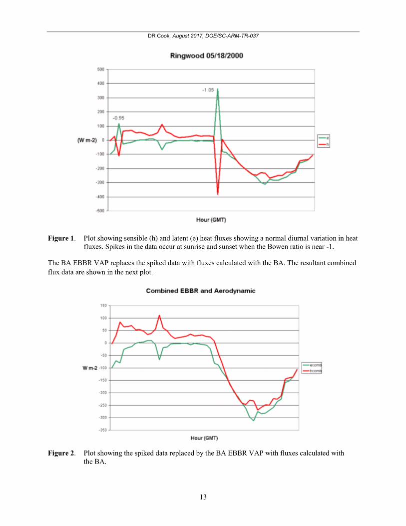
The following plot of sensible (h) and latent (e) heat fluxes show a normal diurnal variation in heat fluxes, with latent heat flux being mostly negative during nighttime hours, as evaporation continues, and sensible heat flux being positive. During daylight hours, both h and e are negative, as energy is lost from the surface. The plot also shows the spikes in the data that can occur at sunrise and sunset when the Bowen ratio is near -1 (see the Bowen ratios annotated on the plot, near the data spikes).


13

Figure 1. Plot showing sensible (h) and latent (e) heat fluxes showing a normal diurnal variation in heat

fluxes. Spikes in the data occur at sunrise and sunset when the Bowen ratio is near -1.

The BA EBBR VAP replaces the spiked data with fluxes calculated with the BA. The resultant combined flux data are shown in the next plot.

Figure 2. Plot showing the spiked data replaced by the BA EBBR VAP with fluxes calculated with

the BA.


14

5.3 User Notes and Known Problems

Some conditions do not require Data Quality Reports (DQRs) because they occur somewhat frequently. These conditions include spikes in the sensible and latent heat fluxes when the Bowen ratio is near -1, short periods when the automatic exchange mechanism (AEM) is not functioning properly (this can be detected from the quality control [QC] checks in the data files), and short periods of missing data.

Common instrumentation problems include:

• condensation or frost on the net radiometer upper polyethylene dome (this can persist well into daylight hours)

• net radiometer desiccant degradation

• holes in the net radiometer top dome caused by bird claws (this can result in water in the net radiometer if the dome is not replaced before precipitation occurs)

• soil sensors pulled from the ground or chewed by animals

• a blown fuse in the AEM when the belt slides bind against the track

• seized bearings in wind instruments

• aging of sensors and electronic components

• loosened electronic connections.

Preventative maintenance visits every two weeks and instrument mentor quality assurance activities are designed to detect and correct these problems to reduce the amount of incorrect data collected.

5.4 Frequently Asked Questions

How is the latent heat flux and sensible heat flux derived?

The Bowen ratio technique is used to determine Bowen ratio, assuming that the transfer coefficients of heat and water vapor are the same. The Bowen ratio is then used in conjunction with net radiation and soil surface heat flux measurements to determine sensible and latent heat flux based on a budget approach. More details are provided in Section 7.2, Theory of Operation.

What is the sign convention used for the energy flux densities?

All energy flux densities have a positive sign when directed toward the surface, and negative when directed away. For example, values of sensible (h) and latent heat flux (e) could be 0 to -600 watts per meter squared during the daytime in the summer.

In the design of the EBBR stations, which data are considered the most useful to Atmospheric Radiation Measurement (ARM) Science Team members?

The EBBR stations were designed primarily for computation of the sensible and latent heat fluxes. The soil temperature, moisture, and heat fluxes are measured in the upper 5 cm of the soil and therefore are not very useful for determining root zone soil moisture and soil heat flow. Other observations, such as air


15

temperature, RH, atmospheric pressure, and wind speed and direction are secondary measurements; Surface Meteorological Instrumentation (MET) measurements, where available, should be used as the absolute measurements of these quantities. For example, the EBBR atmospheric pressure data are not measured with sufficient accuracy for many applications, whereas the MET pressure data have a smaller uncertainty and might be suitable for calculations of geostrophic winds. Other sources of reliable surface meteorological data are available as external data for the ARM Facility from the Oklahoma Mesonet and from the Kansas network. The data user is encouraged to use the data from the MET for such observations.

EBBR data are collected only at the ARM Southern Great Plains (SGP) extended facilities, including one at the Central Facility (CF) and some that are collocated with boundary facilities, and where the local surface is not tilled. Eddy correlation stations exist at nearly half of the extended facilities to sample the latent heat, sensible heat, and momentum fluxes above tilled cropland.

EBBR data can be used to compute momentum fluxes with a bulk aerodynamic approach. This approach is used as the basis for the calculation of sensible and latent heat fluxes by the BA EBBR VAP (Wesely et al. 1995).

What do AEM home signals indicate?

The AEM home signal outputs in the 5-, 15-, and 30-minute datastreams are in units of millivolts DC. The circuitry producing the millivolt output is fairly rudimentary, and therefore the millivolt value is proportional to the DC voltage output of the EBBR power supply (solar/AC charged battery). The home signal can therefore vary significantly diurnally and can fall to unacceptable levels for the 15-minute value if battery performance degrades too much.

During the first and third quarter hours, the right side (looking from behind the AEM) aspirated radiation shield (housing temperature and RH probes) is normally in the “bottom” (lowest elevation) position, and the left side is in the “top” (greatest elevation) position. During this AEM state, the 5-minute “home,” 15-minute “mv_home”, and 30-minute “home_15” values should be between 40 and 55.

During the second and fourth quarter hours, the left side (looking from behind the AEM) aspirated radiation shield (housing temperature and RH probes) is normally in the “bottom” (lowest elevation) position, and the right side is in the “top” (greatest elevation) position. During this AEM state, the 5-minute “home,” 15-minute “mv_home,” and 30-minute “home_30” values should be between 15 and 30.

What soil measurements are made by the EBBR stations?

Five soil heat flow sensors are located at a depth of 5 cm below the surface, five long platinum resistance temperature detectors (PRTDs) integrate the temperature from the surface to a depth of 5 cm, and five soil moisture probes are located at a depth of 2.5 cm. Each set of five soil sensors is averaged. Because soil is not horizontally homogeneous, the sensors are spaced out in the soil locally to provide representative samples.

The purpose of these sensors is to compute one term, the surface soil heat flux. The soil temperature and moisture probes allow calculation of energy storage in the layer of soil between the surface and the heat


16

flow plate depth of 5 cm. The soil moisture probes allow the soil heat flow measurements to be adjusted for the conductivity of the soil.

The sensible and latent heat fluxes are computed by the EBBR data logger with the standard energy balance equation, in which the surface soil heat flux is usually a relatively small term. The surface soil heat flux term cannot be precisely recalculated from the raw information because of the way the soil energy storage term is computed with the EBBR data logger, but, in principle, the raw information can be used to recompute the sensible and latent heat fluxes with only a few percent error.

If some of the soil probes are not working, can sensible and latent heat fluxes be recalculated?

Yes. The remaining working soil probe sets can be used to calculate an average surface soil heat flux. See the procedure in Section 7.2, Theory of Operation.

What type of diurnal trends should appear in the EBBR data?

Some examples of diurnal trends can be seen in various textbooks and articles. For example, some data are shown in the special First ISLSCP Field Experiment (FIFE) issue of the Journal of Geophysical

Research (97: 18,343–19,110), e.g., the article by Fritschen et al. beginning on p. 18,697. The ARM Facility uses a Fritschen-type EBBR station.

What can be said about the quality of the EBBR data?

The EBBR systems sometimes experience hardware problems. For example, the AEM will sometimes malfunction. Some problems, like this one, can be discerned by looking at the data quality flags.

The following information should be useful for interpretation of the quality of data from the EBBR stations. Data quality flags should be used to detect when the AEM is functioning properly. The rate of AEM failure has been high at times. When it is not working, the estimates of sensible and latent heat flux are unreliable and should not be used for any scientific investigations, even if the flux estimates appear to be reasonable.

To use the metadata on the AEM, the user should become familiar with the field and global attributes described in a dump of the netCDF header. The fields are defined there, and, in data sets recently provided, the configuration of the data quality flags is briefly described at the end of the list of the global attributes. The flags themselves are contained in numbers at the end of the data listing. The next paragraph provides some suggestions on the QC numbers (qcmin# and qcmax#) and the embedded flags relevant to the AEM.

QC flags in the standard 30-minute data interval indicate when the AEM is working for each half hour in the time series. The particular QC flags of interest are the sixth and seventh bits of the 24-bit binary numbers representing qcmin49-72 and qcmax49-72. The sixth bit of qcmin49-72 is set to zero when the home_15 is greater than 35 mV, and to unity when less. The sixth bit of qcmax49-72 is set to zero when the home_15 is less than 70, and to unity when greater. A similar set of criteria are applied to the seventh bit, but with a minimum of 15 and maximum of 34.999999. Alternatively, if you choose not to convert the QC numbers to binary form, you can inspect the values of home_15 and home_30 to determine if they fall in the desired range. Because the limit checks on the home signals were not properly set prior to


17

April 7, 1993, you must inspect home_15 and home_30, rather than qcmin# and qcmax# for data collected prior to that date.

The QC flags should routinely be used for all of the variables. For some variables, however, QC flags have not been set, and for some variables (e.g., average soil heat flux [ave_shf], latent heat flux [e], and sensible heat flux [h]), flags were not set until late May 1998, as is evident in the listing of the field attributes. Nevertheless, some information can be obtained by inspection of the data if you are familiar with typical values. For example, Bowen ratios tend to be positive during the day and negative at night. Daytime values are usually between 0 and 2, and nighttime values can vary widely between positive values and -50. A negative Bowen ratio during daylight hours should be considered as possibly indicating suspect sensible and/or latent heat flux values. During transition times lasting up to two half hours near sunrise and sunset, the magnitude of the Bowen ratio can sometimes be quite large, in which case the sensible and latent heat flux values should be viewed as suspect. Although no QC flags were set for latent and sensible heat flux, values smaller than -1000 watts per meter squared and larger than 200 watts per meter squared are clearly suspect.

Routine checks reveal an expected offset drift of the RH probe of about +2% per year caused by aging and dirt contamination of the RH sensing element. This drift has also been observed in the Tower and MET RH probes. Although this affects the absolute accuracy of the RH measurement, it does not adversely affect the 30-minute vapor pressure difference calculated from the RH and temperature measurements because the RH probes drift at approximately the same rate, and the AEM exchanging Bowen ratio technique reduces offset effects. Recalibration after two years of use is usually recommended to keep the RH probes within their “as new” absolute accuracy specification; this is the goal of the EBBR recalibration program conducted every two years.

The absolute value of the home signals varies with the voltage of the battery that powers the EBBR data acquisition system. When the battery condition is good, the home_15 value is typically between 40 and 55; the home_30 value is typically between 15 and 30. When battery condition is low, the home signals can be slightly lower, but then the data from some individual sensors are questionable. Instances have occurred where low battery condition allowed some sensors to function while others did not. DQRs are written to identify such problems.

Unfortunately, the AEM does not always switch and occasionally hangs up. Four cases are common:

1. AEM fuse blown. When the fuse blows, the housing positions on the AEM are uncertain and usually yield home_15 and/or home_30 values of zero, although E15 at Ringwood, Oklahoma, showed -2.0 in this condition in May 1994. Usually the fuse blows because of too much friction on the exchange mechanism resulting from freezing rain or snow, built-up dirt, or an electrical or electronic failure.

2. AEM stuck at one position. Usually the right housing will stick in the down position (sometimes referred to in site operations log messages as the home position). When this happens, the home_15 and home_30 signal outputs are usually both equal to the proper home_30 value, if the AEM fuse has not blown. There are exceptions to this, of course, which included a period at the Central Facility EBBR in late 1992 when both home signals were 35.

3. AEM stuck between the 15- and 30-minute positions. This situation usually produces a very small negative home value for both home_15 and home_30, such as -0.2.


18

4. AEM removed for service. Occasionally, an AEM has been removed from service for repair when no replacements were available (e.g., when the EBBR at E9, Ashton, Kansas, was removed on April 5, 1994). A resistor in the AEM circuitry had burned out, leaving the left housing in the bottom position (a rarity). This had resulted in both home signals showing somewhere from 67 to 73. After the AEM was removed, the aspirated housings were tied to the EBBR frame, approximately a meter apart. Without the AEM circuitry being present, the home signals floated to the thousands. On April 19, a refurbished AEM was installed and the home signals returned to normal.

The list above illustrates only some of the possibilities. Generally, whatever their absolute values, if the home_15 and home_30 values are practically the same in the 30-minute data, at least one of them is incorrect, indicating that the sensible and latent heat flux estimates are suspect. Unless both the home_15 and home_30 values are within proper ranges, the sensible and latent heat values must be considered incorrect. No other interpretation is appropriate. Even if we know the AEM position situation and could thus recalculate fluxes from the available data, those fluxes would still be corrupted with calibration offsets, which are normally removed via the AEM switching process.

Most users of the EBBR data only receive the 30-minute data and not the 5- or 15-minute data. The QC flags in the 15-minute data might be useful for a comprehensive evaluation of each EBBR sensor. For example, the qcmin# check for battery condition in the 15-minute data is set to the lowest value at which the sensors will typically operate reliably. Also, soil moisture resistance ratios (rr_sm#, used before April 1996) or soil moisture resistance (r_sm#, used beginning in April 1996) could be examined to help determine when individual soil moisture values are reliable. However, we do not expect every user of the EBBR to obtain the 15-minute data for such analyses. Finally, users of the data are cautioned that the reliability and accuracy of some individual sensors, such as soil moisture sensors, may be not optimal.

The EBBR system was not designed to observe all quantities extremely well because its primary purpose is to provide sensible and latent heat flux estimates, which are not particularly sensitive to the uncertainties of some of the variables. For example, if accurate, reliable estimates of barometric pressure and air temperature are needed, the values supplied by MET or from external data sets, such as those from the Oklahoma Mesonet, should be used. For soil moisture and temperature, we consider the EBBR observations to be mostly inadequate for use in land-surface process and hydrological models or submodels. On the other hand, we expect high-quality data on net radiation from EBBR stations because it is crucial in the energy balance calculations. We expect soil heat flux values to be good because they enter directly into the surface energy balance calculations (but are typically small in magnitude compared to net radiation). Unforeseen types of failures sometimes occur, e.g., the ventilator for one of the temperature and humidity sensors stops. Such problems are usually described in DQRs that are available for data users.

When the Bowen ratio is between -1.6 and -0.45, “spikes” can occur in the latent and sensible heat flux values.

What are likely difficulties in comparing surface heat fluxes measured by EBBR stations to results of numerical modeling efforts?

One of the greatest difficulties in comparing model versus field data on surface heat fluxes is caused by model calculations requiring soil moisture information. The soil moisture across the SGP site can be quite variable for summertime conditions. EBBR soil moisture data provide measurements of average moisture


19

content only in the top 5 cm. During 1996 and 1997, an effort led by Jeanne Schneider, University of Oklahoma, and supported by the National Oceanic and Atmospheric Administration for GEWEX Continental-Scale International Project (GCIP), installed soil water and temperature system (SWATS) profiling instrumentation at every SGP extended facility, including every location with an EBBR station. SWATS soil moisture and soil temperature data should be used for modeling efforts, instead of the EBBR soil moisture and temperature data.

Since summer 1995, at least three science team groups have tried comparing model outputs with SGP site data: Jim Liljegren working with Chris Doran at Pacific Northwest Laboratory; Marina Zivkovic working with Jean-Francois Louis at Atmos. & Environmental Research, Inc., in Cambridge, Massachusetts; and Sarah Fox working with Lee Harrison and others at the State University of New York at Albany.

A cooperative program of sorts that has looked extensively at this type of modeling is the Project for Intercomparison of Land-surface Schemes (PILPS). One conclusion of PILPS is that more observational data are needed for developing large-scale models. For example, an article by Betts et al. (1993) carries out a critical evaluation of European Center for Medium Range Weather Forecasts (ECMWF) model outputs by using FIFE data.

Some other potentially informative articles are as follows:

Avissar, R, and MM Verstraete. 1990. “The representation of continental surface processes in atmospheric models.” Reviews of Geophysics 28(1): 35–42, doi:10.1029/RG028i001p00035.

Dickinson, RE, RM Errico, F Giorgi, and GT Bates. 1989. “A regional climate model for the Western United States.” Climatic Change 15(3): 383–422, doi:10.1007/BF00240465.

Shuttleworth, WJ. 1991. “Insight from large-scale observational studies of land/atmosphere interactions.” Surveys in Geophysics, 12(1-3): 3–30, doi:10.1007/BF01903410.

6.0 Data Quality

6.1 Data Quality Health and Status

The status of the measurements made by the EBBR system can be found by going to the ARM DQ Explorer web page at http://dq.arm.gov/dq-explorer/cgi-bin/main/metrics.

6.2 Data Reviews by Instrument Mentor

Monthly reviews of the EBBR data were prepared by the mentor and submitted to the Instrument Mentor Monthly Summary (IMMS) report database until these ended in late 2014.

Beginning in FY2006, Data Quality Reports are not written for missing data of less than a day in length or for situations when QC flags clearly show that the data are incorrect (this is true for most of the conditions listed below). DQRs are written for periods when data are incorrect, when the situation is not represented by QC flags in the data, and it is not obvious that the data should have been flagged as incorrect.

http://onlinelibrary.wiley.com/doi/10.1029/RG028i001p00035/full

https://link.springer.com/article/10.1007/BF00240465



20

6.3 Data Assessments by Site Scientist/Data Quality Office

The following guidance has been provided by the EBBR mentor for use by the Data Quality Office (DQO) in preparing their weekly assessment report for the EBBR systems.

EBBR Data Quality Guidance

David R. Cook 16 December, 2006

Introduction: The best way to tell someone what to look for in assessing the EBBR data is to describe conditions that reflect correct and incorrect data. For the most part, the QC checks provide adequate guidance. However, there are conditions for which the QC flags do not provide the needed guidance to be able to interpret the correctness of the data. Therefore, please use the information below as further guidance.

Primary Measurements: e (latent heat flux), h (sensible heat flux), q (net radiation), ave_shf (average surface soil heat flux); le and h are calculated, whereas q and ave_shf are measured. The QC limits set in the ingest are appropriate for the measurements (primary and otherwise), although at times legitimate values fall outside the QC limits.

Nuisance QC Flags: The Bowen QC flag is frequently tripped, particularly at sunrise or sunset, when the gradient of temperature can be near zero. This condition produces spikes in h and e, which would be quite obvious without the Bowen QC flag. Tripping of the Bowen QC flag near sunrise or sunset should not be reported in the DQO assessment reports. The hum_top and hum_bot QC flags will trip when the RH reported by the T/RH sensor exceeds a certain value. However, the absolute accuracy of the RH measurements is not important; the difference between them is used to determine e. Therefore, the hum_top and hum_bot QC flag condition should not be reported in the DQO assessment reports.

Comparison of Data at Different EBBR Sites: Generally, the measurements can be compared favorably with those at adjacent sites, keeping in mind that climate conditions from one side of the SGP facility to another can differ sharply. There are some soil and surface vegetation differences between sites as well, so comparisons may show significant differences.

Comparison of Data with the Eddy Correlation System (ECOR): The only collocated ECOR and EBBR are at the SGP Central Facility (CF) and at EF39, Morrison, OK. Caution must be used in the comparison of the two systems at SGP CF because they may see different vegetation surfaces (Cook et al. 2006). At the CF the best comparison can be made for straight north or northwest wind directions, when both systems view the same grass surface. For other directions, the two systems are viewing different vegetation surfaces and the fluxes from the two will probably not be similar, unless perhaps the ground is snow covered. At EF39 the EBBR and ECOR see the same surface, whether the wind blows over the wheat or the grass. Sensible and latent heat flux, and wind speed and direction measurements, could be compared for adjacent ECOR and EBBR sites, again remembering that climatologically driven differences are likely.

Comparison of Data with the MET: MET systems are collocated with EBBR systems at 8 of the 14 EBBR sites (exceptions are E2, E12, E18, E19, E22, and E26). The measurements of upper EBBR


21

temperature, RH, and vapor pressure can be directly compared with the MET temperature, RH, and vapor pressure. Even so, the EBBR RH may often be greater than that from the MET, as it is allowed to drift upwards with time for longer than is allowed for the MET. Wind speed and direction for the two systems are at different heights (MET 10 m, EBBR ~3 m), so it is normally expected that the MET wind speed will be greater than the EBBR wind speed. Wind direction may be very similar, but may be somewhat different if a frontal passage or strong advection is taking place. The EBBR pressure measurement is not as accurate as that made by the MET, but their trends and general level may be compared in a gross way.

Comparison of EBBR Net Radiation with Solar and Infrared Station (SIRS) Net Radiation: EBBR net radiation measurements do not agree with SIRS net radiation calculations when the effective sky temperature is less than about -20 °C and the EBBR net radiometer sensitivity decreases rapidly with the further decrease in effective sky temperature. First, the REBS longwave calibration is not performed to very low temperatures, and second, the design of the net radiometer may not allow for accurate low effective sky temperature measurements. Infrared thermometer (IRT), atmospheric emitted radiance interferometer (AERI), and SIRS net radiation measurements are more accurate under the condition of low effective sky temperatures.

The result of this situation is that the EBBR overestimates or underestimates (it sounds odd, but it can be either) the nighttime sensible heat flux (direction is to the surface) and overestimates (sometimes by possibly a factor of 3) the nighttime latent heat flux. This is not a major concern since the nighttime fluxes are usually quite small anyway. Daytime fluxes are also affected, but since shortwave radiation dominates the radiant energy budget, the sensible and latent heat fluxes are both overestimated by only about 5 percent during a sunny day and by about 2 percent on a cloudy day during summertime. These errors are well within the 10 percent system error of the EBBR.

Common Conditions Reflecting Correct or Incorrect Data:

The EBBR data are only useful for particular wind directions at each extended facility. Please use the following resources to help in interpreting the EBBR data:

1. QC flags in the EBBR data.

2. IMMS at http://www.db.arm.gov/IMMS/.

3. The information below on wind direction dependencies and conditions that commonly cause incorrect data.

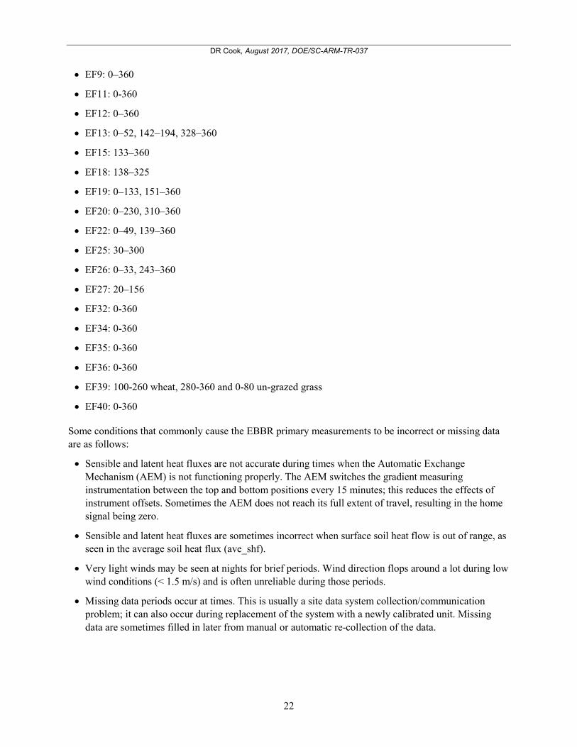
Wind Direction Dependencies (numbers are wind direction in degrees); note that there are wind directions at most sites for which the fetch is insufficient and therefore EBBR data are invalid. Appropriate fetch was determined from a 1/40 measurement height to fetch ratio, resulting in a required minimum fetch of 120 m. Particular attention should be paid to the limited valid wind directions for the Central Facility EBBR. The surface vegetation type for the EBBRs is grazed or ungrazed grassland (refer to the Extended Facility Surface Conditions Observations [EFSCO] for state):

• EF2: 71–137, 223–289

• EF4: 0–158, 202–360

• EF7: 0–244, 296–360

• EF8: 0–224, 314–360

http://www.db.arm.gov/IMMS/


22

• EF9: 0–360

• EF11: 0-360

• EF12: 0–360

• EF13: 0–52, 142–194, 328–360

• EF15: 133–360

• EF18: 138–325

• EF19: 0–133, 151–360

• EF20: 0–230, 310–360

• EF22: 0–49, 139–360

• EF25: 30–300

• EF26: 0–33, 243–360

• EF27: 20–156

• EF32: 0-360

• EF34: 0-360

• EF35: 0-360

• EF36: 0-360

• EF39: 100-260 wheat, 280-360 and 0-80 un-grazed grass

• EF40: 0-360

Some conditions that commonly cause the EBBR primary measurements to be incorrect or missing data are as follows:

• Sensible and latent heat fluxes are not accurate during times when the Automatic Exchange Mechanism (AEM) is not functioning properly. The AEM switches the gradient measuring instrumentation between the top and bottom positions every 15 minutes; this reduces the effects of instrument offsets. Sometimes the AEM does not reach its full extent of travel, resulting in the home signal being zero.

• Sensible and latent heat fluxes are sometimes incorrect when surface soil heat flow is out of range, as seen in the average soil heat flux (ave_shf).

• Very light winds may be seen at nights for brief periods. Wind direction flops around a lot during low wind conditions (< 1.5 m/s) and is often unreliable during those periods.

• Missing data periods occur at times. This is usually a site data system collection/communication problem; it can also occur during replacement of the system with a newly calibrated unit. Missing data are sometimes filled in later from manual or automatic re-collection of the data.


23

6.4 VAPS and Quality Measurement Experiments (QMEs)

The BA EBBR VAP represents a recalculation of sensible and latent heat fluxes using wind speed and temperature gradient information in conjunction with a bulk aerodynamic estimation technique. This VAP has been implemented, and 30-minute average files are available in the ARM Data Archive from 1995. Vegetation height and wind speed are used to determine aerodynamic quantities that allow the calculation of sensible and latent heat flux independent from measurements of net radiation and soil surface heat flux. These calculations help to produce more reasonable flux estimates when the Bowen ratio is between -1.6 and -0.45 (the Bowen ratio technique often produces unreasonable flux values under this condition). Data source names take the form “sgp30baebbrE13.c1.” Presently, the files can be found in the ARM Data Archive by looking under c1 data sources. Results from the BA EBBR VAP can be seen in the second plot in Section 5.2, Annotated Examples.

A second VAP involves the recalculation of sensible and latent heat fluxes using Solar and Infrared Station (SIRS) net radiation information; however, this VAP has not been implemented. This approach may help to improve flux estimates during times when the EBBR net radiation data are corrupted by dew, frost, or condensation inside or outside of the net radiometer domes.

EBBR-related QMEs could include:

• Comparison of EBBR-measured net radiation and SIRS-calculated net radiation. Comparison plots of EBBR net radiation and SIRS-calculated net radiation are produced by the DQO and displayed on the DQ Explorer website. These comparison plots reveal significant differences between these two systems at times. A QME has not yet been performed.

• Comparison of sensible and latent heat fluxes from EBBR and ECOR systems can only be made at the SGP Central Facility (only for very limited wind directions; within 30 degrees east or west of north) and at EF39.

7.0 Instrument Details

7.1.1 List of Components

• Vaisala T/RH probes at two heights (1-m separation), in aspirators

• PRTD temperature probes at two heights (1-m separation), in aspirators

• REBS Q*7.1 Net Radiometer (at 2 m typical)

• REBS SMP-2 (5 sets) Soil Moisture Probes at 2.5 cm depth

• REBS HFT-3 (5 sets) Soil Heat Flow Plates at 5 cm depth

• REBS STP-1 (5 sets) Soil Temperature Probes, integrated 0 to 5 cm

• Met One Instruments 090C or 090D Barometric Pressure sensor (in enclosure)

• Met One 020C Wind Direction sensor at 2.5 m

• Met One 010C Wind Speed sensor at 2.5 m


24

• PRTD Reference temperature of control box

• REBS AEM

• Pipe network structure for mounting of the instrumentation

• Solar panel, battery, AC charger power source

• Enclosure holding Campbell CR10, multiplexers, J-panels, communication equipment.

7.1.2 System Configuration and Measurement Methods

The EBBR sensors (except for soil probes) are mounted on a triangular pipe framework that sits on the soil surface. The net radiometer mount extends from the south end of the EBBR frame.

A unique aspect of the system is the AEM, which helps to reduce errors from instrument-offset drift. The AEM extends from the north end of the frame. Aspirated radiation shields (which house the air temperature and temperature/RH probes) are attached to the AEM. The openings of the aspirated radiation shields face north to reduce radiation error from direct sunlight.

The soil probes are buried just outside the view of and in an arc to the south of the net radiometer.

The heights of the AEM aspirators are different at different extended facilities and depend on maximum vegetation height; the vertical separation between the two aspirators is 1 m at all extended facilities. The heights or depths of all other sensors are the same at all facilities.

The reference temperature sensor, barometric pressure sensor, data logger equipment, and communication equipment are located in a control box (weatherproof enclosure) attached at the northeast corner of the EBBR frame.

The local area of influence upon Bowen ratio measurements is contained within a horizontal distance of approximately 20 times the height of the top aspirated radiation shield on the AEM. This distance varies among the different extended facilities and for different times of the year because of differences in maximum vegetation height, and therefore the height at which the AEM is installed.

The manufacturer’s (REBS) name for these systems is SEBS (Surface Energy Balance System); this name appears in the systems documentation.

7.1.3 Specifications

The accuracies cited below are generally those stated by the manufacturer. They are sensor-absolute accuracies and do not include the effects of system (i.e., data logger) accuracies. Although it is not known how some of the manufacturers have determined sensor accuracy, it is properly the root square sum of any nonlinearity, hysteresis, and non-repeatability, usually referenced as percentage of full scale.

The detection limit is normally restricted to the range (sometimes called Calibrated Operating Range) over which the accuracy applies. In the case of the EBBR, some of the detection limits are those determined by the vendor (REBS) who performed the calibration, not by the manufacturer of the sensor. Some manufacturers also specify an Operating Temperature Range in which the sensor will function both


25

physically and electronically, even though the calibration may not be appropriate for use throughout that range. When the manufacturer or the calibrating vendor has listed no detection limits, none are stated below.

Air temperatures: Chromel-constantan thermocouple, Omega Engineering Inc., REBS Model # ATP-1, Detection Limits -30 to 40°C, Accuracy +/- 0.5°C.

Temperature/RH Probe: Operating Temperature Range -20 to 60°C. Temperature: Platinum Resistance Temperature Detector (PRTD); Detection Limits -30 to 40°C, Accuracy +/- 0.2°C RH: Capacitive element, Vaisala Inc., Model #s HMP 35A and HMP 35D; Detection Limits 0% to 100% RH, Accuracy +/- 2% (0-90% RH), +/- 3% (90-100%), uncertainty of RH calibration +/- 1.2%.

Soil Temperature: Platinum Resistance Temperature Detector, MINCO Products, Inc., REBS Model # STP-1, MINCO Model # XS11PA40T260X36(D), Detection Limits -30 to 40°C, Accuracy +/- 0.5°C.

Soil Moisture: Soil Moisture Probe (fiberglass and stainless steel screen mesh sandwich), Soiltest, Inc., REBS Model # SMP-2, Soiltest Model # MC-300, Accuracy not specified by manufacturer (varies significantly depending on soil moisture and soil type). Detection limits for this sensor are limited by the ability to fit a polynomial to the calibration data; for the SGP site, the detection limits are approximately 1% to 50% by volume.

Soil Heat Flow: Soil Heat Flow Probes, Radiation & Energy Balance Systems, Inc., Model #s HFT-3, HFT3.1, Accuracy not specified by manufacturer.

Barometric Pressure: Barometric Pressure Sensor, Met One Instruments, Model #s 090C-24/30-1, Detection Limits 24 to 30 kPa; 090C-26/32-1, Detection Limits 26 to 32 kPa; 090D-26/32-1, Detection Limits 26 to 32 kPa; Accuracy for all +/- 0.14 kPa.

Net Radiation: Net Radiometer, Radiation & Energy Balance Systems, Inc., Model Q*6.1 or Q*7.1, Accuracy +/- 5% of full-scale reading.

Wind Direction: Wind Direction Sensor, Met One Instruments, Model #s 5470, 020C, Detection Limits 0 to 360° physical (for greater than 0.3 ms-1 wind speed), 0 to 356° electrical, Accuracy +/- 3°.

Wind Speed: Wind Speed Sensor, Met One Instruments, model #s 010B and 010C, Operating Temperature Range -50 to 85°C, Detection Limits 0.27 to 50 ms-1, Accuracy +/- 1% of reading. Operational Limit on speed 60 ms-1.

Data logger: Campbell Scientific, Inc., Model CR10, Detection Limits vary by voltage range selected, Accuracy +/- 0.1% of full scale reading.

7.2 Theory of Operation

The EBBR stations use a standard Bowen ratio approach that has been described by textbooks and articles. A general description can be found in Brutsaert (1982). For an article, see p. 18,549 of the special FIFE issue of the Journal of Geophysical Research (97): 18,343–19,110).


26

The surface energy balance equation is used:

q + ave-shf + h + e = 0,

where q is net radiation, ave_shf is the ground surface heat flow, h is sensible heat flux, and e is latent heat flux. The units for the terms in the equation above are watts per meter squared.

ave_shf is measured with five sets of soil heat flow, soil temperature, and soil moisture probes. Soil heat flow at 5 cm (shf1, shf2, shf3, shf4, shf5), measured with soil heat flow plates, and soil energy storage (ces1, ces2, ces3, ces4, ces5) in the 0–5 cm layer (measured as the change in temperature with time) are added to obtain surface soil heat flow, as follows:

g1 = shf1 + ces1,

etc.,

where shf1 and ces1 are, respectively, the soil heat flow from the soil heat flow plate and the change in energy storage measured from the soil temperature probe of soil set #1. The expressions for g2, g3, g4, and g5 are similar. Soil moisture is used to adjust the measurements for soil thermal conductivity, which affects the calibrations of the sensors.

Surface soil heat flow is then

ave_shf = (g1 + g2 + g3 + g4 + g5)/5,

When data from one or more soil set(s) is incorrect, that soil set(s) can be eliminated and the average soil heat flow determined from the remaining sets.

The Bowen ratio is measured as the ratio of the gradients of temperature and vapor pressure (the latter calculated from RH and temperature) across two fixed heights within three meters of the surface.

The Bowen ratio (B = h/e) is computed on the basis of the gradients and the following computations are performed:

e = -(q + ave_shf)/(1 + B)

h = B * e

More detailed information on these and other equations can be obtained elsewhere, including from David Cook at Argonne National Laboratory. A large manual provided by the manufacturer, REBS, Inc., describes the general theory, gives rather complete information on each type of sensor, and explains procedures for installation, operation, and maintenance.


27

7.3 Calibration

7.3.1 Theory

Standard calibration procedures are employed by the vendor(s) of the sensors and equipment used in the EBBR system when each EBBR unit is returned for recalibration, approximately every two years.

7.3.2 Procedures

Net Radiometer: Calibration is performed in a temperature-controlled, black-body cavity chamber against a transfer standard. The light source is a tungsten-halide lamp. The transfer standard was calibrated both in the temperature-controlled cavity chamber and by comparison to an Eppley precision pyranometer outdoors. Wind speed effects are also taken into consideration by ventilating the radiometers in the calibration chamber and outdoors. The transfer standard is traceable to the National Institute of Standards and Technology (NIST) through the Eppley pyranometer using a shading technique. Shortwave and longwave calibrations are different, and so they are applied appropriately for daytime and nighttime conditions in the EBBR programming. The longwave calibration performed by REBS does not provide correct measurements under conditions of low effective sky temperatures (below about -30°C).

7.3.3 History

The EBBR systems are returned to REBS approximately every two years for calibration of all sensors and data logger equipment. Some of the calibrations are performed by REBS themselves, while some are performed by manufacturers of the equipment. For various reasons (the need to provide and calibrate spare sensors, frequent AEM failures, etc.) the time between recalibrations of EBBR units has sometimes been greater than two years; REBS is a small company and has little flexibility to reprioritize rapidly for individual customers.

7.4 Operation and Maintenance

7.4.1 User Manual

A user manual is available from REBS for the SEBS systems. One copy is kept at the SGP Central Facility, and the mentor keeps one copy.

7.4.2 Routine and Corrective Maintenance Documentation

SGP Site Operations (Site Ops) personnel maintain preventative maintenance, corrective maintenance, and engineering logs. Maintenance and system checks are performed in accordance with a set of procedures written by Site Ops and the mentor. These procedures are maintained in print form at the SGP Central Facility and in digital form on Site Ops laptops taken into the field during preventative maintenance visits to the EBBR systems.


28

7.4.3 Software Documentation

EBBR programs are maintained on SGP Site Ops computers at the SGP Central Facility, on laptops used by Site Ops during preventative maintenance visits, and at REBS. The mentor maintains print copies and some digital copies.

7.4.4 Additional Documentation

Six-month EBBR checks are maintained on the SGP Operations Management Information System (OMIS) website.

7.5 Glossary

Bowen Ratio: the ratio of the sensible heat flux to the latent heat flux.

Latent Heat Flux: the transfer of latent heat (heat released or absorbed by water) between the surface and the air, or vice versa.

Net Radiation: the net difference in downwelling and upwelling solar plus terrestrial radiation.

Sensible Heat Flux: the transfer of sensible heat (enthalpy) between the surface and the air, or vice versa.

Soil Heat Flow: the transfer of sensible heat (enthalpy) in the soil, towards the surface or away from the surface.

8.0 Citable References Avissar, R, and MM Verstraete. 1990. “The representation of continental surface processes in atmospheric models.” Reviews of Geophysics 28(1): 35–42, doi:10.1029/RG028i001p00035.

Betts, AK, JH Ball, and ACM Beljaars. 1993. “Comparison between the land surface response of the ECMWF model and the FIFE-1987 data.” Quarterly Journal of the Royal Meteorological Society 119(513): 975–1001, doi:10.1002/qj.49711951307.

Brutsaert, WH. 1982. Evaporation in the Atmosphere. D. Reidel Publishing Company, Dordrecht, Holland, pp. 210–212.

Dickinson, RE, RM Errico, F Giorgi, and GT Bates. 1989. “A regional climate model for the Western United States.” Climatic Change 15(3): 383–422, doi:10.1007/BF00240465.

Fritschen, LJ and LW Gay. 1979. Environmental Instrumentation. Springer-Verlag, New York, p. 216.

Fritschen LJ, P Qian, ET Kanemasu, D Nie, EA Smith, JB Steward, SB Verma, and ML Wesely. 1992. “Comparisons of surface flux measurement systems used in FIFE 1989.” Journal of Geographical

Research 97(D17): 18,697–18,713, doi:10.1029/9JD03042.

http://onlinelibrary.wiley.com/doi/10.1029/RG028i001p00035/full

http://onlinelibrary.wiley.com/doi/10.1002/qj.49711951307/abstract


http://onlinelibrary.wiley.com/doi/10.1029/91JD03042/abstract


29

Shuttleworth, WJ. 1991. “Insight from large-scale observational studies of land/atmosphere interactions.” Surveys in Geophysics 12(1-3): 3–30, doi:10.1007/BF01903410.

Wesely, MW, DR Cook, and RL Coulter. 1995. “Surface Heat Flux Data from Energy Balance Bowen Ratio Systems.” Preprints of the Ninth Symposium on Meteorological Observations and Instrumentation, pp. 486-489. Charlotte, North Carolina, March 27–31 1995, American Meteorological Society, Boston, Massachusetts. https://www.osti.gov/scitech/servlets/purl/69120

9.0 Bibliography Field, RT, L Fritschen, ET Kanemasu, EA Smith, J Stewart, S Verma, and W Kustas. 1992. “Calibration, comparison, and correction of net radiation instruments used during FIFE.” Journal of Geophysical

Research 97: 18681–18695, doi:10.1029/91JD03171.

Fritschen, L, and JR Simpson. 1989. “Surface energy and radiation balance systems: General description and improvements.” Journal of Applied Meteorology 28: 680–689, doi:10.1175/1520-0450(1989)028<0680:SEARBS>2.0.CO;2.

Halldin, S, and A Lindroth. 1992. “Errors in net radiometry: Comparison and evaluation of six radiometer designs.” Journal of Atmospheric Oceanic Technology 9: 762–783, doi:10.1175/1520-0426(1992)009<0762:EINRCA>2.0.CO;2.

Heilman, JL, and CL Brittin. 1989. “Fetch requirements for Bowen ratio measurements of latent and sensible heat fluxes.” Agricultural and Forest Meteorology 44(3-4): 261–273, doi:10.1016/0168-1923(89)90021-X.

Lewis, JM. 1995. “The story behind the Bowen ratio.” Bulletin of the American Meteorological Society 76: 2433–2443, doi:10.1175/1520-0477(1995)076<2433:TSBTBR>2.0.CO;2.


https://www.osti.gov/scitech/servlets/purl/69120

http://onlinelibrary.wiley.com/doi/10.1029/91JD03171/full

http://journals.ametsoc.org/doi/abs/10.1175/1520-0450%281989%29028%3C0680%3ASEARBS%3E2.0.CO%3B2

http://journals.ametsoc.org/doi/abs/10.1175/1520-0450%281989%29028%3C0680%3ASEARBS%3E2.0.CO%3B2

http://journals.ametsoc.org/doi/abs/10.1175/1520-0426%281992%29009%3C0762%3AEINRCA%3E2.0.CO%3B2

http://journals.ametsoc.org/doi/abs/10.1175/1520-0426%281992%29009%3C0762%3AEINRCA%3E2.0.CO%3B2

http://www.sciencedirect.com/science/article/pii/016819238990021X

http://www.sciencedirect.com/science/article/pii/016819238990021X

http://journals.ametsoc.org/doi/abs/10.1175/1520-0477(1995)076%3C2433%3ATSBTBR%3E2.0.CO%3B2

ebbr instrument handbook

Documents