earthquake simulation

8/8/2019 Earthquake Simulation

http://slidepdf.com/reader/full/earthquake-simulation 1/43

University Politehnica of Bucharest

Faculty of Automatic Control and Computers

Computer Science and Engineering Department

Diploma Thesis

Generation, simulation and

verification of the seismic

activity in the Vrancea region

by

Ioana Apetroaei

Supervisor: Associate Prof. Dr. Eng. Emil Slusanschi,

Bucharest, July 2010



Contents

Contents i

List of Figures iii

List of Tables v

1 Introduction 2

2 State of the Art and Related Work 4

2.1 Vrancea seismic activity . . . . . . . . . . . . . . . . . . . . . . . . 4

2.2 Seismic cycle features . . . . . . . . . . . . . . . . . . . . . . . . . 5

2.3 Burridge-Knopoff Model . . . . . . . . . . . . . . . . . . . . . . . . 72.4 Geodynamical model . . . . . . . . . . . . . . . . . . . . . . . . . . 8

2.4.1 Detachment Model . . . . . . . . . . . . . . . . . . . . . . . 9

2.4.2 Delamination Model . . . . . . . . . . . . . . . . . . . . . . 10

2.5 Starting point . . . . . . . . . . . . . . . . . . . . . . . . . . . . . . 11

2.5.1 Earthquake vizualization . . . . . . . . . . . . . . . . . . . 11

2.5.2 Earthquake simulation . . . . . . . . . . . . . . . . . . . . . 11

2.5.3 The duration of the simulated seismic cycles . . . . . . . . . 12

3 Project implementation 13

3.1 Hardware and Software Configuration . . . . . . . . . . . . . . . . 13

3.2 Simulation model . . . . . . . . . . . . . . . . . . . . . . . . . . . . 14

3.3 Cellular Automaton methods . . . . . . . . . . . . . . . . . . . . . 15

3.4 Simulation parameters . . . . . . . . . . . . . . . . . . . . . . . . . 15

3.4.1 The initialization of the grid . . . . . . . . . . . . . . . . . 17

3.4.2 Background events . . . . . . . . . . . . . . . . . . . . . . . 17

3.4.3 Asperity type events . . . . . . . . . . . . . . . . . . . . . . 17

3.4.4 Percolation type events . . . . . . . . . . . . . . . . . . . . 19

3.5 Healing process . . . . . . . . . . . . . . . . . . . . . . . . . . . . . 19

i



CONTENTS ii

4 Case studies 21

4.1 Gutenberg Richter Law . . . . . . . . . . . . . . . . . . . . . . . . 21

4.2 Real catalogue . . . . . . . . . . . . . . . . . . . . . . . . . . . . . 224.2.1 Initialization . . . . . . . . . . . . . . . . . . . . . . . . . . 22

4.2.2 Reinitialization . . . . . . . . . . . . . . . . . . . . . . . . . 23

4.2.3 Gutenberg-Richter law . . . . . . . . . . . . . . . . . . . . . 25

4.2.4 Magnitude-events order . . . . . . . . . . . . . . . . . . . . 26

4.2.5 Numerical results . . . . . . . . . . . . . . . . . . . . . . . . 27

4.3 1000 trials . . . . . . . . . . . . . . . . . . . . . . . . . . . . . . . . 28

4.3.1 Initialization . . . . . . . . . . . . . . . . . . . . . . . . . . 28

4.3.2 Gutenberg-Richter law . . . . . . . . . . . . . . . . . . . . . 29

4.3.3 Magnitude-events order . . . . . . . . . . . . . . . . . . . . 30

4.3.4 Numerical results . . . . . . . . . . . . . . . . . . . . . . . . 31

5 Conclusions 33

6 Future work 35

Bibliography 36



List of Figures

2.1 Successive cumulative processes in Vrancea as revealed by Benioffs curves. 72.2 Burridge-Knopoff Model. . . . . . . . . . . . . . . . . . . . . . . . . . 8

2.3 Detachment model. . . . . . . . . . . . . . . . . . . . . . . . . . . . . . 9

2.4 Delamination model. . . . . . . . . . . . . . . . . . . . . . . . . . . . . 10

2.5 The duration of 10000 simulated seismic cycles. . . . . . . . . . . . . . 12

3.1 Neighbourhood types. . . . . . . . . . . . . . . . . . . . . . . . . . . . 15

3.2 The black cells influenced by the introduction of an gray cell. . . . . . 18

4.1 The cells from the real catalogue of earthquakes. . . . . . . . . . . . . 22

4.2 The grid in the moment the initialization is finished. . . . . . . . . . . 23

4.3 The clusters that were not destroyed in the previous seismic cycle. . . 23

4.4 The grid after the insertion of the earthquakes epicenter. . . . . . . . . 24

4.5 The grid after the reinitialization for a new seismic cycle. . . . . . . . 24

4.6 Gutenberg-Richter law for the first seismic cycle. . . . . . . . . . . . . 25

4.7 Gutenberg-Richter law for the second seismic cycle. . . . . . . . . . . . 25

4.8 Gutenberg-Richter law for the third seismic cycle. . . . . . . . . . . . 25

4.9 Gutenberg-Richter law for the fourth seismic cycle. . . . . . . . . . . . 25

4.10 Magnitudes-events order for the first seismic cycle. . . . . . . . . . . . 26

4.11 Magnitudes-events order for the second seismic cycle. . . . . . . . . . 26

4.12 Magnitudes-events order for the third seismic cycle. . . . . . . . . . . 26

4.13 Magnitudes-events order for the fourth seismic cycle. . . . . . . . . . . 26

4.14 Simulated catalogue. . . . . . . . . . . . . . . . . . . . . . . . . . . . . 27

4.15 The cells randomly inserted-1000 trials. . . . . . . . . . . . . . . . . . 28

4.16 The grid in the moment the initialization is finished-1000 trials. . . . . 29

4.17 Gutenberg-Richter law for the first seismic cycle. . . . . . . . . . . . . 29

4.18 Gutenberg-Richter law for the second seismic cycle. . . . . . . . . . . . 29

4.19 Gutenberg-Richter law for the third seismic cycle. . . . . . . . . . . . 30

4.20 Gutenberg-Richter law for the fourth seismic cycle. . . . . . . . . . . . 30

4.21 Magnitude-events order for the first seismic cycle. . . . . . . . . . . . 30

iii



LIST OF FIGURES iv

4.22 Magnitude-events order for the second seismic cycle. . . . . . . . . . . 30

4.23 Magnitude-events order for the third seismic cycle. . . . . . . . . . . . 31

4.24 Magnitude-events order for the fourth seismic cycle. . . . . . . . . . . 31



List of Tables

2.1 Major earthquakes that occured in the last century. . . . . . . . . . . 6

4.1 Results obtained during four seismic cycles. . . . . . . . . . . . . . . . 27

4.2 Major events magnitude during four seismic cycles. . . . . . . . . . . . 28

4.3 Results obtained during four seismic cycles-1000 trials. . . . . . . . . . 31

4.4 Major events magnitude during four seismic cycles-1000 trials. . . . . 32

v



Abstract

The main purpose of this thesis is to develop realistic models for numerical simulation

of the physical and dynamical process of earthquake generation in Vrancea zone.Simulated cycle lasts 30-40 years which corresponds to the average seen in Vrancea

cycles. To see the evolution of earthquakes in time and what we could expect for the

next period of seismic activity related to our country, we implemented a mechanism

to restore the area affected by earthquakes. Thus, simulation is no longer limited to

a single seismic cycle.

When the first seismic cycle ends, the simulation is going to continue with the

insertion of the cell from the undestroyed resistance clusters after the first cycle.

Then, taking into account the places in the grid were earthquakes occured during

the previous seismic cycle and their magnitudes, black cells are inserted into the grid.

After the number of clusters begins to decrease due to aggregation, monoclustersare being inserted, with the condition that they remain isolated until the number of

800 clusters is reached, number required for a seismic cycle in the Vrancea zone. At

this time the grid is completely initialized to simulate a new cycle and can follow

the same algorithm as in the case of a single simulation cycle. Basically, iterative

procedure can be applied to simulate several seismic cycles.

1



Chapter 1

Introduction

On Romanian’s territory earthquakes occur very often, our country being one

of the countries with notable seismic regime, regime characterized both by the

large number of earthquakes produced annually and that have hipocenters in

several areas of the country and by the occurence of every 30-40 years of strong

earthquakes in the Vrancea area. In terms of energy started in the hipocenter,

earthquakes in Vrancea are part of the moderate earthquakes.

Unlike other seismic zones in the world, where the application of simulation

models is difficult because of the complexity of crustal fault systems, Vrancea area

has some outstanding and unique features that make it particularly attractive for

such simulations. Among these include: almost two-dimensional distribution of

hipocenters, on a vertical plane oriented NE-SW; the background seismic activity

is cvasi-constant and is concentrated in an extremelly narrowed volume; it can

be defined a minimum threshold magnitude to characterize the background seis-

micity (associated with a specific critical rupture surface); the persistence of the

reverse faulting mechanism that can be explained by a stab pull down process;

several seismic cycles occurred during the period of instrumental data we provide.

Recent studies have highlighted the close interdependence between small earth-

quakes and major earthquakes, so it is very important monitoring small earth-

quakes to understand the evolution of seismogenic process. Simulation algorithm

is based on the assumption of this interdependence and supposes that the apper-

ence of moderate earthquakes (asperity type) and of major earthquakes (perco-

lation type) is conditioned by the apperence of some weak areas in the seismic

active zone, because of the background seismicity, of low magnitude, that is con-

tinuously recorded in Vrancea, with a quasi-constant rate of occurence and a well

defined geometry (metronome earthquakes).

Chapter 2 describes the Vrancea seismic activity that was labelled as seismic

nest. Most of the current seismotectonic models incorporate the possibility of the

2



CHAPTER 1. INTRODUCTION 3

interaction of a paleo-subduction zone with recent subduction and include the

concept of an old subducted slab sinking gravitationally. Also, some of Vrancea’s

seismicity features that are invariant from one cycle to the other are mentioned.In achieving the diploma work I started from two projects of my older colleagues.

The first program allows viewing a 3D image with the distribution of earthquakes

in the Vrancea region and 2D graphics and the second one is a simulation of a

seismic cycle.

In Chapter 3 is described the software and hardware configuration used for

this application and the model used for the simulation. The program was tested

on an ordinary PC. Graphic representations is used to improve the way the earth-

quakes that occur in Vrancea region are investigated and to study the evolution

of the fault in time. ROOT is a ob ject-oriented data analysis framework based

on the C++ programming language that permits data processing, data analize,animation facilities, 3D representation that allows rotation, use transparency and

variation of intensity of color, 2D graphics. The present simulaton model is an

probabilistic approch for the description of the seismic activity in the Vrancea

region that makes allowance for stress release and the statistic data from the

earthquake’s catalogue. We explaine the simulation parameters and how the al-

gorithm is developed to simulate the occurence of background events, asperity

type events and percolation type events. Also, the healing mechanism is de-

scribed.

Chapter 4 contains two of the tests that were made. For the first test, the

initialization was made from the real catalogue of earthquakes and for the secondone by making 1000 trials for randomly insetion of cells. Each test considers a

period of 4 seismic cycles, and at the end of each cycle are computed graphics

with the Gutenberg - Richter distribution and the magnitude of events in the

order they appear. All the test take into account a healing mechanism.

Chapter 5 presents the conclusions that can be drawn from the graphics com-

puted and from the numerical results of the tests.

In Chapter 6 it is described the way the simulation can be improved, so that

better results are obtained.



Chapter 2

State of the Art and Related

Work

Most of the current seismo-tectonic models incorporate the possibility of the

interaction of a paleo-subduction zone with recent subduction and include the

concept of an old subducted slab sinking gravitationally. These features imply

that the Vrancea seismicity is not represented only by a simple subduction system

between two plates.

Renewal-process models, such as the Brownian, lognormal, Weibull, and Gamma

models, are normally used for assessing the long-term probability of characteris-

tic earthquake sequences of quasi-periodic recurrence. These renewal models are

theoretically based on the relative movement between two plates. The seismic-

ity in Vrancea demonstrates neither quasi-periodic recurrence nor simple relative

movement between two plates [IH06]. As such, the tectonic environment of the

region remains uncertain, and the major stress regime of the region is not well

defined. Therefore, renewal models are not the best approach for an assessment

of the long-term seismic hazards in Vrancea.

2.1 Vrancea seismic activity

In a few places around the world, unusual concentrated seismic activity has been

observed. This kind of activity has been labelled as seismic nest. A nest is defined

by high stationary activity relative to the surroundings. A nest should be active

in a more or less continuous mode at a rate higher than the adjacent area and

with the hypocenters concentrated in a small volume. Earthquake swarms are

not defined as nests although a nest may include several swarms. Within this

definition, two classes of nests can be defined: A - Intermediate and deep nests

4



CHAPTER 2. STATE OF THE ART AND RELATED WORK 5

related to subduction zones processes and B - shallow or intermediate depth nests

related to volcanic activity in overriding slabs [ZH03].

Type B nests are numerous and can be found in different parts of the world.For example, some nests in Japan (Kanto district) have been suggested as shallow

nests, with high rate of energy release. Similar activity has been seen in the

vicinity of other volcanoes in Central America, in New Zealand,in New Hebrides

and in the Aleutians, which are intermediate depth nests (70 km <depth <160

km). More than 40 such nests are identified in the circum Pacific and Indonesian

arcs.

Nests of type A are few and far apart. There are only 3 well recognized nests

of this kind: the Bucaramanga in Colombia, the Vrancea in Romania and the

Hindu Kush in Afghanistan.

The Vrancea region in Romania is located in a complex tectonic zone, whichis characterized by clustered intermediate depth seismic activity. The Vrancea

nest is located at 45.7 ° N and 26.5 ° E. The dimension of the Vrancea nest, based

on local data, has been considered to be 2050 km²

laterally and 110 km vertically

(between 70-180 km).

Reviewing the seismicity, tectonic, focal mechanism and possible origin of

known nests in Colombia (Bucaramanga), in Romania (Vrancea) and in Afghanistan

(Hindu Kush) reveal that all these nests are located in old subduction zones (relic

subduction). The dips of these slabs are vertical in Vrancea region. The majority

of focal mechanisms of earthquakes are reverse faulting. Another common point

between all these nests is their locations in a regime of complex tectonics andclose to distorted tectonic features.

Several studies have tried to find a physical reason for the existence of nests,

but this is still more or less a mystery. The most known mechanism is the mech-

anism of a detaching slab for Vrancea, but the Vrancea earthquakes are unlikely

to be produced in a passively sinking slab without any mechanical coupling to

the overlying crust. Some kind of coupling is necessary to cause strong extension

inside the slab, but the non existence of a slab-pull-related crustal stress field

indicates that this coupling is not strong enough to transfer slab pull forces to

the overlying crust.

Almost all studies agree that the seismicity in Vrancea is the result of progressof slab detachment from its upper part (slab break-off). More information is

needed to reveal the most likely mechanism for all these nests.

2.2 Seismic cycle features

Four ma jor earthquake events occurred during the last century. They released

the deformation accumulated along four successive seismic cycles. In each cy-

cle occurred a shock larger than 6.5, that may be generated by a percolation




type process. According to the linear Gutenberg-Richter frequency-magnitude

distribution, each cycle is characterized by a relative lack of earthquakes at in-

termediate magnitudes (5.5-6.5). In Table 2.1 we can see the major earthquakesthat occured in the last century.

Date Depth (km) Size (Mw)

Nov. 10,1940 150 7.7

March 4, 1977 95 7.4

Aug. 30, 1986 130 7.1

May 30, 1990 90 6.9

Table 2.1: Major earthquakes that occured in the last century.

Examining the existing data, we can observe that there are some seismicity

features that are invariant from one cycle to the other [RPCR08]. These features

can be summarized as follows:

the hypocenter distribution is close to a bi-dimensional one (along a NE-SW

vertical plane);

the background seismic activity is quasi-constant;

the structure of the slab is inhomogeneous;

the focal mechanisms are predominantly of reverse faulting type with a

nearly vertical NE-SW fault plane, parallel with the seismicity distribution;

a deficit of earthquakes at intermediate magnitudes, between asperity type

(M ∼ 5) and large events (M >7) is emphasized.

It was discussed the existence of two active zones A (60-100 km) and C (115-

170 km) in the Vrancea region, separated by a tranzition zone B (100-115 km).

From the available data we can see that the major shocks (MW >6.5) occur

alternatively in two active segments: the upper one - major events of March 1977

and May 1990 and the lower one - major events of November 1940 and August

1986.In the Figure 2.1 we can see the Benioff’s curves represent separately for

each cycle. There can be seen significantly differenced between the processes

generating the large earthquakes in the upper active part and the lower active

part of the Vrancea seismic zone. The Benioffs curves represented separately for

each cycle show an apparent regular change from an accelerating release of seismic

energy in the lower active segment to a decelerating release of seismic energy in the

upper active segment. Evidently, this scheme is based on a very poor statistics,

but tentatively it can indicate a preliminary mechanism of transferring stress in

the Vrancea subcrustal region [RPCR08].




Figure 2.1: Successive cumulative processes in Vrancea as revealed by Benioffscurves.

2.3 Burridge-Knopoff Model

The first automata celular model was proposed by Burridge and Knopoff. Thismodel consists of a set of masses linked together by elastic springs, the masses

being placed on a flat surface. The model is designed to simulate the behavior

of the lithosphere in the presence of a major fault: the set of blocks that can

slip one along others describe the behavior in the contact zone between two stiff

tectonic blocks that are pushed to relative moving to each other. Interactions are

governed by the laws of mass friction and elastic. When a mass slips, because

of the links between blocks, the stress drop is immediately redistributed on the

closest neighbors. A slip can be singular or may lead to the slipping of a group

of masses. The size of an event is mesured by the number of blocks connected

that suffer a sudden slip [CPG+

07].This was the first strong nonlinear model proposed to describe the dynamics

of the seismic process able to reproduce the Gutenberg-Richter law. However,

such model can not reproduce all of the statistical properties of the system.

Attempts were made to improve the model by adding ”realistic features” such as

friction and state dependency rate, fluid migration, barrier-type inhomogeneity

or asperity type barrier. For example, it was shown that the critical state of the

system will self-organize. So, it was introdused a class of self-organized Cellular

Automata. A typical example is the ”sandpile”.




The Burridge-Knopoff slider block model presented in Figure 2.2 is one of the

models processes with many scales in length and time.

Figure 2.2: Burridge-Knopoff Model.

The nearest-neighbor Burridge-Knopoff model was the first slider block model.

Sticking points on the fault are represented by blocks having uniform loader spring

constant k p . Each block is connected to its 2d nearest neighbors (d = spatial

dimension) by springs having constant kc. A friction law prevents the blocks fromsliding until sufficient force (stress) builds up [Int04].

A simulated earthquake begins when the force on a block due to the plate mo-

tion reaches a stress threshold σF . An earthquake is represented by the avalanche

of failing blocks, triggered by stress transfer from sliding blocks. Each fault seg-

ment has an attributed value for aseismic slip (stress leakage) factor α. Baseline

values for parameters α are determined for each fault segment with the equation

2.3.

2α =Averagestableaseismicslip

Totalslip(2.1)

So α is an observable quantity that determines fraction of total slip that is

stable aseismic slip.

2.4 Geodynamical model

It is believed that the occurrence of the intermediate depth seismicity within the

high seismic velocities in the upper mantle is because of the transportation of

cold and dense lithospheric material into the upper mantle [KZE+09]. Trying




to explain this process we face a big concerns about the type of the descend-

ing material - is it a subducted oceanic lithosphere fragment or a delaminated

continental material?

2.4.1 Detachment Model

The focal mechanism for the largest Vrancea shocks are typically of reverse fault-

ing and the earthquakes are probably being caused by an old sinking slab. The

tectonic evolution of the Carpathians started with the subduction of oceanic litho-

sphere 22 to 10 Million years ago with the direction of subduction first towards

the southwest and later towards the west and northwest. The main driving mech-

anism during that time was the gravitational sinking of the subducted slab which

had a higher density than the surrounding mantle material. After consumption

of the oceanic lithosphere, continental collision started, resulting in overthrust-

ing and uplift. Around 10 million years ago the sinking slab broke off and sank

further downwards more or less vertically, due to gravitation.

Investigating the break-off process after a prelonged period of oceanic litho-

sphere subduction it can be observed that the oceanic part of the slab can become

detached at depths of 35 km. The detached part of the slab sinks into the mantle,

creating gap in the lithospheric system with is filled with upwelling hot atheno-

sphere [ZW01].

In Figure 2.3 we can see the model for slab break-off beneath the Carpathian

arc. The slab segments in the northern parts are already detached (today they

are already sunken into the deeper mantle); the southeastern most segment is

still mechanically coupled with the European platform.

Figure 2.3: Detachment model.




2.4.2 Delamination Model

To explain the Pliocene-Quaternary tectono-sedimentary evolution of the East

Carpathians, an intra-mantle delamination model was proposed. By mantle de-lamination, the Moesian platform continental lithosphere progressively peels away

from crust, being replaced by asthenosphere. The delamination model can be

seen in Figure 2.4. It suggests that, during the continental collision in Miocene

times, break-off of the west-dipping subducting slab occurred at a depth of 70 km.

Slab break-off propagated horizontally towards the east, inducing lithospheric de-

lamination, counter clock-wise rotation of the delaminated lithospheric segment

and movement of the Vrancea slab (seismically active due to ongoing pull of the

oceanic lithosphere) into its present position.

Figure 2.4: Delamination model.

The delamination mechanism induces an inflow of asthenosphere into the

gap between the delaminated and unaffected lithosphere of the subducting plate

which generates the magmatism and extensional basins in the back-arc area.

The hypothesis of mantle delamination is reinforced by the presence of the deep

Focsani basin just above the area where the detached lower mantle slab is still

attached to the lithosphere. Indeed the Neogene and recent high subsidence

rates of this basin are probably caused by the load exerted by this heavy and

vertically hanging slab on the overlying continental lithosphere. In contrast to

slab break-off, which occurs along a plane perpendicular to the surface of the

lithosphere, delamination takes place along a plane parallel to it. Both processes

imply roll-back with the vertical final position of the slab [FG98].




2.5 Starting point

In achieving the diploma work I started from two projects of my older colleagues.

The first program allows viewing a 3D image with the distribution of earthquakes

in the Vrancea region and 2D graphics and the second one is a simulation of a

seismic cycle.

2.5.1 Earthquake vizualization

The first program, developed in ROOT, allows viewing a 3D image with the

distribution of earthquakes in the Vrancea region, the existing catalog of earth-

quakes and some graphics. The computed graphics show: the yearly average

magnitude, yearly and mounth frequency, frequency size distribution, frequency

depth distribution. Also, it was plotted the Gutenberg-Richter law in all of itscumulative and non-cumulative forms, the spatial distribution of earthquakes

(longitude-latitude, longitude-depth and latitude-depth). The Omori’s law for

two major events was represented and an animation with aftershocks of the two

major events were made.

The parameters used for the Gutenberg-Richter law provide recurrence times

of approximately 25 years for MW ≥ 7.0 and 52 years for MW ≥ 7.4. However, it

must be noted that the relevance of such estimations is, in fact, very limited, as

it can be shown that the Gutenberg-Richter law has a relative deviation of 41%,

that may be taken as a measure for the variability in the recurrence time.

The b-slope changes with the depth of the events, having a minimum at 90-100 km depth, a relative maximum around 100-115 km depth and a decrease

in the bottom slab. This general tendency of b value to decrease with depth

is in agreement with the increase of the lithostatic stress and stress drop. The

anomalous low values in the upper and lower part of the slab correlate well

with the presumed two active segments able to generate the largest Vrancea

shocks [Pas09].

2.5.2 Earthquake simulation

The second program is a simulation of a seismic cycle. The simulations are made

for 3 test cases: 2 random initialization test cases and initialization from the data

set test case. A special attention was given when the percolation threshold was

reached and the events were considered major events. Two simulation scenarios

were considered: the first considered the secondary percolation events as part

of the major event and the magnitude was computed from the total surface

of the destroyed clusters; the second computes the magnitudes separately for

each secondary event resulting smaller magnitudes and more earthquakes. Both

scenarios were carried out starting from an initial grid with and without monocell

clusters.




The simulation results for a random initialization of the grid showed a very

good frequency-magnitude distribution when inserting about 900 black cells. Ad-

ditional monocell clusters contribute to linear distribution for lower magnitudesbut the number should be less than maximum possible. Initializing the grid from

the data set also provided good results but a deficit of events with magnitudes

between 6 and 7 and an excess of events with magnitudes between 5 and 5.5 was

observed. The major events were larger then expected but the deviations from

the Gutenberg-Richter law are due to the fact that the lower part of the stab is

more active and the coarse graining was made considering the entire catalogue

of seismic events [Nad09].

2.5.3 The duration of the simulated seismic cycles

It was tested the distribution of the duration of the Vrancea’s seismic cycles for

the lower active segment (120 - 170 km depth) on a set of 10000 simulated seismic

cycles. The results can be seen in the Figure 2.5. The simulations have been made

using different techniques of random generation. It can be observed that most of

the simulated seismic cycles last between 35 and 50 years [CPG+07].

Figure 2.5: The duration of 10000 simulated seismic cycles.



Chapter 3

Project implementation

3.1 Hardware and Software Configuration

The program was tested on an ordinary PC with the following configuration:

Processor: Intel Core 2 Duo P8600

Processor: frequency 2.40 GHz

Operating: System Microsoft Windows 7, 32 bit edition

ROOT is a free, open-source, object-oriented data analysis framework that

based on the C++ programming language. This tool was developed at CERN,

which is a particle physics lab located near Geneva,Switzerland [AT08]. This

program was chosen so that we can visualize the evolution of the grid during the

simulation and analyze the simulated data.

Some of the useful features of ROOT are:

Data processing, data analyze, animation facilities, histograms.

Three-dimensional graphics package that allows the vizualisation of 3Dgraphics that permit rotation, the use of transparency, the modification

of the colour.

A complete, self-contained GUI toolkit, including a GUI builder, which can

be used to develop customized GUIs for specific tasks.

ROOT graphics and visualization classes and CINT, the C/C++ interpreter

facilitate a graphical simulation of model.

13



CHAPTER 3. PROJECT IMPLEMENTATION 14

All the libraries available in standard C++ can be easily used and integrated

with a ROOT analysis.

Parallel processing - PROOF (parallel ROOT Facility). PROOF is an ex-

tension of ROOT that allows transparent analysis of large sets of ROOT

files in parallel on remote computer clusters or multi-core computers.

3.2 Simulation model

The numerical Simulation Model of the Vrancea seismic activity was proposed

by Dr. O. Carbunar and Dr. M. Radulian and is described in [RPCR08]. The

present simulaton model is an probabilistic approch for the description of the

seismic activity in the Vrancea region that makes allowance for stress release and

the statistic data from the earthquake’s catalogue.

The simulation algorithm requires as input parameters: active source geom-

etry, dimension of the rupture elementary area, dimension of the elementary

asperity area, average rate of background seismicity, level of occupation with as-

perity cells at the beginning of the cycle, minimum clustering degree to break an

asperity cell, average rate of healing, asperity strength [RPCR08].

The algorithm considers the existence of 3 types of seismic activity that can

be associsted with the distribution by size of the earthquakes in the Vrancea zone:

background seismicity associated with small events, that release the stress

on the elementary surfaces;

asperity type earthquakes associated with moderate events, that are pro-

duced by the rupture of the asperities that are coupled with the adiacent

weak areas;

major earthquakes associates with big events that broke the major asperities

coupled with percolation clusters.

Because of the existence of these 3 types of seismic activity, the simulation

model assumes an hierarchical (in steps) generation of earthquakes. The firststep is reprezented by the background seismic activity, which is being formed

in the active zone by the faulting of the weak resistence areas. The next step,

represented by the moderate earthquakes, requires the presence of some rupture

zones, that when being coupled with the resistence areas can generate asperity

type earthquakes. The last step, represented by major earthquakes, appears when

the number of the weak cells in the active zone exceeds a critical value giving

birth to a rupture at the level of the entire zone.

The active area is divided in elementary surfaces, as proposed by Lomnitz-

Adler. Depending on their resistence to stress, there are the 3 types of elementary




surfaces (cells): high resistence - black cells, normal resistence - white cells and

low resistence - gray cells.

Because it is impossible to simulate an infinite grid on a computer the bound-aries are set to the lower active part of the slab.

3.3 Cellular Automaton methods

Cellular automata are large lattices in which each site can be in one of several

discrete states. Depending on the present state of the neighboring sites we can

determine the state of each site at the next time step. Both time an space are

discrete, and the state of each site is influenced only by the neighbor sites. Those

are ideal conditions for high-speed simulations on vector or parallel computers

[Jia96].For the simulation of the seismic activity using this method, we first consider

the posible states for a cell: active - black or inactive - white. For a better

approximation of a continous system, a grater number of states can be used.

In the Figure 3.1 we can see some possible neighbourhood of a cell. Those

are: von Neumann’s with radius 1 and 2 in 2D (a and b), Moore (c), Smith (d),

Cole (e si f), von Neumann with radius 1 in 3D. The neighbourhood of a cell

must have an uniform geometry. The classic neighbourhoods are von Neumann

and Moore. For this algorithm we consider a neighbourhood type Moore.

Figure 3.1: Neighbourhood types.

3.4 Simulation parameters

The active area that is considered for the simulation is the lower active part of the

slab imagined as the median plane of the earthquakes epicenter. To obtain the

median plane, the best rectangle was computed in [Nad09] - the one that contains

an uniform distribution of the epicenters. The coordinates of the rectangle are

obtained by centering it in the mass center of the epicenters and considering that




70x80 square cells with the side of 0.65 km should fit in it. To evaluate the

distribution of epicenters, the rectangle is divided in several slices and for each

slice the number of contained epicenter projections is memorized. The rectanglescore is computed by calculating the root mean square deviation, and the smallest

score designates the best rectangle. The find the rectangle’s coordinates, the

initial rectangle is rotated with a predefined angle until the best rectangle is

found. The rectangle is divided into cells and each cell is considered active if at

least one epicenter belongs to it and if its magnitude exceeds a threshold.

Then, the id of each activated cell (black cell) is written to a file. These

ids will be used for the initial configuration of the grid in the case we choose to

initialize the grid from the real catalogue of earthquakes.

The grid is divided in 70 x 80 cells, that represent elementary surfaces, each

with the side L = 0,65 km. Each cell represents a background earthquake of minimum magnitude M = 2.9 on the Richter scale.

The seismic model considers that there are about 50 background earthquakes

each year, that appear randomly and cause the release of stress on an elementary

surface and that approximately 20-25 asperity type earthquakes that take place

because of stress release on a larger area with high resistance.

The magnitude of an earthquake can be computed using the following equa-

tion:

M L = M e +3

2

log S Se

c(3.1)

Where:

ML is the local magnitude of an asperity type earthquake with a slip area

of S,

Me is the minimum magnitude able to release the stress on an elementary

grid area Se for a background event and is considered to be 3 for this

simulation,

c is the slope constant in the seismic moment - magnitude relation and is1.0 for the Vrancea subcrustal earthquakes,

S is the total number of black cells and grey cells that contributed to the

event,

Se is the elementary grid area and is 1 (one cell).




3.4.1 The initialization of the grid

For the initial configuration of the grid we introduce in the grid only black cells

that are uniformly distributed. We can not introduce gray cells, because thesecell are weak ones, and so the configuration will not be stable. We can read from

file the position of the cells in the grid or we can make 1000 trials so that about

900 black cells are introduced into the grid.

When a cell is introduced into the grid, its neighbours are notified of the

appearance of the new cell. The cell is added to an asperity cluster. If the cell is

isolated, a new cluster is created. If it is not isolated, the cell can be added to an

existing cluster or it can join 2 clusters. In each of the three cases, the resistence

of the cluster is increased.

The resistence of a cluster with N cells is computed with the following equa-

tion:

R(N ) = α10βN (3.2)

where α = 8.47 and β = 0.15.

Then, monoclusters are introduced randomly into the grid, until the number

of clusters reaches 800 clusters. In this moment, the simulation of earthquakes

can begin.

3.4.2 Background events

The background seismic activity are being continously formed in the seismic area

by faulting the relative weak resistence zones and are able to completly release

the stress accumulated on a elementary surface with a normal resistence. The

monoclusters that are being introduced into the grid are used for the generation

of background events, because their resistence is very small and so are very easy

to be destroyed.

Continuous background seismic activity leads to long-range stress correla-

tions. The background event determine a descrese in the asperity cluster’s re-

sistence. Gray cells are randomly introduced in the grid, so a background event

could take place any location in the grid.Background earthquakes determines white cells to change their state and

become gray cells.

3.4.3 Asperity type events

Gray cells are randomly introduced into the grid. For each cell we proceed as in

the case of black cells: if the cell is isolated we create a new cluster and if not we

add it to an existing cluster or we join 2 clusters. The asperities are distributed

uniformly in the entire grid. The resistence of the gray clusters is not computed.




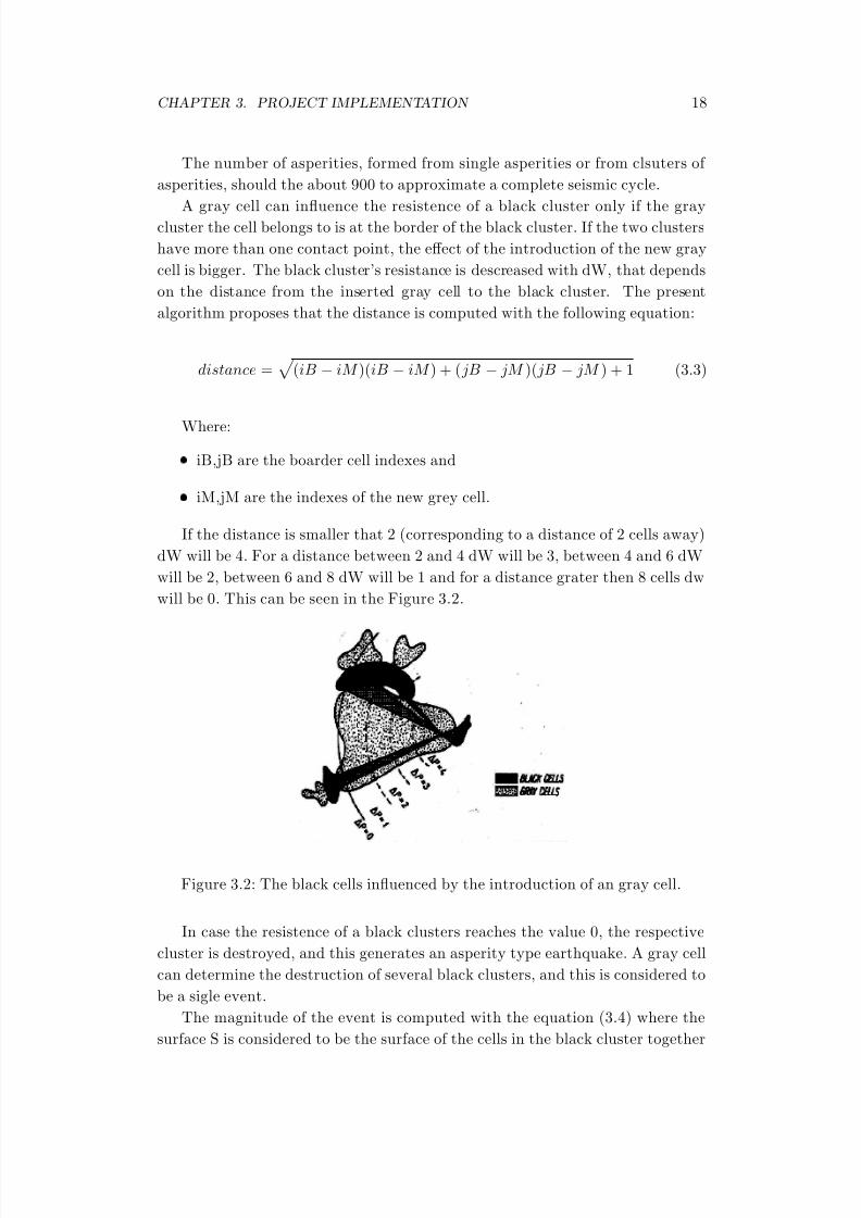
The number of asperities, formed from single asperities or from clsuters of

asperities, should the about 900 to approximate a complete seismic cycle.

A gray cell can influence the resistence of a black cluster only if the graycluster the cell belongs to is at the border of the black cluster. If the two clusters

have more than one contact point, the effect of the introduction of the new gray

cell is bigger. The black cluster’s resistance is descreased with dW, that depends

on the distance from the inserted gray cell to the black cluster. The present

algorithm proposes that the distance is computed with the following equation:

distance =√

(iB − iM )(iB − iM ) + ( jB − jM )( jB − jM ) + 1 (3.3)

Where:

iB,jB are the boarder cell indexes and

iM,jM are the indexes of the new grey cell.

If the distance is smaller that 2 (corresponding to a distance of 2 cells away)

dW will be 4. For a distance between 2 and 4 dW will be 3, between 4 and 6 dW

will be 2, between 6 and 8 dW will be 1 and for a distance grater then 8 cells dw

will be 0. This can be seen in the Figure 3.2.

Figure 3.2: The black cells influenced by the introduction of an gray cell.

In case the resistence of a black clusters reaches the value 0, the respective

cluster is destroyed, and this generates an asperity type earthquake. A gray cell

can determine the destruction of several black clusters, and this is considered to

be a sigle event.

The magnitude of the event is computed with the equation (3.4) where the

surface S is considered to be the surface of the cells in the black cluster together




with the surface of the grey cells that contributed to the event. Asperity type

earthquakes determines black cells to change their state and become white cells.

3.4.4 Percolation type events

A major earthquake can take place in the moment the number of gray cells has

reached a critical level - the number of gray cells is grater than half the total

number of cells. Another condition is that the magnitude of the event is higher

than 6.5. The rupture of an asperity clusters with a big resistence generates a

chain reaction, that causes a major faulting. Then, the remaining black clusters

are analyzed and, for each of them, if its resistence is less than one third of its

resistence before the event, it is considered to be destroyed. The effect of the

destroyed clusters is also taken into account. So, the total magnitude of the

major event increases with each surface of the black cells and grey cells that

contributed to the major events. A seismic cycle ends in the moment a major

event occures.

3.5 Healing process

The existence of the seismic cycles in well defined geographical regions shows on

one hand that there is a process of destruction of the area, that makes possible

the generation of major faulting, and on the other hand that it also exists an

antagonistic process of the healing of the area, that makes possible the beginning

of a new seismic cycle.

Simulated cycle lasts 30-40 years which corresponds to the average seen in

Vrancea cycles. To see the evolution of earthquakes in time and what we could

expect for the next period of seismic activity related to our country, we imple-

mented a mechanism to restore the area affected by earthquakes. Thus, simula-

tion is no longer limited to a single seismic cycle.

To explain the healing of the rupture zones, we should analyze many aspects

as: time, frictional strengthening, fluid variations or changes in the state of stress

as well as the normal compaction of the rupture zone [LV01].

The predicted maximum possible magnitude is M = 7.8 for the upper and

lower active segment, respectively, estimated using the total surface of the active

seismic area for the two segments [RPCR08]. Because of this, the simulation of

a seismic cycle ends when the magnitude of an events is between 7.0 and 7.8,

but not before we see which clusters are also destroyed because of the event (its

magnitude is lower than 13 of its magnitude before the event).

The implementation of healing process takes into account the fact that, during

the weakning process, the stress is being cumulated on a surface that corresponds

to an asperity cluster. The stress is released in the moment an earthquake takes

place. It should pass some time, until the stress is cumulated again, so another




event could occur. So, the place where the earthquake appeared must have a

high resistence in order to cumulate the stress.

At the end of a seismic cycle, we see all the undestroyed clusters, and for eachof it, we verify if its first cell is black (it could also be gray, because the gray cell

form clusters as well). So, for each black cluster, we save all its cells in an array,

and the its resistence in another array. The vector of cells and the resistence of

the undestroyed clusters will be used in the next cycle for the initialization of the

grid.

We consider that if the insertion of a gray cell causes the occuring of an event,

the id of that cell will be the location of an earthquake. When an earthquake

occures, we save its position in grid (its id) in an array that will be used in the

following cycle when we will initialize the grid. Also, we should pay attention

to the magnitude of the event. We tried to differentiate between earthquakesmagnitudes so that better results are obtained.

After the number of clusters begins to decrease due to aggregation, we insert

monoclusters, with the condition that they remain isolated until we reach the

number of 900 clusters, number required for a seismic cycle in the Vrancea zone.

At this time the grid is completely initialized to simulate a new cycle and can

follow the same algorithm as in the case of a single simulation cycle. Basically,

iterative procedure can be applied to simulate several seismic cycles.

We create a file for each seismic cycle in which we write the magnitude of

the events and the location of the earthquake within the grid (line and column),

so the events can be visualized and analyzed. Also for each seismic cycle wecompute graphics with the Gutenberg-Richter law and with the relation between

magnitude and the events order.

To find the distribution in time of the events that occured during a seismic

cycle we take into account the fact that the rate of the background earthquakes

is 50 per year and of asperity type earthquakes is 20-25 per year (consider 25).

Several tests have been made with different methods of computing the re-

sistence of the events from the previous cycle depending of their magnitude. A

version of implementing the healing process proposed in [CPG+07] considers

that the cells inserted after the introduction of the cells from the undestroyed

clusters from the previous cycle should not be coupled with those clusters, but if we do so, we would not heal all the areas where events occured in the previous

cycle.

Because a complete implementation of the healing process should take into

account all the temporal, spatial, physical and chemical features of the seismic

zone and this is very hard, all solutions can be considered good, if satisfactory

results are obtain (closer to the reality).



Chapter 4

Case studies

The scaling relations, such as frequency - magnitude distribution, can provide

valide information as concerns the distribution and evolution of the local stress

field in correlation with the evolution of the geodynamic system.

In order to study the noise of earthquakes, it was needed a way to measure

the size of earthquakes, and so Charles Richter developed the main scale that

is used today. On the Richter scale, the magnitude of an earthquake is propor-

tional to the logaritm of the maximum amplitude of the earths motion. This

means that, in a magnitude 2 earthquake the earth moves one millimeter, in a

magnitude 3 earthquake it will move 10 millimeters, in a magnitude 4 earthquake

100 millimeters, and in a magnitude 6 earthquake 10 meters. So in the magnitude

8 earthquake the ground is moving 10,000 times more than in the magnitude 4

earthquake. Also, it appears a difference in energies that is even greater. For each

factor of 10 in amplitude, the energy grows by a factor of 32, so a magnitude 8

earthquake releases 1,000,000 times more energy than a magnitude 4 earthquake.

The release of energy expalains why the earthquakes do so much damage.

4.1 Gutenberg Richter Law

In seismology, the Gutenberg-Richter law (4.1) expresses the relation between the

magnitude and total number of earthquakes in any given region and time period.

log N = a− bM (4.1)

Where:

N is the number of events with magnitude grater than M that occure in a

given time period,

21



CHAPTER 4. CASE STUDIES 22

M is the minumum magnitude,

a and b are constants.

The constant a depends on the number of earthquakes in the time and region

sampled and the slope b is typically equal to 1.0. This means that for every

magnitude 4.0 event there will be 10 magnitude 3.0 quakes and 100 magnitude 2.0

quakes. A notable exception is during earthquake swarms when the b-value can

become as high as 2.5 indicating an even larger proportion of small quakes to large

ones. A b-value significantly different from 1.0 may suggest a problem with the

data set (it is incomplete or contains errors in calculating magnitude). The the b-

value is an indicator of the completeness of the data set at the low magnitude end.

The Gutenberg-Richter law parameters considered for the simulations are a=5.4

and b=0.88. The red points show the ideal Gutenberg - Richter distribution.

4.2 Real catalogue

The active area that is considered for the simulation is the lower active part of

the slab imagined as the median plane of the earthquakes epicenter. The id of

each activated cell (black cell) is written to a file. These ids will be used for the

initial configuration of the grid.

4.2.1 Initialization

For the initialization of the grid the cells inserted were read from the real cata-

logue of earthquakes. The configuration of the grid after the insertion of the cells

(891 cells) can be seen in Figure 4.1.

Figure 4.1: The cells from the real catalogue of earthquakes.




Figure 4.4 shows the grid after the insertion of the cells that represent the

epicenters of the earthquakes that occured in the first seismic cycle. There are

some cells that were added to the asperity clusters that were not destroyed in theprevious seismic cycle.

Figure 4.4: The grid after the insertion of the earthquakes epicenter.

Then, we insert 800 monoclusters (as we did in the first seismic cycle). We

do not save the undestroyed monoclusters from a cycle to another because they

are only used for the generation of background events. The grid after the reini-

tialization for the second seismic cycle is shown in the Figure 4.5.

Figure 4.5: The grid after the reinitialization for a new seismic cycle.

In this moment the grid is completly reinitialized and the simulation of a new

seismic cycle can begin.




4.2.3 Gutenberg-Richter law

After each seimic cycle we compute the Gutenberg-Richter law. This law shows

the frequency-magnitude distribution for the earthquakes that occur during aseismic cycle. The red points show the ideal Gutenberg - Richter distribution.

Figure 4.6 shows the Gutenberg-Richter distribution for the first seismic cycle.

The initialization of the grid was made from real catalogue of earthquakes.

3.6 3.8 4 4.2 4.4 4.6 4.8 5 5.2 5.40.5

1

1.5

2

2.5

Gutenberg-Richter Law

Figure 4.6: Gutenberg-Richter lawfor the first seismic cycle.

3.6 3.8 4 4.2 4.4 4.6 4.8 5 5.2 5.40.5

1

1.5

2

2.5


Figure 4.7: Gutenberg-Richter lawfor the second seismic cycle.

For the following three seismic cycles the initialization was made with the

cells from the clusters that were not destroyed in the previous seismic cycle and

with cells that represent the epicenters of the earthquakes that occured during the

previous seismic cycle. Figure 4.7 shows the frequency- magnitude distribution for

the second seismic cycle, figure 4.8 shows the frequency-magnitude distribution

for the third one and figure 4.9 shows the frequency-magnitude distribution for

the fourth one.

3.6 3.8 4 4.2 4.4 4.6 4.8 5 5.2 5.40.5

1

1.5

2

2.5


Figure 4.8: Gutenberg-Richter lawfor the third seismic cycle.

3.6 3.8 4 4.2 4.4 4.6 4.8 5 5.2 5.40.5

1

1.5

2

2.5


Figure 4.9: Gutenberg-Richter lawfor the fourth seismic cycle.

The Gutenberg-Richter law is respected by each of the simulated seismic

cycles. Also, it can seen an excces of events with magnitudes lower than 4.0. This

appears because of the big number of monoclusters inserted for the generation of

the background events.




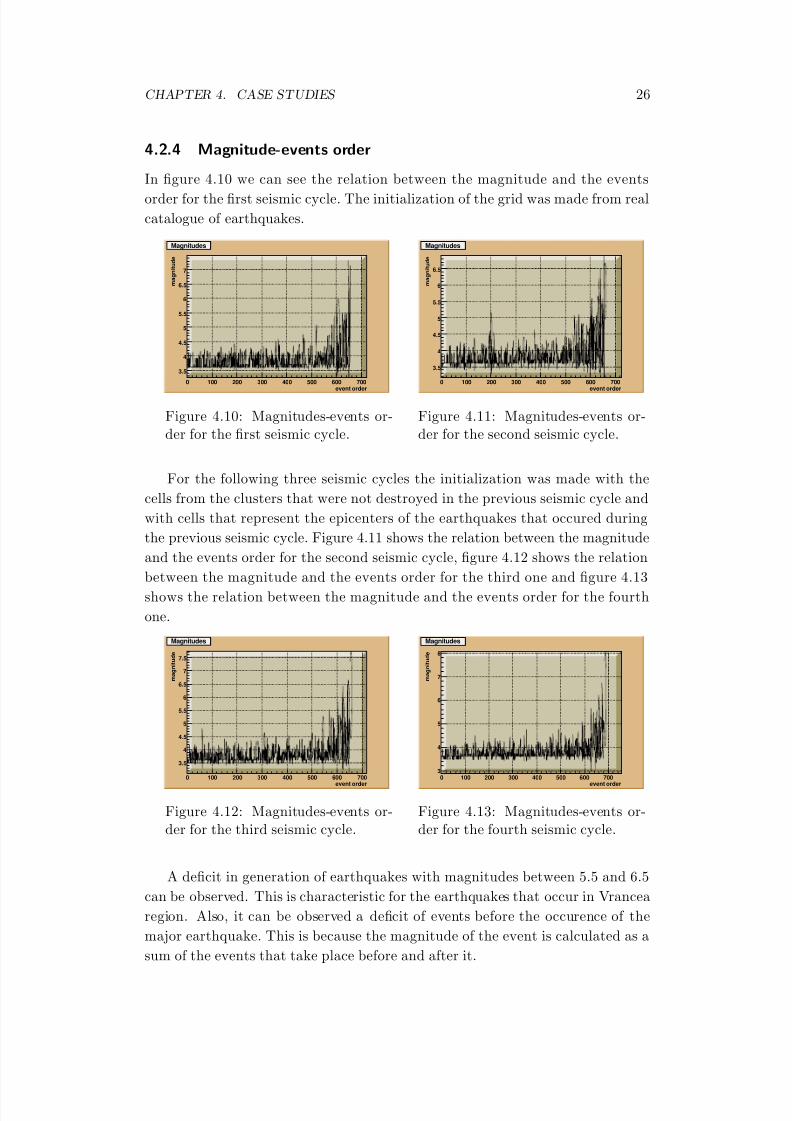
4.2.4 Magnitude-events order

In figure 4.10 we can see the relation between the magnitude and the events

order for the first seismic cycle. The initialization of the grid was made from realcatalogue of earthquakes.

event order0 100 200 300 400 500 600 700

m a g n i t u d e

3.5

4

4.5

5

5.5

6

6.5

7

Magnitudes

Figure 4.10: Magnitudes-events or-der for the first seismic cycle.

event order0 100 200 300 400 500 600 700

m a g n i t u d e

3.5

4

4.5

5

5.5

6

6.5

Magnitudes

Figure 4.11: Magnitudes-events or-der for the second seismic cycle.



with cells that represent the epicenters of the earthquakes that occured during

the previous seismic cycle. Figure 4.11 shows the relation between the magnitude

and the events order for the second seismic cycle, figure 4.12 shows the relation

between the magnitude and the events order for the third one and figure 4.13

shows the relation between the magnitude and the events order for the fourth

one.

event order

0 100 200 300 400 500 600 700

m a g n i t u d e

3.5

4

4.5

5

5.5

6

6.5

7

7.5

Magnitudes

Figure 4.12: Magnitudes-events or-der for the third seismic cycle.

event order

0 100 200 300 400 500 600 700

m a g n i t u d e

3

4

5

6

7

8

Magnitudes

Figure 4.13: Magnitudes-events or-der for the fourth seismic cycle.

A deficit in generation of earthquakes with magnitudes between 5.5 and 6.5

can be observed. This is characteristic for the earthquakes that occur in Vrancea

region. Also, it can be observed a deficit of events before the occurence of the

major earthquake. This is because the magnitude of the event is calculated as a

sum of the events that take place before and after it.




4.2.5 Numerical results

All the events that occur during a seismic cycle are saved to a file. For each event

we save: magnitude, the location in grid (line, column) and the moment (year,month, day) it occured within the seismic cycle. An exemple of a ”simulated

catalogue” can be seen in Figure 4.14. It can be observed a deficit of events

before the occurence of the major earthquake.

Figure 4.14: Simulated catalogue.

In the table 4.1 we can see the results obtained during each of the four seismic

cycles. The second and the third columns contain the number of clusters and the

number of black cells before the insertion of the monoclusters. The last two

columns contain the total number of black clusters and the total number of black

cells.

seismic cycle clusters black cells total clusters total black clusters

first 318 891 880 1453

second 343 912 835 1404

third 363 894 857 1388

fourth 371 832 884 1345

Table 4.1: Results obtained during four seismic cycles.




Then, 800 monoclusters were randomly inserted, so that background events

can take place all over the grid. The configuration of the grid after the insertion

of the monoclusters can be seen in Figure 4.16.

Figure 4.16: The grid in the moment the initialization is finished-1000 trials.

The reinitialization is made exactly as in the case of the previous test.

4.3.2 Gutenberg-Richter law

After each seimic cycle we compute the Gutenberg-Richter law. This law shows

the frequency-magnitude distribution for the earthquakes that occur during aseismic cycle.The red points show the ideal Gutenberg - Richter distribution.

Figure 4.17 shows the Gutenberg-Richter distribution for the first seismic

cycle. The initialization of the grid was made by inserting cells from 1000 trials.

3.6 3.8 4 4.2 4.4 4.6 4.8 5 5.2 5.4

0.5

1

1.5

2

2.5


Figure 4.17: Gutenberg-Richter lawfor the first seismic cycle.

3.6 3.8 4 4.2 4.4 4.6 4.8 5 5.2 5.40.5

1

1.5

2

2.5


Figure 4.18: Gutenberg-Richter lawfor the second seismic cycle.

For the following three seismic cycles the initialization was made with the cells

from the clusters that were not destroyed in the previous seismic cycle and with

cells that represent the epicenters of the earthquakes that occured during the pre-

vious seismic cycle. Figure 4.18 shows the frequency- magnitude distribution for




the second seismic cycle, figure 4.19 shows the frequency-magnitude distribution

for the third one and figure 4.20 shows the frequency-magnitude distribution for

the fourth one.

3.6 3.8 4 4.2 4.4 4.6 4.8 5 5.2 5.40.5

1

1.5

2

2.5


Figure 4.19: Gutenberg-Richter lawfor the third seismic cycle.

3.6 3.8 4 4.2 4.4 4.6 4.8 5 5.2 5.40.5

1

1.5

2

2.5


Figure 4.20: Gutenberg-Richter lawfor the fourth seismic cycle.

The Gutenberg-Richter law is respected by each of the simulated seismic

cycles, but the graphics are not so good as in case the initialization for the first

seismic cycle was made from the real catalogue of earthquakes.

Also, it can seen an excces of events with magnitudes lower than 4.0. This

appears because of the big number of monoclusters inserted for the generation of

the background events.

4.3.3 Magnitude-events order

In figure 4.21 we can see the relation between the magnitude and the events order

for the first seismic cycle. The grid initialized by making 1000 trials to insert cell

(about 900). The figure 4.22 shows the relation between the magnitude and the

events order for the second seismic cycle.

event order0 100 200 300 400 500 600 700

m a g n i t u d e

3.5

4

4.5

5

5.5

6

6.5

7

7.5

Magnitudes

Figure 4.21: Magnitude-events orderfor the first seismic cycle.

event order0 100 200 300 400 500 600 700 800

m a g n i t u d e

3.5

4

4.5

5

5.5

6

6.5

7

Magnitudes

Figure 4.22: Magnitude-events orderfor the second seismic cycle.






with cells that represent the epicenters of the earthquakes that occured during

the previous seismic cycle. Figure 4.23 shows the relation between the magnitude

and the events order for the third seismic cycle and figure 4.24 for the fourth one.

event order0 100 200 300 400 500 600 700 800

m a g n i t u d e

3.5

4

4.5

5

5.5

6

6.5

7

Magnitudes

Figure 4.23: Magnitude-events orderfor the third seismic cycle.

event order0 100 200 300 400 500 600 700

m a g n i t u d e

3.5

4

4.5

5

5.5

6

6.5

7

Magnitudes

Figure 4.24: Magnitude-events orderfor the fourth seismic cycle.

For this test case, a deficit in generation of earthquakes with magnitudes

between 5.5 and 6.5 be also be observed. This is characteristic for the earthquakes

that occur in Vrancea region. Also, it can be seen a deficit of events before the

occurence of the major earthquake. This is because the magnitude of the event

is calculated as a sum of the events that take place before and after it.

4.3.4 Numerical results

In the Table 4.3 we can see the results obtained during each of the four seismic

cycles. The second and the third columns contain the number of clusters and

the number of black cells after the initial configuration of the grid. The last two

columns contain the total number of black clusters and the total number of black

cells.

seismic cycle clusters black cells total clusters total black clusters

first 420 921 872 1373

second 404 712 986 1294

third 437 753 958 1274

fourth 421 759 959 1297Table 4.3: Results obtained during four seismic cycles-1000 trials.

In the Table 4.4 we can see the magnitude of the event after it met the

condition that its magnitude >6.5 and other cluster were destroyed because of

its influence (its magnitude increases with each surface of a destroyed cluster),

the magnitude in the moment it was labeled as a major event and the moment

it occured (year, month, day).




seismic cycle major percolation/magnitude year month day

first 7.189631/6.887674 39 3 24

second 6.863799/6.863799 56 10 22

third 7.130784/6.522183 38 9 7

fourth 6.979730/6.798374 39 2 13

Table 4.4: Major events magnitude during four seismic cycles-1000 trials.

The number of events that occured during each seismic cycles are: 678, 751,

738 and 725. In the second test case, for the last three seismic cycles, the number

of events that occured during each seismic cycle is higher than the one obtained

for the first test case and the magnitudes of the major events are lower.



CHAPTER 5. CONCLUSIONS 34

of earthquake with magnitude 3.6 that can be seen in the simulated catalogue.

This leads to a deviation in the Gutenberg-Richter law for lower magnitudes.

It can be observed a deficit of events before the occurence of the major earth-quake. This is because the magnitude of the event is calculated as a sum of the

events that occure before and after it. Also, a deficit in generation of earthquakes

with magnitudes between 5.5 and 6.5 can be observed. This is characteristic for

the earthquakes that occure in Vrancea region.

Major events in the lower segment of the active area are consideres to have

magnitudes in the range 6.5-7.8. From the test that have been made, the magni-

tudes of the major earthquakes that occured are between 6.86 and 7.62.

The simulated seismic cycles lasted between 38 and 41 years (only one seismic

cycle lasted 56 years). This respects the characteristic return period for the

Vrancea region.



Chapter 6

Future work

The present simulation is only for the lower lithosphere in the Vrancea region.

A simulation that takes into account the hole active area of the Vrancea region

can be made or a simulation for the upper part of the active zone, so that an

evolution of the entire seismic area can be vizualized and analyzed.

The median plane was computed for the hole active area, and from this it

was taken the lower part so that the grid can be initialized. Better result can be

obtained if the plane is computed only for the lower segment of the active area.

Another subject of the future work is represented by finding other methods

to simulate the healing process, so that better results are obtained. For each

method it must be analyzed if the simulation can not lead to configurations that

gradually block the areas capable of being destroyed or, contrary, that gardually

reduce the ability of the system to generate large earthquakes.

All earthquakes occurring along the simulation are introduced in a catalog of

”simulated” earthquakes, so that the data can be viewed and analyzed. Since the

simulation is done using a 2D grid, for each earthquake obtained we only know the

magnitude, the position in the grid and the moment it occured within the seismic

cycle (year, month, day). To see a 3D representation of the earthquakes that

occured during the simulation, it should be made a mechanism of recomputing

the depth depending on the initial projection on the median plane.

The achievement of realistic models for numerical simulation of the physical

and dynamical process of earthquake generation in Vrancea zone is a challenge for

the most advanced research in seismology, taking into account the phenomenon

complexity and multiple scales involved. The realistic simulation proves to be a

powerful tool for investigating the seismic process, understanding the precursory

phenomena and the seismic cycle.

35



Bibliography

[AT08] Ravi Kumar ACAS and Arun Tripathi. Root: A data analysis and data

mining tool from cern. Casualty Actuarial Society E-Forum , pages 24–25,

Winter 2008. [cited at p. 13]

[CPG+07] O. Carbunar, M. Popa, B. Grecu, B. Zaharia, and C. Neagoe. Modelarea real-

ista a procesului seismic din zona vrancea prin simularea numerica a ciclurilor

seismice. INFP, 2007. [cited at p. 7, 12, 20]

[FG98] R. Frisch and R. Garbacea. Slab in the wrong place: Lower lithospheric mantle

delamination in the last stage of the Eastern Carpathian subduction retreat. ,

volume 26 of 7 . Geology, Geology, 1998. [cited at p. 10]

[IH06] M. Imoto and N. Hurukawa. Assessing potential seismic activity in Vrancea,

Romania, using a stress-release model . Earth Planets Space, 2nd edition,2006. [cited at p. 4]

[Int04] International Symposium on Predictability of Evolution and Variation of

the Multiscale Earth System. The Use of Computer Simulations for De-

veloping Earthquake Prediction Technology . John B. Rundle, January 2004.

[cited at p. 8]

[Jia96] Jianwu Jiao. Microscopic and macroscopic cellular-automaton simulations

of fluid flow and wave propagation in rocks. Master’s thesis, University of

Sackatchewan, Sasktoon, 1996. [cited at p. 15]

[KZE+09] I. Koulakov, B. Zaharia, B. Enescu, M. Radulian, M. Popa, S. Parolai, and

J. Zschau. Delamination or slab detachment beneath vrancea? new argu-ments from local earthquake tomography. G-cube, pages 4–7, November 2009.

[cited at p. 8]

[LV01] Yong-Gang Li and John E. Vidale. Healing of the shallow fault zone from

1994-1998 after the 1992 M 7.5 Landers, California, earthquake, volume 28

of 15 . Geophysical Research Letters, 1st edition, August 2001. [cited at p. 19]

[Nad09] N. Nadejde. Earthquake simulation in Vrancea . PhD thesis, University Po-

litehnica of Bucharest, June 2009. [cited at p. 12, 15]

36



BIBLIOGRAPHY 37

[Pas09] A. Pasatoiu. Seismicity catalogue analysis for Vrancea earthquakes. PhD

thesis, University Politehnica of Bucharest, June 2009. [cited at p. 11]

[RPCR08] M. Radulian, M. Popa, O. Carbunar, and M. Rogozea. Seismicity patternsin Vrancea and the predictive features, volume 43. Acta Geod. Geoph. Hung.,

2-3 edition, 2008. [cited at p. 6, 14, 19]

[ZH03] Zoya Zarifi and Jens Havskov. Characteristics of dense nests of deep and

intermediate- depth seismicity . Advances in Geophysics, 2nd edition, 2003.

[cited at p. 5]

[ZW01] D. Zedde and M. Wortel. Shallow slab detachment as a transient source of

heat at midlithospheric depths, volume 20 of 6 . Tectonics, December 2001.

[cited at p. 9]

earthquake simulation

Documents