earthquake forecasting: a possible solution considering

Nat. Hazards Earth Syst. Sci., 11, 3263–3273, 2011www.nat-hazards-earth-syst-sci.net/11/3263/2011/doi:10.5194/nhess-11-3263-2011© Author(s) 2011. CC Attribution 3.0 License.

Natural Hazardsand Earth

System Sciences

Earthquake forecasting: a possible solution considering the GPSionospheric delay

M. De Agostino and M. Piras

Politecnico di Torino, Land, Environment and Geoengineering Department (DITAG) – Corso Duca degli Abruzzi 24,10129 Turin, Italy

Received: 3 August 2011 – Revised: 18 October 2011 – Accepted: 18 October 2011 – Published: 12 December 2011

Abstract. The recent earthquakes in L’Aquila (Italy)and in Japan have dramatically emphasized the problemof natural disasters and their correct forecasting. Oneof the aims of the research community is to find apossible and reliable forecasting method, considering allthe available technologies and tools. Starting from therecently developed research concerning this topic andconsidering that the number of GPS reference stationsaround the world is continuously increasing, this studyis an attempt to investigate whether it is possible to useGPS data in order to enhance earthquake forecasting. Insome cases, ionospheric activity level increases just beforeto an earthquake event and shows a different behaviour5–10 days before the event, when the seismic event hasa magnitude greater than 4–4.5 degrees. Considering theGPS data from the reference stations located around theL’Aquila area (Italy), an analysis of the daily variations ofthe ionospheric signal delay has been carried out in orderto evaluate a possible correlation between seismic eventsand unexpected variations of ionospheric activities. Manydifferent scenarios have been tested, in particular consideringthe elevation angles, the visibility lengths and the time ofday (morning, afternoon or night) of the satellites. In thispaper, the contribution of the ionospheric impact has beenshown: a realistic correlation between ionospheric delay andearthquake can be seen about one week before the seismicevent.

1 Introduction

Earthquake physics is a very complex and broad topic. Itinvolves many scales of the Earth’s crustal structure, rangingfrom tectonic plates to the microscopic processes involved

Correspondence to:M. De Agostino([email protected])

in the friction, generation of electric charges and chemicalreactions.

The Earth’s crust is the rigid external shell of our planet,and it consists of the continental and the oceanic crusts.The slow movement of these plates over the asthenospherelayer and the ocean floor extension is called plate tectonics.The movements of these plates, such as a collision ofthese plates one under another (convergent or subductionboundaries) or a plate separation (divergent boundaries),lead to a strain accumulation within the Earth’s crust,to mechanical deformations and crust rupture when thedeformation exceeds the mechanical strength limit.

The intensity of an earthquake is estimated from theoscillations that are created by different kinds of seismicwaves (usually, surface and body waves).

The mechanism which controls the generation of anearthquake is still not well known. Many theories have beensuggested, starting with the early “Elastic Rebound Theory”(Reid, 1911), SOC theories (Main 1995), up to the latest onewhich states that an earthquake is “a frictional phenomenonrather than a fracture one” (Scholz, 1998).

The term “earthquake forecasting” refers to the knowledgeof the earthquake prognostic parameters – the location, thetime of occurrence and its magnitude – for some timebefore it takes place. The prognostic time window can bedistinguished as: long-term, referring to a time window ofsome decades of years; medium-term, referring to a timewindow of a few years (2–3); and short-term, referring toa time window on the order of up to a couple of months;while the term “immediate” is sometimes used when the timewindow is on the order of a few days.

The scientific literature which concerns earthquakeforecasting is composed of several numbers of papers. Sincethe mid 1970s, in fact, seismologists have been confidentthat earthquake prediction could be achieved within a shortperiod of time (Cicerone et al., 2009). This assumption is theresult of the first successful prediction of a large earthquakein Haicheng – China (1975), with a the magnitude equal to

Published by Copernicus Publications on behalf of the European Geosciences Union.

http://creativecommons.org/licenses/by/3.0/

3264 M. De Agostino and M. Piras: Earthquake forecasting

7.4. Over the last half century, some ionospheric variability,observed for hours to days before the earthquake, has beensuggested as an ionospheric precursor (Pulinets et al., 2004;Zakharenkova et al., 2006; Xu et al., 2011). However, eventoday the possibility to identify ionospheric precursors iscontroversial. One of the key points is whether it is possibleto distinguish the solar, geomagnetic (Duma and Ruzhin,2003) and even tropospheric contributions from the observedionospheric variability in order to identify likely precursorionospheric signatures.

The purpose of this paper is to evaluate the efficacyof the ionospheric Total Electron Content (TEC) as anadditional earthquakes precursor, considering a dramaticItalian case study: the L’Aquila earthquake (6 April 2009,magnitude 6.3). In this paper, Global Positioning System(GPS) data from some reference stations close to theearthquake epicentre are used in an “one-way” positioningalgorithm. This procedure allows to separate the GPSsignal ionospheric propagation delay (directly correlatedwith the TEC) from the geometric errors (i.e. multipaths,random errors) and the propagation delay due to gases in thetroposphere.

In the following, after a short review about some possibleearthquake precursors, the “one way” positioning algorithmused to compute the GPS ionospheric delay is describedin detail. The case study (L’Aquila earthquake) and thecomputation method are presented in the second part. Acomparison between the obtained results and the effectiveearthquake map concludes the paper.

2 Earthquake forecasting: some possible precursors

In order to predict an earthquake and in particular to identifyan effective earthquake precursor, many different physicalquantities and mechanisms have been studied (Eftaxias et al.,2011). Some of the observations realized before a strongearthquake are: the seismic gap, that is the absence ofnormal seismicity in a seismogenic area for a long period(e.g. Papadopoulos et al., 2010), seismic quiescence, that isthe drop in seismicity below its normal level, the changein Earth resistivity (e.g. Dologlou, 2008), the emission ofelectro-magnetic waves (e.g. Gladychev et al., 2001), theincrease in Radon emission from the ground (e.g. Richon etal., 2003), geodetic variations (abnormal ground elevations,e.g. Sobolev, 2011), changes in the chemical composition ofunderground water (e.g. Ryabinin et al., 2011), change intemperature of the aquifers, changes in the Earth’s magneticfield, changes in the Earth’s electric field (e.g. Konstantaraset al., 2008), observed changes in the electron density of theionosphere, and strange animal behaviour, to name some ofthe most important and well-known.

First, the precursors should be ranked in two categories:the time of appearance before the earthquake and theirconfidential merit. All available seismic information should

be used, starting from the seismic regioning, calculationof the seismic risk, and finishing with the most recenttechniques based on the self-organized criticality. Thecumulative principle should be used, adding each newindication that appears to the expert alarm system. Theshort-term precursors, including all types of physical,geochemical, electromagnetic and biological monitoring,should be finally processed.

2.1 Radon emissions

Radon emission monitoring is one of the most widely usedgeological study techniques. As it is known, Radon isthe product of radium decay. Radon is an ideal indicatorin geological research because it is generated continuouslyin any geological structure. Its concentration loss due todecay and due to migration into the atmosphere is alwayscompensated by a new production. The loading-unloadingprocess during earthquake preparation is the reason forRadon concentration variations before an earthquake. Manyauthors, such as Teng (1980), Hauksson (1981), Talwani etal. (1981) and Richon et al. (2003), studied Radon variationsbefore earthquakes and used them as a short-term earthquakeprecursor.

Most of the Radon anomalies began within 30 days ofthe earthquake, even though there does not appear to be anydiagnostic behaviour of either the beginning or the end ofa gas anomaly that gives a consistent clue about when anearthquake is going to happen.

2.2 Groundwater level change observations

Changes in groundwater levels have been observed beforecertain earthquakes and are believed to be in response toa volumetric strain in the Earth’s crust (Cicerone et al.,2009). Many of the characteristics of the groundwaterchange precursors documented in this study, such as thetime of the initialization of the anomalies, the dependenceof the amplitude of the anomaly and epicentral distance,seem to parallel the same characteristics as in the Radon gasanomalies.

2.3 Surface deformations

There has been longstanding interest in looking for surfacedeformations (uplifts, downdrops, tilts, strains, strainrate changes, etc.) before earthquakes (Rikitake, 1976).Many crustal earthquakes, with magnitudes equal to orgreater than 6, have been associated with Earth surfacedeformations.

Surface levelling and laser-ranging geodetic measure-ments are the most accurate way to document grounddeformations over regions that are tens of kilometresin dimension. However, such measurements are timeconsuming and expensive, and the feasible time betweenindividual measurements is from months to years.

Nat. Hazards Earth Syst. Sci., 11, 3263–3273, 2011 www.nat-hazards-earth-syst-sci.net/11/3263/2011/

M. De Agostino and M. Piras: Earthquake forecasting 3265

Fig. 1. Electron and neural density trends for upper ionosphere.

However, modern GPS and satellite-based SAR interfer-ometry measurements are now available to produce geodeticposition changes with individual measurements separatedby minutes to days. The reported deformations took placemonths to days before the earthquakes, and the largestamplitude strains and tilts seem to be associated with thelargest earthquakes.

2.4 Electromagnetic phenomena

Earthquake preparation is usually accompanied by electro-magnetic phenomena in different frequency bands (Uyeda etal., 2009). Summarizing, we can state that before strongearthquakes in fair weather conditions, anomalies of theatmospheric electric field have been observed in the formof electric field increases. According to a previous study(Hao et al., 2000), the time of the anomalous electricfield appearance could be more than one month beforethe earthquake. An objection often put forward againstseismic electric precursory signals is that these signals maybe generated by ionospheric and magnetic anomalies of theEarth’s normal field. Consequently, the question that arises(Koulouras et al., 2009) is: is it possible to discriminateelectrical signals induced by magnetic and ionosphericanomalies from the electrical signals that are generated at thefocal area?

2.5 Ionospheric electron content

The ionosphere is a part of the upper atmosphere where thereare enough electrons and ions to effectively interact withelectromagnetic fields. The electron and neutral densities ofthe upper ionosphere are shown in the Fig. 1 (Pulinets andBoyarchuk, 2004).

The most complete and developed model has been createdfor the observed variations of the electron density inthe ionosphere associated with an earthquake preparationprocess. A complete version of its description can be found

in Pulinets and Boyarchuk (2004). Ionospheric precursorsare part of the more general physical process of earthquakepreparation and it is probably the youngest precursor method.The set of plasma-chemical reactions that start as a result ofionization by Radon involves changes in the water vapourand of the electron content in the near ground layer of theatmosphere.

However, statistical ionospheric precursors lead us to saythat (Pulinets, 2006):

1. Ionopheric variations reveal the local time dependence(in the form of the sign of the critical frequencydeviation from the undisturbed level), as well as“day-before-the-shock” dependence.

2. There exists an earthquake magnitude threshold (equalto 5 degrees) from which the ionosphere starts to “feel”the earthquake preparation process.

3. The anomalous variations in the ionosphere appear, onaverage, within a time interval of 5 to 1 days before theseismic shock.

4. The size of the modified area in the ionosphere increaseswith the magnitude of the earthquake.

The ionospheric effect can be estimated considering differentdata sources, such as the Very Low Frequency (VLF)emissions (Parrot, 1994), ground based measurements ofthe ionospheric precursors of earthquakes (Chen et al.,1999; Pulinets et al., 2002), and local plasma parametermeasurements (Afonin et al., 1999). Different satellitetechniques (topside sounding, ionospheric tomography, radiooccultation) have been realized taking into account themeasurements of the TEC distribution.

In recent years, the use of GPS data derived fromreference stations is becoming a useful way of computinga very detailed TEC map to process the signal ionosphericpropagation delay from satellite to receiver. Many importantand dramatic earthquakes have been analyzed consideringthe TEC variation (Plotkin, 2003; Gahalaut et al., 2006;Huang et al., 2009; Borghi et al., 2009; Singh et al., 2009;Liu et al., 2010; Hasbi et al., 2011). This has led tointeresting results and to confirm that ionospheric activity asan earthquake precursor can be considered.

3 The GPS Ionospheric propagation delay

The GPS carrier phase and pseudorange measurements areaffected by systematic and random errors. There are manysources of systematic errors: satellite orbits, satellite andreceiver clocks, propagation medium, relativistic effects andantenna phase center variations to name only a few (Leick,2004).

The ionosphere, in particular, can be considered as adispersive medium for microwave signals, which means that

www.nat-hazards-earth-syst-sci.net/11/3263/2011/ Nat. Hazards Earth Syst. Sci., 11, 3263–3273, 2011


the propagation velocity and the refractive index for GPSsignals are frequency-dependent. The ionospheric effect hasthe same absolute value for pseudorange and carrier phasemeasurements, but with opposite signs.

Irregularities in the ionosphere produce short-term signalvariations. These scintillation effects may cause a largenumber of cycle slips because the receiver cannot follow theshort-term signal variations and fading periods. Scintillationeffects mainly occur in a belt along the Earth’s geomagneticequator and in the polar auroral zone.

The primary purpose of the second frequency in theGPS satellite constellation is to eliminate the effect of theionosphere on signal propagation. The errors associatedwith ionospheric refraction, in fact, are dependent on thefrequency signal, and thus are different for the L1 andL2 frequencies. They can be eliminated through linearcombinations of them.

The ionosphere may be characterized as that part of theupper atmosphere where a sufficient number of electronsand ions are present to affect the propagation of radiowaves. The spatial distribution of electrons and ions ismainly determined by photo-chemical and transportationprocesses. The state of the ionosphere may be describedby the electron density in units of electrons per cubic meter.The TEC is an important descriptive quantity for the Earth’sionosphere. TEC is the total number of electrons presentalong a path between two points, with units of electronsper square meter, where 1016 electrons m−2

= 1 TEC unit(TECU). Therefore, TEC is directly correlated to the signalionospheric propagation delay, which can be computed, forexample, using a differential network or a precise pointpositioning.

GPS-derived ionosphere models that describe the deter-ministic component of the ionosphere are usually basedon the so-called Single-Layer Model (SLM), as outlinedin Fig. 2. This model assumes that all free electrons areconcentrated in a shell of infinitesimal thickness.

The SLM mapping functionFI may be written using theequation:

FI (z) =1

cosz′with sinz′

=R

R+Hsinz (1)

where:z,z′ are the zenith distances at the height of the stationand the single layer, respectively;

R is the mean radius of the Earth;H is the height of the single layer above the Earth’s

surface.In order to realize a TEC map, the so-calledgeometry-free

linear combination, which principally contains ionosphericinformation, is considered. The equations for un-differencedpseudorange and carrier-phase observables can be written:

P4 = +a

(1

f 21

−1

f 22

)FI (z)E(β,s)+b4

84 = −a

(1

f 21

−1

f 22

)FI (z)E(β,s)+B4

(2)

Fig. 2. Single-Layer Model (from Dach et al., 2007).

where:P4,84 are the geometry-free pseudorange and carrierphase observables (in meters);

a is a constant equal to 4.03×1017 m s−2 TECU−1;f1,f2 are the frequencies associated with the two carrier

phases;FI (z) is the mapping function evaluated at the zenith

distancez (see Eq. 1);E(β,s) is the vertical TEC (in TECU) as a function

of geographic or geomagnetic latitudeβ and sun-fixedlongitudes;

B4,b4 are constant biases (in meters) due to the initialphase ambiguities and to the pseudorange differences,respectively.

“One-way” positioning, or Precise Point Positioning(PPP), is an absolute positioning technique, which is madewithout differential techniques (zero-difference positioning),using data collected by only one receiver, accurate orbital andsatellite clock data and error models of atmospheric delays.The previous equations, referring to a single receiver and asingle satellite, from metric point of view are equal to:

P1 = ρ +c(dt −dT )+T r +I +mP1+eP1P2 = ρ +c(dt −dT )+T r +α×I +mP2+eP281 = ρ +c(dt −dT )+T r −I +λ1N1+m81+e8182 = ρ +c(dt −dT )+T r −α×I +λ2N2+m82+e82

(3)

where:ρ is the range between the receiver and the satellite;c is the speed of light (in meters per second);dt is the satellite clock error;dT is the receiver clock error;Tr is the tropospheric propagation delay;α is the quadratic ratio between the two GPS carrier-phase

frequenciesf1,f2;I is the ionospheric propagation delay;λ1,λ2 are the wavelenghts associated with the two carrier

phases;



Fig. 3. Ionospheric propagation delay.

N is the integer carrier phase ambiguity;mP is the pseudorange multipath delay;m8 is the carrier phase multipath delay;eP are the random errors on pseudorange observables;e8 are the random errors on carrier phase observables.In matrix notation, the previous equations become (Leick,

2004):P1P28182

=

1 1 0 01 α 0 01 −1 λ1 01 −α 0 λ2

ρ +T r +c(dt −dT )

I

N1N2

+

mP1+eP1mP2+eP2m81+e81m82+e82

(4)

It should be noted that this expression is independentof clocks and geometry (receiver and satellite coordinatesand tropospheric delay), and thus gives origin to the namegeometry-free. The objective of this method is to usethis observable in order to estimate the ionospheric signalpropagation delay over the carrier phase and pseudorangemeasurements. In this equation, the effects due to thetropospheric propagation delay and the signal multipath areseparated from the ionospheric contribution. Therefore, thestate vector devoted to solve could be defined consideringthe system at each epoch (“step by step”), or using a Kalmanfilter procedure. In the first case, a raw value of ambiguityis evaluated, whereas in the second case, it is possible toobtain a filtered value of the phase ambiguity that converges,more or less quickly, to an integer value (the so-calledfixedambiguity). The simplest solution in the Kalman Filter isto use a transition matrixF equal to a four-by-four identitymatrix, utilizing the following measurement and systemnoise covariance matrices (meters):

R =

0.30 0 0 0

0 0.15 0 00 0 0.01 00 0 0 0.01

(5)

Q =

502 0 0 00 102 0 00 0 0.12 00 0 0 0.12

(6)

After the Kalman filtering, an observation smoothingcould be performed (calledKalman smoothing). In this way,at each epoch, all measurements are used, and, ultimately,this solution looks like the solution obtained with the LeastSquare method.

The ionospheric propagation delay, in units of distance,computed using the “one-way” positioning for satellitePRN29, using the data from the reference station of L’Aquila(AQUI) is shown in Fig. 3.

The filtering and the smoothing procedures markedlyreduce the RMS values of the ionospheric propagationdelay. In addition, the observations can be weightedwith the satellite elevation angle in order to reduce theinfluence of noise at low elevation angles; this calculationis very important for a single receiver positioning. Theelevation-dependent weight proposed by Huber (2003) isused:

w(z) = cos2z+a ·sin2z (7)

where:z is the satellite zenith distance;a is a coefficient 0a � 1. In this casea = 0.3.

4 Case study: the L’Aquila earthquake

On 6 April 2009, the middle of Italy was subjected to acatastrophic event: a violent earthquake seriously damagedthe Regione Abruzzo (Fig. 4). The main event occurredat 03:32 local time (01:32 UTC), and was rated 6.3 on themoment magnitude scale; its epicentre was near L’Aquila,Abruzzo capital, which, together with the surroundingvillages, suffered the most damage. There had been severalthousand foreshocks and aftershocks since December 2008,more than thirty of which had a Richter magnitude above 3.5.After the main shock, 256 other tremors have been registered.

Following the L’Aquila earthquake, many researchersand research groups have analyzed the available data(GPS measurements, InSAR data) in order to describe thedisplacements and deformations that occurred during theearthquake as clearly as possible.

In addition, some researchers, such as Fidani (2010),Eftaxias (2010), Contoyiannis et al. (2010), Plastino et



Fig. 4. Map of Abruzzo (Italy) and surrounding regions showingthe locations of the epicentres of the earthquakes (M ≥ 4.0) from6 April to 13 April 2009. The black star indicates the main event(M = 6.3) of 6 April 2009.

al. (2010) and Perrone et al. (2010), Pergola et al. (2010),Villante et al. (2010), have attempted to analyze thephenomenon with the purpose of discriminating possibleearthquake precursors (earthquake lights, electromagneticanomalies, uranium groundwater anomalies, ionosphericprecursors) that could have foreseen the seismic event.

Papadopoulos et al. (2010), in particular, used the avail-able earthquake catalogue extending from 1 January 2006 to30 June 2009 to detect significant changes before and afterthe mainshock in the seismicity rate. According to theiranalysis, in the last 10 days before the mainshock, strongforeshock signals became evident in space (dense epicentreconcentration in the hanging-wall of the Paganica fault), intime and in size.

Tsolis and Xenos (2010) use the Cross Correlationanalysis method (Pulinets et al., 2004) with their EmpiricalMode Decomposition method to analyze foF2 signalscollected from three ionospheric stations, in order to verifythe existence of seismo-ionospheric precursors before theearthquake. Their work shows that precursors may appearas early as 22 days prior to the event, and 2 days before themainshock.

The authors have attempted to contribute to this topic bymaking an analysis of the ionospheric propagation delay,where several GPS reference stations located within 100 kmsof the earthquake epicentre have been considered. Themain purpose of this analysis was to analyze whether the

Table 1. Coordinates of the GPS CORSs.

Reference StationApprox. coordinates

Latitude (deg) Longitude (deg)

L’Aquila (AQUI) 42.34 13.38Ascoli Piceno (ASCO) 42.82 13.64Atri (ATRA) 42.55 14.01Castel del Monte (CDRA) 42.37 13.72Montereale (MTRA) 42.53 13.24Monterotondo (MORO) 42.05 12.62Oricola (OCRA) 42.05 13.04Ovindoli (OVRA) 42.14 13.51Sulmona (SMRA) 42.05 13.92Sora (SORA) 41.71 13.60Terni (TERI) 42.57 12.65

Table 2. Earthquake preparation zone radius for differentmagnitudes.

Magnitude Earthquake preparationzone radiusρ (km)

3 19.54 52.55 1416 3807 10228 27549 7413

ionospheric delay computed with a “one way” geometry-freeapproach, using a Kalman filter procedure to model the dailyvariability, which may be used as an additional earthquakeprecursor.

5 Tests

Data from GPS Continuous Operating Reference Stations(CORSs) placed near the earthquake epicentre have beenused to study the trend of the ionospheric propagation delaynear the L’Aquila seismic event. The CORSs that wereconsidered are reported in Table 1 and in Fig. 5.

These stations were chosen according to the earthquakepreparation zone radius with respect to the distance from theepicentre, as described in Table 2 (Dobrovolsky et al., 1979).

GPS data from 15 March (Julian Day 74/2009) to 17 April(JD 107/2009) (15 days before and 15 days after theearthquake) were considered for each station. ConcerningL’Aquila reference station, close to the mainshock epicentre,a larger time window, from between 9 February (JD 40/2009)and 17 April (JD 107/2009), was considered.



Fig. 5. Map of the GPS CORSs in the middle of Italy.

Fig. 6. Elevation of GPS satellites on week 1526 for the AQUI site(15◦ cut-off angle).

“One-way” positioning for each station and every daywere performed, considering three different satellites (PRNs8, 11 and 29) of the GPS constellation. The choice of thesethree satellites was necessary to monitor the behaviour of theionospheric propagation delay during three different parts ofthe day (morning, afternoon and night), as shown in Fig. 6.For this reason, the highest satellite for each part of the daywas considered. The figure indicates the position of thesatellites on the day of the greatest earthquake event (JD

Fig. 7. Screenshots of the developed software.

96/2009), but it can be considered roughly equivalent for theother days of the analysis, as the temporal displacement ofthe satellites is equal to 4 min per day. The three satellitesused in this analysis are highlighted in Fig. 6.

The “one-way” positioning in Eq. (4) has beenimplemented in a Kalman filter, using a dedicated softwaredeveloped in FORTRAN language. The results wereanalyzed by means of some toolboxes that have beendeveloped in MATLAB® language (Fig. 7). The aim ofthese software is to provide an early-warning tool priorto the earthquake phenomena. Broadcasted ephemeris andobservation data from RINEX files with a sampling intervalequal to 30 s were used. The results of the performed analysisare shown in the next section.

6 Results

The ionospheric propagation delay for each reference stationusing the “one-way” positioning described in Sect. 3considering the three GPS satellites PRNs 8, 11 and 29 wascomputed. The AQUI CORS (L’Aquila) was analyzed for alonger time period than the one mentioned in the previoussection, in order to have a longer and more significant timeseries.

A time window from between 9 February (JD 40/2009)and 17 April (JD 107/2009) was considered. The trends ofthe daily average value of the ionospheric propagation delayfor the L’Aquila GPS station are shown in the followingfigures for each chosen satellite. The week before and theweek after the earthquake of 6 April (JD 96/2009) are drawnin red.

Analyzing the figures above, it is possible to identify ananomalous variation in the ionospheric propagation delaypatterns about a week before the seismic event (JD 88/2009),especially for satellite PRN 29 (see Fig. 8). The ionosphericpropagation delays computed for satellites PRNs 11 and 8



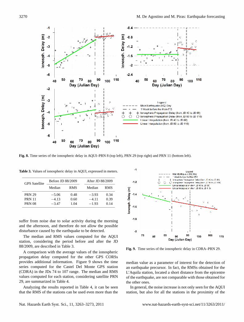
Fig. 8. Time series of the ionospheric delay in AQUI–PRN 8 (top left), PRN 29 (top right) and PRN 11 (bottom left).

Table 3. Values of ionospheric delay in AQUI, expressed in meters.

GPS SatelliteBefore JD 88/2009 After JD 88/2009

Median RMS Median RMS

PRN 29 −5.06 0.48 −3.93 0.34PRN 11 −4.13 0.60 −4.11 0.39PRN 08 −3.47 1.04 −1.93 0.14

suffer from noise due to solar activity during the morningand the afternoon, and therefore do not allow the possibledisturbance caused by the earthquake to be detected.

The median and RMS values computed for the AQUIstation, considering the period before and after the JD88/2009, are described in Table 3.

A comparison with the average values of the ionosphericpropagation delay computed for the other GPS CORSsprovides additional information. Figure 9 shows the timeseries computed for the Castel Del Monte GPS station(CDRA) in the JDs 74 to 107 range. The median and RMSvalues computed for each station, considering satellite PRN29, are summarized in Table 4.

Analyzing the results reported in Table 4, it can be seenthat the RMS of the stations can be used even more than the

Fig. 9. Time series of the ionospheric delay in CDRA–PRN 29.

median value as a parameter of interest for the detection ofan earthquake precursor. In fact, the RMSs obtained for theL’Aquila station, located a short distance from the epicentreof the earthquake, are not comparable with those obtained forthe other ones.

In general, the noise increase is not only seen for the AQUIstation, but also for all the stations in the proximity of the



Table 4. The ionospheric propagation delay for satellite PRN29expressed in meters.

Reference StationBefore JD 88/2009 After JD 88/2009

Median RMS Median RMS

L’Aquila (AQUI) −5.06 0.48 −3.93 0.34Ascoli Piceno (ASCO) −2.93 0.10 −2.89 0.07Atri (ATRA) −5.15 0.10 −5.01 0.11Castel del Monte (CDRA) −4.91 0.12 −4.59 0.19Montereale (MTRA) −5.22 0.10 −5.00 0.13Monterotondo (MORO) −0.51 0.10 −0.45 0.06Oricola (OCRA) −5.87 0.12 −5.59 0.72Ovindoli (OVRA) −5.04 0.11 −4.73 0.11Sulmona (SMRA) −5.52 0.11 −5.30 0.12Sora (SORA) −1.45 0.09 −1.38 0.07Terni (TERI) 0.03 0.09 0.15 0.06

earthquake epicentre. A representation of this phenomenoncan be obtained interpolating the values computed dailyfor each station (e.g. through a simple Kriging, using aMATLAB® toolbox developed by Lophaven et al., 2002).

The spatial variations of the ionospheric propagationdelay, with respect to the median value of the period beforethe JD 88/2009, are shown in Fig. 10.

The behaviour of the ionospheric propagation delayvariation on the JDs 88/2009 and 94/2009 are shown in thefollowing figures.

7 Conclusions and future tests

The developed tests and the relative analysis demonstratethat the ionospheric delay could be an additional precursorof earthquakes.

As demonstrate above, before L’Aquila’s earthquake thestudy of the ionospheric anomalies could be significant,especially around 7 days before the event. Ionosphericvariations and RMS values have been effective precursors ofthe dramatic event of 6 April. A few days before the event,strange variations were observed around the epicentre.

The results are consistent with the previous work of Tsolisand Xenos (2010), showing an anomalous behaviour of theionosphere one week before the mainshock. The possibilityto use GPS and GLONASS CORSs is really interesting, sincedoing so allows densifying the number of observations thatcan be analysed in order to obtain a complete tomography ofthe ionosphere.

The earthquake preparation zone has been correctlydetected as an area with a radius equal to 100 kms withrespect to the epicentre.

The precursor’s characteristics are different in differentseismically active regions. These regional peculiaritiesshould therefore be studied.

The GPS ionospheric propagation delay analysis can beconsidered an appreciable precursor but its limits can be

Fig. 10. Contour plot of the ionospheric delay variation–JD88(top) and JD94 (bottom). Yellow stars show the locations of theearthquakes epicentres (M ≥ 4.0) from 6 April to 13 April 2009.

observed when the value of magnitude is not so high (<5.5).The tremors that occurred before and after the main tremorsare not detected using this approach.

The last conclusion concerns the precursor variation withthe season and solar cyclephase. It is well known that thereare strong variations in the ionosphere parameters accordingto the season and solar cycle. It is quite possible thationosphere sensitivity to the seismic events and the overallprecursor characteristics may also change according to theseason and the cycle phase. The seasonal dependencies couldnot only be due to ionospheric variations, but also to changesin the weather conditions. Winds, rain, snow, and fog mayall contribute to the electric field generation mechanism. Inorder to answer this question, it is necessary to conductfurther investigations, to make other tests and consider otherfactors.



Acknowledgements.The Authors would like to thank the peopleand networks that have kindly made their GPS reference stationsdata available, and in particular Leica ItalPoS, the networks ofreference stations of Regione Abruzzo and Regione Umbria andthe RESNAP-GPS CORSs network.

Edited by: A. CostaReviewed by: K. Eftaxias and another anonymous referee

References

Afonin, V. V., Molchanov, O. A., Kodama, T., Hayakawa,M., and Akentieva, O. A.: Statistical study of ionosphericplasma response to seismic activity: search for reliable resultfrom satellite observations, in: Atmospheric and IonosphericElectromagnetic Phenomena Associated with earthquakes, TerraScientific Publishing Company, Tokyo, Japan, 597–618, 1999.

Borghi, A., Aoudia, A., Riva, R., and Barzaghi, R.: GPS monitoringand earthquake prediction: a success story towards a usefulintegration, Tectonophysics, 465, 177–189, 2009.

Chen, Y. I., Chuo, J. Y., Liu, J. Y., and Pulinets, S. A.: StatisticalStudy of Ionospheric Precursors of Strong Earthquakes at TaiwanArea, XXVI URSI General Assembly, Toronto, Canada, 13–21August 1999, 745, 1999.

Cicerone, R. D., Ebel, J. E., and Britton, J.: A systematiccompilation of earthquake precursors, Tectonophysics, 476,371–396, 2009.

Contoyiannis, Y. F., Nomicosb, C., Kopanasc, J., Antonopoulos,G., Contoyianni, L., and Eftaxias, K.: Critical featuresin electromagnetic anomalies detected prior to the L’Aquilaearthquake, Physica A, 389, 499–508, 2010.

Dach, R., Hugentobler, U., Fridez, P., and Meindl, M. (Eds.): Usermanual of Bernese GPS Software Version 5.0. AstronomicalInstitute, University of Bern, Chapt. 12 “Ionosphere Modelingand Estimation”, 253–278, 2007.

Dobrovolsky, I. R., Zubkov, S. I., and Myachkin, V. I.: Estimationof the size of earthquake preparation zones, Pure Appl. Geophys.,117, 1025–1044, 1979.

Dologlou, E.: Power law relationship between parameters ofearthquakes and precursory electrical phenomena, Nat. HazardsEarth Syst. Sci., 8, 977–983,doi:10.5194/nhess-8-977-2008,2008.

Duma, G. and Ruzhin, Y.: Diurnal changes of earthquake activityand geomagnetic Sq-variations, Nat. Hazards Earth Syst. Sci., 3,171–177,doi:10.5194/nhess-3-171-2003, 2003.

Eftaxias, K.: Footprints of nonextensive Tsallis statistics,selfaffinity and universality in the preparation of the L’Aquilaearthquake hidden in a pre-seismic EM emission, Physica A,389, 133–140, 2010.

Eftaxias, K., Maggipinto, T., and Meister, C.-V.: Progress inthe research on earthquakes precursors, Special Issue, Nat.Hazards Earth Syst. Sci.,http://www.nat-hazards-earth-syst-sci.net/specialissue125.html, 2011.

Fidani, C.: The earthquake lights (EQL) of the 6 April 2009 Aquilaearthquake, in Central Italy, Nat. Hazards Earth Syst. Sci., 10,967–978,doi:10.5194/nhess-10-967-2010, 2010.

Gahalaut, V. K., Nagarajan, B., Catherine, J. K., and Kumar, S.:Constraints on 2004 Sumatra–Andaman earthquake rupture from

GPS measurements in Andaman–Nicobar Islands, Earth Planet.Sc. Lett., 242, 365–374, 2006.

Gladychev, V., Baransky, L., Schekotov, A., Fedorov, E.,Pokhotelov, O., Andreevsky, S., Rozhnoi, A., Khabazin, Y.,Belyaev, G., Gorbatikov, A., Gordeev, E., Chebrov, V., Sinitsin,V., Lutikov, A., Yunga, S., Kosarev, G., Surkov, V., Molchanov,O., Hayakawa, M., Uyeda, S., Nagao, T., Hattori, K., and Noda,Y.: Study of electromagnetic emissions associated with seismicactivity in Kamchatka region, Nat. Hazards Earth Syst. Sci., 1,127–136,doi:10.5194/nhess-1-127-2001, 2001.

Hao, J., Tang, T., and Li, D.: Progress in the research of atmosphericelectric field anomaly as an index for short-impending predictionof earthquakes. J. Earthquake Pred. Res. 8, 241–255, 2000.

Hasbi, A. M., Mohd Ali, M. A., and Misran, N.: Ionosphericvariations before some large earthquakes over Sumatra, Nat.Hazards Earth Syst. Sci., 11, 597–611,doi:10.5194/nhess-11-597-2011, 2011.

Hauksson, E.: Radon Content of Groundwater as an EarthquakePrecursor: Evaluation of Worldwide Data and Physical Basis, J.Geophys. Res., 86, 9397–9410, 1981.

Hayakawa, M.: Atmospheric and Ionospheric ElectromagneticPhenomena Associated with Earthquakes, Terra ScientificPublishing Company, Tokio, Japan, 1999.

Huang, B. S., Huang, W. G., Huang, Y. L., Kuo, L. C., Chen, K.C., and Angelier, J.: Complex fault rupture during the 2003Chengkung, Taiwan earthquake sequence from dense seismicarray and GPS observations, Tectonophysics, 466, 184–204,2009.

Huber, S. and Kaniuth, K.: On the Weighting of GPSPhase Observations in the EUREF Network Processing, in:Proceedings of the Symposium of the IAG Subcommission forEurope (EUREF), Toledo, Spain, 4-7 June 2003, 5, 2003.

King, C. Y.: Gas geochemistry applied to earthquake prediction: anoverview, J. Geophys. Res. 91, 269–281, 1996.

Konstantaras, A., Fouskitakis, G. N., Makris, J. P., and Vallianatos,F.: Stochastic analysis of geo-electric field singularities asseismically correlated candidates, Nat. Hazards Earth Syst. Sci.,8, 1451–1462,doi:10.5194/nhess-8-1451-2008, 2008.

Koulouras, G., Balasis, G., Kiourktsidis, I., Nannos, E.,Kontakos, K., Stonham, J., Ruzhin, Y., Eftaxias, K., Kavouras,D., and Nomikos, C.: Discrimination between pre-seismicelectromagnetic anomalies and solar activity effects, Phys.Scripta, 79, 45901 (12 pp.), 2009.

Leick, A.: GPS Satellite Surveying, 3rd edition, John Wiley & Sons,New Jersey, 2004.

Liu, J. Y., Chen, C. H., Chen, Y. I., Yang, W. H., Oyama, K. I.,and Kuo, K. W.: A statistical study of ionospheric earthquakeprecursors monitored by using equatorial ionization anomaly ofGPS TEC in Taiwan during 2001–2007, J. Asian Earth Sci., 39,76–80, 2010.

Lophaven, S. N., Nielsen, H. B., and Søndergaard, J.: DACE – AMatlab Kriging Toolbox, 2nd version, Technical Report IMM-TR-2002-12, Technical University of Denmark, 2002.

Main, I.: Earthquakes as critical phenomena: implications for theprobabilistic seismic hazard analysis, Bull. Seism. Soc. Am. 85,1299–1308, 1995.

Nikolopoulos, S., Kapiris, P., Karamanos, K., and Eftaxias, K.: Aunified approach of catastrophic events, Nat. Hazards Earth Syst.Sci., 4, 615–631,doi:10.5194/nhess-4-615-2004, 2004.


http://dx.doi.org/10.5194/nhess-8-977-2008


http://www.nat-hazards-earth-syst-sci.net/special_issue125.html

http://www.nat-hazards-earth-syst-sci.net/special_issue125.html








Papadopoulos, G. A., Charalampakis, M., Fokaefs, A., andMinadakis, G.: Strong foreshock signal preceding the L’Aquila(Italy) earthquake (Mw 6.3) of 6 April 2009, Nat. Hazards EarthSyst. Sci., 10, 19–24,doi:10.5194/nhess-10-19-2010, 2010.

Parrot, M.: Statistical study of ELF/VLF emissions recorded bya low altitude satellite during seismic events, J. Geophys. Res.,99–23, 339–347, 1994.

Pergola, N., Aliano, C., Coviello, I., Filizzola, C., Genzano, N.,Lacava, T., Lisi, M., Mazzeo, G., and Tramutoli, V.: Using RSTapproach and EOS-MODIS radiances for monitoring seismicallyactive regions: a study on the 6 April 2009 Abruzzo earthquake,Nat. Hazards Earth Syst. Sci., 10, 239–249,doi:10.5194/nhess-10-239-2010, 2010.

Perrone, L., Korsunova, L. P., and Mikhailov, A. V.: Ionosphericprecursors for crustal earthquakes in Italy, Ann. Geophys., 28,941–950,doi:10.5194/angeo-28-941-2010, 2010.

Plastino, W., Povinec, P., De Luca, G., Doglioni, C., Nisi, S.,Ioannucci, L., Balata, M., Laubenstein, M., Bella, F., and Coccia,E.: Uranium groundwater anomalies and L’Aquila earthquake,6th April 2009 (Italy), J. Environ. Radioactiv., 101, 45–50, 2010.

Plotkin, V. V.: GPS detection of ionospheric perturbation before the13 February 2001, El Salvador earthquake, Nat. Hazards EarthSyst. Sci., 3, 249–253,doi:10.5194/nhess-3-249-2003, 2003.

Pulinets, S. A.: Space technologies for short-term earthquakewarning, Adv. Space Res., 37, 643–652, 2006.

Pulinets, S. A. and Boyarchuk, K.: Ionospheric Precursors ofEarthquakes, Springer Berlin Heidelberg, Germany, 2004.

Pulinets, S. A., Boyarchuk, K., Lomonosov, A. M., Khegai, V.V., and Liu, J. Y.: Ionospheric precursors to earthquakes: apreliminary analysis of the foF2 critical frequencies at Chung-Liground-based station for vertical sounding of the ionosphere(Taiwan island), Geomagn. Aeronom. 42, 508–513, 2002.

Pulinets, S. A., Gaivoronska, T. B., Leyva Contreras, A., andCiraolo, L.: Correlation analysis technique revealing ionosphericprecursors of earthquakes, Nat. Hazards Earth Syst. Sci., 4,697–702,doi:10.5194/nhess-4-697-2004, 2004.

Reid, H. F.: The elastic rebound theory of earthquakes, Bull. Dept.Geology. Univ. California, 6, 413 pp., 1911.

Richon, P., Sabroux, J. C., Halbwach,s M., Vandemeulebrouck,J., Poussielgue, N., Tabbagh, J., and Punongbayan, R.: Radonanomaly in the soil of Taal volcano, the Philippines: a likelyprecursor of the M 7.1 Mindoro earthquake (1994), Geophys.Res. Lett., 30, 1481,doi:10.1029/2003GL016902, 2003.

Rikitake, T.: Earthquake Prediction, Elsevier, New York, USA,1976.

Ryabinin, G. V., Polyakov, Yu. S., Gavrilov, V. A., andTimashev, S. F.: Identification of earthquake precursors inthe hydrogeochemical and geoacoustic data for the Kamchatkapeninsula by flicker-noise spectroscopy, Nat. Hazards Earth Syst.Sci., 11, 541–548,doi:10.5194/nhess-11-541-2011, 2011.

Scholz, C. H.: Earthquakes and friction laws, Nature, 391, 37–42,1998.

Singh, O. P., Chauhan, V., Singh, V., and Singh, B.: Anomalousvariation in total electron content (TEC) associated withearthquakes in India during September 2006–November 2007,Phys. Chem. Earth, 34, 479–484, 2009.

Sobolev, G. A.: Seismicity dynamics and earthquake predictability,Nat. Hazards Earth Syst. Sci., 11, 445–458,doi:10.5194/nhess-11-445-2011, 2011.

Stein, S. and Wysession, M.: An Introduction to Seismology,earthquakes and Earth structure, Wiley-Blackwell Publishing,2003.

Talwani, P., Moore, W., and Chiang, J.: Radon Anomalies andMicroearthquakes at Lake Jocassee, South Carolina, J. Geophys.Res., 85, 3079–3088, 1980.

Teng, T. L.: Some Recent Studies on Groundwater Radon Contentas an Earthquake Precursor, J. Geophys. Res., 85, 3089–3099,1980.

Thanassoulas, C.: Short-Term Earthquake Prediction, H. Dounias& Co, Greece, 2007.

Tsolis, G. S. and Xenos, T. D.: A qualitative study ofthe seismo-ionospheric precursors prior to the 6 April 2009earthquake in L’Aquila, Italy, Nat. Hazards Earth Syst. Sci., 10,133–137,doi:10.5194/nhess-10-133-2010, 2010.

Uyeda, S., Nagao, T., and Kamogawa, M.: Short-term earthquakeprediction: current status of seismo-electromagnetics, Tectono-physics, 470, 205–213, 2009.

Villante, U., De Lauretis, M., De Paulis, C., Francia, P., Piancatelli,A., Pietropaolo, E., Vellante, M., Meloni, A., Palangio, P.,Schwingenschuh, K., Prattes, G., Magnes, W., and Nenovski, P.:The 6 April 2009 earthquake at L’Aquila: a preliminary analysisof magnetic field measurements, Nat. Hazards Earth Syst. Sci.,10, 203–214,doi:10.5194/nhess-10-203-2010, 2010.

Xu, T., Wu, J., Zhao, Z., Liu, Y., He, S., Li, J., Wu, Z., and Hu, Y.:Brief communication “Monitoring ionospheric variations beforeearthquakes using the vertical and oblique sounding networkover China”, Nat. Hazards Earth Syst. Sci., 11, 1083–1089,doi:10.5194/nhess-11-1083-2011, 2011.

Zakharenkova, I. E., Krankowski, A., and Shagimuratov, I. I.:Modification of the low-latitude ionosphere before the 26December 2004 Indonesian earthquake, Nat. Hazards Earth Syst.Sci., 6, 817–823,doi:10.5194/nhess-6-817-2006, 2006.





http://dx.doi.org/10.5194/angeo-28-941-2010



http://dx.doi.org/10.1029/2003GL016902








earthquake forecasting: a possible solution considering

Documents