earth resistivity estimation based on satellite … · earth resistivity estimation based on...
TRANSCRIPT

Earth Resistivity Estimation Based on Satellite Imaging Techniques
KWANCHAI NORSANGSRI and THANATCHAI KULWORAWANICHPONG* Power System Research Unit
School of Electrical Engineering Suranaree University of Technology
111 University Avenue, Nakhon Ratchasima THAILAND
* Corresponding author, [email protected]
Abstract: - This paper proposes a useful technique for generating an earth resistivity map. Earth resistance is one of essential factors in a broad range of power system analysis and design. Information of earth resistivity is helpful for practical power system engineers in order to establish power system grounding. In this paper, a LANSAT7 image of a tested area of 50 km2 was used by ENVI program in associative with a set of resistivity data obtained from field measurement. By using the maximum likelihood for supervised classification of a mixed band 7, 5 and 3, highest value of 85.71% confidence was obtained. Key-Words: - Earth resistivity, Wenner method, Satellite image technology, Power system grounding, Classification technique, Multispectral 1 Introduction Satellite images have found their several applications [1-5] in fields of agriculture, geology, forestry, biodiversity conservation, regional planning, education, intelligence, warfare, weather forecast, electric power system, etc. Images can be in visible colors and in other spectra. To interpret and analyze satellite images, some efficient software packages like ERDAS or ENVI are necessary. All satellite images produced by NASA are published by Earth Observatory and are freely available to the public. Several other countries, nowadays, have satellite imaging programs, and a collaborative European effort launched the ERS and Envisat satellites carrying various sensors. There are also private companies that provide commercial satellite imagery. In the early 21st century satellite imagery became widely available when affordable, easy to use software with access to satellite imagery databases became offered by several companies and organizations. Satellite Image Technology or Remote Sensing has guided the way to the development of hyperspectral and multispectral sensors around the world as a useful tool that can be used to map specific materials by detecting specific chemical and material bonds from satellite and airborne sensors. Multispectral data obtained in space by those sensors have been exploited extensively for the past several years in a wide range of research projects such as land cover and topographic mapping, physical and biological oceanography, archaeology, etc. Research has expanded to include analysis of hyperspectral data acquired simultaneously in tens to hundreds of narrow channels. New algorithms have been developed both to exploit the spectral information of these sensors and to
better deal with the computational demands of these enormous data sets. It is an excellent tool for environmental assessments, mineral mapping and land cover mapping, wildlife habitat monitoring and general land management studies. Multispectral imaging often can include large data sets and require specialized processing methods. In this paper, satellite images have been brought to estimate earth resistivity that can be used extensively in applications of power system grounding. Hyperspectral data sets of satellite images are generally composed of about 100 to 200 spectral bands of relatively narrow bandwidths (5-10 nm), whereas, multispectral data sets are usually composed of about 5 to 10 bands of relatively large bandwidths (70-400 nm). Actual detection of materials is dependent on the spectral coverage, spectral resolution, and signal-to-noise of the spectrometer, the abundance of the material and the strength of absorption features for that material in the wavelength region. In remote sensing situations, the surface materials mapped must be exposed in the optical surface and the diagnostic absorption features must be in regions of the spectrum that are reasonably transparent to the atmosphere. With these assumptions, it is possible to employ satellite images in order to visualize earth resistivity of the earth surface. This paper consists of five main sections. Section 2 gives explanation of earth resistivity and its measurement. Section 3 covers a brief of satellite image processing. Results and discussion are put in Section 4. Section 5 presents a conclusion remark and further work.
WSEAS TRANSACTIONS on SYSTEMS Kwanchai Norsangsri, Thanatchai Kulworawanichpong
ISSN: 1109-2777 1061 Issue 9, Volume 8, September 2009
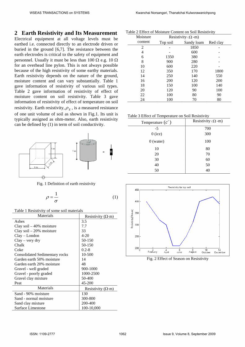
2 Earth Resistivity and Its Measurement Electrical equipment at all voltage levels must be earthed i.e. connected directly to an electrode driven or buried in the ground [6,7]. The resistance between the earth electrodes is critical to the safety of equipment and personnel. Usually it must be less than 100 Ω e.g. 10 Ω for an overhead line pylon. This is not always possible because of the high resistivity of some earthy materials. Earth resistivity depends on the nature of the ground, moisture content and can vary substantially. Table 1 gave information of resistivity of various soil types. Table 2 gave information of resistivity of effect of moisture content on soil resistivity. Table 3 gave information of resistivity of effect of temperature on soil resistivity. Earth resistivity, Eρ , is a measured resistance of one unit volume of soil as shown in Fig.1. Its unit is typically assigned as ohm-meter. Also, earth resistivity can be defined by (1) in term of soil conductivity.
Fig. 1 Definition of earth resistivity
σρ 1= (1)
Table 1 Resistivity of some soil materials
Materials Resistivity (Ω⋅m) Ashes 3.5 Clay soil – 40% moisture 7.7 Clay soil – 20% moisture 33 Clay – London 4-20 Clay – very dry 50-150 Chalk 50-150 Coke 0.2-8 Consolidated Sedimentary rocks 10-500 Garden earth 50% moisture 14 Garden earth 20% moisture 48 Gravel - well graded 900-1000 Gravel - poorly graded 1000-2500 Gravel clay mixture 50-400 Peat 45-200
Materials Resistivity (Ω⋅m) Sand - 90% moisture 130 Sand - normal moisture 300-800 Sand clay mixture 200-400 Surface Limestone 100-10,000
Table 2 Effect of Moisture Content on Soil Resistivity Moisture content
Resistivity (Ω -m) Top soil Sandy loam Red clay
2 - 1850 - 4 - 600 - 6 1350 380 - 8 900 280 -
10 600 220 - 12 350 170 1800 14 250 140 550 16 200 120 200 18 150 100 140 20 120 90 100 22 100 80 90 24 100 70 80
Table 3 Effect of Temperature on Soil Resistivity Temperature )(c Resistivity (Ω -m)
-5 700 0 (ice) 300
0 (water) 100
10 80 20 70 30 60 40 50 50 40
Fig. 2 Effect of Season on Resistivity
WSEAS TRANSACTIONS on SYSTEMS Kwanchai Norsangsri, Thanatchai Kulworawanichpong
ISSN: 1109-2777 1062 Issue 9, Volume 8, September 2009
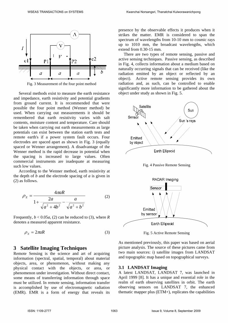
Fig. 3 Measurement of the four point method
Several methods exist to measure the earth resistance and impedance, earth resistivity and potential gradients from ground current. It is recommended that were possible the four point method (Wenner method) be used. When carrying out measurements it should be remembered that earth resistivity varies with salt contents, moisture content and temperature. Care should be taken when carrying out earth measurements as large potentials can exist between the station earth tests and remote earth's if a power system fault occurs. Four electrodes are spaced apart as shown in Fig. 3 (equally spaced or Wenner arrangement). A disadvantage of the Wenner method is the rapid decrease in potential when the spacing is increased to large values. Often commercial instruments are inadequate at measuring such low values. According to the Wenner method, earth resistivity at the depth of b and the electrode spacing of a is given in (2) as follows.
2222 421
4
baa
baa
aRE
+−
++
=πρ (2)
Frequently, b < 0.05a, (2) can be reduced to (3), where R denotes a measured apparent resistance.
aRE πρ 2= (3)
3 Satellite Imaging Techniques Remote Sensing is the science and art of acquiring information (spectral, spatial, temporal) about material objects, area, or phenomenon, without making any physical contact with the objects, or area, or phenomenon under investigation. Without direct contact, some means of transferring information through space must be utilized. In remote sensing, information transfer is accomplished by use of electromagnetic radiation (EMR). EMR is a form of energy that reveals its
presence by the observable effects it produces when it strikes the matter. EMR is considered to span the spectrum of wavelengths from 10-10 mm to cosmic rays up to 1010 mm, the broadcast wavelengths, which extend from 0.30-15 mm. There are two types of remote sensing, passive and active sensing techniques. Passive sensing, as described in Fig. 4, collects information about a medium based on naturally occurring signals that can be received (like the radiation emitted by an object or reflected by an object). Active remote sensing provides its own radiation and, as such, can be controlled to enable significantly more information to be gathered about the object under study as shown in Fig. 5.
Fig. 4 Passive Remote Sensing
Fig. 5 Active Remote Sensing
As mentioned previously, this paper was based on aerial picture analysis. The source of these pictures came from two main sources: i) satellite images from LANDSAT and topographic map based on topographical surveys. 3.1 LANDSAT Imaging A latest LANDSAT, LANDSAT 7, was launched in April 1999 [8]. It has a unique and essential role in the realm of earth observing satellites in orbit. The earth observing sensors on LANDSAT 7, the enhanced thematic mapper plus (ETM+), replicates the capabilities
WSEAS TRANSACTIONS on SYSTEMS Kwanchai Norsangsri, Thanatchai Kulworawanichpong
ISSN: 1109-2777 1063 Issue 9, Volume 8, September 2009

of the thematic mapper instrument on LANDSAT 4 and 5. The ETM+ also includes new features that make it a more versatile and efficient instrument for global change studies, land cover monitoring and assessment and large area mapping. The primary new features on Landsat 7 are: i) a panchromatic band with 15m spatial resolution, ii) on board, full aperture, 5% absolute radiometric calibration and iii) a thermal IR channel with 60m spatial resolution. Fig. 6 showed a satellite image covering Thailand [9]. As mentioned earlier the dot circle is the area of study in this paper. Fig. 7 gave a close view inside the circle of Fig. 2. It revealed city of Nakhon Ratchasima from the space. LANDSAT 7 moves around the earth with near-polar sun-synchronized orbit. It utilizes the 3.8 Giga-bits S-band communication for up- and down-link. X-band is also used for down-link purpose. Its orbital period is 16 days and time to cross the equator is 10 a.m.
Fig. 6 Satellite image covering Thailand [9]
Fig. 7 Satellite image of City of Nakhon Ratchasima [8]
Satellite images acquired from LANDSAT 7 have been exploited. It depends on applications in which specific wavelengths absorbed and/or reflected from targeted materials are involved. Classification of spectral ranges of LANDSAT 7 images is given in Table 4. Fig. 8 shows coverage area of LANDSAT. However, according to applications, size of LANDSAT images is various as shown in Fig. 9. For instance, standard full scene is 183×170 km2 per patch covering a total of 31110 km2. It is also divided into path (P) and row (R) as imaging indices. For Nakhon Ratchasima area, P128 and R49 are codes for a LANDSAT 7 image covering that area. Table 4 Generalized application details of spectral range
Band Number
Spectral Range (microns)
Generalized Application Details
1 0.45 - 0.52 Visible Blue
Coastal water mapping, differentiation of vegetation from soils
2 0.52 - 0.60 Visible Green
Assessment of vegetation vigour
3 0.63 - 0.69 Visible Red
Chlorophyll absorption for vegetation differentiation
4 0.76 - 0.90 Near Infrared
Biomass surveys and delineation of water bodies
5 1.55 - 1.75 Middle Infrared
Vegetation and soil moisture measurements; differentiation between snow and cloud
6 10.4 - 12.5 Thermal Infrared
Thermal mapping, soil moisture studies and plant heat stress measurement
7 2.08 - 2.35 Middle Infrared
Hydrothermal mapping, soil type, mineral
PAN 0.52 - 0.90 Green, Visible Red, Near Infrared
Large area mapping, urban change studies
Nakhon Ratchasima
WSEAS TRANSACTIONS on SYSTEMS Kwanchai Norsangsri, Thanatchai Kulworawanichpong
ISSN: 1109-2777 1064 Issue 9, Volume 8, September 2009

Fig. 8 LANDSAT coverage map
Fig. 9 Scene of satellite
Fig. 10 Path and Row for Thailand
3.2 Classification Techniques In order to obtained information of earth resistivity from the satellite image, two methods of classification are commonly used: unsupervised and supervised classifications [10-11]. In unsupervised classification any individual pixel is compared to each discrete cluster to see which one it is closest to. A map of all pixels in the image, classified as to which cluster each pixel is most likely to belong, is produced (in black and white or more commonly in colors assigned to each cluster). In a supervised classification the interpreter knows beforehand what classes, etc. are present and where each is in one to perhaps many locations within the scene. These are located on the image, areas containing examples of the class are circumscribed (making them training sites), and the statistical analysis is performed on the multiband data for each such class. All pixels in the image lying outside training sites are then compared with the class discriminants derived from the training sites, with each being assigned to the class it is closest to - this makes a map of established classes (with a few pixels usually remaining unknown) which can be reasonably accurate (but some classes present may not have been set up; or some pixels are misclassified. Image classification based on maximum likelihood method is to establish groups of pixels containing similar properties as shown in Fig. 11. With the help from probability principles, any pixel can be classified into a pre-defined group that gives the distribution curve of the group closest to normal distribution. Each pixel containing information acquired from a satellite image must be assigned to be a member of the most likelihood group as described in Fig. 12. From the figure, relationship between spectral information acquired from the satellite image and earth resistivity measured from field test is featured. The weighted distance representing the likelihood can be expressed by the following relation.
)])(()(5.0[
)]ln(5.0[)ln(1
ccT
c
cc
MXCovMX
CovaD
−−
−−=−
(4)
Where D is the weighted distance (likelihood) c is a cluster or group X is a set of measurement vectors cM is a mean vector of a data group ca is probability of a pixel with respect to the group cCov is covariance matrix of a group
cCov is the determinant of cCov
1−cCov = inverse matrix of cCov
WSEAS TRANSACTIONS on SYSTEMS Kwanchai Norsangsri, Thanatchai Kulworawanichpong
ISSN: 1109-2777 1065 Issue 9, Volume 8, September 2009

255
255
Band 3
Band 2
Clay soil
Sand clay mixtureSurface Limestone
Peat Gravel
Fig. 11 Classification Techniques
Fig. 12 Soil resistivity Classification
4 Earth Resistivity Map 4.1 Satellite Image Applications Satellite image data is sent from the satellite to the ground station in a raw digital format, which is essentially a stream of numerical data. The smallest unit of digital data is a bit. A bit is represented by a binary number, which has only two possible values, 0 or 1. A bit can be used to represent any piece of data that has two states, such as on/off, true/false, or open/closed. With only two potential values, a bit does not offer much flexibility in representing data that is more complex than a binary number. Therefore, data is often stored as a collection of eight bits, resulting in a unit of data called a byte. It is important to remember that a satellite image is not just a picture of the target similar to what a simple camera would take. Instead it is a collection of numeric data that is capable of being displayed as an image. The underlying dataset can be manipulated using algorithms (mathematical equations) that correct for errors (like atmospheric interference), re-map the data to a geographical reference point, or extract information that is not readily apparent in the data. The data for two or more images of the same location can even be combined mathematically, creating imagery that is a composite of
multiple datasets. These data products, known as derived products, can be generated by performing calculations on the raw numerical (digital numbers) data. Classification is a process by which a set of items is grouped into classes based on common characteristics. Classification of satellite image data is based on placing pixels with similar values into groups and identifying the common characteristics of the items represented by these pixels. Classification is another tool that is very useful when multispectral imagery of the same geographical region is compared. Algorithms can be used that derive a value for each pixel in the image from its brightness values in each image. Plotting the resulting data on a 2 or 3 dimensional graph can identify clusters of pixels that share common spectral characteristics across multiple bands. This can be summarized in Fig. 13.
Fig. 13 Step of Classification Techniques 4.2 Satellite Imaging Prepared A position on the Earth is referenced in the Universal Transverse Mercator (UTM) coordinate system [12] by the UTM zone, and the easting and northing coordinate pair. Each satellite image must be specified with this coordinate system. Raw satellite data often contain a vast amount of information that is not readily apparent to the analyst. Therefore, image enhancement techniques are used to highlight features of interest and expose subtle differences in the spectral signature of the components of the target. Some of these techniques involve modifying an image in order to improve contrast between features in a well defined spectral range or to improve resolution and detail, while other techniques use complex mathematical calculations to derive an entirely new image from a set of raw image data. False color [13-16] is a technique by which colors are assigned to spectral bands that do not equate to the spectral range of the selected color. This allows an analyst to highlight particular features of interest using a
WSEAS TRANSACTIONS on SYSTEMS Kwanchai Norsangsri, Thanatchai Kulworawanichpong
ISSN: 1109-2777 1066 Issue 9, Volume 8, September 2009
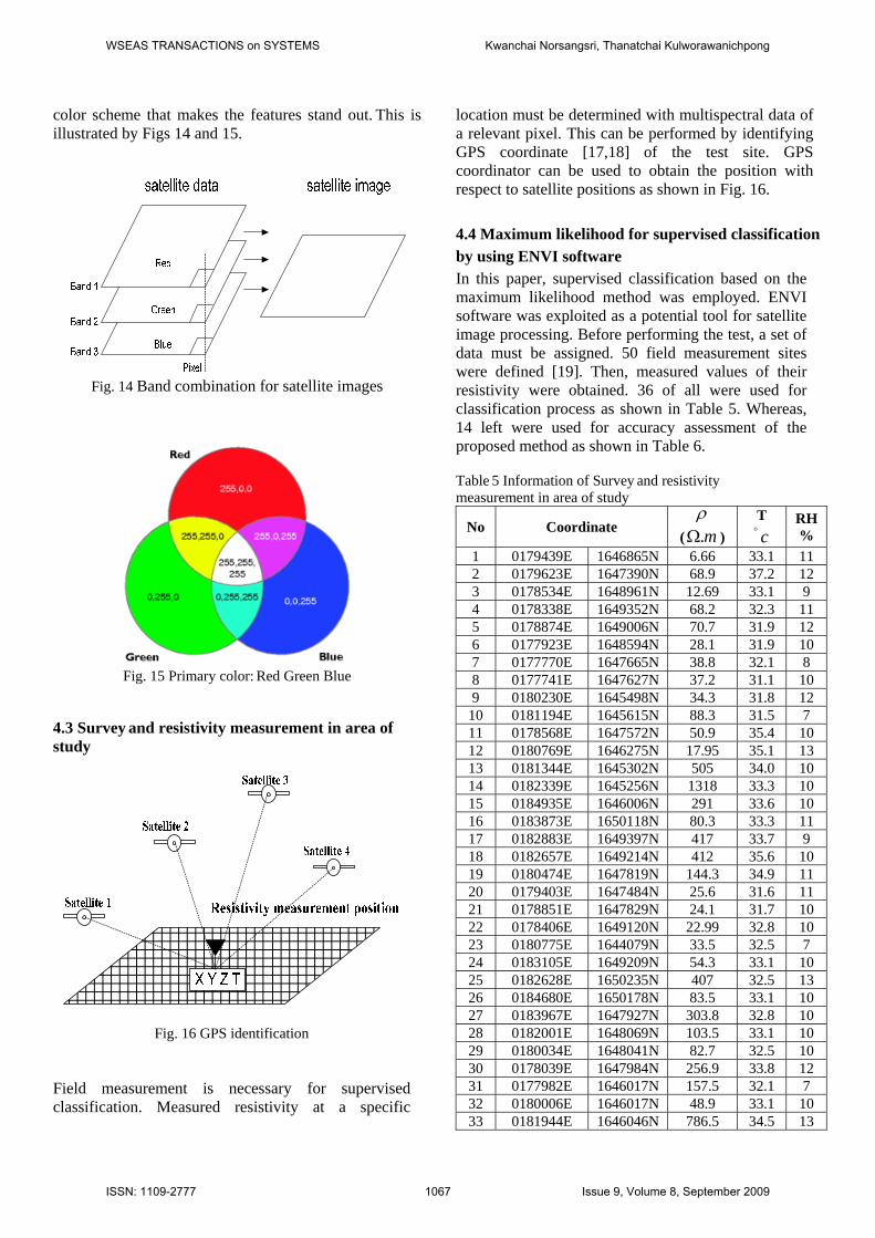
color scheme that makes the features stand out. This is illustrated by Figs 14 and 15.
Fig. 14 Band combination for satellite images
Fig. 15 Primary color: Red Green Blue
4.3 Survey and resistivity measurement in area of study
Fig. 16 GPS identification
Field measurement is necessary for supervised classification. Measured resistivity at a specific
location must be determined with multispectral data of a relevant pixel. This can be performed by identifying GPS coordinate [17,18] of the test site. GPS coordinator can be used to obtain the position with respect to satellite positions as shown in Fig. 16. 4.4 Maximum likelihood for supervised classification by using ENVI software In this paper, supervised classification based on the maximum likelihood method was employed. ENVI software was exploited as a potential tool for satellite image processing. Before performing the test, a set of data must be assigned. 50 field measurement sites were defined [19]. Then, measured values of their resistivity were obtained. 36 of all were used for classification process as shown in Table 5. Whereas, 14 left were used for accuracy assessment of the proposed method as shown in Table 6.
Table 5 Information of Survey and resistivity measurement in area of study
No Coordinate ρ
( m.Ω ) T c°
RH %
1 0179439E 1646865N 6.66 33.1 11 2 0179623E 1647390N 68.9 37.2 12 3 0178534E 1648961N 12.69 33.1 9 4 0178338E 1649352N 68.2 32.3 11 5 0178874E 1649006N 70.7 31.9 12 6 0177923E 1648594N 28.1 31.9 10 7 0177770E 1647665N 38.8 32.1 8 8 0177741E 1647627N 37.2 31.1 10 9 0180230E 1645498N 34.3 31.8 12
10 0181194E 1645615N 88.3 31.5 7 11 0178568E 1647572N 50.9 35.4 10 12 0180769E 1646275N 17.95 35.1 13 13 0181344E 1645302N 505 34.0 10 14 0182339E 1645256N 1318 33.3 10 15 0184935E 1646006N 291 33.6 10 16 0183873E 1650118N 80.3 33.3 11 17 0182883E 1649397N 417 33.7 9 18 0182657E 1649214N 412 35.6 10 19 0180474E 1647819N 144.3 34.9 11 20 0179403E 1647484N 25.6 31.6 11 21 0178851E 1647829N 24.1 31.7 10 22 0178406E 1649120N 22.99 32.8 10 23 0180775E 1644079N 33.5 32.5 7 24 0183105E 1649209N 54.3 33.1 10 25 0182628E 1650235N 407 32.5 13 26 0184680E 1650178N 83.5 33.1 10 27 0183967E 1647927N 303.8 32.8 10 28 0182001E 1648069N 103.5 33.1 10 29 0180034E 1648041N 82.7 32.5 10 30 0178039E 1647984N 256.9 33.8 12 31 0177982E 1646017N 157.5 32.1 7 32 0180006E 1646017N 48.9 33.1 10 33 0181944E 1646046N 786.5 34.5 13
WSEAS TRANSACTIONS on SYSTEMS Kwanchai Norsangsri, Thanatchai Kulworawanichpong
ISSN: 1109-2777 1067 Issue 9, Volume 8, September 2009

34 0183967E 1645989N 324.3 32.4 10 35 0184395E 1646359N 123.7 31.4 11 36 0177583E 1646929N 175.4 32.30 10
Table 6 Information of Survey and resistivity measurement in area of study for Verifying
No Coordinate ρ
( m.Ω ) T c°
RH %
1 0177281E 1647068N 68.8 38.1 10 2 0178314E 1648063N 43.9 34.6 10 3 0178778E 1648388N 8.46 31.9 10 4 0179137E 1648218N 107.2 36.4 10 5 0181507E 1645293N 500 31.9 10
6 0181824E 1648579N 200 33.9 10 7 0184727E 1645344N 311 33.6 10 8 0177868E 1647043N 114.9 32.5 10 9 0181060E 1647442N 256.8 32.1 12
10 0178666E 1645390N 75.5 33.1 7 11 0178353E 1650264N 345.4 32.6 10 12 0184452E 1649067N 32.5 32.7 13 13 0179122E 1648212N 178.1 31.9 10 14 0181288E 1650634N 45.3 31.2 11
5 Results and Discussion This research was conducted by using ENVI software as an image processing tool for extracting earth resistivity from the satellite data. A LANSAT 7 image of a tested area of 50 km2 as shown in Fig. 17 was used for test.
Fig. 17 Satellite image of the test area
A satellite image acquired from LANSAT 7 consists of eight spectral bands with spatial resolutions ranging from 15 – 60 meters. To create earth resistivity map, five mixed bands were prepared for supervised classification as follows.
1. Bands 4-3-2 2. Bands 4-5-3
3. Bands 4-5-7 4. Bands 7-4-3 5. Bands 7-5-3
Table 7 Result of confidence level
Mixed bands Confidence level (%)
4-3-2 64.29
4-5-3 57.14
4-5-7 71.43
7-4-3 71.43
7-5-3 85.71
50 test locations were selected and then measured for earth resistivity. 36 of all were used as input of supervised training process, while 14 left were used for verifying the effectiveness of the earth resistivity classification. Figs 18 – 22 showed visualization of five respective mixed bands as described earlier. Fig. 23-27 presented the earth resistivity map of the test area. This picture was selected from the mixed bands that gave the best estimation of the earth resistivity result. Table 7 gave results of evaluation of confidence level from the supervised classification. The results showed that the mixed bands of 7-5-3 gave the best of 85.71% confidence. The mix of bands 4-5-3 was the worst result of 57.14% confidence.
Fig. 18 Color rendering of the mixed bands 4-3-2
WSEAS TRANSACTIONS on SYSTEMS Kwanchai Norsangsri, Thanatchai Kulworawanichpong
ISSN: 1109-2777 1068 Issue 9, Volume 8, September 2009
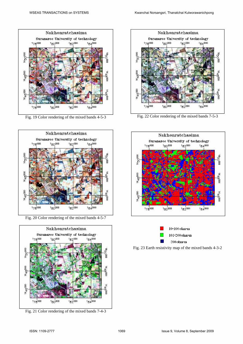
Fig. 19 Color rendering of the mixed bands 4-5-3
Fig. 20 Color rendering of the mixed bands 4-5-7
Fig. 21 Color rendering of the mixed bands 7-4-3
Fig. 22 Color rendering of the mixed bands 7-5-3
Fig. 23 Earth resistivity map of the mixed bands 4-3-2
WSEAS TRANSACTIONS on SYSTEMS Kwanchai Norsangsri, Thanatchai Kulworawanichpong
ISSN: 1109-2777 1069 Issue 9, Volume 8, September 2009

Fig. 24 Earth resistivity map of the mixed bands 4-5-3
Fig. 25 Earth resistivity map of the mixed bands 4-5-7
Fig. 26 Earth resistivity map of the mixed bands 7-4-3
Fig. 27 Earth resistivity map of the mixed bands 7-5-3
6 Conclusion This paper presented a satellite imaging technique of estimating earth resistivity. A 50-km2 satellite image acquired by LANSAT 7 of the test area was used by ENVI program in associative with a set of resistivity data obtained from field measurement in order to evaluate the proposed scheme. By using the maximum
WSEAS TRANSACTIONS on SYSTEMS Kwanchai Norsangsri, Thanatchai Kulworawanichpong
ISSN: 1109-2777 1070 Issue 9, Volume 8, September 2009
likelihood for supervised classification of a mixed band 7, 5 and 3, highest value of 85.71% confidence was obtained. The earth resistivity can be exploited in various fields, for example, power system grounding, lightning, ground fault protection, etc, in both transmission and distribution levels. 7 Acknowledgment The authors would like to acknowledge the financial support of the research grant (E-006-51) sponsored by the Provincial Electric Authority of Thailand, during a period of this work. References: [1] W. Elshorbagy and A. Elhakeem, Risk assessment
maps of oil spill for major desalination plants in the United Arab Emirates, Desalination, Volume 228, Issues 1-3, pp. 200-216, 2008
[2] X. Jin and C. H. Davis, An integrated system for automatic road mapping from high-resolution multi-spectral satellite imagery by information fusion, Information Fusion, Volume 6, Issue 4, pp. 257-273, 2005
[3] G. Finnveden and A. Moberg, Environmental systems analysis tools – an overview, Journal of Cleaner Production, Volume 13, Issue 12, pp. 1165-1173, 2005
[4] Y. Nishigami, H. Sano and T. Kojima,Estimation of forest area near deserts — production of Global Bio-Methanol from solar energy, Applied Energy, Volume 67, Issue 4, pp. 383-393, 2000
[5] G.P. Patil, W.L. Myers, Z. Luo, G.D. Johnson and C. Taillie, Multiscale assessment of landscapes and watersheds with synoptic multivariate spatial data in environmental and ecological statistics, Mathematical and Computer Modelling, Volume 32, Issues 1-2, pp. 257-272, 2000
[6] IEEE Std 142-1991,IEEE Recommended Practice for Grounding of Industrial and Commercial Power Systems, 1993
[7] IEEE, IEEE Guide for Measuring Earth Resistivity Ground Impedance and Earth Surface Potentials of a Ground system, 1983
[8] C. Banman, Supervised and Unsupervised Land Use Classification, spring session 2002
[9] http://maps.google.com/ [10] Tutorials the environment for visualizing images,
ENVI version 3.2, July, 1999 [11] L. Castellana, A. D′Addabbo and G. Pasquariello, A
composed supervised/unsupervised approach to improve change detection from remote sensing,
Pattern Recognition Letters,Volume 28, Issue 4, pp.405-413, 2007
[12] N. G. Terry, Jr., How to read the Universal Transverse Mercator (UTM) Grid, Adapted from GPS World , pp. 32, April, 1996
[13] R.C. Gonzalez and R. E. Wood, Digital image processing, rt3 Edition, 2007
[14] Richards J.A., Remote Sensing Digital Image Analysis, Springer-Verlag, 1994
[15] H. Roosta, R. Farhudi and M.E. Afifi, Comparison between sub-pixel classifications of MODIS images: linear mixture model and neural network model, WSEAS Trans. Environment and Development, Issue 2, Volume 4, pp. 161 – 168, 2009
[16] T. Luemongkol, A. Wannakomol and T. Kulworawanichpong, Rerouting electric power transmission lines by using satellite imagery, WSEAS Trans. Environment and Development, Issue 2, Volume 5, pp. 189 – 198, 2009
[17] R. Bajaj, S. L. Ranaweera, D. P. Agrawal, GPS: Location-Tracking Technology, Computer, vol. 35, no. 4, pp. 92-94, Apr. 2002
[18] V. Barrile, G. Armocida and F. Di Capua, Advanced thermatic mapping: GIS/neureal networks application for tracking isoseismic lines, WSEAS Trans. Environment and Development, Issue 6, Volume 9, pp. 435 – 444, 2009
[19] K. Norsangsri and T. Kulworawanichpong, Application of satellite image processing to earth resistivity map, The 9th WSEAS International Conferences on Power Systems, 3-5 September 2009, Budapest, Hungary, pp. 137 – 141
WSEAS TRANSACTIONS on SYSTEMS Kwanchai Norsangsri, Thanatchai Kulworawanichpong
ISSN: 1109-2777 1071 Issue 9, Volume 8, September 2009