earth observation and remote sensing: why ai is needed?
TRANSCRIPT
Une école de l’IMT
Earth Observation and Remote Sensing:
Why AI is needed?
Master AIC (Apprentissage, Information et Contenu) and D&K (Data & Knowledge) – Université Paris Saclay
Henri Maître - Télécom Paris
October 2020

Une école de l’IMT
Objectives of this course
The objective of this lecture is to give an introduction to the professional
domain of Remote Sensing for engineers and researchers in the fields of
Computer Science, Artificial Intelligence, Image Processing or Pattern
Recognition,
This objective will be reached by several sub-objectives:
• To show how important Remote Sensing is. To show how diverse the application
domains are with a survey of the most important fields of interest: agriculture,
climate, environment survey and monitoring, defense, cartography, land use
planning, …
• To present the scientific context around Earth observation from satellite:
positioning w.r.t. Earth, satellite trajectory, sensor capacities, acquisition rate, etc.
• To inform about the diversity of satellite images: resolution, size, spectral bands,
radiometric accuracy,
14/10/2020 Modèle de présentation Télécom Paris 2

Une école de l’IMT
Objectives of this course (2/2)
This objective will be reached by several sub-objectives (continued)
• To show that Remote Sensing image mining is not the same problem that
image retrieval on the web.
• To present the main characteristics of satellite images which are used for most
of the applications: textures, contours, lines and networks of lines, areas ...
• To enlighten the role of scale and the role of semantics in the context of
satellite image processing,
• To clarify the role of time series
• To show some early results obtained with Machine Learning and handcrafted
primitive classification
• To present the modern approach using deep neural networks
• To show where difficulties and perspectives are.
14/10/2020 Modèle de présentation Télécom Paris 3
Une école de l’IMT
Content
I - Remote Sensing (RS) and RS Images ………………………
• Why remote sensing? …………………………………………..
• Preparing a RS program ……………………………………..
• Image parameters (resolution, spectral bands, repetition).
• Image diversity …………………………….……………………
II- RS Image mining ………………………………………………
• RS archiving problems ………………………………………..
─ RS image mining IS NOT multimedia image mining …..
─ RS image mining specificity …………………………………..
• Hand-crafted features and classification ……………………
─ Expert in the loop, relevance feedback …………………
• Deep Neural Networks ……………………………………….
─ DNN toolbox ……………………………………………….
─ Some instances ……………………………………………
• From Lo to Hi level of semantics ……………………………
3
4
8
14
23
38
39
41
48
58
70
73
76
80
85
4

Une école de l’IMT
Part I - Remote Sensing
and Remote sensing
images
Why? How? For Whom?
5

Une école de l’IMT
Why do we need Remote Sensing
Environnement:
• Meteorology: short-term weather prediction
• Climate: long-term monitoring
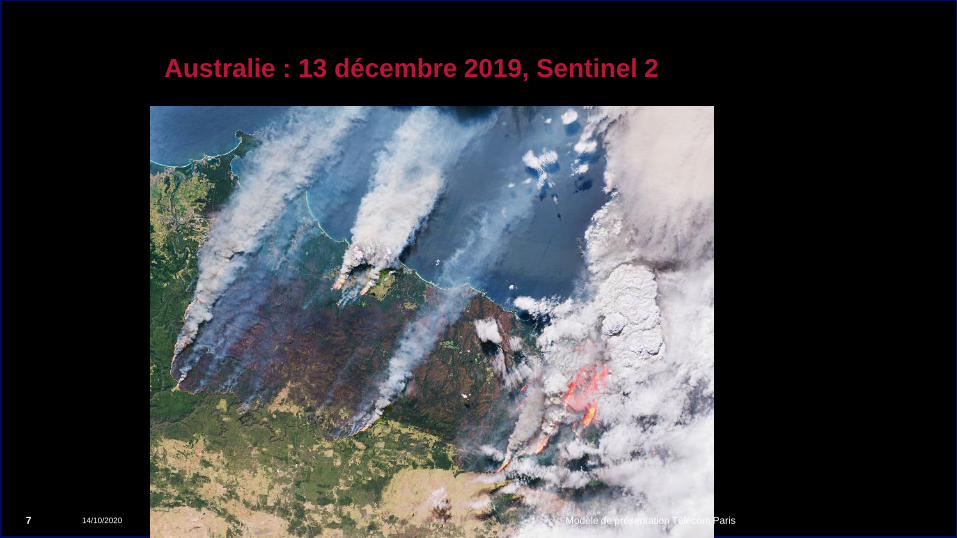
• GMES = Global Monitoring for Environment and Security:
survey of natural and man-made catastrophies
─ volcanos
─ earthquake, tsunamis, floods
─ Industrial hazards
─ Marine pollution
6
Une école de l’IMT
Australie : 13 décembre 2019, Sentinel 2
14/10/2020 Modèle de présentation Télécom Paris 7

Une école de l’IMT
Why do we need Remote Sensing
Agriculture :
• Survey and evaluation of crop & farming production
• Fish & Aquaculture resources management
• Forestry resources planning
• Water management, dams, watering
• Desertification & urban pressure
8

Une école de l’IMT
Why do we need Remote Sensing
Town & country planning:
• Mapping and inventories
• Constructions & public work: railways, airports, harbours,
dams, …
• Cities and Mega-cities management
• Management of moving populations, displacements,
installation
• Climatic impact management
• Crisis management: fires, floods, …
9

Une école de l’IMT
Why do we need Remote Sensing
Defense & Security applications:
• Military deployement preparation
• Military mission debriefing / damage survey
• Intelligence and survey of national/foreign territory
10

Une école de l’IMT
How is prepared a remote sensing
program
11

Une école de l’IMT
Remote sensing mission/program
Where the vocabulary is given: launcher, control station, ground station,
altitude, orbit, geostationary, traveling, revisit time, spectral range,
atmosphere window,
The image parameters: resolution, swath, channel number,
Difference between passive (optical wavelength range) and active (Radar)
sensors
14/10/2020 Modèle de présentation Télécom Paris 12

Une école de l’IMT
How is prepared a remote sensing program
Conceive the sensor: application, customers, scientific and technological
issues, financial issues
Determine which satellite / which launcher
Conceive the ground-station and the data management process :
economical, social and technical issues
15 to 20 years
13

Une école de l’IMT
Telemetry link 1.6 Mbps
S band Station Emiter/Receiver
Telecontrol link 4 kbps
S Band
Customer / using
X Band
Image down link 250 Mbps
X band receiving Station
Data Processing center
Images
Images Request for an image
Acquisition
Programming Operating and
Control Decision Center
Terrestrial links Aerial links S-Band Antenna X Band Antenna
Satellite links with the Earth
S-band : 2 to 4 GHz
X-band : 8 to 12 Ghz
Customer / ordering

Une école de l’IMT
Satellite : orbit choice
Mecanics laws:
• Newton = centripetal force
• Satellite speed = driving force
elliptical or circular trajectory (Kepler)
r
r
r
mF
2
15
r
Earth
12 742
km
Processing
satellite : 800
km Geostationary
36 700 km
Une école de l’IMT
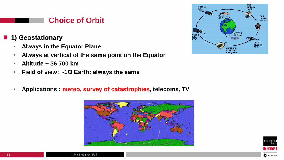
Choice of Orbit
1) Geostationary
• Always in the Equator Plane
• Always at vertical of the same point on the Equator
• Altitude ~ 36 700 km
• Field of view: ~1/3 Earth: always the same
• Applications : meteo, survey of catastrophies, telecoms, TV
16

Une école de l’IMT
Orbit choice
2) Processing satellite (low orbit)
• Altitude ~ 800 km (down to 250 km)
• Circular ~ N/S
• Trajectory : ± polar
• ~ 15 revolutions / day
• Helio-synchronous
17
Une école de l’IMT
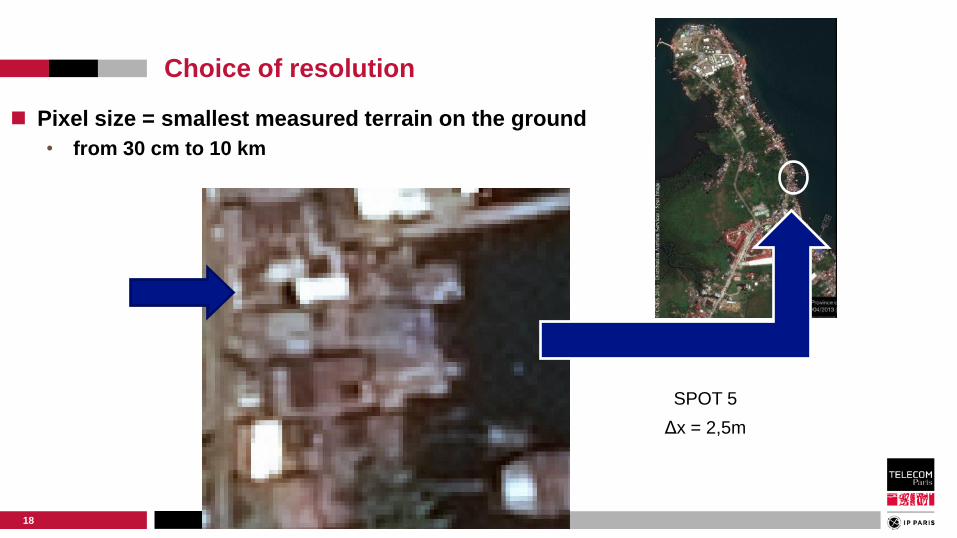
Choice of resolution
Pixel size = smallest measured terrain on the ground
• from 30 cm to 10 km
18
Δx = 2,5m
SPOT 5
Une école de l’IMT
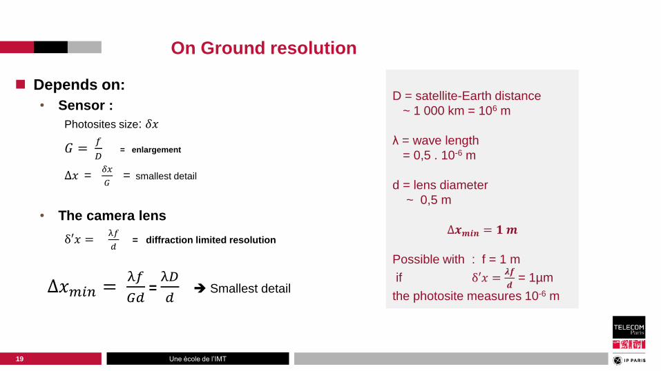
On Ground resolution
Depends on:
• Sensor :
Photosites size: 𝛿𝑥
𝐺 = 𝑓
𝐷 = enlargement
∆𝑥 = 𝛿𝑥
𝐺 = smallest detail
• The camera lens
δ′𝑥 = λ𝑓
𝑑 = diffraction limited resolution
∆𝑥𝑚𝑖𝑛 = λ𝑓
𝐺𝑑 = λ𝐷
𝑑
D = satellite-Earth distance
~ 1 000 km = 106 m
λ = wave length
= 0,5 . 10-6 m
d = lens diameter
~ 0,5 m
∆𝒙𝒎𝒊𝒏 = 𝟏 𝒎
Possible with : f = 1 m
if δ′𝑥 = 𝝀𝒇
𝒅 = 1µm
the photosite measures 10-6 m Smallest detail
19

Une école de l’IMT
Often push-broom sensor
Sensor size along track:
• On line sensor
• = speed x aperture time
In the other direction
• Number of sensors on a line
• from 6 000 to 40 000
Resolution :
• Depends on the lens
20

Une école de l’IMT
Swath choice
Swath = image width
• from 10 km to 10 000 km
• = from 3 000 to 40 000 pixels / line
• Given by the sensor size
• Limited by the communication link with Earth
Revisit delay
15 min for geostationnary sat. (to dump the memory)
• from 1h30 (min) to 1 month for processing satellites
• But … sensor agility!
21
swath

Une école de l’IMT
Video facilities ?
Angle of view ~ + or – 50 degrees:
• MN ~ 2000 km
• 1 rotation around the Earth = 90 min
~ 40 000 km
• Time to go from M to N
= 90*2000/40000 = 4 min 30 s
22
M
N

Une école de l’IMT
Which wavelength?
1 – Passive sensors: measure the energy sent back from Sun by Earth or the
energy radiated by Earth
• Emitted from the Sun (Wien’s law) x Atmosphere transparency x Ground Reflection
• Black and White (Panchromatic)
• Visible = Blue - Green - Red
• Visible and Near Infra-Red : G - R - IR = false colors
• Multispectral : 7 20 channels
• Hyperspectral : 64 512 channels
© Wikipedia © Wikipedia
23

Une école de l’IMT
False colors : NIR-R-G R-G-B
24
vegetation = red
False colors True colors
Une école de l’IMT
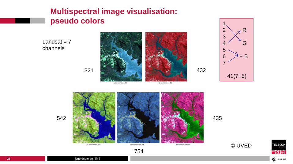
Multispectral image visualisation:
pseudo colors
25
Landsat = 7
channels
© UVED
321 432
754
542 435
1
2 R
3
4 G
5
6 + B
7
41(7+5)

Une école de l’IMT
Which wave length?
2 – Active sensors: EM emitter + receiver
radar = Micro waves: λ= 1 cm to 10 m
• But low resolution ∶ ∆𝑥 = λ𝑓
𝐺𝑑
• With complex processing: SAR = Synthetic Aperture Radar hi resolution
26
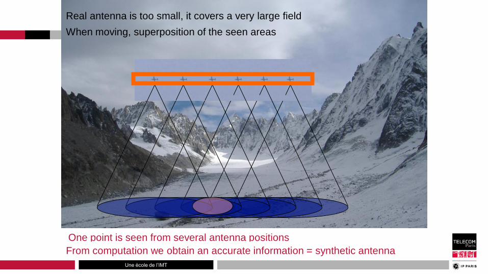
Une école de l’IMT
One point is seen from several antenna positions
When moving, superposition of the seen areas
Real antenna is too small, it covers a very large field
From computation we obtain an accurate information = synthetic antenna

Une école de l’IMT
Satellite images = big data !
Television HD 1 280 x 720 pixels
Television 4k 4 000 x 2 000 pixels
PC display screen 1 600 x 1 200 pixels
Photo camera 5 000 x 4 000 pixels
Spot 1 … 4 6 000 x 6 000 pixels
SPOT 5 24 000 x 24 000 pixels
Quickbird 40 000 x 40 000 pixels
1 600 000 000 pixels = 1,6 Gpixels
= 800 PC display screens
1 SPOT 5 image = 10 s of satellite observation
28
Une école de l’IMT
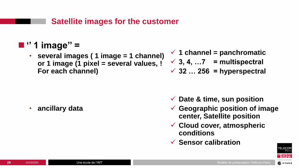
Satellite images for the customer
‘’ 1 image’’ = • several images ( 1 image = 1 channel)
or 1 image (1 pixel = several values, ! For each channel)
• ancillary data
1 channel = panchromatic
3, 4, …7 = multispectral
32 … 256 = hyperspectral
Date & time, sun position
Geographic position of image center, Satellite position
Cloud cover, atmospheric conditions
Sensor calibration
14/10/2020 Modèle de présentation Télécom Paris 29

Une école de l’IMT
Satellite image for the customer
Several levels of processing (de-
pends on the satellite) for instance
• Level 0
• Level 1
• Level 2
• Ortho correction
Raw data as issued from the satellite, on board
geometry (equi angle from the satellite positioning), no
photometric correction, correction of satelite mvt
Registration by projection on the geoid, Equalisation
of sensors,
Accurate registration on a map using a Digital Terrain
Model (DTM), Correction of atmospheric effects
Very accurate registration on a map using a Digital
elevation model (DEM)
14/10/2020 Modèle de présentation Télécom Paris 30

Une école de l’IMT
Image corrections
Radiometric
• Sensor homogeneity or time drift:
─ Calibration on known areas: Nevada,
Atacama, Sahara, Crau)
─ Use of target stars
• Atmospheric corrections
─ Depending or not on meteorological data
─ Taking into account the position of the pixel
in the swath
• Radiometric compensation of
Sun/Satellite angle
─ Using a reflectance terrain model
Geometric corrections
• Roll, pitch and tossing of the satellite
─ Internal consistency of the image
• Projection of the image on the
average altitude geoid
─ Using the X,Y,Z,t positions of the satellite
─ Using Ground control points
• Using a DTM to correct the projection
from the terrain altitude
─ georeferenced images
• Using a DEM to take into account the
man-made constructions
─ Ortho image
14/10/2020 Modèle de présentation Télécom Paris 31

Une école de l’IMT
The role of geometric corrections
14/10/2020 Modèle de présentation Télécom Paris 32
Defects of raw satellite geometry
Use of a DTM to
correct an image

Une école de l’IMT
Coarse vs. fine registration – mosaic presentation
14/10/2020 Modèle de présentation Télécom Paris 33
Worldview-2 image & aerial photography before and after fine registration
Copyright Karantzalos et al.

Une école de l’IMT
Diversity of Remote Sensing Images
34
Une école de l’IMT
Diversity of images
We present several images issued from different satellites with very
different characteristics.
• The main difference comes from resolution and field of view
• Another difference comes from the functional objective of the images:
agriculture, meteorology, defense, land use planning
As a result of technology evolution, the surveyed data change from
clouds, crops, forests to cities and buildings, from highways to
small streets.
14/10/2020 Modèle de présentation Télécom Paris 35

Une école de l’IMT
Meteo satellites: very low resolution
36
Meteosat = 3 km

Une école de l’IMT
Climate/environnement: low resolution
37
INSAT = 2,2 km
Une école de l’IMT
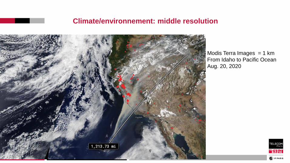
Climate/environnement: middle resolution
38
Modis Terra Images = 1 km
From Idaho to Pacific Ocean
Aug. 20, 2020
Une école de l’IMT
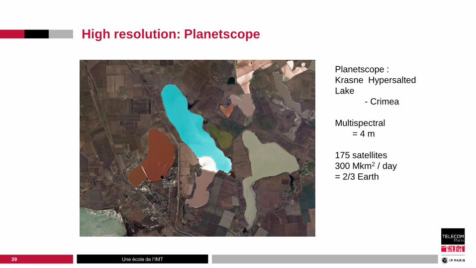
High resolution: Planetscope
39
Planetscope :
Krasne Hypersalted
Lake
- Crimea
Multispectral
= 4 m
175 satellites
300 Mkm2 / day
= 2/3 Earth

Une école de l’IMT
SPOT 5 : high resolution ; pixel = 2,5 m
40

Une école de l’IMT
Very high resolution
41
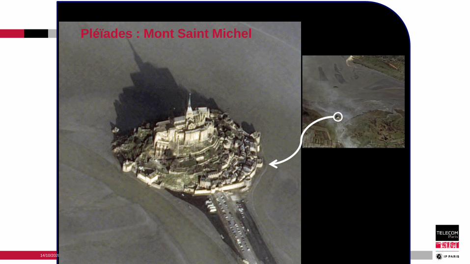
Pléïades :
Bora-Bora
Panchro
= 0,70 m
Multispectral
= 2, 8 m

Une école de l’IMT
Very high resolution: Quickbird
42
Panchro
= 0,61 m
Multispectral
= 2, 4 m
Une école de l’IMT 14/10/2020
Pléïades : Mont Saint Michel

Une école de l’IMT
Auckland New-Zealands
44
Une école de l’IMT
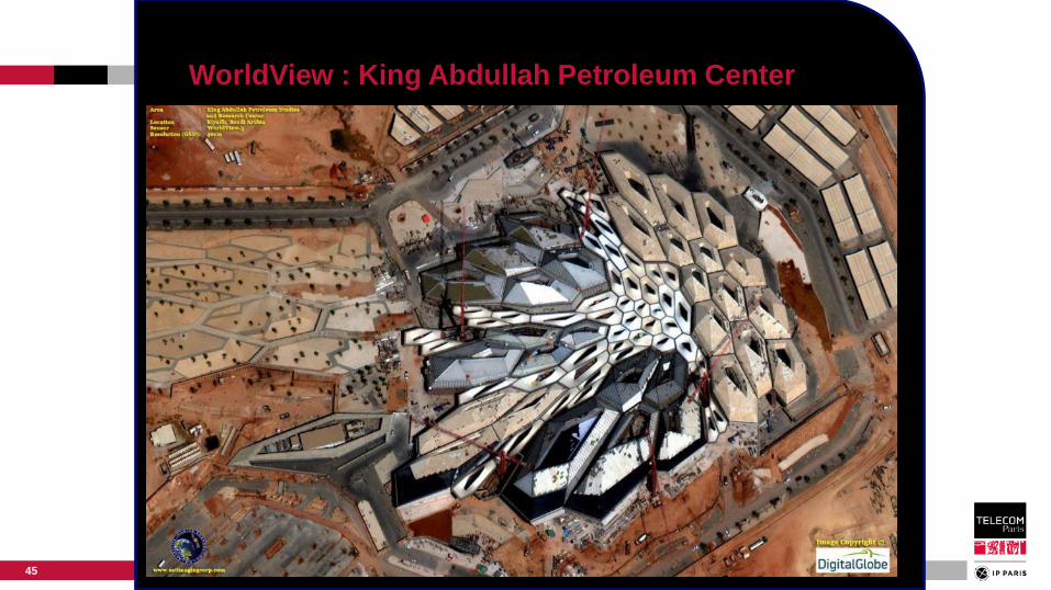
WorldView : King Abdullah Petroleum Center
45

Une école de l’IMT 46
Ikonos – Lebanon: agriculture

Une école de l’IMT
WorldView : Bayan Mines (China)
47
Une école de l’IMT
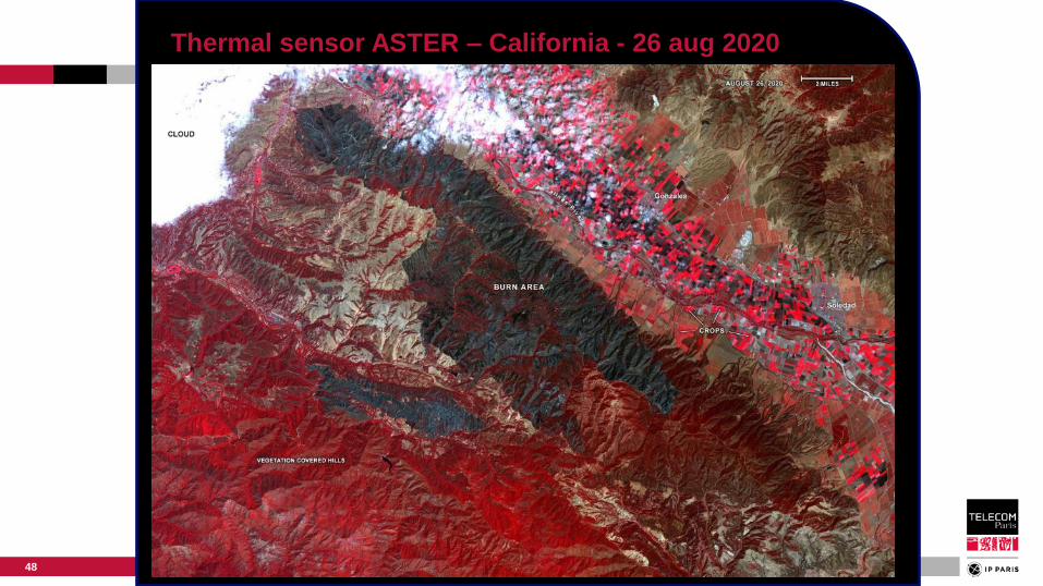
Thermal sensor ASTER – California - 26 aug 2020
48

Une école de l’IMT 14/10/2020 49
1976
2009
49
Temporal evolution: Baikal Lake
with SPOT
Une école de l’IMT
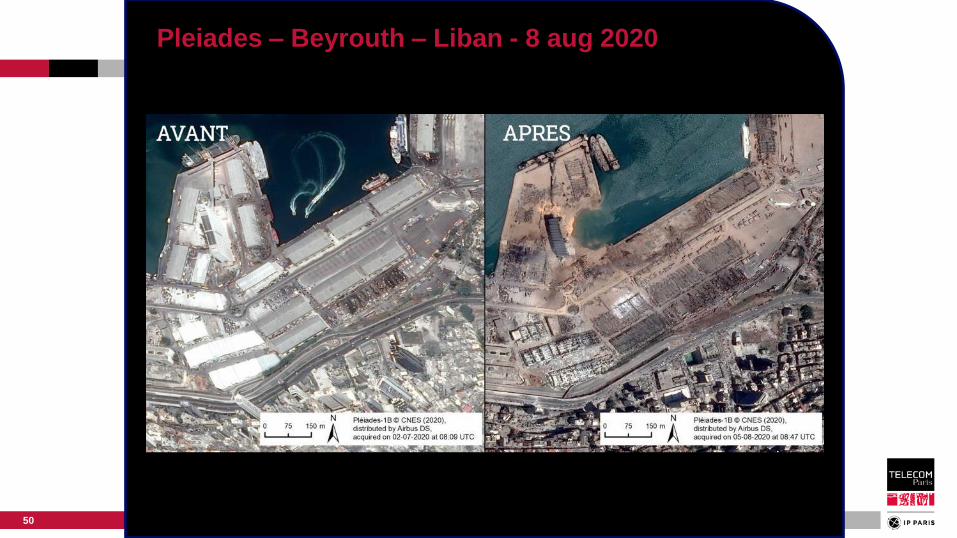
Pleiades – Beyrouth – Liban - 8 aug 2020
50

Une école de l’IMT
Part II – Remote Sensing
Image Mining
51

Une école de l’IMT
Remote Sensing Imaging: Archiving
Problems and Issues
52

Une école de l’IMT
Remote sensing imaging IS big data
Hundreds of satellites, each with tenth of thousands of images, each with tenth
of millions of pixels
A huge problem … storage of data refreshing storage subject to technological
evolutions: tapes, discs, VLSI
Additional problem: where is information?
Solution: Image mining
• Has been developed since about 2000, firstly with classification of handmade
features, then more successfully with deep neural networks (DNN)
• DNN are end-to-end solutions Blind techniques, not yet ‘’explainable’’ . They are
still under development and far from being stabilized for remote sensing applications.
• Handmade features are much more ‘’explainable’’, they are well adapted to man
machine interaction and human supervision. We will spend more time with them
14/10/2020 Modèle de présentation Télécom Paris 53

Une école de l’IMT Page 54
Satellite Image archives
How can we store millions of images?
How can we ensure durability of storage?
How knowing that information exists?
How retrieving information?
How exploiting information?
Data Mining directly on image files
When searching in a small set of images
Indexing images when received
data mining on index
When searching in large sets
Not treated here

Une école de l’IMT
RS Image mining IS NOT MultiMedia
Image Mining
55

Une école de l’IMT
Multimedia vs. Satellite
Image retrieval on the web (Google-like) is very efficient and most
used. Is it possible to use it for satellite images?
Efficient techniques for image retrieval on the web (called here
‘’Multimedia images’’) are based on semantic descriptors attached
to the image. These descriptors do not exist for satellite images.
Multimedia image retrieval looks for ‘’exact’’ retrieval. Satellite
image retrieval looks for ‘’similar configurations’’. specific
techniques with specific metrics have to be developed.
14/10/2020 Modèle de présentation Télécom Paris 56
Une école de l’IMT
Mining in Multimedia Image databases
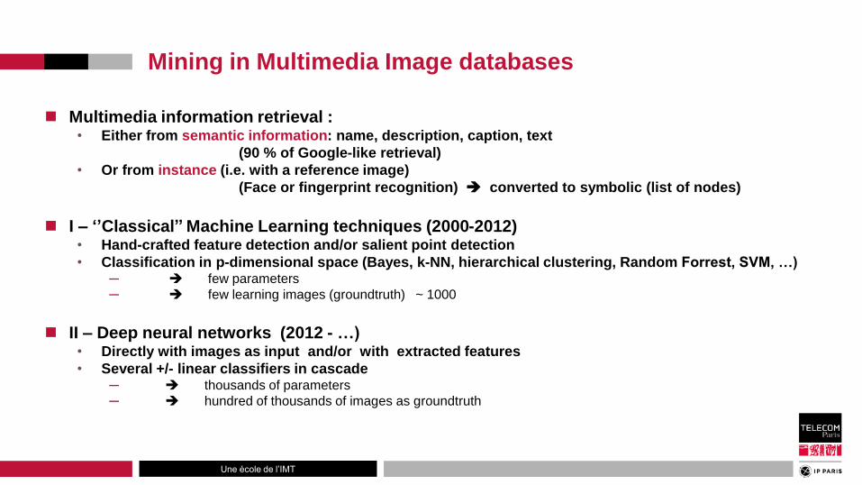
Multimedia information retrieval : • Either from semantic information: name, description, caption, text
(90 % of Google-like retrieval)
• Or from instance (i.e. with a reference image)
(Face or fingerprint recognition) converted to symbolic (list of nodes)
I – ‘’Classical’’ Machine Learning techniques (2000-2012) • Hand-crafted feature detection and/or salient point detection
• Classification in p-dimensional space (Bayes, k-NN, hierarchical clustering, Random Forrest, SVM, …) ─ few parameters
─ few learning images (groundtruth) ~ 1000
II – Deep neural networks (2012 - …) • Directly with images as input and/or with extracted features
• Several +/- linear classifiers in cascade ─ thousands of parameters
─ hundred of thousands of images as groundtruth

Une école de l’IMT
Multimedia image mining: handcrafted features + classification
Multimedia information retrieval from instances:
• Choices: to be robust wrt possible differences
─ scale, lighting, orientation, color, … invariance
• Strategy: detect invariant features
─ Histograms, color distribution, area-based segmentation, graph description, …
─ Textures
─ Salient point detection: Harris, SIFT, SURF, …
• Represent the image as a vector in a p dimensional space ℝp
• Classification : Bayès, k-NN, dynamic clustering, SVM (Support Vector
Machine), Graph-tree, random forrest…

Une école de l’IMT
Salient points: SIFT

Une école de l’IMT
Specificities of RS Image mining
63

Une école de l’IMT Page 64
Category-based retrieval in specific data-bases
Mostly attached to specific domains:
• Biomedical
• Biology
• Astronomy
• Remote sensing and satellite images
Goal: to retrieve images « looking the same » as a given sample in very specialized data-bases
Different from : retrieving the exact object in a very broad data-base
Une école de l’IMT Page 65
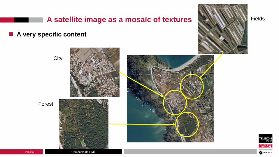
A satellite image as a mosaïc of textures
A very specific content
Fields
City
Forest

Une école de l’IMT
But … a same region may provide different images
66
From : Tong et al.
arXiv 1807.05713 - 2018
Meteorological variations
Seasonnal agricultural variations

Une école de l’IMT
The role of scale
67
High-Badakchan, Tadjikistan - Ikonos
15 m 1 m

Une école de l’IMT
Main scales
< 1 meter = Very high resolution : fine details in urban context, roofs,
chemneys, cars, pedestrians, zebra crossings, containers, fences, small
boats, … Ikonos, Pleiades, QuickView
1 m < … < 5 m = High resolution : urban structures, houses, streets,
gardens, individual trees, railway & road networks, … SPOT 5
5 m < … < 30 m = Middle resolution: fine landcover, coarse urban structure:
dense urban, residential or commercial areas, Landsat, Spot 1-3
> 30 m = low resolution: global landcover
68
Une école de l’IMT
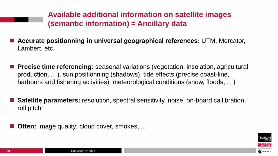
Available additional information on satellite images
(semantic information) = Ancillary data
Accurate positionning in universal geographical references: UTM, Mercator,
Lambert, etc.
Precise time referencing: seasonal variations (vegetation, insolation, agricultural
production, …), sun positionning (shadows), tide effects (precise coast-line,
harbours and fishering activities), meteorological conditions (snow, floods, …)
Satellite parameters: resolution, spectral sensitivity, noise, on-board callibration,
roll pitch
Often: Image quality: cloud cover, smokes, …
69

Une école de l’IMT
Satellite image indexing is difficult
What are we looking for? It is not clear! (image production and image use are 2 different jobs)
• Precise objects: ─ Boat Road-crossing Troops movements
─ Building Airplane landing area
• Generic objects: ─ Marina Forest fire
─ Greenhouse cultures refugee camps
─ Oil pipeline typhoon hazards
─ Geological synclinal
• Specific terrain configurations: ─ Conducive to: … floods, … desertification, … urban pollution, …
─ Conducive to: … build a factory, … plan a bombing, … cultivate marijuana
Une école de l’IMT Page 71
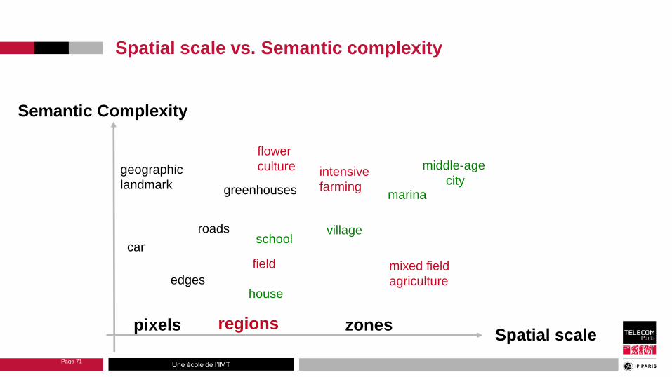
Spatial scale vs. Semantic complexity
pixels regions zones Spatial scale
Semantic Complexity
edges
roads
field
intensive
farming
house
village
middle-age
city
school
flower
culture
car
geographic
landmark
mixed field
agriculture
greenhouses marina

Une école de l’IMT
Hierarchical representation
spectral properties (R,G,B,IR)
Pixel contrast / texture
edges, contours
Objects Scene
form / shape
Region
content (spectral : textural)
72
Increasing semantics
warehouse
wharf
sea
house
network
fields

Une école de l’IMT
RS image processing & hand-crafted
feature detection
73

Une école de l’IMT
Handcrafted features
Handcrafted features are chosen by the user to reflect what is known about
the object under investigation.
• It may be positive: reflecting a property which is strongly associated with the
looked for object
─ (for instance swimming pools in residential areas)
• It may be negative if we know that its presence is not possible in the looked for
object
─ (for instance gas cisterns in residential areas)
Handcrafted features are issued from application expertise
Handcrafted features are detected using image processing expertise
14/10/2020 Modèle de présentation Télécom Paris 74

Une école de l’IMT
Mining in RS Image databases
Semantic information retrieval : • From ancillary data
I – Classical Machine Learning techniques (2000-2012) • Image Processing
• Hand-crafted feature detection and/or salient point detection
• Classification in p-dimensional space
─ few parameters
─ few learning images (groundtruth) ~ 1000
II – Deep neural networks (2012 - …) • Directly with images as input and/or with extracted features
• Several +/- linear classifiers in cascade
─ thousands of parameters
─ hundred of thousands of images as groundtruth

Une école de l’IMT Page 76
Probabilistic evaluation
p(Li|w)

Une école de l’IMT Page 77
Hand crafted features
Radiometry • Multispectral : channels
• Specific combinations for remote sensing : NDVI (= 𝑵𝑰𝑹−𝒓𝒆𝒅
𝑵𝑰𝑹+𝒓𝒆𝒅) , IB , ISU
Textures • Gabor Filters
• Haralick cooccurrence matrices and their descriptors
• Quadratic Mirror Filters (wavelets)
• Contourlet decomposition
• Steerable wavelets
• Markov random fields parameters (Gaussian, Laplacian, Log-laplacian …)
Structures • Contours & edges (coastline, deserts, …), regions (lakes, forests, …)
• Objects : roads, buildings, rivers, lakes
• Roads, Railways or River networks

Une école de l’IMT Page 78
Some efficient choices
Indexing: small subimages: (~ 64 x 64 pixels) = 320 m x 320 m on the ground for SPOT 5 images
Mixed features:
• Radiometry (Panchro only)
• Structure (contours)
• wavelets : 2 directions, 4 scales
Automatic feature selection (supervised: ReliefF, Fisher FS, SVM-RFE or unsupervised: MIC
(Max Information Compression), k-means FS)
~ 100 features with or 10 to 20 features
redundancy without redundancy
Give names to classes (from label to name)
• Waste fields
• Cultures
• Housing
• Road and river networks

Une école de l’IMT Page 79
Classification
label = 24
or
name = « Corn field »
Semantic labelling
Many different classifiers:
• MAP & Bayes decision
• K-nearest neigbours
• Graph tree, Random Forest
• Kernel methods (SVM = Support Vector Machine)
• Hierarchical clustering
Supervised
or
Unsupervised
Partial volume effect
Une école de l’IMT Page 80
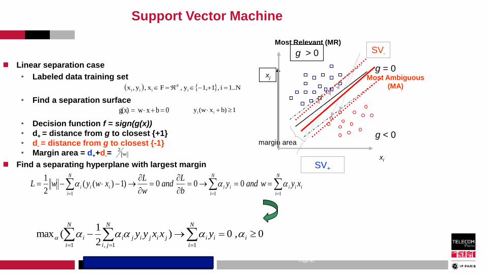
Support Vector Machine
Linear separation case
• Labeled data training set
• Find a separation surface
• Decision function f = sign(g(x))
• d+ = distance from g to closest {+1}
• d- = distance from g to closest {-1}
• Margin area = d++d-=
Find a separating hyperplane with largest margin
0bx w g(x)
xi
xj
g > 0
g < 0
g = 0
1..Ni , 11,y , F x, y,x i
d
iii
w2
margin area
SV+
SV-
1b)x(wy ii
N
i
N
i
N
i
iiiiiiii xywandyb
Land
w
LxwywL
1 1 1
000)1)((2
1
0,0)2
1(max
11,1
i
N
i
ii
N
ji
jijiji
N
i
i yxxyy
Most Relevant (MR)
Most Ambiguous
(MA)
Une école de l’IMT Page 81
How to introduce semantics?
Where are words coming from?
Supervised methods • Fully manual indexing (experts or crowd sourcing)
• Partly: learning (relevance feedback)
Contextual analysis of the document • Tittle, caption, text, web site
Use of external data-bases • Corine Land Cover (to learn classes and categories)
• Maps and GIS (annotation)
Semantics inference • Bayesian Modelling
• Latent Models = Dirichlet, Blei & Jordan
• « Ontological » deduction
• Spatial reasonning

Une école de l’IMT Page 82
Example : CorineLandCover ontology
111: Continuous urban fabric
112: Discontinuous urban fabric
121: Industrial or commercial units
122: Road and rail networks and associated land
…
211: Non-irrigated arable land
221: Vineyards
222: Fruit trees and berry plantations
…
231: Pastures
242: Complex cultivation patterns
243: Land principally occupied by agriculture with significant areas of natural vegetation
311: Broad-leaved forests
312: Coniferous forests
313: Mixed forests
…
411: Inland marshes
…
511: Water courses
…

Une école de l’IMT
Page 83
Supervised classes
Residential
areas
Planes
Industrial
tanks & cisterns
Railway
marshalling yard

Une école de l’IMT Page 84
Supervised classes
factories
Dense urban
area
villages
Urban parks

Une école de l’IMT Page 85
Supervised classes
Graveyards
Road
interchange
Castle
parks
Parking lots

Une école de l’IMT
How to express results?
Classification rate 97.3 % (or error rate: 2.7 %)
Confusion matrix
Receiver Operating Characteristic (ROC Curve)
Convert TP and FP into FPR and TPR ϵ [0,1]
Plot TPR = f(FPR) for many different parameters
Without specific instruction, take the closest
point from A = (0,1) as working condition
86
Present object Absent object
Positive detection True positive (TP) False positive (FP)
(type I error)
Negative detection False negative
(type II error) True Negative
TPR
sensitivity
FPR
O O
1
1
A
Une école de l’IMT Page 87
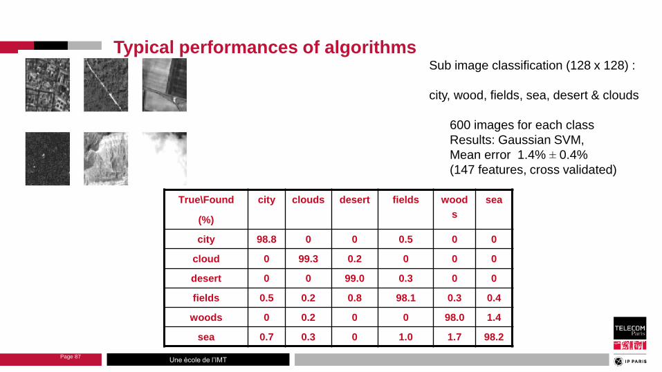
Sub image classification (128 x 128) :
city, wood, fields, sea, desert & clouds
600 images for each class
Results: Gaussian SVM,
Mean error 1.4% ± 0.4%
(147 features, cross validated)
True\Found
(%)
city clouds desert fields wood
s
sea
city 98.8 0 0 0.5 0 0
cloud 0 99.3 0.2 0 0 0
desert 0 0 99.0 0.3 0 0
fields 0.5 0.2 0.8 98.1 0.3 0.4
woods 0 0.2 0 0 98.0 1.4
sea 0.7 0.3 0 1.0 1.7 98.2
Typical performances of algorithms

Une école de l’IMT Page 88 ENS-Ker
Lann - 3-04-2007
How many features?
Automatic feature selection
• Wrappers
• Filters (mutual information)
• Embedded (Lasso)
Une école de l’IMT
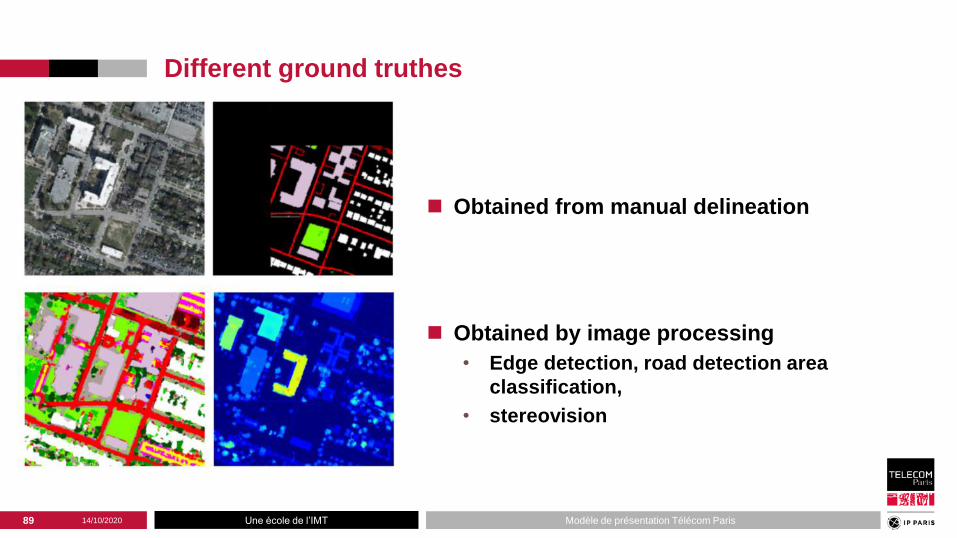
Different ground truthes
Obtained from manual delineation
Obtained by image processing
• Edge detection, road detection area
classification,
• stereovision
14/10/2020 Modèle de présentation Télécom Paris 89

Une école de l’IMT
Using a human expert to improve
learning
« A man (woman ?) in the loop »
Une école de l’IMT Page 91
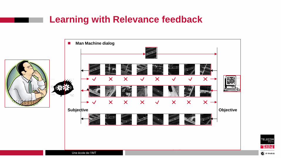
Learning with Relevance feedback
Man Machine dialog
Subjective Objective
Une école de l’IMT Page 92
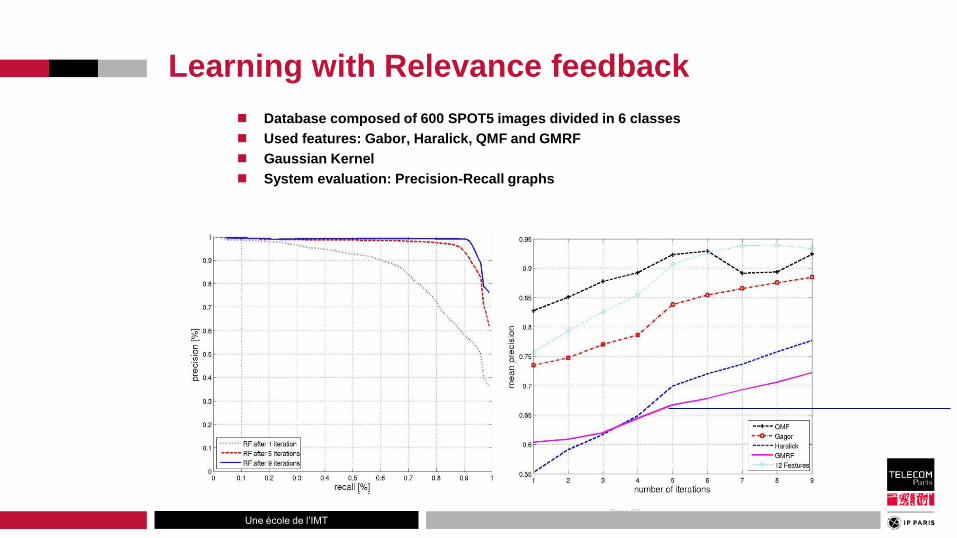
Database composed of 600 SPOT5 images divided in 6 classes
Used features: Gabor, Haralick, QMF and GMRF
Gaussian Kernel
System evaluation: Precision-Recall graphs
Learning with Relevance feedback

Une école de l’IMT
Deep Neural Networks
93

Une école de l’IMT
Deep Neural Networks
As for many other Pattern Recognition problems, DNN is one of the most
efficient solution for Remote Sensing applications.
Solutions take benefit of the development of efficient architectures in the field
of Pattern Recognition
Softwares and Architectures are not yet stabilized and are still under
investigations
Domain application expertise is required to build the annotated ground data
set.
14/10/2020 Modèle de présentation Télécom Paris 94
Une école de l’IMT
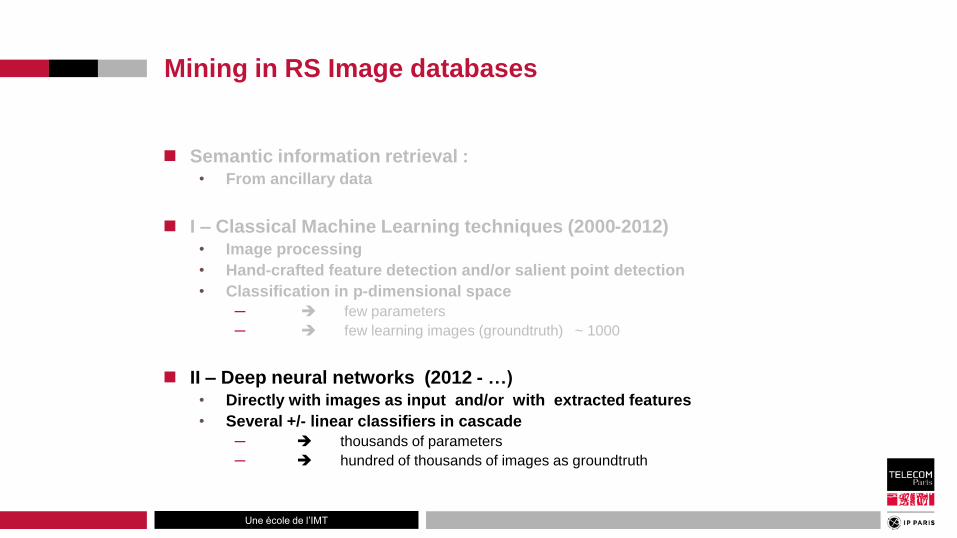
Mining in RS Image databases
Semantic information retrieval : • From ancillary data
I – Classical Machine Learning techniques (2000-2012) • Image processing
• Hand-crafted feature detection and/or salient point detection
• Classification in p-dimensional space
─ few parameters
─ few learning images (groundtruth) ~ 1000
II – Deep neural networks (2012 - …) • Directly with images as input and/or with extracted features
• Several +/- linear classifiers in cascade
─ thousands of parameters
─ hundred of thousands of images as groundtruth

Une école de l’IMT
Some references (dated 01/10/2020)
Maxwell, A. E., Warner, T. A., & Fang, F. (2018). Implementation of machine-learning classification in remote sensing: An applied review. International Journal of Remote Sensing, 39(9), 2784-2817.
Holloway, J., & Mengersen, K. (2018). Statistical machine learning methods and remote sensing for sustainable development goals: a review. Remote Sensing, 10(9), 1365.
Carter, C., & Liang, S. (2019). Evaluation of ten machine learning methods for estimating terrestrial evapotranspiration from remote sensing. International Journal of Applied Earth Observation and Geoinformation, 78, 86-92
Li, J., Huang, X., & Gong, J. (2019). Deep neural network for remote-sensing image interpretation: Status and perspectives. National Science Review, 6(6), 1082-1086.
Ghorbanzadeh, O., Blaschke, T., Gholamnia, K., Meena, S. R., Tiede, D., & Aryal, J. (2019). Evaluation of different machine learning methods and deep-learning convolutional neural networks for landslide detection. Remote Sensing, 11(2), 196.
Yuan, Q., Shen, H., Li, T., Li, Z., Li, S., Jiang, Y., ... & Gao, J. (2020). Deep learning in environmental remote sensing: Achievements and challenges. Remote Sensing of Environment, 241, 111716.
Zhang, L., Zhang, L., & Du, B. (2016). Deep learning for remote sensing data: A technical tutorial on the state of the art. IEEE Geoscience and Remote Sensing Magazine, 4(2), 22-40.
Maggiori, E., Tarabalka, Y., Charpiat, G., & Alliez, P. (2017). Convolutional neural networks for large-scale remote-sensing image classification. IEEE Transactions on Geoscience and Remote Sensing, 55(2), 645-657. Tong, X. Y., Lu, Q., Xia, G. S., & Zhang, L. (2018). Large-scale Land Cover Classification in GaoFen-2 Satellite Imagery. arXiv preprint arXiv:1806.00901.
Boualleg, Y., & Farah, M. (2018, July). Enhanced Interactive Remote Sensing Image Retrieval with Scene Classification Convolutional Neural Networks Model. In IGARSS 2018-2018 IEEE International Geoscience and Remote Sensing Symposium (pp. 4748-4751). IEEE.
Marmanis, D., Datcu, M., Esch, T., & Stilla, U. (2016). Deep learning earth observation classification using ImageNet pretrained networks. IEEE Geoscience and Remote Sensing Letters, 13(1), 105-109.
Kussul, N., Lavreniuk, M., Skakun, S., & Shelestov, A. (2017). Deep learning classification of land cover and crop types using remote sensing data. IEEE Geoscience and Remote Sensing Letters, 14(5), 778-782.
Penatti, O. A., Nogueira, K., & dos Santos, J. A. (2015). Do deep features generalize from everyday objects to remote sensing and aerial scenes domains?. In Proceedings of the IEEE conference on computer vision and pattern recognition workshops (pp. 44-51).
Pelletier, C., Webb, G. I., & Petitjean, F. (2019). Temporal convolutional neural network for the classification of satellite image time series. Remote Sensing, 11(5), 523.
Zhang, S., He, G., Chen, H. B., Jing, N., & Wang, Q. (2019). Scale adaptive proposal network for object detection in remote sensing images. IEEE Geoscience and Remote Sensing Letters, 16(6), 864-868.
96

Une école de l’IMT
Deep Neural Network
97
From: I. Bloch, AIC
? ?
Which input?
Raw image
Processed image (filtered, segmented …)
Feature detected image (classified, edge detected, …)
Features
Which output?
Densely classified image
Detected targets
List of targets
List of Features
Which architecture? • # layers,
• type of layers
Which protocole? • Feature learning
• Fine tuning

Une école de l’IMT
CNN basic components
98
Convolutional layer: with rxr kernel – down scaling
Nonlinearity: sigmoïd or RELU (rectified linear unit)
Pooling layer: single value taken from
a set of values - ex: max on a rxr patch
Autoencoder: symetrical NN to reduce the model dimensionality

Une école de l’IMT
CNN basic components
99
Fully convolutional layer: to perform a large distance context dependance
Transfer coding: to learn from a database and use for another one
Fine Tuning: to specify a network to a given task after training on a general
purpose data base
Yoyo architecture : downsampling for feature extraction then upsampling
for fine positioning of targets

Une école de l’IMT
Most used components for RS-CNN (2019)
CNN from the Pattern Recognition community • AlexNet
• GoogleNet
• VGGNet
• ResNet
• Inception
Training sets (specific or not to Remote Sensing community) • ImageNet (General purpose image library for pattern recognition)
• UC Merced DataSet (Aerial images / 21 classes)
• OSM - OpenStreetMap (Aerial Image Database)
• Google Street Map (hi level semantic)
• NLCD - USGS data Base (Geological survey)
• Corinne Landcover (Agriculture & vegetation)
• Gaofen Image Dataset (GID) (Hi Resolution Satellite)
• …
100

Une école de l’IMT
Instance # 1 : Basic CNN (DLR)
With UC Merced Land database (aerial / 21 classes)
With pre-trained CNN (Imagenet)
Fine-tuned full convolutional layers with enhanced data
101
Marmanis et al. IEEE TGRS, Jan 2016

Une école de l’IMT
Instance # 2 : fully CNN (Inria)
102
Patch-based CNN Fully convolutional Patch -based CNN
Image ground truth patch based fully convolutional SVM
Maggiori et al. IEEE TGRS, feb 2017
Detection of buildings

Une école de l’IMT
Instance # 3 : RS CNN (Liemars/Wuhan)
103
Tong et al. arXiv 1807.05713 - 2018
Pretrained with ResNet

Une école de l’IMT
Instance # 3 : RS CNN (Liemars/Wuhan)
104
From : Tong et al.
arXiv 1807.05713 - 2018
Cooperation between classifying (sparse) and segmenting (dense)
Tong et al. arXiv 1807.05713 - 2018

Une école de l’IMT
Instance # 3 : RS CNN (Liemars/Wuhan)
105
Tong et al. arXiv 1807.05713 - 2018

Une école de l’IMT
From Low to High Level - Changing the scale

Une école de l’IMT
Complexity of images
107
Analysis window : real size
128 x 128 pixels
Analysis window : enlarged

Une école de l’IMT
Scale enlargement strategy
108
Pyramid
Sliding window
Growing and Merging

Une école de l’IMT Page 109
Hierarchical representation
pixels regions zones
Spatial scale
Semantic Complexity
edges
roads
field
Intensive farming
house
village
Middle-age city
school
Flower culture
car
Geographic landmark
Mixed field agriculture
greenhouses
Marina
Two goals:
• Enlarge the field of view
• Increase the semantic level
Grouping strategy:
• Sliding window
• Pyramid
• Growing and Merging
Decision strategy:
• Bag of Visual Words (BOVW)
Une école de l’IMT
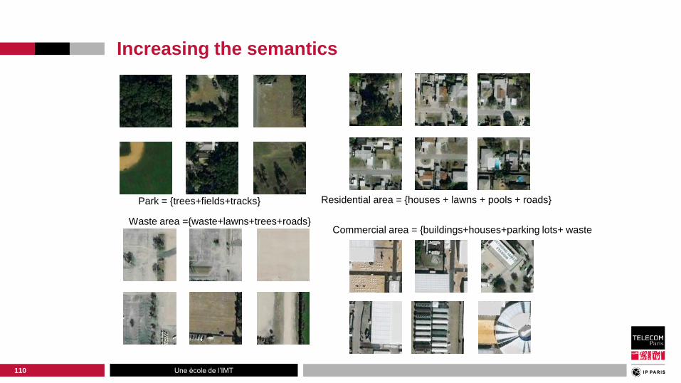
Increasing the semantics
110
Park = {trees+fields+tracks}
Waste area ={waste+lawns+trees+roads}
Residential area = {houses + lawns + pools + roads}
Commercial area = {buildings+houses+parking lots+ waste

Une école de l’IMT Page 111
Probabilistic evaluation
p(Li|w)

Une école de l’IMT
Decision making: Bag of Words
2 levels H=high (unknown) L = low (known)
List of N classes at H = {c1,c2,… cN}
At H : 1 super-region with n objects, each ∈ 1 class = n labels described by the ordered list of the probability (or the occurrence) of each class:
Rk={p1,p2, …pn}
Classify H according to the Rk
• Naïve Bayes : 𝒄∗= argmax 𝒑 𝒄 𝒙 = argmax 𝒑 𝒄 𝒑 𝒙𝒌 𝒄
𝒏𝒌=𝟏
• Improving Naïve Bayes:
─ pLSA = Probabilistic Latent Semantic Analysis
─ LDA = Latent Dirichlet Analysis
112