each as - nasa · felt that understanding classification in these broad cat- egories was necessary...

DRAFT VERSION FEBRUARY 13, 2004 Preprint typeset using I4TFJ style emulateapj v. 10/10/03

AUTOMATED CLASSIFICATION OF ROSAT SOURCES USING HETEROGENEOUS MULTIWAVELENGTH SOURCE CATALOGS

T. A. MCGLYNN', A. A. SUCHKOV', E. L. WINTER': R. J. HANISCH2, R. L. WHITE', F. OCHSENBEIN3, S. DERRIERE3, W. VOWS4, & M. F. CORCORAN'

Draft version February 19, ZOO4

ABSTRACT We describe an on-line system for automated classification of X-ray sources, ClassX, and present preliminary results of classification of the three major catalogs of ROSAT sources, RASS BSC, RASS FSC, and WGACAT, into six class categories: stars, white dwarfs, X-ray binaries, galaxies, AGNs, and clusters of galaxies. ClassX is based on a machine learning technology. It represents a system of classifiers, each classifier consisting of a considerable number of oblique decision trees. These trees are built as the classifier is 'trained' to recognize various classes of objects using a training sample of sources of known object types. Each source is characterized by a preselected set of parameters, or attributes; the same set is then used as the classifier conducts classification of sources of unknown identity. The ClassX pipeline features an automatic search for X-ray source counterparts among heterogeneous data sets in on-line data archives using Virtual Observatory protocols; i t retrieves from those archives all the attributes required by the selected classifier and inputs them to the classifier. The user input to ClassX is typically a file with target coordinates, optionally complemented with t q e t . Tns. The output contzins the C!ES nlme, attrihut*, 2y?d c!xs pr9b3bilitie fsr d! c!xsiEd targets. We discuss ways to characterize and assess the classifier quality and performance and present the respective validation procedures. Based on both internal and external validation, we conclude that the ClassX classifiers yield reasonable and reliable classifications for ROSAT sources and have the potential to broaden class representation significantly for rare object types. Subject headings: methods: statistical - surveys - X-rays: general - X-rays: binaries - X-rays:

stars

1. INTRODUCTION

The classification of astronomical sources into phys- ically distinct classes is a key element of research in all domains of astrophysics. Tkaditionally this has in- volved painstaking manual analysis of detailed, homogeneous sets of observations. More recently automated classifier tools have been used to help in the classification of objects from huge but still largely homogeneous surveys. Examples include analysis of the First (Ode- wahn 1995) and Second (Weir et al. 1995) Digital Sky Surveys and the Sloan Digital Sky Survey (SDSS; Adel- man et al. 1995). In this paper we discuss how we can go beyond using single large surveys and combine information from multiple heterogeneous databases to classify astronomical sources. Using dynamic cross-correlations of electronically available datasets, our ClassX team has developed a series of classifiers that rapidly sort X-ray sources into classes. These facilities are now available to the community at the ClassX web site5.

Our initial work has concentrated on the more than one hundred thousand unclassified sources detected by the ROSAT observatory6 from 1990 to 1999. These high- energy sources are particularly rich in interesting objects:

NASA Goddard Space Flight Center, Greenbelt, MD 20771 ' Space Telescope Science Institute, operated by AURA Inc., under contract with NASA, 3700 San Martin Dr., Baltimore, MD 21218

CDS, Observatoire htronomique, UMR 7550, 11 rue de I'Universitk, F-67000 Strasbourg, France

Max-Planck-Institute fur Extraterrestrische Physik, 85740 Garching, Germany

http://heasarc.gsfc.nasagov/classx http://wave.xray.mpe.mpg.de/ROSAT

QSOs and other AGNs, clusters of galaxies, young stars, and multiple systems containing white dwarf, neutron star, or black hole companions. The ROSAT samples have been used in prior investigations ( e g , Rutledge et al. 2000; Zhang & Zhao 2003), but still only about 10% of the sources observed by ROSAT have a reliable classification. In most cases this identification rests upon cross-correlation between the ROSAT object and tables of classified sources. In some cases detailed follow-up observations have been performed on a source by source basis. This is extraordinarily expensive in both telescope time and the time of astronomers analyzing these data. Direct comparison of ROSAT sources with massive o p tical catalogs (e.g., Rutledge, Brunner and Prince 2000) enables the cross-identification of ROSAT sources, but unless the class of the counterpart is known, this does not determine the type of the source. However, using the flux information from multiple catalogs allows us to try to classify sources with more information than is available from the X-ray observations alone.

With the recent and pending publication of several very large dat.aset.s covering much of the sky to considerable depth, we have begun to explore how well objects can be classified using data from these large new surveys. The thousands of known sources are used to train classifiers and these trained classifiers are then used to classify the previously unclassified sources. In Section 2 we discuss the sources of information we have used in our classifiers and how we dynamically extract information from the catalogs as needed using capabilities that proto-

https://ntrs.nasa.gov/search.jsp?R=20040082187 2019-04-10T16:33:19+00:00Z

2

type generic Virtual Observatory tools'. Demonstrating the feasibility of this dynamic approach to extracting information was a major technical goal for this project.

Section 3 describes the actual classification tools and the training process we have used. We have a used supervised classification technique: oblique decision trees(Murthy, Kasif, & Salzberg 1994). We discuss the reasons for this choice, and the applicability of our approach to other supervised and unsupervised classification algorithms.

Section 4 discusses how we test our classifiers for accuracy. Internal validation looks at the performance of the classifier with respect to the sources we used to train it, and to the general characteristics of our newly classified sources. Can the classifier recover the classes of the data used to train it?

External verification uses data independent of that used to train the classifier and compares how well the classifier predicted these results. Substantial numbers of our sources (several thousand) have been classified by other surveys, notably the SDSS. Comparing our r d t s with these external data sets is a powerful test of our classifiers especially when the external data set is sufficiently diwp We h z ~ e t&m PCX~ tc ccpiidei YZ~GES selection effects that may affect these tests.

Section 5 gives results for classification of the major ROSAT samples. We show the classification probabilities for each source in our original samples. Since we are classifying nearly 200,000 sources only stubs are included here but the full tables are available for download from the ClassX web site.

The conclusion summarizes the state of the classifiers and describes how we plan to extend our results to other non-ROSAT datasets and to integrate our classifiers in the growing Virtual Observatory.

2. DATA SOURCES AND DATA COLLECTION

2.1. Datasets WGACAT

The White-Giommi-Angelini Catalog (WGACAT; White et al. 2000) was created by reprocessing the data from the pointed phase observations of the ROSAT PSPC. The result was a catalog of 88,579 sources with X-ray count rates in three energy bands and a variety of supporting data. About 20% of the sources in this sample have classifications derived from cross-correlations with other catalogs. The cross-correlation catalogs are d e scribed by White et al. (2000). The cross-correlations were performed from the less specific, i.e., giving only limited information about the type of the counterparts, to more specific catalogs, and the last match was used for the classification. The X-ray positions and fluxes from WGACAT were in some cases complemented with the source extent information derived from the ROSAT PSPC catalogs.

The pointed phase of ROSAT PSPC observations lasted nearly 8 years, and during that time the observations provided coverage of about 15% of the sky, with fewer observations at intermediate galactic lati- tudes. Many regions were observed more than once and

See http://www.ivoa.net or http://ucvo.org. a http://heasarc/W3Browse/rosat/raspspc.html

-4 -3 -2 -1 0 1 2 log(count rote)

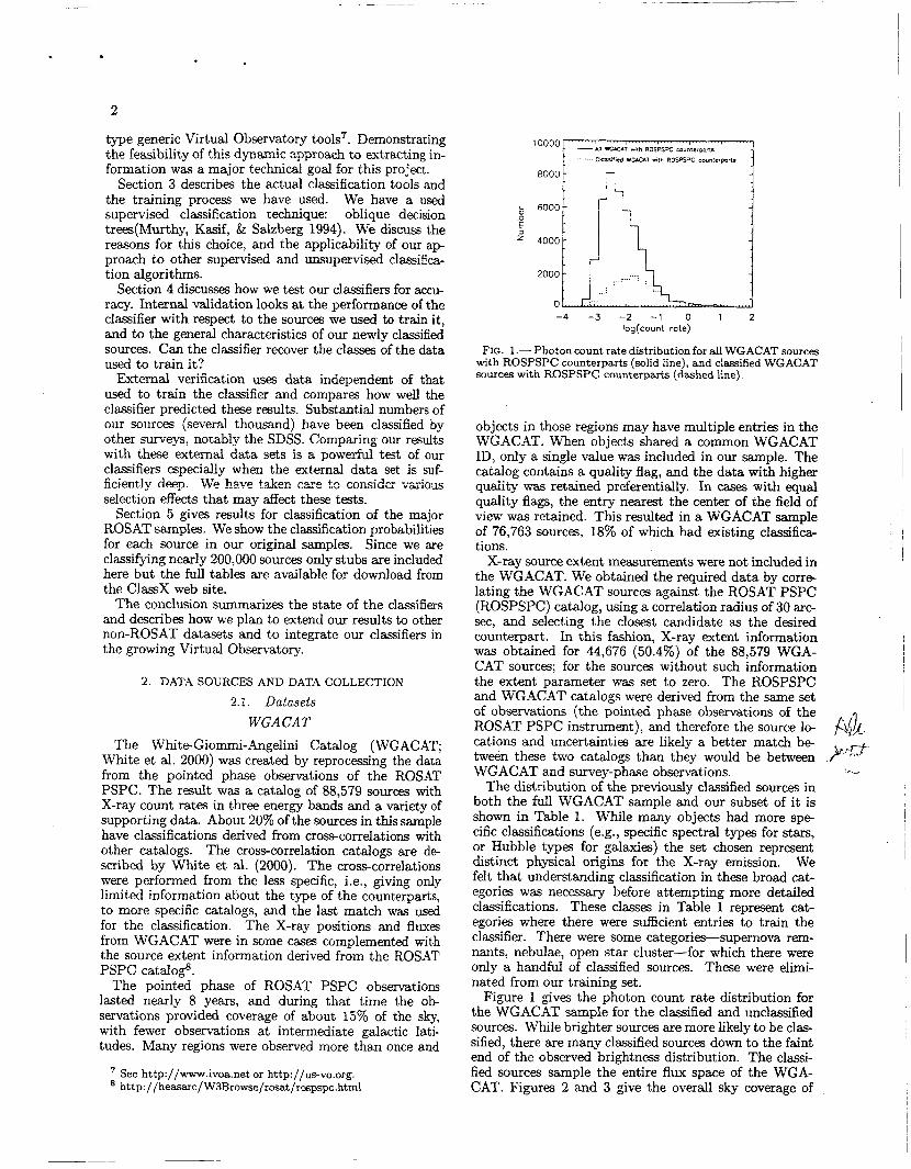
FIG. 1.- Photon count rate distribution for all WGACAT sources with ROSPSPC counterparts (solid line), and classified WGACAT sources with ROSPSPC counterparts (dashed line).

objects in those regions may have multiple entries in the WGACAT. When objects shared a common WGACAT ID, only a single value was included in our sample. The catalog contains a quality flag, and the data with higher quaiity was retained preferentially. In cases with equal quality flags, the entry nearest the center of the field of view was retained. This resulted in a WGACAT sample of 76,763 sources, 18% of which had existing classifications.

X-ray source extent measurements were not included in the WGACAT. We obtained the required data by corre- lating the WGACAT sources against the ROSAT PSPC (ROSPSPC) catalog, using a correlation radius of 30 arcsec, and selecting the closest candidate as the desired counterpart. In this fashion, X-ray extent information was obtained for 44,676 (50.4%) of the 88,579 WGA- CAT sources; for the sources without such information the extent parameter was set to zero. The ROSPSPC and WGACAT catalogs were derived from the same set of observations (the pointed phase observations of the ROSAT PSPC instrument), and therefore the source lo- cations and uncertainties are likely a better match between these two catalogs than they would be between > r p p WGACAT and survey-phase observations. r 4

The distribution of the previously classified sources in both the full WGACAT sample and our subset of it is shown in Table 1. While rnky objects had more s p e cific classifications (e.g., specific spectral types for stars, or Hubble types for galaxies) the set chosen represent distinct physical origins for the X-ray emission. We felt that understanding classification in these broad categories was necessary before attempting more detailed classifications. These classes in Table 1 represent categories where there were sufficient entries to train the classifier. There were some categories-supernova rem- nants, nebulae, open star cluster-for which there were only a handful of classified sources. These were eliminated from our training set.

Fi,gre 1 gives the photon count rate distribution for the WGACAT sample for the classified and unclassified sources. While brighter sources are more likely to be classified, there are many classified sources down to the faint end of the observed brightness distribution. The classified sources sample the entire flux space of the WGA- CAT. Figures 2 and 3 give the overall sky coverage of

FIG. 2.- Galactic distribution of all WGACAT sources.

FIG. 3.- Galactic distribution of classified WGACAT sources.

W S B S C 5 x 1 0 4 r """ '

0 -4 -3 -2 - 1 0 1 2

log(count rote:

FIG. 4.- Photon count rate distribution for RASS BSC (solid line) and RASS FSC (dashed line) sources.

the WGACAT sources for both the entire sample and the classified sources. Although the WGACAT source distribution is highly non-uniform, there is no major difference between the distributions of the (known) classified WGACAT objects and the entire catalog.

ROSAT All Sky Survey The ROSAT All-Sky Survey (RASS) catalogs (Voges et

al. 1999) contain X-ray sources detected during the survey phase of the ROSAT mission with the PSPC instrument. The entire sky was surveyed with exposures highest towards the ecliptic poles. While the survey covers

-4 - 3 -2 - 1 0 1 2 iog(count rote)

FIG. 5.- Photon count rate distribution for all FUSS (solid line) and classified RASS (dashed line) sources.

FIG. 6. - Galactic distribution of all RASS sources.

FIG. 7.--- Galactic distribution of classified RASS sources.

the entire sky, it is generally less deep than pointed observations. Overall 124,735 objects were detected: 18,811 of these were published in the RASS Bright Source Catalog (BSC) and 105,924 in the Faint Source Catalog (FSC).

Figures 4 and 5 give the photon count rate distribution of the RASS classified and unclassified sources. Since the classified sources were restricted to the BSC, the sam- pling of faint objects is quite poor. On the other hand the sky distribution of objects is much more uniform, which is seen in Figures 6 and 7. While there is a marked increase towards the ecliptic poles, the enormous contrasts

4

seen in the sky distribution of the WGACAT sources are not present in this sample.

2.2. The ClassX Pipeline The ClassX processing pipeline gathers the data used

for classification. A generic pipeline that can gather data from many catalogs in many wavebands was constructed for ClassX and we have looked at many different sources of information. However in this paper only X-ray, o p tical, and radio data were used. The catalogs used and information extracted are shown in Table 2. The correla- tive data from each band is gathered separately, filtered, and then combined to form a single package of data for use by the classifier itself. The classifiers X, and XOR described further in Section 3.5. The ClassX pipeline makes extensive use of the standard representation of tabular and catalog data developed in the Virtual Ob- servatory initiative, VOTable (Ochsenbein et al. 2000).

Optical counterparts of X-ray sources are found using a search radius of 30 arcsec; this gives a reasonable completeness level while keeping the number of chance coin- cidences manageable. The correlations were done using the VizieR (Ochsenbein, Bauer, & Marcout 2000) system.

If no counterpart was found, the object was dropped from consideration for use by classifiers needing information from that waveband. If a single counterpart was found, then the data from that counterpart was used. When multiple counterparts were found, a rule for resolv- ing the ambi,@y was needed. Both nearest and brightest counterparts were tried. Using the brightest counterpart was found to provide generally more accurate r e sults, however, a function combining the two would likely be better still. We have generally used the brightest candidate counterpart.

For radio data, only the existence or non-existence of the radio counterpart was used in the classifier. The combination of the NVSS and SUMSS catalogs gave us radio coverage over approximately 92% of the sky. Since the determination of the coverage boundaries for the S U M S surveys is non-trivial, data in the 8% region not covered was treated as having no counterpart. Even in classes where radio counterparts are most frequently found, most objects do not have a radio counterpart. So the 8% of the sky remaining does not seem to cause a significant bias.

In the final step before use by the classifier, the data from all tables were combined to produce a pair of files for input to the classifier. Only data for which all parameters required by the classifier were available (either from the table or by use of a default value) were included in the final sample.

2.3. Counterpart Validity The errors in the X-ray positions of the objects in the

WGACAT and RASS samples are relatively large com- pared to the typical separation of objects detected in the USNO-B survey. When we search for optical counterparts to the X-ray sources, we look for the brightest object within 30 arcsec of the nominal X-ray position. Almost all objects have at least one candidate counterpart within 30 arcsec and on average about 5 objects axe seen within the limiting radius. How much confidence can we have in the validity of our cross-identification

with optical and radio sources? Since we do not perform follow-up observations, this question can only be addressed statistically.

One powerful check on the validity of the identifications is to look for counterparts at positions near but slightly oifset from the nominal positions. Both the WGACAT and, to a lesser extent, RASS sources have non-uniform coverage, so that inferences drawn using the statistics of objects over the entire sky are not necessarily appropriate. So in addition to the actual correlation of each object in the WGACAT and RASS samples with the USNO-B survey, we also correlated a point 6 arcmin away at a random position angle. If our cross-correlations were dominated by spurious cross-identifications-i.e., the o p tical counterparts had no relation to the x-ray sources- then we would expect that the statistics of cross-match between the nominal target positions and the offset positions would be similar. By searching for a set of virtual control objects relatively near the actual objects- much closer than the 2 degree field of view of the ROSAT PSPC-our control sample is subject to the same sample biases as the real data.

It is certainly possible that some X-ray sources may have an extent comparabie to our 6 arcmin o&t, e.g., clusters of galaxies or nearby galaxies. However tGs will tend to lessen differences between the nominal and offset samples so that any observed difference between the samples should be considered a lower limit.

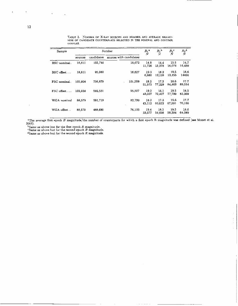
Table 3 shows that there are very significant variations between the actual objects and the control sample. The effect is overwhelming in the RASS BSC sample. There the brightnesses of the candidate optical counterparts are about 4 ma-pitudes greater than for the control sample. A 4 magnitude brightness offset corresponds to a factor of about 200 in the surface density of sources. Clearly the counterparts picked out for the RASS BSC are very special objects so that it seems unlikely that there can be more than a few percent of the counterparts chosen can be unrelated to the X-ray source.

We should note that finding an optical object associated with the X-ray source is distinct from finding the optical counterpart to the X-ray source. For example, consider an X-ray detected cluster of galaxies. Here our procedure might select a particular galaxy in that cluster as our candidate counterpart. While this galaxy is associated with the X-ray source, it would not be correct to identify the actual source of the observed X-ray emission as a galaxy.g

The RASS FSC and WGACAT samples are much deeper so that we would anticipate that counterparts would be fainter. This is borne out in Table 3 but the selected candidate counterparts to the nominal sample are still approximately a magitude brighter than for the offset control sample. This suggests that while there is some contamination of these samples, most of our candidate counterparts are still associated with the X-ray source. If our optical sources are uniformly distributed in space so that we have a ZI-'.~ brightness distribution, a one magnitude shift in magnitudes corresponds to a

Since our classifier uses purely empirical techniques, the classifier might still handle such clusters correctly. Even though the cross-identification is 'wrong', if this happened consistently the classifier will be trained to correctly recognize these objects as clusters.

5

factor of 4 of the surface density of objects. We might expect that 20% of our selected counterparts are not associated with the X-ray source. In many of these cases, the actual X-ray counterpart may have been one of the candidate counterparts but not the brightest within the 30 arcsec radius.

The number of counterparts near the nominal positions is substantially greater than near the offset position. Given than only a tiny fraction of optical objects have X-ray emission detected by ROSAT, we would expect that the number of optical counterparts near the nominal positions would be increased by the number of optical sources associated with the X-ray source, Le., we get the random background plus the signal. For some X-ray sources there may be multiple optical objects as sociated with it. For the fainter samples the total number of candidates is roughly consistent with there being one associated optical source for each X-ray object. For the BSC sample, the excess of sources near the nominal posi- . tions is substantially greater than the number of objects in the sample so that on average more than 3 optical sources are associated with the X-ray sources. These likely include many clusters of galaxies where a number cf gdaxies xc f ~ z d i i e ~ the cefiter of the X-ray emissions.

While we cannot, and do not, assert the validity of any specific positional association, the analysis of the statistical properties of the counterparts assures us that overall, they are dominated by real associations.

3. CLASSIFICATION TECHNIQUES 3.1. Introduction

Classification is the process of mapping the observable characteristics of an object to a set of classes that typically represent different physical types; a classifier is the implementation of a classification algorithm to perform this mapping. We consider here methods for supervised classificntion, meaning that a human expert both has determined into what classes an object may be categorized and also has provided a set of sample objects wit.h known classes. This set of known objects, called the.training set, is used by the classification programs to learn how to classify objects. The process of creating such a classifier for a particular data set is usually called training.

There are also unsupervised classification algorithms (e.g., clustering, mixture models) that attempt to determine both the types of objects and how to separate them directly from the parmeter-space distribution of the unclassified sample. We have chosen to work primarily with supervised classification methods, however, since we understand much of the underlying physics for the electro- magnetic emissions that are measured, and we can thus choose intelligently from among the many measured parameters to build the best training sets and select the best classes.

There are two steps to construct a supervised classifier. In the training phase, the training set is used to decide how~the parameters ought to be weighted and combined in order to separate the various classes of objects. In the application phase, the weights determined in the trdning set are applied to a set of objects that do not have known classes in order to determine what their classes are likely to be.

If a problem has only a few important parameters,

then classification is usually an easy problem. For example, with two parameters one can often simply make a scatter-plot of the feature values and can determine graphically how to divide the plane into homogeneous regions where the objects are of the same classes. The classification problem becomes very hard, though, when there are many parameters to consider. Not only is the resulting ndimensional space difficult to visualize, but there are so many different combinations of parameters that techniques based on exhaustive searches of the parameter space become computationally infeasible. Prac- tical methods for classification then involve a heuristic approach intended to find a good-enough solution to the optimization problem.

3.2. Oblique Decision Trees There are several ‘dimensions’ that we can vary in

building classifiers. The input observational characteristics and the output physical classes can be varied. We can use different sets of training information, and we can vary the basic algorithm for classification. In this paper we report on results using only a single classifier algorithm, the OC1 system of oblique decision trees (Milrt.hy, Kasif, & Salzberg 1994) for a k e d set of output classes. We have chosen the OC1 algorithm because it is freely available’0, its accuracy is comparable to the best available algorithms, and it is sufficiently fast (in both training and application). An additional benefit is that the decision tree can be examined after it has been trained to determine the key criteria for classification; this is difficult with, for example, neural networks.

Conceptually the oblique decision tree classifier is rather straightforward. It considers the n-space defined by the set of n input observational characteristics, where each characteristic is treated as a continuous variable. A binary tree is constructed in which at each node a plane in the n-space (described by a linear combination of the parameters) divides the objects into two groups. The first node represents a plane that divides the space into two regions. Objects are sifted down the left or right branches of the tree depending on which side of the plane they fall. The next node represents another plane that further divides the two sub-spaces. Ultimately one reaches a leaf node of the tree where all the objects in the region are assigned to a single class. Some parts of parameter space may be well delineated by only a few planes, while other parts might require many planes in order to separate complex distributions.

Oblique decision trees are difficult to construct because there are many possible planes to consider at each tree node. OC1 includes a flexible and efficient algorithm for creating a decision tree given a training set. See the Murthy et al. (1994) paper for full details; we describe here some key features of the algorithm.

OC1 uses a “greedy” algorithm in the initial tree construction. It first attempts to find the plane in the n- space that most cleanly divides the training set sample into two samples having distinct sets of classes. Vari- ous impurity measures are available for determining the quality of a particular split. It then repeats the process recursively for the sub-space on the two sides of the divid- ing plane. The algorithm continues until each remaining

lo http://www.tigr.org/-salzberg/announce-ocLhtm1

. 6

subregion is perfectly classified, with all included training set objects having the same class.

In most cases this initial tree divides the parameter space too finely. For example, some leaf nodes may contain only a single object, picked out by planes that separate it from a mass of nearby objects having different classes but with similar parameters. The tree overfits the training set data, tracking details much more closely than is justified. To address this OC1 prunes its decision tree. A fraction of the training set objects is reserved during the initial tree construction. This pruning sample is used to test the decision tree; decision nodes are eliminated if their removal does not reduce the classification accuracy for the pruning sample. The final tree does not classify the training set perfectly (some subregions contain multiple classes of objects), but it has higher overall accuracy than the original overfitted tree.

Oblique decision tree classifiers are not the only pos sible choices: other commonly used algorithms include neural networks, nearest-neighbor methods, and axis- parallel decision trees. See White (1997, 2000) for discussion of some astronomical applications and a more detailed comparison of these algorithms.

3.3. Voting Decision Trees and Classification Probabilities

We have improved on the accuracy of the classification by using not just a single tree, but rather a group of 10 trees that vote (White et al. 2000). This multiple- tree approach has been shown to be effective at improv- ing the accuracy of classifiers (Heath, Kasif, &: Salzberg 1996). OC1 uses a complex search algorithm that includes some randomization to avoid the classic problem of getting stuck in local minima in the many-dimensional search space. Thus, one can run OC1 many times using different seeds for the random number generator to produce many different trees.

Heath et al. (1996) used a simple majority voting scheme: classify the object with each tree and then count the number of votes for each class. We have improved on this by using a weighted voting scheme, where each tree splits its vote between classes depending on the pop- ulations of the classes &om the training set at that leaf. (Recall that after pruning a leaf may contain objects of several different classes.) If an object winds up at a leaf node with N training set objects of which L, are of class a (i = l...C), the tree’s fractional vote in favor of classification i is (Li + l ) / (N+C). (The particular form used for the ratio was derived from the binomial statistics at the leaf.) The votes from all 10 trees are averaged to produce a vector of probabilities that an object belongs to each of the possible classes in the training sample. We associate the largest element of this vector with the ‘class’ of the source.

3.4. The Output Classes There are many distinct classes of X-ray sources, and

one of the goals of this research is to understand the level of detail to which we can successfully distinguish such sources with the information we have at hand. In practice in this initial effort we have tended to be con- servative, using only six basic classes (Table 1).

A problem that needs to be addressed in the classifier design is that the same astronomical object may legiti-

mately belong to very different object types, especially as viewed from different wavelengths. While the X-ray properties of an X-ray binary are likely to be dominated by the accretion onto the compact companion, the optical appearance of the system may be that of, say, a normal Rstar-and it may be categorized as such in some catalogs. Similarly, while the X-ray emission of a cluster of galaxies originates mostly in the intracluster gas, the cluster optical or infrared counterpart would typically be a cluster galaxy.

These ambiguities complicate all phases of the classification, including construction of training sets, the training process itself, and interpreting the results. All classification errors are not equally bad when the classes are ambiguous. Clearly if the classifier confuses QSOs with AGNs, this is not nearly as serious as confusing AGNs with stars. We will return to these issues below in our discussion of the results.

3.5. ClassX Classifiers We introduce here four ‘basic’ ClassX classifiers de-

rived from the WGACAT and RASS BSC data (Table 2).

how the amount and the nature of the information fed into a classifier affects classification results. The FUSS- X and WGACAT-X classifiers use ROSAT data only, including positional information. The RASSXOR and WGACAT-XOR classifiers additionally use optical data for the optical counterparts and a flag indicating whether the source has or does not have a radio counterpart in the NVSS and SUMSS surveys; objects for which no optical counterpart could be found were not used in the training of these classifiers. All four illustrative classifiers are trained to distin,&h the same ‘basic’ set of classes: stars, white dwarfs (WD), X-ray binaries (XRB), AGNs, galaxies, and clusters of galaxies.

Many more classifiers, typically involving larger sets of classes and class attributes, are available at the ClassX web site. We describe one of them, in addition to the four mentioned above, WGACAT-XeOR. This ‘ex- tended’ classifier operates with a larger set of X-ray parameters and contains more detailed spectral information about X-ray sources. Specifically, it uses count rates in three energy bands as selected in the WGACAT and four WGACAT ‘hardness’ parameters, given by the count rate ratios in four different energy bands. This classifier also covers a wider set of classes, including three spectral groups of stars (0-F5, F6-G, K-M) and separate classes of AGNs and QSOs. Other classes are WD, XRB, and galaxy, however, unlike the basic class set, the cluster of galaxies class is not included.

They 1~5ed in s~ .&s~A&, & s ? s ~ G ~ t o illi&,i&,e

4. VERIFICATION

4.1. Cross- Validation and Classifier Characterization The statistical nature of ClassX classifiers means that

one has to have some measure of the quality of a classifier to tell if the classification results are of any value. To adequately assess a classifier and interpret classification results one would also need to know what are the differences between the classes and how relevant these differences are in a particular application of the classification results. In the following, we describe some methods to assess the quality of ClassX classifiers, and intro-

7

1 0 WGACAT-X ClaSsX class 1 - S T A R - g 7 5 - %CAT-xo N=5203 - $ 50-

2 2 5 - N=4310 -

.- 5 7 5 - N=16 - 2 25 - -

1 0 3 - XRB 5 7 5 - N=84 - N=100 - S O -

2 .25- -

.- 5 . 75 - N=4278 - 2; 50- N=3471 - 2 25- -

5 7 5 - N=364 - 2 50- N=491 - 2 2 5 - -

c - 1 0 - 2-WD

$ 50- N = 5 - c I

4

b. I - -

1 0 . 4 - AGN

c I 1 I

1 0 5 - GALAXY

c I I

6 - CLUSTER .- 5 75-N=802 - 0 50- N = R 7 0 2 2 5 -

4

c I I I ’

duce a quantitative characterization of both the classifiers (e.g.: reliability and completeness of classification, classifier preference) and classes (e.g. , class affinity).

A natural dataset to use to confirm the quality of a classifier is the training set that was used to develop it. The classifiers are tested using Sfold cross-validtition. The training set is divided into 5 equal-sized, randomly selected subsets (“folds”). Setting aside the first fold, 10 decision trees are constructed by training on the other 4 folds. Then the trees are tested for accuracy on the first fold, which was not used in the training. This process is repeated 5 times, each time holding back a different fold. When this is complete, we have classified the entire training sample. This standard technique avoids the overly optimistic results for classification accuracy one would get if one simply trained the classifier on all the data and then tested it on the same data’’.

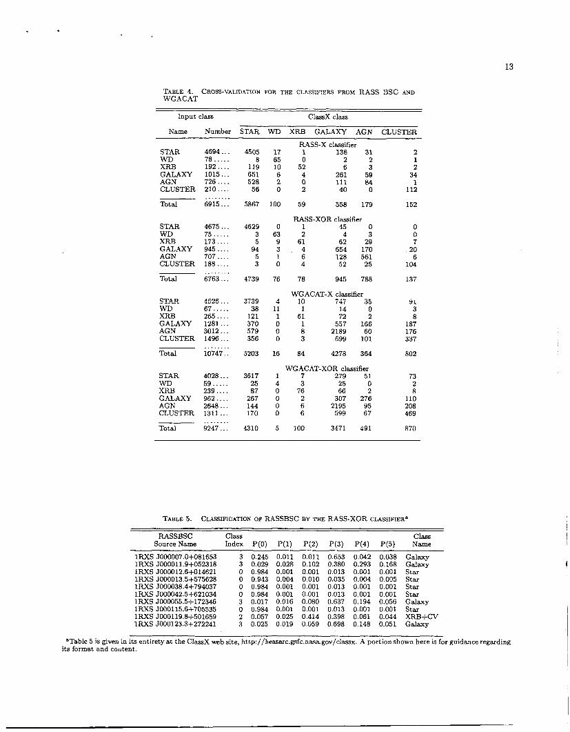
The results of cross-validation can be viewed as a matrix with the input classes as the column headers and the row headers as the output classes (see Table 4). For a perfect classifier, only the diagonal of the matrix would be populated. In practice the ratio of diagonal to off- diagonal elements gives us an immediate sense of how well the classifier has worked. In most cases the accuracy of the classifier is going to be higher for the training set sample than for originally unclassified sources, because the population of unclassified sources may differ system- atically from known sources (e.g., by being fainter.) On the other hand, some disagreements between the OC1 classifier and the training set classification are the r e sult of classification errors in the (imperfect) training set. There the cross-validation results correspondingly underestimate the classifier accuracy.

The cross-validation results are shown in Figures 8-9. Each panel in these figures gives the fraction of objects in input class categories, classified by ClassX as objects of a given type. The diagonal across the panels gives, therefore, the fraction of correctly classified sources in each class and thus represents reliability of classification. Because of closeness, or afinity, of some classes in the parameter phase space (e-g., galaxies and AGNs), the classifier may place some objects of a given input class into a class with similar properties. Figures 8-9 characterize quantitatively such class d n i t y . One can infer, for instance, from Figure 8 that there is a substantial affinity between the ROSAT BSC galaxies and AGNs when only X-ray properties are considered. Addition of optical information decreases that affinity quite noticeably. At the same time clusters of galaxies are obviously dis tinctly different from AGNs in the X-ray. The affinity relationships between the classes are somewhat different for objects from WGACAT (Figure 9).

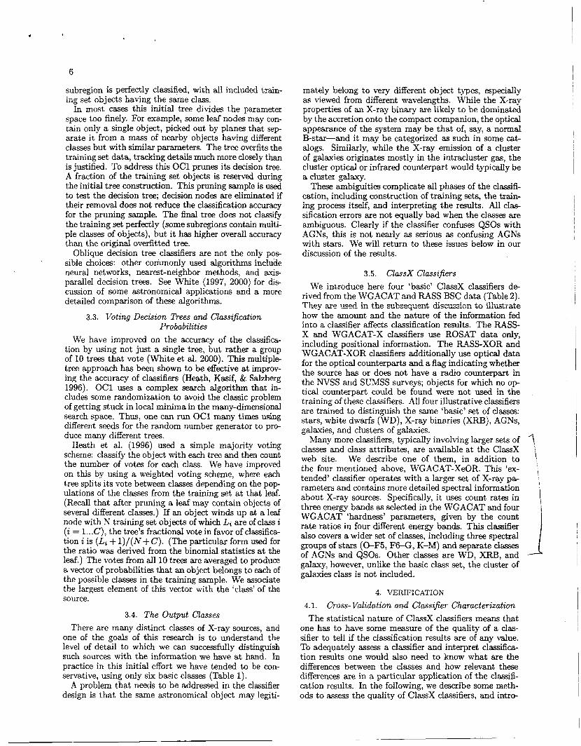
In Figures 10 and 11, each panel gives the fraction of input objects of a given type classified by ClassX into different class categories. The diagonal across the panels shows US how complete is the placement of sample objects of a given type into thc correct class category, giving us a measure of classification completeness. In general Figures 10 and 11 show US the classifier preferences as it

Note that classifiers trained with 80% of the data are only used in cross-validation. The classifiers installed at the ClassX web site and used in this paper for classifications of unknown objects are trained using the entire sample of pre-classified sources.

FIG. 8.- Classifier crossvalidation: Distribution of input classes within a given ClassX class (class affinity). Light and dark shadings refer to the results for the classifiers using X-ray data only (from ROSAT) and X-ray plus optical and radio data, respectively. Each panel shows the fraction of each of the input classes assigned by ClassX the class name given in the panel. Ideally that fraction must be 100% for the input class having the same name, which means 100% reliable classification for that name. In reality, ClassX assigns the given name also to a fraction of objects whose actual class has a d3eraul IILLIII~, which happens more often for classes whose affinity with the given class in the parameter phase space is the largest.

Input class1 2 3 4 5 6 $ 7 4 ~ *L) *&& 4G& G4%%sT.@

FIG. 9.- Same as in Figure 8 but for the classifiers derived from WG AC AT.

8

E 25- I

1 0 5 75- < 50-

1.0 2 25-

g 75-

- 5 50-

-I 50 N=100 E 25 - * I

- I I I 4 - AGN N=3012 - N=2646 - -

5 - GALAXY -

N= 1281 - N=962 -

FIG. 10.- Classifier cross-validation: Distribution of ClassX classes within a given input class (classifier preference). Each panel exhibits the fraction of objects of the given input class in each ClassX class. .4n ideal classifier would assign to all objects in a given input class the name of that class. In reality, the classifier assigns different names, showing different preference for different names. In the case of a good classifier, the preference is highest for the name of the given input class.

.- ?; .50 E .25

1 .o

3 o .50

*

g .75

N=4626 N=4020

VGACAT-XO -

I N=67 N=59

3 - XRB N=265 N=23D

ClassXc lass l 2 3 4 5 6 'D 'e& 4Q Gwc&~.e

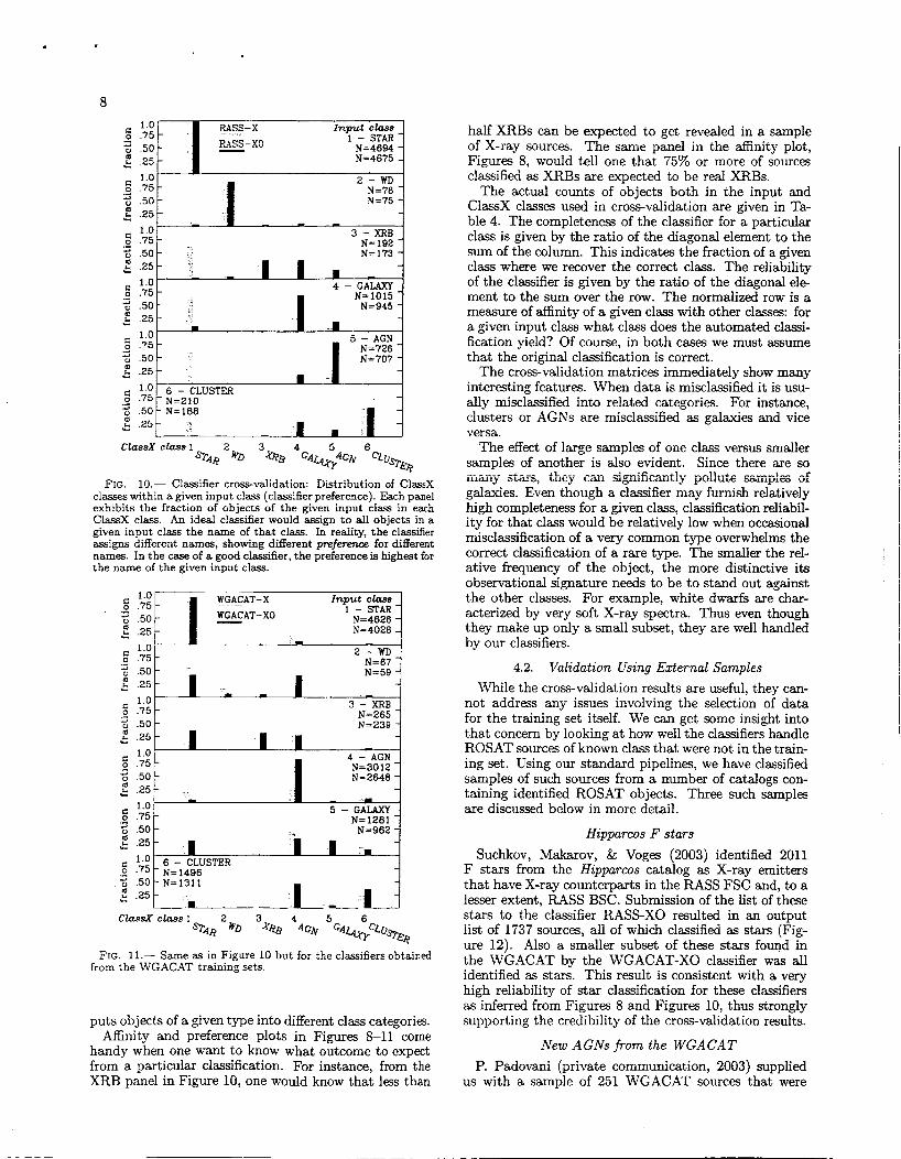
FIG. 11.- Same as in Figure 10 but for the classifiers obtained from the WGACAT training sets.

puts objects of a given type into different class categories. Affinity and preference plots in Figures 8-11 come

handy when one want to know what outcome to expect from a particular classification. For instance, from the XRB panel in Figure 10, one would know that less than

half XRBs can be expected to get revealed in a sample of X-ray sources. The same panel in the affinity plot, Figures 8, would tell one that 75% or more of sources classified as XRBs are expected to be real XRBs.

The actual counts of objects both in the input and CiassX classes used in cross-validation are given in Ta- ble 4. The completeness of the classifier for a particular class is given by the ratio of the diagonal element to the sum of the column. This indicates the fraction of a given class where we recover the correct class. The reliability of the classifier is given by the ratio of the diagonal element to the sum over the row. The normalized row is a measure of affinity of a given class with other classes: for a given input class what class does the automated classification yield? Of course, in both cases we must assume that the original classification is correct.

The cross-validation matrices immediately show many interesting features. When data is misclassified it is usually misclassified into related categories. For instance, clusters or AGNs are misclassified as galaxies and vice versa.

The effect of large samples of one class versus smaller samples of another is also evident. Since there are so l?i&-lj- st&-s, tklej. galaxies. Even though a classifier may furnish relatively high completeness for a given class, classification reliability for that class would be relatively low when occasional misclassification of a very common type overwhelms the correct classification of a rare type. The smaller the rel- ative frequency of the object, the more distinctive its observational signature needs to be to stand out against. the other classes. For example, white dwarfs are characterized by very soft X-ray spectra. Thus even though they make up only a small subset, they are well handled by our classifiers.

4.2. Validation Using External Samples While the cross-validation results are useful, they can-

not address any issues involving the selection of data for the training set itself. We can get some insight into that concern by looking at how well the classifiers handle ROSAT sources of known class that were not in the training set. Using our standard pipelines, we have classified samples of such sources from a number of catalogs containing identified ROSAT objects. Three such samples are discussed below in more detail.

&oq~~c.&ly po&Gte --+.& of

Hipparcos F stars Suchkov, Makarov, & Voges (2003) identified 2011

F stars from the Hzpparws catalog as X-ray emitters that have X-ray counterparts in the FUSS FSC and, to a lesser extent, RASS BSC. Submission of the list of these stars to the classifier RASSXO resulted in an output list of 1737 sources, all of which classified as stars (Fig- ure 12). Also a smaller subset of these stars found in the WGACAT by the WGACAT-XO classifier was all identified as stars. This result is consistent with a very high reliability of star classification for these classifiers as inferred from Figures 8 and Fi,ves 10, thus strongly supporting the credibility of the cross-validation results.

New AGNs from the WGACAT P. Padovani (private communication, 2003) supplied

us with a sample of 251 WGACAT sources that were

9 1.0

.75

z .50 m - .25 0

. - '." I New WGACAT AGNs I I N=42

N=204

Sloan AGNs

5 .50 .25

FIG. 12.- Class distribution for a sample of X-ray F stars (upper

samples were classified by the classifiers RASSXO (light shading) and WGACAT-XO (dark shading). Classification shown in light gray in the lower panel is discussed in text. The sample of F stars is from the paper by Suchkov et al. (2003), The sample in the middle panel is due to P. Padovani. It comprises mostly the sources from Landt et al. (2001) and Perlman et al. (1998), which were drawn from the previously unclassified WGACAT sources and identified as AGNs. The sample in the lower panel comprises AGNs from the Sloan Digital Sky Survey that were found to have X-ray counterparts in the ROSAT All Sky Survey catalogs (Anderson et al. 2003).

---- 1\ ---I &-.- r..-..lrr -C A P h L /-:AAIA -..A l,....,.- ,..,-,,l-\ T h - p c u A e L / c&I,U Y I " " " U A A ' y ' G " "A '."I." , . A L A U U . b -1.. 1 " V " L . l y'uYL.'"/. Illr

identified by him and his collaborators as various types of quasars and AGNs (Landt et al. 2001; Perlman et al. 1998; Padovani et al. in preparation). The results of classification of this sample with the WGACAT-XO and RASS-XO classifiers are shown in the middle panel of Figure 12. The classifier does a good job in distinguishing the AGNs from all other classes.

AGNs from the Sloan Digital Sky Survey The Sloan Digital Sky Survey (SDSS) is a deep photo-

metric and spectroscopic optical survey, where a large number of sources were spectroscopically identified as AGNs. For more than 1200 Sloan AGNs, Anderson et al. (2003) found X-ray counterparts in the ROSAT All Sky Survey. We used a sample of 964 of these AGNs to test the performance of the ClassX classifiers. The results of the classification of that sample are shown in the lower panel of Figxe 12. The c1assiSer performance is very good in terms of differentiating the Sloan AGNs from galactic X-ray sources (stars, white dwarfs, XRBs) and clusters of galaxies. The WGACAT-XO classifier eas ily differentiates these AGNs from galaxies; the FUSS- XO classifier is less successful in such a differentiation, possibly because it is trained with substantially brighter objects.

4.3. Classification Accuracy as a Function of Brightness.

CrJ -'I STAR i

- 1.01 -

2 3 4 5 6 -2.5 log (count rate)

FIG. 13.- Fraction of the WGACAT training set sources cor-

tion of X-ray brightness (defined as -2.5log(count rate)). The actual number of sources of a given class in each brightness bin is also shown.

rect!:~ ci~sif ied $7 the c!zssifier WC,.AC.A_T-XQ, disp!ayyed = % f-21~-

One clear distinction between the classified and unclassified sources is that the classified sources are generally brighter. One may expect. t,hat classification accuracy for fainter sources would be different. As one can see in Figure 13, classification accuracy does indeed vary with X-ray brightness. Interestingly enough, the degree and even the sense of that variation is not the same for different classes. In the case of AGNs, the accuracy drops from 80% at the bright end to below 70% at the faint end of the distribution. In contrast the classification accuracy of clusters of galaxies tends to increase rather than decrease toward faint sources. For stars, accuracy variation is rather small, with a slight tendency to accuracy degradation at the faint end. The accuracy variation is obviously important to know for interpretation of classification results, especially when a classifier is used in a parameter domain substantially different from that of the training data.

4.4. Limits and Issues While our validation of the classifiers is not entirely se-

cure, especially with regard to the cross-correlation errors and the effects of selection on the training set, several distinct lines of evidence suggest that these classifiers give reasonable classifications for their sources. While no single classifier is optimal for classifying all kinds of data, a classifier network that filters data through a series of classifiers can give reasonable results for a heterogeneous dataset. A scientist with more specialized requirements, such as completeness without regard to purity for galaxies, or perhaps a pure sample of early type stars, may wish to choose a classifier that optimizes that property.

The classifiers have been built from heterogeneous data sources, which are likely to have some fraction of incor- rect identifications. Pruned decision tree classifiers seem to be robust in the face of such contamination, so that

10

one can even use the classifiers to attempt to purify the input data set.

5 . SUMMARY OF RESULTS

Classification results from ClassX for the entire WGA- CAT and RASS datasets are available at the ClassX web site a t http://heasarc.gsfc.nasa.gov/classx. They are il- lustrated in Tables 5 and 6, which show the first few rows of two selected tables. In addition to these static classifications, more than

two dozen ClassX classifiers, readily accessible for the community for immediate use, are currently deployed at the ClassX web site. The web site contains a description of the input data format, which is the list of source coordinates, and the input/output options. All the classifiers are supplied with the information indicating the classifier class categories, parameters (attributes) to be used in classification and returned in the output, databases (catalogs) to be searched for the source information, and other relevant information. In the output, each classified source is supplied with classification probabilities for all classes, and is assigned a class name, which corresponds to the class with the highest classification probability.

for the source and used in classification. TL- -..&-..t -1”- nr\n+q:nr +hc. -oromnefi- ,..,l,.- -c.+.4c..rAA L,,G vul,puL, a w w b W I I Y L * ‘ L W ”llcl yc*Lcuub”w I-UW Ilr”I*b”L&&

6 . CONCLUSIONS

Classification of X-ray (or optical, infrared, etc.) sources into various categories of astronomical object types can rarely, if at all, be 100% accurate. The pres- ence of uncertainty inherent to classifications bawl an statistical methods immediately splits the very goal of classification into a set of different goals, which are often incompatible. As a result, any statement about classifier effectiveness would generally make sense only if the classification goal or task, with respect to which the effectiveness is considered, is indicated. For example, one may want either to isolate as complete as possible objects of a given class in a given sample, even at the expense of a larger fraction of misclassified sources, or to deal only with objects of a class identified with the highest possible degree of reliability, even at the expense of re- jecting many class objects that the classifier is unable to identify as such at the desired level of reliability. These different goals can be addressed in ClassX with different classifiers. One classifier can be effective in identifying to a high degree of completeness the members of a class, but classification reliability for identified class members may not be high enough. Still another classifier can be effective in delivering highly reliable class members but may miss many actual members of the same class.

Supervised classification techniques are a very powerful way of extending information about well-understood o b jects in a sample to the entire sample. For X-ray sources, it is possible to do classifications using just a few X-ray parameters as object attributes. Multiwavelength data can substantially improve the quality of the classifications, although adding data without regard to its quality or uniqueness does not necessarily help.

REFEl

Adelman, J. et al. 1999, BAAS 195,8204

Anderson, S. F. et al. 2003, AJ, 126, 2209

The ClassX classifications are useful for studying classes of objects, but the classification of any individual object should be taken as advisory rather than definitive. Human understanding and judgment is crucial in assess ment and interpretations of the results. This is especially true given the statistical nature of ClassX.

In ClassX, a substantial number of input (training) sources are required for each class t o effectively classify a sample. This number depends on the degree to which attributes of the class differ from those of other classes. In the case of white dwarfs, the FUSS-XO classifier trained with less than a hundred of these objects proved never- theless to be quite effective both in detecting the majority of actual white dwarfs in the (training) sample of many thousand objects and ensuring high reliability of white dwarf candidates.

We anticipate that modifications to the classifier algorithm that note when objects do not map well into existing classes will be needed to improve its detection capabilities for previously unknown object types (Laidler & White 2003). Currently the latter functionality can be emulated through appropriate analyses of classification probabilities provided by ClassX.

entire FUSS and WGA samples. However, for X-ray sources more than a factor of 10 fainter (e.g., Chan- dra and XMM sources), we anticipate substantial incom- pleteness in the large optical surveys. The Sloan Survey should do better here.

Optical information is critical to distin,@hing Galac- tic from extragalactic sources. Tt. i s less crucial for classifying clusters of galaxies and white dwarfs. The effect of infrared information in ClassX is generally similar to that from the optical in distinguishing broad classes. This information becomes increasingly useful in finer grained classification. A network of ClassX classifiers, each using a different set of object parameters (attributes) and even a different set of classes can provide a highly complete and reliable overall classification.

In general, the more detailed and accurate information is available to a classifier the more precise the classification results are.

The phase space of possible classifiers is very large. A substantial fraction of this effort was to learn a reasonable minimum of information to use.

Handling diverse sources of information is a major chal- lenge. Adoption of standard protocols and formats such as those now being developed in the Virtual Observatory is crucial in creating a fast and easy-to-use system.

..,.A-y*- Simnln m-ficc-irlnntifiritinn -..---l.**-”-vl y-.,.,-.---- nrnrdiiroc urnrk ,. well ..--- --- fnr the

We wish to thank L. Angelini, M. E. Donahue, S. A. Drake, P. Fernique, F. Genova, W. D. Pence, M. Post- man, M., and M. Wenger for numerous discussions of the project.

This work was funded through NASA’s Applied Infor- mation Systems Research Program under grant NAG5- 11019.

tENCES

Heath, D., Kasif, S., & Salzberg, S. 1996, in Cognitive Technology: In Search of a Humane Interface, eds. B. Gorayska & J. Mey (Amsterdam: Elsevier), p. 305

11

TABLE 1. ‘BASIC’ CLASSES AND THE XUtdBER OF CLASS OBJECTS IN THE WGA- CAT AND RASS BSC SAMPLES

- WGACAT RASS

Class all unique”

Star .................. 6027 4678 4694 WD (white dwarfs) ... 152 98 78 XRB (X-ray binaries)b 494 271 192 AGNC ................ 4589 3031 726 Galaxy ............... 1614 1305 1015 Cluster (of galaxies). . 1717 1508 210

Origin of X-ray emission

Corona or shocked stellar wind. Hot atmosphere. Accretion disk of a neutron star or black hole. Central accretion disk, XRBs, galactic wind XRBs, hot corona, galactic wind. Hot intracluster gas.

- Unclassified.. ......... 73986 65872 Total ................. 88579 76763 6915

“In the case of multipe entries for a source, only the entry closest to the center of the PSPC field is included. bIncluding cataclysmic variables. =Including quasars, radio galaxies, and BL Lac galaxies.

TABLE 2. CLASS ATTRIBUTES (OBJECT PARAMETERS) USED BY THE FOUR ’BA- SIC’ CLASSX CLASSIFIERS

Classifier”

xo x Galactic longitude, I ~ I . . .. Input Y Y Galactic latitude, b I I ..... Input Y Y X-ray brightnessb.. ........ X-ray data Hardness ratio 1, HRlc. . . X-ray data Y Y Hardness ratio 2, HR2‘. .. X-ray data Y Y X-ray extent (source size)d X-ray data Y Y Blue magnitude, Be ...... Optical data Y n Red magnitude, R e . . ..... Optical data Y n Radio counterpart flag‘. .. Radio data Y n

Attribute name Attribute Source

Y Y

“X for WGACAT-X and RASS-X classifiers, XO for WGACAT-XO and R4SS-XO classifiers. Parameter required by a classifier is indicated

bDefined as -2.5 log(count rate). CFrom RASS or computed from WGACAT. dFrom RASS or ROSPSPC (for WGACAT) if available, else 0. eFrom the USNO B1 catalog. ‘1 if counterpart found in XTSS or SUMSS, else 0.

by ‘y’, otherwise ‘n’.

Helfand, D. J., Schnee, S., Becker, R. H., White, R. L., & McMahon, R. G. 1999, ApJ, 117,1568

Laidler, V. G., & White, R. L. 2003, in Statistical Challenges in Astronomy 111, eds. E. D. Feigelson & G. J. Babu (New York: Springer), p. 453

Landt, H., Padovani, P., Perlman, E., Giommi, P., Bignall, H., & Tsiomis, A. 2001, MNRAS, 323,757

Monet, D. G., et al. 2003 AJ, 125,984 Murthy, S. K., Kasif, S., & Salzberg, S. 1994, J. Artif. Intell. Res., 2, 1

Ochsenbein, F., Albrecht, M., Brighton, A., Fernique, P., Guillaume, D., Hanisch, R., & Wicenec, A. 2000, in Astronomical Data Analysis Software and Systems IX, Astron. SOC. Pacific Conference Series, N. Manset, C. Veillet, and D. Crabtree, eds., 216, 83. Also see http: //www.ivoa.net/twiki/bin/view/IVOA/IvoaVOTable for updates to the VOTable standard.

Ochsenbein, F., Bauer, P., & Marcout, J . 2000, A&AS 143, 230 Odewahn, S. C. 1995, PASP, 107, 770

Perlman, E. S., Padovani, P., Giommi, P., Sambruna, R., Jones,

Rutledge. R., Brunner. R. J., & Prince, T.A. 2000, ApJS 131, 335 L., Tsiomis, A., & Reynolds, J. 1998, AJ, 115, 1253

Salzberg,’S.,Chandar,’R., Ford, H., Murthy, S. K.,’&White, R. L. 1995, PASP, 107,279

Suchkov,A. A,, Makarov, V. V., & Voges, W. 2003, ApJ, 595,1206 Voges, W. et al. 1999, A&A, 349,389 Voges, W. et al. 2000, IAU Circ., 7432,l Weir, N. et al. 1995, PASP 107,1243 White, R. L. et al. 2000, ApJS, 126, 133 White, R. L. 1997, in Statistical Challenges in Modern Astronomy

11, eds. G. J . Babu & E. D. Feigelson (New York: Springer), p. 135

White, N. E., Giommi, P., Angelini, L. 2000, http://wgacat.gsfc.nasa.gov.

White, R. L. 2000, in ASP Conf. Ser., Vol. 216, Astronomical Data Analysis Software and Systems IX, eds. N. Manset, C. Veillet, & D. Crabtree (San Francisco: ASP), 577

Zhang, Y. & Zhao, Y. 2003, PASP 115, 1005

12

TABLE 3. ?;UMBER OF X-RAY SOURCES AND NUMBER AND AVERAGE BRIGHT- NESS OF CANDIDATE COUhTEWARTS SELECTED IN THE NOMINAL AND CONTROL S.4MPLES.

Sample Number Bia Rib Bz,' 2- d IV N rv

sources candidates sources with candidates

BSC nominal. 18,811 155,744 18,672 14.8 14.4 15.5 14.7 11,726 15,378 16,074 16,459

BSC offset . . . 18,811 95,980

FSC nominal. 105,924 736,879

FSC offset.. . . 105,924 592,531

WGA nominal 88,579 591,719

16,627 19.3 18.2 19.5 18.6 6,930 12,128 13,455 14401

101,559 18.2 17.3 18.6 17.7 51,573 77,229 84,463 89,014

95,507 19.2 18.1 19.5 18.5 43,027 70,427 77,799 83,369

82,799 18.2 17.3 18.6 17.7 43,112 60,622 67,581 70,186

WGA o&et . . 88,579 488,685 76,133 19.4 18.2 19.5 18.6 33,677 54,608 59,394 64,089

aThe average first epoch B magnitude/the number of counterparts for which a first epoch B magnitude was defined (see Monet et al.

-3ame as above but for the first epoch E magnitude. 'Same as above but for the second epoch B magnitude. dSame as above but for the second epoch R magnitude.

2003). L-

13

TABLE 4. WGACAT

CROSS-VALIDATION FC)R THE CL.4sS?F!EPS F?.OM RASS BSC .WD

Input class ClaSsX class _ - iyame Number STAR WD XRB GALAXY AGN CLUSTER

STAR 4694 .. . WD-- 78.. .. . XRB 192 . . . . GALAXY 1015.. . AGN 726 . . . . CLUSTER 210.. . .

Total 6915 .. . . . . . . . . .

STAR 4675 ... WD 75 ..... XRJ3 173.. . . GALAXY 945 . . . . AGN 707 . . . . CLUSTER 188.. . .

. . . . . . . . Total 6763 . . .

I STAR --_-I 4625.. . WD 67 ..... XRB 265 . . . . GALAXY 1281 . . . AGN 3012 .. . CLUSTER 1496 . . .

Total 10747.. . . . . . . . .

STAR 4028 .. . WD 59.. . . . XRJ3 239.. . . GALAXY 962.. . . AGN 2648 . . . CLUSTER 1311 .. .

Total 9247 . . . . . . . . . . .

4505 8

119 651 528 56

5867

4629 3 5

94 5 3

4739

070n “ I d . 7

38 121 370 579 356

5203

3617 25 87

267 144 170

4310

17 65 10 6 2 0

100

0 63 9 3 1 0

76

1 11 1 0 0 0

16

RASS-X classifier 1 138 31 0 2 2

52 6 3 4 261 59 0 111 64 2 40 0

59 558 179

FUSS-XOR classifier 1 45 0 2 4 3

61 62 29 4 654 170 6 128 561 4 52 25

78 945 788

WGACAT-X classifier - .- (41 35 .,.

I U

1 14 0 61 72 2 1 557 166 8 2189 60 3 699 101

84 4278 364

2 1 2

34 1

112

152

0 0 7

20 6

104

137

91 3 8

187 176 337

802

WGACAT-XOR classifier 1 7 279 51 73 4 3 25 0 2 0 76 66 2 8 0 2 307 276 110 0 6 2195 95 208 0 6 599 67 469

5 100 3471 491 870

TABLE 5. CLASSIFICATION OF RASSBSC BY THE RASS-XOR CLASSIFIER”

FUSSBSC Source Name

lRXS 5000007.0+081653 lRXS JOOOOl1.9+0523 18 lRXS 5000012.6+014621 lRXS 5000013.5+575628 lRXS 5000038.4+794037 lRXS 5000042.5+621034 lRXS JOOOO55.5.f 172346 lRXS 5000115.6+705535 lRXS 5000119.8+501659 lRXS J000123.3+272241

Class Index

3 3 0 0 0 0 3 0 2 3

P(0) 0.245 0.029 0.984 0.943 0.984

0.984 0.057 0.025

P(1) 0.011 0.028 0.001 0.004 0.001

0.984 0.001 0.017 0.016

0.001 0.025 0.019

P(2) 0.011 0.102 0.001 0.010 0.001 0.001 0.080 0.001 0.414 0.059

P(3) 0.653 0.380 0.013 0.035 0.013 0.013 0.637 0.013 0.398 0.698

P(4) 0.042 0.293 0.001 0.004 0.001 0.001 0.194 0.001 0.061 0.148

P(5) 0.038 0.168 0.001 0.005 0.001 0.001 0.056 0.001 0.044 0.051

~ ~

Class Name

Galaxy Galaxy s ta r Star s ta r s ta r Galaxy s ta r XRB+cv Galaxy

aTable 5 is given in its entirety at the ClassX web site, http://heasarc.gsfc.nasagov/classx. A portion shown here is for guidance regarding its format and content.

.

14

TABLE 6. CLASSIFICATION OF WGACAT BY THE WGACAT-XOH CLASSIFIER^

WGACAT Class Class Source Name Index P(0) P(1) P(2) P(3) P(4) P(5) Name

~~

lWGA 51052.2+5655 0 0.673 0.021 0.026 0.113 0.138 0.030 Star lWGA J1049.1+5656 0 0.673 0.021 0.026 0.113 0.138 0.030 Star lWGA 51055.2+5704 0 0.483 0.039 0.061 0.057 0.254 0.106 Star lWGA J1049.8+5705 0 0.483 0.039 0.061 0.057 0.254 0.106 Star lWGA 51052.4+5708 0 0.483 0.039 0.061 0.057 0.254 0.106 Star lWGA 51053.8+5709 4 0.270 0.039 0.039 0.219 0.348 0.085 AGN lWGA J1052.0+5710 0 0.609 0.026 0.045 0.031 0.194 0.094 Star lWGA 51051.4+5711 0 0.483 0.039 0.061 0.057 0.254 0.106 Star lWGA 51053.3+5712 0 0.483 0.039 0.061 0.057 0.254 0.106 Star 1 WGA J1053.1+5714 0 0.483 0.039 0.061 0.057 0.254 0.106 Star

aTable 6 is given in its entirety at the ClassX web site, http://heasarc.gsfc.nasagov/cla.ssx. A portion shown here is for guidance regarding its format and content.

each as - nasa · felt that understanding classification in these broad cat- egories was necessary...

Documents