e81 final report

ENGR 081: Thermal Energy Conversion Biodiesel Production, Evaluation, and

Analysis

Steven Matos-Torres May 14, 2016

Matos-Torres 2

Table of Contents Abstract 3 Introduction 3

Procedures 5

Results 9

Discussion 12

Conclusion 14

Works Cited 15

Appendix A 16

Appendix B 19

Matos-Torres 3

Abstract:

This report analyzes how petro diesel fuel compares to two batches of biodiesel fuel. A

diesel test stand is used to collect various engine data for each type of fuel. The purpose of this

project is to recreate aspects of the E90 project Jonathan Martin ’12 did and determine if there

is a significant performance difference when using biodiesel fuel instead of petro diesel. The

main performance metrics used to compare the fuels were torque, engine speed, torque versus

speed, fuel flow, air flow, and fuel to air ratio. This report was able to provide a starting point

for comparison, but issues during experimentation resulted in the loss of the petro diesel fuel

level data, which threw off the comparisons for fuel flow and the fuel to air ratio.

Introduction:

Since the 1970s, the use of diesel fuel in the United States has increased steadily. In

2012 alone, there were 36,343,072,000 gallons of diesel fuel consumed just on highways.1 This

is an alarming, yet unsurprising statistic given that the United States uses more barrels of fuel

per day than any country in the world and more than the China, Japan, and India combined.2

The tremendous consumption of fossil fuels has prompted research and development of

alternative fuels to minimize the long-term effects of using fossil fuels. Biodiesel fuel made from

cooking oil may present itself as an adequate substitute. Biodiesel can be made from virgin or

waste cooking oil. Making this biodiesel fuel from waste cooking oil is important given that over

3 billion gallons of cooking oil are used per year in hotels and restaurants across the United

States.3

1 http://www.americanfuels.net/2014/04/us-on-highway-diesel-fuel-consumption.html 2 http://world.bymap.org/OilConsumption.html 3 https://www3.epa.gov/region9/waste/biodiesel/questions.html

Matos-Torres 4

This project was inspired by Jonathan Martin ’12, who produced biodiesel fuel from

various cooking oils and tested them on the diesel test stand in Hicks. Since there is only one

diesel test stand in Hicks and it would be a shame if biodiesel fuel from waste vegetable oil

ruined it, this project only tested biodiesel produced from virgin vegetable oil and compared

the data to petro diesel.

Two groups of E14 students were integral to this project. One group produced the

second batch of clean biodiesel and a batch of biodiesel from waste vegetable oil. The biodiesel

from waste oil was produced only to experiment with the filtration process and chemically

compare the product with clean biodiesel fuel. The other group was responsible for preparing

the test components of the project and creating a sample MATLAB Script for data acquisition.

This group rewired a multiplexer (figure 1) and made sure all of the transducers produced

voltages (figure 2).

Figure 1 (left): Multiplexer used for data acquisition Figure 2 (right): Transducers used to relay voltages to the multiplexer

During experimentation, the data for the different types of fuel was varied by manually

changing the speed of the engine from trial to trial with each individual fuel, but similar engine

speeds were used across trials for the different fuels. The engine behavior was also varied by

changing the electrical load the same way during each trial to see how the engine would

respond.

Matos-Torres 5

Procedures:

Producing Biodiesel Fuel:

Find an outlet and plug the stir plate into it. Count 20 pellets of NaOH and put them in a

2L Erlenmeyer flask with approximately 220-230 mL of methanol. Place a two-inch magnetic stir

bar in the Erlenmeyer flask. Put the Erlenmeyer flask on top of the stir plate. Set the stir plate to

“7” and stir until the NaOH completely dissolves. Once the NaOH completely dissolves, remove

the Erlenmeyer flask from the stir plate and add 1L of vegetable (soybean) oil. Cover the flask

with a rubber stopper and place the flask back on top of the stir plate. Let the contents of the

flask stir overnight.

The following day, turn off the stir plate and let the contents settle into two separate

layers. The top layer is the biodiesel fuel. Separate these layers by carefully pouring the layer of

biodiesel into a second 2L Erlenmeyer flask, making sure none of the other layer gets into the

second flask. Measure, in mL, how much biodiesel was separated into the second flask. Add

deionized water to the flask in a quantity that makes a 3:1 ratio of biodiesel to deionized water.

Add distilled vinegar to the flask in a quantity that makes a 2:1 ratio of deionized water to

vinegar. Put the rubber stopper on the flask and shake vigorously for 3 minutes. This completes

the first round of decanting. Repeat this separation and decanting process two more times,

only adding deionized water when decanting. After the third round of decanting, let the

contents settle and separate the layer of biodiesel. This is the final product.

Preparing the Diesel Test Stand:

Locate the power cables for the diesel test stand plug them into their outlets on the

wall. Turn on the computer and log onto the network. Insert the multiplexer into the top slot on

Matos-Torres 6

the back of the Agilent data acquisition device. Turn on the data acquisition device. Open

MATLAB and load ‘DieselDAQ.m’ (Appendix A). Fill the fuel tank containing the boat (figure 3)

Figure 3: Fuel tank with boat used to measure fuel level

with the fuel to be tested. **WARNING**: If testing biodiesel, make sure there is petro diesel in

the other fuel tank since the engine MUST be started with petro diesel.

Starting the Engine:

Locate the hose used for engine cooling and turn the water on. Check the valves leading

to engine from the fuel tank and only open the petro diesel valve. Move the throttle to the

“Start” position. Locate the removable crank handle underneath the engine. Place the crank

handle in the opening next to the “Oil” cap. Locate the small, silver lever on the left side of the

engine. Push and hold the lever away from the throttle. While holding the lever, crank the

engine until the flywheel spins well. Let go of the lever and stop cranking. Remove crank

handle. Allow engine to run for approximately one minute.

Testing the Fuel:

For the petro diesel test, go to the computer and run ‘DieselDAQ.m’ in MATLAB. For the

biodiesel test, close the petro diesel valve and immediately open the biodiesel valve. Allow

engine to run for approximately one minute. Go to the computer and run ‘DieselDAQ.m’ in

Matos-Torres 7

MATLAB. During all trials, keep an eye on the data MATLAB outputs in the command window.

After the fifth data point recorded, flip the first switch to vary the electrical load with one 100W

lightbulb (figure 4). After the tenth data point,

Figure 4: First switch flipped to turn on one 100W lightbulb

flip the second switch to change the electrical load to three 100W lightbulbs (figure 5). After the

Figure 5: Second switch flipped to turn on three 100W lightbulbs

fifteenth data point, flip the third switch to change the electrical load to six 100W lightbulbs

(figure 6).

Matos-Torres 8

Figure 6. Third switch flipped to turn on six 100W lightbulbs

Once ‘DieselDAQ.m’ finishes its trial, turn off the lightbulbs by undoing all three switches in

reverse order to minimize the electrical load on the engine.

Stopping the Engine:

The engine MUST be stopped with petro diesel as its fuel source. If trying to stop after a

biodiesel test, close the biodiesel valve and immediately open the petro diesel valve. Allow the

engine to run for 10 minutes with petro diesel to ensure all of the biodiesel is out of the engine.

Move the throttle to the “Stop” position.

Matos-Torres 9

Results:

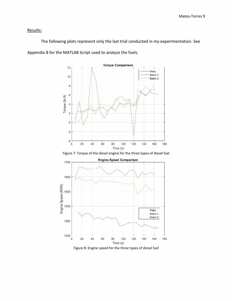
The following plots represent only the last trial conducted in my experimentation. See

Appendix B for the MATLAB Script used to analyze the fuels.

Figure 7: Torque of the diesel engine for the three types of diesel fuel

Figure 8: Engine speed for the three types of diesel fuel

Matos-Torres 10

Figure 9: Scatter plot of the torque versus engine speed for the three types of diesel fuel

Figure 10: Fuel flow for each of the three types of diesel fuel

Matos-Torres 11

Figure 11: Air flow through the engine for each of the three diesel fuels

Figure 12: Fuel to Air ratio within the engine for each of the three diesel fuels

Matos-Torres 12

Discussion:

For all of the data analysis, “Batch 1” referred to the batch of biodiesel fuel I made and

“Batch 2” referred to the batch of biodiesel fuel the E14 group made. Only the last trial was

analyzed because accessing the data from previous trials was a challenge. When analyzing the

data, I realized I saved all of the data in three files, one for each fuel. Because of this, MATLAB

was only able to import the data for last trial in each file.

Figure 7 showed the engine had comparable torques for the petro diesel and both

batches of biodiesel when subjected to the same electrical load variation. Batch 1 had two large

spikes in torque during the trial that neither of the other two fuels had. I compared the torques

from my data to the torques in Jonathan Martin’s E90 and noticed he had some of the same

spikes in torque for his biodiesel fuel. He noted that this could be caused by the engine wobble.

Figure 8 showed the engine speed (RPM) with each of the fuels. The petro diesel and

Batch 2 had similar trends as the electrical load increased. The engine speed with these two

fuels decreased as the load increased, which was expected since the throttle remained constant

did not change during the trial. The petro diesel finished approximately 80 RPM slower than it

began. Batch 2 finished approximately 40 RPM slower than it began. Batch 1 was the oddball

when analyzing the engine speed. Batch 1 actually had a large increase in engine speed at the

beginning of the trial relative to the other two fuels. The engine speed oscillated a noticeable

amount with Batch 1 and even finished the trial approximately 15-20 RPM higher than it began,

which should not have happened. Because the other trials were not analyzed, I am uncertain if

this is an anomaly or if Batch 1 displayed this behavior repeatedly.

Matos-Torres 13

Figure 9 compared the torque to the engine speed for each fuel. This comparison

unveiled a significant behavioral difference for the fuels. Even though the petro diesel had the

largest total change in RPM, the torque was more consistent and tightly grouped in the scatter

plot. Both batches of biodiesel had erratic torque behavior when compared to the engine

speed. The spikes in torque noticed in Figure 7 for Batch 1 played a role in the erratic behavior

shown in Figure 9. Differences in the chemical composition of the biodiesel batches may have

contributed to this erratic behavior.

Figure 10 recorded the fuel flow for each of the fuels. It appeared that the boat was

stuck during the petro diesel trial and I did not notice it at the time. Because of this, the fuel

flow and fuel to air ratio for the petro diesel were irrelevant. Batch 1 and Batch 2 provided

useful fuel flow data, though. The data showed an increase in fuel flow as the electrical load

increased. Batch 2 had several large oscillations in its fuel flow. Chemical differences, such as

viscosity, combustion temperature, and composition may have contributed to the differences in

fuel flow. During a visual comparison of the two batches, I observed that Batch 1 was a lot

brighter in color and not as translucent as Batch 2. I noticed Batch 1 appeared to be more

viscous than Batch 2 due to how easily Batch 2 moved when the flasks were swirled.

Figure 11 compared the air flow recorded for each fuel. The air flows were comparable

in behavior for each fuel. Each oscillated similarly, but the petro diesel had lower minimum air

flow values, which may have been since the petro diesel ran at a lower engine speed than the

two batches of biodiesel.

Figure 12 compared the fuel to air ratio for each fuel. At first glance, the batches of

biodiesel appeared to have significantly different fuel to air ratios. If you exclude the time

Matos-Torres 14

intervals where Batch 2 had large spikes in fuel flow in Figure 10, Batch 1 and Batch 2 had very

similar fuel to air ratios. The plot of the ratios even had similar oscillation shapes, which meant

the engine reacted to the varying electrical load in comparable ways with both batches of

biodiesel.

Whenever I expand this project for my E90 next year, I would do several things

differently. To reduce the possibility of the boat getting stuck during a trial, I would clean the

fuel tanks to remove any accumulation of fuel stuck to the walls and bottom. Afterwards, I

would recalibrate all of the transducers and the orifice meter since this project assumed all of

Jonathan’s calibrations from 2012 were still accurate four years later. I would personally make

all of the biodiesel fuel to ensure the same procedures were used. One piece of equipment to

invest in would be a separatory funnel to simplify the decanting process. Expanding this project

would mean doing mass spectrometry and/or gas chromatography to chemically compare

petro diesel and the batches of biodiesel fuel. Another aspect I want to incorporate is filtration

of waste vegetable oil to chemically compare the filtered oil to virgin vegetable oil and

determine the best method of treating the filtered oil when producing biodiesel fuel.

Conclusion:

The purpose of this project was to recreate aspects of the E90 project Jonathan Martin

’12 did and determine if there was a significant performance difference when using biodiesel

fuel instead of petro diesel. Data was collected by running the diesel test stand with petro

diesel and two batches of biodiesel fuel. There appeared to be slight performance differences in

the limited torque, engine speed, fuel flow, and air flow data analyzed.

Matos-Torres 15

Works Cited

"American Fuels." U.S. On-Highway Diesel Fuel Consumption. Mike Gregory, 9 Apr. 2014. Web.

13 May 2016. <http://www.americanfuels.net/2014/04/us-on-highway-diesel-fuel-

consumption.html>.

"Learn About Biodiesel." US Environmental Protection Agency. N.p., 27 Apr. 2016. Web. 14 May

2016. <https://www3.epa.gov/region9/waste/biodiesel/questions.html>.

"Petroleum Consumption - World Statistics and Charts as Map, Diagram and Table." Petroleum

Consumption / Countries of the World. N.p., 18 Jan. 2016. Web. 13 May 2016.

<http://world.bymap.org/OilConsumption.html>.

Matos-Torres 16

Appendix A: DieselDAQ.m

%% DieselDAQ.m

% Reads data from diesel engine test stand, outputs engine variables to txt

% file, plots variables.

%

% Based on significant contributions from the E90 project done by

% Jonathan Martin '12 and pieces of the oveneval.m script used by Steven

% Matos-Torres '17, Cole Fox '17, Graham Lesko '17, and Cooper Woolston '17

% for the E14 Oven Lab.

%% Set calibration values

clear;clf;

format compact;

% define coefficients

AirSlope = 0.478; % in. H20/mV; calculating airflow and pressure difference

FlowCoeff = 1.0456; % PPH*(diff. psi)'2; calculating airflow

WaterSlope = 9.992; % mL/s/Hz; calculating waterflow

FuelSlope = -32.48; % mL/V; calculating fuel flow

FuelEmpty = -4.836; % V @ 0 mL; voltage when fuel reservoir empty

TorqueSlope = 9.777; % lb-ft/mV; calculating engine torque

Torquelnt = -10.78; % lb-ft @ 0 mV; initial engine torque

%% Preallocate arrays for variables to be measured (for performance)

t1 = clock; % set clock

b=20; % number of elements in each array = total number of data points to be

taken

n=20; % number of snapshots taken for torque

ti=zeros(size(b)); % Time array

EngineSpeed=zeros(size(b)); % Engine Speed array

tachometer=zeros(size(b)); % Tachometer array

FuelLevel=zeros(size(b)); % Fuel Level array

WaterIn=zeros(size(b)); % Water In array

WaterOut=zeros(size(b)); % Water Out array

AirFlow=zeros(size(b)); % Air Flow array

WaterFlow=zeros(size(b)); % Water Flow array

TorqueSnap=zeros(size(b,n)); % b-by-n array holding snapshots of torque

EngineTorque=zeros(size(b)); % mean values of Torque for each b

%% Open link with Agilent DAQ board

% USB interface applies only to Keysight 34972A LXI Data Acquisition / Switch

% Unit. Use GPIB0 interface otherwise.

daq = visa('agilent','USB0::0x0957::0x2007::my49021465::0::INSTR');

fopen(daq);

% Get file info from user

filnam = input('Name of file to hold data: ','s');

fid = fopen(filnam, 'at');

%% Thermocouple readings being set to variables

% Takes user input to name the data sequence

DSEQ=input('ENTER THE NAME OF THIS TEST: ','s');

% Prepare output file

fprintf(fid,'\n\n'); % insert two blank lines between current and previous

test

fprintf(fid,'%s', 'TEST=',DSEQ);

% create headings in command window and output txt file

fprintf(' %7s%7s%7s%7s%7s%7s%7s%7s%7s','Index','Time',...

'EngSpd','WtrIn','WtrOut','WtrFlw',...

'PrsDif','AirFlw','FuelLv');

fprintf(fid,'\n %7s%7s%7s%7s%7s%7s%7s%7s%7s','Index','Time',...

Matos-Torres 17

'EngSpd','WtrIn','WtrOut','WtrFlw',...

'PrsDif','AirFlw','FuelLv');

% Get inital fuel level and time measurements

fprintf(daq, 'MEAS:VOLT:DC? AUTO,(@108)\n');

FuelLevel(1) = (str2double(fscanf(daq))-FuelEmpty)*FuelSlope; % mL

for i=2:1:(b+1)

ti(i-1)=etime(clock,t1); % ti is the time in sec

% Tachometer (engine speed) readings

fprintf(daq, 'MEAS:FREQ? MIN,(@101)\n');

EngineSpeed(i-1) = 60/8*str2double(fscanf(daq)); % Engine speed - RPM60

Sec/Min, 8 Periods/Rotation

% Temperature readings

fprintf(daq, 'MEAS:TEMP? TC,K,(@104)\n');

WaterIn(i-1) = str2num(fscanf(daq)); % deg C

fprintf(daq, 'MEAS:TEMP? TC,K,(@105)\n');

WaterOut(i-1) = str2num(fscanf(daq)); % deg C

% Airflow readings from voltage


PressDiff = max([AirSlope*1000*str2num(fscanf(daq)),0]); % in. H20 must

be >= 0 or flow rate will be complex number

AirFlow(i-1) = sqrt(PressDiff*14.7)*FlowCoeff; % PPH

% Waterflow readings from voltage

fprintf(daq, 'MEAS:FREQ? AUTO,(@107)\n'); % mL/s

WaterFlow(i-1) = WaterSlope*str2double(fscanf(daq)); % mL/s

% Fuelflow readings from voltage


FuelLevel(i) = (str2num(fscanf(daq))-FuelEmpty)*FuelSlope; % mL

%Because of wobble in engine, torque must be measured many times

for x = 1:1:n


TorqueSnap(i-1,x) = str2num(fscanf(daq));

end

EngineTorque(i-1) = TorqueSlope*1000*mean(TorqueSnap(i-1,:))+Torquelnt;

% Print data in MATLAB window;

fprintf('\n %7.0f%7.0f%7.0f%7.1f%7.1f%7.1f%7.1f%7.1f%7.1f',i-1,ti(i-

1),...

EngineSpeed(i-1),WaterIn(i-1),WaterOut(i-1),WaterFlow(i-1),...

PressDiff,AirFlow(i-1),FuelLevel(i-1));

% Print data in output file;

fprintf(fid,'\n %7.0f%7.0f%7.0f%7.1f%7.1f%7.1f%7.1f%7.1f%7.1f',i-1,ti(i-

1),...

EngineSpeed(i-1),WaterIn(i-1),WaterOut(i-1),WaterFlow(i-1),...

PressDiff,AirFlow(i-1),FuelLevel(i-1));

%% Plot data

% plot engine speed

subplot(3,2,1)

plot(ti(1:end),EngineSpeed)

title('Engine Speed')

xlabel('sec elapsed')

Matos-Torres 18

ylabel( 'RPM' )

% plot waterin and waterout

subplot(3,2,2)

plot(ti(1:end),WaterIn,ti(1:end),WaterOut)

title('Temperatures')


ylabel('deg C')

legend('Water In','Water Out','Location','West')

legend('boxoff')

% plot airflow

subplot(3,2,3)

plot(ti(1:end),AirFlow)

title('Air Flow')


ylabel('PPH')

% plot waterflow

subplot(3,2,4)

plot(ti(1:end),WaterFlow)

title('Water Flow')


ylabel('mL/s')

% plot fuelflow (fuellevel)

subplot(3,2,5)

plot(ti(1:end),FuelLevel(2:end))

title('Fuel Flow')


ylabel('mL/s')

% plot engine torque

subplot(3,2,6)

plot(ti(1:end),EngineTorque)

title('Engine Torque')


ylabel('lb-ft')

pause(1)

end

% insert new line at the end of output

fprintf('\n');

fprintf(fid,'\n');

% save output as .mat file

filnam_save = strcat(filnam,'.mat');

save(filnam_save);

% close output txt file

fclose(fid);

fclose(daq); % close connection

delete(daq); % delete connection

Matos-Torres 19

Appendix B: DataAnalysis.m

%% Data Analysis

clc

%% Import Data files

petro = importdata('may3petro.mat');

batch1 = importdata('may3batch1.mat');

batch2 = importdata('may3batch2.mat');

%% Torque

T_p = petro.EngineTorque; % Torque for petrodiesel

T_1 = batch1.EngineTorque; % Torque for Batch 1

T_2 = batch2.EngineTorque; % Torque for Batch 2

figure(1)

plot(petro.ti,T_p)

hold on; grid on;

plot(batch1.ti,T_1);

plot(batch2.ti,T_2);

title('Torque Comparison')

xlabel('Time (s)'); ylabel('Torque (lb-ft)');

hold off;

legend('Petro','Batch 1','Batch 2','Location','Best')

%% Engine Speeed

s_p = petro.EngineSpeed; % RPM for petrodiesel

s_1 = batch1.EngineSpeed; % RPM for Batch 1

s_2 = batch2.EngineSpeed; % RPM for Batch 2

figure(2)

plot(petro.ti,s_p)

hold on; grid on;

plot(batch1.ti,s_1);

plot(batch2.ti,s_2);

title('Engine Speed Comparison')

xlabel('Time (s)'); ylabel('Engine Speed (RPM)');

hold off;


%% Torque vs. Speed

figure(3)

scatter(s_p,T_p,'filled')

hold on;

scatter(s_1,T_1,'filled')

scatter(s_2,T_2,'filled')

grid on;

xlabel('Engine Speed (RPM)'); ylabel('Torque (lb-ft)');

title('Torque vs Speed')

hold off;

%% Fuel Flow

fuel_p = petro.FuelLevel(2:end); % mL

fuel_1 = batch1.FuelLevel(2:end); % mL

fuel_2 = batch2.FuelLevel(2:end); % mL

% Calculate fuel flow in mL/s

ff_p(1) = (petro.FuelLevel(2)-petro.FuelLevel(1))/petro.ti(1);

ff_1(1) = (batch1.FuelLevel(2)-batch1.FuelLevel(1))/batch1.ti(1);

ff_2(1) = (batch2.FuelLevel(2)-batch2.FuelLevel(1))/batch2.ti(1);

for i=2:1:20

ff_p(i) = (fuel_p(i)-fuel_p(i-1))/(petro.ti(i)-petro.ti(i-1)); % mL/s

ff_1(i) = (fuel_1(i)-fuel_1(i-1))/(batch1.ti(i)-batch1.ti(i-1));

ff_2(i) = (fuel_2(i)-fuel_2(i-1))/(batch2.ti(i)-batch2.ti(i-1));

Matos-Torres 20

end

figure(4)

plot(petro.ti,ff_p);

hold on

plot(batch1.ti,ff_1)

plot(batch2.ti,ff_2)

hold off

xlabel('Time (s)'); ylabel('Fuel Flow (mL/s)')

title('Fuel Flow')


%% Air Flow

air_p = (petro.AirFlow); %lb/hr

air_1 = (batch1.AirFlow);

air_2 = (batch2.AirFlow);

figure(5)

plot(petro.ti,air_p)

hold on;

plot(batch1.ti,air_1)

plot(batch2.ti,air_2)

hold off

xlabel('Time(s)'); ylabel('Air Flow (lb/hour)');

title('Air Flow Comparison');


%% Fuel to Air Ratio

ratio_p = (3600.*ff_p./5.7)./air_p; % 3600 mL/hr = 5.7 lb/hr

ratio_1 = (3600.*ff_1./5.7)./air_1;

ratio_2 = (3600.*ff_2./5.7)./air_2;

figure(6)

plot(petro.ti,ratio_p)

hold on;

xlabel('Time (s)'); ylabel('lb Fuel/lb Air')

title('Fuel to Air Ratio')

plot(batch1.ti,ratio_1)

plot(batch2.ti,ratio_2)

hold off;


e81 final report

Documents