e ects of wind power intermittency on generation and emissions

E�ects of Wind Power Intermittency on Generation

and Emissions

Reid Dorsey-Palmateer∗

October 31, 2014

Abstract

The level of potential wind generation for a given set of turbines depends on wind

conditions which vary over time and are imperfectly forecastable. Because grid op-

erators must be prepared to compensate for expected or unexpected changes in wind

generation, this intermittency a�ects the operation of the electric grid and the result-

ing emissions. Using ERCOT and EPA data for Texas, this paper �nds that increased

wind generation shifts the mix of the remaining fossil fuel generation toward natural

gas generation, which has more �exible output levels than coal. Because natural gas

generation is cleaner than coal, this shift towards natural gas generation results in low-

ered emissions levels. This reduction in CO2 emissions in the ERCOT region has an

average annual value of approximately $65M from 2011 to 2013. However, this inter-

mittency e�ect on CO2 has shrunk substantially from 2011 to 2013 in Texas as short

run wind generation forecasts have become more accurate and as market participants

have obtained more experience with higher levels of wind generation. This e�ect is

also smaller during periods where natural gas generation would otherwise comprise a

relatively large portion of the fossil fuel generation mix. While wind intermittency does

a�ect the operation of the grid and the resulting cost of electricity, its environmental

bene�ts should also be accounted for when determining public policy towards wind

generation as the estimated environmental bene�ts can non-trivially reduce the overall

social cost of wind power intermittency.

∗University of Michigan. Email: [email protected]. Thanks to Ryan Kellogg, Shaun McRae, DanielAckerberg, Jeremy Fox, Tom Lyon, Catherine Hausman and seminar participants at the University of Michi-gan, Western Economics Association Annual Conference and Camp Resources for their feedback.

1

1 Introduction

Electricity generation is a major source of air pollution in the United States, responsible

for 32% of greenhouse gas emissions in 2012. Because wind power does not generate any

emissions, it has been promoted as a clean way to generate electricity, with a variety of

government policies encouraging its use. However, wind power di�ers from fossil fuel gen-

eration in another way: its dependence on wind conditions which vary over time and are

imperfectly forecastable. In the absence of storage technology, electricity generation must

be continuously matched with consumption, so this wind power intermittency can a�ect the

operation of the electricity grid.1

Wind generation reduces the required amount of generation from other sources so if wind

generation capacity is relatively small compared to the overall electric load, any expected or

unexpected variation in wind generation may not be substantial relative to the short-run vari-

ation in electricity load. However if wind generation capacity is relatively large and changes

in wind generation are compensated for by changing fossil fuel generation levels, greater wind

intermittency could increase the optimal desired �exibility of fossil fuel generation.2

Thus because of its intermittency, wind power is imposing an externality on the rest

of the electricity grid: other generators, and potentially the demand-side, must respond

to changes in wind generation. Paying for reserve power and otherwise operating the grid

in a less cost-minimizing manner imposes a �nancial cost. Recent engineering estimates

of these costs range from $2 to $6 per MWh of wind generation produced (Albadi and El-

Saadany [2010]).3 Beyond �nancial costs, wind power intermittency may have environmental

externalities that should be accounted for as well.

1Large scale storage of electricity is not currently feasible apart from hydropower. This paper examinesthe Texas market where hydropower is a very small part of the mix of generators.

2A 2008 report commissioned by ERCOT found that, for their model, when wind generation capacity inTexas was at 5000 MW, the wind generation would have �a limited impact on the system...[its] variabilitybarely rising above the inherent variability caused by system loads�. But when wind generation capacityincreased to 10,000 MW, �the impacts become more noticeable� and by 15,000 MW, �the operational issuesposed by wind generation will become a signi�cant focus of ERCOT operations� [GE Report, 2008].

3The engineering analysis in the Albadi and El-Saadany paper was not limited to Texas, in contrast withthis paper.

2

Wind power intermittency could a�ect the emissions produced by electricity generation.

Fossil fuel generators di�er with respect to their marginal costs, their ability to quickly adjust

output levels, as well as the pollution they produce. Compared to coal, natural gas generation

tends to be more expensive, less polluting and able to change output levels more rapidly. If

wind power intermittency shifts the mix of fossil fuel generation toward cleaner and more

�exible natural gas and away from coal, then this channel would reduce the pollution from

fossil fuel generation. However, e�ciency of individual generation units varies with output,

generally with higher e�ciency at higher output levels. If wind intermittency causes some

fossil fuel generators to be operated at lower output levels than would otherwise be the case,

this channel could increase their emissions rate (Bushnell and Wolfram [2005]). Furthermore,

when generator units are changing output levels, as would be the case when compensating

for wind power changes, they again lose e�ciency and increase their emissions rate (Novan

[forthcoming]).

Various government programs, such as the lapsed federal Production Tax Credit and

state-level renewable energy credits, have sought to increase the amount of wind genera-

tion.4,5 California, for example, has a goal of generating 33% of its electricity from renew-

able sources by 2020. Historically, the value of these wind generation subsidies have only

been linked to the quantity of power generated by turbines. If the purpose of subsidizing

wind power is to reduce emissions, this subsidy policy would optimally instead connect the

value of the externalities imposed by wind generation to the value of the subsidy.6,7 Varying

subsidy levels across wind turbines based on their e�ect on emissions could lead to improved

siting decisions (Novan [forthcoming]). If wind intermittency a�ects the operation of the

grid, subsidization policy would ideally incorporate wind generation intermittency and the

4While wind generation does not pollute in the conventional sense, nearby residents can complain aboutnoise and unsightly turbines.

5Hitaj (2013) and Carley (2009) examine the e�ectiveness of programs at encouraging wind generation.6Alternative polices such as cap-and-trade or a carbon tax could also be preferable to a subsidy for wind

generation, however this is beyond the scope of this paper.7The creation of �green jobs� has also been suggested as a rationale for subsidizing wind power (Obama

2012).

3

value of its corresponding externalities. This includes environmental externalities in addition

to imposed �nancial costs.

Other papers have looked at the integration of large quantities of intermittent generation

resources such as wind and solar into the electric grid (van Kooten [2010], DeCarolis and

Keith [2004], Gowrisankaran et al. [2014]).8 This set of papers uses 'engineering' approaches

and models the dispatch of generation units. This approach is valuable for out-of-sample

prediction but in practice the results from engineering models of electric grids can often

deviate from what is ultimately observed (Callaway and Fowlie [2009]).9

Instead of using a detailed dispatch model of the electricity grid, I use an instrumental

variables regression approach to estimate the impact of wind generation intermittency on

the operation of the electric grid and the resulting emissions. I use recent data from Texas,

the state with the most installed capacity for wind generation in the United States, from

approximately 2011 to 2013

In Texas, wind was the source of approximately 10% of electricity in 2013 and the share

of total generation coming from wind power at a speci�c moment has reached as high as 36%.

I obtain hourly data regarding emissions, fossil fuel generation and and both potential and

actual wind generation. I �nd that wind power does have an e�ect on electricity generation

beyond reducing the necessary amount of generation from other sources. After �exibly

controlling for the level of fossil fuel generation, increased wind generation is associated with

shifting the fossil fuel generation mix away from coal and towards more �exible natural gas

generation. There is also a corresponding decrease in CO2 emissions, indicating that the

environmental e�ect from shifting the generation mix towards cleaner natural gas dominates

any increase in emissions due to increased ramping of fossil fuel generators or operating at

less e�cient output levels.

This intermittency e�ect of wind generation on emissions is greater when natural gas

8Green and Vasilakos (2010) model how increased wind generation could a�ect market prices and outputwith pro�t maximizing bidding.

9In a di�erent context, Allcott and Greenstone (2012) discuss how engineering models of energy e�ciencyoften understate costs of improved energy e�ciency.

4

would otherwise comprise a smaller part of the generation mix, namely when total generation

is at lower levels and baseload coal generation is a larger part of the fossil fuel mix. While the

analysis in this paper only uses Texas data, this does suggest that wind power intermittency

may have a larger impact on generation and emissions in regions where coal generation plays

a larger role. This result is similar to Holland and Mansur (2008), who �nd that reducing

daily electricity load variation has di�erent e�ects on emissions depending on the generation

mix in the region.

Examining the average impact of wind power intermittency e�ect does not distinguish

between the di�erent forms that wind power intermittency can take. Wind generation levels

can vary in expected ways. Additionally, potential wind power could change in an unex-

pected manner if the forecasts are incorrect. These forecasts can have varying degrees of

con�dence. When examining the e�ect of more speci�c measures of wind intermittency,

I �nd that variation in expected wind generation over a �ve-hour window (expected wind

power variation) is associated with a shift in fossil fuel generation towards natural gas and a

decrease in CO2 emissions. This suggests that any e�ect on emissions of ramping fossil fuel

generation output to compensate for wind intermittency is dominated by the shifting fossil

fuel generation mix. I also �nd decreased precision in wind power forecasts results in shifts

from coal to natural gas and CO2 reductions as the level of wind generation increases.

The estimates in this paper are short-run e�ects that do not incorporate any long-run

adjustments to the set of generators available in Texas as a response to increased wind

generation capacity. Also, while total wind generation capacity did increase during the three

year period examined, a clear majority of the capacity was already installed in Texas at the

beginning of that three year period. Most of the observed variation in wind generation levels

is a result of changing wind conditions. The impact of installing additional wind turbines on

wind generation intermittency depends on how the new wind generation is correlated with

the previously installed capacity.

Thus while wind intermittency increases �nancial costs of generation, it also results in

5

reduced emissions by shifting fossil fuel generation towards cleaner natural gas generators.

When measuring the social cost wind intermittency imposes, the value of these environmental

bene�ts should be included. Using the estimates from Texas in this paper and the U.S.

social cost of carbon estimates of $39/ton, the environmental bene�t from increased wind

intermittency from a 1 MWh increase in wind generation is associated with a reduction in

CO2 emissions valued at $2.15.10 This value is generally smaller than engineering estimates

of the �nancial operating costs of wind intermittency, which can range from $2 to $6 per

MWh of wind power generated, but nevertheless indicates a substantial fraction of those

costs would be o�set by environmental bene�ts.

2 Modeling E�ects of Uncertain Wind Generation

To illustrate two channels of the e�ect of wind generation on the electrical grid and emis-

sions, I use a simpli�ed model of electricity generation. The planner must select a combi-

nation of generation sources to minimize costs with the constraint that the total generation

must equal the load. The quantity of electricity that needs to be supplied is imperfectly

forecast and the value of the load is distributed uniformly L ∼ U[(1 − γ)L̄, (1 + γ)L̄

].

Wind power is also imperfectly forecast and its value is also distributed uniformly W ∼

U[(1 − ν)W̄ , (1 + ν)W̄

].11,12 Uniform distributions are chosen for tractability. Wind gen-

eration has a per-MWh cost of zero.

Assume there are two other sources of power generation: coal and natural gas. Coal

and natural gas generation have per-MWh costs of cCoal and cNG respectively. Assume

cNG > cCoal. Additionally, let coal power have an in�exible output level that must be chosen

before the actual load and wind generation levels are determined. Natural gas generation is

adjustable and its output level can be selected after the load and wind generation levels are

10This does not include the value of any emissions reductions besides CO2.11Assume that ν and γ are between zero and one.12I abstract away from wind curtailment, or using less wind power than could be generated. In the context

of this model, however, wind curtailment would never be bene�cial.

6

known.

The lowest cost solution where W + qCoal + qNG = L is to set qCoal equal to the minimum

possible required generation, with the lowest realization of load and the highest realization

of wind generation. This is

qCoal = (1 − γ)L̄− (1 + ν)W̄

The amount of natural gas generation will be the quantity that is required to set total

generation equal to total load, taking qCoal as given:

qNG = L−W − (1 − γ)L̄+ (1 + ν)W̄

Increasing wind generation lowers the amount of natural gas generation.13 However,

increased forecast uncertainty (higher ν or γ) will lead to increased levels of natural gas

generation and lower amounts of coal. Because natural gas generation is more expensive and

cleaner than coal generation, this increased uncertainty will also lead to increased costs and

lower emissions levels. The relative value of these e�ects is unknown. This motivates the

empirical work in this paper, which estimates the e�ect of wind generation intermittency on

the use of coal and natural gas generation, along with the corresponding e�ect on emissions.

3 Background

The Electric Reliability Council of Texas (ERCOT) organizes the operation of the electricity

grid for about 75% of Texas, including 85% of the state's electric load. ERCOT's boundaries

are shown in Figure 1. Electricity generation can come from a variety of sources. Wind,

coal, nuclear and natural gas power are the dominant sources for ERCOT, comprising 99.2%

of total generation in 2013.14 With wind power accounting for 9.9% of generation in 2013,

ERCOT has the highest wind generation capacity of any U.S. state.

13In this simpli�ed model, when wind generation reduces the total fossil fuel generation, only coal gener-ation is lowered. In practice, this e�ect can reduce generation from both coal and natural gas power.

14The remaining electricity is generated mainly by hydropower, solar and biomass.

7

Wind generation capacity in Texas has grown quickly from near-zero levels in 2000,

though installation of additional wind generation capacity has slowed since 2009, as seen in

Figure 2.15 The actual quantity of wind power generated in ERCOT, dependent on installed

capacity, wind conditions and the ability of grid operators to dispatch the wind power, has

also grown over time, though less so since 2011, as seen in Figure 3. Wind generation

curtailment, where potential wind generation is not actually used, can occur and is mostly

due to transmission constraints between the western region of Texas containing most of the

wind generation capacity and the more populated regions. However, a long term project

to increase transmission capacity between these areas (CREZ) has substantially reduced

curtailment of wind power in recent years.

Additionally, while the electrical grid in the rest of the continental U.S. is more inter-

connected, ERCOT is relatively isolated with only a small number of connections to other

regions, as seen in Figure 4.16 This isolation allows electricity dispatch operations within

Texas to largely be conducted independently of the surrounding regions.

Under the current nodal system, instituted on November 1, 2010, ERCOT runs both day-

ahead and real-time markets for electricity. Because electricity cannot be economically stored

in large quantities, ERCOT identi�es the most cost-e�ective way to generate electricity to

match the expected load while respecting the system constraints, such as those imposed

by the transmission lines.17 ERCOT also obtains reserve power so generation capacity is

15Little wind generation capacity became active in 2013; this was likely due to the lapsing of the federalProduction Tax Credit (PTC) at the end of 2012. In order to qualify for that subsidy, wind turbines neededto be operational by the end of that year. Later legislation extended the PTC so that any turbine thathad begun construction by the end of 2013 would also qualify and additional turbines are expected to becompleted throughout 2014 and 2015.

16There are two DC connections to the Southwest Power Pool (SPP) with a combined capacity of 820MW and three DC connections to Mexico with a combined capacity of 286 MW. The DC connections allowcontrol over the �ow of power. Additionally two power plants can generate electricity simultaneously forboth ERCOT and an outside grid.

17For the day-ahead market, bids for both supply and demand of electricity for each hour of the next dayat speci�c locations may be submitted to ERCOT by 10 AM. Unit characteristics such as minimum andmaximum output levels must also be submitted. ERCOT releases the results of this auction by 1:30 PM. Thisstage of the market does not take ERCOT's forecasted load into account and allows �rms to reduce the pricerisk of transacting power in the real-time market. The next stage, day-ahead reliability unit commitment,occurs at 2:30 PM and does take forecasted load into account. ERCOT modi�es expected generator outputfor all hours of the next day so that planned generation will meet expected load at least cost while respecting

8

available to either increase or decrease generation quickly in response to unexpected changes.

Wind generation units participate with the other generator types in the wholesale elec-

tricity markets run by ERCOT. Because wind power does not consume any fuel and is very

inexpensive to operate once built, these wind units generally, though not always, submit

very low bids and are dispatched whenever possible, given constraints on the electric grid.18

There are di�erences in their treatment because of the intermittent nature of wind power.

Penalties for deviating from the requested output are relaxed for wind generation units so

that wind generation can �follow the wind�. Additionally, wind forecasts are critical in deter-

mining maximum potential generation in future periods. When operators of wind generation

units report their maximum potential output level for each upcoming hour in the day-ahead

and reliability unit commitment markets, this value cannot exceed ERCOT's forecast of

their potential wind generation. In the real-time market when dispatching wind turbines,

ERCOT uses a telemetered value based on current conditions at that generation site for the

maximum possible output for each wind generator instead of a value reported by the wind

unit operator.

An extensive discussion of the ERCOT market arrangements with respect to wind gen-

eration can be found in Sioshansi and Hurlbut (2010)

4 Data

Data for this project comes from ERCOT, the EPA, Weather Underground and the U.S.

Census. The analysis uses data from February 22, 2011 to December 31, 2013.19 Focusing

on this period avoids ERCOT's institutional shift from a zonal to a nodal market, which

constraints placed by the transmissions grid. This reliability unit commitment process is repeated hourlywith updated ERCOT forecasts and operating plans on the part of the generation units. Under normalcircumstances, the real-time market runs every �ve minutes. In the real-time market ERCOT adjusts therequested output from all generators based on changing conditions and does so to maintain system reliabilitywhile minimizing cost. As part of minimizing generation cost, ERCOT attempts to have the outcome of thereal time market minimize the use of regulation service, where ERCOT can request changes in output withinthree to �ve seconds to maintain appropriate frequency.

18Because of subsidies, wind generation units often submit bids with negative values.19I am missing data for some variables for a small number of days during this time period.

9

occurred on November 1, 2010 as well as large changes in the price of natural gas.

Generator output data comes from ERCOT. Generator output data from ERCOT's real-

time (SCED) market is available at 15 minute intervals and includes the quantity of electricity

generated by and the maximum potential output of each generation unit.20 The maximum

potential output levels for wind generation units at the time the generation units are dis-

patched depend on wind conditions and are telemetered data instead of being submitted by

the wind unit operators. Quantity of electricity generated only includes power added to the

grid and does not count any electricity consumed by the generator itself. This generation

data is often aggregated to the ERCOT-level for analysis.

Data on hourly CO2 emissions from power generation units are obtained through the

EPA's Continuous Emissions Monitoring System (CEMS). CEMS allows the EPA to track

compliance with emissions-related regulations.21 I use hourly emissions data for genera-

tion units within ERCOT and assume that all generation units that are a�ected by wind

generation in ERCOT are included.

A small number of natural gas units are missing CO2 data. I �ll in these missing values

using predicted values based on the heat rate, which is also available from CEMS.22 If valid

readings are not available, EPA requires that high emissions levels be recorded as a penalty.

The Sandy Creek coal facility recorded very high and unchanging emissions rates for an

extended period of time that were clearly due to CEMS recording issues. The generation

and emissions from this unit have been dropped from the analysis.

I create a single hourly temperature measure for Texas using a population-weighted

average of the 10 largest cities in ERCOT. Historical temperature data for these cities was

20This is called the High Sustainable Limit and assumes unlimited time to reach that speed. In practicethe amount of power that can be generated on short notice can be less than this maximum level.

21Generation units with a capacity less than 25 MW are not required to participate in CEMS and so thisanalysis omits emissions from those units.

22The R2 for the regression used in the prediction is about 0.95. Novan (Forthcoming) also uses the heatrate to approximate CO2 emissions for units with missing data.

10

obtained from the Weather Underground website.23,24 The city populations were taken from

the 2000 Census.

5 Wind Intermittency

Potential wind generation is dependent on actual wind conditions which changes over time.

Figure 5 illustrates how over one and �ve hours, the amount of potential wind power can

increase or decrease.25 For most initial potential wind generation levels, over a �ve-hour

horizon it is possible for almost all of the potential wind generation to be no longer available.

The magnitude of observed changes over a one hour horizon is substantially smaller, but

especially at the middle potential output levels, nontrivial decreases were observed. The

mean wind generation in Texas over this time period was 3467 MWh while the 75th percentile

was 5098 MWh. The di�erences in average change in variability at di�erent levels of wind

generation is likely due to correlation in output between wind generation units.26

In addition to forecasting upcoming levels of electric load, ERCOT forecasts future po-

tential wind generation. This forecast is used to help ensure the stability of the electric grid

by anticipating future changes in fossil fuel generation requirements and to allow ERCOT

to obtain those generation requirements in a low-cost manner. Furthermore, as noted by an

ERCOT representative, �with the increased percentage of the system load served by wind, it

becomes critical to have not only a good forecast of how wind will generate during the day,

but also an assessment of the level of uncertainty in that forecast.� (ERCOT Press Release,

2010). The short run wind forecasts used by ERCOT have improved substantially in recent

years. Figure 6 shows the distribution of one-hour-ahead potential wind generation forecast

23The airport associated with the city was the location of the data. Some cities share an airport and inthose cases the weight for that airport's temperature was the sum of the population of both cities.

24Some cities did not have historical temperature data for some hours. In these cases, the statewideweighted temperature measure was calculated without those cities.

25Potential wind generation is used instead of actual wind generation to exclude voluntary reduction ofwind power.

26Note that over longer time horizons, changes in wind generation could be due to the installation ofadditional wind turbines. Over a one or �ve hour period changes in potential wind generation will be dueto changing wind conditions.

11

errors. In all years from 2011-2013, the mean forecast error is near zero (-11.6 MWh in 2011,

-8.5 MWh in 2012 and 4.9 MWh in 2013). However, the average magnitude of the forecast

error has declined even as additional wind turbines have been installed and overall wind

generation levels increased, falling from 471.97 MWh in 2011 to 305.06 MWh in 2012 and

312.80 MWh in 2013.27

Because the generation must match total load, this wind intermittency will a�ect the

operations of the electric grid. An decrease in wind generation must be balanced by either

a decrease in electric load or an increase of electricity into the grid from another sources;

either some form of storage or through increased generation from fossil fuel generators. Large

scale battery storage is not �nancially feasible and Texas obtains a very small proportion

of its electricity come from hydropower, another form of electricity storage that Texas lacks

the necessary geography to e�ectively exploit.28 Demand response to maintain grid stability

is an alternative means of adjusting for changes in wind generation. While ERCOT has

worked to incorporate some load to be capable of quickly reducing their power consumption

in response to a signal, demand response has historically been used only several times per

year.29 Increased use of real-time pricing may also help, though having demand quickly

adjust to unforeseen changes in wind generation may not be as straightforward as adjusting

fossil fuel generation levels.

Adjusting the amount of fossil fuel generation in response to changes in wind generation

is an alternative. However, fossil fuel generators have di�erent abilities to adjust output

levels; natural gas is much more �exible, with the ramping rate of combined cycle natural

gas units generally about four times that of coal units (Tremath et al. [2013]). If it becomes

more optimal from either a cost minimization or grid stability perspective to have a more

�exible mix of fossil fuel generation sources, then this could result in a shift towards using

27Six hour ahead potential wind forecasts have not noticeably improved in terms of average magnitude offorecast error over these three years.

28In January 2013, a 36-MW battery project was completed, however this is not a substantial size giventhat the average wind generation in Texas is 3266 MWh.

29There were 21 uses of demand response between April 2006 and October 2011.

12

more natural gas to meet the same level of necessary fossil fuel generation.

Figure 7 shows the observed mix of hourly natural gas and coal generation at di�erent

levels of fossil fuel generation from Texas during the sample period. At any given level of

fossil fuel generation, there is a range of observed mixes of coal and natural gas generation.

Determining which mix to use in any given hour be based on a number of factors. Dynamic

considerations are one; if a given fossil fuel generation level occurs in the middle of the night,

that would likely result in a di�erent generation mix than if it occurred in late afternoon

because the latter would likely use more peaking generation. Plant maintenance is another, if

a coal facility is being repaired then this will likely result in increased natural gas generation

to compensate. If additional �exibility in fossil fuel output levels is preferred, this may also

result in shifting generation mix towards natural gas, as suggested in the stylized model from

Section 2.

While the wind power intermittency may result in a preference for more �exible fossil fuel

output levels to better adjust to future changes in potential wind generation, wind power also

directly o�sets fossil fuel generation requirements, as also seem in the model from Section

2. Figure 8 illustrates these di�erent e�ects: as the level of wind generation increases, the

level of fossil fuel falls, decreasing natural gas generation. If the desire for fossil fuel output

�exibility increases, however, the quantity of natural gas generation for a given level of total

fossil fuel generation increases.

5.1 Electricity Generation and Emissions

Electricity generation was responsible for 32% of greenhouse gas emissions in the United

States in 2012. While some generation sources such as wind, solar, geothermal or nuclear

power do not produce emissions, burning coal or natural gas does. Figure 9 shows hourly

SO2, CO2 and NOx emissions against hourly total electricity generation net of nuclear and

wind generation in ERCOT for the majority of 2011-2013.30 CO2 is the primary greenhouse

30In Texas, coal and natural gas power comprises almost all of the remaining generation.

13

gas associated with climate change. NOx is associated with the creation of ground-level ozone

and respiratory problems. SO2 emissions contribute to acid rain and respiratory problems.

Any e�ect of wind power on emissions will depend on how it a�ects the operation of the

grid. If the intermittent nature of wind power causes a shift in the fossil fuel mix towards

more �exible natural gas generation, then this could reduce emissions because natural gas

generating units are generally cleaner than coal units. Additionally, when total fossil fuel

generation is reduced in response to increased wind generation, the resulting reduction in

emissions will depend on what type of generation unit was o�set.31 Table 1 shows the average

emissions rates for coal plants, non-peaker natural gas plant and peaker natural gas plants in

the dataset.32 Because generators are more e�cient when operating at higher output levels,

Table 1 lists both overall average emissions rates and the average emissions rates conditional

on operating at high output levels. As seen in Table 1, the values are similar, suggesting

that the generating units are generally operated at e�cient levels.

Because peaker natural gas plants are those that are mainly used during peak conditions,

their average e�ciency is lower and emissions are higher than the more heavily used natural

gas plants. Compared to non-peaker natural gas units, on average, peaker natural gas units

emit 36% more CO2 per MWh, 224% more SO2 per MWh and over 700% more NOx per

MWh. Coal units generally have higher average emissions rates than natural gas units.

Natural gas units' average SO2 emissions rate are essentially nonexistent compared to coal

units' average SO2 emissions rate. The CO2 emissions rate for coal units is about twice that

of non-peaker natural gas and is 48% higher than peaker natural gas. Coal units also have a

NOx emissions rate about four times that of non-peaker natural gas, though peaker natural

gas does have a NOx emissions rate about twice that of coal.

If wind intermittency changes the fossil fuel generation mix, then this would likely impact

emissions. For a given level of fossil fuel generation, emissions would be expected to be higher

31Novan (forthcoming) �nds that increased wind generation results in larger emissions reductions whentotal generation levels are lower and coal is more likely to be the marginal unit.

32I de�ne a peaker natural gas plant as one whose observed generation is less than 15% of its potentialoutput.

14

when coal makes up a larger share of the fossil fuel generation. Additionally, generators are

less e�cient when they are changing output levels. When fossil fuel generators must ramp

their production levels up or down to compensate for changes in wind generation, this can

reduce the e�ciency of these generators and lead to increased emissions.The magnitude of

this impact as compared to shifting fossil fuel generation mix is an empirical question.

In addition to impacting emissions through intermittency, wind generation a�ects emis-

sions by reducing the total amount of fossil fuel generation. This e�ect results in a corre-

sponding decrease in emissions. Ka�ne et al. (2012) and Novan (forthcoming) �nd that the

e�ect of additional wind generation on emissions is related to the type of generation units

whose output is reduced by the wind power. Thus on average, if wind power reduces coal

power instead of non-peaker natural gas power, the e�ect of that increase of wind power on

emissions will on average di�er substantially.

The marginal generator can in turn depend on what the overall load is. Figure 7 shows

how on average the use of coal versus natural gas generation changes as the total fossil

fuel generation increases in Texas. Initially at low fossil fuel generation levels, additional

generation on average comes from both natural gas and coal generation. Once fossil fuel

generation is at about 30,000 MWh, further generation primarily comes from natural gas

plants, as can be seen by the essentially �at slope of the coal generation-net generation

relationship when net generation is high. Thus when total fossil fuel generation is high, the

e�ect of wind power on reducing total fossil fuel generation is likely to reduce natural gas

power.

6 Empirical Analysis

Using ERCOT-wide time series data, I examine how wind power intermittency a�ects the

fossil fuel generation mix and emissions. I initially test if wind generation has an e�ect on

electricity generation and emissions apart from simply reducing the amount of necessary

15

fossil fuel generation and �nd this is the case. I then test if this additional e�ect changes in

di�erent situations, across electric load levels and across years, before testing the e�ect of

explicit wind intermittency variables.

6.1 Baseline Model

To observe the e�ect of wind intermittency, my baseline model estimates the average e�ect of

additional wind generation on the fossil fuel generation mix and emissions while controlling

for the e�ect of wind generation on reducing total fossil fuel generation using the following

speci�cation:

DependentV art =β1Wt + f(FossilFuelt)+

α0 + α1Tempt + α2Temp2t + γmHourMontht + εt (1)

DependentV art is either the amount of natural gas generation or CO2 emissions in

hour t.33 Both the fossil fuel generation mix and the emissions will be a�ected by the

total amount of fossil fuel generation as seen in Figure 7. This is captured through the

f(FossilFuelt) term, a �fth-degree orthogonalized polynomial.34 The amount of required

fossil fuel generation is total required electricity generation net of generation from other fuel

sources. The amount of total electricity demand is assumed to be exogenous. Power must

then be generated to meet this in�exible load. For the state of Texas, this mainly comes

from nuclear, fossil fuel and wind power.35 Nuclear power reduces the amount of fossil fuel

generation, but these generation levels do not substantially change in the short term and

are also taken to be exogenous. Wind power also reduces the required amount of fossil fuel

33Note that because I control for the total level of fossil fuel generation, increasing the amount of naturalgas generation is increasing the share of natural gas generation in the fossil fuel generation mix. These resultsare robust to directly using the share of natural gas in fossil fuel generation as the dependent variable, asshown in Appendix A.

34Results are robust to using alternative degrees.35Other power sources such as biomass, solar and hydroelectric comprise less than 1% of the generation.

16

generation, as illustrated in Figure 8.36

The amount of wind power generated in hour t, Wt, reduces the amount of fossil fuel

generation, as illustrated in Figure 8 and this e�ect is captured in f(FossilFuelt). Wind

generation is allowed to have an additional e�ect, captured by β1. Identifying these e�ects

separately comes from variation in the total electric load as the wind power e�ect on total

fossil fuel generation is set to have the opposite e�ect as total electric load. If β1 is not equal

to zero, then wind generation has an additional e�ect on the dependent variables apart

from simply reducing the quantity of generation required from other sources. Considering

that, unlike conventional generation sources, wind power is not perfectly dispatchable and

depends on wind conditions, I will initially attribute this e�ect to wind intermittency. Later

speci�cations will include speci�c intermittency related variables.37

Temperature a�ects the e�ciency of generators and their resulting emissions, with high

temperatures reducing e�ciency. Furthermore, heterogeneous e�ects of temperature on e�-

ciency across generator types could a�ect the fossil fuel generation mix.

HourMontht is an hourly dummy variable that varies by year-month combination m,

included to address dynamic issues. Figure 10 plots the average total generation and wind

generation for each hour. The top panel shows that the average need for fossil fuel generation

can change across the hours of the day.38 For the same level of total fossil fuel generation,

baseload generators (those with lower marginal costs and less �exibility) should be a larger

share of the fossil fuel generation when the total required fossil fuel generation is near a local

36I assume that wind conditions do not a�ect the total load. Novan (forthcoming) notes that most windgeneration resources are located in a di�erent area of Texas as most electricity demand. Novan further notesthat the windspeed conditions on the ground are not highly correlated with windspeed conditions at theheight of the wind turbine blades.

37If β1 does represent the e�ect of wind power intermittency, then nuclear power (which does not produceemissions and whose production is not dependent on weather conditions) should not have an additionale�ect on the dependent variables apart from its role in reducing reducing fossil fuel generation. I separatelyrun this test and as expected �nd no signi�cant e�ect for nuclear power apart from reducing fossil fuelgeneration. However, the standard errors for the additional e�ect of nuclear power are several times largerthan the standard errors for the equivalent wind parameter. This is likely because of limited variation intotal nuclear generation levels, mainly driven by large jumps several times per year as opposed to substantialwithin-day variation as with wind.

38Total generation in Figure 10 includes nuclear power, however this does not vary substantially acrosshours.

17

minimum as compared to when it is near a local maximum; hourly controls are included to

address this. Because both average total generation and average wind generation are related

to the hour and this relationship can di�er across months, as seen in the lower two panels

of Figure 10, I also allow the hourly �xed e�ects to vary across months. This speci�cation

will also control for movement in relative fuel prices across months.

The amount of wind generation may not be exogenous. While wind speed likely is exoge-

nous, actual wind generation can be less than the maximum level allowed if grid operators

choose. This curtailment could happen for a number of reasons, most prominently trans-

mission constraints. To address endogeneity issues with wind curtailment, I instrument for

ERCOT-wide wind generation using the maximum possible generation (high sustainable

limit) given current conditions for all wind generation units. This is the expected maxi-

mum potential output of wind power used by ERCOT when dispatching wind generation

resources.39,40 Note that actual wind generation is on average quite close to the high sustain-

able limit and wind curtailment drops substantially from 2011 to 2013. Appendix B tests the

importance of using an instrument for the potentially endogenous wind generation variable

and �nds only minor di�erences.

To correct standard errors for heteroskedasticity and serial correlation, Newey-West stan-

dard errors with 69 lags are used. The lag order was determined through the automatic

bandwidth selection procedure of Newey and West (1994).41

After examining the impact of wind power intermittency on the fossil fuel generation

mix, I directly test the e�ect on aggregate CO2 emissions instead of using the generation

mix shifting result and measures of average emissions across the generator types. This is

because, as noted by Ka�ne et al. (2012) and Novan (forthcoming), emissions for a given

unit or type of unit is not always at its average level and directly estimating the e�ect of

39The maximum possible wind generation values in the real-time market are set by ERCOT based ontelemetered values, not on reported values from the operator of the wind generation resource. However,maintenance decisions for wind turbines could be endogenous.

40This di�ers from Novan (forthcoming) who uses a measure of wind speed as an instrument.41This is also close to the 3 days worth of lags used in Ka�ne et. al. (2012) when studying CO2 emissions

in ERCOT.

18

wind generation intermittency on emissions can account for these varying emissions levels.

See Ka�ne et al. (2012) or Novan (forthcoming) for a more complete discussion.

Table 2 shows selected results for this speci�cation. After accounting for its e�ect in

reducing fossil fuel generation, a 1 MWh increase in wind generation is associated with a

0.033 MWh shift in the fossil fuel generation mix away from coal and toward natural gas.

With this shift towards a cleaner fuel source, this wind intermittency e�ect from an increase

of 1 MWh of wind is associated with a reduction in 0.055 tons of CO2. Using a social cost

of carbon of $39/ton, this environmental bene�t from wind intermittency from an increase

of 1MWh of wind is valued at $2.15. With average wind generation of 3467 MW per hour,

this results in an average hourly reduction of 190.7 tons of CO2 and an annual value of over

$65 million.

6.2 Changes in E�ect Across Load and Time

While additional wind power shifts the fossil fuel generation mix towards natural gas, this

e�ect may be less prominent when natural gas is already a larger portion of the generation

mix. To test if this intermittency e�ect falls as load gets larger, I use the following speci-

�cation which allows for a di�erent impact depending on if total generation net of nuclear

power is relatively high or low:

DependentV art =β1Wt ∗ 1[High Loadt]+

β2Wt ∗ 1[Low Loadt]+

β31[High Loadt]+

f(FossilFuelt)+


where the cuto� for the high or low load indicator function is having total generation net

19

of nuclear power above or below 30,000 MWh, approximately its mean. When generation

net of nuclear power is this high, generally there is already a larger share of natural gas

generation, as seen in Figure 7. Table 3 shows the point estimate of the wind intermittency

e�ect on shifting fossil fuel generation from coal to natural gas is weaker when total generation

net of nuclear power is greater than 30,000 MWh, falling from 0.048 MWh to 0.028 MWh.

Similarly, the e�ect on reducing CO2 levels is weaker as well, falling from 0.072 tons of CO2

to 0.052 tons of CO2.42

To test if the intermittency e�ect changes over time, potentially as experience is gained

with relatively high levels of wind penetration and wind forecast precision increases, I allow

it to di�er across years as follows:

DependentV art =β1Wt ∗ 1[year = 2011]t+

β2Wt ∗ 1[year = 2012]t+

β3Wt ∗ 1[year = 2013]t+

f(FossilFuelt)+


Coe�cient estimates can be found in Table 4. The wind intermittency e�ect on shifting

fossil fuel generation from coal to natural gas is strongest in 2011, as is its impact on CO2

emissions. A 1 MWh increase in wind generation is associate of a shift in fossil fuel generation

from coal to natural gas of 0.075 MWh and a fall in CO2 emissions of 0.11 tons. By 2013, the

same 1 MWh increase in wind generation was responsible for a shift in fossil fuel generation

from coal to natural gas of 0.021 and a fall in CO2 emissions of 0.035.43 To the extent

42The di�erences in impact across generation levels on both CO2 emissions and shifting fossil fuel gener-ation to natural gas are statistically signi�cant at least at the 10% level.

43The estimated 2013 e�ect on natural gas generation is not statistically di�erent from zero. The di�erencein the e�ect on coal generation between 2011 and 2012 is signi�cant at the 10% level, the di�erence between2011 and 2013 has a p-value of 0.11. The di�erence in intermittency e�ect on CO2 generation between 2011and both of the following years is signi�cant at the 1% level.

20

that wind forecast precision from 2011 to later, as seen in Figure 6, any given level of

wind generation may be associated with lower risk of unexpected change in wind generation

in the later years, potentially contributing to the intermittency e�ect in 2011, β1, being

substantially larger than the other β parameters.

6.3 Explicit Intermittency Variables

In previous speci�cations, the e�ect of additional wind beyond reducing fossil fuel generation

has been interpreted as the e�ect of wind intermittency without indicating what feature

or features of wind generation was causing such e�ects, such as forecasted or unforecasted

change in wind generation. Identifying the speci�c features of wind intermittency responsible

for e�ects on fossil fuel generation mix and emissions will be important if the value of

wind intermittency is to be incorporated into policy decisions. I add a set of explicit wind

intermittency variables to do so:

DependentV art =β1Wt+

ψ[IntermittencyV arst]+

f(FossilFuelt)+


where IntermittencyVars are a vector of intermittency related variables that vary across

speci�cations.

To capture the e�ect of expected changes in wind generation over time, I calculate the

standard deviation of wind generation over a �ve hour window spanning two hours before

and after hour t ; for the upcoming two hours I use forecasted potential wind generation for

those hours in hour t to distinguish between expected and unexpected change.

To capture the e�ect of uncertainty in wind power forecasts, ideally I would have a direct

21

measure of the uncertainty of the forecast. While ERCOT's potential wind power forecasts

do contain a probability distribution of outcomes, I do not observe this. Instead I note that

more uncertain forecasts would, on average, have error of larger magnitude. I also note that

the magnitude of percent forecast error is strongly correlated over short time horizons.44

For my measure of wind uncertainty in wind power forecasts I use the mean magnitude of

percent wind forecast error for the hours before and after hour t. In some speci�cations, I

interact this variable with wind generation because the e�ect of wind forecast uncertainty

may change with the level of wind generation. This variable measures wind power forecast

uncertainty with error and thus estimated coe�cients will be attenuated.

Five speci�cations are used with di�ering vectors of intermittency variables as follows:

1. No intermittency variables; reproduces results from equation 1 for ease of comparison

2. Standard deviation of expected wind generation (expected variation)

3. Mean magnitude of wind power forecast error (forecast uncertainty)

4. Mean magnitude of wind power forecast error (forecast uncertainty); mean magnitude

of wind power forecast error interacted with wind generation (forecast uncertainty

interacted with wind)

5. Standard deviation of expected wind generation (expected variation); mean magnitude

of wind power forecast error (forecast uncertainty); mean magnitude of wind power

forecast error interacted with wind generation (forecast uncertainty interacted with

wind)

Tables 5 and 6 show the coe�cient estimates for these speci�cations for natural gas generation

and CO2 emissions, respectively. Column 1 in both tables reproduces the results from

Table 2. When the measure of expected variation, the standard deviation of expected wind

44When calculating wind forecast error, I use the di�erence between one-hour ahead forecasts from theprior hour and the actual level of high sustainable limit wind generation in hour t as to not include windcurtailment in forecast error.

22

generation over a �ve hour window, is included, it shifts fossil fuel generation from coal to

natural gas and results in a decrease in CO2 emissions. Column 3 shows the e�ect of the

mean magnitude of wind power forecast error over the prior and upcoming hours. When

this e�ect is assumed to be constant, it is not statistically di�erent from zero in either its

e�ect on natural gas generation or CO2 emissions. When the e�ect of this measure of wind

power forecast uncertainty is allowed to vary with wind generation levels, as in column 4,

for both natural gas generation and CO2 emissions, this interaction term is statistically

signi�cant. Increased wind forecast uncertainty has a stronger e�ect on shifting additional

coal generation to natural gas and lowering CO2 when wind generation is higher. This is

consistent with wind power not being a major issue for grid management when the amount

of wind generation is small.

Column 5 includes all three variables (the standard deviation of expected wind generation

over a �ve hour window, the measure of wind forecast uncertainty and the measure of wind

forecast uncertainty interacted with wind generation). The e�ects of all three intermittency

variables remain qualitatively the same although the e�ect of each individual variable is not

as strong as it was when the others were not included. With an average standard deviation

of expected wind generation over a �ve hour window, this measure of expected wind variance

is responsible for an average reduction in CO2 emissions of 45.5 tons/hour. Using a social

cost of carbon of $39/ton, this is valued at $15.5 million per year. Using the average values

for wind generation and the average percentage magnitude of the wind forecast error, the

measure of wind forecast uncertainty is responsible for an average hourly reduction of 28.5

tons of CO2, valued at $9.7 million per year.

Both of these variables that capture expected wind power variation and wind power

forecast uncertainty are measured with error and are subject to attenuation bias. After

controlling for wind power's e�ect on fossil fuel generation, additional wind generation still

is associated with a reduction in CO2 even when the included intermittency variables from

column 5 are set to zero (although this e�ect is reduced from column 1 where there were

23

no explicit intermittency variables). This e�ect may be related to wind intermittency not

captured by my two measures.

7 Conclusion

Wind power intermittency imposes a �nancial cost on electricity generation. However this

intermittency also provides an environmental bene�t which should also be accounted for

when determining the social impacts of wind generation. On average, wind generation in-

termittency is associated with increased natural gas generation and reduced coal power.

Because natural gas generation is cleaner than coal generation, this intermittency-induced

shift reduces the emissions resulting from electricity generation. This e�ect dominates any

generator-level increased ine�ciency due to ramping production levels to accommodate wind

intermittency.

Using the U.S. social cost of carbon of $39/ton, the average e�ect of wind intermittency

from a 1 MWh increase in wind generation is associated with a reduction in CO2 emissions

valued at $2.15, not including the value of any emissions reductions apart from CO2. This

value is smaller than engineering estimates of the �nancial costs of wind intermittency of

around $2 to $6 per MWh of wind generation but nevertheless indicates a substantial fraction

of those �nancial costs would be o�set by environmental bene�ts, adding up to an average

of $65 million per year. If the social cost of carbon is underestimated due to unmeasurable

e�ects, as suggested by the IPCC (2007) report, then these environmental bene�ts from wind

intermittency will be understated as well.

The impact of intermittency on emissions reduction is relevant for subsidy policy. While

subsidizing each MWh of wind power based on its associated emissions reduction would be

ideal, this is not a practical solution. However, connecting the subsidy payments for each

wind turbine in part to its expected or actual contribution to total wind power intermittency

could be feasible; an additional wind turbine will contribute to the overall variation in wind

24

generation based on how its output is correlated with other wind turbines. Incorporating

this when setting subsidy levels would encourage any e�ect on variation in wind generation

to be incorporated into siting decisions for new wind turbines and more accurately align the

impact of additional wind turbines on emissions with the subsidy payment. Similarly, any

subsidy payment related to wind intermittency could re�ect the fossil fuel generation mix in

the region. While it may be bene�cial to lock in a methodology to calculate subsidy payments

before turbine is built to simplify �nancing concerns (compared to other generation sources,

the cost of wind generation is e�ectively all up-front when building the turbine), changes in

the social cost of wind generation intermittency over time would ideally be incorporated as

well. Most signi�cantly, when determining the social costs of wind intermittency, the impact

of intermittency on both generation costs and emissions reduction should be considered.

25

References

[1] Albadi, M.H., E.F. El-Saadany. �Overview of wind power intermittency impacts on

power systems� Electric Power Systems Research, 80 (2010) 627-632

[2] Allcott, Hunt and Michael Greenstone, "Is There an Energy E�ciency Gap?" Journal

of Economic Perspectives, 26(1) (2012) 3-28.

[3] Bushnell, James B. and Catherine Wolfram, "Ownership Change, Incentives and Plant

E�ciency: The Divestiture of U.S. Electric Generation Plants." CSEM-140. University

of California Energy Institute, March 2005

[4] Callaway, Duncan and Meridith Fowlie. �Greenhouse Gas Emissions Reductions from

Wind Energy: Location, Location, Location?� Working Paper. June 2009

[5] Carley, Sanya. �State renewable energy electricity policies: An empirical evaluation of

e�ectiveness� Energy Policy 37 (2009) 3071�3081

[6] Cullen, Joseph, �Measuring the Environmental Bene�ts of Wind Generated Electricity.�

American Economic Journal: Economic Policy (forthcoming)

[7] DeCarolis, Joseph and David Keith. "The economics of large-scale wind power in a

carbon constrained world" Energy Journal 34(4) (2004): 395-410.

[8] ERCOT Press Release, �ERCOT Using New Forecasting Tool to

Prepare for Wind Variability�. March 25, 2010. Retrieved from

http://www.ercot.com/news/press_releases/show/326

[9] General Electric. �Analysis of Wind Generation Impact on Ancilliary Services Require-

ments.� 2008

[10] Gowrisankaran, Gautam, Stanley Reynolds and Mario Samano. �Intermittency and the

Value of Renewable Energy�, NBER Working Paper No. 17086, 2014

26

[11] Green, Richard and Nicholas Vasilakos. �Market behaviour with large amounts of inter-

mittent generation.� Energy Policy 38 (2010) 3211�3220

[12] Hitaj, Claudia. �Wind Power Development in the United States�, Journal of Environ-

mental Economics and Management, 65 (2013): 394-410

[13] Holland, Stephen and Erin Mansur. �Is Real-Time Pricing Green?: The Environmental

Impacts of Electricity Demand Variance.� Review of Economics and Statistics 90(3)

(2008): 550-561

[14] Intergovernmental Panel on Climate Change. 2007. �Cli-

mate Change 2007: Synthesis Report� Retrieved from:

http://www.ipcc.ch/publications_and_data/publications_ipcc_fourth_assessment

_report_synthesis_report.htm

[15] Ka�ne, Daniel, Brannin McBee, and Jozef Lieskovsky. �Emissions Savings from Wind

Power Generation: Evidence from Texas, California, and the Upper Midwest.� Working

Paper (2012)

[16] Newey, Whitney and Kenneth West. �Automatic Lag Selection in Covariance Matrix

Estimation� Review of Economic Studies (1994) 61: 631-653

[17] Novan, Kevin. "Valuing the Wind: Renewable Energy Policies and Air Pollution

Avoided." American Economic Journal: Economic Policy (forthcoming).

[18] Obama, Barack. 2012. �State of the Union Address, 2012�. Retrieved from

http://www.whitehouse.gov/the-press-o�ce/2012/01/24/remarks-president-state-

union-address

[19] Sioshansi, Ramteen and David Hurlbut. �Market protocols in ERCOT and their e�ect

on wind generation.� Energy Policy 38 (2010) 3192�3197

27

[20] Tremath, Alex, Max Luke, Michael Shellenburger and Ted Nordhaus. �Coal Killer: How

Natural Gas Fuels the Clean Energy Revolution� Breakthrough Institute Publication

(2013)

[21] van Kooten, G. Cornelis. �Wind power: the economic impact of intermittency� Letters

in Spatial and Resource Sciences (2010) 3: 1�17

28

Figure 1

The ERCOT Region

Source: http://www.opuc.texas.gov/

29

Figure 2

Source: EIA

30

Figure 3

31

Figure 4

Source: http://www.opuc.texas.gov/

32

Figure 5

33

Figure 6

Potential wind generation forecast error is capped at 2000 MWh

34

Figure 7

35

Figure 8

36

Figure 9

37

Figure 10

38

Table 1

Coal Nonpeaker Natural Gas Peaker Natural Gas

SO2 lbs/Mwh 4.7925 0.0059 0.0191

CO2 tons/Mwh 1.0478 0.5232 0.7091

NOx lbs/Mwh 1.2346 0.2458 2.1581

SO2 lbs/Mwh at High Output 4.760 0.0053 0.0137

CO2 tons/Mwh at High Output 1.0408 0.4833 0.6755

NOx lbs/Mwh at High Output 1.2271 0.2289 2.0530

39

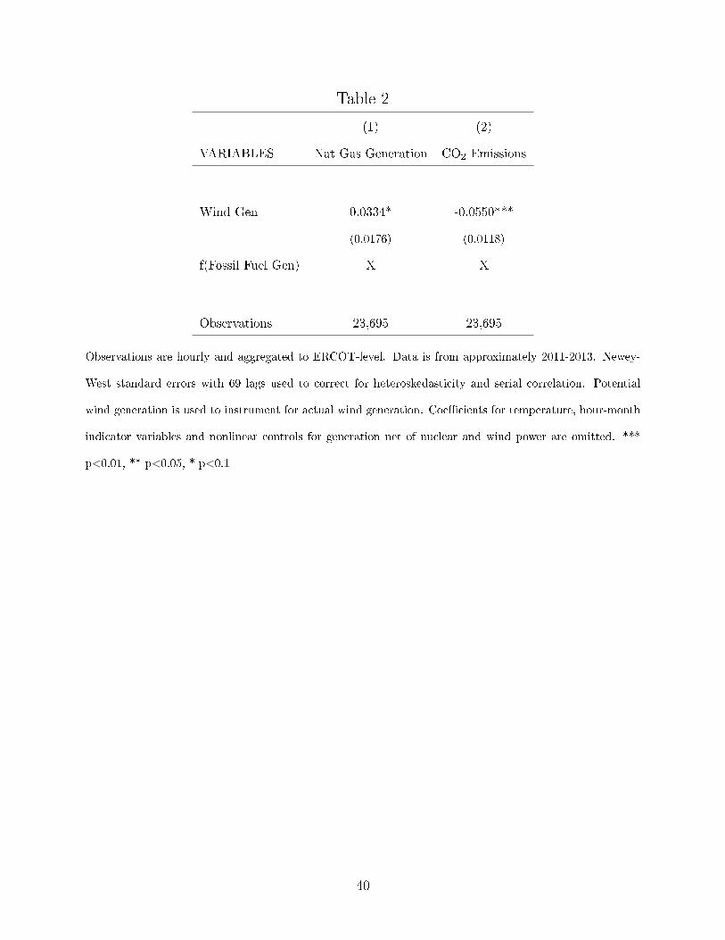
Table 2

(1) (2)

VARIABLES Nat Gas Generation CO2 Emissions

Wind Gen 0.0334* -0.0550***

(0.0176) (0.0118)

f(Fossil Fuel Gen) X X

Observations 23,695 23,695

Observations are hourly and aggregated to ERCOT-level. Data is from approximately 2011-2013. Newey-

West standard errors with 69 lags used to correct for heteroskedasticity and serial correlation. Potential

wind generation is used to instrument for actual wind generation. Coe�cients for temperature, hour-month

indicator variables and nonlinear controls for generation net of nuclear and wind power are omitted. ***

p<0.01, ** p<0.05, * p<0.1

40

Table 3

(1) (2)

VARIABLES Nat Gas Generation CO2

Wind Gen (High Load) 0.0281 -0.0515***

(0.0178) (0.0122)

Wind Gen (Low Load) 0.0481** -0.0719***

(0.0188) (0.0127)

High Load Indicator 29.73 22.29

(58.72) (41.77)



Observations are hourly and aggregated to ERCOT-level. Data is from approximately 2011-2013. High load

cuto� is total generation net of nuclear power of 30,000 MWh; approximately the mean in the sample. Newey-




p<0.01, ** p<0.05, * p<0.1

41

Table 4

(1) (2)

VARIABLES Nat Gas Generation CO2

Wind Gen (2011) 0.0747*** -0.107***

(0.0235) (0.0174)

Wind Gen (2012) 0.0217 -0.0444***

(0.0237) (0.0168)

Wind Gen (2013) 0.0206 -0.0348**

(0.0285) (0.0170)







p<0.01, ** p<0.05, * p<0.1

42

Table5

(1)

(2)

(3)

(4)

(5)

VARIABLES

NatGas

NatGas

NatGas

NatGas

NatGas

Generation

Generation

Generation

Generation

Generation

WindGen

0.0334*

0.0298*

0.0276

0.00841

0.00906

(0.0176)

(0.0176)

(0.0184)

(0.0213)

(0.0212)

Std

Dev

ofExpectedWindGen

(5HrWindow

)0.154***

0.131**

(0.0524)

(0.0511)

AvgPct

WindForecastError(2

HrWindow

)-225.9

-588.2**

-535.8**

(157.4)

(247.4)

(245.4)

WindGen

*AvgPct

WindForecastError(2

HrWindow

)0.201**

0.152*

(0.0825)

(0.0814)

f(FossilFuelGen)

XX

XX

X

Observations

23,695

23,695

23,695

23,695

23,695

Observationsare

hourlyandaggregatedto

ERCOT-level.Data

isfrom

approxim

ately

2011-2013.New

ey-W

eststandard

errors

with69lagsusedto

correctforheteroskedasticityandserial

correlation."AvgPct

WindForecast

Error(2

HrWindow

)"measureswindpow

erforecast

uncertainty."Std

Dev

ofExpectedWindGen

(5HrWindow

)"measuresexpectedvariance

inwindgeneration.Potentialwindgenerationisusedto

instrumentfor

actualwindgeneration.Coe�

cients

fortemperature,hour-month

indicatorvariablesandnonlinearcontrolsforgenerationnet

ofnuclearandwind

pow

erare

omitted.***p<0.01,**p<0.05,*p<0.1

43

Table6 (1)

(2)

(3)

(4)

(5)

VARIABLES

CO

2CO

2CO

2CO

2CO

2

WindGen

-0.0550***

-0.0519***

-0.0570***

-0.0433***

-0.0438***

(0.0118)

(0.0119)

(0.0122)

(0.0137)

(0.0136)

Std

Dev

ofExpectedWindGen

(5HrWindow

)-0.132***

-0.107***

(0.0385)

(0.0396)

AvgPct

WindForecastError(2

HrWindow

)-77.66

180.7

137.7

(109.4)

(167.1)

(166.6)

WindGen

*AvgPct

WindForecastError(2

HrWindow

)-0.143**

-0.103*

(0.0568)

(0.0573)

f(FossilFuelGen)

XX

XX

X

Observations

23,695

23,695

23,695

23,695

23,695

Observationsare


ERCOT-level.Data

isfrom

approxim

ately

2011-2013.New

ey-W

eststandard

errors

with69lagsusedto


correlation."AvgPct

WindForecast

Error(2

HrWindow

)"measureswindpow

erforecast

uncertainty."Std

Dev

ofExpectedWindGen

(5HrWindow



instrumentfor

actualwindgeneration.Coe�

cients



ofnuclearandwind

pow

erare

omitted.***p<0.01,**p<0.05,*p<0.1

44

Appendix A

The main text commonly uses the level of natural gas generation as a dependent variable.

In those speci�cations, I control for the total level of fossil fuel generation, implying that any

increase in natural gas generation increases the share of fossil fuel generation coming from

natural gas. I rerun the speci�cations based on equation 4 using the ratio of natural gas

generation to total fossil fuel generation as the dependent variable. Equation 4 is reproduced

here:

(Natural Gas Generation

Fossil Fuel Generation

)t

=β1Wt+

ψ[IntermittencyV arst]+

f(FossilFuelt)+

α0 + α1Tempt + α2Temp2t + γmHourMontht + εt

I run �ve speci�cations, with di�erent combinations of intermittency variables. These

are the same as in Section 6.3:

1. No intermittency variables; reproduces results from equation 1 for ease of comparison

2. Standard deviation of expected wind generation (expected variation)

3. Mean magnitude of wind power forecast error (forecast uncertainty)

4. Mean magnitude of wind power forecast error (forecast uncertainty); mean magnitude

of wind power forecast error interacted with wind generation (forecast uncertainty

interacted with wind)

5. Standard deviation of expected wind generation (expected variation); mean magnitude

of wind power forecast error (forecast uncertainty); mean magnitude of wind power

45

forecast error interacted with wind generation (forecast uncertainty interacted with

wind)

The coe�cient estimates can be found in Table A1. As compared to the earlier results

from Table 5 where the dependent variable was natural gas generation levels, all variables

that were statistically signi�cant earlier remain so. No variable that was not statistically

signi�cant in Table 5 is statistically signi�cant in Table A1. Additionally, the signs on all

coe�cients are the same across Tables 5 and A1.

46

TableA1

(1)

(2)

(3)

(4)

(5)

VARIA

BLES

NatGas-

NatGas-

NatGas-

NatGas-

NatGasto

FossilFuelRatio

FossilFuelRatio

FossilFuelRatio

FossilFuelRatio

FossilFuelRatio

WindGeneration

1.50e-06**

1.37e-06**

1.38e-06*

6.57e-07

6.79e-07

(6.77e-07)

(6.82e-07)

(7.16e-07)

(8.41e-07)

(8.38e-07)

Std

Dev

ofExpectedWindGen

(5HrWindow

)5.48e-06***

4.42e-06**

(2.04e-06)

(1.97e-06)

AvgPct

WindForecast

Error(2

HrWindow

)-0.00469

-0.0183**

-0.0166*

(0.00567)

(0.00868)

(0.00859)

WindGen

*AvgPct

WindForecast

Error(2

HrWindow

)7.55e-06**

5.91e-06*

(3.11e-06)

(3.04e-06)

f(FossilFuelGen)

XX

XX

X

Observations

23,695

23,695

23,695

23,695

23,695

"NatGas-

FossilFuel

Ratio"is

theratioofnaturalgasgenerationto

totalfossilfuel

generation.

Observationsare


ERCOT-level.Data

isfrom

approxim

ately

2011-2013.New

ey-W

eststandarderrors

with69lagsusedto


correlation."AvgPct

WindForecast

Error(2

HrWindow

)"measureswindpow

erforecast

uncertainty."Std

Dev

ofExpectedWindGen

(5Hr

Window



instrumentforactualwindgeneration.Coe�

cients



ofnuclearandwindpow

erare

omitted.***p<0.01,**

p<0.05,*p<0.1

47

Appendix B

While the weather conditions that determine the maximum potential wind generation are

exogenously determined, the actual level of wind generation is determined by a combina-

tion of windspeed conditions, supply and demand in the wholesale electricity market and

transmission constraints. Wind power can be curtailed by grid operators for a variety of

reasons; mainly to address congestion issues on transmission lines.The main analysis uses

the high sustainable limit of wind generation used by ERCOT in the dispatch process as an

instrument for actual wind generation. The actual wind generation is on average close to the

high sustainable limit, though this was less earlier in the period studied. Initially in 2011,

approximately 8% of potential wind power was curtailed. By 2013, additional transmission

capacity was introduced and average wind curtailment fell to under 2%.

To test the importance of using instrumental variables, I redo speci�cations 1 and 3,

reproduced here, without instrumentation.

DependentV art =β1Wt + f(FossilFuelt) + α0 + α1Tempt + α2Temp2t + γmHourMontht + εt

DependentV art =β1Wt ∗ 1[year = 2011]t + β2Wt ∗ 1[year = 2012]t + β3Wt ∗ 1[year = 2013]t+

f(FossilFuelt)+

α0 + α1Tempt + α2Temp2t + γmHourMontht + εt

Comparing the parameter estimates from Table B1 to Tables 2 and 4, instrumenting for

actual wind generation with potential wind generation does not result in substantial changes,

even for the e�ect of wind intermittency in 2011.

48

Table B1

(1) (2) (3) (4)

VARIABLES Nat Gas Gen CO2 Nat Gas Gen CO2

Wind Generation 0.0344* -0.0530***

(0.0178) (0.0118)

Wind Generation (2011) 0.0757*** -0.105***

(0.0235) (0.0174)

Wind Generation (2012) 0.0295 -0.0459***

(0.0230) (0.0167)

Wind Generation (2013) 0.0178 -0.0330*

(0.0287) (0.0170)

f(Fossil Fuel Gen) X X X X

Observations 23,695 23,695 23,695 23,695


West standard errors with 69 lags used to correct for heteroskedasticity and serial correlation. Coe�cients

for temperature, hour-month indicator variables and nonlinear controls for generation net of nuclear and

wind power are omitted. *** p<0.01, ** p<0.05, * p<0.1

49

e ects of wind power intermittency on generation and emissions

Documents