e ect of unsteady wind stress on the ekman layer

JOURNAL OF GEOPHYSICAL RESEARCH, VOL. ???, XXXX, DOI:10.1029/,

Effect of unsteady wind stress on the Ekman layer

Brian C. Barr , Donald N. Slinn

Department of Civil and Coastal Engineering, University of Florida

Gainesville, FL USA

Manhar R. Dhanak

Department of Ocean Engineering, Florida Atlantic University Boca Raton,

FL USA

Brian C. Barr , Donald N. Slinn, Department of Civil and Coastal Engineering, University of

Florida Gainesville, FL 32611-6590 ([email protected])

Manhar R. Dhanak Department of Ocean Engineering, Florida Atlantic University Boca Raton,

FL USA

X - 2 BARR ET AL.: UNSTEADY WIND STRESS AND THE EKMAN LAYER

Abstract. We investigate the role of an unsteady wind stress, both in

magnitude and direction, on a turbulent Ekman layer, using Large Eddy Sim-

ulations (LES). Analysis of the flow characteristics as well as the temporal

and spatial dependence of the eddy viscosity is presented, highlighting the

effect of the unsteadiness on modifying the depth of the Ekman layer. It has

previously been found that the tangential component of the Coriolis force,

often neglected in geophysical applications, is significant at influencing the

net properties of the Ekman layer, and can either increase or decrease the

mixed layer depth depending on the wind direction and latitude. The cur-

rent work suggests that the unsteady nature of wind on the ocean surface

will complicate separating the Ekman component of circulation from obser-

vations. The numerical method uses a pseudo-spectral Fourier technique for

the horizontal plane, and a finite difference discretization in the vertical di-

rection. The dynamic LES model is used for the subgrid closure. The domain

is periodic horizontally with an aspect ratio of 1 × 1 × 3.

BARR ET AL.: UNSTEADY WIND STRESS AND THE EKMAN LAYER X - 3

1. Introduction

In this paper, the effect of an unsteady wind stress on the ocean surface is investigated

with the help of large-eddy simulations (LES). Wind driven transport in the ocean has

been of interest since the landmark work of Ekman(1905).

Csanady (1967) notes that the Ekman layer is an example of a self-limiting boundary

layer. Given constant forcing, the Ekman layer will not grow infinitely deep (unlike a

boundary layer on an infinite flat plate).

Price et al. (1987) and Schudlich and Price (1998), using data from the LOTUS experi-

ment, see evidence of the Ekman spiral in their observations after using a ”wind relative”

averaging technique. While this technique greatly enhanced the signal to noise ratio of

their data for Ekman transport, this obfuscates the effect of wind direction on the Ekman

layer.

Zikanov, Slinn, and Dhanak (2003), hereafter referred to as ZSD03, conducted a thor-

ough study of the effect of including the full Coriolis force on the Ekman layer. They

concluded that depending on the wind direction, the tangential component of the Coriolis

force, often neglected by oceanographers, can act as either a source or a sink of turbulence.

Their simulations provided insight into the vertical distribution of the eddy viscosity, as

well as an elegant solution to the Ekman equations for a piecewise linear eddy viscosity

distribution.

Skyllingstad, Smyth and Crawford (2000) numerically investigate resonant wind driven

mixing in the upper mixed layer. Their model simulates effects of surface waves, Lang-


muir circulation, and buoyancy effects, while neglecting the tangential component of the

Coriolis force.

Important questions regarding the unsteady Ekman layer include:

1. How does varying the angle or amplitude of the wind change the Ekman layer prop-

erties (i.e. Ekman depth, angle of transport, and surface current)?

2. What is the time dependence of vertically varying eddy viscosity?

3. What it the response time of the Ekman layer to varied forcing?

4. Are there forcing conditions that can greatly enhance the depth of the Ekman layer?

5. What’s the simplest representation of the time dependent turbulent Ekman layer

that captures the essential physics of the problem?

The paper is organized as follows, §2 presents the problem formulation, equations, and

numerical method, §3 contains the results of the LES simulations, and finally §4 presents

concluding remarks.


2. Problem formulation

2.1. Simplifying assumptions

In order to focus on the implications of time-dependent wind-forcing of the Ekman

layer, a number of simplifying assumptions are made. First, the density is held to be a

constant. Stratification can act to limit the depth of the Ekman spiral; diurnal forcing

due to buoyancy fluxes will be held for future work. No other sources or sinks of energy

are present; this removes the effect of both Langmuir circulation and Stokes drift.

Viscous effects are ignored. Typical Reynolds numbers of oceanic flows are O(106). The

necessary domain size is O(100m). A direct numerical simulation (DNS) that resolves the

viscous dissipation would require thousands of grid points in each spatial direction (see

Pope p. 347 for a better estimate), far beyond our computational power; so it becomes

necessary to use a large eddy simulation (LES) method. This domain size however is

smaller than the Rossby radius of deformation, so very large scale effects are ignored.

Also, the turbulence is assumed to be horizontally homogeneous, allowing the use of

efficient fast Fourier transforms on the horizontal planes.

2.2. Governing equations

The governing equations for the flow are the continuity and incompressible Navier-

Stokes equations. The latter are cast in terms of an LES formulation where τij are the

turbulent subgrid stresses. Both the normal and tangential components of the Coriolis

force are included; this is important in light of the findings of ZSD03.

The nondimensional equations can be written as:

∂u

∂t+ u · ∇u = −

∂p

∂x+

∂τ1k

∂xk

+ v − 2Ωτyw (1)


∂v

∂t+ u · ∇v = −

∂p

∂y+

∂τ2k

∂xk

− u + 2Ωτxw (2)

∂w

∂t+ u · ∇w = −

∂p

∂z+

∂τ3k

∂xk

− 2Ωτxv + 2Ωτyu (3)

∂u

∂x+

∂v

∂y+

∂w

∂z= 0, (4)

where the Coriolis parameter, f = 2Ω sin λ (with λ and Ω being the latitude and Earth’s

angular velocity respectively), has been chosen as the inverse time scale, the surface

friction velocity u∗ = (τo/ρo)1/2 as the characteristic velocity, and the turbulent length

L = u∗/f as the length scale. The tangential component of the Coriolis force, Ωτ , has

components Ωτx = 1

2cot λ cos γ and Ωτy = 1

2cot λ sin γ, with γ being the angle between

the wind direction and North.

2.3. Initial condition and coordinate system

The coordinate system used for the simulations is shown in Figure 1. The x-axis is

oriented 45o west of North, and the z-axis is oriented perpendicular to the page, to com-

plete the right-handed coordinate system. The domain is specified to be 1 unit square in

the horizontal direction, and 3 units deep. Physical dimensions can be backed out once a

physical value of the wind stress is specified.

The flow is initialized with a statistically steady flow of a turbulent Ekman layer at 45o

latitude, with the wind blowing 45o west of north. All cases start with the same initial

condition.


2.4. Boundary conditions and forcing

The domain is prescribed as periodic in both horizontal directions. The bottom of the

domain is a zero flux boundary. The upper surface is given as a flat surface with a specified

stress.

Two forcing mechanisms are investigated separately. First, the strength of the wind

stress applied to the upper surface can vary. For these cases, the applied wind stress,

τx = τ13|z=L, varies sinusoidally from 1 to 0 at three forcing frequencies, ω = 0.5, 1.0 and

2.0. These frequencies provide an opportunity to study forcing at the resonant frequency

as well as harmonics above and below resonance. Other cases at sub-resonant forcing with

a frequency of 1

πwere run, but are not reported.

The second forcing mechanism results from a sinusoidal change in the wind direction,

while keeping the magnitude of the applied wind stress constant, such that

(

τ 2

x + τ 2

y

)1/2= 1. (5)

For these simulations, the choice was made to change the wind direction from the basic

state of 45o to 180o (due south), again at three forcing frequencies ω = 0.5, 1.0 and 2.0.

ZSD03 showed that this change of angle should result in the largest possible change of the

magnitude and direction of the surface current as well as the depth of the Ekman layer

(see their Figure 7). An illustration of how each stress component varies in time can be

seen in Figure 13.

2.5. Numerical method

Equations (1)-(4) are solved using a hybrid pseudo-spectral, finite difference, pressure

projection method. Horizontal derivatives are obtained using Fast Fourier Transforms,


with aliasing errors removed according to the 2/3 rule. Vertical derivatives are found via

central differences on a clustered and staggered grid. The scheme is advanced in time

by a variable time step third order Adams-Bashforth method. The dynamic Smagorinski

method developed by Lilly (1992) provides the subgrid closure scheme. Further discussion

and validation of the code can be found in ZSD03. The cases are run at a resolution of 65

× 65 horizontally, with an exponentially clustered grid in the vertical direction with 150

grid points. Simulations typically take roughly a month to complete on 3.0 GHz Pentium

4 based computers running Linux with the Intel Fortran compiler.

2.6. 1-D Model Formulation

Simplified equations of motion can be obtained by horizontally averaging the momentum

equations (1)-(3), and assuming an eddy viscosity closure:

∂〈u〉

∂t= −

∂Az

∂z+ 〈v〉 (6)

∂〈v〉

∂t= −

∂Az

∂z− 〈u〉, (7)

where 〈u〉 = 〈u(z, t)〉 and 〈v〉 = 〈v(z, t)〉 are horizontally averaged mean velocity compo-

nents and the effective eddy viscosity, Az, can be defined as:

Az(z, t) =

[

〈−τ13 + u′

w〉2 + 〈−τ23 + v′

w〉2

(∂〈u〉/∂z)2 + (∂〈v〉/∂z)2

]1/2

. (8)

The effective eddy viscosity will be obtained from the full LES simulations. It should

be stated that this equation is only valid in regions where the vertical derivatives of the

mean velocities exist. Due to the nature of finite precision math, unrealistic values for


the effective viscosity occur in regions where the mean velocity gradients (terms in the

denominator) become small. As a practical matter, those values are filtered.

Equations (6) and (7) are then solved numerically, with third order Adams-Bashforth

time stepping and second order finite differences vertically. Model runs for these equations,

given the necessary eddy viscosity, take a matter of seconds.


3. Results

3.1. Steady solution

Results for steady wind forcing, are shown in Figure 2. All cases in this study are

initialized with this flow.

Traditionally, the depth of the Ekman layer is defined to be the e-folding depth based on

the surface current (the point in the water column where the current has fallen off to e−π,

or ≈ 4%, of the surface current’s value). It is also possible to use the values of 〈TKE〉,

using e−2π as the cutoff (hereafter called the e2-folding depth). The e-folding depth for

steady wind forcing is shown in Figure 2c. The agreement between the two methods of

measuring the Ekman layer depth is excellent.

Using the effective eddy viscosity profile from Figure 2d, the simplified horizontally

averaged model based on equations (6) and (7) was run to compare to the full LES

simulations.

While overall the flow from the models is qualitatively similar, the e-folding depth

as calculated from LES simulations is 0.37, while from the 1-D simulations, the depth is

found to be 0.54. Note that the 1-D model does not contain information as to the latitude.

ZSD03 presented evidence that lower latitudes with a 45o wind have higher surface currents

than does the “f -plane” (90o latitude) solution, and this is clearly evident here.

3.2. Amplitude forcing

For these cases, the magnitude of the wind stress component τx was varied sinusoidally

from 1 to 0. Figure 3 shows the time history of the horizontally averaged current (which

relates to directly to the horizontally averaged mean kinetic energy since 〈KE(z, t)〉 =

〈S(z, t)〉2), as well as the horizontally averaged turbulent kinetic energy.


3.2.1. Depth of the Ekman layer

Definitions of boundary layer thicknesses are nebulous at best, and even more so in the

case of unsteady boundary layers. For these time dependent cases, the surface current

can become very weak, as seen in Figure 3. This would lead to an inflated value of the

layer depth, if the instantaneous surface current value were used. To counteract this, the

e-folding depth will be relative to the value of the surface current (or mean turbulent

kinetic energy) obtained from the steady case. Our chosen measurement technique is

analogous to following a given contour in Figure 3.

Figure 4 shows the depth of the layers for the three forcing frequencies. For the resonant

case, when ω = 1, the resulting boundary layer grows quickly as the forcing continually

feeds the inertial current. Weak turbulent kinetic energy near the bottom boundary leads

to an insurmountable numerical instability, prematurely ending the case before the layer

encompasses the entire domain.

With sub-resonant forcing (ω = 0.5), the Ekman layer depth shows slight fluctuations

in time, but quickly reaches a quasi-steady state, with a mean of 0.34, which is slightly

thinner than the value from the steady case. Using the 〈TKE〉, the boundary layer

thickness also shows oscillations, with a mean of 0.69, twice the depth obtained from the

mean current, and in contrast to the steady case, where both measurements agreed.

The super-resonant case (ω = 2) also reaches a quasi-steady state after approximately 6

inertial periods. Periodically, as seen in Figure 3, the horizontally averaged mean kinetic

energy vanishes, resulting in sharp drops in the computed depth of the Ekman layer.

The mean depth of the layer, after initial transience, is 0.57 (nearly twice as large as the

sub-resonant case) using the mean current, and 0.97 using the 〈TKE〉.


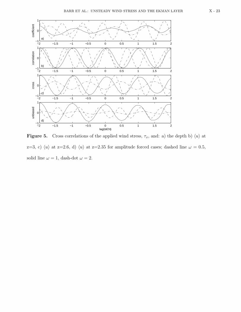
3.2.2. Correlations

Cross correlations between the wind stress and another variable give an indication as to

the time it takes for the Ekman layer to adjust to the forcing environment. The unbiased

cross correlation coefficients, the ratio of the cross covariance normalized by the standard

deviations, are calculated by:

C =2

∑

∆t=0

1

M

(τx(t) − τx)(〈B(zi, t + ∆t)〉 − 〈B〉)√

τx(t)2√

〈B(zi, t + ∆t)〉2(9)

where zi is at a fixed vertical location, B is either the horizontally averaged u-velocity or

the Ekman depth, and M is the number of samples in the signal.

The sub-resonant case shows strong correlation of e-folding depth with the amplitude

of the forcing. The depth lags the forcing by approximately one quarter inertial period.

The cross correlation between the forcing and 〈u〉 decreases with depth, yet all still have a

recognizable sinusoidal shape. Mid-layer, where the Ekman layer has flow in the opposite

direction to the wind stress, has the strongest negative correlation at a lag of -0.125.

With super-resonant forcing, the correlation of forcing and depth is lower than the sub-

resonant case. As seen in Figure 4, the depth of the Ekman layer is more constant in time

for ω = 2, leading to the lower correlation coefficient.

For resonant wind conditions, the depth is relatively weakly correlated with the applied

wind stress, as the layer steadily increases while the wind stress oscillates. The closest

peak to zero lag occurs at approximately 0.19, and a correlation coefficient of 0.25. This

implies that it takes roughly one fifth of an inertial period for the Ekman layer to adjust to

a resonant wind stress. The forcing, however, is strongly correlated with the horizontally

averaged u-velocity across the entire layer.


3.2.3. 1-D model results

Using the results from the full LES simulations, the values for the effective viscosity,

Az, can be calculated from equation (8). Instantaneous values are then phase averaged.

The results are seen in Figure 6. An additional step must be taken in the resonant case.

With each passing inertial period, the depth of the boundary layer increases in a step like,

self-similar manner. The thickness of the layer has to be normalized in order to complete

the phase averaging. This normalized vertical coordinate, ζ, is used in Figure 6b. For

all cases, there is an increase in the eddy viscosity at times of decreased forcing. This

corresponds with increased turbulent stresses, or decreased mean velocity gradients.

A comparison of the full LES model with the simplified 1-D effective viscosity model

can be made by comparing phase plane plots as in Figure 8 and Figure 7 for the case

ω = 2. Each frame contains parametric plots of 〈u(zi, t)〉 vs. 〈v(zi, t)〉 at different vertical

locations. The qualitative comparison between the two models is quite good, with each

showing a potential period doubling in the orbits of 〈u〉 and 〈v〉.

The double loop trajectory can be explained by comparing the applied forcing to the

inertial frequency. A schematic of this is shown in Figure 9. When the forcing and the

inertial frequency are in phase, the velocities increase, with 〈u〉 and 〈v〉 following the

larger loop. During the out of phase portion, the inner smaller loop is traversed.cl

3.3. Directional forcing

For directional forcing, the magnitude of the total wind stress remains constant, however

the magnitudes of each component (τx, τy) varies as the wind direction changes sinusoidally

from 45o to 180o. Evidence of periodic turbulent bursts can be seen in Figure 10. The

sub-resonant case is unstable with directional forcing; the horizontally averaged mean


kinetic and turbulent kinetic energy penetrate the domain roughly half as quickly as in

the resonant case. The super-resonant case remains stable.

3.3.1. Depth of the Ekman layer

The result of varying the wind direction on the Ekman layer depth can be seen in

Figure 11. The sub-resonant case, shows a resonant-like growth in the boundary layer

thickness, though at half the rate. A double lobe structure (smaller downward penetra-

tions of mean current at even numbered inertial periods, and larger excursions at odd

inertial periods )is evident in the current profile in Figure 10

In the case of resonant forcing, the layer again grows rapidly, at roughly the same rate

as the resonant amplitude forced case.

Notice that for super-resonant forcing, the layer can become nearly 4 times deeper than

the steady case. The super resonant case still suffers from “drop outs” in the measurement

of the depth due to the periodic disappearance of the mean current. In contrast to the

amplitude forced cases, the depths obtained from the mean current and the mean turbulent

kinetic energy are very similar, 1.1 and 1.3 respectively.

3.3.2. Correlations

The cross correlations of one component of the applied wind stress, τx, against the

measured layer depth and the horizontally averaged u-velocity at three different depths

are shown in Figure 12. For both sub-resonant and resonant forcing, the depth is only

weakly correlated with the forcing. In both cases, the layer grows relatively constantly,

regardless of what phase the forcing is in. With super-resonant forcing, the depth is more

strongly correlated with the forcing, showing a sinusoidal response. The depth lags the

forcing by approximately one tenth of an inertial period.


In the case of resonant forcing, the horizontally averaged u-velocity is strongly correlated

at all three depths investigated. For the off-resonant cases, the velocity at the surface

correlates strongly with the forcing, but that correlation decreases sharply with depth.

3.3.3. 1-D model results

In a similar fashion to the amplitude forced cases, the effective eddy viscosity can be

extracted from the full LES simulations for use in the simplified 1-D model. The results

are shown in Figure 13.

For wind direction forcing, the two cases that exhibit resonance are treated in a manner

similar to the resonant amplitude forced case. Notice that for the sub-resonant case that

there are two periods of relatively strong turbulence. The first burst occurs when the

forcing is in phase with the inertial current. That is followed by a period of weaker

turbulence as the inertial current goes directly out of phase with the forcing. The second

stronger burst occurs when the forcing is at a minimum, as is the inertial current.

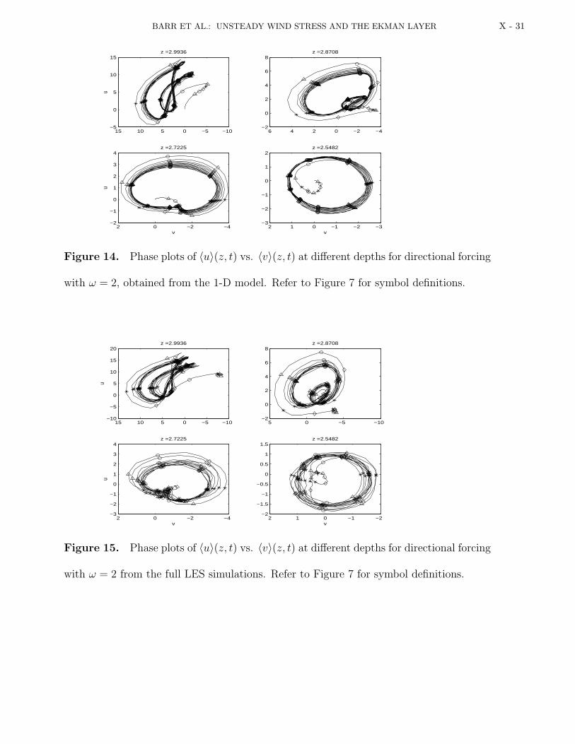
Using the effective eddy viscosity from Figure 13c, for ω = 2, the 1-D model results are

compared to the full LES model in Figure 14 and 15. A distinct double loop trajectory is

seen near the surface, with the larger loop being traversed when the inertial current and

forcing are in phase. The loops merge into a single trajectory which takes two inertial

periods to travel as the depth increases.


4. Conclusions

In this paper we have investigated the effect of an unsteady wind stress on the turbulent

Ekman layer. This study has shown that an unsteady wind stress can have a large impact

on the measured depth of the Ekman layer, increasing the depth of the layer by a factor

of four in some cases.

We found that the phase averaged effective viscosity varies significantly across the layer,

and that the simplified 1-D model agrees qualitatively with the full LES simulations. Since

the simpler model contains no information about either the latitude or direction of wind

stress, quantitative agreement cannot be expected, as shown in the case of steady wind

stress.

Turbulent bursts at times of minimum forcing, when the inertial current is weak are

responsible for the transport of turbulent energy deeper into the water column. With

resonant forcing, this penetration leads to finite values of turbulent kinetic energy near

the bottom boundary, leading to a numerical instability and the subsequent demise of

the simulation. A resonant effect was found to occur in a case of off-resonant forcing

(directional forcing with ω = 0.5).

The relative transience of the wind stress appears in the discrepancy of the Ekman layer

depth as measured by the mean current or the mean turbulent kinetic energy. This may

help observationalists that don’t have wind data.

Future improvements on the model includes allowing for density stratification and di-

urnal heating and cooling. With the improvements, it should become possible to model

results obtained from other in situ measurements.


References

Chereskin, T. K. & Roemmich, D., A comparison of measured and wind-derived Ekman

transport at 11oN in the Atlantic ocean, J. Phys. Ocean. 21, 869–878, 1991.

Craik, A. D. D. & Leibovich, S., A rational model for Langmuir circulation, J. Fluid

Mech. 73, 401–426, 1976.

Csanady, G. T., On the “resistance law” of a turbulent ekman layer, J of Atmos. Sci.24,

467–471, 1967.

Ekman, V. W., On the influence of the earth’s rotation on ocean currents. Arch. Math.

Astron. Phys. 2, 1–52, 1905.

Coleman, G. N., Ferziger, J. H. & Spalart, P. R., A numerical study of the turbulent

Ekman layer, J. Fluid Mech. 213, 313–348, 1990.

Lilly, D. K., A proposed modification of the Germano subgrid scale closure method, Phys.

Fluids A 4, 633–635, 1992.

Pope, S. B., Turbulent Flows, Cambridge University Press, 2000.

Price, J. F., Weller, R. A., & Schudlich, R. R., Wind-driven ocean currents and Ekman

transport. Science 238, 1534-1538, 1987.

Schudlich, R. R. & Price, J. F. Obseravtions of seasonal variation in the Ekman layer. J.

Phys. Ocean. 28, 1187–1204, 1998.

Skyllingstad, E. D., Smith, W. D., & Crawford, G. B., Resonant wind-driven mixing in

the Ocean boundary layer, J. Phys. Ocean. 30, 1866–1890, 2000.

Zikanov, O., Slinn, D.N., & Dhanak, M. R., Large-eddy simulations of the wind-induced

turbulent Ekman layer, accepted for publication in J. Fluid Mech.


Acknowledgments. This work was supported by the Office of Naval Research grant

N00014-00-1-0218 and NSF grant OCE-02-96010.


N

E

x

y

45o

180o

wind direction

Figure 1. Figure showing N-E axes and x-y axes, with wind direction change. The

z-axis is perpendicular out of the page.


−10 −5 0 5 102

2.2

2.4

2.6

2.8

3

horiz. ave. vel.

z

a)

<u> LES<v> LES<u> 1−D<v> 1−D

0 1 2 32

2.2

2.4

2.6

2.8

3

rms vel.

b)

<urms

><v

rms>

<wrms

>

0 2 4 6 8 102

2.2

2.4

2.6

2.8

3

c)

z

<S> LES<S> 1−D<TKE> LES

0 0.005 0.01 0.0152

2.2

2.4

2.6

2.8

3

Az

d)

Figure 2. Horizontally and time averaged a) mean velocity profiles, b) RMS of turbulent

velocities, c) turbulent kinetic energy, 〈TKE〉, and current, 〈S〉, - location of the e-

folding depth from LES current, - location of e-folding depth from 1-D current, ∗ -

location of e2-folding depth from 〈TKE〉, and d) effective viscosity, Az.


24

68

10

12

1.52

2.53

z

ω =

0.5

02

46

12

34

1.52

2.53

ω =

1

05

10

24

68

10

12

14

1.52

2.53

ω =

2

05

10

24

68

10

12

1.52

2.53

z

01

2

12

34

1.52

2.53

t/2

π

01

2

24

68

10

12

14

1.52

2.53

02

4

Figure 3. Horizontally averaged current, 〈S〉, and turbulent kinetic energy 〈TKE〉, for

the amplitude forced cases.


0 2 4 6 8 10 120

0.5

1a)

0 0.5 1 1.5 2 2.5 3 3.5 4

0.5

1

1.5

2

b)

D

0 2 4 6 8 10 12 140

0.5

1

1.5c)

t/2π

Figure 4. Depth of the Ekman layer for a) ω = 0.5, b) ω = 1, and c) ω = 2, · · ·

measured using mean current, — measured using horizontally averaged turbulent kinetic

energy.


−2 −1.5 −1 −0.5 0 0.5 1 1.5 2−1

0

1

coef

ficie

nt

a)

−2 −1.5 −1 −0.5 0 0.5 1 1.5 2−1

0

1

corr

elat

ion

b)

−2 −1.5 −1 −0.5 0 0.5 1 1.5 2−1

0

1

cros

s

c)

−2 −1.5 −1 −0.5 0 0.5 1 1.5 2−1

0

1

unbi

ased

lag(ω/2π)

d)

Figure 5. Cross correlations of the applied wind stress, τx, and: a) the depth b) 〈u〉 at

z=3, c) 〈u〉 at z=2.6, d) 〈u〉 at z=2.35 for amplitude forced cases; dashed line ω = 0.5,

solid line ω = 1, dash-dot ω = 2.


0

0.005

0.01

0.015

0.02

0.025

0.03

0 0.1 0.2 0.3 0.4 0.5 0.6 0.7 0.8 0.9 10

0.5

1

1.5

2

2.5

3

z

a)

0.05

0.1

0.15

0.2

0 0.1 0.2 0.3 0.4 0.5 0.6 0.7 0.8 0.9 10

0.2

0.4

0.6

0.8

1

ζ

b)

0

0.005

0.01

0.015

0.02

0.025

0.03

0 0.1 0.2 0.3 0.4 0.5 0.6 0.7 0.8 0.9 1

0.5

1

1.5

2

2.5

c)

z

0 0.1 0.2 0.3 0.4 0.5 0.6 0.7 0.8 0.9 10

0.2

0.4

0.6

0.8

1

τ x

t (ω/2π)

d)

Figure 6. Phase averaged eddy viscosity for amplitude forcing and: a) ω = 0.5, b)

ω = 1, and c) ω = 2. Panel d) shows the forcing during one period.


−8−6−4−20−4

−2

0

2

4

6

8

10z =2.9936

u

−6−4−202−3

−2

−1

0

1

2

3z =2.8708

−2−1012−2

−1.5

−1

−0.5

0

0.5

1z =2.7225

v

u

−1−0.500.511.5−1.5

−1

−0.5

0

0.5

1z =2.5482

v

Figure 7. Phase plots of 〈u〉 vs. 〈v〉 at different depths for ω = 2 obtained from the 1-D

model. Symbols denote: 4 - maximum τx, - minimum τx, - midpoint of decreasing

τx, and ∗ - midpoint of increasing τx from the 1-D model with ω = 2.

−10−8−6−4−20−5

0

5

10

15z =2.9936

u

−6−4−202−3

−2

−1

0

1

2

3z =2.8708

−2−1012−2

−1.5

−1

−0.5

0

0.5

1z =2.7225

v

u

−1−0.500.51−1

−0.5

0

0.5

1z =2.5482

v

Figure 8. Phase plots of 〈u〉(z, t) vs. 〈v〉(z, t) at different depths for ω = 2 from the

full LES simulations. Refer to Figure 7 for symbol definitions.


0 0.1 0.2 0.3 0.4 0.5 0.6 0.7 0.8 0.9 1-1

-0.8

-0.6

-0.4

-0.2

0

0.2

0.4

0.6

0.8

1

inertial freqforcing freq

in phase out of phase in phase

Figure 9. Sketch comparing inertial frequency and a forcing frequency of ω = 2.


24

61.52

2.53

z

ω =

0.5

05

10

12

31.52

2.53

ω =

1

05

10

24

68

10

12

1.52

2.53

ω =

2

05

10

24

61.52

2.53

z

01

23

12

31.52

2.53

t/2

π

01

23

24

68

10

12

1.52

2.53

02

4

Figure 10. Horizontally averaged current, 〈S〉, and turbulent kinetic energy 〈TKE〉,

for the directionally forced cases.


0 1 2 3 4 5 6 70

0.5

1

1.5

2

a)

0.5 1 1.5 2 2.5 3 3.50

0.5

1

1.5

2

b)

D

0 2 4 6 8 10 120

0.5

1

1.5

2

c)

t/2π

Figure 11. Influence of directional forcing on the Ekman layer depth, a) ω = 0.5, b)

ω = 1, and c) ω = 2, · · · measured using mean current, — measured using horizontally

averaged turbulent kinetic energy.


−2 −1.5 −1 −0.5 0 0.5 1 1.5 2−0.5

0

0.5

coef

ficie

nt

−2 −1.5 −1 −0.5 0 0.5 1 1.5 2−1

0

1

corr

elat

ion

−2 −1.5 −1 −0.5 0 0.5 1 1.5 2−1

0

1

cros

s

−2 −1.5 −1 −0.5 0 0.5 1 1.5 2−1

0

1

unbi

ased

lag(ω/2π)

Figure 12. Cross correlations of the applied wind stress, τx, and: a) the depth b) 〈u〉 at

z=3, c) 〈u〉 at z=2.6, d) 〈u〉 at z=2.35 for directionally forced cases; dashed line ω = 0.5,

solid line ω = 1, dash-dot ω = 2.


0

0.1

0.2

0 0.1 0.2 0.3 0.4 0.5 0.6 0.7 0.8 0.9 10

0.2

0.4

0.6

0.8

1

ζ

a)

0

0.05

0.1

0.15

0 0.1 0.2 0.3 0.4 0.5 0.6 0.7 0.8 0.9 10

0.2

0.4

0.6

0.8

1

ζ

b)

0

5

10

15

x 10−3

0 0.1 0.2 0.3 0.4 0.5 0.6 0.7 0.8 0.9 1

0.5

1

1.5

2

2.5

c)

z

0 0.1 0.2 0.3 0.4 0.5 0.6 0.7 0.8 0.9 1−1

−0.5

0

0.5

1

t (ω/2π)

τ

d)τx

τy

Figure 13. Phase averaged eddy viscosity for directional forcing and a) ω = 0.5,

b)ω = 1, c)ω = 2. Panel d) shows the wind stress components during one forcing period.


−10−5051015−5

0

5

10

15z =2.9936

u

−4−20246−2

0

2

4

6

8z =2.8708

−4−202−2

−1

0

1

2

3

4z =2.7225

v

u

−3−2−1012−3

−2

−1

0

1

2z =2.5482

v

Figure 14. Phase plots of 〈u〉(z, t) vs. 〈v〉(z, t) at different depths for directional forcing

with ω = 2, obtained from the 1-D model. Refer to Figure 7 for symbol definitions.

−10−5051015−10

−5

0

5

10

15

20z =2.9936

u

−10−505−2

0

2

4

6

8z =2.8708

−4−202−3

−2

−1

0

1

2

3

4z =2.7225

v

u

−2−1012−2

−1.5

−1

−0.5

0

0.5

1

1.5z =2.5482

v

Figure 15. Phase plots of 〈u〉(z, t) vs. 〈v〉(z, t) at different depths for directional forcing

with ω = 2 from the full LES simulations. Refer to Figure 7 for symbol definitions.

e ect of unsteady wind stress on the ekman layer

Documents