dynamique littorale et impacts socio-économiques en guyane...
TRANSCRIPT

Dynamique littorale et impacts socio-économiquesen Guyane française
Approche par télédétection spatiale
RAPPORT FINAL
JUIN 2004
ANTOINE GARDEL 1 ET NICOLAS GRATIOY
Institut de recherchepour 1 développement
V n;lr'~)! E(5'1.10)
Contrat de Consultance Institutionnelle IRD-CNES N° 02/CNES/0814/00
1 Unité ESPACE SJ40-IRD Guyanez Unité ELISA R053 -IRD Guyane

Dynamique littorale et impacts socio-économiques
SOMMAIRE
1 - INTRODUCTION 4A - CONTEXTE - PROBLEMATIQUE 5
B - CADRE DE L'ETIIDE 7
C - SYNOPSIS BIBLIOGRAPI-llQUE 81) Les côtes des Guyanes - Aspects de morphodynamique sédimentaire 82) Les origines de la dynamique et les répercussions géomorphologiques 83) Caractéristiques morphodynamiques des bancs de vase 104) Etudes par télédétection spatiale 11
2- MATERIELS ET M ETHODES 13A - LES SITES D'ETIIDE 13
1) Le littoral de Kourou 132) Le littoral de Mana 143) Le littoral de Sinnamary 154) Le littoral de Kaw 15
B - DE LA DONNEE BRUrE A L'INFORMATION TIIEMATIQUE 161) Données utilisées 162) Caractéristiques des données 173) Pré-traitements sur les données 17
C - EXTRACTION DES TIIEMES D'ETIIDE 22
1) Définition des thèmes d'étude 222) Extraction des thèmes sur les images. Système d'Information Géographique 22
D - METHODE POUR SUIVRE LA CINETIQUE DES BANCS DE VASE 231) Changement de repère 232) Correction des effets de marée 233) Représentation matricielle 25
3 - CINETIQUE D LITTORAL 27A - DYNAMIQUE DU LITTORALDE KOUROU 27
1) Cinétique du banc 272) Evolution des surfaces de mangrove 303) Interactions vase-végétation 31
B - RESULTATS SUR LES AUIRES BANCS 331) Commentaires généraux 332) Le rôle de l'orientation de la côte 343) Le rôle des estuaires 344) Des vitesses de déplacement homogènes 35
C - ROLE DES FORÇAGES EXTERNES 351) Génération des houles par le vent, généralités 352) Caractéristiques des vents locaux et globaux 363) Forçages et migration des banc 374) Perspectives de recherche sur l'action des houles dans la structuration côtière38
Contrat W02jCNESj0814jOO Page 2 Rapport final juin 2004

Dynamique littorale et impacts socio-économiques
~ - CARACTERISAnON DU BANC ET EVOLUTION DE L'EFFORT DE DRAGAGE39A - CARACTERISATION DE LAZONE INTER-TIDALE DU BANCPAR TELEDETECTION 39
1) Données utilisées 392) Méthode d'extraction 403) Réalisation d'un MNT 41
B - CARACTERISATION DE LA PARTIE SUB-TIDALE DU BANC 431) Matériels et méthodes 432) Traitements réalisés 44~~~~ %
C - HYPOTHESESDE FONCTIONNEMENT 48
5 - CONCLUSION
BIBLIOGRAPffiE
LISTE DES FIGURES
LISTE DES TABLES
ANNEXE 1
ANNEXE II
ANNEXE III
Contrat W02jCNESj0814jOO Page 3 Rapport final juin 2004
49
51
54
56
57
70
76
Dynamique littorale et impacts socio-économiques
1 - INTRODUCTION
Ce rapport présente les résultats de l'étude "Dynamique littorale et impacts socioéconomiques en Guyane française. Approche par télédétection spatiale" faisant l'objet d'uncontrat de consultance entre le CNES et l'IRD (N°02jCNESj0814jOO).
L'objet de cette consultance est de fournir au CNES, gestionnaire de l'accès au Port dePariacabo à Kourou, les outils nécessaires pour une meilleure gestion des actions de dragagequ'il a en charge.
Le travail réalisé comporte deux volets:1 : un volet scientifique visant à améliorer la compréhension des processus de dynamiquecôtière à la lumière des observations faite par satellite, en partenariat avec les équipes derecherche engagées sur le sujet à l'IRD et d'en d'autres organismes nationaux etinternationaux dans le cadre de programmes de recherches.
2 : un volet opérationnel visant :- à aider à une meilleure gestion du dragage par le suivi des mouvements d'envasementdésenvasement et de leurs effets sur l'estuaire.
Dans ce rapport, après avoir présenté le contexte et les enjeux induits, le cadre dans lequell'étude est réalisée est dressé.
Un synopsis bibliographique permet d'évaluer l'importance de la dynamique littorale surles côtes des Guyanes. Ce travail bibliographique souligne la grande variabilité de ladynamique de ces littoraux. Quelques travaux utilisant des données spatiales d'observationde la Terre pour suivre les modifications morphologiques de la côte ont montré la pertinencede ces techniques pour étudier un tel milieu.
Nous disposons aujourd'hui avec la filière SPOT, complétée de quelques donnéesLANDSAT, de suffisamment de recul (depuis 1986) pour étudier précisément lesmodifications morphologiques survenues sur le littoral guyanais et plus particulièrement surcelui situé entre Cayenne et Kourou (60km). L'exploitation de 59 images (acquises entre 1986et 2003) et l'utilisation d'un système d'information géographique, permettent de quantifierces modifications.
Une méthode est développée pour suivre et quantifier l'évolution spatio-temporelle del'installation puis de la migration du banc de vase qui se rapproche de Kourou. Les littorauxde Mana, Sinnamary et Kaw sont aussi étudiés sur la même période. Les trois-quart dulittoral guyanais de l'estuaire du fleuve Approuague à la frontière avec le Surinam sont ainsisuivis depuis presque 20 ans .
Les résultats obtenus permettent d'enregistrer de grandes variations spatio-temporelles de]a morphologie du littoral.
Les interactions entre la dynamique spatio-temporelle des bancs de vase et celle de lamangrove sont discutées. Elles mettent en évidence le rôle primordial des forçages externeset notamment de la houle comme principal agent de la dynamique côtière. Les forçages parIa houle sont étudiés en analysant des données de vent locaux et de vents synoptiques. Lesrésultats montrent le rôle principal des houles océaniques mais soulignent aussi les limitesliées aux données utilisées. L'utilisation de données issues de modèles de houle permettraitd'envisager des prévisions d'envasement ou d'érosion.
Contrat W02jCNFSj0814jOO Page 4 Rapport final juin 2004

Dynamique littoraleet impacts socio-économiques
Enfin, un dernier volet de ce travail a pour objectif de caractériser dans ses parties intertidale et sub-tidale le banc de Kourou et de proposer un scénario de fonctionnement prenanten compte l'évolution de l'effort de dragage dans le chenal d'accès au port de Pariacabo.
A CONTEXTE ET PROBLEMATIQUE
Les côtes de Guyane sont soumises à l'alternance de phases d'envasement et d'érosion. Lessédiments, provenant de l'embouchure de l'Amazone se déplacent sous la forme de bancs devase, en fonction de la saison et des conditions environnementales, le long des côtes del'Amapa et des Guyanes, jusqu'à l'Orénoque. De profondes modifications morphologiquesse font ressentir sur les côtes de la Guyane française et représentent de réelles contraintes auxactivités humaines.
En Guyane, 90 % de la population est localisée sur le littoral. La pression démographique estgrande (+ 37% entre 1990 et 1999 selon l'INSEE) et les enjeux de développement passent parde nombreux aménagements et par la construction d'infrastructures de communication.Face à la forte dynamique côtière les enjeux sont de taille et concernent toutes les activitéssocio-économiques. La région de Mana où l'érosion menace le littoral du village d'Awalamais aussi plus à l'est les aménagements rizicoles préoccupe aujourd'hui les décideurs. Lesplages de l'Ile de Cayenne et de Kourou, qui subissent périodiquement de fortes érosions(destructions d'habitations, d'infrastructures), suivies quelques années plus tard par unenvasement ont aussi pu faire l'objet d'inquiétudes. Les accès aux ports de Cayenne et deKourou doivent être périodiquement, voire constamment, dragués (pour le chenal duMahury). Ces actions de dragage sont primordiaux pour permettre aux navires (même defaible tirant d'eau) de débarquer. D'autres enjeux sont liés indirectement à la dynamiquecôtière. Ils sont d'ordre économique (la pêche notamment), d'ordre sanitaire (assainissement,épidémies de papillonite), d'ordre foncier et d'ordre touristique.
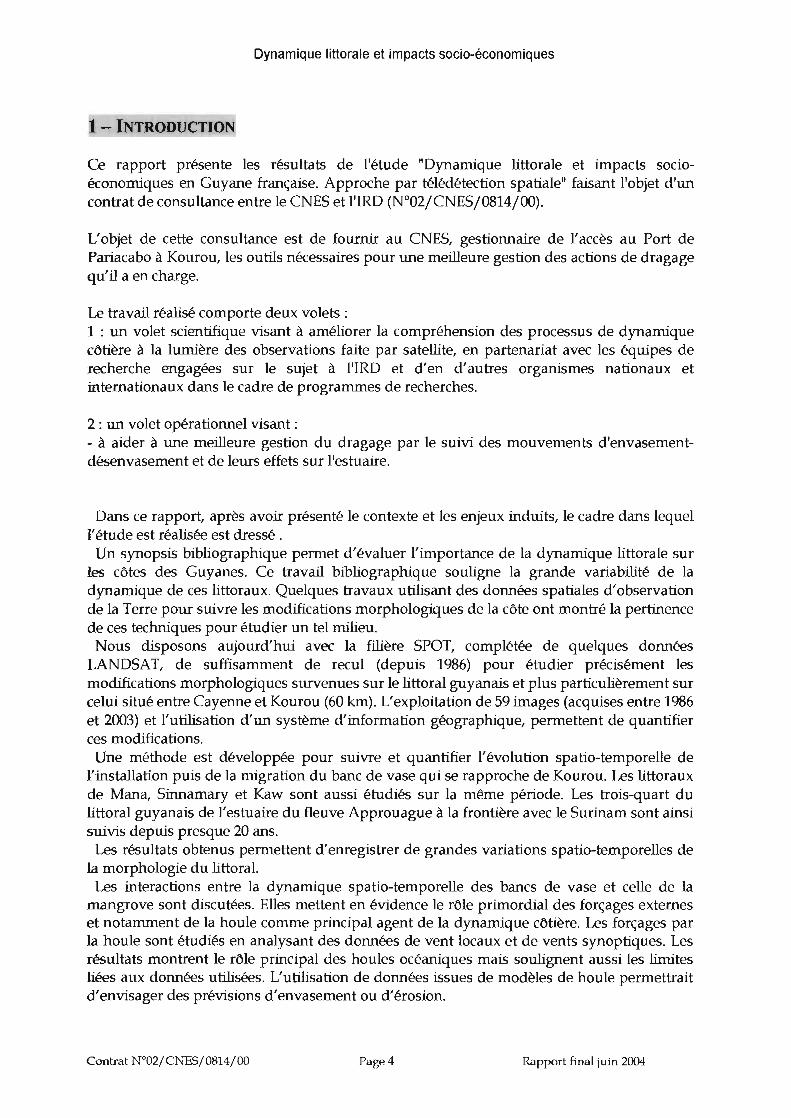
La Division des Infrastructures du Centre National d'Etudes Spatiales de Kourou par le biaisdu Bureau de Gestion Portuaire, a en charge l'entretien du chenal d'accès au Port dePariacabo. Un marché est passé avec la société de dragage "Atlantique Dragage", d'unmontant semestriel de l,OB million d'euros (premier semestre 2(03), pour assurer lanavigabilité dans le chenal et permettre aux navires d'accéder aux infrastructures portuairesde Kourou. Les navires Colibri et Toucan y débarquent en effet les éléments des fusées Ariane5 provenant d'Europe. C'est en 1994 que la mise au gabarit du chenal est réalisée. Entre 1994et 2ClC.XJ, seuls des dragages ponctuels (3 à 4 par an) sont effectués. Depuis 2ClC.XJ, le chenal estdragué en continu avec aujourd'hui un pompage effectif de 200 heures par mois. L'effort dedragage a évolué depuis 2ClC.XJ. Les premières actions de dragage se concentraient au niveaudu pk 8, c'est à dire au niveau de la sortie du fleuve Kourou en mer. En 2001, ils seconcentraient autour du pk 10 et en 2002 au pk 12. Aujourd'hui ils sont réalisés au delà dupk 13. Ces localisations sont présentées sur la figure 1.
On a aujourd'hui une bonne connaissance des causes géophysiques de l'instabilité du littoral.Les travaux menés depuis plusieurs décennies sur la morphodynamique du littoral guyanaisont permis de suivre l'évolution des bancs (partie émergée) et de mesurer leur vitesse dedéplacement par des approches théoriques et expérimentales. Toutefois, certains processusdynamiques restent encore mal connus concernant les facteurs de déplacement et deconsolidation des vases. La principale raison de cette lacune provient de la complexité dumilieu.
Contrat W02jCNFSj0814jOO PageS Rapport final juin 2004
Dynamique littorale et impacts socio-économiques
Figure 1 : le banc de vase se rapproche de Kourou. L'évolution de l'effort de dragage est représentéepar la localisation des pk et des années correspondantes. En fond, image SPOT (2001)
L'extension des zones concernées, les difficultés d'accès, la complexité des paysages et desmécanismes en jeux, font de l'observation de la Terre par satellite un outil incontournable enappui aux études physiques de terrain pour étudier les mécanismes de la dynamique côtière(déplacement des bancs, consolidation, colonisation par la mangrove) et les répercussionssur les activités socio-économiques. Avec 16 ans d'observations, la filière SPOT permetd'expertiser les phénomènes d'érosion et de sédimentation, et les performances inéditesd'ENVISAT et de SPOT-5, récemment lancés, offrent de nouvelles perspectives dansl'observation de la dynamique du littoral guyanais.
C'est dans un tel contexte que le CNES a contracté l'IRD pour réaliser l'étude: "Dynamiquelittorale et impacts socio-économiques en Guyane française. Approche par télédétectionspatiale". .Les objectifs principaux de ce travail sont de développer des outils utilisant la télédétectionspatiale pour étudier la dynamique du littoral de la région de Kourou. Les résultats de cetteétude permettront de mieux comprendre les mécanismes de la dynamique côtière et ainsid'aider à une meilleure gestion des actions de dragage.
Contrat W02jCNESj0814jOO Page 6 Rapport final juin 2004

Dynamique littorale et impacts socio-économiques
B CADRE DE L'ETUDE
Ce travail a été mené par l'Unité ESPACE S140 (Expertise et SPAtialisation desConnaissances en Environnement) de l'Institut de Recherche pour le Développement enGuyane en étroite collaboration avec l'Unité de Recherche ELISA (Ecosystemes littoraux sousinfluence amazonienne).
La spécialisation de l'IRD dans l'environnement tropical, et la diversité de ses travaux derecherche pour le développement lui confèrent un positionnement original au sein dudispositif de recherche national et international. Dans le cadre de programmespluridisciplinaires, des équipes de l'IRD et des organismes du Sud, exploitent depuislongtemps des données spatialisées et mettent en œuvre des approches multi-échellespermettant de mieux comprendre les phénomènes environnementaux et sociaux qui sedérobent aux analyses conventionnelles. Elles ont notamment acquis un savoir-faire reconnudans le domaine de l'observation de la Terre, des systèmes d'information environnementauxen milieux tropicaux et dans la mise en œuvre d'approches intégrées des milieux et dessociétés.
L'unité ESPACE, mobilise une cinquantaine de scientifiques et techniciens de l'IRD etd'autres organismes pour s'impliquer particulièrement dans deux champsd'activités complémentaires:
» les activités de recherche organisées autour de deux axes (observation de la Terre etapproches intégrées des milieux et des sociétés) pour approfondir et développer desméthodes d'analyse spatiale dans un souci d' opérationalité ;
» les activités de service pour répondre aux questions de développement en milieu tropicalnotamment au travers d'appui aux équipes internes IRD, de formation, d'expertise et devalorisation.
Le Laboratoire Régional de Télédétection (LRT), créé en 1994 en Guyane dans le cadre duXième Contrat de Plan Etat Région pour mettre en place un pôle de compétence entélédétection, a été intégré en 2002à l'unité ESPACE de l'IRD. Le LRTa développé au traversdu programme de recherche XIième CPER-FEDER des partenariats étroits avec des équipesde recherches travaillant sur la dynamique des côtes influencées par l'Amazone. Ces équipesnationales (autres Unités de 1'1RD, autres Instituts de recherche où Universités) etinternationales (essentiellement au Nord du Brésil: Macapa, Belèm, Sâo Luis) sont fédéréesdans le cadre du réseau de recherche ECOLAB qui a pour objectif l'étude des littoraux sousinfluence de l'Amazone.
L'Unité ESPACE coordonne le projet AGIL (Aide à la Gestion Intégrée des Littoraux) quiregroupe le ClRAD, IFREMER, BRGM, CNES, SCOT et BRU pour structurer au plannational et dans le cadre du Réseau Technologique Terre et Espace (Ministère de laRecherche) une offre de service pour la gestion intégrée des littoraux Les projets pilotesimpliquant les gestionnaires et utilisateurs concernent les zones côtières du LanguedocRoussillon, de la Réunion. Des chantiers de mise au point méthodologique ont été mis enplace en Guyane et en Nouvelle-Calédonie.
L'Unité est aussi impliquée dans le projet d'installation d'une station de réceptionSPOTIMAGE en bande X à Cayenne. Celle-ci, permettra d'acquérir à en Guyane les imagesdes différents satellites SPOT ainsi que les images ENVISAT. Ces données seront tout à fait
Contrat W02/CNFS/0814/00 Page 7 Rapport final juin 2004

Dynamique littorale et impacts socio-économiques
appropriées au suivi des littoraux de la région, ce que nous allons démontrer dans de ceprésent rapport.
C SYNOPSIS BIBLIOGRAPHIQUE
1) Les côtes des Guyanes - Aspects de morphodynamique sédimentaireLes côtes des Guyanes (Augustinus, 1990; Prost, 1990) comme celles de la Floride de l'ouest(Priee, 1955), du nord-est australien (Davies, 1980) et de certaines parties d'Afrique de l'ouest(Anthony, 1990) font partie des rares vraies côtes à cheniers au monde. Ces dernières sontdes côtes vaseuses, progradantes, généralement de basse énergie qui peuvent connaître desépisodes de processus hydrodynamiques de forte énergie contrôlés par la houle (Anthony,1990). Des cordons sableux appelés cheniers sont alors construits à partir de matériel grossier(sables, coquillages). Lorsque le régime hydrodynamique redevient normal, ils sont isoléspar un nouveau processus de progradation vaseuse (voir figure 2)
I{ v,~,~~ j-: ]+:~ .~;;cs Cheniers e e
+ -
Figure 2 : Passage des vasières aux cheniers marqué par une dominance croissante des processus dusaux vagues (d'après Anthony, 1990).
L'origine des sables qui composent les cheniers est locale (Pujos et al, 1990 et 2001).Cependant l'apport actuel des fleuves guyanais en sable ne semble pas suffisant (Fritsch,1984, Lointier et Prost, 1988a) pour maintenir les accumulations sableuses à la côte et formerde nouveaux cheniers de grande ampleur. Aujourd'hui, le développement de cheniers sur lelittoral de la Guyane est quasiment nul Les côtes sableuses visibles actuellement sont pour laplupart d'anciens cordons (Holocène) en érosion sous l'action de la houle. Toutefois, danscertains cas, des cheniers sont en place (exemple de la Pointe Macouria, à l'estuaire du fleuveSinnamary, dans l'ouest guyanais). De taille réduite (cordons minces), ils se forment à partirdu remaniement de petites quantités de sables enfermées dans les bancs ou apportéesdirectement aujourd'hui par les cours d'eau. Seules les sables anciens répartis sur le plateaucontinental sont fossilisés (Pujos et al, 1985) - d'où l'absence d'une progradation sableuse àgrande échelle.
Sans apport de sable massif, la dynamique sédimentaire du littoral de la Guyane estessentiellement vaseuse.
2) Les origines de la dynamique et les répercussions geomorphologiquesLes côtes des Guyanes, de l'état d'Amapa au nord du Brésil jusqu'au delta de l'Orénoque auVenezuela sont les côtes vaseuses les plus étendues au monde (Allison et al.,2(00). Elles sontconsidérées par certains auteurs comme étant un delta atténué de l'Amazone (Rine etGinsburg, 1985).La dynamique côtière de cette région située au nord-est de l'Amérique du sud est largementdominée par les interactions entre les houles, les courants côtiers et les sédiments provenantde l'embouchure de l'Amazone (Figure 2). La fréquence et l'intensité des apports
Contrat W02jCNESj0814jOO Page 8 Rapport final juin 2004

Dynamique littorale et impacts socio-économiques
sédimentaires sont variables, fortes en saison des pluies (janvier-juin) avec un maximum enavril-mai et plus faible en saison sèche (juillet-décembre) avec un minimum en aoûtseptembre (NEDECO, 1968; Allersma, 1971; Rine et Ginsburg, 1985).
Figure 3: La dynamique sédimentaire de l'Amazone à l'Orénoque. [mage multi-capteurs : sur l'océansynthèse multi-dates d'indice de turbidité sur 3 images NOAA (acquises au LRT), octobre 1999.Sur lecontinent la mosaïque d'images radar J-ERS acquises en 1995 permet d'obtenir des informations surles formations constituant le plateau des Guyanes .
La décharge sédimentaire de l'Amazone a été estimée à 1,2 milliard de tonnes/an (Meade etal., 1985). Quarante pour cent de ces sédiments (soit 480 millions de tonnes) migrent vers lenord ouest, le long des côtes des Guyanes dont la moitié en suspension dans les eauxcôtières, et l'autre moitié sous la forme de vastes bancs de vase accolés à la côte (Wells etColeman, 1981). Ces bancs de vase se forment le long de la côte nord ouest de l'Etat d'Amapaau Brésil (Allison et al., 20(0). Ils migrent ensuite le long des côtes de la Guyane française, duSurinam, du Guyana jusqu'au delta de l'Orénoque au Venezuela (Warne et al., 2002). Depuisl'Holocène, ce système de dispersion des vases de l'Amazone influe sur la morphologie descôtes de la Guyane française : l'envasement du littoral et la prépondérance des apportsd'origine amazonienne correspondent en effet à la remontée flandrienne de l'Holocèneinférieur (Prost, 1986). L'environnement côtier de la Guyane a fait l'objet de nombreuxtravaux. Prost (1990) a caractérisé les paysages côtiers anciens en distinguant deux grandesunités: une jeune plaine côtière datant de l'Holocène, qui se situe juste derrière la côtevaseuse contemporaine, et, plus en retrait, une plaine côtière ancienne d'origine Pléistocène.La première est caractérisée par la présence de marais herbacés et de forêts marécageuses. Laseconde se compose de savanes plus ou moins humides et s'étend sur 10 à 20 km dans lesterres jusqu'aux contreforts du Bouclier Guyanais. La plaine côtière humide est découpée par
Contrat N°02/CNES/0814/00 Page 9 Rapport final juin 2004

Dynamique littorale et impacts socio-économiques
d'anciennes lignes de rivages sableuses Holocènes (anciens cheniers). Le littoral évoluerapidement. 11 peut être vaseux ou sableux en fonction de la présence d'un banc de vase etd'une érosion intense qui attaque d'anciennes lignes de rivage. Les phases d'envasement sontcaractérisées par l'installation de vastes bancs de vase qui une fois stabilisés sont coloniséspar une mangrove pionnière. La phase d'inter-bancs se caractérise quant à elle par uneérosion intense qui a pour effet de re-mobiliser les sables Holocènes et de former deslittoraux sableux (cheniers ou cordon sableux), comme décrit auparavant.
3) Caractéristiques morphodynamiques des bancs de vaseLes caractéristiques morphologiques des bancs de vase ne sont pas bien connues. Leurmorphologie apparaît comme étant très variable. Les dimensions des bancs varient: de 10 à60 km de longueur, de 20 à 30 km de largeur et d'environ 5 mètres d'épaisseur, les espacesinter-banc sont espacés de 15 à 25 km (Froidefond et aL, 1988; Allison et al., 2(00). En l'étatactuel des connaissances, ils peuvent être schématisés comme présenté dans la figure 4.
Figure 4: Schématisation d'un banc (d'après Baghdadi el al. 2004). La partie immergée en permanence(zone sub-tidale) n'est pas précisément délimitée. L'avant du banc est constitué de vases fluides (quiconstituent des lacs de vase). La zone inter-tidale, zone de balancement des marées est colonisée danssa partie arrière par de la mangrove. De part el d'autre du banc les espaces inter-bancs sont en érosion.
Les taux de migration des bancs de vase sont aussi très variables, de moins de 0,5 km par anà plus de 5 km par an (Augustinus, 1987; Eisma et al., 1991; Froidefond et al., 1985 et 1988).Cette migration a pour principal moteur la houle générée par les vents dominants quiatteignent un maximum d'intensité entre décembre et mars (Wells et Coleman, 1981). Desrécents travaux menés par Rodriguez et Mehta (1998) ont montré que le courant desGuyanes, considéré jusqu'alors comme un des principaux agents de la migration des bancs,était bien trop au large pour avoir un réel effet sur le transport des vases côtières.Augustinus (1987) a aussi montré l'importance de l'orientation de la côte par rapport àl'angle d'incidence des houles dans les variations des taux de migration. Le tableau 1présente les caractéristiques des bancs sur les côtes des trois Guyanes.
Contrat W02jCNESj0814jOO Page la Rapport final juin 2004

Dynamique littorale et impacts socio-économiques
Dates des Vitesse Angle incidencephotos Km/an de la houle (NE)
19421950 10°
Guyana1962/1964 0.5-2.5 "<1972/19751979/198019841947/19481957 45°
Surinam 1966 0.5- 5.5 --L197019811955
Guyane française1979 0.3-1.4 3~1982 15°1984
10-60 km de long3-5 km de large
Paramètres morphologiques des 5 m épaisseurbancs de vase (partie inter-tidale) interbanc 8-26 km de long
pentes :entre 1:3000 et 1:500 (du banc)Marée (m): 0.6-3.6
Paramètres physiques communsHoule: E NEhauteur (m) 0.5-1.5période (s) 6-12
Tableau 1 : Caractéristiques des bancs observées sur photographies aériennes et particularitésenvironnementales communes aux trois pays.
Les taux de migration présentés auparavant sont le résultat de travaux utilisant desphotographies aériennes. Compte tenu des contraintes d'acquisition et de traitement desphotographies aériennes (contraintes climatiques, coüts élevés), l'utilisation de ces donnéesest rendue difficile pour un suivi régulier.A notre connaissance, depuis le travail de NEDECO (1968) aucun suivi de la migration desbancs à l'échelle régionale, c'est à dire de leur formation au Brésil jusqu'à leur disparition auVenezuela nia été entrepris. Un tel travail permettrait de comparer simultanément, enutilisant des méthodes identiques, les taux de migration des bancs pour aider à lacompréhension des variations.
4) Etudes par télédétection spatialeLes études sur la dynamique côtière de cette région utilisant la télédétection spatiale sontréalisées essentiellement en Guyane française. Elles ont fait l'objet, soit d'études de projetspilotes de l'ESA, soit de rapports issus de contrats de consultance, soit de travaux derecherche réalisés dans le cadre de programmes nationaux (Programme Nationald'Environnement Côtier)
Contrat W021CNFS/0814100 Page 11 Rapport final juin 2004

Dynamique littorale et impacts socio-économiques
a) Etudes Projets-pilotesDes études prospectives utilisant des données radar, dans le cadre de projets pilotes de l'ESAsont menées dans les années 1990 (Rudant et al. 1993, 1995). Elles montrent l'intérêt de tellesimages dans le contexte amazonien. Toutefois elles n'ont été que peu utilisées depuis.
b) Rapports (conventions et stages d'étudiants)La plupart des travaux réalisés ont fait l'objet de convention entre l'ORSTOM et le ConseilRégional de la Guyane (Lointier et Prost, 1988b) et entre l'ORSTOM et EDF (LRT, 1997).Cestravaux ont montré les potentialités des images de télédétection spatiale pour suivre lesévolutions morphologiques du littoral. De la même façon des rapports de stage dont celui deLebourgeois (2002) ont étudié ponctuellement l'évolution d'une partie du littoral.
c) Travaux issus de programmes de rechercheDans le cadre du Programme National d'Environnement Côtier des travaux utilisant latélédétection spatiale se sont intéressés à la turbidité des eaux côtières (Froidefond et al. 2000et 2(01). Des travaux utilisant des images radars pour étudier la dynamique des bancs devase sont en cours de réalisation dans le PNEC par les équipes du BRGM d'Orléans(Baghdadi et al., 2004).
Toutefois la dynamique des bancs de vase à proprement parlé n'a été que peu étudiée partélédétection spatiale et surtout n'a jamais été étudié avec plus de 15 années de recul.Les travaux les plus significatifs qui ont quantifié cette dynamique sont ceux citésauparavant utilisant des photographies aériennes.
Contrat W02jCNESj0814jOO Page 12 Rapport final juin 2004
Dynamique littorale et impacts socio-économiques
2 - MATERIELS ET METHODES POUR SUIVRE L'EVOLUTION DU LITTORAL
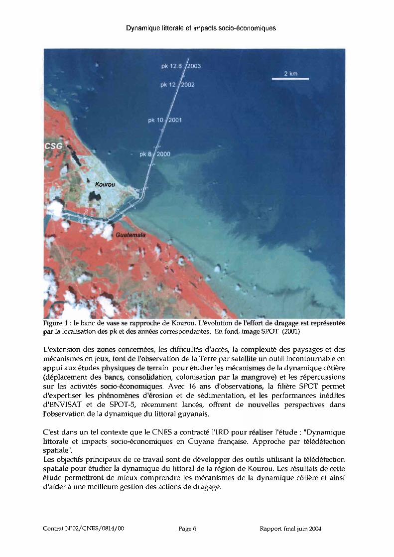
Dans le rapport intermédiaire, nous présentions la méthode développée et utilisée pourquantifier la dynamique côtière sur le littoral de Kourou (Gardel et Cratiot, 2(03). Cetteméthode est rappelée dans le présent rapport. Plusieurs sites en plus de Kourou sont étudiésdans l'objectif de comprendre le rôle des particularités géomorphologiques locales dans ladynamique littorale. La méthode est appliquée à trois autres sites du littoral guyanais: lelittoral de Mana, celui de Sinnamary et celui de Kaw. Les caractéristiques physiques des sitesseront présentées dans ce chapitre.Au total, 59 images couvrant une grande partie du littoral guyanais sont utilisées dans cetteétude. Un tel nombre donne un aperçu des possibilités que la station de réception d'imagesSPOT qui devrait être installée en Guyane offrira en terme de surveillance du domaine côtier.
A - LES SITES n'ETUDE
Les principales caractéristiques géographiques de chacun des sites sont présentées brièvement ici.
Mana
Sinnamary
Kourou
Kaw
Figure 5 : Le littoral guyanais del'Approuague à l'est au Maroni à l'ouest.MOSaïque de 4 images satellites (1986région de Sinnamary et Kourou, 1987région de Mana et 1988 région de Kaw)
1) Le littoral de KourouDepuis la rivière de Cayenne, délimitant l'Ile de Cayenne dans sa partie occidentale jusqu'aulittoral du CSG, la côte est quasiment linéaire, avec une orientation relativement homogène,de l'ordre de 15° (voir Figure 6). Les deux principaux cours d'eau (le fleuve Kourou et larivière de Cayenne) ont une sortie directe en mer (c'est à dire que ces estuaires ne présententpas de déviation vers le nord-ouest comme l'ont la plupart des estuaires guyanais). Ceci estdu aux affleurements du socle de la pointe des Roches et de l'Ile de Cayenne, qui stabilisentces deux embouchures. Par ailleurs, de nombreux hauts fonds rocheux sont présents de part
Contrat W02/CNES/0814/00 Page 13 Rapport final juin 2004

Dynamique littorale et impacts socio-économiques
et d'autre de l'estuaire du fleuve Kourou. Ces affleurements ne sont pour la plupart pasrépertoriés sur les cartes marines; certains d'entre eux ont pu être localisés à partir desimages satellites; ils sont reportés sur la Figure 28.
Figure 6 : Le littoral dans larégion de Kourou. Les troisthèmes extraits des imagessont représentés (gris :vase, mauve: mangrove,moutarde: trait de côte).
1iI ~-"":-...H':- .-"' ...-.."..~ ..--.~\ ....,~,,,-~, ...~ III....3 ••H--.-:' :.-; ..::,t".-..~ ..., ,, ....".-'-.
2) Le littoral de ManaLe site de Mana dans l'ouest subit une érosion intense depuis plusieurs décennies.L'orientation de la côte dans cette région diffère du reste de la Guyane (350 contre 150
ailleurs) et annonce l'orientation est-ouest de la cOte surinamaise. L'analyse des imagessatellites ne révèle pas la présence de hauts fonds rocheux dans la région. Il est à noter quel'estuaire de la Mana, d'orientation sud-est nord-ouest, est en profonde modification depuisune dizaine d'années (érosion de la Pointe Isère et ouverture d'une brèche) . Aujourd'hui, lesrizières sont menacées (déjà 500 hectares sont abandonnés à la mer) ainsi que le village deAwala-Yalimapo (école emportée, cimetière et stade de football menacés).Nous disposons sur ce site de 10 images satellites (3 landsat TM et 7 SPOT dont 3 achetéesgrâce à un bon ISIS).
Figure 7 : Le littoral dans larégion de Mana. Les troisthèmes extrait des imagessont représentés (gris :vase, mau ve : mangrove,moutarde: trait de côte). Anoter que les rizières etmarais sub-côtiers sontintégrés dans le thèmemangrove.
Contrat N°02/CNES/0814/00 Page 14 Rapport final juin 2004
. ~
~ ~ tt ..
~ :: ~ .: tt..:: ~
:>~:> ~-
~ ~
. ~ :> ~:- ~ ..,, ~ .='t't...~ ~ ..
~ ::: ~ ..- ~ -- ~ -., ~-
.~ -
~ ~ ~~
~ ~
- ~ ::_....
= ~ .- 1

Dynamique littorale et impacts socio-économiques
3) Le littoral de SinnamaryEn termes de dynamique sédimentaire et de dynamique de la mangrove, le site deSinnamary est, tout à fait original. Effectivement, c'est au niveau de l'estuaire du fleuveIracoubo que l'orientation de la côte guyanaise change. On trouve dans la région les bancs devases les plus étendus mais aussi les forêts de mangrove les plus importantes (estuairecommun de la Counamama et de l'Iracoubo) de Guyane. Les estuaires ont une orientationsud-est nord-ouest. Tout comme celui de Mana, l'estuaire du fleuve Sinnamary a connul'ouverture d'une brèche. Actuellement la mangrove d'Iracoubo subit une érosionimportante. Le littoral au sud-est de Sinnamary est jonché de hauts fonds rocheux dont les« battures de la Malmanoury » .
Figure 8 : Le littoral dans larégion de Sinnamary. Deuximportants estuaires sontprésents dans cette région :Iracoubo-Counamama etSinnamary.
4) Le littoral de KawLe littoral de la région de Kaw, au sud-est de l'Ile de Cayenne, se situe entre deux estuairesmajeurs, à savoir l'Approuague et le Mahury. Tout deux présentent une sortie directeorientée « sud-nord »., Situé à mi-distance du littoral, l'estuaire de la rivière de Kaw est demoindre importance avec des débits de quelques dizaines de m3/s. Il présente uneorientation sud-est nord-ouest, comme la plupart des embouchures guyanaises (Mana,Sinnamary, Iracoubo). Sur ce site aussi, une brèche a été ouverte il y a une dizaine d'annéespar l'érosion. Les mangroves de Kaw sont elles aussi étendues et anciennes (en arrièremangrove).
Figure 9 : Le littoral dans larégion de Kaw.
Contrat W02/CNFS/0814/00 Page 15 Rapport final juin 2004
. j~ l:t - .
~ ~
- \ .~ ~ ..., ~ ~
- ~ ~. ~~
. ~~,,\
. \ ~
.::lt~ " ...,, ~
-'" ~ -- ~ ~,, ~-
" '~,, ~ --'" ~ ~:! f:!I ...-, ~
- ~ ~,, ~~
- .~-,-~ ~ ..." ~...: ~-

Dynamique littoraleet impacts socio-économiques
B - DE LA DONNEE BRUTE A L'INFORMATION THEMATIQUE
1) Données utiliséesSur la période 1986 à 2003, nous avons pu disposer de 17 images SPOT et d'une imageLANDSAT pour couvrir (voir Tableau 2 et Figure 5) le site de Kourou. Au total, 18 imagesdont quatre LANDSAT ont été utilisées pour le site de Sinnamary, 10 images dont quatreLANDSAT pour le site de Mana et 8 images dont 1 LANDSAT pour le site de Kaw.Cinq images acquises sur le site de Kourou à un mois d'intervalle et à des hauteurs de maréedifférentes ne sont pas utilisées dans ce volet et seront présentées dans le dernier chapitre.
n° imaae Région images date heure niv. Marée***
1 Kourou SPOT 20-oct-86 11h16 1,282 Kourou SPOT 17-nov-91 11h13 2,4
3 Kourou SPOT 02-oct-93 10h56 1,144 Kourou SPOT 30-août-94 11h12 2,28
5 Kourou SPOT 16-oct-95 10h49 2,356 Kourou SPOT 26-oct-95 10h57 1,147 Kourou SPOT 28-sept-96 10h55 0,86
8 Kourou SPOT 02-sept-97 11h20 0,979 Kourou SPOT 20-juin-98 10h57 2,11
10 Kourou SPOT 06-sept-98 10h57 0,7411 Kourou SPOT 09-mai-99 10h45 2,6512 Kourou SPOT 07-févr-00 11h16 1,213 Kourou SPOT 02-juil-01 10h49 1,5814 Kourou SPOT 14-oct-01 10h49 1,4
15 Kourou SPOT 14-déc-01 11h16 1,2816 Kourou SPOT 05-aout-02 11h15 1,78
17 Kourou Landsat 19-sept-02 10h00 1,0518* Kourou SPOT 13-août-03 11h18 0,87
19 Sinnamary SPOT 20-oct-86 11h17 1,28
20 Sinnamary Landsat 23-iuil-87 10h00 1,6121 Sinnamary SPOT 27-oct-89 11h05 1,53
22 Sinnamary SPOT 06-sept-91 10h58 1,23
23 Sinnamary SPOT 17-juin-92 11h17 1,67
24 Sinnamary Landsat 22-sept-92 10h00 2,23
25 Sinnamary SPOT 28-oct-93 10h56 1,51
26 Sinnamary SPOT 03-août-95 11h12 2,3527 Sinnamary SPOT 28-sept-96 10h55 0,86
28 Sinnamary Landsat 03-août-97 10h00 1,67
29 Sinnamary SPOT 02-sept-97 11h20 0,97
30 Sinnamary Landsat 21-nov-99 10h00 1,44
31 Sinnamary SPOT 08-févr-00 10h57 1,45
32 Sinnamary SPOT 23-nov-01 11h19 2,47
33 Sinnamary SPOT 14-déc-01 11h16 1,2834* Sinnamary SPOT 26-juil-02 11h07 1,7335 Sinnamary SPOT 01-oct-02 11h19 2,2936 Sinnamary SPOT 07-oct-02 11h04 0,7537 Mana Landsat 23-iuil-87 10h00 1,6138 Mana SPOT 17-iuin-92 11h17 1,67
39 Mana Landsat 22-sept-92 10h00 2,2340 Mana Landsat 03-août-97 10h00 1,6741* Mana SPOT 10-août-98 11h17 1,52
Contrat N°02/CNFS/0814/00 Page 16 Rapport final juin 2004

Dynamique littorale et impacts socio-économiques
42 Mana Landsat 21-nov-99 10h00 1,44
43 Mana SPOT 28-juil-00 11h09 2,0444 Mana SPOT 23-sept-01 10h53 3,0645* Mana SPOT 26-juil-02 11h07 1,7346* Mana SPOT 26-août-03 10h53 1,3847 Kaw Landsat 18-iuil-88 10h00 2,48
48** Kaw SPOT 17-nov-91 11h13 2,4849** Kaw SPOT 20-juin-98 10h57 2,0250** Kaw SPOT 15-août-99 11h00 2,0551** Kaw SPOT 05-dec 00 11h00 2,6452 Kaw SPOT 14-déc-01 11h16 1,16
53** Kaw SPOT 05-aout-02 11h15 1,7654** Kaw SPOT 13/0812003 11h18 1,19
Tableau 2 : liste des images utilisées dans l'étude sur la cinétique côtière. * images acquises grâce à unbon ISIS, ** images acquises dans le cadre du chantier PNEC-Guyane grâce à des bons ISIS. ***prévision du SHOM.
2) Caractéristiques des donnéesLes capteurs optiques à haute résolution tel que SPOT et LANDSAT acquièrent des imagesdans les longueurs d'ondes du visible et de l'infra-rouge (bande xs1: 500-590 nm; bande xs2:610-680 nm; bande xs3: 7SD-S9Onm; bande xs4: 15SD-175Onm pour SPOT en mode multispectral). Les résolutions spatiales des données utilisées (de 2.5 à 20 mètres pour SPOT et 30mètres pour LANDSAT) sont suffisantes pour étudier le littoral. Les contraintes climatiquesen Guyane peuvent limiter l'utilisation des images optiques. Toutefois, à l'heure de passagede SPOT (14h00 TU) et de LANDSAT (13h00 TU), le frange côtière est souvent dégagée denuages du fait des alizés.
3) Pré-traitements sur les donnéesToutes les images sont corrigées géométriquement, informées dans un même référentielcartographique (WGS84) et sont projetées en UTM Nord Zone 22. Ces pré-traitements sontréalisés sous le logiciel de traitement d'images ER Mapper (©) software version 6.21. Lesimages géoréférencées sont ensuite intégrées dans un système d'information géographique(GeoConcept ©).
Contrat W02/CNES/0814/00 Page 17 Rapport final juin 2004

Dynamique littorale et impacts socio-économiques
Contrat N °02jCNESj0814jOO Page 18 Rapport final juin 2004

Dynamique littorale et impacts socle- économiques
-,.:,..
' .
Contrat N°02jCNESj0814jOO
25
Page 19
-Iracoubo20
Rapport final juin 2004
21
24
27

Dynamique littorale et impacts socio-économiques
Région de Mana
Contrat W02jCNESj0814jOO
37
43
45
Page 20 Rapport final juin 2004
38
44
Dynamique littorale et impacts socio-économiques
Région de Kaw
48
49 50
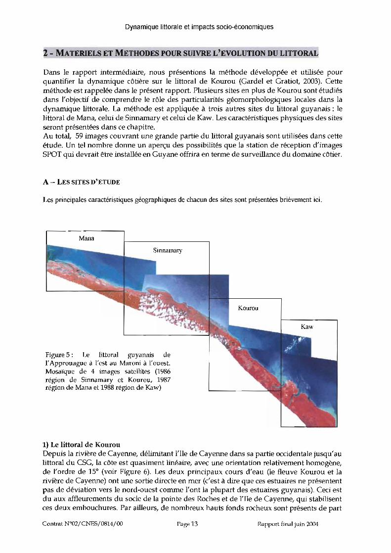
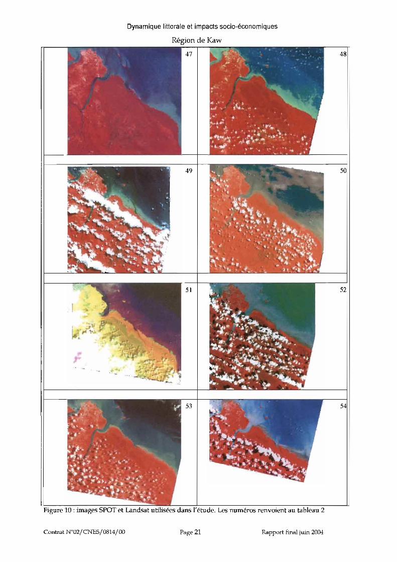
Figure 10: images SPOT et Landsat utilisées dans l'étude. Les numéros renvoient au tableau 2
52
54
Contrat N °02jCNFSj0814jOO Page 21 Rapport final juin 2004

Dynamique littorale et impacts socio-économiques
C - EXTRACTION DES THEMES D'ETUDE
1) Définition des thèmes d'étude.Deux thèmes ont été identifiés pour suivre la cinétique du littoral à différentes dates: lamangrove et la vase inter-tidale. L'objet "trait de côte stable" est aussi considéré pour l'étude.fis sont représentés dans la figure suivante
La définition d'un "trait de côte stable", qui servira de référence pour suivre l'évolutionlittorale, n'est pas évidente en Guyane compte tenu des profondes modificationsmorphologiques du littoral. Nous avons choisi de prendre le premier cordon holocène setrouvant en arrière de la mangrove. Nous verrons par la suite que ce trait de côte subitdepuis peu une érosion importante dans la région nord ouest du site de Kourou.Le thème "mangrove" correspond à la végétation se trouvant entre le cordon et l'océan.Cette végétation se développe dans la zone inter-tidale du banc de vase. Lespeuplements forestiers qui constituent la mangrove sont souvent homogènes et sontdonc facilement identifiables puisqu'elles présentent des signatures de réflectancemarquées.Le thème "vase" correspond à la partie inter-tidale du banc étant exondée lors de la prised'image. Sur les images de télédétection il n'est pas possible de délimiter les bancs devase dans leur partie sub-tidale. Seules des campagnes de bathymétrie couplées à destraits de bennes (pour déterminer la concentration de la vase) permettent de délimiter lebanc au large (Gratiot et al. 2(03). La partie inter-tidale, c'est à dire émergée à maréebasse, est donc la seule partie du banc qui peut être suivie sur les données detélédétection (images et photos).
2) Extraction des thèmes sur les images. Système d'Information GéographiqueLes thèmes d'étude sont extraits selon une méthode manuelle qui consiste à interpréter lesimages et à numériser les limites des objets. Ce travail est réalisé à chaque date. Ainsi dans leSIG nous disposons pour chaque image d'une couche (polygone) représentant le thèmemangrove et d'une couche représentant le thème vase inter-tidale (voir Figure 11). Chacunedes couches contient les informations sur sa surface, sa position, sa longueur.
Figure 11 : Les couchesd'informationdans leSICsur le littoral de Kourou(en gris la vase intertidale en 1998 ettransparence en 2002, enmauve la mangrove en1998)
Contrat N°02jCNRSj0814jOO Page 22 Rapport final juin 2004

Dynamique littorale et impacts socio-économiques
Cette méthode est choisie pour sa simplicité et sa bonne reproductibilité (utile pouractualiser dans l'avenir le SIG avec de nouvelles données). Cette méthode est aussi retenuepuisque les réponses spectrales des vases inter-tidales peuvent dans certains cas (période deforte activité hydrodynamique) être confondues avec des eaux très fortement chargées ensédiments et ne peuvent donc pas être extraites automatiquement (par classification). Seulesles méthodes de photo-interprétations permettent alors d'extraire de façon objective leslimites de la vase émergée.Les deux thèmes (mangrove et vase inter-tidale) ne peuvent pas être étudiés selon une seuleet même méthode.Pour le thème mangrove, l'analyse spatiale est réalisée directement à l'aide du SIG. Le littorald'étude est découpé en 10 secteurs de taille identique. Les surfaces de mangrove (contenuesdans les attributs des couches) sont alors suivies dans chaque secteur et à chaque date. Desrequêtes topologiques permettent d'extraire par intersection de polygones, les surfaces parsecteurs. Cette analyse par SIG n'est pas possible avec les surfaces de vase inter-tidale brutesextraites sur les images, compte tenu des hauteurs de marées différentes aux dates et heuresd'acquisition des images. Afin de contourner le problème une méthode dite matricielle a étédéveloppée. Elle repose sur la standardisation des données par traitement mathématique.Cette méthode sera décrite après avoir présenté les sites d'étude.
D - MEmODE POUR SUIVRE LA CINETIQUE DES BANCSDE VASE
Ce travail a fait l'objet de l'article, IlA satellite imagery-based method for monitoring mudbank migration rates, French Guiana, South America" Journal ofCoastal Research vol. 20, n03 àparaître, qui est présenté en annexe I.
Les étapes de la méthode sont présentées exclusivement sur le site de Kourou. L'analyseutilise les polygones des thèmes extraits dans l'analyse par SIG. La méthode fournit nonseulement un outil de visualisation en trois dimensions de l'évolution spatio-temporelle deces thèmes mais également un outil de quantification des taux de migration des bancs etd'avancée (ou recul) végétal.La méthode développée se décompose en trois étapes.
1) Changement de repèreLa première étape consiste à projeter les données dans un nouveau référentiel x,O,z qui ason origine à l'extrême nord-ouest de la région d'étude (Figure 12a, 'x') et qui a son axe desabscisses orienté le long de la côte. Un algorithme mathématique est alors appliqué afin decalculer les distances entre le trait de côte stable et les limites de la mangrove et de la vaseintertidale. Ces distances sont projetées le long de l'axe des ordonnées dans le nouveauréférentiel (Figure 12b).
2) Correction des effets de maréeLa seconde étape consiste à corriger l'effet de marée. Pour une comparaison date à date il estnécessaire d'appliquer une correction au thème « vase inter-tidale », Cette correction prenden compte la hauteur de marée à laquelle l'image a été acquise et la pente moyenne de lavase inter-tidale. La hauteur de marée hlide est estimée par le modèle numérique depropagation de la marée du Service Hydrographique et Océanographique de la Marine(http://www.shom.fr). Les hauteurs calculées pour chaque images sont reportées dans letableau 2, présenté précédemment. La pente moyenne de la vase inter-tidale est déduite encomparant les limites inter-tidales entre les deux images de 1995 (acquises à 10 joursd'intervalles et à des hauteurs de marée différentes). L'extension moyenne au large entre ces
Contrat W02jCNFSjœ14jOO Page 23 Rapport final juin 2004
Dynamique littorale et impacts socio-économiques
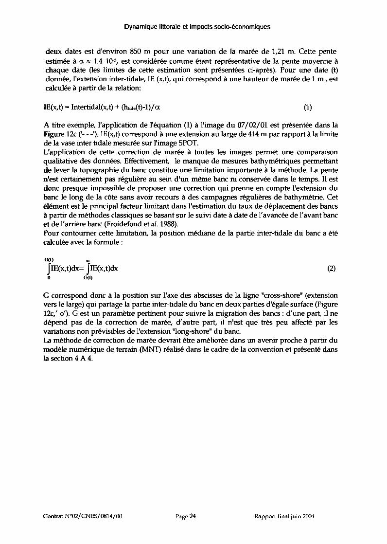
deux dates est d'environ 850 m pour une variation de la marée de 1,21 m. Cette penteestimée à a. R:i 1.4 1(}3, est considérée comme étant représentative de la pente moyenne àchaque date (les limites de cette estimation sont présentées ci-après). Pour une date (t)donnée, l'extension inter-tidale, lE (x.t), qui correspond à une hauteur de marée de 1 m , estcalculée à partir de la relation:
IE(x,t) =Intertidal(x,t) + (htide(t)-l)/a (1)
A titre exemple, l'application de l'équation (1) à l'image du 07/02/0l est présentée dans laFigure 12c ('- - -'). lE(x,t) correspond à une extension au large de 414 m par rapport à la limitede la vase inter tidale mesurée sur l'image SPOT.L'application de cette correction de marée à toutes les images permet une comparaisonqualitative des données. Effectivement, le manque de mesures bathymétriques permettantde lever la topographie du banc constitue une limitation importante à la méthode. La penten'est certainement pas régulière au sein d'un même banc ni conservée dans le temps. Il estdonc presque impossible de proposer une correction qui prenne en compte l'extension dubanc le long de la côte sans avoir recours à des campagnes régulières de bathymétrie. Cetélément est le principal facteur limitant dans l'estimation du taux de déplacement des bancsà partir de méthodes classiques se basant sur le suivi date à date de l'avancée de l'avant bancet de l'arrière banc (Froidefond et al. 1988).Pour contourner cette limitation, la position médiane de la partie inter-tidale du banc a étécalculée avec la formule:
G(t) co
IIE(x,t)dx= IIE(x,t)dxo G(t)
(2)
G correspond donc à la position sur l'axe des abscisses de la ligne "cross-shore" (extensionvers le large) qui partage la partie inter-tidale du banc en deux parties d'égale surface (Figure12c,' 0'). G est un paramètre pertinent pour suivre la migration des bancs : d'une part, il nedépend pas de la correction de marée, d'autre part, il n'est que très peu affecté par lesvariations non prévisibles de l'extension "long-shore" du banc.La méthode de correction de marée devrait être améliorée dans un avenir proche à partir dumodèle numérique de terrain (MNT) réalisé dans le cadre de la convention et présenté dansla section 4 A 4.
Contrat W02jCNFSj0814jOO Page 24 Rapport final juin 2004

Dynamique littorale et impacts socio-économiques
....... trait de COI- mangrove- Inlertlclalx xOz origin
UlM N22
3.35 3.4 3.45
x 105
3.15 3.2 3.25 3.3x..m. (m)
3.1
,ç(x
5.55
5.5
a 5.45 L------.JL-------.JL-------.JL-------.J~------'_------'_ ___'_ ___'_...:....J
x5.8
5.75
5.7
g5.65~
>:::> 5.6
5
- inlertidal- mangrovex xOzorlgln
43x (m)
2b 0:lE====::::!:.~____=:::::~__-'----_~~=:...d
n
5000 i-----.---.----.----.--;===:::c::=====;_1
4000
~3OO0
SN 2000
1000
4000
~2000
--le- intertldlllio G
43x(m)
2C Oi=====''===~__~_O_-----'------!t:==:....d
o
Figure 12 : Etapes de la standardisation des limites des thèmes mangrove et vase inter-tidale appliquésà l'image du 02/07/01. Les objets d'étude initialement dans une projection UTM (a) sont ensuiteramenés dans un nouveau repère (b) qui a pour origine le point (x) situé au nord-ouest de la carte (a)pour axe des absdsses les distances le long de la côte et en ordonnée la distance à la côte de la vaseintertidale. (c) présente la limite corrigée de l'effet de marée IE ainsi que G, position centrale de la vaseintertidale.
3) Représentation matricielleLa troisième étape consiste à projeter les données dans le système x,O,t. Toutes les datescorrigées des effets de marée sont reportées dans la Figure Sa. La matrice IE(x,t) offre unevision synoptique de la migration du banc vers le nord ouest de 1991 à 2002. A ce stade,l'analyse reste limitée puisque la matrice IE(x, t) n'est pas uniformément informée. Le tauxde non couverture qui représente environ 23 % de la matrice lE(x.t) est toutefoissuffisamment bien réparti (voir figure 13 a) pour permettre une interpolation numérique dela matrice. Le résultat de l'interpolation (qui utilise triangulation cubique de Delaunay) surles données dans une grille uniformément espacée constitue la dernière étape de la méthodematricielle. Son application est présentée dans la Figure 13 b.
Contrat W02jCNESj0814jOO Page 25 Rapport final juin 2004

Dynamique littorale et impacts socio-économiques
2005
4000
20003000
a1995 2000
1990 1000
01985 (m)
0 2 3 4 5 6x (m) x 10'
2005
40002000
b 3000
19952000
1990 1000
1985 1 00 2 3 4 5 6 (rn)
x(m) x 10'
Figure 13 : Représentation matricielle des résultats standardisés (a) et interpolés (b). Le dégradé decouleurs représente la distance à la côte de la vase inter-tidale.
Contrat W02/CNES/0814/00 Page 26 Rapport final juin 2004

Dynamique littorale et impactssocio-économiques
3 - CINETIQUE DU LITTORAL
Les résultats quantifient l'évolution spatio-temporelle des thèmes mangrove (depuis 1986) etvase intertidale (depuis 1991, date à laquelle apparaît le nouveau banc sur le littoral entreCayenne et Kourou)
A DYNAMIQUE COTIERE DE KOUROU
1) Cinétique du banc de vaseLa méthode matricielle peut être utilisée pour étudier les modifications de la mangrove et dela vase inter-tidale et plus généralement toutes les combinaisons mathématiques de ces deuxobjets d'étude. Parmi les combinaisons possibles qui peuvent être dérivées de la méthode, lasurface absolue de la vase émergée, estimée en soustrayant de la zone inter-tidale lasuperficie couverte de mangrove tel que:
IE'=lE-mangrove (3),
se révèle être le paramètre le plus pertinent pour le suivi de la migration des bancs.L'évolution spatio-temporelle de lE' est présentée dans la Figure 13 a. La maille de la matriceinterpolée est de 200 m en abscisse et de 300 jours en ordonnée. Parmi le jeu de donnéesdisponibles 9 dates conviennent pour une estimation directe de la localisation moyenne deG (rappeler (17/11/91, 16/10/95, 26/10/95, 28/09/96, 06/09/98, 07/02/00, 02/07/01,14/12/01, et 19/09/02). La migration de G, visible dans la Figure 13 a ('0'), est presquecontinue dans le temps à l'exception de la valeur au 16/10/95 qui est localisée dans la partiedroite de la matrice. Cette localisation est surprenante en comparaison à celle du 26/10/95(10 jours plus tard) qui est dans la tendance continue de l'ensemble des dates. Cettediscontinuité révèle les limites de la méthode d'estimation de la position du banc pour desimages acquises à des hauteurs de marée élevées (2.35m pour l'image du 16/10/95). Dans untel cas, la surface inter-tidale extraite des images est trop faible pour être représentative etl'estimation de G est imprécise. Cette observation nous a conduit à éliminer cette date pourl'interpolation. A l'exception de l'image du 17/11/91, les autres dates sont acquises à deshauteurs de marée suffisamment basses pour l'estimation de G (voir Tableau 2). L'image du17/11/91 est toutefois conservée puisqu'elle contient des informations cruciales relatives àl'arrivée du banc de vase sur le site d'étude.
L'équation (2) est appliquée à la matrice interpolée Œ'(x.t) afin de quantifier la positionmoyenne du banc pour une observation à une échelle de temps annuelle (Figure 14 a, '.').Les taux de migration du banc, calculés à partir des mesures directes et interpolées de G ('0'et '.', respectivement) sont représentés sur la Figure 14 b. La barre d'erreur associée à lavitesse interpolée correspond à la moyenne de l'écart type qui est dérivée des méthodesd'interpolation de la matrice, linéaire, cubique et V4 (Matlab 6.0.0.88 version ©).
Contrat N°02/CNES/0814/00 Page 27 Rapport final juin 2004

Dynamique littorale et impacts socio-économiques
20054000
20003000
.-..1995 E-- 2000N
1990 1000
1985a 0 2 3 4 5 6 (m )
x (m) x 10~
4000
3000 t- ï r-'~.. 1 1~
111
§.. 2000 1 11 - .,
>.1 ~:1:: ,... ._, ' -1G)
Qi 1 1--u 1000 1
11
1 1~ 1
1
b 0 t. .
1990 1992 1994 1996 1998 2000 2002 2004years
Figure 14 : a) Evolution spatio-temporelle de la zone inter-tidale du banc de Kourou (L'embouchuredu fleuve se situe autour de l'abscisse x=l2km).
b) Taux de migration estimés par mesures directes et indirectes.
Les taux de migration du banc de vase calculés à partir des mesures directes (voir Figure 14b) mettent en évidence trois tendances importantes:
de 1991 à 1996 le taux moyen est inférieur à 2 km/ anentre 1996 et 2000, le taux moyen est significativement supérieur puisqu'il atteint 2,5km/an ;puis, entre 2000 et 2002, le taux diminue pour être presque stoppé.
Dans le détail, et grâce à la haute résolution temporelle de la série d'image, des évènementssaisonniers peuvent également être observés. Ainsi, un pic de vitesse est enregistré à plus de3 km/ an entre octobre et décembre 2001. Contrairement au problème de correction de maréerencontré lors du traitement des images d'octobre 1995 (présenté juste au dessus), ce pic nepeut être lié aux limites de correction puisqu'il est déduit à partir d'images acquises à deshauteurs très similaires (1,44m. en octobre 2001 et 1,28 m en décembre 2(01).Cette accélération abrupte coïncide avec une arrivée précoce de la saison des plus forts ventsqui s'étend généralement entre décembre et mars. L'image du 14/12/01 montre une houleimportante déferlant sur une grande distance qui caractérise bien les conditionsexceptionnelles de forçage rencontrées cette année là.
Contrat W02/CNES/0814/00 Page 28 Rapport final juin 2004

Dynamique littorale et impacts socio-économiques
Ainsi, des événements très dynamiques peuvent se produire à l'échelle hebdomadaire ousaisonnière; il conviendra de mieux les comprendre, du fait de leur impact fort sur lesactivités de dragage.
Les taux de migration du banc de vase, calculés à partir des mesures interpolées, apportentdes informations complémentaires. Compte tenu de la résolution de 300 jours utilisée pourl'interpolation, les évènements saisonniers ne peuvent pas être observés. Par contre,l'interpolation permet de reconstituer des tendances qui échappent autrement aux mesures.C'est notamment le cas du ralentissement de 1994.Une importante extension "cross-shore" de la vase inter-tidale est visible sur les dernièresannées. La limite externe par rapport au trait de côte stable qui était à 2 km en 1995 est en2002 à 4 km. Cela se traduit par des teintes claires sur la matrice présentée sur la figure 14 a.Cette extension est corrélée au ralentissement enregistré entre 2000 et 2002.Ce ralentissement du banc, reporté dans la figure 14b, a probablement deux explications. Lapremière correspond au passage du banc dans une large baie formée dans la mangrove(Figure 15,"· - • •"). En comblant cette baie, le banc a probablement ralenti sa migration. Uneseconde explication implique la présence de nombreux hauts fonds rocheux à l'approche deKourou (Figure 15, '.'). Formant de véritables épis naturels, ces hauts fonds rocheuxsemblent avoir favorisé une extension vers le large du banc ralentissant sa progression lelong de la côte. La partie sub-tidale du banc a pu continuer sa progression vers le nord-ouesten dépit de la présence des épis. C'est ce que semble indiquer l'analyse de l'image du 5 août2002 (image 16 du Tableau 2). Sur cette image, les conditions d'acquisition révèlent une trèsforte corrélation entre la position des enrochements et un niveau de réflectance qui, selon lestravaux de Gratiot et al. (2003) correspond aux zones proches sub-tidales, sous uneprofondeur d'environ 1 mètre lors de l'acquisition.Cette hypothèse de basculement de la zone sub-tidale du banc sera discutée dans la dernièrepartie du rapport à la lumière des résultats obtenus dans le volet « opérationnel»
2km
Figure 15 : Caractéristiques morphologiques locales et chenal d'accès au port de Pariacabo (en fondimage SPOT du 05/08/2002). Les hauts fonds rocheux sont représentés par des étoiles noires. L'anseest visible au niveau de la route de Guatemala
Contrat N°02/CNES/0814/00 Page 29 Rapport final juin 2004
Dynamique littorale et impacts socio-économiques
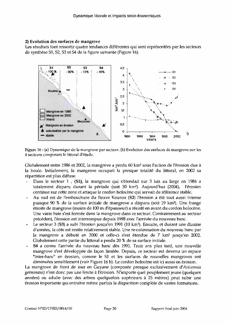
2) Evolution des surfaces de mangroveLes résultats font ressortir quatre tendances différentes qui sont représentées par les secteursde synthèse 51, 52, 53 et 54 de la figure suivante (Figure 16).
51 52 S3 54 4,5,-'.~~1 0V' -90% -18% -40% 514 \
\- -0- - 52
"' 13 ,5
\ ·· · · · .. · ·· · · 53l ! ..
KOUROù'tI.3 \ - ·_-. · · - -· 54
" \~E
2,5 ~
..lol: 2 ""'..... ....-.... )i
• ~ \~ ~. ~
D Mangrove en 1986 ..lol: 1,5 -.D Mangrove en 2002D Inland 1 ._ - - - . _ - ~ - -.- - - - - --~-.-._ -•MAcOURIA
~~j( Mangrove en érosion j( 0,5
• colonisation par la mangrove 0 ~
- stable a b1986 1990 1994 1998 2002
vears
Figure 16: (a) Dynamique de la mangrove par secteur, (b) Evolution des surfaces de mangrove sur les4 secteurs composant le littoral d'étude.
Globalement entre 1986 et 2002, la mangrove a perdu 60 km2 sous l'action de l'érosion due àla houle. Initialement, la mangrove occupait la presque totalité du littoral, en 2002 sarépartition est plus diffuse .
Dans le secteur 1 , (51), la mangrove qui s'étendait sur 3 km au large en 1986 atotalement disparu durant la période (soit 30 km-). Aujourd'hui (2004), l'érosioncontinue sur cette zone et attaque le cordon holocène qui servait de référence stable.Au sud est de l'embouchure du fleuve Kourou (52) l'érosion a été tout aussi intensepuisque 90 % de la surface initiale de mangrove a disparu (soit 19 km-). Une frangeétroite de mangrove (moins de 100 m d'épaisseur) a résisté en avant du cordon holocène.Une vaste baie s'est formée dans la mangrove dans ce secteur. Contrairement au secteurprécédent, l'érosion est interrompue depuis 1998 avec l'arrivée du nouveau banc.Le secteur 3 (53) a subi l'érosion jusqu'en 1991 (10 km-), Ensuite, et durant une dizained'années, la côte est restée relativement stable. Une re-colonisation du nouveau banc parla mangrove a débuté en 2000 et celle-ci s'est étendue de 7 km2 jusqu'en 2002.Globalement cette partie du littoral a perdu 20 % de sa surface initiale.54 a connu l'arrivée du nouveau banc dès 1991. Trois ans plus tard, une nouvellemangrove s'est développée de façon limitée . Depuis, ce secteur est devenu un espace"inter-banc" en érosion, comme le 51 et les surfaces de nouvelles mangroves ontdiminuées sensiblement (voir Figure 16 b). Lecordon holocène est ici aussi en érosion.
La mangrove de front de mer en Guyane (composée presque exclusivement d'Avicenniagerminans) n'est donc pas une limite à l'érosion. N'importe quel peuplement jeune (quelquesannées) ou adulte (avec des arbres quelquefois supérieurs à 25 mètres) peut subir uneérosion importante qui entraîne même parfois la disparition complète de vastes formations.
Contrat N°02/CNES/0814/00 Page 30 Rapport final juin 2004
Dynamique littorale et impacts socio-économiques
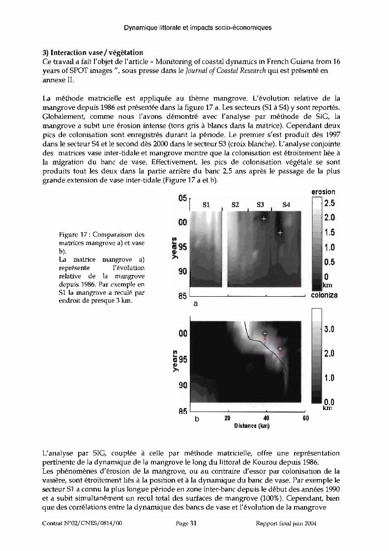
3) Interaction vase / végétationCe travail a fait l'objet de l'article « Monitoring of coastal dynarnics in French Guiana from 16years of SPOT images", sous presse dans le JournaL of CoastaL Research qui est présenté enannexe II.
La méthode matricielle est appliquée au thème mangrove. L'évolution relative de lamangrove depuis 1986 est présentée dans la figure 17 a. Les secteurs (51 à 54) Ysont reportés.Globalement, comme nous l'avons démontré avec l'analyse par méthode de SIG, lamangrove a subit une érosion intense (tons gris à blancs dans la matrice). Cependant deuxpics de colonisation sont enregistrés durant la période. Le premier s'est produit dès 1997dans le secteur 54 et le second dès 2000 dans le secteur 53 (croix blanche). L'analyse conjointedes matrices vase inter-tidale et mangrove montre que la colonisation est étroitement liée àla migration du banc de vase. Effectivement, les pics de colonisation végétale se sontproduits tout les deux dans la partie arrière du banc 2,5 ans après le passage de la plusgrande extension de vase inter-tidale (Figure 17 a et b).
L'analyse par SIG, couplée à celle par méthode matricielle, offre une représentationpertinente de la dynamique de la mangrove le long du littoral de Kourou depuis 1986.Les phénomènes d'érosion de la mangrove, ou au contraire d'essor par colonisation de lavasière, sont étroitement liés à la position et à la dynamique du banc de vase. Par exemple lesecteur 51 a connu la plus longue période en zone inter-banc depuis le début des années 1990et a subit simultanément un recul total des surfaces de mangrove (100%). Cependant, bienque des corrélations entre la dynamique des bancs de vase et l'évolution de la mangrove
Contrat W02jCNESj0814jOO Page 31 Rapport final juin 2004

Dynamique littorale et impactssocio-économiques
puissent être établies, l'influence de la première sur la seconde n'apparaît pas toujoursclairement. La mangrove et la vase inter-tidale sont régies par des processus physiques etbiologiques à différentes échelles spatiales et temporelles.La dynamique spatiale de la mangrove (colonisation ou érosion) s'opèreperpendiculairement à la côte alors que celle de la vase inter-tidale est soumise à unemigration le long du littoral. Tout cela sous l'influence des forçages par la houle, la marée etles courants côtiers. La période de 2,5 ans séparant le passage de l'extension maximale de lavase-intertidale du début de colonisation met en évidence les longues et complexesinteractions entre le banc de vase et la mangrove. L'extension cross-shore de la vase intertidale protège dans un premier temps la côte des actions de la houle, permettantl'initialisation des processus de consolidation de la vase. Ensuite, les graines d'Avicenniagerminans et de LaguncuLaria racemosa, transportées par les courants de marée et par lescriques, peuvent être déposées lors des grandes marée sur les zones de vase consolidée etainsi entamer les processus de colonisation de la vasière. La figure 18 ci-après schématise cesinteractions.
Figure 18 Schémaconceptuel des processus enjeux dans la colonisation desvasières par la mangrove.~ forçages océaniques(marée, houle et courant)sont à l'origine des processusdynamiques mais aussi destabilisation (colonisationvégétale) du banc.
1 marée
lconsolidation
g2.5 ans
transport
n
migration du banc
Les interactions entre le banc de vase et la dynamique de la mangrove apparaissent plusclairement en considérant indépendamment les espaces de bancs des espaces inter-bancs.Pour ce faire, nous avons distingué les zones (spatio-temporelle) envasées et non envasées àpartir de la matrice « vase» ( Figure 17b) puis nous avons examiné les processus d'érosionou de colonisation végétale sur ces deux zones. Cette analyse est donc réalisée en combinantles informations des matrices vase et végétation.Les résultats sont présentés dans la figure 19. Ils mettent en évidence l'existence de troispériodes distinctes.
Contrat W02/CNFS/0814/00 Page 32 Rapport final juin 2004

Dynamique littorale et impacts socio-économiques
-~~-02
Figure 19 Erosion et g .- interbanc 3colonisation sur les zones de c: bancbanc et d'inter banc. Les .e -0.1 -- -..- ...
résultats sont corrélés aux ~EROSION
'J -0 - >-
vitesses de migration du ii 0.0 Ebanc Cl) COLONISATION .:x.
>0
a, 0.1Iii 0E
1900 1985 1900 1995 LOO:)
- De 1986 à 1995 la mangrove a subit une intense érosion aussi bien en zone de banc qu'enzone d'inter-banc.- La période 1995 à 2001 a été très active aussi bien pour l'érosion dans les espaces inter-banc
que pour la colonisation sur le banc.- Enfin la colonisation du banc s'est interrompue en 2001 alors que l'érosion de la mangroves'est stabilisée à un taux moyen de 100 mètres par an en zone inter-banc (littoral du CSGessentiellement).Ces trois phases sont relativement bien corrélées avec les taux de migration du banc deKourou (trait de couleur bordeaux dans la figure 19) enregistrés préalablement. Cettecorrélation reflète bien l'interaction décrite schématiquement sur la figure 17 sans pourautant l'expliquer. En fait, il est nécessaire de considérer ces dynamiques simultanément aucontexte du forçage océanique. Cette approche est abordée dans la section 3 C après avoirprésenté la cinétique des autres bancs.
B -RESULTATS SUR LES AUTRES BANCS
L'étude de la cinétique côtière de la zone de Kourou a du être complétée par celle d'autresbancs de Guyane; ceci afin d'estimer le rôle des paramètres locaux tels que les baies,l'orientation de la côte ou les emochements. La base de donnée réalisée pour l'étude couvrela quasi totalité du littoral guyanais avec des images depuis 1986.
1) Commentaires générauxLa méthode matricielle a été appliquée à l'ensemble des images disponibles. Elle fourniequatre matrices régionales.
4000
3000
2000
1000
o87632o
2000
1990
"'<;~ 1995
4 5X(UTM)
Figure 20: Evolution spatio-temporelle de la vase inter-tidale dans la région de Kaw
Les résultats sur le site de Kaw, présentés sur la Figure 20, sont difficilement exploitables.L'absence de données entre 1991 et 1998 limite les possibilités d'interpolation de la matrice.Par ailleurs, cinq des huit images satellites sont acquises à des hauteurs de marée supérieures
Contrat W02/CNFS/0814/00 Page 33 Rapport final juin 2004

Dynamique littorale et impacts socio-économiques
à deux mètres; les corrections de marée apportées dans la méthode sont probablementinsuffisantes.
Dans la figure 21, les trois autres matrices régionales sont assemblées les unes aux autres.Comme les sites sont contigus, elles couvrent sans discontinuité environ 180 kilomètres delittoral. Cette figure fournie donc une vision complète de la dynamique du littoral à partirde laquelle différents résultats peuvent être déduits.
Mana Organabo Iracoubo Sinnamary CSG Kourou/ Macouria
Figure 21 : Assemblage des matrices de vase inter-tidale de l'ouest de Cayenne jusqu'à Mana.
2) Le rôle de l'orientation de la côteJusqu'à Iracoubo, les bancs de Kourou et de Sinnamary sont séparés par des espaces interbancs s'étendant sur 25 à 30 km. Les zones inter-tidales sont particulièrement développéesavec des extensions au large atteignant fréquement plus de 3km, jusqu'à 4 km notammentsur le banc de Kourou à partir de 1997. La grande barre rouge sur l'estuaire de l'Iracoubo,tout comme celle qui se devine au niveau de Mana, ne doit pas être prise en considération. Ils'agit d'artefacts liés à la migration des bancs au droit des estuaires majeurs.Au delà d'Iracoubo, les bancs se resserrent, les distances inter-bancs atteignant en moyenne10 km. Dans cette partie, les bancs sont beaucoup moins étendus au large, 2.0 à 2.5 km aumaximum.Le changement d'orientation de la côte, qui se produit entre les embouchures des fleuvesSinnamary et Iracoubo, est certainement à l'origine de la modification de cette dynamique dulittoral. D'une part, il s'agit certainement du seul facteur évoluant si distinctement et restantconstant à l'échelle de plusieurs dizaines de kilomètres; d'autre part, cette observation est encohérence avec les résultats d'études menées au Surinam (Augustinus, 1987). Lamodification d'angle de la côte est sans nul doute un facteur d'accélération du transportlongshore, sous l'action des houles. Effectivement, un angle d'attaque des côtes par la houleplus ouvert favorisera un étirement des bancs le long de la côte.
3) Le rôle des estuairesLes estuaires de Kourou et de Sinnamary présentent deux cas de figures intéressants. Ils sontreprésentés tout les deux par des petites barres verticale blanches dans la figure 21.Pour le site de Kourou, la partie inter-tidale du banc ne s'est pas encore fixée de l'autre côtéde l'estuaire; des passages de vase peuvent donc avoir lieu et ponctuellement envaser leszones de plages de Kourou, mais jusqu'à présent il n'y a pas eu d'arrivage massif qui auraitpu se fixer. Le débit du fleuve reste pour l'heure suffisant pour entraver la formation dezone de slikke à l'ouest. Notons que les actions de dragages contribuent également à cetentravement par la liquéfaction et la remobilisation quotidienne des vases en transit dans lechenal.Sur le site de Sinnamary, deux étapes de franchissement de l'estuaire se sont produites.Autour de 1997-1998, un premier arrivage massif de vase est venu s'accoler sur la rivegauche de l'embouchure. Il correspond probablement au passage d'un lac de vase tel que
Contrat N °02/CNES/0814/00 Page 34 Rapport final juin 2004

Dynamique littorale et impacts socio-économiques
schématisé dans la figure 4. Constitué de vase faiblement consolidée, cette accumulation aensuite été re-mobilisée et dissipée dans le transit littoral sous l'action du forçage océanique.Ceci explique sa disparition brutale avant 2000. A partir de 2001, la vase franchit en forcel'estuaire. Compte tenu de la quantité de vase, le fleuve n'est plus compétent pour assurerson rôle de chasse.
4) Des vitesses de déplacement homogènesAfin d'estimer des vitesses globales de déplacement des bancs sur tout ce littoral, des traitsnoirs sont tracés en diagonal sur les matrices de la figure 21. Ces repères représentent unedistance de 20 kilomètres sur une durée de 10 ans. Une analyse visuelle de la figure sembleconfirmer que les vitesses moyennes des bancs sur ces 17 années sont de l'ordre de 2kilomètres par an. Le banc de Kourou reste celui qui a connu les vitesses de déplacement lesplus importantes.A ce stade de l'analyse, le rôle des hauts fonds et battures ne peut pas encore être clairementdéfini.
C - ROLE DES FORÇAGES EXTERNES
Ce travail a fait l'objet de l'article « Atlantic trade-wind waves and mud bank dynamics onthe French Guiana coast, South America", soumis à la revue Marine Geology et qui estprésenté en annexe III.
Nous avons indiqué auparavant la nécessité de considérer les forçages externes pourcomprendre les dynamiques en interaction des bancs de vase et de la mangrove. Lesprincipaux forçages océaniques sont ceux générés par les courants de marée, les courantscôtiers et la houle. En Guyane, le manque de moyens instrumentaux et de données limitentconsidérablement les possibilités d'étude du rôle des forçages océaniques. Ainsi, nous nedisposons ni de courantomètre ni de houlographe dans la zone côtière proche. L'étudeprésentée ci dessous repose sur l'acquisition de données de vents locaux et de vents globaux,à l'échelle d'environ l<XlOkm au droit de la Guyane, dans l'océan Atlantique tropical. Cesdonnées ont été traitées afin d'estimer les caractéristiques des houles qui atteignent la zonelittoral.La méthode de traitement des données de vents est rappelée brièvement avant de présenterl'impact indirect du vent, via les houles, sur la migration des bancs.
1) Génération des houles par le vent, généralitésLa formation de la houle par le vent est due à des fluctuations de la pression atmosphériqueà l'interface entre l'océan et l'air, ainsi qu'à un mécanisme de couplage entre les vagues et levent : le vent proche de la surface est modifié par la présence des vagues, et cettemodification entraîne une amplification des vagues.
En faisant l'hypothèse d'un état de mer totalement développé, en considérant que le ventsouffle à une vitesse constante U sur une zone de fetch d'une longueur X durant un certaintemps, la période et la hauteur de la houle augmenteront avec U et X selon Hasselmann et al.(1973):
Contrat N°02/CNFS/0814/00 Page 35 Rapport final juin 2004

Dynamique littorale et impactssocio-économiques
(4.a)
(4.b)
où Hoest la hauteur de la houle (m), Tp le pic de fréquence du spectre de houle JONSWAP(s), X la distance sur laquelle le vent souffle a une vitesse et dans une direction constante (m),g l'accélération gravitationnelle (m.ss), U la vitesse du vent mesurée à 10 mètres au dessusdu niveau de la mer (m.si), Cl et C2 des constantes dérivées de données de houle collectéeslors de la campagne JONSWAP (Hasselmann et al., 1973), respectivement 1.6x1Q-3 et285.3xlQ-3.
Les équations 4a et 4b indiquent que l'augmentation de la hauteur de la houle estprincipalement dépendante de la vitesse du vent alors que la période de la houle est affectéeaussi bien par la vitesse du vent que par la longueur de la zone de fetch (région où le ventsouffle avec une intensité et une direction constantes).L'hypothèse d'un état de mer totalement développé est généralement satisfaite pour deshoules générées sur une zone de fetch locale, ainsi les équations la et lb sont vérifiées. Pourdes zones de fetch plus larges (océaniques), le temps durant lequel souffle le vent peutdevenir un facteur limitant et doit être pris en compte. Le vent devra souffler durant unepériode suffisamment longue pour stresser les houles durant leur propagation sur la zone defetch,
2) Caractéristiques des vents locaux et globauxDurant les 30 dernières années, les vents enregistrés aussi bien localement (Météo-France)que régionalement, à l'échelle de l'Atlantique tropical (pseudo-stress de vent de J. Servain :http:j jwww.coaps.fsu.edujWOCEjhtnùjatlmonyr.htnù) montrent des tendancessaisonnières bien marquées.
Servcin's Atl"nti c Pse udo-Stress vectors April 2000
EQ
las
COM'SjFSU 0 10 20 30 40 50 60 70 ao 90 100 M' s- ORSTOM
Figure 22: carte des pseudo stress de vent du mois d'avril 2000 de J. Servain
L'analyse des données de vents régionaux s'est faite, à partir des données de pseudo-stressde vent en déterminant la zone de fetch à considérer pour la génération des houles sur lescôtes de Guyane Française. L'aspect technique d'extraction des intensités de vents à partirdes matrices mensuelles, tel que celle présentée ci dessus, est détaillée dans l'annexe 111.
Contrat W02/CNES/0814/00 Page 36 Rapport final juin 2004

Dynamique littorale et impacts socio-économiques
De janvier à mai, les vents présentent une intensité nettement supérieure à ceux de juillet àoctobre, signe d'une fluctuation saisonnière prononcée. Des fluctuations multi-annuellespeuvent aussi être enregistrées en fonction de l'échelle d'observation. Les vents côtierslocaux mesurés à l'Ile du Diable depuis 1975 sont en constante perte d'intensité (voir figure)alors que les vents synoptiques, déduits des mesures depuis 1964, augmentent globalement,avec une légère diminution de leur intensité dans les années 1980 (Voir Figure 23).
2005 2005.----~--_,_------.----,..-----,
10986
....~ .
.. .. .~ ' "
1990
1995
1975
2000
1960 L _ _ --'--__~_______L_ _ =.::::::::::=:::::J5
1965
1970
1985l!'
'"(l)>- 1980
9
-er- lan-may-e- annual-v- lull-ocl
5 6
Wind speed (m.~)
43
2000
1965
1990
1995
1970
1975
!! 1985..Il
~19B0
7
Uf(m s·l)
Figure 23 (a) Fluctuations inter-annuelles des vents locaux de puis 1975 aux nes du Salut (ne duDiable, station Météo France). (b) Fluctuations inter annuelles des vitesses de vent champs large sur lazone de fetch depuis 1964 (données J. Servain)
L'application des équations 4 sur les données de vents locaux et synoptiques a permis dedéduire les caractéristiques de houle élémentaires, à savoir la hauteur moyenne et la périodeprincipale. Pour des raisons décrites dans l'article présenté en Annexe 3, les informationsobtenus ne permettent qu'une analyse qualitative du rôle des houles sur la migration desbancs.
3) Forçages et migration des bancsNous adoptons l'hypothèse proposée par Rodriguez et Mehta (1995) selon laquelle l'impactindirect du vent sur la migration des bancs (via les houles générées) résulte du transport desvases fluidifiées par les houles en cours d'amortissement. Selon cette hypothèse, la vitesse demigration des bancs est proportionnelle au paramètre H3/Tp2 (ratio entre une hauteurcaractéristique de houle océanique H et une période caractéristique de houle T). L'évolutiontemporelle de ce paramètre est représentée sur la Figure 24 c et est comparée aux principauxparamètres de la dynamique côtière. Les houles générées localement ne semblent pas jouerun rôle significatif dans le déplacement des bancs et le paramètre H3/Tp2 déduit des ventslocaux est cinq a dix fois plus faible que celui déduit des vents synoptiques. Cependant ceshoules générées localement peuvent jouer un rôle dans l'érosion de la mangrove côtière, bienplus important que les vagues océaniques qui sont amorties rapidement en périphérie desbancs.
Contrat W02jCNESj0814jOO Page 37 Rapport final juin 2004

Dynamique littorale et impactssocio-économiques
e,
b.
.".~ 60 · .'-' .c:.!! --! 4-.0 ···· · · ··· · ·· ··L l '-'=-=-,..:~~,:..;:.;:.~:.:..:.L...,...,..,....DlI --
E~ 2.0 .. - ---.Cl - ---a~eo
1960 1965 1970 1975 1960 1985 1990 1995 2000 2005
~ -0.2 r;:::====::::::::==:::;--....----....----:7\-i
~ -0.1 1-= :::'''' 1.;"'S,;Nu~ u
g 0.0 . - - . . - - \ . . '" .CIl COLONISATION J 1~ 0.1 \ .
~ LIII -0.2 I....-__~ '--__--'- ---..JE 1960 1970 1980 1990 2000
~EC
.!2.. 0.6 .N
~'1 0.4 " '. ' - . ' b.' .6.~ 6. ~
~~ 0.2 Zl.a Ll.
A
(b) Migration des bancs de vasesur le littoral de Kourou entre1960 et 2002
Figure 24:Evolution géomorphologique du
littoral de Kourou et forçage parla houle(a) Evolution cross-shore de lamangrove entre 1990 et 2002(Gardel et Gratiot sous presse b);
(c) Evolution des paramètres deforçage par la houle des ventslocaux et synoptiques depuis1%4.
200019901980yeats
1970O'--------'----'------'----~---..J
1960
Par contre, la Figure 24 montre une certaine corrélation entre la vitesse de migration du bancde Kourou d'une part et le paramètre de forçage par le vent synoptique d'autre part. Ainsi,les deux épisodes de faible vitesse de migration, observés de 1950 à 1970 puis de 1979 à 1984(Figure 24b) correspondent bien à des épisodes ou le paramètre de forçage est moinsimportant.
4) Perspectives de recherche sur l'action des houles dans la structuration côtièreEnfin, pour le moment, il n'est pas envisageable de prédire de façon quantitative lamigration des bancs. Effectivement, les vents mensuels utilisés ici ne permettent pas dedécrire de façon appropriée les interactions houle/ migration des bancs. Des résolutionsjournalières seraient plus pertinentes pour étudier les effets de seuil du forçage par la houleet les modifications rhéologiques des bancs de vase associées. Dans l'avenir, l'effort devraêtre mis sur l'intégration de données de vents quotidiennes ou bien directement surl'utilisation de modèles de houle pour considérer la dynamique côtière à une échelle pluslarge. Ces actions devraient permettre d'identifier et de comprendre le rôle des variabilités àgrande échelle sur la morphologie côtière et le rôle des particularités géomorphologiqueslocales dans la migration et la dynamique des bancs de vase.
Contrat W02/CNF5/0814/00 Page 38 Rapport final juin 2004

Dynamique littorale et impactssocio-économiques
~ - CARACTERISATION DU BANC ET EVOLUTION DE L'EFFORT DE DRAGAGE
L'objectif de ce volet est de comprendre l'évolution de l'envasement du chenal d'accès auport de Pariacabo par rapport à l'évolution spatio-temporelle du banc de vase. L'effort dedragage depuis 2000 n'a cessé de progresser (voir figure 1) vers le large signe d'uneprogression vers le large de la zone sub-tidale alors que la partie inter-tidale du banc s'eststabilisée à partir de cette date, comme le montre les résultats de la méthode matricielleappliquée au banc de Kourou (Figure 14).
Nous avons vu qu'un banc de vase était constitué de plusieurs éléments plus ou moinsdynamique (voir figure 4). La partie inter-tidale du banc que nous avons suivie pourquantifier la cinétique du littoral de Kourou n'a pas le même comportement spatio-temporelque la partie sub-tidale dont nous avons peu de connaissances (partie immergée du banc). Orcette partie sub-tidale du banc de Kourou est celle qui contribue actuellement activement àl'envasement du chenal.Nous avons donc entrepris de caractériser le banc de Kourou dans ces parties intertidales etsub-tidales afin de comprendre l'évolution de l'effort de dragage du chenal. Pour ce faire,deux actions distinctes utilisant des méthodes complémentaires ont été entreprises.La première action vise à caractériser la topographie de la zone inter-tidale en utilisant unesérie d'images SPOT acquises dans un intervalle d'un mois durant la saison sèche 2003 à deshauteurs de marée différentes. Cette action, couplée à des mesures ponctuelles deconcentration des sédiments, permet de diagnostiquer la dynamique morpho-sédimentaireactuelle de cet espace.La seconde action vise à délimiter la zone sub-tidale par des mesures de bathymétrie et deconcentration en sédiment du banc. Cette action a fait l'objet d'une campagne en mer le 15avril 2003 à bord d'une embarcation de la société Atlantique Dragage.
A CARACTERISATION DE LA PARTIE INTER-TIDALE DU BANC
1) Données utiliséesUne série de 5 images SPOT a été acquise dans le cadre de la convention grâce à un bon ISIS.Ces images SPOT 5 et SPOT 4 sont acquises durant la saison sèche 2003 (sur un mois) àdifférentes hauteurs de marée. Nous faisons l'hypothèse que durant la saison sèche, lesforçages hydrodynamiques sont faibles et que l'évolution géomorphologique du banc et enparticulier la zone intertidale est relativement stable.Dans l'hypothèse d'un écoulement quasi hydrostatique, le but est de se servir de la limiteeau/vase sur les images comme d'une courbe de niveau correspondant à la hauteur demarée prédite par le SHOM.Les images utilisées sont:
date Hm (SHOM) Sato Bandes Spectr Origine13 août 2003 0,87 SPOT 510m MIR-PIR-R-V Bon ISIS29 août 2003 0,91 SPOT 510m MIR-PlR-R-V Bon ISIS30 août 2003 1,12 SPOT42Om MIR-PIR-R-V PNEC8 sept 2003 1,3 SPOT 510m MIR-PIR-R-V Bon ISIS15 sept 2003 1,68 SPOT42Om MIR-PIR-R-V Bon ISIS19 sept 2003 2,21 SPOT 510m MIR-PIR-R-V Bon ISIS
Table 3: liste des images acquise en été 2003 et leurs caractéristiques. Les hauteurs de maréecorrespondantes (en mètres) sont indiquées.
Contrat W02jCNESj0814jOO Page 39 Rapport final juin 2004

Dynamique littorale et impacts socio-économiques
Figure 25 : les 6 images SPOT utilisées pour caractériser la topographie de la zone inter-tidale du bancde Kourou.
2) Méthodes d'extractionLes images, acquises au format 1B ont été géo-référencées puis informées dans le systèmeWGS84, UTM Nord 22. La zone d'étude est extraite des images. Les nouvelles imagescouvrent une surface de 30*30 km.L'objectif principal est d'extraire une image binaire de la vase intertidale. Dans cetteperspective, diverses méthodes ont été développées, testées et adaptées jusqu'à l'obtentionde résultats satisfaisants. Dans un premier temps, des segmentations sont opérées sur lesimages afin de leur soustraire l'ensemble des surfaces n'appartenant pas au thème vaseintertidale (végétation, eau ... ). Des masques sont obtenus par l'application d'algorithmes declassification non supervisée. Les classes regroupant le thème vase sont conservées, les autressont écartées et masquées. Dans les segments sélectionnés le processus est répété de façonitérative et interactive jusqu'a identifier les surfaces de vase intertidale correspondants à desétats de surface différents de vase exondées (crème, consolidée, phyto-benthos...).Des classifications en mode supervisé utilisant des parcelles d'apprentissage sur le terrain nesont pas envisageable sur des espaces aussi dynamiques que les zone inter-tidales,Effectivement, d'une marée à une autre et en fonction de la durée d'exondation, la mêmesurface de vase pourra avoir des radiométries très différentes.Pour obtenir les images binaires, les classes sont regroupées dans une unique classe de vaseexondée. Les images binaires sont alors vectorisées de manière à obtenir pour chaque dateune courbe de niveau correspondant à la hauteur de marée (modèle du SHOM). Ces courbessont présentées dans la figure ci-après (Figure 26).
Contrat W02jCNESj0814jOO Page 40 Rapport final juin 2004
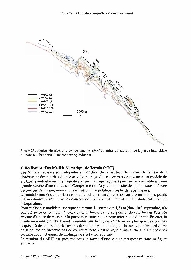
Dynamique littorale et impactssocio-économiques
13/08/03 0,8729/08/03 0,91
30/08/03 1,1208/09/03 1,3015/09/03 1,6819/09/03 2,21
~o
Figure 26: courbes de niveau issues des images SPOT délimitant l'extension de la partie inter-tidaledu banc aux hauteurs de marée correspondantes.
4) Réalisation d'un Modèle Numérique de Terrain (MNT)Les fichiers vecteurs sont étiquetés en fonction de la hauteur de marée. Ils représententdorénavant des courbes de niveaux. Le passage de ces courbes de niveau à un modèle desurface (éventuellement représenté par un maillage régulier) peut se faire en utilisant unegrande variété d'interpolateurs. Compte tenu de la grande densité des points sous la formede courbes de niveau, nous avons utilisé un interpolateur simple, de type linéaire.Le modèle numérique de terrain obtenu est donc un modèle de surface où tous les pointsintermédiaires situés entre les courbes de niveaux ont une valeur d'altitude calculée parinterpolation.Pour réaliser ce modèle numérique de terrain, la courbe des l,3D m (date du 8 septembre) n'apas été prise en compte. A cette date, la limite eau-vase permet de discriminer l'arrivéerécente d'un lac de vase, sur la partie nord-ouest de la zone inter-tidale du banc. En effet, lalimite eau-vase (courbe bleue) présentée sur la figure 27 découvre plus que des courbesacquises à des dates antérieures et à des hauteurs de marée plus basse. La limite nord-ouestde la courbe ne présente pas de courbure forte, c'est le signe d'une surface très plane danslaquelle aucun chenaux de drainage ne s'est encore formé.Le résultat du MNT est présenté sous la forme d'une vue en perspective dans la figuresuivante.
Contrat N °02jCNESj0814jOO Page 41 Rapport final juin 2004

Dynamique littorale et impactssocio-économiques
Kourou
z(m)2.2
2
1.8 ~N
1.6
1.4
1.2
Figure 27: vue en perspective du MNT de la zone inter-tidale du banc de Macouria. Cette vue permetde mettre en évidence la topographie des différents secteurs de la zone:- Le secteur (1) correspond à l'arrière du banc. Cet espace subit une érosion intense. Le profiltopographique est ainsi relativement abrupte (les courbes de niveau sont rapprochées).- Le secteur (2) correspond à la zone où la vase inter-tidale s' étend le plus au large. De nombreuxchenaux de marée découpent la surface dont la pente est nettement plus douce. C'est id que sedéveloppent des spot de colonisation végétale sur les zones de barres ou le long des chenaux demarée.- Le secteur (3) situé en avant du banc a quant à lui une surface de pente très douce. C'est un espace d'accrétionvaseuse qui correspond à un lac de vase. Au delà de ce secteur, l'estuaire du fleuve Kourou.
Contrat W02jCNESj0814jOO Page 42 Rapport final ju in 2004

Dynamique littorale et impacts socio-économiques
B CARACTERISATION DE LA PARTIE SUB-TIDALE DU BANC
Dans le rapport intermédiaire nous faisions des hypothèses sur la morphologie du banc, sadynamique spatio-temporelle et sur son impact sur révolution de l'effort de dragage. L'effortde dragage du chenal s'opérant de plus en plus au large (pk 8 en 2000, pk 13.2 en 2004) nousvoulions avoir une idée objective de la limite du banc. Il est important de rappeler ici quecette limite n'est pas détectable à partir de données d'observation de la Terre et que seulesdes mesures in situ le permettent (Figure 28).
••
Figure 28 : Limite hypothétiquede la zone sub-tidale. Présentéelors de la présentation orale demi-étape au CSG. .,
. ! III ~lIIItIl.. 1I ,IIl:fl ~r.., ~'.t"lJ
::'. .. .. . ".:. .
.....................................
Une campagne de mesure de terrain a donc été initiée, en partenariat avec AtlantiqueDragage (société qui a en charge le dragage du chenal) , afin d'acquérir les donnéesnécessaires à une délimitation du banc de Kourou. L'objectif de la campagne du 15 avril 2004était de caractériser la partie sub-tidale du banc à proximité du chenal par des mesures debathymétrie mais aussi de concentration du lit en sédiments. A partir de campagnes deterrain réalisées dans la zone littoral entre Cayenne et Kaw, Cratiot et al. (2003) ont pu établirune limite franche entre les zones de bancs et les zones d'inter-bancs; limite caractérisée parun saut de concentration au delà de la valeur de 650 g/l en zone d'inter-bancs. Dans le mêmetemps, les zones de bancs étaient toujours caractérisées par des concentrations plus faibles,voisine de 550 g/l.
Il est important de rappeler que c'est à cette saison que les transports sédimentaires sont lesplus importants. Les résultats obtenus devront être confirmés et réactualisés par une autrecampagne réalisée en saison sèche.
1) Matériels et méthodesAtlantique dragage a mis a disposition une pilotine, son pilote ainsi que le responsable desactions de dragage, M. C Heidekamp. L'embarcation est utilisée habituellement pour réaliserles relevés bathymétriques bi-hebdomadaires du chenal. Elle est équipée d'un échosondeurbi-fréquence, d'un récepteur DCPS et reçoit en temps réelles données marégraphiques de laPointe des Roches (voir Figure 29). Ces données sont intégrées dans le logiciel d'AtlantiqueDragage qui restitue alors une bathymétrie absolue sur la route de navigation préenregistrée. Les données acquises en dehors du trajet du plan de route ne peuvent pas êtreexploitées.Côté IRD, nous disposions d'une benne de prélèvement permettant de récolter les sédimentsde surface du lit (cf. photographies Figure 29b).
Contrat W02jCNESj0814jOO Page 43 Rapport final juin 2004

Dynamique littorale et impactssocio-économiques
Figure 29: photographies du matériel utilisé. a) instruments à bord de la pilotine b) benne manuelutilisée pour les prélèvements de vase.
Un plan de route couvrant la zone proche du chenal a été établi sachant toutefois que lesprélèvements pouvaient se continuer plus au large, si la limite vase fluide/vase dure n'étaitpas trouvée.Lors de la campagne, nous avons réalisé 25 prélèvements de sédiments (une campagneantérieure, réalisée dans le cadre du Programme National d'Environnement Côtier avaitpermis de réaliser des prélèvements, 28 au total, plus proches de la côte)Au regard des premiers prélèvements, nous avons décidé d'étendre les transects au delà desroutes programmées initialement afin d'obtenir des vases indurées, significatives d'une zonehors banc. Effectivement la vase molle s'étendait nettement plus loin que ce à quoi nous nousattendions, au delà des Iles du Salut.
2) Traitements réalisésBathymétrieLes données de bathymétrie sont traitées par un logiciel propre à Atlantique Dragage qui estintégré dans le système de navigation. Atlantique Dragage nous a donc fourni un relevépapier des relevés bathymétriques sur les transects programmés.
Concentra tionConcernant les prélèvements sédimentaires, il s'agissait d'en extraire des taux deconcentration. Les caractérisations des sédiments de surface réalisées lors de la campagnerepose sur un protocole utilisé précédemment pour la caractérisation des zones proche subtidales de la bande côtière de Kaw (Gratiot et aL., 2003).Les échantillons sont ensuite séchés dans une étuve ventilée à 60°C pendant 72 heures. Lepesage des échantillons avant et après séchage permet d'obtenir la teneur en eau; laconcentration en matière sèche est alors déduite à partir de l'équation:
C(g/l)=Msed~ M sec (5)Vrol Mw +Msed
pw psavec C: la concentration en matière sèche (kg/ mè), Msed : la masse sèche de sédiment (kg),V/Dt: le volume total de l'échantillon (ms), M sec : la masse de l'échantillon après séchage (kg),Mw: la masse d'eau (kg), p wet p «: les masses volumique de l'eau et du sédiments,respectivement (kg/ mè).L'estimation de C à partir de (5) ne considère pas l'influence de la salinité, non mesurée dansle cadre de la campagne de mesure. Toutefois, cette influence reste limitée puisque elle induitune surestimation des mesures de l'ordre de 3%.
Contrat W02/CNFS/0814/00 Page 44 Rapport final juin 2004

Dynamique littorale et impacts socio-économiques
coordonnées UTMc(gll)
coordonnées UTMc(g/l)
coordonnées UTMc(g/l)
X y X Y X Y
1 323804 576886 502,8 20 331123 574207 662,3 38 330938 562359 734,8
2 324130 577859 496,0 21 331616 576320 609,8 39 332209 561300 624,6
3 324448 578794 513,6 22 332498 578283 628,6 40 333612 559359 627,34 324853 579699 557,1 23 332874 580474 618,3 41 334837 558271 701,26 325160 580658 544,0 24 323121 575117 521,0 42 331030 561784 588,1
7 325540 581558 560,2 25 322447 573264 531,9 43 330874 561730 605,0
8 325873 582543 541,2 26 320961 571334 512,4 44 329990 562836 674,39 326247 583508 609,2 27 322571 571331 537,2 45 329799 562699 625,210 326590 584472 414,4 28 324747 571124 484,1 46 328418 564911 595,911 329906 583174 619,0 29 324706 570868 543,9 47 327713 564424 586,412 329470 582256 657,0 30 325571 570050 602,7 48 327156 565577 597,313 329242 581308 660,0 31 326268 569355 628,8 49 326149 568858 597,414 328914 580337 544,6 32 326948 568062 788,7 50 324736 568078 662,615 328257 578443 512,2 33 328043 567209 627,8 51 324171 567678 587,316 327588 576547 578,9 34 329270 566099 708,4 52 323574 569673 668,017 326564 573714 636,9 35 328848 565865 635,7 53 323209 568651 550,7
18 325728 571190 607,7 36 330049 564992 628,2 54 322955 567429 623,119 330454 572146 668,3 37 329848 564729 651,9
Tableau 4 : points de prélèvement et taux de concentration en sédiments
Cartographies : bathymétrie et concentration en sédiment.Les données ponctuelles de bathymétrie et de concentration en sédiments sont interpoléesobtenir des cartes d'isobathes (Figure 30) et d'iso-concentration en sédiments (Figure 31)présentées ci-après.
IlesduCP Salut
FiRUIe 30 : carte de la bathymétrie « Atlantique Dragage », En rouge, les transects programmés surlesqu els les points sont enregistrés. Les iso-bathes sont ensuite calculées par interpolation.
Contrat W02jCNESj0814jOO Page 45 Rapport final juin 2004

Dynamique littorale et impacts socio-économiques
\,
Figure 31 : carte des concentrations en sédiments à la surface de la zone sub-tidale. En rouge, lespoints de prélèvements. La courbe des 650g/1 (en pointillé) est considérée comme la limite du banc.
3) RésultatsEn terme de bathymétrie, une zone relativement de très faible pente (0,6 rn/km) sedéveloppe dans la partie centrale cartographiée. Un changement de pente se produit autourde l'isobathe 5 m et l'extension du banc plus au large s'effectue avec une pente moyenne de1,5 rn/km qui reste relativement faible aussi.D'un point de vue sédimentaire, l'extension sub-tidale du banc de Kourou (concentrationinférieure à 650g/l) est fortement excentrée vers le nord-ouest par rapport à la zone intertidale. Elle présente également une extension au large très importante au delà des Iles duSalut ou les derniers relevés ont été effectuées. Cette extension est cohérente avec l'avancéepermanente de l'effort de dragage vers le large depuis 2000.La synthèse des résultats est présentée dans la figure ci-après (Figure 32). Notons bien quecette synthèse correspond à l'association de deux séries de mesures non simultanées. D'unepart un MNT de la zone intertidale estimé à partir de données satellites acquises en automne2003 et d'autre part, une campagne de mesure réalisée le 15 avril 2004. Un survol de la zonelittoral avait été programmé pour le mois de juin 2004 afin d'actualiser les analyses defonctionnement de la zone intertidale. Malheureusement, le plan Vigi-pirate a amené àdéprogrammer cette acquisition de nouvelles photographies aériennes.
Contrat N°02jCNESj0814jOO Page 46 Rapport final juin 2004
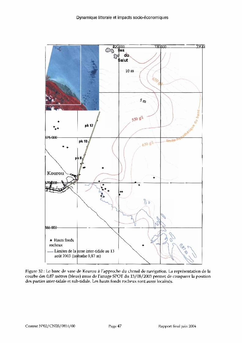
Dynamique littoraleet impacts socio-économiques
/
••
lOlll
++
1esdÙ
alut
•"..
'..
( (', 1
. ))~-_ /
• •
•+••
* Hauts fondsrocheux
- Limites de la one inter-tidale au 13août 2003 (is bathe 0,87 m)
Figure 32 : Le banc de vase de Kourou à l'approche du chenal de navigation. La représentation de lacourbe des 0,87 mètres (bleue) issue de l'image SPOT du 13/08/2003 permet de comparer la positiondes parties inter-tidale et sub-tidale. Les hauts fonds rocheux sont aussi localisés.
Contrat N°02jCNF5j0814jOO Page 47 Rapport final juin 2004

Dynamique littorale et impacts socio-économiques
c- BYPOTHESES DE FONCTIONNEMENT
Les résultats obtenus confirment les hypothèses que nous formulions lors du compte rendude mi-étape. Il y a bien eut un ralentissement du banc à la côte (zone inter-tidale) lié à l'effetcombiné d'une anse dans la mangrove (au niveau de Guatemala) et de hauts fonds rocheux.Alors que la vitesse de migration de la zone intertidale atteignait 2,7 km/ an entre 1995 et2000 (figure 33, phase 1), un fort ralentissement s'est produit à partir de 2000 (1,5 km/ an)jusqu'à une stabilisation de la zone depuis 2002. Arrivant au niveau de cette grande anse, lapartie inter-tidale du banc a ralentit en comblant ce décrochement naturel (figure 33, phase2). Formant de véritables épis naturels, les hauts fonds rocheux ont favorisé une extensionvers le large du banc ralentissant sa progression le long de la côte (figure 33, phase 3).Toutefois des passages de vase fluide peuvent exceptionnellement passer ces roches et coulerdans le chenal, au niveau des pk 6 à 8. Dans le même temps, la partie sub-tidale du banc acontinué sa migration sous l'effet couplé des houles et des courants côtiers (figure 33, phase4). Cette phase, depuis 2000 correspond donc à un basculement de la partie sub-tidale versl'avant relatif au ralentissement de la zone intertidale.
Figure 33 : Hypothèse de scénario de fonctionnement du banc de Kourou depuis la fin des années 90.
Contrat W02jCNFSj0814jOO Page 48 Rapport final juin 2004

Dynamique littorale et impactssocio-économiques
5 - CONCLUSION
Cette étude, financée par le Centre National d'Etudes Spatiales (CNES) et réalisée parl'Institut de Recherche pour le développement (IRD), a permis d'obtenir des résultats tout àfait originaux mettant en évidence des aspects de la dynamique côtière encore peu connussur les côtes des Guyanes. L'approche pluridisciplinaire adoptée, confrontant des expertisesphysiques, géomorphologiques et de spatialisation est originale et prometteuse.Pour les besoins de ce travail, une base de donnée, comprenant 59 images satellites acquisesdepuis 1986 par la filière SPOT et complétées par des images LANDSAT, a été réalisée sousSystème d'Information Géographique.. Dans un avenir proche, cette base de donnée devraitêtre considérablement enrichie du fait de l'installation en Guyane d'une station de réceptiond'images SPOT.
Un premier volet consistant à améliorer la compréhension des processus de dynamiquecôtière a été mené. La mise au point d'une méthode de traitement matricielle, pour le suivides zones intertidales des bancs (section 20), a permis d'obtenir des résultats originaux(section 3 ):
L'étude démontre la grande variabilité spatio-temporelle de la dynamique côtière, tantpour le déplacement des bancs de vase que l'érosion de la mangrove côtière. Cettedynamique est particulièrement marquée dans la région Cayenne-Kourou ou l'onmesure les fluctuations les plus importantes de la vitesse de migration de la zoneintertidale (entre 2.5 et 3km/an à partir de 1995, proche de Okm/ an de 2001 à 2003). Lestaux de recul de la mangrove sont également forts, atteignant 200 mètres par an sur unezone littoral de plusieurs dizaine de kilomètres. Cette érosion reste particulièrementactive sur la zone ouest du littoral de Kourou (CSG) qui reste encore hors de l'influencedu banc de vase arrivantA l'échelle pluri-annuelle, cette forte dynamique révèle des interactions étroites entrel'évolution spatio-temporelle du banc de vase et celle de la mangrove (section 3A3). Laposition du banc, du fait de son rôle sur la structuration sédimentaire de la zoneintertidale, va déterminer les espaces en érosion ou en colonisation par la mangrove.Ainsi, les deux spots de colonisation végétale observée sur la zone de Kourou-Macouriase sont produit deux ans et demi après le passage de l'extension maximale de la zoneintertidale. Le comportement spatio-temporelle tant des bancs de vase que de lamangrove sont également très dépendants des conditions de forçage par la houle et debonnes corrélations ont été mise en évidence à l'échelle pluriannuelle. Les données dehoules n'étant pas disponibles dans la région, nous avons utilisé les données de ventslocaux (Météo-France) et de vents synoptiques (modèle de ]. Servain) qui génèrent leshoules. Les résultats soulignent le rôle primordial des houles océaniques dans ledéplacement des bancs de vase mais mettent aussi en évidence les limites des donnéesutilisées. Des données hebdomadaires, voire quotidiennes, de vents synoptiques devrontêtre utilisées pour tenter de prévoir les périodes de forte dynamique de transportssédimentaires. Le scénario idéal restant l'implantation d'un houlographe ou l'utilisationdu modèle de houle de Météo-France.L'élargissement de l'étude à l'ensemble du littoral Guyanais a été rendu possible par ledéveloppement de la méthode matricielle. Ceci a permis d'aborder le rôle desparticularités géomorphologiques locales. Les résultats obtenus mettent en évidence desvitesses de déplacement relativement élevées sur l'ensemble des sites. Ils soulignentaussi le rôle de l'orientation de la côte ainsi que celui des estuaires dans les dynamiques
Contrat W02/CNFS/0814/00 Page 49 Rapport final juin 2004
Dynamique littorale et impactssocio-économiques
spatio-temporelles des espaces de banc et d'inter-banc (section 3B). Notons toutefois quel'application de la méthode matricielle à la région de Kaw n'a pas donné satisfaction et àpermis de préciser les conditions d'application de la méthode. Celles ci se révèlentoptimales pour des acquisitions à des pas de temps resserrés (de l'ordre de l'année) etpour des hauteurs de marée n'excédant pas deux mètres.
Un deuxième volet a visé à mettre en évidence les causes de l'évolution de l'effort dedragage dans le chenal d'accès au Port de Kourou. La caractérisation du banc de vase deKourou souligne le rôle des particularités géomorphologiques du littoral dans lecomportement du banc à son approche de Kourou. Les résultats ont été obtenus surl'ensemble du banc:
La zone inter-tidale du banc a été caractérisée à l'aide d'une série de 6 images SPOTacquises sur une période d'un mois en saison sèche 2003. Un modèle numérique deterrain réalisé à partir des limites vase-océan a permis de mettre en évidence lestopographies caractéristiques des différentes parties du banc et donc de formuler deshypothèses sur sa dynamique.La zone sub-tidale du banc a fait l'objet d'une attention particulière du fait de son rôlemajeur dans l'envasement actuel du chenal de navigation. Une campagne en mer encollaboration avec Atlantique Dragage a permis de réaliser une bathymétrie de la zoneproche du chenal et de réaliser des prélèvements de sédiments à la surface du lit pour endéduire des taux de concentration et délimiter la zone de banc. Les résultats de cettecampagne, réalisée le 15 avril 2004, ont permis de délimiter la zone sub-tidale du banc deKourou. Celle-ci est avancée par rapport à la partie inter-tidale et très étendue au large.Des hypothèses de fonctionnement sont émises qui mettent au premier plan le rôle desparticularités géomorphologiques locales dans l'évolution du banc et donc dansl'évolution de l'effort de dragage, notamment le rôle des baies et des enrochements.D'autres actions de ce type devront être réalisées dans l'avenir de manière à confirmerces résultats et à suivre l'avancée du banc.
Globalement, les résultats obtenus soulignent la nécessité d'un suivi régulier du littoral quidoit prendre en compte aussi bien les répercussions géomorphologiques de la migration desbancs de vase que les forçages et notamment la houle. Les données de télédétectionpermettent de suivre les évolutions du trait de côte et de la vase inter-tidale mais doiventimpérativement être complétées par des actions de mesures sur le terrain pour suivrel'évolution du banc dans sa partie sub-tidale.
Contrat W02/CNFS/0814/00 Page 50 Rapport final juin 2004

Dynamique littoraleet impacts socio-économiques
6 - BIBLIOGRAPIDE
ALLERSMA, E., 1971. Mud on the oceanic shelf of Guiana. Symposium on Investigation andRessources of the Carribean Sea and Adjacent Regions. UNESCO, Paris, 193-203.
ALUSON, M.A, LEE, MT., OGSTON, AS., et ALLER, RC., 2000. Origin of Amazon mudbanksaIong he northeastem coast of South America. Mar. Geol., 163, 241-256.
ANTHONY, E.J., 1989. Chenier plain development in northem Sierra Leone, West Africa. In:P. G. E. F. Augustinus (Ed.), Cheniers and chenier plains. Mar. Geol., 90, 297-309.
ANTHONY, E.J.,GARDEL, A, DOUQUE, F., et GUIRAL, D., 2002.Short-term changes in the planshape of a sandy beach in response to sheltering by a nearshore mud bank, Cayenne, FrenchGuiana. Earth Surface Processes andLandforms, 27, 857-866.
AUGUSTINUS, P.G.E.F., 1978. The changing shoreline of Surinam (South America). Ph.D.Thesis. The Netherlands, Univ. Utrecht. 232 p.
AUGUSTINUS, P.G.E.F., 1987. The geomorphologie development of the coast of Guianabetween the Corentyne river and the Essequibo river. In: International Geomorphology. Part. l,John Wiley and Sons, 1281-1292.
AUGUSTINUS, P.G.E.F., HAZELHOFF, L., et KRaoN, A., 1989. The chenier coast of Suriname:Modem geological development. In : P. G. E. F. Augustinus (Ed.), Cheniers and chenierplains. Mar. Geol., 90, 269-281.
BAGHDADI, N., GRATIOT, N., LEFEBVRE, J-P., OLIVEROS, c., BOURGUIGNON, A, 2003."Coastline and mudbank detection and monitoring in French Guiana Contributions of radarand optical satellite imagery". Canadian Journal ofRemote Sensing, in press.
DAVIFS, J. L., 1980. Geographical variation in coastal development. (2ème Edit.), Longman,London, 212 p.
EIsMA, D., AUGUSTINUS, P.G.E.F., et ALEXANDER, C.R, 1991. Recent and subrecent changes inthe dispersal of Amazon mud. Neth. ]. Sea Res., 28, 181-192.
FRITSCH, J. M., 1984. Les transports solides. Etude de l'impact de l'aménagement de PetitSaut. Doc. ORSTOM. Cayenne.
FROIDEFOND, J.M., PROST, MT et GRIBOULARD, R, 1985. Etude sur l'évolution morphosédimentaire des littoraux argileux sous climat équatorial: l'exemple du littoral guyanais.Rapport Cordet-IGBA Ministère de la Recherche et de la Technologie. Paris. Université deBordeaux 1Talence. 189 p.
FROIDEFOND, J.M., Pujos, M., et ANDRE, X., 1988. Migration of mud-banks and changingcoastline in French Guiana. Mar. Geol., 84, 19-30.
FROIDEFOND, J.M., GARDEL, L., GUIRAL, D., PARRA, M., et TERNON, J.F., 2002.Spectral remotesensing reflectances of coastal waters in French Guiana under the Amazon influence. RemoteSensingof Environment, 80, 225-232.
GARDEL, A, GRATIOT, N., 2003. Dynamique littorale et impacts socio-économiques enGuyane française. Approche par télédétection spatiale. Rapport intermédiaire, ConventionCNES/IRD, IRD Cayenne, 28 p.
GARDEL, A, GRATIOT, N., A satellite imagery-based method for monitoring mud bankmigration rates, French Guiana, South America. Journal ofCoastal Research (sous presse).
Contrat N°02jCNFSj0814jOO PageSl Rapport final juin 2004

Dynamique littorale et impacts socio-économiques
GARDEL, A, GRAnoT, N., 2004. Monitoring of coastal dynamics in French Guiana from 16years of SPOT images. Journal ofCoastal Research Special Issue 39 (sous presse).
GRAnoT, N., GARDEL, A & ANTHONY, E. Atlantic trade-wind waves and mud bankdynamics in French Guyana: a temporal perspective. Marine Geology (soumis).
GRAnoT, N, LEFEBVRE, J.P., BAGHDADI, N. et OLIVEROS, C, 2003. Structuration des bancs devase: rOle des barres vaseuses et hypothèses de fonctionnement 9ème congrès dessédimentologues français, ASF, Bordeaux, 14-16 octobre 2003.
HASSELMANN, K, BARNETI, T.P., Bouws, E., CARLSON, H., CARTWRIGHT, D.E., ENKE, K,EWING, J.A, GIENAPP, H., HASSELMANN, D.E., KRUSEMAN, P., MEERBURG, A, MüLLER, P.,OLBERS, D.J., RICHIER, K, SELL, W., WALDEN, H., 1973. Measurements ofwind-wave growthand swell decay during the Joint North Sea Wave Project (JONSWAP), Dtsch. Hydrogr. Z.Suppl., 12, A8 , 95 p.
KIRBY, R., 2000. Practical implications of tidal flat shape. Cont. ShelfRes., 20, 1061-1077.
MEADE, R.H., DUNNE, T., RICHEY, J.E., SANTOS, U.M., et SALAn, E., 1985. Storage andremobilisation of suspended sediment in the lower Amazon River of Brazil. Science, 228, 488490.
NEDECO, 1968. Surinam transportation study: report on hydraulic investigation. TheHague, Netherlands, 293 p.
LEBOURGEOIS, V., 2002. Application en hydrologie spatiale: études des relationshydrologiques entre un écosystème côtier tropical et l'océan. Rapport de stage, MaîtriseSciences de l'Environnement, Université de Montpellier, 31 p.
LRT, 1997. Suivi de l'évolution géomorphologique et botanique de l'estuaire du Sinnamarypar Télédétection. Convention ORSTOMIEDF. 64 p.
LaINTIER, M. et PROST, M.T., 1988b. Coastal sedimentation and local rivers supply in FrenchGuiana : comparisons with the Amazon. Chapman Conference on the fate of particulate anddissolved components within the Amazon Dispersal System : River and Ocean. Nittrouer &DeMaster Ed. Charleston. Wild Dunes. USA.
LOINTIER, M. et PROST, M.T., 1988b. Environnement côtier des Guyanes. Rapportintermédiare. ORSTOM Cayenne, 46 p.
PRICE, W. A, 1955. Environment and formation of the chenier plain. Quaternaria, 2, 55-86.
PROST., M. T., 1986. Aspects of the morpho-sedimentary evolution of French Guiana'scoastline. Quaternary of South America and Antartic Peninsula. Rabassa J. (Ed.), AA.Balkema Publ., Rotterdam, vol. 4, 191-218.
PROST., M. T., 1989. Coastal dynamics and chenier sands in French Guiana. In : P. G. E. F.Augustinus (Ed.), Cheniers and chenier plains. Mar. Geol., 90, 259-267.
PROST M.T., 1990. Les côtes des Guyanes. Programme Environnement Côtier. SérieGéomorphologie - Sédimentologie. ORSTOM Cayenne. Guyane Française.213p.
Ptnos, M., ODIN, G. S. et PONS, J. C, 1985. Processus sédimentaires et évolution du plateaucontinental de la Guyane française au cours du Quaternaire Récent. Dep. De Géol. EtOcéanog. IGBA Projet CORDET. Univ. Bordeaux. Talence
pu]os M., BOUYSSE P. et PONS J.C, 1990. Sources and distribution of heavy mineraIs in LateQuaternary sediments of the French Guiana continental shelf. Continental ShelfResearch, 10,59-79.
Contrat W02/CNES/0814/00 Page 52 Rapport final juin 2004

Dynamique littoraleet impacts socio-économiques
Pu]OS, M.; PONS, }. C. et PARRA, M., 2001. Les minéraux lourds des sables du littoral de laGuyane française: bilan sur l'origine des dépôts de la plate-forme des Guyanes. OceanologicaActa, 245: 27-35.
RlNE, J. M. et GINSBURG, RN., 1985. Depositional facies of the mud shoreface in Suriname,South America. A mud analogue to sandy, shallow-marine deposits. Comparative Sed. Lab,Univ. of Miami. Florida
RODRIGUEZ, H.N. et MEHTA, AJ., 1998. Considerations on wave-induced fluid mudstreaming at open coasts. In Black, K.S., Paterson, D.M.et Cramp, A (eds) Sedimentaryprocesses in the intertidal zone. Geological Society, London, Special Publications, 139, 177-186.
RUDANT, J.P., CAUTRU, J.P. et LOINTIER, M., 1993. First result or ERS-l SAR analysis. PilotProject PPF12 : Coastal and fluvial environment in French Guiana. First ERS-l Symposium"Space at the Service of our Environment. 4-6 novembre 1992, Cannes, France.
RUDANT, J.P., BALTZER, F., LOINTIER, M., MOUGIN, E. et PROST M.T., 1995. Intérêt des imagesROS satellitaires ERS-l et JERS-l dans le domaine de la dynamique littorale en Guyane et àl'embouchure de l'Amazone. Workshop ECOLAB 95, MPEG, Belém, Brésil, ESA WPP 76, pp215-221.
WARNE, AG., MEADE, RH., WHITE, W.A, GUEVARA, E.H., GIGEAUT, J., SMYTH, RC, ASLAN,A, et TREMBLAY, T., 2002. Regional controls on geomorphology, hydrology and ecosystemintegrity in the Orinoco Delta, Venezuela. Geomorphology, 44,273-307.
WELLS, J.T. et COLEMAN, J.M., 1981. Physical processes and fine-grained sediment dynamics,coast of Surinam, South America. J. Sediment. Petrol. 51, 1053-1068
Contrat N°02/CNFS/0814/00 Page 53 Rapport final juin 2004

Dynamique littorale et impacts socio-économiques
LISTE DES FIGURES
Figure 1 : le banc de vase se rapproche de Kourou. L'évolution de l'effort de dragage estreprésentée par la localisation des pk et des années correspondantes. En fond, image SPOT(2001).
Figure 2 : Passage des vasières aux cheniers marqué par une dominance croissante desprocessus dus aux vagues (d'après Anthony, 1990).
Figure 3 : La dynamique sédimentaire de l'Amazone à l'Orénoque. Image multi-capteurs :sur l'océan synthèse multi-dates d'indice de turbidité sur 3 images NOAA, octobre 1999.Surle continent la mosaïque d'images radar J-ERS acquises en 1995 permet d'obtenir desinformations sur les formations constituant le plateau des Guyanes.
Figure 4: Schématisation d'un banc (d'après Baghdadi et al. 2(03). La partie immergée enpermanence (zone subtidale) n'est pas précisément délimitée. L'avant du banc est constituéde vases fluides « lac de vase» qui sont issues de l'érosion de l'arrière banc puis transportéespar les courants vers l'avant. La zone intertidale, zone de balancement des marées estcolonisée dans sa partie arrière par de la mangrove. De part et d'autre du banc les espacesinter-bancs sont en érosion.
Figure 5: Le littoral guyanais de l'Approuague à l'est au Maroni à l'ouest. Mosaïque de 4images satellite (1986 région de Sinnamary et Kourou, 1987 région de Mana et 1988 région deKaw)
Figure 6: Le littoral dans la région de Kourou. Les trois thèmes extrait des images sontreprésentés (gris: vase, mauve: mangrove, moutarde: trait de côte).
Figure 7: Le littoral dans la région de Mana. Les trois thèmes extrait des images sontreprésentés (gris : vase, mauve: mangrove, moutarde: trait de côte). A noter que les rizièreset marais sub-côtiers sont intégrés dans le thème mangrove.
Figure 8 : Le littoral dans la région de Sinnamary. Deux importants estuaires sont présentsdans cette région: Iracoubo-Counamama et Sinnamary
Figure 9 : Le littoral dans la région de Kaw.
Figure 10 : images SPOT et Landsat utilisées dans l'étude.
Figure 11 : les couches d'information dans le SIG (en gris la vase inter-tidale en 1998 ettransparence en 2002, en mauve la mangrove en 1998).
Figure 11: extrait du SIG sur la région de Kaw. Deux importants estuaires sont présents danscette région: Iracoubo-Counamama et Sinnamary.
Figure 12: Etapes de la standardisation des limites des thèmes mangrove et vase inter-tidaleappliqués à l'image du 02/07/02.
Figure 13 : Représentation matricielle des résultats standardisés (a) et interpolés (b). Ledégradé de couleurs représente la distance à la côte de la vase inter-tidale.
Figure 14 : a) Evolution spatio-temporelle des zones inter-tidales.
Contrat W02jCNFSj0814jOO Page 54 Rapport final juin 2004

Dynamique littorale et impacts socio-économiques
b) Taux de migration estimés par mesures directes et indirectes.
Figure 15 : Caractéristiques morphologiques locales et chenal d'accès au port de Pariacabo(en fond image Landsat ETM du 19/09/2002). Limite de la zone inter-tidale en 2000 ( ), en2002 (-), baie dans la mangrove (••••) et hauts fonds rocheux (.). Les pk représentent lesdistances au Port le long du chenal
Figure 16 : (a) Dynamique de la mangrove par secteur. (b) Evolution des surfaces demangrove sur les 4 secteurs composant le littoral d'étude.
Figure 17: Comparaison des matrices mangrove (a et vase b).La matrice mangrove a) représente l'évolution relative de la mangrove depuis 1986. Parexemple en SI la mangrove a reculé par endroit de presque 3 km.
Figure 18 : Schéma conceptuel des processus en jeux dans la colonisation des vasières par lamangrove. Les forçages océaniques (marée, houle et courant) sont à l'origine des processusdynamiques mais aussi de stabilisation (colonisation végétale) du banc.
Figure 19: Erosion et colonisation sur les zones de banc et d'inter banc. Les résultats sontcorrélés aux vitesses de migration du banc.
Figure 20 : Evolution spatio-temporelle de la vase inter-tidale dans la région de Kaw.
Figure 21 : Assemblage des matrices de vase inter-tidale de l'ouest de Cayenne jusqu'àMana.
Figure 22: carte des pseudo stress de vent du mois d'avril 2000 de J. Servain
Figure 23: (a) Fluctuations inter-annuelles des vents locaux de puis 1975 aux Iles du Salut(Hedu Diable, station Météo France)(b) Fluctuations inter annuelles des vitesses de vent champs large sur la zone de fetch depuis1964 (données J. Servain)
Figure 24: Evolution géomorphologique du littoral de Kourou et forçage par la houle(a) Evolution cross-shore de la mangrove entre 1990 et 2002 (Gardel et Gratiot sous
presse b);(b) Migration des bancs de vase sur le littoral de Kourou entre 1960et 2002(c) Evolution des paramètres de forçage par la houle des vents locaux et synoptiques depuis 1964.
Figure 25 : les 6 images SPOT utilisées pour caractériser la topographie de la zone mter-tidaledu banc de Kourou.
Figure 26: courbes de niveau issues des images SPOT délimitant l'extension de la partieinter-tidale du banc aux hauteurs de marée correspondantes.
Figure 27 : vue en perspective du MNT de la zone inter-tidale du banc de Macouria.Cette vue permet de mettre en évidence la topographie des différents secteurs de la zone.- Le secteur (1) correspond à l'arrière du banc. Cet espace subit une érosion intense. Le profiltopographique est ainsi relativement abrupte (les courbes de niveau sont rapprochées).- Le secteur (2) correspond à la zone où la vase inter-tidale s'étend le plus au large. Denombreux chenaux de marée découpent la surface dont la pente est nettement plus douce.
Contrat N°02jCNESj0814jOO Page 55 Rapport final juin 2004

Dynamique littorale et impacts socio-économiques
Cest ici que se développent des spot de colonisation végétale sur les zones de barres ou lelong des chenaux de marée.- Le secteur (3) situé en avant du banc a quand à lui une surface de pente très douce. C'est unespace d'accrétion vaseuse qui correspond à un lac de vase. Au delà de ce secteur, l'estuairedu fleuve Kourou.
Figure 28 : Limite hypothétique de la zone sub-tidale. Présentée lors de la présentation oralede mi-étape au CSG.
Figure 29: photographies du matériel utilisé. a) instruments à bord de la pilotine b) bennemanuel utilisée pour les prélèvements de vase.
Figure 30: carte de la bathymétrie «Atlantique Dragage». En rouge, les transectsprogrammés sur lesquels les points sont enregistrés. Les iso-bathes sont ensuite calculées parinterpolation..
Figure 31 : carte des concentrations en sédiments à la surface de la zone sub-tidale. En rouge,les points de prélèvements. La courbe des 65Og/1 (en pointillé) est considérée comme lalimite du banc, au delà
Figure 32: Le banc de vase de Kourou à l'approche du chenal de navigation. Lareprésentation de la courbe des 0,87 mètres (bleue) issue de l'image SPOT du 13/08/2003permet de comparer la position des parties inter-tidale et sub-tidale. Les hauts fondsrocheux sont aussi localisés.
Figure 33 : Figure 32 : Hypothèse de scénario de fonctionnement du banc de Kourou depuisla fin des années 90.
LISTE DES TABLES
Tableau 1 : Caractéristiques des bancs observées sur photographies aériennes etparticularités environnementales communes aux trois pays
Tableau 2 : listes des images SPOT et LANDSAT
Tableau 3: images SPOT acquises sur le site durant la saison sèche 2003.
Tableau 4 : points de prélèvement et taux de concentration en sédiments
Contrat N°o21 CNFSI0814100 Page 56 Rapport final juin 2004
Dynamique littorale et impacts socio-économiques
ANNEXEI
Gardel, A. et Gratiot, N. A satellite imagery-based method for monitoring mud bankmigration rates, French Guiana, South America" Journal ofCoastal Research vol. 20, n03, àparaître
Contrat W02/ CNES/0814/00 Page 57 Rapport final juin 2004

AnnexeI
Monitoring of mud-bank migration using remote sensing
A SATELLITE IMAGE-BASED METHOD FOR ESTIMATING RATES OF MUD
BANK MIGRATION, FRENCH GUIANA, SOUTH AMERICA
A. Gardel' and N. Gratior.Laboratoire Régional de Télédétection, . Laboratoire d'Ecologie Littorale
Institut de Recherche pour le Développement (IRD)BP 165, Route de Montabo, 97323 Cayenne French Guiana
[email protected], [email protected]
Abstract
The muddy Guyanas coastline in SouthAmerica experiences significant short-term changeinvolving alternations of accretion and erosion, as aresult of the influence of mud from the ArnazonRiver. In French Guiana, the dynamic changes dueto mud banks permanently migrating alongshorehave a considerable impact on both coastal ecologyand economie activities. As a result, monitoring ofthese mud banks constitutes an important coastalmanagement issue. In this paper, focus is placed onthe development of a method for the monitoringmud bank migration rates since 1986 between thecoastal cities of Cayenne and Kourou, spaced 60km apart, and using for the fust time high temporalresolution satellite images rather than aerialphotographs. To achieve this, sixteen SPOT imagesand one LANDSAT image covering the period1986-2002 were acquired and integrated in a GIS.Because of tidal range variation on this mesotidalcoast, mud bank characteristics cannot beobjectively quantified using c1assical methods.Mathematical processing of the satellite imagerydata, inc1uding correction for tides, was performedin order to obtain a set of coherent data for analysisof parts of the mud bank associated with inter-tidalmudflat development, from which quantificationrates of mud bank migration becomes feasible.
Rate of longshore migration of the mud bankrecorded up to 2002 are highly variable. The intertidal part of the bank bas slowed down in the lastyears, resulting in a cross-shore extension of thebank. This slow-down occurred following a rate ofmigration much higher than those reported in theliterature. Seasonal events are also recordedbetween 2001 and 2002. The variability in rates ofmigration deduced from the method reported in thisstudy corroborates a pattern reported from earlier
Page 58
studies in Guyana, Surinam and French Guiana,based on more traditional methods, notably aerialphotographs. This variability is tentativelyattributed to changes in wind intensity and to localenvironmental parameters, such as coastlineorientation, and the occurrence river estuaryoutflow and bedrock headlands.
ADDITIONAL INDEX WORDS: satellite images,mud bank migration, Amazon, French Guiana.
Introduction
The Guyanas coast from Arnapa, in Brazil, tothe Orinoco River delta in Venezuela (Figure 1) isthe longest muddy coast in the world. Thedynamics of this northeastem part of the SouthAmerican coast is large1y govemed by interactionbetween waves and the muddy sediment supply ofthe Arnazon River. This muddy discharge has beenestimated at 1.2 x10⁹ tons.y' (Meade et al., 1985).Sixty percent of the sediment supply migratesnorthwestward along the Guyanas coast. Half ofthis load (1.5 x 10⁸ tons.y") migrates in suspensionin the coastal waters. The other half migrates in theform of huge mud banks (Wells and Coleman,1981), whose formation occurs along thenorthwestem coast of Arnapa in Brazil (Allison etal., 2000). The mud banks then migrate along theFrench Guiana, Surinam and Guyana coasts untilthe Orinoco delta in Venezuela (Wame et al.,2002). This regional mud supply pattern hasgovemed the coastal morphology of French Guyanasince the Holocene. The young coastal plain, ofHolocene age, and characterised by grassy marshesand swamp forests, is situated between an older, 1020 km-wide Pleistocene coastal plain of more orless hurnid savannahs that abuts the Guyana Shield,

Annexe!
and the highly dynamic modem muddy shoreline.The humid coastal plain is interrupted in places bylinear relict Holocene beach ridges (old cheniers).The modem shore evolves permanently. It can bemuddy or sandy depending on the presence orabsence of a mud bank. Mud bank phases arecharacterised by large-scale development ofmudflats and mangrove tidal flats, while 'interbank' phases are dominated by erosion, and,commonly, the occurrence of sandy (chenier ornon-chenier) shores, as described from the Surinamcoast by Augustinus (1978). Avicennia germinansforms exclusive sea-front mangrove stands,although Laguncularia racemosa commonly occursin the first phases of mud bank colonization.
The dramatic short-term changes associatedwith the coastal dynamic patterns summarisedabove have a strong impact on the socio-economicactivities of French Guiana, a young growingeconomy. The coastal zone of French Guianaaccommodates 90% of this French overseasdepartment's inhabitants and is the focus of themain economie activities (the European satellitelaunching pad, inshore fishing, maritime transport,tourism...). For instance, access to the mainharbours implies costly daily dredging of mud.These changes also affect the ecology of the coastalzone, by altering both mangrove and sandy beachecosystems. Changes in mediurn-term (order ofseveral years) beach plan shape and sedimentdynamics have also been shown to be govemed bypatterns and rates of mud bank migration (Anthonyet al., 2002). As a result, monitoring of the 6 to 9mud banks that permanently migrate along FrenchGuiana constitutes an important coastalmanagement issue.
The large-scale characteristics of the mudbanks are not very weIl known. Their morphologyappears to be variable. The dimensions reported inthe literature suggest lengths ranging from lOto 60km, widths ranging from 20 to 30 km, inter-bankspacing of 15 to 25 km, and bank thickness of up to5 m (Froidefond et al., 1988; Allison et al., 2000).The rates of mud bank migration are also quitevariable, from less than 0.5 km.y" to more than 5km.y" (Augustinus, 1987; Eisma et al., 1991;Froidefond et al., 1988). This migration is drivenessentially by trade wind-generated waves whichattain their peak activity between December andMarch (Wells et Coleman, 1981). Recent nurnericalmodelling work by Rodriguez and Mehta (1998)has shown that the Guyana Current, considered byearlier workers as a major forcing function in mudbank migration, is too far offshore to be effective inthe transport of coastal mud.
The various studies evoked above haveessentially determined mud bank migration ratesfrom classical aerial photography, hitherto the onlymeans of mediurn- to large-scale monitoring ofthese rather inaccessible muddy coasts.
Page 59
Determining such migration rates is thusconditioned by the frequency of aerial photographsurveys and by their quality. These surveys arerelatively expensive and rather irregular over time.The latest surveys, for instance, only coyer theyears 1987, 1991 and 2001. Furthermore, the use ofaerial photograph requires rigorous and rathertedious image mosaicking before their processing,in order for them to be compatible with acartographie referential.
In this paper, satellite images are used for thefirst time to attempt to quantify mud bank migrationrates over the 60 km stretch of coastline betweenthe cities of Cayenne and Kourou (Figure 1) overan 18-year period. Sixteen SPOT images and oneLANDSAT image covering the period 1986-2002were acquired, providing a remotely sensed database whose high temporal resolution, has, to ourknowledge, never been achieved before in themonitoring of mud bank migration on thenortheastem South American coast. AlI the imageswere geo-coded and integrated in a GIS(geographical information system) in order toextract the inter-tidal mudflats associated with mudbanks. Mathematical processing, includingcorrection for tidal range and date-to-dateinterpolation also provided a tool for examinationof mud bank behaviour at an inter-annual timescale. The high variability in the rates of migrationdeduced from this work is discussed in the light ofprevious studies.
From raw data to thematie information
SPOT satellites, which are launched fromKourou, have acquired images since 1986. Theseimages have a coverage of 60 x 60 km and a spatialresolution of 20 ID, and are thus weIl adapted to themonitoring of mud banks. The optical sensors,which provide three or four spectral bands (bandxsl: 500-590 nm; band xs2: 610-680 nm; band xs3:780-89Onm; band xs4: 1580-1750nm) in the visibleand infrared domains, offer a good tool for theidentification of muddy shoreline features. Theequatorial climate of French Guiana is characterisedby an important cloud coyer which often limits theuse of optical sensors. Fortunately, wind conditionsoccurring in the coastal fringe involve frequentcloudless phases (Figure 2). A LANDSAT ETMimage acquired in 2002 was used to complete andupdate the set of SPOT images.
AlI images were geometrically processed inorder to be compatible with a cartographiereferential. The datum used is WGS84 and theprojection North UTM zone 22. This processingwas realised using a digitised topographie base mapedited by the Institut Géographique National (IGNn? 4711, 1:25000, 1989). Because of the instabilityof the coastline, this part of the analysis is rather

Annexe 1
difficult and GPS (global positioning system) pointsare necessary to geo-reference recent images. Theseinitial treatments were realised using ER Mapper(©) software version 6.21. The geo-coded images'Yere then integrated in a Geographie InformationSystem software (GeoConcept ©). The set ofimages, their date of acquisition, their spatialcoverage and the corresponding instantaneous tidalranges are reported in Table 1. The implications ofcoverage area and the tidal range ca1culationmethod will be discussed in later sections.
As illustrated in Figure 2, three typical coastalfeatures are extracted from the images: the stableshoreline, mangroves, and the inter-tidal mudflat.The stable shoreline constitutes a good reference forexamining the evolution of mangroves and intertidal mudflats, which are the two major features thatcondition hurnan activities on the Guyana coasts.The sub-tidal portion of mud banks whichcorresponds to the underwater extension of theinter-tidal mudflats is also an important feature. Itcan only be delirnited through bathymetriemeasurements and sediment coring, and, for thisreason, the sub-tidal portion is generally not treatedin most studies. Identifying the lirnits between theafore-mentioned three features, notably that of thestable shoreline relative to mangroves and intertidal mudflats located seaward, is thus a prerequisite for identifying, practically, mud banklocation and monitoring migration.
To extract these lirnits, a manual method basedon image interpretation was resorted to because ofits simplicity and its adequate resolution for theairns of this study. The lirnits are identified with astandard deviation of about one hundred metres.The stable shoreline lirnit corresponds to the firstHolocene chenier. This structural limit is observedto be stable for the duration of the survey coveredby the images. The mangrove lirnit is easilyidentified on images. This is because mangroveareas always present a high spectral signature in theinfrared domain reinforced by a very dense andhomogenous mono-specifie community (Avicenniagerminans). Detection of the inter-tidallirnit is notas easy and requires experience and frequentground truth surveys. This limit sometimecorresponds to very minor changes in spectralproperties between bare mudflats and thesurrounding very turbid waters (Froidefond et al.,2002). Automatic image classification methods aretherefore not suitable for discriminating the intertidal mudflats on mud banks. Actually, sornetextural elements such as tidal creeks or patches ofalgal mats are very helpful for the discrimination ofemerged and submerged parts of the banks.
Among the mud banks, the latest bank (namedhere the Cayenne-Kourou bank), which has beenmigrating since 1991 from the southeast, is nowlocated astride the mouth of the Kourou River, nearthe city of the same name. To estimate its rates of
Page 60
migration, the simple method proposed byFroidefond et al. (1988), using aerial photographs,was initially applied to the satellite data. Among theavailable set of images, seven dates (11/17/91,10/16/95, 09/28/96, 09/06/98, 02/07/00, 07/02/01and 09/19/02) turned out to be relevant for theapplication of this method. Effectively, as seen onTable 1, these dates have a good coverage andalmost aIl of the mudflat area composing the mudbanks is detected on the images. The method isbased on date-to-date monitoring of the inversionpoints of the leading and trailing slopes. Froidefondet al. (1988) used aerial photographs acquiredalmost simultaneously along the French Guianacoast and this thus circumvents the eventualproblem of differences in tidal range, an importantshort-coming with satellite images. The tidal rangedetermines the exposed inter-tidal mudflat area onthe images, and this is an important parameter fordetermining rates of migration relative to the fixedshoreline.
ln order to overcome this problem, a matrixmethod relying on mathematical data processingwas resorted to. As indicated previously, theintegration of images in a GIS has permittedextraction of three typical coastal features fromeach image: the stable shoreline limit, the mangrovelirnit and the inter-tidal mudflat lirnit. The matrixmethod provides a 3D visualisation tool for thespatio-temporal analysis of these limits. Themethod consists in three steps described hereafter.
ln the GIS, shoreline, mangrove and inter-tidallirnits are projected in the North UTM zone 22system (Figure 3a). The first step consists inprojecting the data in a new x,O,z system which hasits origin at the extreme northwestem lirnits of thefield of investigation (Fig. 3a, 'x ') and has its xaxis oriented alongshore. In this system, amathematical algorithm has been applied to the datain order to ca1culate the cross-shore distancesseparating the stable shoreline from the mangroveand intertidal lirnits. These distances are projectedalong the z-axis as presented in Figure. 3b (' _ 'and '-').
The second step airns at excluding the tidaleffect. For a date-to-date comparisons, it isnecessary to apply a correction to the cross-shoreinter-tidal lirnit which incorporates tidal rangeduring image acquisition and the mean inter-tidalbottom slope. Tidal range h.ide (i.e. instantaneousaltitude of the sea surface above low water datum)is estimated from the numerical model of tidalpropagation proposed by the ServiceHydrographique et Océanographique de la Marine(http://www.shom.fr). Data ca1culated for eachimage are reported in Table 1. The mean inter-tidalbottom slope is deduced from a comparison of theinter-tidal lirnits of the two images acquired in1995. The ten days separating these images issufficiently short to assume that no significant

AnnexeI
morphodynamic changes occurred. The mean crossshore extension of the inter-tidal area between thesetwo images is about 850 m for a water depthvariation of 1.21 m, It corresponds to a mean intertidal slope a ~ 1.4 10'3, which was also consideredto be representative of the mean slope for everyimage. For a given date (t), the inter-tidal extension,lE (x,t), corresponding to a 1 m tidal range, is thencalculated from the relationship:
lE(x,t) = Intertidal(x,t) + (htide(t)-I)/D
As an example, the application of equation (1) tothe image acquired in 07/02/01 is reported in Figure3c ('- - -'). lE(x,t) corresponds to a cross-shoreextension of 414 m relative to the measured intertidallimit.
The application of the tidal correction to eachimage allows for a rough comparison of the intertidal extensions for different dates but the lack ofinshore bathymetrie measurements constitutes alimitation to this method. This limitation led us toconsider a linear cross-sectional muddy shoreprofile, homogeneous alongshore and independentof time. Actually, the estimation of the cross-shoreinter-tidal extension presented in equation (1) canbe done using other conceptual muddy shoreprofiles reported in the literature (Kirby, 2000), butin any case, it is aImost impossible to propose acorrection which takes into account the alongshoremudtlat extension. This element is the mainlimiting factor in estimating the rate of mud bankmigration using the classical method proposed byFroidefond et al. (1988). To overcome thislimitation, the mean alongshore mudtlat locationG(x) was estimated from the formula:
Gû) 00
fIE(x,t)dx= fIE(x,t)dxo G(l)
where G gives the x-axis position of a cross-shoreline delimiting the inter-tidal area in two equal parts(Figure 3c,' 0'). G is expected to be a relevantparameter in estimating mud bank migrationbecause it does not depend on the tidal correctionapplied, and is poorly affected by the unpredictedalongshore extension.
The third step consists in projecting the data inthe x,O,t system. The application of the tidalcorrection has been carried out for every date and isreported in Figure 4a. The lE(x,t) matrix gives abroad picture of the northwestward migration of themud bank from 1991 to 2002. At this stage, theanalysis remains limited because of the nonuniformly-spaced lE(x, t) matrix and the existenceof areas where information is lacking. The rate ofnon-coverage which corresponds to about 23% ofthe lE(x,t) matrix is sufficiently homogeneouslydistributed in order to allow for a numerical
Page 61
interpolation of the matrix. The result of a Delaunaycubic triangulation of the data in a uniformlyspaced grid constitutes the last step of the matrixmethod analysis. Its application to the correctedinter-tidal extension lE is presented in Figure 4b.
Results
The results using the classical method1)Irepresented in Figure 5. Compared to the velocitiescalculated by Froidefond et al. (1988), thoseobtained from the satellite images are much higherbut also more variable. Froidefond et al. (1988)recorded, for instance, a 0.9 km. il averagevelocity between 1979 and 1984 for the KourouCayenne mud bank. The satellite-based calculationshowed that between 1991 and 1995, the trailingedge of this bank migrated 0.3 km while the leadingedge migrated 5.5 km. An average velocity of 1.4rn.y" was observed between 1991 and 2002 and amaximum of 3.4 km.y' between 1998 and 2000(representing leading and trailing edge averagesrespectively of 2.3 km.y" and 4.4 km.y" deducedover 16 months of SPOT images) and a 2001-2002minimum of 0.5 km.y".
The matrix method can be applied to examinethe evolution of mangrove and inter-tidal mudtlatlimits but also more generally aIl the mathematicalcombinations of these two coastal features. Amongthe potentially interesting feature combinations thatcan be derived using this method, the absoluteemerged mudtlat area:
IE·=IE-mangrove
has turned out to be the most relevant parameter formonitoring mud bank migration. The (~atio
temporal evolution of rs' is depicted in Figure 6a.The x-axis mesh size of this interpolated matrix is200 m and the t-axis mesh size is 300 days. Amongthe set of available images, nine dates are suitablefor the direct estimation of the mean alongshoremudtlat location G (11/17/91, 10/16/95, 10/26/95,09/28/96, 09/06/98, 02/07/00, 07/02/01, 12-14-01,and 09/19/02). The migration of G with time inFigure 6a ('0') is aImost continuous with theexception of the 10/16/95 G value which isdefinitely located in the right part of the matrix.This is a much more surprising result than the oneyielded by the following image, ten days later,which presents a G location continuously alignedwith the overall G values. This reveals thelimitations of this estimation method of mud bankposition for images acquired at very high tidalranges (2.35m for the 10/16/95 image). In such acase, the inter-tidal area extracted from the image istoo small to be representative of the mudtlat and Gcannot be estimated reasonably. From this
Annexe 1
observation, a decision was made to elinùnate the10/16/95 image for the interpolation and maintainthe 10/26/95 image. With the exception of the11/17/91 image, the other dates have a sufficient1ylow tidal range to consider that the estimation of Gis significant (see Table 1). The 11/17/91 image is,however, used for the matrix interpolation becauseit contains crucial information relative to the arrivalof the mud bank: in our field of investigation.
Equation (2) has been applied to theinterpolated IEo(x,t) matrix in order to quantify themean mud bank: position from an annual time-scaleobservation (Figure 6a, '.'). The mud bank:migration rates calculated from the direct andinterpolated G measurements ('0' and '.',respectively) are reported in Figure 6b. The errorbar associated with the interpolated celeritycorresponds to the mean standard deviationmeasurement derived from the linear, cubic and V4methods of matrix interpolation (Mat1ab 6.0.0.88version ©).
The mud bank: migration rates calculated fromdirect measurements (see Figure 6b) exhibit threeglobal trends. From 1991 to 1996, the averagerecorded rate is under 0.2 km.y". From 1996 to2000, the average rate is significant1y higher andattains up to 2.5 km.y", From 2000 to 2002, theaverage rate slowed down to 1.5 km.y". In moredetail and because of the high temporal resolutionof the satellite images, seasonal patterns cansometimes be observed. Thus, a very high velocitypeak reaching 3 km.y" is recorded between Octoberand mid-December 2001. This abrupt accelerationcoincided with an early start of the high windseason that typically occurs between December andMarch. This observation is objective because it isrecorded from data acquired at nearly identical tidalranges (1.4 m. in October 2001 and 1.28 m. inDecember 2001). The mud bank: migration ratesresulting from interpolated measurements show thatglobal trends are respected, but the results aresmoothed due to the 300 days interpolationresolution. Seasonal events cannot be observedusing these interpolated results. A huge cross-shoreextension of the inter-tidal mudflat can be observedfrom the last dates. The outer lirnit relative to thefixed shoreline was 2 km in 1995 but had reached 4km by 2002. This extension seemed to occur withthe slowdown recorded between 2000 and 2002.
Discussion
The satellite data reveal the high variability ofrates of mud bank: migration along the FrenchGuiana coast over the period 1986-2002.Comparison of the results yielded by the classicaland the matrix methods shows that the noninclusion of the influence of the instantaneous tidal
Page 62
range in the former results in migration rates thatmay not be realistic. The very high velocitybetween 1998 and 2000, for instance (Figure 5) isattributed to the fact that the 1998 image wasassociated with an above-daturn tidal range of 0.74m that gave a 30 km-long mud bank: which onlymeasured 25 km in 2000 for an above-daturn tidalrange of 1.20 m. Using raw satellite data and simpleGIS treatrnent, it is aImost impossible to quantifyobjectively migration rates because of the effect oftidal variation on the inter-tidally exposed mudbank: area. Inter-tidal mud bank: surface area isindeed dependent on sea level, and simple satelliteimagery analysis is not adequate enough to identifytrustworthy migration rates, which requirestandardised and comparable data. The tidalcorrection applied to the data yields more realisticvalues. These are, however, still relatively higherthan those calculated by Froidefond et a1. (1988) forthe years preceding the period covered by satelliteimagery.
The variability in migration rates shown by thesatellite data may be an inherent feature of mudbank: migration revealed by the high temporalresolution of this data source. Such variability is notsurprising, however, and merely echoes thatreported from studies from the other Guiana coasts(Surinam: NEDECO, 1968; Augustinus, 1978,1987; Eisma et a1., 1991). Sorne results from theseand other works are surnmarised in Figure 7. Thehigh variability in rates of mud bank: migrationobserved along these coasts is mainly attributed tothe angle of wave incidence on the coast. Rates aremore important on the Surinam coast because of thesteeper angle of wave incidence relative to theshoreline orientation (45°). Thus, mud migration isless rapid in Guyana and French Guiana whereincident waves have a less oblique orientation(Rodriguez & Mehta, 1998).
However, if only the angle of wave incidenceis considered, mud banks in French Guiana shouldmigrate with higher velocities than those ofGuyana. Thus, others parameters have to beconsidered in order to explain these celerityvariations. Large-scale forcing is very likely to havea major influence in migration rate variability butthis effect is not yet clearly understood. Variationsin large-scale wind orientation and intensity arebelieved to have a direct impact on mud bank:migration rates (Eisma et a1. 1991). This is logical,since the waves responsible for mud bank:migrationare generated by the trade wind field which shows amarked seasonal regime that is also reflected in thewave climate. A prelirninary analysis of thesynoptic winds on the French Guiana coastrecorded by Météo France (in Kourou) reveals animportant decrease in wind intensity since 1990(Figure 8). This trend is not in agreement with thehigher recorded velocities from the satellitescovering the early 1990s. The local wind field is

Annexe 1
only a small part of the picture, however, as wavegeneration is associated with the regional wind fieldin the equatorial Atlantic. Answers to the variabilityof mud bank migration rates may come from effortsaimed at understanding large-scale short-termclimatic variability and its influence on the Atlanticwind field.
Sorne of the variability may, however, be dueto changes in mud bank dimensions (width versuslength) associated with differences in migrationrates between leading and trailing edges. For theafore-mentioned 1998-2002 example, an inversionof leading/trailing edge migration rates is clearlynoticeable. Coastal features having sufficientlyimportant spatial dimensions are likely to be thecauses of such local variability in mud bankbehaviour. The Kourou river outf1ow, for instance,probably constitutes a jet that impeded migration ofthe leading edge while the trailing edge continuedto migrate under wave influence. In like manner,the slowdown of the Kourou-Cayenne mud bankbetween 2000 and 2002 reported in Figure 6bprobably has two local explanations. The fustcorresponds to the passage of the mud bank in alarge embayment, which probably acts byincreasing shoreline concavity and temporary mudaccommodation space. Filling of this embaymentby the mud bank seems to have slowed down itsmigration rate (Figure 9, '••••'). A secondexplanation probably resides in the presence ofbedrock headlands ('.') between Cayenne andKourou which appear to slow down the mud bank.By forrning natural spurs, these bedrock headlandsinduce cross-shore extension of the mud bank,slowing its rate of progress alongshore. The mudbank depicted in Figure 9 continues to migratenorthwestwards despite these bedrock headlands.The dredging of the navigation channel indirectlybrings out the sub-tidal extension of the mud bankin front of the Kourou River. In 2000, the maindredging effort was in the vicinity of pk 8 while in2003, most of the sub-tidal mud bank had spreadoffshore as far as pk 12 (Figure 9).
In the light of these results and those reportedin the literature, the notion of an average migrationrate is not significant. The migration of mud banksalong the 1500 km coast from Amapa in Brazil toVenezuela depends on many spatial and temporalparameters acting at various scales. In addition tolarge scale climate observations and the use of datafrom other satellites, future research shouldconsider the three Guyanas coasts in order tocompare simultaneous rates of migration. NEDECO(1968) identified 21 mud banks between Cayennein French Guiana and the Waini River in Guyana.No sirnilar global survey has ever since beencarried out. Today, the technological developmentsin satellite-based remote sensing offer new surveyperspectives. Satellites such as NOAA and SeaWifsprovide higher temporal resolutions than
Page 63
LANDSAT or SPOT. However their spatialresolution is not sufficient enough to monitor mudbank migration. MeRlS images, acquired by thehyperspectral optical ENVISAT satellite, offer thebest perspectives by providing a spatial resolutionof 300 In, 15 hyperspectral bands up to nearinfrared, a 3-day temporal resolution (thus giving alarge choice of images at near-identical tidalranges) over a large field (600 km). Mud banks cannow be surveyed on the entire coast from theAmazon delta to the Orinoco delta several times ayear.
Conclusion
This study has used satellite images to provideupdated monitoring of mud bank migration rates inFrench Guiana. The method developed utilises themean alongshore mudflat location G(t) and thisparameter has been shown to be appropriate formonitoring mud bank migration on satellite imageswhich are not acquired at constant sea level, amajor constraint in the qualitative estimation ofsuch rates. Results from the study highlight the highvariability of mud bank migration rates along theFrench Guiana coast. In particular, the ratesobtained from monitoring of the Cayenne-Kouroumud bank are much higher than those reported inthe earlier literature. Climatic (wind) and localcoastal morphological parameters appear to be themain factors that induce variability in migrationrates. A comparative approach englobing theneighbouring Surinam and Guyana coasts usingmedium-resolution satellite images, such as MeRlSimages, should provide greater insight in the futureon this highly dynamic coast, enabling betterforecasting in coastal management issues, aIl ofwhich are dominated by mud bank migrationbetween the Amazon and Orinoco deltas.
Acknowledgments
This work was fmancially supported by theCNES/IRD contract n002/CNES/0814/00. PNEC(Programme National d'Environnement Côtier)provided sorne of the SPOT images. We wish tothank Météo France for the wind data.
Literature Cited
ALLISON, M.A., LEE, M.T., OaSTON, A.S., andALLER, R.C., 2000. Origin of Amazon mudbanksalong he northeastern coast of South America. Mar.Geol., 163,241-256.
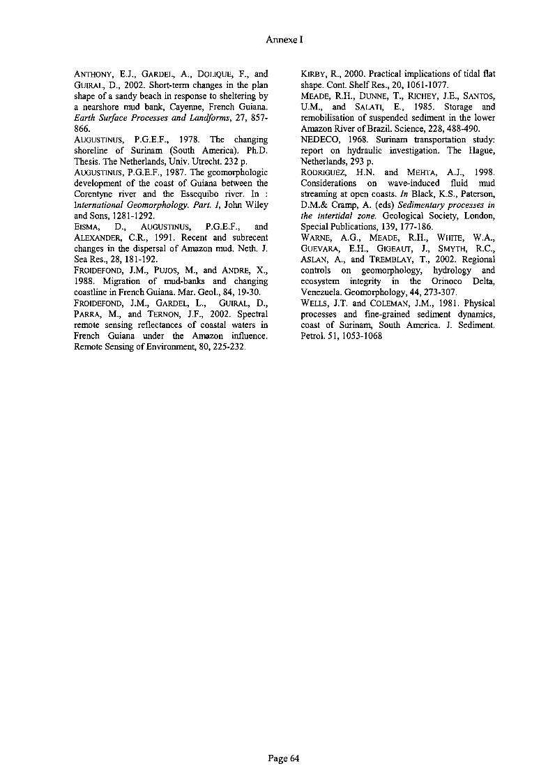
Annexe I
ANTHONY, EJ., GARDEL, A, DOLIQUE, F., andGUIRAL, D., 2002. Short-term changes in the planshape of a sandy beach in response to sheltering bya nearshore mud bank, Cayenne, French Guiana.Earth Surface Processes and Landforms, 27, 857866.AUGUSTINUS, P.G.E.F., 1978. The changingshoreline of Surinam (South America). Ph.D.Thesis. The Netherlands, Univ. Utrecht. 232 p.AUGUSTINUS, P.G.E.F., 1987. The geomorphologiedevelopment of the coast of Guiana between theCorentyne river and the Essequibo river. In :International Geomorphology. Part. l, John Wileyand Sons, 1281-1292.ElSMA, D., AUGUSTINUS, P.G.E.F., andALEXANDER, C.R., 1991. Recent and subrecentchanges in the dispersal of Amazon mud. Neth. J.Sea Res., 28,181-192.FROIDEFOND, J.M., PUJOs, M., and ANDRE, x.,1988. Migration of mud-banks and changingcoastline in French Guiana. Mar. GeoI., 84, 19-30.FROIDEFOND, J.M., GARDEL, L., GUIRAL, D.,PARRA, M., and TERNON, J.F., 2002. Spectralremote sensing reflectances of coastal waters inFrench Guiana under the Amazon influence.Remote Sensing of Environment, 80, 225-232.
Page 64
KIRBY, R., 2000. Practical implications of tidal flatshape. Cont. ShelfRes., 20,1061-1077.MEADE, R.H., DUNNE, T., RICHEY, J.E., SANTOS,U.M., and SALAT!, E., 1985. Storage andremobilisation of suspended sediment in the lowerAmazon River ofBraziI. Science, 228, 488-490.NEDECO, 1968. Surinam transportation study:report on hydraulic investigation. The Hague,Netherlands, 293 p.RODRlGUEZ, H.N. and MEHTA, A.J., 1998.Considerations on wave-induced fluid mudstreaming at open coasts. In Black, K.S., Paterson,D.M.& Cramp, A. (eds) Sedimentary processes inthe intertidal zone. Geological Society, London,Special Publications, 139, 177-186.WARNE, AG., MEADE, R.H., WHITE, W.A,GUEVARA, E.H., GIGEAUT, J., SMYTH, R.C.,ASLAN, A, and TREMBLAY, T., 2002. Regionalcontrols on geomorphology, hydrology andecosystem integrity in the Orinoco Delta,Venezuela. Geomorphology, 44, 273-307.WELLS, J.T. and COLEMAN, J.M., 1981. Physicalprocesses and fine-grained sediment dynamics,coast of Surinam, South America. J. Sediment.Petrol. 51, 1053-1068
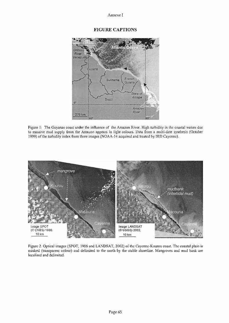
Annexe 1
FIGURE CAPTIONS
''':,,,,,,,,. . ' ,. ,,,·········\·1····00
1 :... --- - - -- - - - - ~- - - - - ----- - - -- ---- --- - - - -- - ..- - ...... - -- - - - _..... ~ _....... - - ---: ,: Amazon i: River :
2~km : :.... :60· :So'
Figure 1: The Guyanas coast under the influence of the Amazon River. High turbidity in the coastal waters dueto massive mud supply from the Amazon appears in light colours. Data from a multi-date synthesis (October1999) of the turbidity index from three images (NOAA-14 acquired and treated by IRD Cayenne).
Figure 2. Optical images (SPOT, 1986 and LANDSAT, 2002) of the Cayenne-Kourou coast. The coastal plain ismasked (transparent colour) and delimited to the north by the stable shoreline. Mangroves and mud bank arelocalised and delimited.
Page 65

Annexe l
5.8 x "
5.75
5.7
E5.65
~>- 5.6
5.55
5.5
....... shorellne- mangrove- Inlertldal
X xOz ortgln
3a3.1 3.15 3.2 3.25 3.3 3.35 3.4
x.rrN (m)
3.45
x 10'
5000I-~~-~--~--~---;==~:::=:::=il
•x 10
543x (m)
1000
O:l!======='~----==~__-,-----_-----l.~=:....d
o3b
4000
~ 3000&N 2000
6
x 10'
543
x(m)
ob==~====!'-'---__...L.ÇL-_'-----_~==",,"
o3c
4000
~ 2000
Figure 3. Steps in the standardisation of mangrove and inter-tidal mudflat limits, applied to the image acquired in07/02/01.
4000
3000
2000
1000
0
'j,610•
(m)
4000
3000
2000
1000
0(m)
)(10·
3x (m)
3x(m)
o4a
2000
19851'-----''---~----'~-~----'--~o
4b
1990
2005
1985
~1, 1995
2005
1990
2000=:~
1, 1995
Figure 4. Matrix representation of the standardized results (a), and interpolation by Delaunay cubic triangulation(b). The colour gradient represents the distance of the inter-tidal mud bank limits (in metres) to the fixedshoreline.
Page 66
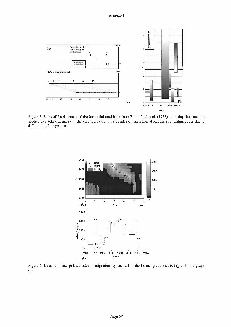
Annexe l
Resulte u'iingr..11 r:llil<:data
15
1979~bs
82
.,km
1991
Fro idcto ed <::1 al.res ult.. lDillF. aerialphotogrsphs S-I
....----.f----1
5a
112 111 on1U t
km H 12 JO
98 95
1
~;<----<--------_f---<--I'"
5b19:9 sz 8-l 91 95969800010,
Figure 5. Rates of displacement of the inter-tidal mud bank from Froidefond et al. (1988) and using their methodapplied to satellite images (a); the very high variability in rates of migration of leading and trailing edges due todifferent tidal ranges (b).
2000
4000
3000
1000
5 6 (m)
x10'
42
2000
1985 L-_---'---_~~_---'---_~~_ __'__~
a6a
1990
§: 1995N
2005
4000
1992 1994 1996 1998 2000 2002 2004years
1
111
i..
,-,1
1
1
1
t-~1
1
11
1
1 1L_ 1 1
1 11 1
,----::---:'--11
6b
3000
";'"::-:-
~ 2000.,a;u 1000
Figure 6. Direct and interpolated rates of migration represented in the lE-mangrove matrix (a), and on a graph(b).
Page 67

Annexe l
Photograph " elo ri ly Angle of waveda les km.y- incidence (NE)
19421950 10'
Guyana1962; 19t>-!
0.5 -2.5 "<1972/19751979 : 19801984
1947/19481957 45°
Suriname 1966 0.5 - 5 --L197019811955
French 197903-14 ~Guiana 1982 15'
198410-60 km long3-5 km wide low level
Morphological 5m tluckparamerers of the interbanc area 8-26 km longintertidal mudflat slopes :
between 1: 3000 to 1: 500(front part of banks)Tidal range (m): 0.6 -3.6Wave:
Relevant physical east \0 northeastparameters
height (m) 0.5-1.5period (s) 6-12
Figure 7. Dynamic and morphological characteristics of mud banks reported in the literature (NEDECO, 1968;Augustinus, 1978, 1987, Froidefond et al, 1988; Eisma et al. 1991; Allison et al., 2000; Anthony et al., 2002).
8a
8b
2
2
4
4
6 8months
6 8months
10
10
12
12
Figure 8. Average monthly wind velocities recorded in Kourou by Météo-France since 1975 (a), and from 1992to 2002 (b).
Page 68

•
Annexe 1
•
••
2km
Figure 9. Local morphological characteristics and channel access to the Kourou harbour superimposed on anextract of the Landsat ETM image (09/06/2002). Limit of the mudflat in 2000 (-), in 2002 (_), embayment eutin mangroves (••••) and bedrock headland (.). Pk represents distance to the harbour in km along the accesschannel.
Page 69

ANNEXE II
Gardel, A., Gratiot, N., 2004. Monitoring of coastal dynarnics in French Guiana from 16 yearsof SPOT images. Journal of Coastal Research Special Issue 39 (sous presse).
Page 70

Annexe II
ISSN 0749-0208BrazilICS 2004 (Proccedings)pg- pgSI391 Journal ofCoastal Research 1-----
Monitoring of coastal dynamics m French Guiana from 16 years of SPOT satelliteImages
A. Gardelj and N. GratiottjLaboratolre Régional de télédétectionUnité ESPACE, IRD Guyane,BP 165, Rte de Montabo, Cayenne97323, Guyane Francaise, [email protected]
tLaboratoire d'écologie littorale,Unité ELISA, IRD Guyane,BP 165, Rte de Montabo, Cayenne97323, Guyane Francaise, [email protected]
ABSTRACT
GARDEL, A. and GRATIOT, N., 2004. Monitoring of coastal dynamics in French Guiana From 16 SPOTsatellite images. Journal ofCoastal Rescarch, SI 39 (Proceedings of the 8th International Coastal Symposium), .Itajai, SC-Brazil, ISSN 0749-0208.
The Guianas coast, northwest of the mouth of the Amazon river, experiences a very strong supply of muddysediment that entails major coastal modifications at seasonalto annual timescales. Mud supply is predominantlyin the form of mud banks migrating alongshore From the Amazon to the Orinoco. In this paper, focus is placed onthe geomorphic change that has affected the 60 km stretch of coastline between Cayenne and Kourou (FrenchGuiana) from 1986 to 2002. The remote sensing analysis demonstrates an overall erosion of 60 km2 of sea-frontmangrove swamps. A new mud bank migrating towards Kourou since 1991 has led to a significant reduction inerosion and has even enabled the commencement of mangrove colonization. A spatio-temporal matrix applied toboth the vegetated and inter-tidal parts of the mud bank highlights the interplay between mud bank migration andmangrove colonization.
ADlTlüNAL INDEX WüRDS: mud bank, mangrove, cohesive sediment, remote sensing
INTRODUCTION
The Guianas coast from Amapà, in Brazil, to the Orinoco Riverdelta in Venezuela (Figure 1) is the longest muddy coast in theworld. The longshore sediment f1ux along this northeastern coastof South America is driven by the seasonal supply of mud fromthe Amazon river. The Amazon discharge has been estimated at1.2x109 tons.y' (Meade et al., 1985). Fifteen to twenty percent ofthe sediment supply migrates northwestward along the Guianascoast, half of this load (1-1.5 x 10⁸ tons.y" ) migrating in highlyturbid suspensions in the coastal waters, while the other half (1 x10⁸ tcns.y') migrates in the form of huge mud banks (Wells etColeman, 1978) whose formation occurs along the northwesterncoast of Amapà State in Brazil (Allison et al., 2000). The mudbanks then migrate along the French Guiana, Surinam and Guyanacoasts until the Orinoco delta in Venezuela (Warne et al., 2002).The mechanisms of this migration are complex, and are hinged onsediment supplY and hydrodynamic forcing. Migration is drivenessentially by trade wind-generated waves which allain their peakactivity between December and March (Wells et Coleman, 1978).The Guyana Current is deemed to be too far offshore to beeffective in the transport of coasta\ mud (Rodriguez and Mehta,1998).
The morphology of the mud banks appears to be variable. Theyrange in length from lOto 60 km, are 20 to 30 km wide, spaced 15to 25 km apart and are up to 5 m thick (Froidefond et al., 1988;Allison et al., 2000). Their rates of migration are also quitevariable, from less than 0.5 krn.y' to more than 5 krn.y'(Augustinus, 1987; Eisma et al., 1991 ; Froidefond et al., 1988). InFrench Guiana annual rates were estimated (Froidefond et al.1988) at about 1.0 krn.y" , A recent study by Gardel and Gratiot
(subrnitted) has recorded rates of migration twice higher (2.2km.y') during a J2-year survey of a mud bank using satellite data.This work also highlighted large variability in rates of migration(from 1 to 3 km.y").
> 52%
l
150 km
Figure 1. The Amazon-inf1uenced South American coast(adapted from Eisma et al., 1991). Dots along the coastrepresent positions of mud banks monitored between FrenchGuiana and Venezuela by Delft Hydraulics (1962).
Journal ofCoastal Research, Special Issue 39, 2004
Page 71

Annexe II
Gardel and Gratiot
Figure 2. photograph of a mature mangrove swarnp undergoingerosion (courtesy of M.T. Prost).
This paper focuses specifically on the French Guiana coast. Thecoastal morphology of French Guiana largely reflects theinfluence of mud supply From the Amazon river. The coastal plainhas a width of 10-30 km, and is backed inland by the BasementComplex formed by the Guyana Shield. From the shoreline to theGuyana Shield, the landscape is composed of a succession ofmorphological units. The young coastal plain, of Holocene age, issituated between an older, 10-20 km wide Pleistocene coastalplain that abuts the Shield, and the highly dynamic modem muddyshoreline. This humid coastal plain is interrupted in places bylinear relict Holocene beach ridges (old cheniers). The modemshore evolves permanently. Il can be muddy or sandy dependingon the presence or absence of a mud bank. Mud bank phases arecharacterised by large-scale development of mudflats andmangrove-colonized tidal flats. The colonization of mudflats bymangroves is not systematic. Il occurs following mudconsolidation driven by prolonged low-tide exposure of mud(Wells and Coleman, 1981) and by massive tidal deposition ofseeds. In the wake of such colonization, Avicennia germinansforrns exclusive sea-front stands, although Laguncularia racemosacommonly occurs in the initial phases of colonization. Inter-bankphases are dominated by erosion and commonly by the occurrenceof sandy (chenier or non-chenier) shores, as described From theSurinam coast by Augustinus (1979). Erosion can have aconsiderable impact, commonly engendering major morphologicalmodification of the coast. Large areas of mangroves can totallydisappear under wave action as shown in Figure 2.
The aim of this paper is ta apply a satellite image-basedmethod, recently developed by Gardel and Gratiot (submitted) tothe monitoring of geomorphic change along the 60-km stretch ofrnangrove-colonized coastline between the cities of Cayenne andKourou (Figure 1). Sixteen SPOT images and one LANDSATimage covering the period 1986 - 2002 are used to monitor theevolution of this part of the French Guiana coast. Ali the imageswere geo-coded and integrated in a GIS (Geographie InformationSystem) in order to extract mangrove limits at every date. Thisallowed a global analysis of the coastal dynamics and aquantification of mangrove erosion and new colonization. Amatrix representation of the relative evolution of mangroves since1986 highlights the direct interaction between mud bank evolutionand mangrove behaviour.
DATA AND METHüDS
High resolution satellite images such as SPOT and LANDSATare weil adapted to the monitoring of highly dynamic coastalfeatures such as those of the Guianas coast. Their multi-spectralresolution in the visible and infrared domains offers a good toolfor the identification of mangrove forests. At the observation scaleprovided by these satellite images, mangrove features arehomogeneous (due ta the monospecific and same-age character ofmangrove forests) and can thus be easily discriminated. The set ofdata contains sixteen SPOT images from 1986 to 2002 and aLANDSAT image acquired in September 2002 that completes andupdates the set. Ail images were geometrically processed andgeographically formatted in WGS84 UTM N22 projection. Theseinitial treatments were realized using ER Mapper (©) softwareversion 6.21 . The geo-coded images were then integrated in a GISsoftware (GeoConcept ©). The set of images, their dates ofacquisition, their coverage rates and the corresponding tidal levelsare reported in Table 1.
A manual method based on interpretation of satellite images hasbeen chosen to extract mangrove limits. The stable shoreline hasalso been extracted. The stable shoreline limit corresponds to thefirst Holocene sandy ridge. This structural Iimit is observed to bestable for the duration of the survey covered by the images. Atpresent, this Holocene sandy ridge is subjected to erosion in theinter-bank areas.
ln the GIS, the shoreline has been eut out in ten sectorsuniforrnly-spaced 4 km apart. The evolution of mangroves ismeasured in each sector and at every date. This step is effectedusing topological analysis between sectors and mangrove surfaces.
A matrix method was developed for the monitoring of mudbank migration (Gardel and Gratiot, submitted). This methodallows for a relevant spatio-temporal monitoring of inter-tidal mudbank limits, but also mangroves, and, more generally, theevolution of ail mathematical combinations of coastal features.
.Table 1. Sorne characteristics on the remote sensing imagesacquisition.
Date timeUTTidal Coverage
height (m) rate %10-20-86 14h16 1,28 10011-17-91 14h13 2,40 5010-02-93 13h56 1,14 5508-30-94 14h12 2,28 8510-16-95 13h49 2,35 9010-26-95 13h57 1,14 8009-28-96 13h55 0,86 9009-02-97 14h20 0,97 4506-20-98 13h57 2,11 4009-06-98 13h57 0,74 9005-09-99 13h45 2,65 4002-07-00 14h16 1,20 7007-02-01 13h49 1,58 10010-14-01 13h49 1,40 4012-14-01 14h16 1,28 7008-05-02 14h15 1,78 6009-19-02 12h30 1,05 100
Journal of Coastal Research, Special Issue 39, 2004
Page 72
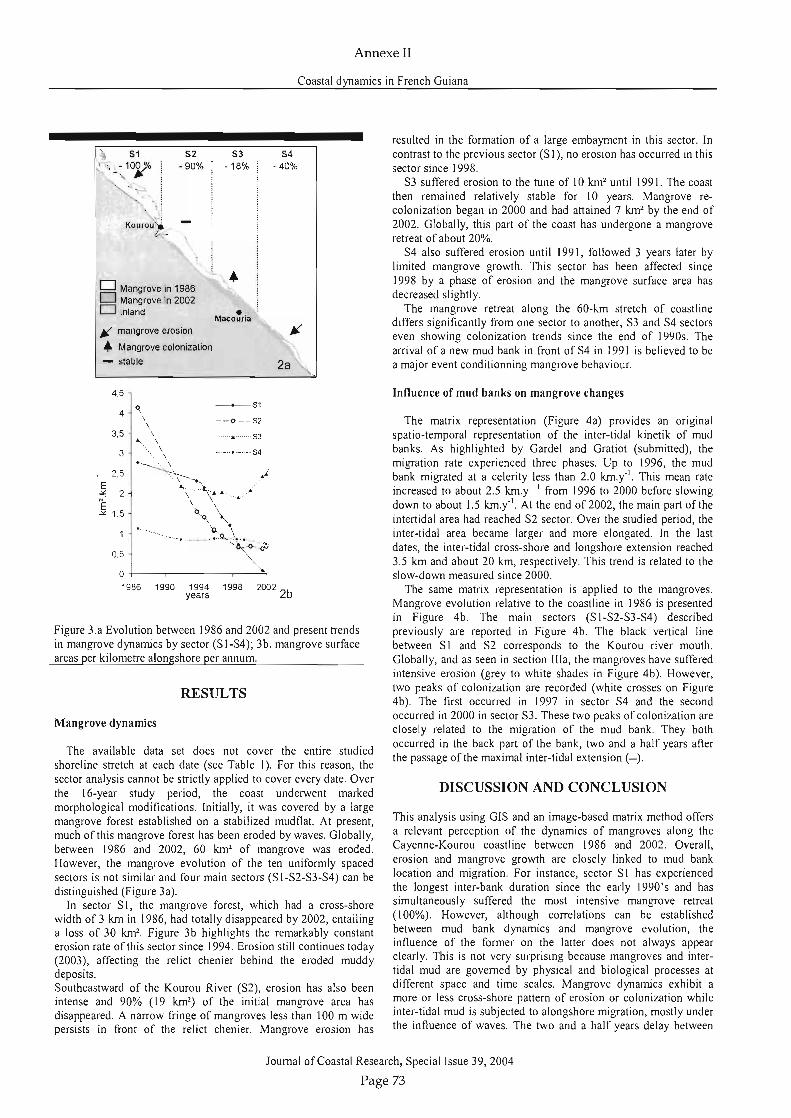
Annexe II
Coastal dynamics in French Guiana
S1 S2 S3 S4,·.,., - 1~ -90% -18% -40%
.-"',. ,.,.'Kourou".
/..- -
D Mangrove in 1986. ....
D Mangrove in 2002D Inland •Milcouri<J
Ji mangrove erosion Ji.... Mangrove colonizalion
- stable 2a,
4.5
Figure 3.a Evolution between 1986 and 2002 and present trendsin mangrove dynamics by sector (S I-S4); 3b. mangrove surfaceareas per kilometre alongshore per annum.
RESULTS
Mangrove dynamics
The available data set does not cover the entire studiedshoreline stretch at each date (see Table 1). For this reason, thesector analysis cannot be strictly applied to cover every date. Overthe 16-year study period, the coast underwent markedmorphological modifications. Initially, it was covered by a largemangrove forest established on a stabilized mudflat. At present,much of this mangrove forest has been eroded by waves. Globally,between 1986 and 2002, 60 km2 of mangrove was eroded.However, the mangrove evolution of the ten uniformJy spacedsectors is not similar and four main sectors (S I-S2-S3-S4) can bedistinguished (Figure 3a).
In sector SI, the mangrove forest, which had a cross-shorewidth of 3 km in 1986, had totally disappeared by 2002, entailinga loss of 30 km' . Figure 3b highlights the remarkably constanterosion rate of this sector since 1994. Erosion still continues today(2003), affecting the relict chenier behind the eroded muddydeposits,Southeastward of the Kourou River (S2), erosion has also beenintense and 90% (19 km') of the initial mangrove area hasdisappeared. A narrow fringe of mangroves less than 100 m widepersists in front of the relict chenier. Mangrove erosion has
resulted in the formation of a large embayment in this sector. Incontrast to the previous sector (S 1), no erosion has occurred in thissector since 1998.
S3 suffered erosion to the tune of 10 km2 until 1991. The coastthen remaincd relatively stable for 10 years. Mangrove recolonization began in 2000 and had attained 7 km2 by the end of2002. Globally, this part of the coast has undcrgone a mangroveretreat of about 20%.
S4 a1so suffered erosion until 1991, followed 3 years later bylimited mangrove growth. This sector has been affected since1998 by a phase of erosion and the mangrove surface area hasdecreased slightly.
The mangrove retreat along the 60-km stretch of coastlinediffers significantly from one sector to another, S3 and S4 sectorseven showing colonization trends since the end of 1990s. Thearrivai of a new mud bank in front of S4 in 1991 is believed to bea major event conditionning mangrove behaviour.
Influence of mud banks on mangrove changes
The matrix representation (Figure 4a) provides an originalspatio-temporal representation of the inter-tidal kinetik of mudbanks. As highlighted by Gardel and Gratiot (submitted), themigration rate experienced three phases. Up to 1996, the mudbank migrated at a celerity Jess than 2.0 km.y". This mean rateincreased to about 2.5 km.y-l from 1996 to 2000 before slowingdown to about 1.5 krn.y'. At the end of 2002, the main part of theintertidal area had reached S2 sector. Over the studied period, theinter-tidal area became larger and more elongated. In the lastdates, the inter-tidal cross-shore and longshore extension reached3.5 km and about 20 km, respectively. This trend is related to theslow-down measured since 2000.
The same matrix representation is applied to the mangroves.Mangrove evolution relative to the coastline in 1986 is presentedin Figure 4b. The main sectors (S I-S2-S3-S4) describedpreviously are reported in Figure 4b. The black vertical linebetween SI and S2 corresponds to the Kourou river mouth.Globally, and as seen in section IIIa, the mangroves have sufferedintensive erosion (grey to white shades in Figure 4b). However,two peaks of colonization are recorded (white crosses on Figure4b). The first occurred in 1997 in sector S4 and the secondoccurred in 2000 in sector S3. These two pcaks of colonization areclosely related to the migration of the mud bank. They bothoccurred in the back part of the bank, two and a half years afterthe passage of the maximal inter-tidal extension (-).
DISCUSSION AND CONCLUSION
This analysis using GIS and an image-based matrix method offersa relevant perception of the dynamics of mangroves along theCayenne-Kourou coastline between 1986 and 2002. Overall,erosion and mangrove growth are closely linked to mud banklocation and migration. For instance, sector SI has experiencedthe longest inter-bank duration since the early 1990's and hassimultaneously suffered the most intensive mangrove retreat(100%). However, although correlations can be establishedbetween mud bank dynamics and mangrove evolution, theinfluence of the former on the latter does not always appearclearly. This is not very surprising because mangroves and intertidal mud are governed by physical and biological processes atdifferent space and time scales. Mangrove dynamics exhibit amore or Icss cross-shore pattern of erosion or colonization whileinter-tidal mud is subjected to alongshore migration, mostly underthe influence of waves. The two and a half years delay between
Journal ofCoastal Research, Special Issue 39,2004
Page 73

Annexe II
Gardel and Gratiot
Figure 4a. matrix representation of the inter-tidal mud bankevolution (1986-2002) and evolution of the maximal inter-tidalextension (-). 4b. matrix representation of the relativeevolution of mangroves since 1986. White crosses representcolonization spots. 4c. temporal evolution of mangroves,discriminating bank and inter-bank areas on Figure 4a.
":>.
Ê -0.2ir=====;-~-~/\--"li -0.1 1-=- ~~~~bank I~rv~"0 00 EROSION \ /\, . (~ . COLONISATION \ . r : :CD J \ 1
~ 0.1 V0>
~ 1980 1985 1990 1995 2000
LITERATURE CITED
ACKNOWLEDGEMENTS
This work was supported by CNESIIRD contractn002/CNES/0814/00. PNEC (Programme Nationald'Environnement Côtier) provided sorne of the SPOT images. Wewish to thank Météo France for the wind data and Edward lAnthony for the fruitful discussions and his review of themanuscript.
on a more global forcing context and on the duality between theinter-bank areas (black areas in Figure 4a) in erosion (see Figure4b) and bank areas that are the potential zones of mangrovecolonization.
Future research should focus on reasons for the variability ofmud bank migration rates and its incidence on mangrovedynamics. Low-frequency tidal constituents are very likely to be adeterminant factor in the consolidation process (Wells andColeman, 1981 ) while wind stress (intensity and direction)variations at local and synoptic scales may significantly modifywave forcing.
ALLiSON, M.A.; LEE, M.T.; OGSTON, A.S.; and ALLER, R.C., 2000.Origin of Amazon mudbanks along he northeastern coast of SouthAmerica. Marine Geology, 163,24 1-256.ANTHONY, E.J.; GARDEL, A.; DOLIQUE, F.; and GUIRAL, 0 ., 2002.Short-lerm changes in the plan shape of a sandy beach in responseto sheltering by a nearshore mud bank, Cayenne, French Guiana.Earth SU/face Processes and Landform s, 27, 857-866.AUG USTINUS, P.G.E.F., 1978. The changing shoreline of Surinam(South America). The Netherlands, University of Utrecht, Ph.D.thesis, 232p.AUGUSTl1\TUS, P.G.E.F., 1987. The geomorphologie developmentof the coast of Guiana between the Corentyne river and theEssequibo river. In: John Wiley and Sons (ed.): InternationalGeomorphology. Pari. 1, pp.1 281-1292.BOYE, M., 1962. Les palétuviers du littoral de la Guyanefrançaise, ressources et problèmes d'exploitation. Les Cahiersd'Duire -mer, 15,271-2 90.DELFT HYDRAULICS LABORATORY, J962. Dernerara coastalinvestigation. Report on siltation of Demerara Bar Channel andcoastal erosion in British Guiana. Delft, 1-240.EISMA, O.; AUGUSTINUS, P.G.E.F., and ALEXANDER, C.R., 1991.Recent and subrecent changes in the dispersal of Amazon mud.Netherland Journal ofSea Research, 28, 181-192.FROIDEFONO, l M.; PUJOS, M.; and ANDRE, X., 1988. Migration ofmud-banks and changing coastline in French Guiana. MarineGeology, 84, 19-30.FROIDEFOND, lM. ; GARDEL, L.; GUI RAL, O.; PARRA, M., andTERNON, lF., 2002. Spectral remote sensing reflectances ofcoastal waters in French Guiana under the Amazon influence.Remote Sensing ofEnvironment , 80, 225-232.GARDEL, A.; and GRATIOT, N. A satellite image-based method forestimating rates of mud banks migration, French guiana, SouthAmerica. Journal ofCoastal Research, submitted.KIRBY, R., 2000. Practical implications of tidal flat shape.Continental ShelfResearch., 20, 1061-1077.MEADE, R.H.; DUNNE, T.; RICHEY, J.E.; SANTOS, U.M.; andSALATI, E., 1985. Storage and remobilisation of suspendedsediment in the lower Amazon River of Brazil. Science, 228, 488490.NEDECO, J968. Surinam transportation study: report onhydraulic investigation. The Hague, Netherlands, 293 p.
2 .0
3.0
2.5
2.0
1.5
1.0
0.5
okm
05
00
CIl
ro 95<Il>-
90
850 2 4 6
05 r SI S2 S3 S4
00
CIl
ro 95<Il>-
90
850 2 4 6
the passage of the maximal inter-tidal extension and the beginningof colonization (see Figure 4b) highlights the complex and longterm interplay between mud bank and mangroves. The increase ofthe cross shore inter-tidal mud extension first protects the coastfrom waves, allowing for the onset of soil consolidation processes.The transport of seeds by tidal currents or creeks and their arrivaIat low-tide exposure of the mudflats is then a critical condition forthe deposition of seeds and the initiation of colonization.
The relationship between inter-tidal mud bank and mangroves ismore evident when inter-bank and bank areas are examinedindependently. Results presented in Figure 4c demonstrate theexistence of three distinct periods. From 1986 to 1995, vegetationsuffered erosion in both inter-bank and bank areas; the following1995-2001 period was very active for both erosion process ininter-bank areas and colonization in bank areas ; finally, mangrovecolonization ceased in 200 1 while erosion rates rose back to ahundred m.y' in inter-bank areas. The dilTerent phases are weilcorrelated with the variability of mud bank migration ratesquantified by Gardel and Gratiot (submitted). This demonstrates ahigh time dependency of both mud bank and mangrove dynamics
Journal of Coastal Research, Special Issue 39, 2004
Page 74

Annexe II
Coasta1 dynamicsin French Guiana
RODRIGUEZ, H.N. and MEHTA, AJ., 1998. Considerations onwave-induced fluid mud streamingat open coasts. In BLACK, K.S.;PATERSON, D.M., and CRAMP, A. (eds.) Sedimentary processes inthe intertidal zone. Geological Society, London, SpecialPublications, 139, 177-186.WARNE, AG.; MEADE, R.H.; WHITE, W.A; GUEVARA, E.H.;GIGEAUT, J.; SMYTH, R.C.; ASLAN, A, and TREMBLAY, T., 2002.Regional controls on geomorphology, hydrology and ecosystem
integrity in the Orinoco Delta, Venezuela. Geomorphology, 44,273-307.WELLS, J.T. and COLEMAN, J.M., 1978. Longshore transport ofmud by waves: northeastern coast of South America. Geologie enMijnbouw. 57, 353-359.WELLS, J.T. and COLEMAN, J.M., 1981. Periodic mudflatprogradation, northeastern coast of South America: a hypothesis.Journal ofSediment Petrology. 51,1069-1075.
Journal ofCoastal Research, Special Issue 39, 2004
Page 75

Annexe III
ANNEXE III
GRATIOT, N., GARDEL, A. & ANTHONY, E. Atlantic trade-wind waves and mud bankdynamics in French Guyana: a temporal perspective. Marine Geology (soumis).
Page 76

Annexe III
Atlantic trade-wind waves and mud bank dynamics on the French Guiana
coast, South America
Nicolas Gratiot", Antoine Gardel", Edward, J. Anthony"
"Laboratoire d'Ecologie Littorale, (UR053 Elisa) IRD, BP 165, Rte de Montabo, 97323 Cayenne, French GuianabLaboratoire Régional de Télédétection (US140 Espace), IRD Guyane, BP 165, Rte de Montabo, 97323Cayenne, French GuianaC Coastal Geomorphology and Shoreline Management Unit (GéoDAL), EA 3599, Université du Littoral Côted'Opale, MREI 2, 189a Avenue Maurice Schumann, 59140 Dunkerque, France
AbstractWind pseudo-stress data from the tropical Atlantic have been used as a surrogate to
determine temporal fluctuations in trade-wind generated wave activity affecting the coast ofFrench Guiana. Fluctuations of the wind field at a multi-annual time scale show that suchoceanic waves are a major factor in the mobilisation and migration of the Amazon-derivedmud banks that periodically affect this coast. The mud banks are composed of underconsolidated (~1350kg.m-3) mud subjected to marked rheological changes under wave action.Virtually total attenuation of swell occurs in the peripheral outer zone of the mud banks, thusresulting in zero energy over the large inter-tidal mudflats formed by these banks. Mud bankmigration involves mud liquefaction by waves and mass streaming alongshore to thenorthwest because of the obliquely incidence of incoming waves. This liquefied mud lead tothe formation of bar-like features that have been described in the literature. Waves generatedlocally do not seem to play a significant role in mud bank migration. However, they could beof importance in inshore mangrove erosion processes. Fine quantitative prediction of mudbank migration rates is limited by three factors: (1) the use of the available monthly averagedwind data set whose temporal resolution is not fine enough, and which thus tend to smoothout rates, (2) the potential variability of mud bank rheological properties, which depend notonly on the effects of wave forcing, but also on factors such as dewatering and mangrovecolonisation, (3) antecedent large-scale variations in coastal morphology and smaller-scalecoastal irregularities such as bedrock outcrops, headlands and river mouths, all of whichinfluence mud transport alongshore.
Keywords: Mud banks, mangroves, wind-wave generation, fetch, French Guiana.
1. IntroductionThe Guianas coast (Fig. 1), extending over 1600 kilometres between the mouths of the
Amazon and the Orinoco rivers, is bounded by the longest stretch of muddy shoreline in theworld. This coast comprises mangrove-colonised tidal flats and bare mudflats severalhundreds of metres to several kilometres wide. These deposits have been supplied from themuddy sediments supplied by the Amazon and transported northwestwards towards theOrinoco Delta (Augustinus, 1978; Eisma et al., 1991). Fifteen to twenty percent of theAmazon sediment supply (:::l.2 109 tonnes.y") is transported in highly turbid suspensions(:::l06 tonnes.y"), but also in distinct mud banks (:::l.0-1.5 106 tonnes.y") that weld onto theshore in places (Wells and Coleman, 1981; Meade et al., 1985; Eisma et al., 1991; Warne et
Page 77

Annexe III
al., 2000). Individual mud banks are about 10-60 km long, 10-15 km wide and 1-3 m thick(Augustinus, 1978; Wells and Coleman, 1981; Froidefond et al., 1988; Eisma et al., 1991;Rodriguez and Mehta, 1998; Allison et al., 1995, 2000). At any given stretch of shoreline,individual mud banks migrating alongshore are separated by inter-bank phases. Thisrhythmicity of bank and inter-bank phases has an overwhelming impact on coastal activitiesand management as it is attended directly and indirectly by strong and rapid shorelineaccretion and/or erosion involving frequent and large-scale mangrove colonization anddestruction. For instance, the arrival of a mud bank can create an intertidal mudflat of severalsquare kilometres in a few months, followed by very dense mangrove development in a fewyears. Mud banks migrating alongshore affect recreational activities along the coast, access toestuary mouths and ports, and the ecological dynamics of the coastal zone.
Fig. 1.
In the last three decades, there have been attempts to identify the hydrodynamic forcinggoveming the formation ofmud banks and their migration, and various experimental and fieldinvestigations have pointed out the leading role of wind-generated waves in these processes(e.g., Augustinus, 1978; Wells and Coleman, 1978; Eisma et al., 1991; Jiang and Mehta,1996; Rodriguez and Mehta, 1998). However, there is still a need to clarify and quantify theinterplay between the hydrodynamic forcing, mud banks and the coastal morphology. Apartfrom the lack of appropriate and reliable local data on winds and waves, one major difficultyresides in the heterogeneity of the shape of the coast, which involves various irregularitiessuch as bedrock headlands, river mouths, and offshore bedrock isles, and the rapidity ofchanges related to bank and inter-bank relationships with the coast (e.g., Anthony et al.,2002). Gardel and Gratiot (in press a) showed that this problem may be partially resolved byusing modem remote sensing data. This technique provides information on coastline changesat high temporal and spatial resolutions. It is surprising that it has not been used more widelyto study the nearshore sediment dynamics of the Guianas.
The spacing between the banks may reflect seasonal to multi-annual variations in theAmazon mud supply system and temporal variability in migration rates hinged on theintensity of the trade winds (Eisma et al., 1991; Allison et al., 1995, 2000), which determinewave activity off this coast. The waves on the French Guiana coast arrive from an east tonortheast direction in response to the prevailing trade winds. They have typical periods of 6 to12 sec, and offshore heights ofup to 1.5 m. The most energetic waves are observed during therainy season, especially between December and March when the trade winds peak. The tidesare semi-diumal and the tidal range is low-mesotidal with a spring range of 2.9 m and a neaprange of 0.8 m in Cayenne.
The lack of long-term records ofwaves on the French Guiana coast necessitates recourse toproxy data on wave-generating winds. Conceptually, one may consider that the interplaybetween wind and coastal dynamics is a two-step operation. First, local and synoptic windsstress the ocean surface and generate gravity waves. Then, the waves propagate shorewardand transfer their energy to the coastal area through breaking or dissipative dampening. Thephysical process through which energy is transferred from wind to waves is satisfactorilydescribed in literature. The basics of this process are briefly introduced in section 3 beforefocusing on the statistical description of both the local and synoptic wind fields, withparticular attention to fluctuations at seasonal and multi-annual timescales. The processesinvolved in the transfer of energy from waves to the shore are much more complex. However,their overall impact can be schematically depicted as proposed in section 4. Finally, theaforementioned wind forcing and its variations will be discussed with regard to previousresults on the dynamics of mud banks and mangroves (Froidefond et al., 1988; Gardel and
Page 78
Annexe III
Gratiot, in press a, in press b). This comparison brings out interesting information on thenature of the interplay between winds and the coast of French Guiana, and highlights thelimitations of attempts at finely predicting mud bank migration rates.
2. Data acquisitionLocated between 4 and 6° north latitude, French Guiana experiences a tropical climate, and
is directly under the influence of trade winds. Two types of wind data have been used in thisstudy. Local wind data on the coast of Guiana are derived from the weather station of Devil'sIslands (5.28°N, 52.58°E) located 20 km off-shore. Météo-France has acquired data onmonthly-averaged mean wind intensity and mean wind direction since 1975 and a semihourly data set since 1991. The latter data are acquired automatically at an elevation of 10metres above sea level. The data acquired prior to 1991 are rather scarce and somewhatquestionable because they were acquired by successive individual operators. The second typeof data is derived from the !RD tropical Atlantic pseudo-stress data base and is used todetermine the Atlantic oceanic wind field and its influence on wave activity on the coast ofFrench Guiana. This database is currently available on the URL pagewww.coaps.fsu.edu/woce/SAC/atlantic. The pseudo-stress maps coyer the tropical Atlantic(300N-300S, 1200E-700W) with a 2°x2° spatial resolution at a monthly-averaged temporalresolution since 1961. As reported in the URL page, all data set matrices are derived fromindividual observations that were screened, binned and subjectively analyzed.
Nearshore profiles of typical inter-bank and mud bank regions were measured by echosounding in November 2002. The profiles are located about twenty kilometres apart. The GPShorizontal positioning accuracy is about ±10 m and the water depth measurement precision isabout ±0.5 m. Sorne bed sediment sampling was realised simultaneously in order to examinethe sediment density along the water depth profiles. Their resolution is of about ±5%.
3. Waves generated by local and oceanic wind fields
The generation of waves by wind is initiated by randomly distributed pressure fluctuationsat the water-air interface and is followed by non linear wind-wave and wave-waveinteractions. These interactions transfer energy from high to low frequencies causing the wavespectrum to change with time as described by Hasselmann et al. (1973). For a fully developedsea, i.e., when considering that the wind blows with a constant speed U over a fetch of1engthX for a sufficient time, the wave period and the wave height will increase with U and Xfollowing Hasse1mann et al. (1973):
(La)
(Lb)
where Ho is the significant wave height (m), Tp the peak frequency of the JONSWAP wavespectrum (s), X the distance over which the wind blows with a constant speed and direction(m), g the gravitational acceleration (m.s"), U the wind speed measured 10 meters above thesea surface (m.s"), Cl and C2 constants derived from the wave data collected during theJONSWAP campaign (Hasse1mann et al., 1973), respective1y 1.6x10⁻³ and 285.3x10⁻³
.
Page 79

Annexe III
Equations la and lb indicate that the increase in wave height is principally govemed bywind velocity while the wave period is affected by wind velocity as much as by fetch length.The hypothesis of a fully developed sea state is usually satisfied for waves generated over alocal fetch, so that equations la and lb are usually valid. For large oceanic fetches, the timeduring which the wind blows can become a limiting factor and has to be examined. The windhas to blow for a sufficiently long time to stress the waves during their propagation along thefetch length.
The !RD tropical Atlantic pseudo-stress data used are matrices of 25 lines and 38 rows. 473monthly-averaged matrices covering the (300N-300S, 1200E-700W) geographie position wereused to obtain the mean Eulerian directions and intensities and their corresponding standarddeviations. Results of the calculation are reported in Fig. 2. The trade winds affecting theFrench Guiana coast are characterized by a quasi-constant direction throughout the year.When examining the standard deviation of the monthly-averaged pseudo-stress wind directionfrom 1964 to 2003 (Fig. 2b), the trade wind regions are clearly delimited. They correspond tothe dark areas, associated with a small standard deviation (0-10°). In these areas, winds blowalmost permanently in the same direction but also with a rather strong intensity as can be seenin Fig. 2c. Thus, the monthly-averaged pseudo-stress wind values reach maximum intensitiesof about 60 m2.s-2 in the 10-200N trade wind region. As illustrated in Fig. 2d, wind velocityfluctuations can be important, especially offshore of French Guiana (indicated by a 'star')where the standard deviation can reach 25 m2.s-2
• In fact, it corresponds to monthlyfluctuations, so that the standard deviation is considerably reduced when considering interannual variability. This point will be evoked later.
Fig. 2.
To determine the influence of the oceanic wind field on wave activity along the coast ofFrench Guiana, it is necessary to determine first the associated fetch area. The establishmentof the fetch area cannot be done strictly from the available monthly-averaged wind field data.It is therefore more appropriate to consider a monthly averaged pseudo-fetch area. From the456 monthly-averaged wind pseudo-stress direction matrices available, it is possible toestablish a month-to-month pseudo-fetch area, but for simplicity it has been decided toconsider a time-independent area. This latter is represented by small circles in Fig. 1a. Thischoice of a geographically constant pseudo-fetch area is physically suitable because it fitswith the location of the trade wind region so that wind direction can be considered as almostconstant. This choice simplifies the month-to-month matrix comparisons because the areaconsidered is constant. The pseudo-fetch area thus determined covers N=48 points of eachmatrix with line and row coordinates regrouped in the 48 elements vectors ifandJf.
The mean wind velocity VI in the pseudo-fetch area is then calculated from the month-tomonth pseudo-stress wind velocity matrices using the following equations:
UxŒf,Jf])= T)[if,JfD 114
(('x([If,j(]))'{y{[tfJf]))'Ju (r:J" if]L 1y([if,jjn
y l1J ,1 F 2 2 1/4
((1x([if, jfn) +(1i[if,jj])) )
Vt=kÎ ~ViJj{i),jj{i))+Vi.jj{i),jj{i))i=1
Page 8D
(2.a)
(2.b)
(2.c)

Annexe III
where 'x and ry are the two horizontal components of the pseudo-stress wind field matrices,and U, and U; the two horizontal components of the wind field velocity in the pseudo-fetcharea.
Equations 2a, 2b and 2c do not provide an accurate estimate of the wind velocity, becausethe root square of the monthly averaged pseudo-stress data deviates mathematically from themonthly averaged root square pseudo-stress. For this reason, the time evolution of the meanwind velocity Ufin the pseudo-fetch area shown in Fig. 3 is discussed qualitatively and notquantitatively.
There is a significant seasonal variation, and it is much larger than inter-annual fluctuations.The strongest winds occur from January to May with velocities one and half times higher thanthose measured during the weak wind season from July to October. The seasonality in thepseudo-fetch area is well established as it is observed on a multi-decennial time scale since1964. It also seems to concern the coastal fringe, as Eisma et al. (1991) deduced a strongJanuary-April wind season from measurements recorded at an elevation of 500 m elevation inKourou (French Guiana) from 1953 to 1986. The decennial trends show a measurableincrease of the annually averaged wind speed, from about 6.5-7.0 m.s-I in the late 1960s toabout 7.5 m.s" since the early 1990s. The fluctuations are much more pronounced for thestrong wind season (January-May) which is characterized by two multi-annual weak periodsfrom 1964 to 1970 and from 1978 to 1983.
Fig. 3.
The wind field patterns observed at the synoptic scale and presented in Fig. 3 are coupledwith local wind field observations. Semi-hourly wind measurements since 1994, as well as theweekly averaged wind field, are reported in Fig. 4a. The weekly averaged data (dots) areconcentrated within a sharp window centered on the East sector with wind speeds in the range[0-6 m.s"]. This unidirectional distribution is characteristic of the trade wind influence. Thesemi-hourly data are much more dispersed and coyer every sector. This pattern is due to dailyfluctuations caused by the land and sea breezes that regularly affect the coast of FrenchGuiana. However, it may be noted that this data dispersion disappears when semi-hourly windspeeds higher than 6 m.s" are considered. As reported in Fig. 4b, significant wind fieldvariations occur at a seasonal timescale. Slight variations of the wind field directionassociated with important variations of the wind speed can be noticed. The strong JanuaryMay winds blow from the E-SE sectors and the weak July-October winds from the E-NEsectors. The evolution of the wind field at the multi-annual scale is characterized by adecrease of wind velocity from 1974 to 1994 and rather constant values since. The annuallyaveraged wind speed was about 6.5 m.s" in the late 1970s and about 3.5 m.s" since 2000.However, it may be noted that the automatic station located on the coast in Kourou does notexhibit such a decrease. At this station, data have an almost constant annually-averaged windspeed that decreases slightly from about 3.6 m.s" in the late 1970s to about 3.4 m.s" in theearly 2000s.
Fig. 4.
The synoptic and local winds, presented in Fig.s 3 and 4, show significantly contrastingtrends over the last decades. The oceanic wind field shows a multi-decennial wind intensityincrease with strong seasonal and multi-annual fluctuations while the coastal data show adecrease until 1995, followed by stability since. These wind field trends undoubtedly
Page 81
Annexe III
modified wave activity along the coast of French Guiana with consequences on the coastaldynamics. These consequences cannot be considered globally and it is necessary to identifythe coastal dynamics in mud bank and inter-bank areas independently. This, because theinteraction of progressive waves with the sea bed is very sensitive to the water depth profileand to the rheological properties of the sediment (e.g., Wells and Coleman, 1981; Mathew etal., 1995; Jiang and Mehta, 1996).
4. Wave propagation over mud bank and inter-bank areas
In shallow-water areas, shoaling tends to increase the height of incoming waves to maintainthe flux of energy transported shoreward, while the increasing nearbed horizontal and verticalpressure gradients enhance the transfer and dissipation of energy within the bottom. Waveattenuation also depends on wave frequency so that observations and measurements remainessential for the comprehension of in situ wave-seabed interactions.
The nearshore profiles of the typical inter-bank and mud bank areas acquired by echosounding, and the sediment density along the water depth profiles are presented in Fig. 5.
Fig. 5.
The inter-bank profile (Fig. 5a) shows an almost 111000 linear slope (or slightly convexshape) from -15 m to 0 m and a pronounced concave profile above. The corresponding bedsediment (Fig. 5c) has a mud density of about 1450 kg.rn" over the whole profile. It istypical of an over-consolidated relict mud relict that was presumably formed during theHolocene. Allison et al. (2000) have shown that the mud banks migrate over a relict shelfmud surface in shallow inshore water depths of 5 to 20 m. The French Guiana inner shelfbetween 0 and -20 m shows thick deposits of mud from the Amazon (Bouysse et al.,1977) that range in age from over 40 ky to present (Cleac'h, 1999). The most superficialdeposits have been radiocarbon-dated as Holocene, and progressively accumulated as thePost-Glacial sea level rose (Pujos et al., 1990; Cleac 'h, 1999).
The mud bank profile presented in Fig. 5b is rather different. It shows a convex profile andis characterized by a mean bottom layer density of about 1350 kg.rn". At 6 to 7 km offshore,the mud bank profile presents a bar-like feature that is similar to those reported by Allison etal. (1995) and Jiang and Mehta (1996) from field measurement and laboratory experiments.The comparison of the inter-bank and mud bank profiles yields a mud bank thickness of about1-3 m and a cross-shore extension of about 10-15 km. These characteristics are consistentwith those reported in literature (Allison et al., 2000) and it may thus be considered that theinter-bank profile is somehow representative of the relict mud profile under the active mudbank. Details of the bottom sediment density are presented in Fig. 5d. The under-consolidatedbottom layer extends 13-15 km offshore. Beyond, the mud density increases to a value ofabout 1450 kg.rn", indicative of the relict mud. A high sediment density is also observed onthe shore as a result of dewatering and evaporation in the inter-tidal zone during exposure atlow tide.
High-resolution SPOT satellite scenes such as the one presented in Fig. 6 are particular1yuseful in identifying miscellaneous coasta1 features such as mangrove forests (black),intertidal mud bank areas and propagating and spilling waves. Among the whole set ofavailable images (Gardel and Gratiot, in press b), the scene depicted in Fig. 6 is particularlyillustrative of high swell conditions. In 16 m water depth, the estimated wavelength is about200 m and decreases to 150 m in 6-7 m water depths. From these wave parameters, theapplication of the Airy relation gives a wave period of about 17 s. This value is much greater
Page 82

Annexe III
than the 6-12 s wave period usually observed along the Guianas coasts (NEDECO, 1968;Anthony et al., 2002). However, the event captured by this satellite image is not unique and15 s wave periods were also measured a few months later by a wave recorder deployed on abeach in Cayenne (Fig. 1) during an inter-bank phase (Dolique, pers. corn., 2004). Althoughthey are not observed frequently, high swells are undoubtedly responsible for the mostsignificant geomorphic changes and consequently have to be considered with priority whendefining water-wave interaction.
Fig. 6.
In situ observations, aerial photographs and satellite images together enable a schematicdescription of wave attenuation in shallow water depths. This is reported in Fig. 5a and 5b.Over inter-bank areas, the swell propagates without breaking up to 3 m water depth (6-8 kmoff-shore). For shallowest water condition, waves break by spilling over the gentle 1/1000slope and are complete1y dampened near the shore. In mud banks areas, waves do not deviatesignificantly from the 2nd order Stokes theory up to about 5 m water depth (11-13 km offshore) and are totally dampened beyond a water depth of 1 m (6-8 km offshore). For thelowest wave conditions, solitary waves are frequently observed shoreward but this is not thecase in the image presented in Fig. 6.
Mud bank and inter-bank profiles demonstrate a wave-seabed interaction that agrees withthe conceptual muddy shore profiles proposed by Kirby (2000). Inter-bank area arecharacterized by receding low and concave erosion-dominated profiles of over-consolidatedmud while mud banks are characterized by prograding high and convex accretion-dominatedprofiles of soft mud. Depending on the tidal leve1 and on swell characteristics, it may beconc1uded that the main zone of interaction between waves and mud bank areas occurs inshallow water depths when kh is lower than 0.3, k being the wavelength and h the waterdepth. When this condition is met, almost all of the wave energy is transferred to the soft mudbed and the wave energy spectrum is drastically reduced. The interpretation of thepropagating waves over the mud bank profile presented in Fig. 4b is in a good agreement withthe physically suitable scenario proposed by Jiang and Mehta (1996) for wave-bankinteraction. Because of thixotropic conditions, the cyc1ic pressure gradients at the mud banksurface liquefy the mud which is then transported en masse by wave drift. This process hasbeen observed on beaches in Cayenne subject to liquefaction of intertidal mud during theonset of an inter-bank phase (Anthony and Dolique, accepted). For the shallowest waterdepth, the entire wave energy is dissipated and the sediment remains in situ. With cessation ofwave forcing, a fluid gel-like mud is rebuilt enabling the sediment to accumulate in the formofmud bars.
5. Influence of the trade-wind wave field on coastal geomorphology
The overall effect of wind-generated waves on the coast of French Guiana is based on aremote sensing survey of a 60 km stretch of linear coastline from the Cayenne River to fifteenkm eastward of the Kourou River. Gardel and Gratiot (in press a, in press b) and Froidefond etal. (1988) have shown that over the last fifty years, this coastline experienced the passage oftwo major mud banks separated by an active inter-bank period, from the middle 1980s to theearly 1990s. As shown in Fig. 7a, the maximum mangrove retreat during the inter-bank periodwas observed in the late 1980s. Retreat of the mangrove front was as high as 100 rn.y" ininter-bank areas and slightly less in front of mud bank areas. This corresponds to a mangroveloss of about 30 km2 from 1986 to 1991 along the 60 km shoreline. The mud bank migration
Page 83

(3)
Annexe III
rates are presented in Fig. 7b. The shoreline experienced consecutive phases of 10w and highmigration rates. Mud banks exhibit relatively low multi-annually averaged migration rates(1.5-2.0 km.y") in the 1960s, very high rates (3.5-4.5 km.y") in the 1970s, very low rates(0.2-1.8 km.y") in the early 1980s and high rates (1.8-3.0 km.y") over the last fifteen years.Overall, the migration rates are much higher than the usually quoted rates of 0.9-1.2 km.y"rates for the coast of French Guiana (Froidefond et al., 1988). Actually, this is not surprisingas the short term approach adopted by these workers and based on aerial photographinterpretation, coincided with a period of especially low migration rates.
Fig. 7
To assess the effect of local and synoptic wind fluctuations, and hence wave fluctuations, onmud bank migration rate, the parameterization proposed by Rodriguez and Mehta (1998) wasused. Their analytical mode! characterizes fluid mud streaming under non-breaking waveshear stress and is expressed by:
C -1' (fJwHnf h~p~ 2-p~ • 81J~bank- 3sma jJmT2 Jl h~ ~-1 1Jm 8;
h:p: 2-p: h: :-1 p:h~:h' '-1w m. .}• àrlw • •• • • àrlwXllm-'-[(hm+hwPm-hw]l1m- .as as
where a is the angle between the direction of wave propagation and the shoreline, Pw is seawater density, f.Jm a representative mean viscosity, Ho a characteristic offshore wave heightassociated with a characteristic period T.
The application of equation (3) implies that fluid mud streaming due to waves is the majoragent responsible for mud bank migration. The schematic wave-mud bank interactionproposed in section 3 (Fig. 5b) highlights the likelihood of the validity of this hypothesis. Theright hand side of equation (3) comprises two functional parts. The bracket terms denote theexternal input of energy by wave forcing with regard to the mean rheological state of the mudbank and the embrace terms refer to the normalized interaction of incident waves with thewater-fluid mud colurnn. As the purpose of the paper is to examine the overall impact ofwind-generated waves on mud bank migration, the ratio Hil'y and the angle of waveincidence constitute the most relevant parameters for describing wave forcing. The role of theangle of wave incidence along the coast of the Guiana's shelf has been underlined by severalstudies (Augustinus, 1987, Eisma et al, 1991 and Lakhan and Pepper, 1997). It is notconsidered hereafter because the studied coastline is almost linear. Ho l'y can be estimatedusing equations 1a and 1band this yields:
( J1I3
HJ_ X 5/2U 7
7'2 -C3 112.lp g
( -71'/2 2where c3=4.0043.~1.6xlO ) .3.5 =5.0327xl0-s (4)
The application of equation (4) to the local and synoptic wind fields is presented in Fig. 6c.The wind speeds U considered when applying equation (4) correspond to the monthlyaveraged January-May data presented in section 2. For the synoptic wind, the fetch length X
Page 84

Annexe III
::::i500 km is chosen as a representative value of the pseudo-fetch distance (see Fig. 2a). Forthe locally generated wind, the fetch length was arbitrarily fixed at a maximum of X ::::i 00km. This distance is five times that between the coast and the wind measurement station atDevil's Islands.
In the light of the results presented in Fig. 7b and 7c, locally generated waves do not seemto be of importance when considering mud bank migration. There is indeed no correlationbetween the rate of mud bank migration (Fig. 7b) and local wave forcing (Fig. 7c, triangles)over the entire study period. In contrast, oceanic waves generated by synoptic winds appear tobe a significant agent in mud bank migration. The wave forcing deduced from the synopticwind field (Fig. 7c, circles) is strong, with values of about an order of magnitude higher thanthe ones deduced at the local scale. Furthermore, the variation of the synoptic scale parametershows a good correlation with changes in the rate of mud bank migration. The low waveforcing phases observed in the late 1960s and in the early 1980s coincide with the lowest mudbank migration rates. There is, however, no good quantitative relationship expressing thestrong time-dependence between mud bank migration and oceanic wave forcing. For the welldocumented 1979-1984 and 1991-2002 periods, there is indeed no linear relationship betweenthe wave forcing parameter and the mud bank migration rate. As an example, the meanalongshore mud bank migration rate is twice higher in the 1995-2000 period than in the 19791984 period while the wave forcing parameter is only 4/3 higher. Three factors may explainthis poor quantitative relationship. First, local irregularities such as nearshore bedrockoutcrops, river channel mouths (Gardel and Gratiot, in press a), and rocky headlands(Anthony and Dolique, in press), whose role has not been considered here, may affect themigration or stabilization of mud banks. Closely related to this is the large-scale plan shape ofthe coast itself which involves variability, notably in terms of the altemation of mild capesand embayments whose origin is not clear, but which should clearly affect wave driftgradients alongshore, especially during inter-bank phases. Secondly, it is clear that themonthly averaged time step considerably masks the real interaction between waves and mudbanks. A reasonable time step in order to attain a good quantitative description of theinterplay between the coastal dynamics and the forcing would be of the order of a few days.Finally, the rheological response of mud to wave forcing is not taken into account on thegraph in Fig. 6c. Sorne sampling were subjected to rheological investigations that reveal astrongly non-linear and thixotropic response to the stress (Aubry, 2003). Beyond a thresholdforcing, the apparent mud viscosity Jlm should decrease considerably, and this would, in tum,induce an increase in mud bank migration rate. This is due to the increase of the pwHJ/u-T?
parameter in equation (3).Examination of the interplay between the coastal morphology (Fig. 7a and 7b) and the wind
generated wave forcing (Fig. 7c) during the 1995-2000 period is also of particular interest.From the early 1990s, local wave forcing was moderate while oceanic wave forcing was highand almost constant. From 1995 onwards, the mangrove coyer exhibited a rather originalbehaviour (Fig. 7b). The inter-bank area underwent very active mangrove retreat (150 to 200m.y") while the mud bank area simultaneously experienced mangrove colonization. At firstsight, this embodies an apparent contradiction. Because of the intense wave forcing, it seemsreasonable to observe strong mangrove retreat in inter-bank areas but the simultaneousobservation of pioneer mangroves over the mud bank area is somewhat confusing. A potentialexplanation cornes from the observation of the mud bank migration rate (Fig. 7c). This raterose up to 3.0 km.y" in 1995 and remained constant over the following five years. This highmigration rate is representative of a strong wave-mud bank interaction that could havedissipated most of the incoming wave energy. As shown from the muddy Kerala coast ofIndia (Mathew et al., 1995), energetic long period oceanic swells can be significantlyattenuated over peripheral outer zones of the mud bank while locally generated waves do not
Page 85

Annexe III
transfer much energy to the muddy bottom. Thus, long-fetch high swells will undoubtedlyenhance mud bank migration rate but will not necessarily have any effect on the shore, wheremangrove colonisation processes occurs.
6. Conclusion
The following conclusions can be drawn conceming wind-generated waves and their impacton the morphology and dynamics of the coast of French Guiana:1. Over the last fifty years, wind records exhibit a clear seasonal trend at both the local andsynoptic scales. The strong wind season, from January to May, exhibits an intensity nearly 8/5higher than the low July-October season. Multi-annual and multi-decade fluctuations are alsoobserved but these depend strongly on the spatial scale considered. The coastal wind fieldmeasured at Devil Islands shows a constant intensity decrease since 1964 while the synopticwind field experienced an overall increase with a noticeable multi-annuallow intensity periodin the early 1980s.2. Field measurements, associated with satellites image analysis, are important in qualitativelydefining wave attenuation over mud bank and inter-bank areas in French Guiana. Mud banksare composed of under-consolidated (::::;1350kg.m-3
) mud subjected to strong rheologicalchanges under wave action. Much of the attenuation of swell waves occurs in the peripheralouter zone of the mud bank so that almost no energy reaches the inter-tidal area. Liquefactionof mud and its transport are undoubtedly major factors in mud bank migration and can lead tothe formation of bar-like features. These are typical mud bank characteristics that have beenreported in the literature and they underline the pertinence of a fluid mud streaming approachto the problem, as ever done in the past (Jiang and Mehta, 1996 ; Rodriguez and Mehta,1998).3. The determination of a wave forcing parameter and the observation of its fluctuations at amulti-annual time scale highlights the major role of oceanic swell in the mobilization andmigration of mud banks. Waves generated locally do not seem to play a significant role inmud bank migration. However, they could be of importance in inshore mangrove erosionprocesses, much more than oceanic swells that transport almost no energy to the coast.4. The study also demonstrates the severe limitations in the quantitative prediction of mudbank migration. Actually, the monthly averaged data set has tumed out to be inappropriate fordescribing satisfactorily wave-mud bank interaction. Threshold wave forcing effects andassociated rheological modifications of mud banks imply that the input forcing should beconsidered at a daily timescale resolution. Further efforts will need to integrate the wind fielddata at this resolution and consider the coastal dynamics at a larger, regional, scale. Theseefforts should help in identifying and understanding the role of large-scale variability incoastal shape and of local coastal irregularities in mud bank migration rates and dynamics,thus enabling a finer approach to operational management applications.
AcknowledgementsThis research is part of the PNEC (Programme National Environnement Côtier)
French Guiana Experimental Site. Antoine Gardel was funded by a CNES (CentreNational d'Etudes Spatiales) grant. We acknowledge METEO department of the CentreSpatial Guyanais, J. Servain and D. Corre (IRD Plouzané) for providing wind data. Theauthors wish to acknowledge the he1p of J.P. Lefebvre, J.F. Temon, J.P. Lamoureux andthe croise of the Direction Départementale de l'Equipement, without whom the grounddata collection would have been impossible.
Page 86

Annexe III
ReferencesAllison, M.A., Nittrouer, C.A, Faria, L.E.e., 1995. Rates and mechanisms of shoreface
progradation and retreat downdrift of the Amazon river mouth. Mar. Geol, 125, 373392.
Allison, M.A, Lee, M.T., Ogston, A.S., Aller, RC; 2000. Origin of Amazon mudbanks alongthe northeastern coast of South America. Mar. Geoi. 163, 241-256.
Anthony, E.J., Dolique, F. The influence of Amazon-derived mud banks on the morphology ofheadland-bound sandy beach in Cayenne, French Guiana: a short- to long-termperspective. Mar. Geoi. accepted.
Anthony, E.J., Gardel, A, Dolique, F., Guiral, D, 2002. Short-term changes in the plan shapeof a sandy beach in response to sheltering by a nearshore mud bank, Cayenne, FrenchGuiana. Earth Surf. Process Landf., 27, 857-866.
Aubry, T., 2003. Caractérisation et détermination du comportement rhéologique de vases dulittoral guyanais. Rapport annuel du Chantier PNEC Guyane, 12-15.
Augustinus, P.G.E.F., 1978. The changing shoreline of Surinam (South America). Ph.D.Thesis, Univ. Utrecht. 232 pp.
Augustinus, P.G.E.F., 1987. The geomorphologie development of the coast of Guianabetween the Corentyne river and the Essequibo river. In : International Geomorphology.Part. 1, John Wiley and Sons, 1281-1292.
Bouysse, P., Kudrass, H.R, Le Lann, F., 1977. Reconnaissance sédimentologique du plateaucontinental de la Guyane française (mission Guyamer 1975). Bulletin du Bureau deRecherches Géologiques et Minières 4, 141-179.
Cleac'h, F., 1999. Les vasières du Quaternaire terminal sur les plateaux continentaux duSuriname et du Guyana (Amérique du Sud) : modalités de formation et d'alimentation.Mémoire de D.E.A, Université de Bordeaux 1.
Eisma, D., Augustinus, P.G.E.F., Alexander, CR, 1991. Recent and subrecent changes in thedispersal of Amazon mud. Neth. J. Sea Res. 28, 181-192.
Froidefond, J.M., Pujos, M., Andre, X., 1988. Migration ofmud-banks and changing coastlinein French Guiana. Mar. Geoi. 84, 19-30.
Gardel, A., Gratiot, N., a. A satellite image-based method for estimating rates of mud banksmigration, French Guiana, South America. J. Coast. Res., in press.
Gardel, A, Gratiot, N., b. Monitoring of coastal dynamics in French Guiana from 16 SPOTsatellite images. J. Coast. Res., SI 39, in press.
Hasselmann, K., Barnett, T.P., Bouws, E., Carlson, H., Cartwright, D.E., Enke, K., Ewing,J.A, Gienapp, H., Hasselmann, D.E., Kruseman, P., Meerburg, A, Müller, P., Olbers,DJ., Richter, K., Sell, W., Walden, H., 1973. Measurements ofwind-wave growth andswell decay during the Joint North Sea Wave Project (JONSWAP), Dtsch. Hydrogr. Z.Suppl., 12, A8 , 95 p.
Jiang, F., Mehta, A.J., 1996. Mud banks of the southwest coast of India. V: Wave attenuation.J. Coast. Res., 12,890-897.
Kirby, R, 2000. Practical implications oftidal flat shape. Cont. ShelfRes., 20, 1061-1077.Lakhan, V.C. and Pepper D.A., 1997. Relationship between concavity and Convexity of a
coast and erosion an accretion patterns. J. Coast. Res., 13,226-232.Mathew, J., Baba, M., 1995. Mudbanks of the southwest coast of India II: wave mud
interactions. J. Coast. Res. 11, 179-187.Mathew, J., Baba, M., Kurian, N.P., 1995. Mud banks of the southwest coast of India 1: Wave
characteristics. J. Coast. Res., Il, 168-178.Meade, RH., Dunne, T., Richey, J.E., Santos, U.M., Salati, E., 1985. Storage and
remobilisation of suspended sediment in the lower Amazon River of Brazil. Science228, 488-490.
Page 87

Annexe III
NEDECO, 1968. Surinam transportation study: report on hydraulic investigation. The Hague,Netherlands, 293 pp.
Pujos, M., Pons, le., Parra, M., 2000. Les minéraux lourds des sables du littoral de la Guyanefrançaise: bilan sur l'origine des dépôts de la plate-forme des Guyanes. Oceanol. Acta24 Supplement, S27-S35.
Rodriguez, H.N., Mehta, AJ., 1998. Considerations on wave-induced fluid mud streaming atopen coasts. In: Black, K.S., Paterson, D.M., Cramp, A (Eds.), Sedimentary Processesin the Intertidal Zone. Spec. Publ. Geol. Soc. London, 139, 177-186.
Warne, AG., Meade, R.H., White, W.A, Guevara, E.H., Gigeaut, J., Smyth, R.C., Aslan, A,Tremblay, T., 2002. Regional controls on geomorphology, hydrology and ecosystemintegrity in the Orinoco Delta, Venezuela. Geomorph., 44, 273-307.
Wells, J.T., Coleman, lM., 1978. Longshore transport ofmud by waves: northeastern coastof South America. Geol. en Mijnb. 57, 353-359.
Wells, J.T., Coleman, J.M., 1981. Physical processes and fine-grained sediment dynamics,coast of Surinam, South America. J. Sediment. Petrol. 51, 1053-1068.
Figure captionsFig. 1. Regional setting of the French guiana coastFig. 2. (a) Monthly-averaged wind pseudo-stress direction from 1964 to 2002. The dotted arearepresents the fetch region considered for the generation ofwaves that concern FrenchGuiana; (b) standard deviation corresponding to temporally averaged data reported in Fig. 2a;(c) Mean annual wind pseudo stress intensity (in 1/10 of nr.s") from 1964 to 2002; (d)standard deviation corresponding to temporally averaged data reported in Fig. 2c.Fig. 3. The large scale inter-annual wind speed fluctuations over the pseudo-fetch areaFig. 4. (a) Local wind characteristics from 1994 to 2003. (b) Local inter-annual wind speedfluctuations (data acquired in the Devil's Islands by Météo-France).Fig. 5. (a), (b) inter-bank and mud bank profiles and schematic wave attenuation (grey profilein b corresponds to inter-bank profile shown in a; (c), (d) associated sediment surfaceconcentration profiles. The circle diameter is representative of the vertical error bar.Fig. 6. Coastal sea conditions observed from the band 2 SPOT satellite images (12/14/01, thetide level is 1.45 m above locallow spring water datum). White patches in the lower leftcorner are clouds. Coastal mangroves show up in black (©CNES, 2002).Fig. 7. Long-term geomorphic trends ofpart of the French Guiana shoreline; (a) cross-shoreevolution of the mangrove shoreline from 1990 to 2002 (from Gardel and Gratiot in press b);
Page 88

Annexe III
Fig. 1. Regional setting of the French guiana coast
Page 89
AtlanticOcean
French Gulana
Brazil

Annexe III
150
mean intensily - period 1964-2002
inlensily standard deviation - peri ad 1964-2002
0
:N0
SOUTH
-10AMERiCA
d) -50 -40 -30 -20 -10 0 10Ion 0
20
60
40
30
50
60
40
20
a-20
-40
-60
-8010
E.AFRlCA -90+
AFRICA
mean direclion - period 1964-2002
-50 -40 -30 -20 -10Ion 0
-50 -40 -30 -20 -10 a 10Ion 0
direction standard devialion - pericd 1964-2002
0:
-10
a
20
b)
a)
Fig. 2. (a) Monthly-averaged wind pseudo-stress direction from 1964 to 2002. The dotted area
represents the fetch region considered for the generation ofwaves that concem French
Guiana; (b) standard deviation corresponding to temporally averaged data reported in Fig.
2a; (c) Mean annual wind pseudo stress intensity (in 1/10 ofm.s") from 1964 to 2002; (d)
standard deviation corresponding to temporally averaged data reported in Fig. 2c.
Page 90

2005
2000
1995
1990
1985VI(;j<Il
,., 1980
1975
1970
1965
19605 6
Annexe III
Fig . 3. The large scale inter-annual wind speed fluctuations over the pseudo-fetch area
Page 91

Annexe III
984 5 6 7
Wlnd speed (rn.s')
3
1965
2005,---~-~-~,---~-~-~-----,
2000
1995
1990
1970
1960L_~_~_~__~_---...':::=::::i=:::::::.J
2
1975
1985~
'".,>. 1980
b)
10050
6o
4 00
25°OOO~~~1
18
16 weekty 00 1/2 hour
0014 000
East 0' 1 0012 0000
00000o10 OOOOOOOO
Nonh-90' 0 OOOOOOOO8 OOOOOOOOOO
OOOOOOOOOOO
O'----'---'-- ---'---- -----'-B-- -'---------'----------'--------'.250 .200 -150 -100 -50 a
a) Direction(')
Fig. 4. (a) Local wind characteristics from 1994 to 2003. (b) Local inter-annual wind speed
fluctuations (data acquired in the Devil's Islands by Météo-France).
Page 92

Annexe III
1600 ,--------.----~--~--_______,
MWL=2.1Sm S\vello .MTR=1.9m :
Ê -SN
-10
soütsrv
11\l1'ERBANK
'" 1S00'EOJ
~ 1400U1
~ 1300
. .
o () Q Q Q Q ()
o4
x 10
o4
x10
O.S
os
1
x(m)
1
x( m)
1.S
1.S
:
0.. ...
( ).. ...
B!?0 0 0 0 0:
1600
1200 '-----_ _ ---'- -'-__---'--__-------.1
2
12002
'?~ 1S00OJ
; 1400iii
~ 1300
d)
c)
o4
o4
x10
O.S
O.S
rvlUDBANK
1x(m)
1x(m)
1.S
1.S
: /_. : . -:- 1i~a cti ort ' : . , . , .
transport
swell .
2
o .--- -- -... .-.. .... .. -
Ê -S . --, - N
b)
a) 2
Fig. 5. (a), (b) inter-bank and mud bank profiles and schematic wave attenuation (grey profile
in b corresponds to inter-bank profile shown in a; (c), (d) associated sediment surface
concentration profiles. The circle diameter is representative of the vertical error bar.
Page 93
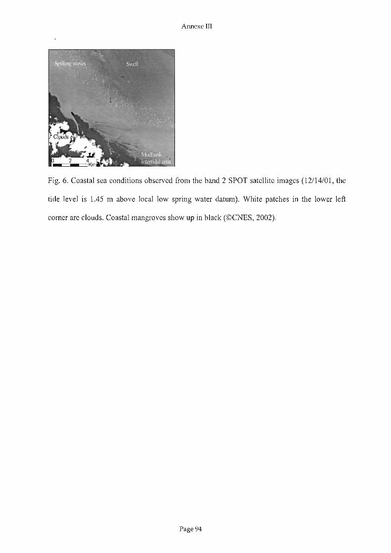
Annexe III
Fig. 6. Coastal sea conditions observed from the band 2 SPOT satellite images (12/14/01, the
tide level is 1.45 m above local low spring water datum). White patches in the lower left
corner are cIouds. Coastal mangroves show up in black (©CNES, 2002).
Page 94

Annexe III
~'E-0.2 r-;:::====='===:---.....,....-~~~-----:-/\~Iî-0.1 .j-= ~~~~ank ~ .
.=l EROSION \. 1~ 0.0 . \ " .Ql COLONISATION J 1~ 0.1 -\- .
~ a.III -0 .2 L.....-..-__............ ............__............ ---'-.........--J
E 1960 1970 1980 1990 2000
1965 1990 1995 2000 2005
- GardelGrallotln prou.Froiderond et al. 1988
L-= Aerial photo ra hy
b.
.$l'È~6.0 . ... .co~ 4.0 ' 1- _ -_1E"'"Iii 2.0 ',:...:... ..,....:.... .~ _.D -- --"D:::sEO
1960 1965 1970 1975 1960
c.
A x5 local retch (100 km)
>: --e- s no licreICh(1.5~Okm~ 0.6 '
~06 ~ .
. - - . - . - . -6- - . .
s c. t:> {:,.~.c..
....'111
MS 0.4 ...
~O- 0.2
200019901980years
1970
oL.....-..-_ _ ~ ~_ _ ~ ~_....J
1960
Fig . 7. Long-tenn geomorphic trends of part of the French Guiana shoreline; (a) cross-shore
evolution of the mangrove shoreline from 1990 to 2002 (from Gardel and Gratiot in press
b); (b) alongshore mud bank migration from 1960 to 2002 along the Cayenne-Kourou
shoreline; (c) Evolution of local and synoptic wave forcing parameters since 1964.
Page 95