dynamics of saltwater intrusion processes in saturated
TRANSCRIPT

Dynamics of Saltwater Intrusion Processes in Saturated Porous Media Systems
by
Sun Woo Chang
A dissertation submitted to the Graduate Faculty of Auburn University
in partial fulfillment of the requirements for the Degree of
Doctor of Philosophy
Auburn, Alabama December 8, 2012
Keywords: saltwater intrusion, density-dependent flow, climate change
Copyright 2012 by Sun Woo Chang
Approved by
T. Prabhakar Clement, Committee Chair, Arthur H. Feagin Professor of Civil Engineering Ming-Kuo Lee, Committee member, Professor of Geology
Xing Fang, Committee member, Associate Professor of Civil Engineering Jose G. Vasconcelos, Committee member, Assistant Professor of Civil Engineering

ii
Abstract
The overarching goal of this dissertation is to contribute towards a better understanding
of the dynamics of saltwater intrusion and the associated transport processes in coastal
groundwater systems. As a part of this effort, we have also investigated the impacts of various
climate-change impacted variables such as average sea level and regional recharge fluxes on
saltwater intrusion processes. Climate change effects are expected to substantially raise the
average sea level. It is widely assumed that sea-level rise would severely impact saltwater
intrusion processes in coastal aquifers. In the first phase of this study we hypothesize that a
natural mechanism, identified here as the ‘‘lifting process,’’ has the potential to mitigate, or in
some cases completely reverse, the adverse intrusion effects induced by sea-level rise. A
detailed numerical study using the MODFLOW-family computer code SEAWAT was completed
to test the validity of this hypothesis in both confined and unconfined systems. Our conceptual
simulation results show that if the ambient recharge remains constant, the sea-level rise will have
no long-term impact (i.e., it will not affect the steady-state salt wedge) on confined aquifers. Our
transient confined-flow simulations show that a self-reversal mechanism, which is driven by the
lifting of the regional water table, would naturally drive the intruded saltwater wedge back to the
original position. In unconfined systems, the lifting process would have a lesser influence due to
changes in the value of effective transmissivity. A detailed sensitivity analysis was also
completed to understand the sensitivity of this self-reversal effect to various aquifer parameters.

iii
The outcomes of the first phase of this research indicated that the changes in groundwater
fluxes due variations in rainfall patterns is one of the major climate-change-induced hydrological
variable that can impact saltwater intrusion in coastal aquifers. In the second phase of this study,
we use a combination of laboratory experiments and numerical simulations to study the impacts
of changes in various types of groundwater fluxes on saltwater intrusion dynamics. We have
completed experiments in a laboratory-scale sand tank model to study the changes in two types
of groundwater fluxes— areal-recharge flux and regional flux. The experimental results were
modeled using the numerical code SEAWAT. The transient datasets collected in this
experimental study are found to be useful benchmark data for testing numerical models that
employ flux-type boundary conditions. Also, based on the experimental observations we
hypothesized that when the fluxes are perturbed it would require relatively less time for a salt
wedge to recede from an aquifer when compared to the time required for the wedge to advance
into the aquifer. This rather counter-intuitive hypothesis implies that saltwater intrusion and
receding processes are asymmetric and the time scales associated with these processes will be
different. We use a combination of laboratory and numerical experiments to test this hypothesis
and use the resulting dataset to explain the reason for the difference in salt wedge intrusion and
recession time scales.
In coastal aquifers, presence of a salt wedge divides the groundwater flow system into
two distinct regions which includes a freshwater region above the wedge and saltwater region
below the wedge. Typically, the freshwater transport processes occurring above a wedge are
much faster than the saltwater transport processes occurring beneath the wedge. Recently, many
modeling and laboratory studies have investigated the movement of salt wedges and the
associated transport processes. Most of these transport studies, however, have focused on

iv
understanding the groundwater plume transport above a wedge. As per our knowledge, so far no
one has completed controlled laboratory experiments to study the transport processes occurring
beneath a saltwater wedge. In this study, we have completed contaminant transport experiments
to map the dynamics of saltwater flow patterns beneath a wedge and relate it to the freshwater
flow patterns present above the wedge. We used a novel experimental approach that employed
variety dyed neutral density tracers to map the mixing and transport processes occurring above
and below a salt wedge. The experimental datasets were simulated using the SEAWAT code.
The model was then used to investigate contaminant transport scenarios occurring beneath a
saltwater wedge in larger field-scale problems.

v
Acknowledgments
I would like to acknowledge my advisor, Dr. T. Prabhakar. Clement for his support and
mentorship. My achievements are evidence of his mentorship and only a small portion of why
he is a named outstanding mentor. I would like to thank to my committee members, Dr. Ming-
Kuo Lee, Dr. Xing Fang, Dr. Jose. G. Vasconcelos and also thank to Dr. Joel G. Melville. I
would like to thank to Dr. Mark Dougherty for giving useful suggestions and for careful edit of
my dissertation. I also thank to Dr. Kang-Kun Lee, Dr. Matthew Simpson, Dr. Rohit Goswami,
and the reviewers of Water Resources Research and Advances in Water Resources. This work
was, in part, supported by the Samuel Ginn College of Engineering Dean Fellowship and by the
Civil Engineering Teaching Assistantship. Finally, I would like to dedicate this work to my
family.

vi
Table of Contents
Abstract ...................................................................................................................................................... ii
Acknowledgments .................................................................................................................................... v
List of Tables ................................................................................................................................ x
List of Illustrations ....................................................................................................................... xi
Chapter 1
INTRODUCTION .................................................................................................................................... 1
1.1 Fundamentals of Saltwater Intrusion ........................................................................ 1
1.2 Impacts of Climate Change on Saltwater Intrusion Processes.................................... 4
1.3 Objectives ................................................................................................................... 5
Chapter 2
INVESTIGATION OF THE IMPACT OF SEA-LEVEL RISE ON SALTWATER INTRUSION PROCESSES - A CONCEPTUAL MODELING STUDY ................................................... 8
2.1 Introduction ............................................................................................................... 8
2.2 Problem Formulation and Conceptual Modeling ..................................................... 11
2.3 Details of Numerical Experiment ............................................................................ 14
2.4 Results ...................................................................................................................... 17
2.4.1 Impacts of Sea-level Rise on Confined Flow Conditions ......................... 17
2.4.2 Sensitivity Analysis of the Self-reversal Process in Confined Systems .... 23
2.4.3 Impacts of Sea-level Rise on Unconfined Aquifers ................................... 29

vii
2.5 Conclusions .............................................................................................................. 35
Chapter 3
INVESTIGATION OF SALTWATER INTRUSION PROCESSES USING LABORATORY EXPERIMENTS INVOLVING FLUX-TYPE BOUNDARY CONDITIONS .............. 37
3.1 Introduction ............................................................................................................. 37
3.2 Method .................................................................................................................... 40
3.2.1 Experimental Approach ............................................................................ 40
3.2.2 Numerical Modeling Approach ................................................................ 43
3.3 Results ...................................................................................................................... 45
3.3.1 Regional Flux Experiment ........................................................................ 45
3.3.2 Areal-recharge Flux Experiment ............................................................... 50
3.3.3 Analysis of Time Scales Associated with Intruding and Receding Salt Wedge Transport Processes ............................................................................... 54
3.4 Conclusions ............................................................................................................... 64
Chapter 4
LABORATORY AND NUMERICAL INVESTIGATION OF TRANSPORT PROCESSES OCCURING BENEATH A SALTWATER WEDGE. .................................................. 66
4.1 Introduction ............................................................................................................. 66
4.2 Methods .................................................................................................................... 72
4.2.1 Experimental Method................................................................................. 72
4.2.2 Details of Tracer Transport Experiments ................................................... 73
4.2.2 Numerical Modeling Method ..................................................................... 74
4.3 Results .................................................................................................................................78
4.3.1 Transport of Tracer Slugs Injected above the Wedge ................................ 78
4.3.2 Characterizing Tracer Transport Patterns beneath a Saltwater .................. 81

viii
4.3.3 Sensitivity of Recirculating Saltwater Flux to Dispersion and the Type of Boundary Condition ................................................................................... 86
4.4 Conclusions ............................................................................................................. 91
Chapter 5
CONCLUSIONS AND RECOMMENDATIONS ..................................................................... 93
6.1 Summary and Conclusions ....................................................................................... 93
6.2 Recommendation for Future Work ........................................................................... 95
Appendix 1 Transient Variations in the Toe Position (XT) for 10%, 50% and 90% Isochlor of Saltwater Wedge ............................................................................................................. 97
Appendix 2 Comparison of Salt-wedge between Central-difference and Upstream-weighting for density-weighting scheme ............................................................................................... 98
Appendix 3 Comparison of Salt-wedge between FDM and TVD scheme ................................ 99
Appendix 4 Analytical Comparison of Salt-wedge Toe Position in Unconfined and Confined Aquifers......................................................................................................................... 100
Appendix 5 Derivation of Dimensionless of Henry problem Parameters and Application to Modified Henry Problem with Areal-recharge flux ...................................................... 102
Appendix 6 Development of Two-dimensional Numerical Code for Simulating Saltwater Transport in Groundwater Systems .............................................................................. 106
Appendix 7 Code Formulation based on TVD scheme for Advection Package ...................... 128
References ................................................................................................................................ 133

ix
List of Tables
Table 2.1 Aquifer properties and hydrological properties used for the base-case problem ....... 16
Table 3.1 Summary of numerical model parameters .................................................................. 44
Table 3.2 Summary measured and modeled flows ..................................................................... 44
Table 4.1 Model parameters used for simulating the lab problem ............................................. 75
Table 4.2 Model parameters used for simulating the field problem (modified from Chang et al.
2011) ............................................................................................................................... 76

x
List of Illustrations
Figure 1.1. Groundwater flow patterns near a pumping well in a coastal aquifer (USGS, 2000) 3
Figure 2.1. Comparison of conceptual models used for visualizing the impacts of sea-level rise
on a saltwater wedge: (a) salt wedge profile after sea-level rise based on a traditional
conceptual model that ignores the lifting effect and (b) a new conceptual model that
includes the lifting effect. ......................................................................................... 13
Figure 2.2. Comparison of steady-state salt wedges predicted before and after the sea-level rise in
the confined system................................................................................................... 20
Figure 2.3. Transient salt wedge profiles for the confined system ............................................. 21
Figure 2.4. Transient variations in the toe position (XT) and freshwater head (hf) at the inland
boundary. .................................................................................................................. 22
Figure 2.5. Sensitivity of the toe position (XT) to (a) specific storage, (b) the magnitude of sea-
level rise, (c) the rate of sea-level rise velocity and (d) the dispersivity coefficients ..
................................................................................................................................... 26
Figure 2.6. Sensitivity of the toe position (XT) to: (a) hydraulic conductivity and (b) freshwater
flux. ........................................................................................................................... 28
Figure 2.7. Comparison of steady-state salt wedges predicted before the sea-level rise (sea level
at 30m) in the unconfined- and confined-flow systems ............................................ 32
Figure 2.8. Comparison of steady-state salt wedges predicted before the sea-level rise in the
unconfined system, after the sea-level rise in the unconfined system, and in an
equivalent 34-m thick confined-flow system ............................................................ 33

xi
Figure 2.9. Comparison of transient variations in toe positions (XT) predicted for the confined
and unconfined flow systems.. .................................................................................. 34
Figure 3.1. Schematic diagram of the (a) regional-flux and (b) areal-recharge flux experiments
and (c) photograph of laboratory setup. .................................................................... 42
Figure 3.2. Transient variations in the salt-wedge patterns due to changes in the regional flux at
the right boundary. The top figure shows intruding transport conditions when the flux
was reduced from 0.833 cm3/s to 0.467 cm3/s, and the bottom figure shows receding
transport conditions when the flux was increased from 0.467 cm3/s to 0.833 cm3/s .
................................................................................................................................... 47
Figure 3.3. Comparison of experimental data model predictions of transient salt wedges for the
regional-flux system: a) advancing-wedge experiment, and b) receding-wedge
experiment................................................................................................................. 48
Figure 3.4. Comparison of experimental and model-simulated toe positions estimated at 0.75 cm
above tank bottom in the regional-flux experiment. ................................................. 49
Figure 3.5. Transient variations in the salt-wedge patterns due to changes in the areal flux values.
The top figure shows intruding transport conditions when the flux was reduced from
1.133 cm3/s to 0.733 cm3/s, and the bottom figure shows receding transport
conditions when the flux is increased from 0.733 cm3/s to 1.133cm3/s ................... 51
Figure 3.6. Comparison of experimental data model predictions of transient salt wedges for the
areal-flux system: a) advancing-wedge experiment, and b) receding-wedge
experiment................................................................................................................. 52
Figure 3.7. Comparison of experimental and model-simulated toe positions estimated at 0.75 cm
above tank bottom in the areal-flux experiment ....................................................... 53
Figure 3.8. Comparison of toe migration rates for intruding and receding wedges for laboratory-
scale problem of (a) regional flux experimental problem and (b) field scale problem
(reported in Chang et al. 2011) ................................................................................. 57

xii
Figure 3.9. Comparison of toe migration rates for intruding and receding wedges for laboratory-
scale problem of areal-recharge flux experimental problem .................................... 58
Figure 3.10. Simulated steady-state velocity fields for the regional flux experiment (a) SS1 and
(b) SS2 ...................................................................................................................... 61
Figure 3.11. Simulated transient velocity fields for the regional flux experiment (a) 2 minutes
after SS1 and (b) 2 minutes after SS2 ....................................................................... 62
Figure 3.12. Visualization of the velocity fields near the salt wedge plotted in log scale at (a) SS1,
(b) 2 minutes after SS1, (c) SS2, and (d) 2 minutes after SS2 .................................. 63
Figure 4.1. Conceptual model illustrating various types of contaminant transport processes
occurring in a coastal groundwater system ............................................................. 67
Figure 4.2. Schematic diagram of the physical model used in this study ................................. 77
Figure 4.3. Comparison of observed data with numerical predictions for the neutral plume
transport experiment (Top figure: lab data; Bottom figure: SEAWAT predictions
with color filled contour -- red > 20 %; yellow 20-14 %; green 14-8 %; and turquoise
8-1 %; also, white line is the 50% saltwater contour of the wedge ......................... 80
Figure 4.4. Comparison of observed data with numerical predictions for the dense plume
transport experiment (Top figure: lab data; Bottom figure: SEAWAT predictions
with color filled contour -- red > 20 %; yellow 20-14 %; green 14-8 %; and turquoise
8-1 %; also, white line is the 50% saltwater contour of the wedge ......................... 80
Figure 4.5. Comparison of observed data with numerical predictions for the transport experiment
completed beneath the wedge (Top figure: lab data; Bottom figure: SEAWAT
predictions with color filled contour -- red > 20 %; yellow 20-14 %; green 14-8 %;
and turquoise 8-1 %; also, white line is the 50% saltwater contour of the wedge ... 84
Figure 4.6. Model simulated results illustrating the transport processes occurring above and
below the saltwater wedge for the field-scale test problem: (a) simulations for low

xiii
regional flow of 0.105 m3/day and (b) simulations for high regional flow of 0.210
m3/day. Initial contaminant concentration at the sources was 100 kg/m3 ................ 85
Figure 4.7. Relationship between freshwater flow and recirculate-saltwater flow for regional and
areal recharge problems with different dispersivity values ...................................... 89
Figure 4.8. Non-dimensional analysis of the relationship between freshwater and saltwater fluxes
[The symbols indicate the following literature data points: + from Chang et al. (2011)
study, � regional flux experimental data from Chang and Clement (2012), � areal
flux experiment data from Chang and Clement (2012), � Cyprus case study from
Destouni and Prieto (2003), � Israel case study from Destouni and Prieto (2003)]
................................................................................................................................... 90

1
Chapter 1
INTRODUCTION
1.1 Fundamentals of Saltwater Intrusion
Groundwater is an important freshwater resource used extensively for water supply.
Groundwater also supports industrial activities in many areas that have limited number of surface
water resources. Unlike a surface water reservoir, which is a concentrated source that can serve
only a narrow region, groundwater is a distributed source which can serve populations
distributed over a larger region. If the areas where groundwater is present coincided with areas
of demand, groundwater can be made available to the local public without any major investment
in water transmission infrastructure. Groundwater is also a relatively stable source since climate
fluctuations induce relatively small variations in groundwater levels in most cases; large volumes
of water stored in groundwater aquifers may serve as a buffer to supply water during lengthy
drought periods [Bear and Cheng, 2010] .
Currently, within the US, it has been estimated that groundwater aquifers located along
the Atlantic Coast supply drinking water to over 30 million residents living in coastal towns from
Maine to Florida [USGS, 2000]. These precious coastal aquifers are constantly being
contaminated by saline water through a natural process known as saltwater intrusion. Figure 1.1
illustrates the dynamics of groundwater flow and mixing of freshwater and saltwater in a coastal
aquifer. As shown in the figure, the fresh groundwater region is in direct contact with the saline
seawater region in coastal aquifers. Under natural conditions, a dynamic equilibrium exists
between these two regions. There are numerous human and environmental factors that can
adversely impact this equilibrium and that lead to severe saltwater contamination of the

2
freshwater region. Once contaminated, it is difficult and expensive to clean up saltwater
contaminated aquifers. In some cases the contamination could even be irreversible [Bear and
Cheng, 2006].
Saltwater intrusion into freshwater aquifers primarily occurs due to the difference in the
density of seawater (which has a density value of 1.025 g/cm3) and fresh groundwater (which has
a density value of 1.000 g/cm3). This small density difference can play a significant role in
controlling two types of saltwater intrusion processes: lateral intrusion of seawater beneath the
regional aquifer and up-coning of seawater near pumping wells. The up-coning of seawater
normally occurs near a pumping well when a large amount of groundwater is withdrawn from
the aquifer. Anthropogenic pumping activities induce a cone of depression around the well,
which can lead to upward migration of seawater directly into pumping wells. Lateral intrusion of
seawater, on the other hand, would occur naturally when denser saltwater seeps inland at the
bottom of the freshwater aquifer (see Figure 1.1). Lateral intrusion of seawater would result in a
distinct curved interface that separate the freshwater and saltwater regions; this interface is
known as the regional “saltwater wedge.” The shape and extent of the interface is determined by
various factors such as the geology of the aquifer, climate patterns, variations in natural
groundwater flow and the sea level, etc.

3
Figure 1.1. Groundwater flow patterns near a pumping well in a coastal aquifer (USGS, 2000)

4
1.2. Impacts of Climate Change on Saltwater Intrusion Processes
In recent years, population growth and land use changes in coastal areas have increased
the demand for freshwater; in addition, it is believed that climate change effects have further
reduced the water availability in coastal areas [Ranjan et al., 2006]. Climate change could lead
to rise in sea levels, and climate change could also alter groundwater recharge fluxes due to
changes in rainfall patterns. Droughts induced by climate change would result in reduction of
regional freshwater recharge and this would enhance saltwater intrusion. In the published
literature, climate change models have forecasted significant sea-level rise ranging from 0.18 to
0.51 m by the end of this century [IPCC, 2007]. According to Titus et al. (2009), during the
twentieth century the majority of Atlantic Coast and Gulf of Mexico Coast regions experienced
rates of sea-level rise ranging from 2 to 10 mm/year. These estimates are considerably higher
than the current global average of 1.7 mm/year, and have led to the concern that rising oceans
levels would impact the quality of both surface and ground water supplies and reduce the world’s
existing fresh water reserves. Impact of climate change on saltwater intrusion in coastal
groundwater systems is a serious environmental concern since eighty percent of the world
population resides along the coastal regions and depends on coastal aquifers for their water
supply. Most of these regions have water-scarce coastal towns that have limited freshwater
supply, and are also undergoing rapid population growth. Saltwater intrusion is an important
concern for these towns.
Researchers have used modeling studies to understand the coupling of climate change
effects with groundwater problems. Dausman and Langevin (2005) evaluated the relative
importance of drought, well-field pumping, sea-level rise, and canal management on saltwater
intrusion for the Biscayne aquifer in Southern Florida. The simulation results for a coastal

5
aquifer in Broward County, Florida, demonstrated that if the sea-level rise becomes greater than
48 cm over the next 100 years local well fields would be vulnerable to chloride contamination.
Aquifers in small barrier islands are particularly more vulnerable to climate change effects than
other aquifers because extreme events such as hurricanes can deposit abnormal amount of salt by
directly inundating these islands. Gillett et al. [2000] reported that the occasional hurricanes that
strike the Gulf Coast can cause tidal surges up to 5 to 25 feet above the normal level. These
storm surges could dump large amount of saltwater over sandy soil and contaminate the shallow
groundwater. In addition to storm surges, catastrophic events such as tsunamis can also dump
large volume of saltwater above freshwater coastal aquifers. Ilangasekare et al. (2006) discuss a
detailed field survey completed in Sri Lanka that documented saltwater intrusion caused by the
tsunami wave generated by the 2004 Indian Ocean earthquake on Sunday, 26 December 2004,
with an epicenter off the west coast of Sumatra, Indonesia. The tsunami surge not only caused
the salt wedge to temporarily move inward, but it also dumped a dense seawater directly over
sandy unconfined aquifer along the entire Sri Lankan coast. Ilangasekare et al. (2006) used a
combination laboratory analysis together with simple analytical calculations to estimate the time
taken to naturally restore these aquifers. These field studies have demonstrated the importance
of understanding impacts of climate change and other extreme hydrological events on saltwater
intrusion processes.
1.3 Objectives
The overall goal of this research is to develop a better understanding of the dynamics of
saltwater intrusion processes in coastal groundwater aquifers. This study has four research
objectives, and this dissertation has four distinct chapters that document the results of

6
investigations related to each of these objectives. Each of the four chapters is organized in a
journal format and has an introduction section and also reviews all relevant literature.
The first objective of this study is to investigate the transient impacts of the sea-level
rise on saltwater intrusion processes in confined and unconfined coastal aquifers that are
driven by natural recharge fluxes. The results of this numerical study are used to develop an
intuitive understanding for saltwater intrusion dynamics, which can help better manage the
potential long term impacts of sea-level rise on coastal aquifers.
The result of the first phase of this study demonstrated the importance of flux-type
boundary conditions. Our review indicated that past experimental efforts related to saltwater
intrusion processes have primarily focused on conducting experiments involving constant head
boundary conditions. Therefore, the second objective of this work is to conduct
experimental studies to investigate the dynamics of saltwater intrusion processes in an
unconfined aquifer using different types of flux boundary conditions. We investigated the
influence of variations in recharge patterns (resulting from changes in rainfall conditions) on a
transient movement salt wedge using a laboratory-scale aquifer model and modeled the data
using a numerical code. Both the laboratory data and the numerical simulations were used to
develop a better understanding of the dynamics of salt wedges under transient flow conditions.
Many of the shallow unconfined aquifers in coastal areas are contaminated by various
type of contaminants released from a variety of anthropogenic sources [Westbrook et al., 2005].
Furthermore, regional groundwater flow can also transport large amount of nutrients, which then
could be exchanged across the salt wedge. Therefore, the third objective of this work is to
conduct laboratory experimental studies to investigate the contaminant transport processes
near a salt wedge. We completed laboratory experiments to study tracer transport in both

7
freshwater and salt water flow zones in the vicinity of the salt wedge. The results were used to
analyze contaminant transport scenarios above and below a saltwater wedge.
This dissertation has five chapters. The first chapter (the current chapter) provides a
basic introduction to this research, lists the objectives, and provides a brief summary of each
chapter. The second chapter focuses on the first objective, with the outcome of this effort
already published in Advances in Water Resources [Chang et al., 2011]. The third chapter
focuses on the second objective and the outcome of this effort has been accepted in Water
Resources Research [Chang and Clement, 2012b]. The fourth chapter focuses on the third
objective and the outcome of this effort has been communicated to Journal of Contaminant
Hydrology [Chang and Clement, 2012a] The fifth chapter provides a brief summary of the key
outcomes of this research and offers recommendations for future work.

8
Chapter 2
INVESTIGATION OF THE IMPACT OF SEA-LEVEL RISE ON SALTWATER INTRUSION
PROCESSES - A CONCEPTUAL MODELING STUDY
2.1 Introduction
Saltwater intrusion is a serious environmental issue since eighty percent of the world’s
population live along the coast and utilizes local aquifers for their water supply. In the US alone,
it is estimated that freshwater aquifers along the Atlantic coast supply drinking water to 30
million residents living in coastal towns located from Maine to Florida [USGS, 2000]. Under
natural conditions, these coastal aquifers are recharged by rainfall events, and the recharged
water flowing towards the ocean would prevent saltwater from encroaching into the freshwater
region. However, over exploitation of coastal aquifers has resulted in reducing groundwater
levels (hence reduced natural flow) and this has led to severe saltwater intrusion. Cases of
saltwater intrusion, with varying degrees of severity and complexity, have been documented
throughout the Atlantic coastal zone. For example, in May County, New Jersey, more than 120
water supply wells have been abandoned because of saltwater contamination [Lacombe and
Carleton, 1992]. A recent USGS [2000] study provides a summary of saltwater intrusion
problems and various mitigation techniques. International organizations have identified
saltwater intrusion as one of the major environmental issues faced by several coastal cities in
India, China, and Mexico [WWD, 1998]. Researchers have also reported that variations in the
sea level and the associated wedge movement can influence the near-shore and/or large-scale
submarine discharge patterns and impact nutrient loading levels across the aquifer-ocean

9
interface [Li and Jiao, 2003b; Li et al., 2008; Li et al., 1999; Michael et al., 2005; Robinson et al.,
2007]. Therefore, understanding the dynamics of saltwater intrusion in coastal aquifers and its
interconnection to anthropogenic activities is an important environmental challenge.
While anthropogenic activities such as over pumping and excess paving in urbanized
areas are the major causes of saltwater intrusion, it is anticipated that increases in sea level due to
climate change would aggravate the problem. Nevertheless, only a few studies have focused on
understanding the combined effects of climate change and anthropogenic impacts [Li and Jiao,
2003a; b]. Feseker [2007] completed a numerical modeling study to assess the impacts of
climate change and changes in land use patterns on the salt distribution in a coastal aquifer. The
model used parameters to reflect the conditions similar to those observed at the CAT-field site
located in the northern coast of Germany. The study concluded that rising sea level could induce
rapid progression of saltwater intrusion. Furthermore, the time scale of changes resulting from
the altered boundary conditions could take decades or even centuries to impact groundwater
flows and hence the present day salt distribution might not reflect the long term equilibrium
conditions. Leatherman [1984] investigated the effects of rising sea-level on salinization in an
aquifer in Texas. Meisler et al.[1985] used a finite-difference computer model to analyze the
effect of sea-level changes on the development of the transition zone between fresh groundwater
and saltwater in the northern Atlantic Coastal Plain (from New Jersey to North Carolina). Navoy
[1991] studied aquifer-estuary interactions to assess the vulnerability of groundwater supplies to
sea level rise-driven saltwater intrusion in a coastal aquifer in New Jersey. Oude Essink [2001]
used a three-dimensional transient density-driven groundwater flow model to simulate saltwater
intrusion in a coastal aquifer in the Netherlands for three types of sea-level rise scenarios: no
rise, a sea-level rise of 0.5 m per century, and a sea-level fall of 0.5 m per century. They

10
concluded that sea-level rise of 0.5 m per century would increase the salinity in all low-lying
regions closer to the sea. Dausman and Langevin [2005] completed SEAWAT simulations for a
coastal aquifer in Broward County, Florida, and demonstrated that if the sea-level rise becomes
greater than 48 cm over the next 100 years then several local well fields would be vulnerable to
chloride contamination. Melloul and Collin [2006] evaluated the potential of sea-level rise to
cause permanent freshwater reserve losses in a coastal aquifer in Israel. They quantified the
saltwater intrusion effect due the lateral movement of seawater and due changes in the
groundwater head. For the assumed sea-level rise of 0.5 m, about 77% of the loss was due to the
lateral movement and about 23% was due to the head change. Ranjan et al. [2006] used the
sharp interface assumption to analyze the effects of climate change and land use on coastal
groundwater resources in Sri Lanka. Giambastiani et al. [2007] conducted a numerical study to
investigate saltwater intrusion in an unconfined coastal aquifer of Ravenna, Italy. Their result
showed that the mixing zone between fresh and saline groundwater will be shifted by about 800
m farther inland for a 0.475 m per century of sea-level rise. Loaiciga et al. [2011] employed
hydrogeological data and the finite-element numerical model FEFLOW to assess the likely
impacts of sea-level rise and groundwater extraction on seawater intrusion in the Seaside Area
aquifer of Monterrey County, California, USA. Sea-level rise scenarios were consistent with
current estimates made for the California coast, and varied between 0.5 and 1.0 m over the 21st
century. These authors concluded that sea-level rise would have a minor contribution to seawater
intrusion in the study area compared to the contribution expected from groundwater extraction.
The primary focus of most of the field-scale modeling studies discussed above was to
understand saltwater intrusion problems related to a specific field site. More recently, Werner
and Simmons [2009] completed a conceptual modeling study using a steady-state, sharp-

11
interface analytical model focused on developing a general understanding of the impacts of sea-
level rise on groundwater aquifers that might have different types of boundary conditions. They
used a relatively simple analytical model to provide a first-order assessment of the impacts of sea
level changes on saltwater intrusion on aquifer systems with two types of boundary conditions.
Their results showed that the level of intrusion would depend on the type of inland boundary
condition assumed in the model. The steady-state, sharp-interface, analytical expression used in
the study did not consider saltwater mixing effects and transient effects. The transient effects in
unconfined aquifers were later investigated by Webb and Howard [2010], using a numerical
model that employed constant head boundary conditions to study the changes in the rates of
intrusion for a range of hydro-geological parameters.
The objective of this study is to complete a comprehensive investigation of the transient
impacts of sea-level rise on saltwater intrusion processes in both confined and unconfined coastal
aquifer systems that are driven by natural recharge fluxes. The results are then used to develop
an intuitive understanding of saltwater intrusion dynamics, which can help better assesses and
manage the potential long term impacts of sea-level rise on coastal aquifers.
2.2 Problem Formulation and Conceptual Modeling
Under natural flow conditions, dense sea water would have the tendency to intrude
beneath fresh groundwater. The spatial extent of the intruded saltwater wedge (designated as the
“toe position XT”) would depend on several aquifer parameters including recharge rate, regional
aquifer discharge rate, hydraulic properties, and sea level. Recent climate change studies have
shown that the global sea-level, on average, is expected to rise between 18 and 59 cm this
century [IPCC, 2007]. Worst-case projections show it could be as high as 180 cm [Vermeer and

12
Rahmstorf, 2009]. Therefore, environmental planners worldwide are concerned about the
impacts of sea-level rise on saltwater intrusion processes, especially in over-utilized, urbanized
coastal aquifers that already have low groundwater levels. Currently, it is expected that the
rising sea level will enhance saltwater intrusion and potentially contaminate many freshwater
reserves. Figure 2.1a depicts a commonly assumed conceptual model [Cheng et al., 2000;
Custodio and Bruggeman, 1987; Fetter, 2001; Mantoglou, 2003; Strack, 1976; Werner and
Simmons, 2009] that illustrates how the rising sea level would impact the groundwater quality by
forcing the wedge to migrate inland. This conceptual model, however, ignores the fact that when
the seawater rises at the sea-side boundary the system would pressurize and the water-table level
might be “lifted” throughout the aquifer. Figure 2.1b illustrates a revised conceptual model.
This revised model accounts for the lift in the groundwater level over the entire system due to the
changes in the sea-side boundary condition. It is expected that after a long period (i.e., at or near
steady state) this lifting effect would approximately raise the entire fresh water body (measured
from the bottom of the aquifer) by an extent similar to the sea-level rise (i.e., a similar order of
magnitude). One could intuitively expect this lifting mechanism to counteract and reduce the
impacts due to the sea-level rise. However, it is unclear to what extent this lifting process could
reduce the overall impacts due to sea-level rise. In this study, we employ this revised conceptual
model to hypothesize that changes in the sea-level might have little or no impact on saltwater
intrusion when the net flux through the system is unchanged. The overall goal of this conceptual
study is to test the validity of this hypothesis, and understand its ramifications under transient
conditions in idealistic confined and unconfined systems.

13
Figure 2.1. Comparison of conceptual models used for visualizing the impacts of sea-level rise
on a saltwater wedge: (a) salt wedge profile after sea-level rise based on a traditional conceptual
model that ignores the lifting effect, and (b) a new conceptual model that includes the lifting
effect.
Regional flow, Q
Expected intrusion level
Recharge, W
( a )
New Sea Level
Old Sea Level
Wedgebefore rise
Wedge after rise
Regional flow, Q
New Groundwater LevelOld Groundwater LevelNew Sea Level
Old Sea Level
Expected intrusion levelafter accounting for groundwater table rise
Wedgebefore rise
( b )
Recharge, W
Wedge after rise

14
2.3 Details of Numerical Experiment
The base-case problem considered in this study was adapted from Werner and Simmons’
conceptual model [Werner and Simmons, 2009] of a seawater intrusion field study completed in
Pioneer Valley, Australia. The original problem only considered unconfined flow conditions; in
this work, the problem was modified to investigate both confined and unconfined conditions.
Our numerical study considered a two-dimensional aquifer system which is 1000 m long and 30
m thick. A rectangular numerical grid, with ∆x = 4 m, ∆y = 1 m and ∆z = 0.4 m, was used. The
initial sea level (prior to the rise) was assumed to be at 30 m and the sea level was then allowed
to rise instantaneously to 34 m. The net sea-level rise assumed was 4 m, a theoretical worst-case
scenario which is approximately double the extreme value predicted by Vermeer and Rahmstorf
[2009]. The assumed sea-level rise was chosen to approximately mimic the last interglacial
period’s rapid sea-level rise that reached up to 4 to 6 m due to rapid loss of ice-sheet [Blanchon
et al., 2009]. It is important to note that this is not a “true” scenario simulation exercise; our
objective is not to forecast the future location of saltwater wedge for a specific system, rather it is
to develop a generic conceptual understanding to assess the potential impacts of sea-level rise on
saltwater intrusion processes. Therefore, some extreme sea-level rise scenarios were initially
simulated (as the base-case) to better illustrate certain subtle transport mechanisms. Later, as a
part of the sensitivity analysis, we explore some realistic sea-level rise scenarios that range from
0.2 m (minimum rise predicted by IPCC) to 4 m (double the maximum rise predicted by
Vermeer and Rahmstorf [2009] ). Also, in all base-case simulations we assumed instantaneous
rise (a worst-case scenario) and later in the sensitivity section we have presented the results for
other finite rates of sea-level rise.

15
The seawater density was assumed to be 1,025 kg/m3 with salt concentration of 35 kg/m3.
The regional groundwater flux supplied through the inland boundary using a set of artificial
injection well nodes. The flux (q, flow per unit depth) supplied from the right boundary was
0.005 m2/day (or a total flow rate (Q) of 0.15 m3/day over the 30 m thick aquifer). Recharge (W)
flow was delivered from the top boundary at the rate of 5×10⁻⁵ m/day. These regional and
recharge flows were simply selected to locate the initial location of the saltwater toe in between
300 to 500 m. The hydraulic conductivity was set to 10 m/day, specific storage was set to 0.008
m-1 in each confined layer, and porosity to 0.35. Longitudinal and transversal dispersivity values
were assigned to be 1 m and 0.1 m, respectively. The initial sea level was set at 30 m to simulate
a base-case steady-state wedge. This steady-state wedge was later used as the initial condition in
all subsequent sea-level rise simulations. Impacts of density-weighting schemes (upstream and
central) and various advection schemes (TVD and upstream finite-difference) were investigated
in using tests simulations (results summarized in Appendix 2 and 3). In the final simulations we
used upstream density weighting and the finite difference scheme advection package. Other
model parameters used are summarized in Table 2.1.
The MODFLOW-family variable density flow code SEAWAT [Langevin C et al., 2003]
was used in this study with the central difference weighting option. The modeling approach was
validated by solving Henry’s steady-state solution [Henry, 1964; Simpson and Clement, 2004]
and also laboratory data provided by Goswami and Clement [2007], and Abarca and Clement
[Abarca and Clement, 2009]. Several sets of numerical experiments were completed to explore
various types of flow conditions and parameter values. The first set of experiments only
considered confined-flow conditions and the results were used to explore certain novel salt-

16
wedge reversal mechanisms that have not been reported in the published literature. Later
simulations consider both confined and unconfined flow conditions.
Table 2.1. Aquifer properties and hydrological properties used for the base-case problem.
Property Symbol Value
Horizontal aquifer length L 1000 m
Vertical aquifer thickness B 30 m
Inland groundwater flow rate Q 0.15 m3/day
Uniform recharge rate from top W 5×10⁻⁵ m/day
Hydraulic conductivity K 10 m/day
Specific storage, Ss 0.008 m-1
Longitudinal dispersivity αL 1 m
Transverse dispersivity αT 0.1 m
Saltwater concentration Cs 35 kg/m3
Saltwater density ρs 1,025 kg/m3
Freshwater density ρf 1,000 kg/m3
Porosity n 0.35

17
2.4 Results
2.4.1. Impacts of Sea-level Rise on Confined Flow Conditions
The goal of the first steady-state simulation is to estimate the initial saltwater wedge
profile that would exist in the system prior to sea-level rise. Figure 2.2 (continuous line) shows
the 50% isochlor of the initial steady-state concentration profile for the base-case, confined-flow
system. This 50% concentration profile is defined as the base saltwater wedge. The figure
shows that under the assumed groundwater flow conditions, the toe of the salt wedge advanced
to 382 m into the aquifer before sea-level rise. This steady-state condition was used as the initial
condition in all subsequent simulations.
The second steady-state simulation aimed to predict the long-term salt-wedge profile
after the sea-level rise. The water level at the seaside boundary was abruptly increased from 30
to 34 m to simulate an instantaneous sea-level rise. The system was allowed to evolve for
80,000 days to reach steady-state conditions. The new steady-state solution for the salt wedge
simulated by the model after raising the sea level is also shown in Figure 2.2 (using circle data
points). Interestingly, and rather surprisingly, the model-predicted saltwater profiles for both
conditions (pre and post sea-level rise) were identical, indicating that the sea-level rise will have
no impact on the location of the steady-state wedge when the freshwater flux transmitted through
the system remained constant (i.e., if the rainfall/recharge pattern was not changed). This non-
intuitive result has several important practical implications. The result indicates that the lifting
effect postulated in the conceptual model described in Figure 1c will fully offset the negative
impacts of sea-level rise in constant flux confined flow systems.

18
To further explore this result, we present the transient evolution of the location of the
saltwater wedge in Figure 2.3. These profiles show that when the sea-level was instantaneously
raised, the wedge initially started to move inward; however, after about 8,000 days, the direction
of wedge movement reversed and the wedge started to move backward until it reached the initial
steady-state profile. As far as we are aware, no one has predicted or postulated this self-reversal
mechanism. Understanding this self-reversal process has an enormous implication on how water
resources managers would perceive and manage the impacts of sea-level rise on saltwater
intrusion. 10% isochlor and 90% isochlor shows the same transient movement (See appendix 1)
Figure 2.4 shows the transient variations in the toe position of the saltwater wedge (XT).
The data shows that, under assumed flow conditions, the salt wedge first advanced into the
aquifer for about 8,000 days and reached a maximum distance of 432 m (from the sea boundary)
and then started to recede. The figure also shows the simulated transient freshwater head levels
at the right side boundary. This freshwater head data is an excellent surrogate for quantifying the
progression of the aquifer “lifting” process, postulated in Figure 2.1b. This dataset shows that
the initial head at the right boundary, as predicted by the model prior to the sea-level rise, was 31
m. When the sea-level was raised instantaneously from 30 to 34 m, it took about 2,000 days for
the right boundary to fully respond to this change. After about 2,000 days, the fresh-water level
in the right boundary reached a constant value of about 35 m. The net change in the freshwater
level was about 4 m, almost identical to the sea-level rise forced at the left boundary. This
implies that the raising seaward-boundary head lifted the entire fresh groundwater system by a
similar order of magnitude. This lifting process was able to fully reverse the salt wedge location.
The rate of the reversal process would depend on the rate at which the groundwater system was
lifted (or how quickly the groundwater heads would respond), which would in turn depend on the

19
storage properties of the aquifer and the rate of sea-level rise. In the following section, we
provide a detailed analysis that quantifies the sensitivity of the self-reversal process to the value
of storage coefficient, the rate of sea-level rise and the magnitude of rise. All these simulations
used the base-case steady-state solution as the initial condition.

20
Figure 2.2. Comparison of steady-state salt wedges predicted before and after the sea-level rise in
the confined system.
0
10
20
30
0 200 400 600 800 1000
z (m
)
x (m)
Initial condition
80,000 days, steady state

21
Figure 2.3. Transient salt wedge profiles for the confined system.
0
10
20
30
0 200 400 600 800 1000
z (m
)
x (m)
Initial condition
3,000 days
8,000 days
15,000 days
80,000 days, steady state

22
Figure 2.4 Transient variations in the toe position (XT) and freshwater head (hf) at the inland
boundary.
30
32
34
36
380
400
420
440
460
0 10,000 20,000 30,000 40,000
hf(m
)
XT
(m)
Time (day)
Toe position
Freshwater head

23
2.4.2. Sensitivity Analysis of the Self-reversal Process in Confined Systems
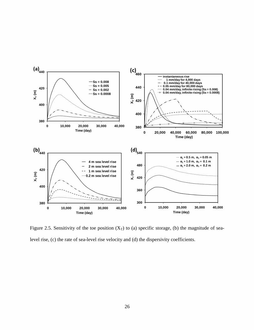
2. 4.2.1. Sensitivity to Specific Storage
We first explored the sensitivity of the intrusion mechanism to various values of specific
storage (Ss). In this analysis, the value of Ss was varied by an order of magnitude with the range
0.0008 to 0.008 m-1. In all sensitivity simulations, the other parameters were fixed at base-case
levels shown in Table 2.1. Figure 2.5a shows the temporal variations in the toe position (XT) for
different values of Ss. The data shows that when Ss was small the system responded rapidly and
the intrusion effect was reversed quickly. Also, the maximum intrusion length was small for
smaller values of Ss. The maximum values of the predicted saltwater toe position (XT) were 432,
412, 394, and 386 m for the Ss values 0.008, 0.005, 0.002 and 0.0008 m-1, respectively. The
figure shows that when Ss is small (at 0.0008 m-1) the change in the salt wedge location was
relatively small even for an extreme sea-level rise of 4 m. The total time required to reach the
maximum intrusion level (defined as the duration of intrusion) was 6,000 to 8,000 days. These
values appear to be relatively insensitive to Ss. Overall, the extent of saltwater intrusion as
indicated by the maximum value of XT was more sensitive to Ss than the duration of intrusion.
2.4.2.2. Sensitivity to the Magnitude of Sea-level Rise
The sensitivity of the intrusion length to the magnitude of the sea-level rise was explored
by varying the sea-level rise within the range of 0.2 to 4 m. Figure 2.5b shows the transient
variations in XT values for various values of sea-level rise. The maximum values of XT were
approximately proportional to the magnitude of sea-level rise. Also, similar to the previous

24
sensitivity experiment, the time taken to reach the maximum values was about 6,000 to 8,000
days, and this time was relatively insensitive to the magnitude of the sea-level rise.
2.4.2.3. Sensitivity to the Rate of Sea-level Rise
Simulations were completed to test the sensitivity of the intrusion process to changes in
the rate of sea-level rise. Literature data indicated that the current rate of sea-level rise observed
worldwide has ranged from 2 to 4 mm/year [McCarthy, 2009]. Climate change model
projections, however, show that the global rate could at least double by the end of this century
[Anderson et al., 2010]. A total rise of 4 m was simulated using six different rate scenarios:
instantaneous, 1 mm/day for 4,000 days, 0.1 mm/day for 40,000 days, 0.05 mm/day for 80,000
days, and infinite rise at a rate of 0.04 mm/day with Ss = 0.008 and Ss = 0.0008. Figure 2.5c
shows the temporal variations in the simulated toe position (XT) for all five scenarios. The data
demonstrates that the rate of the self-reversal process would depend on the sea-level rise rate.
When the rate of rise was low the reversal cycle had a longer duration. The maximum value of
the intrusion length, XT, decreased with decrease in the rate of sea-level intrusion. The time
taken to reach the maximum level of intrusion was 7,500, 10,000, 40,000 and 80,000 days for
instantaneous, 1 mm/day, 0.1 mm/day, 0.05 mm/day sea-level rise rates, respectively. When sea-
level was allowed to rise infinitely at a fixed rate, the results reached an irreversible, quasi
steady-state level. It is important to note this irreversible intrusion level was primarily an artifact
due the relatively large storage value (of 0.008 m-1) assumed as the base-case parameter. When
we reduced the specific storage value by an order of magnitude (to 0.0008 m-1, a more typical
value for confined flow) the head information propagated quickly and the lifting effect became
continuously active. Therefore, the system with a higher Ss value experienced immediate

25
reversal and experienced very little intrusion under the continuous-rise scenario. Overall,
changes in the rate of sea-level rise influenced the maximum level of intrusion as well as the
time required to reach the maximum level. The time required to reach the maximum would, to a
large extent, depended on how long the sea rise occurred.
2.4.2.4. Sensitivity to Dispersivity Values
We explored the sensitivity of the intrusion mechanism to dispersivity coefficients by
varying the value within the range of 0.5 m to 2 m for longitudinal dispersivity, αL, and 0.05 m to
0.2 m for transverse dispersivity, αT. As Abarca et al [2007b] pointed out, changing the values of
dispersivity would impact the value of XT (initial XT decreased when the dispersivity coefficients
were increased). Therefore, we defined a parameter “net change in salt wedge location,” which
was computed as: maximum value of XT - initial position of XT, to quantify the changes. Figure
2.5d shows the temporal variations in the toe position (XT) for different values of dispersivity.
The net change in the salt wedge location was in between 44 and 53 m. The time taken to reach
the maximum intrusion level and the peak of XT values were relatively insensitive to changes in
the value of dispersivity coefficient.
26
Figure 2.5. Sensitivity of the toe position (XT) to (a) specific storage, (b) the magnitude of sea-
level rise, (c) the rate of sea-level rise velocity and (d) the dispersivity coefficients.
380
400
420
440
0 10,000 20,000 30,000 40,000
XT
(m)
Time (day)
Ss = 0.008Ss = 0.005Ss = 0.002Ss = 0.0008
(a)
380
400
420
440
460
0 20,000 40,000 60,000 80,000 100,000X
T(m
)Time (day)
instantaneous rise1 mm/day for 4,000 days
0.1 mm/day for 40,000 days0.05 mm/day for 80,000 days0.04 mm/day, infinite rising (Ss = 0.008)0.04 mm/day, infinite rising (Ss = 0.0008)
(c)
380
400
420
440
0 10,000 20,000 30,000 40,000
XT
(m)
Time (day)
4 m sea level rise2 m sea level rise1 m sea level rise
0.2 m sea level rise
(b)
300
360
420
480
540
0 10,000 20,000 30,000 40,000
XT
(m)
Time (day)
half dispersivityalphaL = 1 malphaL = 2 m
αL = 0.5 m, αT = 0.05 m
αL = 1.0 m, αT = 0.1 m
αL = 2.0 m, αT = 0.2 m
(d)

27
2.4.2.5. Sensitivity to Other Hydrological Parameters
It is important to note that the transient reversal patterns would depend on the values of
hydraulic conductivity, recharge rate and ambient groundwater flow. Sensitivity to variations in
all these model parameters was also explored in this study. Simpler analytical solutions can be
used to intuitively infer the sensitivity to individual variations in K, W and Q values under steady
conditions. Werner and Simmons [Werner and Simmons, 2009] followed this approach and
completed a detailed sensitivity assessment for a steady-state unconfined problem. In this study,
we present the results of a selected number of sensitivity tests completed for a transient confined
aquifer system using SEAWAT. Figure 2.6a shows the transient variations in XT values for
different hydraulic conductivity values; K values used are: 5 m/day, 10 m/day and 15 m/day. It
should be noted that the simulated profiles have different initial XT since individually changing
any one of these parameters (K, W or Q) would alter the steady-state solution of the base
problem. The results show that the peak value of XT (relative to the initial XT value) would
increase, and the responding time would decrease (as expected) when the K value was decreased.
Figure 3.6b shows the transient variations in XT values for various values of Q and W (0.67×base
values: Q = 0.1 m3/day and W = 3.3×10⁻⁵ m/day; base values: Q = 0.15 m3/day and W = 5×10⁻⁵
m/day; doubled the base values: Q = 0.3 m3/day and W = 1×10⁻⁴ m/day). The data show that
when the amount of freshwater flow was increased the peak value of XT increased and system
also had a shorter responding time. It should be noted that if the transport parameters were
scaled consistently (for example, increase K and reduce the Q by a similar factor) then there will
be very little variation in the peak value of XT.

28
Figure 2.6. Sensitivity of the toe position (XT) to: (a) hydraulic conductivity and (b) freshwater
flux.
200
400
600
800
0 10,000 20,000 30,000 40,000
XT
(m)
Time (day)
K = 5 m/day
K = 10 m/day
K = 15 m/day
(a)
200
400
600
800
0 10,000 20,000 30,000 40,000
XT
(m)
Time (day)
base freshwater flux
2 base flux
0.67 base flux
(b)
×
×

29
2.4.3. Impacts of Sea-level Rise on Unconfined Aquifers
To examine the impacts of sea-level rise on unconfined flow conditions, we completed
numerical simulations of an unconfined aquifer with dimensions identical to those used in the
confined simulation, except the top layer was modified to simulate unconfined flow. The length
of the unconfined aquifer was 1,000 m and the total thickness was 35 m. A numerical grid with
∆x = 4 m, ∆y = 1 m and ∆z = 0.4 m (75 confined layers), and a top unconfined layer of ∆z = 5 m
was used. In all unconfined flow simulations, the value of average hydraulic conductivity was set
to 10 m/day, total regional freshwater flow (Q) from the right boundary was set to 0.15 m3/day,
and the areal recharge flux (W) was set to 5×10⁻⁵ m/day. Initially, the regional flow rate was
assigned to 0.0019 m3/day for all confined layers with 0.0048 m3/day for top unconfined layer
(note the top unconfined layer was 1 m as opposed confined nodes which are 0.4 m). After the
sea-level rise, the flow rate was again redistributed over the unconfined zone of 4 m. In order to
redistribute the same flow of 0.15 m3/day over an increased saturated aquifer depth, all the
confined nodes were assigned a flow of 0.0017 m3/day and the top 4-m unconfined layer was
assigned 0.021 m3/day. In order to compare unconfined flow simulation results against confined
flow results, an identical instantaneous sea-level rise (rise from 30 to 34 m) scenario was
assumed. The specific storage, Ss, was set to 0.008 m-1 for all confined layers, and specific yield,
Sy, was set to 0.1 for the top unconfined layer.
We first completed a base-case, steady-state simulation for the unconfined system to generate
the initial conditions that existed prior to the sea-level rise. Figure 2.7 compares the steady-state
salt wedge predicted for the unconfined flow system with the wedge predicted for a similar
confined flow system (data from Figure 2.2). The figure shows the both wedges are almost

30
identical, indicating that both confined and unconfined systems would behave in a similar
manner at steady-state conditions. The similarity between the two steady-state solutions can also
be explained mathematically, as shown in Appendix 5.
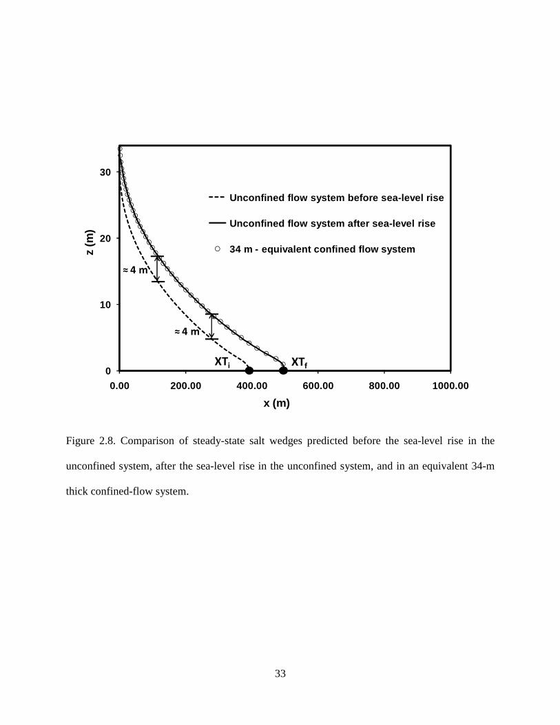
To understand the impacts of sea-level rise on the unconfined aquifer, we instantaneously
raised the sea-level by 4 m and let the system reach steady state. Figure 2.8 compares the initial
and final steady-state saltwater wedge profiles in the unconfined system (dotted and continuous
lines). These profiles show that, unlike the confined system (compare with Figure 3 results), the
saltwater intrusion process is not reversible for the unconfined system. In unconfined aquifers,
the initial location of the toe XTi and the final location of the toe position XTf are distinctly
different. This is because, under unconfined conditions, the sea-level rise increases in the
saturated thickness (or transmissivity) of the aquifer. This increased transmissivity allows the
wedge to penetrate further into the system, resulting in a new steady-state condition. Comparing
the initial and final salt-wedge profiles indicates the initial salt wedge was approximately raised
by 4 m, similar to the level of sea-level rise. The groundwater level also rose over the entire
aquifer by about 4 m (as illustrated in Figure 2.1b), all the way to the inland boundary (the
predicted groundwater raise at the inland boundary was similar to the data shown in Figure 2.4).
These data indicate that the aquifer lifting process is active in the unconfined system. The lifting
process, however, was not able to fully reverse the wedge location since the system evolved from
a steady-state solution for the 30-m thick aquifer (with initial toe, XTi, at about 382 m) to a new
steady-state solution for the 34-m thick aquifer (with final toe, XTf, at about 510 m). The data
points (marked with circles) shown in the figure are steady-state wedge data predicted for a 34-m
thick “equivalent confined aquifer.” As expected (see Appendix A for an analytical analysis),
31
the final unconfined steady-state solution matched with an equivalent confined aquifer solution
with an appropriate value of aquifer thickness.
Figure 2.9 compares the results of transient changes in toe length predicted for the
following three systems: Case-1) standard base-case confined system of 30 m thickness (same as
the data shown in Figure 2.2); Case-2) unconfined flow system with base-case parameters; and
Case-3) unconfined system with very high Ss value (0.02 m-1). It is important to note the Ss value
used for Case-3 is unrealistically high and this conceptual simulation was completed to
demonstrate the existence of certain subtle self-reversal mechanisms. Several observations can
be made from the results presented in Figure 2.9. All three solutions started at the initial toe
location XTi = 382 m and for about 1,000 days the unconfined solutions were approximately
equal to the confined flow solution. After this time, the unconfined model solutions started to
diverge. The Case-2 unconfined flow simulation reached the final steady-state toe position, XTf,
after about 50,000 days, and the system did not show any reversal effect. However, when we
repeated the unconfined simulation using high Ss values (Case-3) we could clearly observe the
reversal effect. Also, as expected, Case-3 required more time (about 100,000 days) to reach
steady-state final toe position XTf. In summary, the aquifer lifting effect is active in unconfined
systems but it is difficult to observe any reversal effects in transient unconfined systems due to
the changes in the aquifer transmissivity. When an appropriate value of aquifer thickness was
used, the steady-solution for an unconfined flow system would be almost identical to an
“equivalent confined flow system.” The storage available within fully-saturated layers (which
act as confined layers) are typically very low and this would allow rapid propagation of head
perturbations; therefore, it is difficult to observe reversal effects in any realistic unconfined
aquifers.

32
Figure 2.7. Comparison of steady-state salt wedges predicted before the sea-level rise (sea level
at 30m) in the unconfined- and confined-flow systems.
0
10
20
30
0 200 400 600 800 1000
z (m
)
x (m)
Confined flow system
Unconfined flow system
33
Figure 2.8. Comparison of steady-state salt wedges predicted before the sea-level rise in the
unconfined system, after the sea-level rise in the unconfined system, and in an equivalent 34-m
thick confined-flow system.
0
10
20
30
0.00 200.00 400.00 600.00 800.00 1000.00
z (m
)
x (m)
Unconfined flow system before sea-level rise
Unconfined flow system after sea-level rise
34 m - equivalent confined flow system
≈ 4 m
≈ 4 m
XTi XTf

34
Figure 2.9. Comparison of transient variations in toe positions (XT) predicted for the confined
and unconfined flow systems.
380
420
460
500
540
580
0 20,000 40,000 60,000
XT
(m)
Time (day)
Case 1 : 30 m confined flow ( base case )
Case 2 : Unconfined flow system (Ss = 0.008)
Case 3 : Unconfined flow system (Ss = 0.02)
XTi
XTf

35
2.5 Conclusions
Detailed numerical experiments were completed using the MODFLOW-family computer
code SEAWAT to study the transient effects of sea-level rise on saltwater wedge in confined and
unconfined aquifers with vertical sea-land interface. The simulation results show that if the
ambient recharge remains constant, the sea-level rise will have no impact on the steady-state salt
wedge in confined aquifers. The transient confined-flow simulations help identify an interesting
self-reversal mechanism where the wedge, which initially intrudes into the formation due to sea-
level rise, would be naturally driven back to the original position. However, in unconfined-flow
systems this self-reversal mechanism would have lesser effect due to changes in the value of the
effective transmissivity (or average aquifer thickness). The increased trasmissivity resulted in a
redistribution of freshwater flux at the inland boundary condition. Both confined and unconfined
simulation experiments show that rising seas would lift the entire aquifer and this lifting process
would help alleviate the overall long-term impacts of saltwater intrusion.
The sensitivity simulations show that the rate and the extent of the self-reversal process
would depend on the value of specific storage (Ss) and the rate of sea-level rise. When the rate
of rise was low the reversal cycle had a larger duration. Overall, the changes in the rate of sea
rise had relatively less influence on the maximum level of intrusion and more influence on the
time taken to reach the maximum level. On the other hand, variation in Ss values was more
sensitive to the maximum level of intrusion than the duration of intrusion (the time taken to reach
the maximum value).
It is important to note that the results presented in the conceptual modeling study are
based on simulations completed for idealized rectangular aquifers with homogeneous aquifer

36
properties. While the results are useful for developing a large-scale conceptual understanding of
the impacts of sea-level rise, evaluation of true impacts would require detailed site-specific
modeling efforts [Abarca et al., 2007a; Loáiciga et al., 2011]. A better understanding the self-
reversal mechanism (both its spatial and time scales) identified in this study would have an
enormous implication on managing the impacts of sea-level rise in coastal groundwater aquifers.
The results, however, do not imply that one could simply ignore climate change effects on
saltwater intrusion process. Rather it implies that we can minimize its risks based on a sound
scientific understanding of the transport processes and by developing pro-active management
strategies that are appropriate to unconfined aquifers and confined aquifers. It is important to
note that this study assumes the fluxes in the system would remain constant. However, site-
specific climate change effects could greatly alter the recharge and regional fluxes (these natural
hydrological fluxes can change due to variations in rainfall patterns), therefore the overall
problem should be managed in the context of large-scale variations in hydrological fluxes
expected to be induced by climate change effects. In addition, Loáiciga et al. [Loáiciga et al.,
2011] pointed out that variations in groundwater extraction (anthropogenic fluxes) was the
predominant driver of sea water intrusion in a model that simulated sea-level rise scenarios for
the City of Monterrey, California. Finally, it is very likely that rising heads might increase
evapo-transpiration fluxes. This could impact the overall hydrological budget resulting in less
recharge reaching the coastal area and this will hinder the self-reversal process. Therefore, site-
specific management models for coastal areas should carefully integrate changes in both natural
and anthropogenic fluxes with various sea-level rise scenarios.

37
Chapter 3
INVESTIGATION OF SALTWATER INTRUSION PROCESSES USING LABORATORY
EXPERIMENTS INVOLVING FLUX-TYPE BOUNDARY CONDITIONS
3.1.Introduction
Saltwater intrusion is a natural process where sea water would advance into coastal
groundwater aquifers due to the density difference between saline and fresh waters creating a
wedge that evolves landward. The horizontal extent of saltwater intrusion could range from a
few meters to many kilometers [Barlow and Reichard, 2010]. Several natural and anthropogenic
processes can enhance the effects of saltwater intrusion. For example, the water supply
operations in coastal regions may depend on pumping freshwater from local aquifers, and these
pumping activities can exacerbate both vertical and horizontal salt intrusion processes. Droughts
induced by climate change effects could result in the loss of freshwater resources and enhance
saltwater intrusion. Several modeling and field studies have provided evidence that climate
change could decrease the net freshwater input to groundwater resources [Feseker, 2007;
Loáiciga et al., 2011; Masterson and Garabedian, 2007; Oude Essink, 2001; Oude Essink et al.,
2010; Ranjan et al., 2006; Rozell and Wong, 2010; Yu et al., 2010], and this could aggravate the
impacts of saltwater intrusion. Climate change studies estimate that the global sea level could
increase between 18 cm and 59 cm this century [IPCC, 2007]; other worst-case scenario
predictions have forecast higher sea-level rises up to 180 cm [Vermeer and Rahmstorf, 2009],
which could result in more severe saltwater intrusion.
The number of scientific investigations related to climate change effects have increased
rapidly in the last decade [Green et al., 2011]. Most of these investigations are based on the

38
premise that climate change will have severe adverse impacts on almost all natural systems
including groundwater systems. As pointed out by Kundzewics and Dölle [2009], flat areas such
as deltas and coral islands are expected to be inundated by rising seas leading to reduced
freshwater availability. According to an extreme case reported by Yu et al. [2010], about a meter
sea-level rise would inundate and contaminate over 18% of the total land in Bangladesh,
threatening to physically displace about 11% of their population.
Chang et al. [2011] recently presented some interesting counter-intuitive results
indicating that sea-level rise would have no impact on saltwater intrusion in certain idealized
confined systems that ignore marine transgression effects, such as a tidal effect and seasonal
variation. Their results show that rising seas would lift the entire water table, and this lifting
process has the potential to alleviate the overall long-term impacts of saltwater intrusion via a
natural self-reversal process. White and Falkland [2009] reviewed previously published field
datasets and concluded that the freshwater lenses in several atoll islands might not be severely
affected by sea-level rise up to 1 m, as long as the land mass is not lost due to inundation of the
edges of these islands. On the other hand, potential variations in the recharge patterns, resulting
from changes in the rainfall levels, are expected to have much larger impact on the overall water
budget of these islands. Rozell and Wong (2010) used climate change scenarios available in the
Intergovernmental Panel on Climate Change 2007 (IPCC) report and found that only a small
portion of Shelter Island, located New York, USA, would experience inundation and salt-water
intrusion even when the sea level was assumed to increase more than three times higher than
those values reported in the IPCC report. Some of these conflicting results imply that the
impacts of climate change on saltwater intrusion should be carefully predicted and managed at a

39
local scale, on a case-by-case basis, since the overall impacts would depend on various
hydrological factors including spatial and temporal variations in rainfall/recharge patterns.
Werner and Simmons [2009] categorized saltwater intrusion problems into two types
depending on how the freshwater would enter the aquifer. The first type of system is known as a
head-controlled system, where the groundwater level fixed at the inland boundary would
transmit various rates of freshwater flow depending on aquifer properties. The second type is a
flux-controlled system where the net freshwater flow entering at the aquifer inland boundary is
set to a constant flow rate. From a fundamental point of view, even in the head-controlled
system the changes in saltwater intrusion patterns would be essentially due to the net decrease or
increase in freshwater flow transmitted through the system. Therefore, the amount of freshwater
flux moving through the system is an important fundamental parameter that would control
saltwater intrusion effects. Chang et al. [2011] demonstrated how the impacts of sea-level rise
on both unconfined and confined systems could be strongly influenced by the changes in fresh-
water fluxes. They also found that when the fresh water flux is held constant the sea-level rise
would have no impact on the steady-state saltwater wedge profiles of confined aquifers. Kuan
[2012] reported that the saltwater wedge and the resulting upper saline plume in unconfined
coastal systems will be affected by the changes in the regional freshwater influx induced by
various tidal conditions. These studies have demonstrated the importance of understanding the
effects of changes in different types of groundwater fluxes on saltwater intrusion mechanisms.
The objective of this research is to conduct experimental studies to investigate the
impacts of variations in regional and areal-recharge fluxes on saltwater intrusion in unconfined
aquifers. In this effort, we have explored two types of flux-controlled systems: one driven by
regional flow delivered from the inland freshwater boundary and another driven by a fixed

40
amount of recharge flow distributed from the top. In the following sections, we refer to these
two systems as regional-flux system and areal-recharge flux system, respectively. The results
from the experiments were used to develop a better understanding of the influence of different
types of flux-boundary conditions on the saltwater intrusion process, especially under transient
flow conditions.
3.2 Methods
3.2.1 Experimental Approach
Figure 3.1 shows the experimental methods employed in this study. The laboratory setup
shown in Figure 3.1a was used to conduct regional-flux aquifer (RFA) experiments, and Figure
3.1b was used to conduct areal-recharge flux aquifer (AFA) experiments. All the experiments
were completed in a sand tank with dimensions: 50.5 cm × 28 cm × 2.2 cm. We used a relatively
narrow tank to simulate a two-dimensional system that represents cross-sectional flow in an
unconfined aquifer. As shown in the figure, the sand tank has three distinct chambers: an inlet
chamber, porous media chamber, and an outlet chamber. In the regional flux experiment, the
right inlet chamber was used to deliver freshwater flow to the system. The sea level variations
were simulated by adjusting the saltwater head at the left outlet chamber. The central porous
media chamber was filled with silica beads of diameter 1.1 mm. The beads were packed under
saturated conditions to prevent the trapping of air bubbles inside the tank. The average hydraulic
conductivity value of the system was estimated to be 1.46 cm/s. Other experimental methods
used here were similar to those used in our previous experiments reported in Goswami and
Clement [2007] and Abarca and Clement [2009]. It is important to note that our previous
experimental studies and those published by others [Karasaki et al., 2006] have used constant-

41
head boundary conditions; here we have employed two different types of flux boundary
conditions. To simulate the areal recharge flux boundary condition, we used a multi-head
peristaltic pump that delivered flow at various injection points. The flow was divided equally
and was distributed from four outlet tubes. The tubes were placed on the top of a porous media
chamber (well above the water table) at distances of 10 cm, 20 cm, 30 cm, and 40 cm away from
the inlet chamber. To simulate the constant regional flux condition, we used the same multi-
head pump that injected a constant amount of flow via a single outlet which was placed into the
right chamber. All the saltwater intrusion experiments were recorded using a Panasonic video
camera (HDC-HS250) and the photographs were later post-processed using methods described in
Goswami and Clement [2007]. A commercial food dye was added at a ratio of 50 ml per 20 L of
saltwater to help differentiate the saltwater from ambient fresh water. The measured density of
the colored saltwater was 1.027 g/cm3.

42
(c)
Figure 3.1. Schematic diagram of the (a) regional-flux and (b) areal-recharge flux experiments
and (c) photograph of laboratory setup.
Freshwater PumpSaltwater Pump
50.5 cm
Hs
= 2
1.0
cm
(a)
Freshwater PumpSaltwater Pump
50.5 cm
Hs
= 2
1.0
cm
(b)

43
3.2.2 Numerical Modeling Approach
The MODFLOW-family variable density flow code SEAWAT [Guo and Langevin, 2002]
was used to model the experimental data. The fully implicit option and the total variation
diminishing (TVD) package were used in all our simulations. The code has been widely tested
by solving various benchmark problems including Simpson and Clement [2003] and Simpson
and Clement [2004]. In our model, the origin of an x-z coordinate system was set at the lower
left-hand corner of the plane. A uniform finite-differences grid of size 0.5 cm (total of 102 cells
in the x-direction) was used to discretize the horizontal direction. Forty-two uniform confined
layers of width 0.5 cm were used to discretize the vertical direction; in addition, a single
unconfined layer of width 1 cm was used to represent the top region. The depth of the top layer
was selected such that the layer would remain unconfined (i.e., it did not fully drain or overfill)
in all our simulations (note that the freshwater head in the tank varied from 21.6 to 22.0 cm,
measured from the bottom, in our transient experiments and the saltwater head was set to 21.0
cm). The lower boundary nodes were set to no-flow conditions. The longitudinal (αL) and
transversal (αT) dispersivity coefficients were assumed to be 0.05 cm and 0.005 cm, respectively;
these are the values previously used by Abarca and Clement [2009]. The value of specific
storage (Ss) was set to 10-6 cm-1 for the confined layers and the value of specific yield (Sy) was
set to 0.1 for the top unconfined layer. The measured values of freshwater density and the
saltwater density were 1.000 and 1.027 g/cm3, respectively. Using the standard density-
concentration slope factor of 0.714, the value of salt concentration was estimated to be 0.378
g/cm3. The concentration value was also verified using data for the amount of salt used to
prepare the saltwater solution. The entire flow domain was assumed to be initially filled with

44
saltwater, and a constant rate of freshwater flow was injected at the boundary to simulate the
desired initial steady-state condition.
Table 3.1. Summary of numerical model parameters
Property Symbol values
Horizontal length L 50.5 cm
Saltwater elevation hs 21 cm
Hydraulic conductivity K 1.46 cm/s
Specific yield, Sy 0.1
Specific storage, Ss 0.00001cm-1
Longitudinal dispersivity αL 0.05 cm
Transverse dispersivity αT 0.005 cm
Saltwater concentration Cs 0.0378 g/cm3
Saltwater density ρs 1.027 g/cm3
Freshwater density ρf 1.000 g/cm3
Table 3.2. Summary measured and modeled flows
Experiment Experimentally
measured flows in the sand tank (2.2 cm wide)
Numerical flows for unit width model
RFA-test (SS1, SS3)
0.832 cm3/s 0.378 cm3/s (0.0086 cm3/s for 42 confined cells, 0.017 cm3/s for one unconfined cell)
RFA-test (SS2) 0.463 cm3/s 0.211 cm3/s (0.0048 cm3/s for 42 confined cells, 0.009 cm3/s for one unconfined cell)
AFA-test (SS1, SS3)
1.111 cm3/s 0.505 cm3/s (recharge rate is 0.0100 cm/s)
AFA-test (SS2)
0.755 cm3/s 0.343 cm3/s (recharge rate is 0.0068 cm/s)

45
3.3 Results
3.3.1 . Regional-Flux Experiments
We first completed a regional flux experiment to study the transient changes in saltwater
intrusion patterns when the flux was varied at the right boundary. The saltwater level at the left
boundary was fixed at 21 cm. Figure 3.2 shows the digital data collected for both advancing-
wedge and receding-wedge experiments. The time levels required for conducting these
experiments were estimated a priori from preliminary numerical simulations. To simulate the
initial condition, a constant rate of freshwater (0.832 cm3/s, see Table 4.2) was injected into the
right chamber and the system was allowed to reach a steady-state pattern (designated as SS1 in
Figure 3.2). To start the transient intruding conditions, the flow rate was instantaneously
reduced from 0.832 to 0.463 cm3/s (about 56% of the initial flow). The transient data were
recorded for 90 min, after which the system reached the second steady-state condition
(designated as SS2 in Figure 3.2). The receding-wedge experiment was then initiated by
increasing the amount of freshwater flow back to the initial rate of 0.832 cm3/s. This allowed the
wedge to recede back towards the saltwater boundary and the system reached the third steady-
state condition (designated as SS3 in Figure 3.2) after 60 mins.
Numerical simulations were completed using SEAWAT. The numerical model is
assumed to be a unit-width aquifer and hence the total flow rate used was set to 0.378 cm3/s; the
real sand tank was, however, 2.2 cm wide and the measured experimental flow rate was 0.832
cm3/s (Table 3.2 provides a summary of these conversions). In the model, the initial total flow of
0.378 cm3/s was distributed into 0.0086 cm3/s over 42 confined cells of thickness 0.5 cm; in
addition, a 1-cm thick unconfined cell was used and it received a flow rate of 0.017 cm3/s. To
simulate the reduced freshwater flow condition, the flow rates for the confined cells were set to

46
0.0048 cm3/s and the top unconfined layer flow was set to 0.009 cm3/s. The results of the
numerical model are compared against the experimental data in Figure 3.3. In the figures, -dot-
shaped symbols represent experimental observations and the continuous lines represent
numerical prediction of 50% concentration contour. The figures show excellent match between
the experimental data and model predictions. The toe length, XT, measured at the bottom of the
aquifer is a standard metric used for delineating the location of a wedge [Chang et al., 2011;
Watson et al., 2010; Werner and Simmons, 2009; Werner et al., 2011]. However, in this study,
due to some physical irregularities at the bottom joint of the tank (occurred due to smearing of
the excess welding glue outside the tank) prevented us from accurately viewing the wedge at the
bottom of the sand tank. This has introduced some uncertainties in measuring the length of the
saltwater toe XT (wedge extent at the bottom). To avoid any mismatch due to these uncertainties,
we compared the values of [email protected] (i.e., the toe length estimated at 0.75 cm above the tank
bottom) against numerical predictions for [email protected]. Note we selected 0.75 cm since this height
conveniently corresponded to the center of a second numerical model layer. Using this upper
location allowed us to avoid the observational problem at the bottom of the physical model.
Figure 3.4 compares [email protected] predicted by SEAWAT against those values estimated for the
transient experimental data for both advancing and receding experiments. The figure shows that
the numerical model was able to predict the saltwater toe lengths of both intruding and receding
wedges.

Transient advancing wedge
0 min (SS1)
Transient receding wedge
0 min (SS2)
Figure 3.2. Transient variations in the
the right boundary. The top figure shows intruding transport conditions when the flux was
reduced from 0.833 cm3/s to 0.467 cm
conditions when the flux was increased from
47
10 min 90 min (SS2)
10 min 60 min (SS3)
Transient variations in the salt-wedge patterns due to changes in the regional
the right boundary. The top figure shows intruding transport conditions when the flux was
0.467 cm3/s, and the bottom figure shows receding transport
conditions when the flux was increased from 0.467 cm3/s to 0.833 cm3/s.
patterns due to changes in the regional flux at
the right boundary. The top figure shows intruding transport conditions when the flux was
, and the bottom figure shows receding transport

48
Figure 3.3. Comparison of experimental data model predictions of transient salt wedges for the
regional-flux system: a) advancing-wedge experiment, and b) receding-wedge experiment.
0
5
10
15
20
0 10 20 30 40 50
z (c
m)
x (cm)
time = 0 minutetime = 10 minutestime = 30 minutestime = 90 minutesSEAWAT
(a)
0
5
10
15
20
0 10 20 30 40 50
z (c
m)
x (cm)
time = 0 minutetime = 10 minutestime = 60 minutesSEAWAT
(b)

49
Figure 3.4. Comparison of experimental and model-simulated toe positions estimated at 0.75 cm
above tank bottom in the regional-flux experiment
0
10
20
30
40
50
0 30 60 90 120 150 180
Toe
posi
tion
of s
alt-
wed
ge, X
T0.
75
Time (minutes)
Experiment
SEAWAT

50
3.3.2 Areal-Recharge Flux Experiments
The areal-recharge flux experiments were completed to study the extent of saltwater
intrusion when the recharge-flux varied at the top of the model. In all these experiments, the
saltwater level was fixed at 21 cm at the left boundary. Figure 3.5 shows the digital data for both
advancing- and receding-wedge experiments. The time levels and flow rates required for
conducting these areal-recharge flux experiments were estimated from preliminary test
simulations. Note that the employed inflow freshwater rate in the areal-recharge test was larger
than the regional-flux test; this increase was required to create a wedge profile similar to the
previous test (see Table 3.2 for flow data). The wedge in the areal-recharge experiment would
have advanced less into the flow tank if we would have set the volumetric inflow rates for the
area-recharge flux experiment to be identical to the regional- flux experiment. To begin the
areal-flux experiment, a constant total freshwater flow rate of 0.505 cm3/s was injected at the top
of the tank and the system was allowed to reach a steady-state pattern (designated as SS1 in
Figure 3.5). To initiate transient conditions, flow rate was instantaneously reduced to 0.343 cm3/s
(about 68% of the initial flow rate), which then allowed the wedge to advance to the right,
towards the flux boundary, by approximately 20 cm. This transient data was recorded for 90 min,
after which the system reached the second steady-state condition (designated as SS2 in Figure
3.5). Then, the receding-wedge experiment was initiated by increasing the amount of freshwater
flow back to the initial rate of 0.505 cm3/s. The wedge started to recede backward towards the
saltwater boundary and reached the third steady state (designated as SS3 in Figure 3.5) and the
transport data was recorded for 60 mins.
Numerical simulations were completed using SEAWAT. In the numerical model, the
initial areal-recharge rate of 0.010 cm/s was distributed using the recharge package over the top

unconfined layer. To simulate the
recharge rate was reduced to 0.00
experimental data in Figure 3.6.
and numerical predictions. Similar to previous experiments, in order to avoid the observational
errors associated with our tank bottom, we compared the experimental values of
0.75 cm against the corresponding
shown in Figure 3.7 compare
SEAWAT against data for both intruding and receding areal
indicate that the model was able to predict the
Transient advancing wedge
0 min (SS1)
Transient receding wedge
0 min (SS2)
Figure 3.5. Transient variations in the
The top figure shows intruding transport conditions when the flux was reduced from
to 0.733 cm3/s, and the bottom figure shows receding transport conditions when the flux is
increased from 0.733 cm3/s to 1.133
51
To simulate the instantaneous reduction in the freshwater flow rate
was reduced to 0.0068 cm/s. The numerical predictions are compared against the
. The figure shows good match between the experimental data
Similar to previous experiments, in order to avoid the observational
errors associated with our tank bottom, we compared the experimental values of
0.75 cm against the corresponding XT values computed by the numerical model. The results
the transient variations in toe length ([email protected]
both intruding and receding areal-recharge flux experiment
that the model was able to predict the experimental data well.
10 min 90 min (SS2)
10 min 60 min (SS3)
Transient variations in the salt-wedge patterns due to changes in the areal flux values.
figure shows intruding transport conditions when the flux was reduced from
, and the bottom figure shows receding transport conditions when the flux is
1.133 cm3/s.
freshwater flow rate, the
The numerical predictions are compared against the
The figure shows good match between the experimental data
Similar to previous experiments, in order to avoid the observational
errors associated with our tank bottom, we compared the experimental values of XT estimated at
values computed by the numerical model. The results
0.75) predicted by
experiments. Results
patterns due to changes in the areal flux values.
figure shows intruding transport conditions when the flux was reduced from 1.133 cm3/s
, and the bottom figure shows receding transport conditions when the flux is

52
Figure 3.6. Comparison of experimental data model predictions of transient salt wedges for the
areal-flux system: a) advancing-wedge experiment, and b) receding-wedge experiment.
0
5
10
15
20
0 10 20 30 40 50
z (c
m)
x (cm)
time = 0 minute time = 10 minutestime = 30 minutestime = 90 minutesSEAWAT
(a)
0
5
10
15
20
0 10 20 30 40 50
z (c
m)
x (cm)
time = 0 minutetime = 10 minutestime = 60 minutesSEAWAT
(b)

53
Figure 3.7. Comparison of experimental and model-simulated toe positions estimated at 0.75 cm
above tank bottom in the areal-flux experiment
0
10
20
30
40
50
0 30 60 90 120 150 180
Toe
posi
tion
of s
alt-
wed
ge, X
T0.
75
Time (minutes)
Experiment
SEAWAT

54
3.3.3 Analysis of Time Scales Associated with Intruding and Receding Salt Wedge
Transport Processes
The transient data for the regional flux experiment, presented in Figure 3.4, show that the
intruding wedge requires more time to reach steady-state when compared to the receding wedge.
This trend is also observed in the recharge flux experiment shown in Figure 3.5. A previously
published experimental dataset presented by Goswami and Clement [2007] for a constant head
system also indicated a similar trend. This is an interesting, counter-intuitive result which
implies that it will take relatively less time to remediate (or reverse) saltwater intrusion effects
when compared to the time taken to contaminate (or advance the wedge into) the system. This is
a subtle yet an important result that can play a significant role in managing water quality of
coastal aquifers. However, so far no one has either quantified or analyzed the disparities in the
time scales associated with saltwater intrusion and recession processes.
In order to quantify the difference between intruding- and receding-wedge migration
rates, we first define a term ∆XT(t), which is the distance that remains to be traversed by a
migrating saltwaterwedge toe to reach its final steady-state condition (note, we will be using
numerical data in this analysis and report the estimates of XT at the bottom of the aquifer). Using
this definition, for an intruding wedge ∆XT(t) = ABS(XT(t)-XT,for SS2) and for a receding wedge
∆XT(t) = ABS(XT(t)-XT for SS3). Note in our experiments the final steady state SS3 is identical to
the initial steady state SS1. For the regional-flux test, the values of XT for SS1 (or XT for SS3) and XT
for SS2 were estimated using SEAWAT as 19.3 and 36.8 cm, respectively. The computed values
of ∆XT(t) for both intruding and receding wedges are presented in Figure 3.8(a).
The figure clearly shows that the receding wedge moves considerably faster than the
intruding wedge as seen in Figure 3.8(a). The function ∆XT(t) resembles a first-order decay

55
process, and hence one could fit an exponential decay curve of the form ∆XT(t) = ∆XT0 exp(-t/τ)
to these data; where, the parameter ∆XT0 is the maximum distance traversed by a moving wedge,
and τ is a characteristic time constant. It should be noted that this approximate fitting analysis
was completed just to estimate a characteristic time for this transient problem. For the regional-
flux test, the value of ∆XT0 was calculated as 17.5 cm [ABS (XT of SS1 - XT of SS2)], and the fitted
values of τ for intruding and receding wedges were, 15.0 and 7.9 minutes, respectively. The time
constant τ is a measure of the characteristic time associated with the underlying transport process
(note, here the value of ∆XT(t) starts from a maximum and decays with time). The value of τ
computed for the intruding system is larger than the value computed for the receding system
indicating that the intrusion process is inherently slower than the recession process. Based on
this result one could hypothesize that it will take relatively less time for a salt wedge to recede
from an aquifer when compared to the time taken for the wedge to intrude into an aquifer. To
test the validity of this hypothesis at a larger scale, we completed a simulation study for a field
scale problem reported in Chang et al. [2011]. The problem considered a two-dimensional
unconfined aquifer system which is 1000 m long and 31 m thick with unit width. The sea level
was set at 30 m along the left boundary. A regional flux of 0.186 m3/day was injected at the
right boundary. The initial steady-state (SS1) location of the salt wedge toe, XT for SS1, was 380 m
away from the coastal boundary. To initiate transient intrusion conditions, the boundary flux
was instantaneously reduced to 0.140 m3/day (about 75% of the initial flux) which allowed the
wedge to advance towards the landward direction. It took approximately 60,000 days for the
system to reach the second steady state (SS2), and value of XT for SS2 was 485 m. The receding-
wedge experiment was then initiated by restoring the freshwater flux back to the initial rate of
0.186 m3/day. The wedge started to recede back and reached the third steady state (SS3) after

56
about 40,000 days. In Figure 3.8b, we provide the ∆XT(t) profiles for both intruding and
receding simulations. The value of ∆XT0 for the system is 105 m (485 m – 380 m) and the fitted
values of the time constant τ for intruding and receding wedges are 13,600 and 9,400 days,
respectively.
To compare the differences in intruding and receding transport times scales under areal-
recharge-flux boundary conditions, we completed a new set of simulations and compiled the
∆XT(t) data for the recharge condition. The initial amount of areal recharge used in the
simulation was 0.0102 cm/sec and the corresponding value of XT for SS1 was 19.7 cm. The flux
was then reduced to 0.0071 cm/sec the corresponding value of XT for SS2 was 37.3 cm. Note that
the recharge rates were selected to match the values of XT close to the regional flux scenario.
Figure 3.9 shows the SEAWAT simulated data and the fitted exponential profiles for this
problem. Similar to previous problems, the intruding wedge moved slower than the receding
wedge even under areal-recharge flux conditions. The simulated data for the receding wedge
however, did not show a smooth exponential trend. We evaluated the parameters of best fit
exponential functions to both datasets and used it to estimate the values of the time constants for
the intrusion and receding wedges as 22.7 and 10.1 mins, respectively. These results once again
confirm that the transport time required for the intruding wedge is more than the time required
for the receding wedge.

57
Figure 3.8. Comparison of toe migration rates for intruding and receding wedges for laboratory-
scale problem of (a) regional flux experimental problem and (b) field scale problem (reported in
Chang et al. 2011).
0
5
10
15
20
0 50 100 150 200
∆ X
T(c
m)
Time (minutes)
SEAWAT data - Intruding wedge
SEAWAT data - Receding wedge
Fitted curve for intruding data
Fitted curve for receding data
(a)
0
30
60
90
120
0 20,000 40,000 60,000 80,000 100,000
∆X
T(m
)
Time (days)
SEAWAT data - Intruding wedge
SEAWAT data - Receding wedge
Fitted curve for intruding data
Fitted curve for receding data
(b)

58
Figure 3.9. Comparison of toe migration rates for intruding and receding wedges for laboratory-
scale problem of areal-recharge flux experimental problem.
0
5
10
15
20
0 50 100 150 200
∆ X
T(c
m)
Time (minutes)
SEAWAT data - Intruding wedge
SEAWAT data - Receding wedge
Fitted curve for intruding data
Fitted curve for receding data

59
In order to understand the fundamental reason for the difference in the transport time
scales, we analyzed the underlying velocity distribution (or flow field) near the intruding and
receding wedges. Figure 3.10 shows the model-predicted vector field for the system at the two
steady state conditions SS1 and SS2 (for the regional flux system). The length of each velocity
vector presented in Figure 3.10 is directly proportional to the magnitude of the velocity. The
figures also show the 50% concentration contour to delineate the wedge location. Several
interesting observations can be made from these steady-state data. First, the vector field shows
that the velocities in the freshwater region above the wedge are much higher than the velocities
in the saltwater region (velocity vectors of salt water are small and we will use log scale to better
visualize these vectors in a later figure). It can be observed that the freshwater flow from the
inland boundary converges into the narrow zone above the salt wedge and discharges within a
high velocity region as it approaches the sea-side boundary. On the contrary, saltwater flow
velocities below the wedge are small forming a relatively stagnant region. Upon closer
observation one could observe a convection cell circulating saltwater beneath the wedge. Also,
there is a stagnation point (with opposing flow vectors) present near the toe of the wedge at the
bottom of the aquifer.
To better understand the transport dynamics under transient conditions, we plotted the
velocity fields for both intruding and receding wedge after two minutes of transport (i.e., two
minutes after the steady state condition was perturbed). This data is shown in Figure 3.11. In
order to better visualize the low velocity patterns present beneath the salt wedge, we transformed
the velocity vector field in log scale and Figure 3.12 shows the vector field computed at various
times. The first picture, Figure 3.12a, simply presents the steady-state (SS1) data shown in
Figure 3.10a in logarithmic scale. One could now clearly see the circulation cell and the

60
stagnation point (present at around 20 cm) in this log-transformed velocity vector plot. Note,
under the wedge, saltwater continuously enters the aquifer from the bottom and exists slightly
beneath the wedge, forming a convection cell.
Figure 3.11a and Figure 3.12b show the velocity field of the transient intruding salt
wedge (2 mins of transport after SS1). The figures show that the transport process distorts the
convection cell when wedge is migrating into the aquifer. All the vectors below the wedge are
now pointing towards the landward direction. Within 2 minutes, the stagnation point has been
pushed into the system by about 26 cm. The relative magnitude of saltwater velocity is still
small (see Figure 3.11a) and the saltwater flow vectors are diametrically opposite to the
freshwater flow vectors forming a stagnation region where the velocities reverse; also a distinct
stagnation point continue to persist at the aquifer bottom (see Figure 3.12b). In the intruding
system, the saltwater has to advance slowly against an opposing fresh water flow field. Once the
steady state condition is reached (Figure 3.12c) the convection cell was restored.
Figures 3.11b and 3.12d show the velocity field of the transient receding wedge (2 mins
of transport after SS2). A direct comparison of the flow fields intruding and receding flow fields
presented in Figures 3.11a and 3.11b shows that the receding system is characterized by much
higher velocities since the net freshwater flux transmitted through the system is higher in this
case. Figure 3.12d clearly shows that once the fresh water flux was increased to initiate the
receding condition, the direction of saltwater water flow is reversed towards seaward direction.
This flow reversal is a transient phenomenon and was due to the sudden increase in freshwater
flux and the associated changes in groundwater heads. There is no stagnation point in this
system. Unlike the intruding system, which supports opposing flow fields, here the flow field is
unidirectional with all the vectors pointing towards the saltwater boundary. Therefore, the

61
transport processes associated with a receding wedge can flush the saltwater rapidly out of the
system, facilitating faster transport of the salt wedge.
Figure 3.10. Simulated steady-state velocity fields for the regional flux experiment (a) SS1 and
(b) SS2.
0
5
10
15
20
0 10 20 30 40 50
z (c
m)
x (cm)
(a)
0
5
10
15
20
0 10 20 30 40 50
z (c
m)
x (cm)
(b)

62
Figure 3.11. Simulated transient velocity fields for the regional flux experiment (a) 2 minutes
after SS1 and (b) 2 minutes after SS2.
0
5
10
15
20
0 10 20 30 40 50
z (c
m)
x (cm)
(a)
0
5
10
15
20
0 10 20 30 40 50
z (c
m)
x (cm)
(b)

63
Figure 3.12. Visualization of the velocity fields near the salt wedge plotted in log scale at (a) SS1,
(b) 2 minutes after SS1, (c) SS2, and (d) 2 minutes after SS2.
0
5
10
15
0 10 20 30 40
z (c
m)
x (cm)
12(a) – SS1
0
5
10
15
0 10 20 30 40
z (c
m)
x (cm)
12(b) – 2 minutes after SS1
0
5
10
15
0 10 20 30 40
z (c
m)
x (cm)
12(c) – SS2
0
5
10
15
0 10 20 30 40
z (c
m)
x (cm)
12(d) – 2 minutes after SS2

64
3.4 Conclusions
Sea-level rise and reduction of recharge due to changes in rainfall patterns and the
associated changes in groundwater fluxes are the two major climate-change-induced
hydrological processes that can affect saltwater intrusion processes in coastal aquifers. The
objective of this research was to conduct laboratory-scale experiments to investigate the impacts
of variations in regional and areal-recharge fluxes on saltwater intrusion in unconfined aquifers.
We have successfully completed laboratory experiments to study two types of flux-controlled
saltwater intrusion problems: one controlled by the regional flow delivered from the inland
freshwater boundary, and the other controlled by the recharge flow delivered from the top
boundary. The results of the experiments are used to develop a better understanding for the
influence of changes in boundary fluxes on transient saltwater intrusion processes. The results
were also modeled using the numerical code SEAWAT. The experimental data presented in this
study are useful benchmarks for testing the validity of density-coupled flow and transport models
involving flux-type boundary conditions.
Based on our experimental data we hypothesized that the time scales associated with an
intruding wedge would be higher than a receding wedge. This hypothesis was confirmed using
numerical simulations completed for problems involving two different scales (1-m and 1000-m
scales). Our analysis also shows that the intruding system supports two opposing flow fields
with a distinct stagnation point at the bottom of the aquifer, and a diffused stagnation zone along
the wedge where the flow velocities reverse direction. On the other hand, receding systems
support a unidirectional flow field with all the velocity vectors pointing towards the saltwater
boundary. Due to the presence opposing flow fields and the stagnation zone, the time taken for
saltwater to intrude into an aquifer will be relatively high when compared to the time taken for

65
the saltwater to recede out of an aquifer (which has a well-aligned unidirectional flow field).
The insights gained from this study help us better understand the transport processes occurring
within transient saltwater wedges, and these processes can be coupled to multi-species reactive
transport formulations [Clement et al., 1998; Sun and Clement, 1999] to predict the exchange of
nutrients and other contaminants between terrestrial and marine waters. Overall, this study has
the following two major contributions: 1) the experimental efforts report transient saltwater
intrusion data for systems involving two types of flux boundary conditions; and 2) the
experimental observations together with the numerical results point out the time-scale
differences between intruding and receding saltwater wedges and offer a mechanistic explanation
for their difference.

66
Chapter 4
LABORATORY AND NUMERICAL INVESTIGATION OF TRANSPORT PROCESSES
OCCURRING BENEATH A SALTWATER WEDGE
4.1 Introduction
Due to rapid urban development, shallow aquifers in coastal areas have become highly
vulnerable to contaminants dissolved in urban runoff water and/or contaminants inadvertently
discharged from leaking underground storage tanks or landfills that are located close to the
shoreline. These contaminants not only pollute the local unconfined aquifer, but they also have
the potential to contaminate the entire shoreline beach environment. This is due to the presence
of a saltwater wedge, a common feature in coastal aquifers, which can influence transport
pathways and force groundwater plumes to discharge along the beach face. Westbrook et al.
[2005] completed a field study to document the transport of a dissolved hydrocarbon
groundwater plume flowing towards a tidally and seasonally forced saline water body in Perth,
Western Australia. Their field data indicate shore-focused discharge where the groundwater
seepage occurred along beach-face sediments within a zone less than 10 m from the high tide
mark. The plume discharge was impacted by the transient movement of the saltwater wedge.
This study illustrated the need for understanding the groundwater flow dynamics in the vicinity
of the wedge while predicting the exchange of contaminants between terrestrial to marine waters.
Figure 4.1 is a conceptual diagram that illustrates how contaminant discharged in coastal
aquifers will be impacted by the presence of the salt wedge. The anthropogenic contaminants

67
discharged within the shallow freshwater zone (well above the wedge) would be transported
towards the beach face. In addition, as shown in the figure, coastal groundwater systems can
also circulate nutrients or other contaminants of marine origin within the saline water present
beneath the wedge. The density contrast between the fresh groundwater and saline ocean water
induces a circulation cell below the wedge which can enable exchange solutes between marine
and terrestrial waters. Saltwater flow induced by this circulator motion is an important
component of the submarine groundwater discharge (SGD) [Destouni and Prieto, 2003; Li et al.,
1999; Smith, 2004]. It has been well established that chemicals entering coastal water via SGD
have considerable consequence on the marine ecosystems [Johannes, 1980; Moore, 1996; Moore
and Church, 1996; Robinson et al., 2007; Simmons, 1992]. Typical groundwater flow velocities
within this circulatory cell would be relatively small (compared to the freshwater velocities
above the wedge) and hence the transport within the wedge is expected to be dispersion
dominated.
Figure 4.1. Conceptual transport model in unconfined coastal aquifer.
Sea Level
Salt wedge toe, XT
Contaminant
Contaminant
Freshwater level
?

68
In the literature, only a few studies have focused on conducting physical experiments to
investigate the contaminant transport processes occurring near a saltwater wedge. Zhang et al.
[2002] conducted laboratory experiments to visualize contaminant transport above a wedge.
They completed a set of tracer transport experiments that tracked the movement of a dense
contaminant plume discharged above the salt wedge. Their observations showed that a dense
contaminant plume became more diffusive compared to the less dense plumes as it approached
the narrow discharge zone near the coastline. Non-dimensional parameters were developed to
qualitatively characterize the plume; no attempts were made to reproduce the observations using
any numerical models. Volker et al. [2002] completed a numerical modeling study to investigate
the transport of a dense contaminant plume in an unconfined aquifer. Their simulation results
were also compared against experimental data. The study modeled the sea-side boundary using
two types of boundary conditions: a) as constant head freshwater boundary that neglected density
effects, and b) as a constant head saltwater boundary that included density effects. Their results
indicated that when the plume is away from the boundary, predictions based on both approaches
matched reasonably well with experimental results. However, as the plume approached the coast,
the experimental data indicated that the plume will be uplifted along the saltwater interface and
finally exited along the shoreline. This observed uplifting and shore-focused discharge patterns
were recreated only by the model that considered density effects. The model that ignored density
effects predicted an incorrect travel path where the plume travelled further into the sea and exited
under the seabed. The study concluded that ignoring seawater intrusion effects would not only
underestimate the amount of contaminant mass exiting along the beach face, but it would also
result in simulating unrealistic transport pathways.
69
A few laboratory studies have focused on understanding the effects of tides on
controlling transport patterns in coastal aquifers near the groundwater-ocean boundary. For
example, Boufadel [2000] studied the transport pathways of nutrients used for remediating
beach-face contaminants resulting from the past oil spills. Laboratory experiments using two
types of density gradients were completed to investigate the effects of tides and buoyancy on
beach hydraulics. In both experiments, the authors observed that the groundwater flow from the
aquifer moved seaward via the intertidal zone and pinched out near the low tide mark. The
experimental data was modeled using a numerical simulator, which was then used to design
nutrient delivery strategies for bioremediating oil contaminated beaches. Kuan et al. [2012]
completed laboratory experiments to study tide-induced circulation processes that would lead to
the formation of an upper saline plume within the intertidal zone. They found that the presence
of the upper saline plume moved the fresh groundwater discharge zone towards the low tide
mark and restricted the movement of the salt wedge. Illangasekare et al. [2006] presented a
laboratory dataset that characterized the movement of dense saline plumes in a tsunami impacted
aquifer. Their laboratory study first simulated the pre-tsunami initial conditions by setting up a
constant regional hydraulic gradient. Their experiments used a variety of dyes to study the
mixing of different types of salt waters and their interactions with regional freshwater. Initially,
an uncolored fresh groundwater (identified as ‘‘freshwater’’) plume was allowed to flow from
right to left toward the dense seawater boundary, which was marked green. The green seawater
was allowed to intrude the aquifer from the left to form a steady-state saltwater wedge. The
inundation caused by the tsunami wave was then simulated by evenly discharging a fixed amount
of red-colored saltwater, identified as ‘‘tsunami’’ water. In addition, a blob of red-colored
tsunami water was also injected directly into the aquifer to mimic saltwater flow via open wells.

70
Qualitative observations were made to understand the fate and transport of different saltwater
plumes. The study used non-dimensional analysis to characterize the transport times, however
no quantitative numerical assessments were made. Use of different types of colored waters
allowed researchers to visualize various types of mixing effects; in the current effort, we employ
a similar approach to study contaminant plume migration processes occurring near a saltwater
interface.
Above studies have demonstrated the importance of understanding the role of a salt
wedge when predicting the movement of a contaminant plume in coastal aquifers. While several
experimental efforts have focused on studying contaminant transport above a wedge, as per our
knowledge, so far no one has studied the fate and transport of contaminants beneath a saltwater
wedge. Kohout [1960] was the first to complete a field study in Florida and estimated that the
saltwater flux circulated through the system is about 10% of the fresh groundwater flux flowing
towards the sea. Destouni and Prieto [2003] completed a modeling study to develop empirical
correlations between groundwater fluxes present above and below a saltwater wedge. Their
correlations also show that the saltwater flux is roughly an order of magnitude smaller than the
freshwater flux. Smith [2004] completed a comprehensive modeling study and concluded that
the amount of saltwater flux circulated within the system can vary widely and would depend on
the level of dispersion in the system. However, most of these studies are based on theoretical
modeling data and so far no one has provided experimental data to quantify the circulating
saltwater flux and the associated transport processes.
The objective of this effort is to conduct well-controlled contaminant transport
experiments to study the dynamics of groundwater flow transport patterns beneath a saltwater
wedge and relate the transport to the flow patterns present above the wedge. We used a novel

71
experimental approach that employed a variety of dyed waters to map and compare the mixing
and transport patterns occurring above and below a saltwater wedge. The experiments were
simulated using a numerical model. The model was then used to investigate these transport
problems in a larger scale problem.

72
4.2 Methods
4.2.1 Experimental Method
Figure 4.2 shows the experimental setup used in this study. The dimension of the flow
tank was 50.5 cm × 28 cm × 2.2 cm. The origin of the Cartesian coordination system used to
record experimental observations was set at the left bottom corner of the tank. The tank was
fitted with three distinct flow chambers. The right inlet chamber was used to supply freshwater
flow delivered using a peristaltic pump. The sea level was set to 25.1 cm by adjusting the
saltwater head at the left outlet chamber. The central porous media chamber was filled with
silica glass beads of diameter 1.1 mm. The beads were packed under saturated conditions to
prevent the trapping of air bubbles inside the tank. Thin stainless-steel meshes were used to
separate the side chambers (boundary conditions) from the porous media chamber. Freshwater
level at the right boundary was set at 26.03 cm. The hydraulic conductivity (K) of the tank was
measured using the in-situ method described in Simpson et al. [2003]. The average value of
conductivity was 1.03 cm/s. The measured values of saltwater and freshwater densities were
1.025 g/cm3 and 1.000 g/cm3, respectively. All the experimental parameters used in this study
are summarized in Table 1. The transport experiments were recorded using a video camera
(Panasonic HDC-HS250). Other experimental procedures used were similar to the ones reported
in our previous studies [Abarca and Clement, 2009; Goswami and Clement, 2007; Goswami et
al., 2009]. However, in this study, as shown in Figure 4.2, the flow tank was slightly modified to
accommodate a long needle and a short needle of lengths 300 mm and 50 mm, respectively, and
thickness of 1.6 mm. These needles were buried in the tank to allow tracer injection above and
below the wedge. Both needles were set in the tank when the porous medium was wet packed.
In addition to this physical modification, in this study we employed a multi-colored tracer

73
scheme to map various transport processes. The scheme used three different types of waters to
discern the colored freshwater (dyed red) and dense tracer water (dyed green) colorless the
seawater (colorless). Note that in all our previous experiments, the saltwater wedge was colored
red. In this effort, we reversed the coloring scheme and created a colorless salt wedge, which
allowed us to better visualize the tracer transport patterns occurring under the wedge. The
freshwater was marked using 1 ml of red food color for every liter of water. The dense tracer
solution was prepared by mixing 1 ml of green dye for every 250 ml of saltwater.
4.2.2 Details of Tracer Transport Experiments
Three types of tracer solutions with density values of 1.000, 1.0125 and 1.025 g/cm3 were
prepared to conduct three different transport experiments (identified as Test-1, Test-2 and Test-
3). Test-1 and Test-2 are baseline reference transport experiments that involved injection of 22
ml of tracer slug with density values of 1.000 (neutral tracer) and 1.0125 (dense tracer),
respectively, above the saltwater wedge very close to the freshwater boundary (see Figure 4.2 for
details). The volume of the tracer slug was 22 ml which was injected in about 8 seconds,
yielding an injection rate of 2.75 ml/s. The x-z coordinates of the injection point are: x = 45 cm
and z = 22.5 cm. The tracer slugs were allowed to transport with the freshwater flow and the
images were recorded at different times until the plume reached the exit boundary. The result of
Test-1 was used to calibrate a numerical model by adjusting the dispersivity values, and Test-2
data was used to test the model performance.
Test-3 was the most important tracer study that recorded the transport patterns occurring
beneath the wedge. The coordinates of the injection point are: x = 4.0 cm and z = 0.5 cm. About
11 ml of saltwater solution with a density value of 1.025 g/cm3 (which is identical to the

74
seawater in the left tank) was injected beneath the wedge. The injection time was 40 s, yielding
an average injection rate of 0.275 ml/s. Note since the ambient density of water present beneath
the wedge was 1.025 g/cm3, and hence the tracer slug acted like a neutral tracer within the salt
wedge.
4.2.3 Numerical Modeling Method
The MODFLOW-family variable density flow code SEAWAT [Guo and Langevin, 2002]
was used to model the experimental data. A uniform two-dimensional grid of dimension 0.5 cm
(102 cells in the x-direction and 50 cells in the z-direction) was used to discretize the flow tank.
Thickness of numerical cells was set to 2.2 cm, which is identical to the thickness of the tank.
The saltwater head at the left boundary was set to 25.1 cm for the entire simulation. Freshwater
was allowed flow from the constant-head boundary set in the right hand side tank. The value of
specific storage (Ss) was set to 10-6 cm-1. Similar to the Goswami and Clement [2007] study, we
used the confined flow approximation to simulate this steady-state experiment. All fifty model
layers (of thickness 0.5 cm) were set as confined layers, and the boundary heads (i.e., the water
levels at both saltwater and freshwater boundaries) always remained slightly above the top layer.
The bottom of the model was set to a no-flow boundary condition. The values of longitudinal (αL)
and transversal (αT) dispersivity were initially selected based on the values suggested by Abarca
and Clement [2009], and were adjusted to fit the neutral tracer transport (Test-1) data and were
later verified using dense tracer transport (Test-2) data. The total variance diminishing (TVD)
scheme solver was selected for simulating all the lab experiments. A Courant number stability
constraint of Cr ≤ 0.5 was used in all the simulations.

75
Table 4.1: Model parameters used for simulating the lab problem
Parameter Symbol Value
Horizontal length L 50.5 cm
Saltwater elevation Hs 25.1 cm
Saltwater elevation Hf 26.03 cm
Hydraulic conductivity K 1.03 cm/s
Specific storage, Ss 1×10⁻⁶ cm-1
Longitudinal dispersivity αL 0.05 cm
Transverse dispersivity αT 0.005 cm
Saltwater concentration Cs 0.035 g/cm3
Saltwater density ρs 1.025 g/cm3
Freshwater density ρf 1.000 g/cm3
Density slope E 0.714
Porosity n 0.385

76
Table 4.2: Model parameters used for simulating the field problem (modified from Chang et al. 2011)
Parameter Symbol Value
Horizontal aquifer length L 1000 m
Vertical aquifer thickness B 30 m
Inland groundwater flow rates Q1 (low flux) 0.105 m3/day
Q2 (High flux) 0.210 m3/day
Hydraulic conductivity K 10 m/day
Specific storage, Ss 1×10⁻⁵ m-1
Longitudinal dispersivity αL 0.4 m
Transverse dispersivity αT 0.04 m
Saltwater concentration Cs 35 kg/m3
Saltwater density ρs 1,025 kg/m3
Freshwater density ρf 1,000 kg/m3
Density Slope E 0.714
Porosity n 0.35

77
Figure 4.2. Schematic diagram of the flow tank equipped with solute injection syringes.

78
4.3 Results
4.3.1 Transport of Tracer Slugs Injected above the Wedge
Figure 4.3 shows time series of pictures of the neutral tracer slug as it travelled from the
injection point, located near the freshwater boundary, to the saltwater boundary. The
photographs were taken at 0, 5, 10 and 15 minutes after injecting the slug. The experimental
data indicated that the plume required about 20 minutes for traversing the entire flow domain.
The figure also shows the model simulated plume at different times. In the figure, the salt wedge
is identified by white solid line which represents the 50% isochlor. The color filled plumes were
generated by the contouring software that used the following color coding scheme: red > 0.8 %;
yellow 0.8–0.7 %; green 0.7–0.3 %; turquoise 0.3–0.05 %; and blue < 0.05 %. As a part of this
simulation study, the dispersion parameters αL and αT were adjusted within an expected range to
reproduce the observed plume spreading levels. Based on qualitative comparison, dispersivity
values of αL = 0.05 cm and αT = 0.005 cm were able to recreate the observed plume spreading
patterns. These values are within the range of values reported in a previous study [Abarca and
Clement, 2009] that used a similar type of flow tank. All the model parameters used for
simulating this baseline experiment are summarized in Table 1. Both lab and model-simulated
results (see Figure 4.3) indicate that the shape and spatial extent of the plume lifted upward as it
approached towards the discharge boundary. Overall, the model simulated tracer transport
patterns agreed well with the experimental data.
The second tracer experiment was completed to primarily assemble a dataset to test the
performance of the model. In addition, the second tracer test also explored how a dense plume
would behave as it sunk and interacted with the wedge. All the model parameters including the
dispersion coefficients used were identical to the values used for simulating the Test-1 dataset.

79
Figure 4.4 shows the experimental data for the dense tracer plume as it travelled from the
injection point to the saltwater boundary. The photographs were taken at 0, 5, 10 and 15 minutes
after slug injection. The dense plume also took about 20 minutes to traverse the flow tank. The
figure shows that the model-simulated plumes at different times
It is interesting to note that the dense plume initially started to sink and the sinking
process continued for about 10 minutes; during this time, the core of the plume sank by about 10
cm in the vertical direction. The model was able to reproduce this sinking pattern. As the dense
plume approached the salt wedge, the flow direction started to change and the tracer plume
started to rise upwards due to the presence of saltwater wedge that almost acted as a flow barrier.
Since the freshwater flow regime was characterized by strong advection the dense plume
remained stable throughout the experiment. Kanel et al. [2008] studied the transport of a dense
plume of nano-particles under strong advection-dominated flow conditions, and their data also
showed such a stable dense plume transport pattern. Goswami et al. [2012] recently published a
comprehensive study to investigate the dynamics of sinking and buoyant plumes and
demonstrated the role of advection in inhibiting plume instabilities.

80
Time = 0min Time = 5 min Time = 10 min Time = 15 min
Fig.4.3. Comparison of observed data with numerical predictions for the neutral plume transport
experiment (Top figure: lab data; Bottom figure: SEAWAT predictions with color filled
contour -- red > 20 %; yellow 20-14 %; green 14-8 %; and turquoise 8-1 %; also, white line is
the 50% saltwater contour of the wedge)
Time = 0min Time = 5 min Time = 10 min Time = 15 min
Fig. 4.4. Comparison of observed data with numerical predictions for the dense plume transport
experiment (Top figure: lab data; Bottom figure: SEAWAT predictions with color filled
contour -- red > 20 %; yellow 20-14 %; green 14-8 %; and turquoise 8-1 %; also, white line is
the 50% saltwater contour of the wedge)

81
4.3.2 Characterizing Tracer Transport Patterns beneath a Saltwater
The above two tests allowed us to estimate the transport parameters for the experimental
system, and also allowed to visualize the transport patterns occurring within the freshwater zone,
which served as baseline information. Test-3 was the most important experiment that directly
mapped the transport patterns occurring beneath the wedge. Our preliminary experiments
indicated that transport under the wedge would have very little advection, and hence even a small
fraction of density difference between the ambient water and the tracer slug would lead to
buoyancy effects. Therefore, we carefully matched the density of the green-dyed dense tracer
solution as identical to the ambient saltwater solution. Figure 4.5 shows the migration patterns
of this neutral (neural since the tracer density was matched to the ambient saltwater density)
plume release beneath the saltwater wedge. The digital pictures were taken at 0, 60, 120 and 180
minutes after injecting the tracer slug. The figure also shows the model predicted results, which
are in good agreement with observed data. Unlike the transport in the freshwater domain, the
transport beneath the wedge was extremely slow. The tracer slug was circular in shape at the
time of injection; however, the circular slug started to degenerate rapidly and the evolved into an
elongated plume of irregular geometry within a relatively short period. The bulk of the plume
mass remained at the bottom of the tank with a “finger like” structure evolving upward; the
fingers rapidly extended and were flushed out of the system by the strong advective flow active
near the interface. Due to dilution of the plume mass, it was difficult to delineate a distinct
plume in the digital photographs taken after about 4 hours of transport; however, some residual
mass was still visible in the tank. It took approximately 6 hours (estimated based on visual

82
observation of the remnant green residues in the tank) for the tracer slug to flush out of the
saltwater region.
Several interesting observations can be made from this laboratory dataset. First, the
plume residence time within the saltwater region was about 6 hours, which is much higher than
the 20 minute residence time estimated for the freshwater region. The numerical model also
required about 6 hours to fully flush the tracer slug out of the system. Second, the plume was not
tracking the idealized circular flow path commonly depicted in textbooks [Fetter, 2001;
Goswami et al., 2009]. Due to dispersion effects, the plume attained an elongated shape as it
approached the interface. Once the plume reached the interface, a diffused fraction of the plume
transported rather rapidly along the mixing zone and discharged out as a narrow finger. The
model was able to reproduce these complex transport patterns well.
To test the scalability of the observed transport patterns, we completed numerical
simulations for a field scale problem, which based on a modified version a problem discussed in
Chang et al. [2011]. The problem considered a two-dimensional confined aquifer which is 1000
m long, 30 m deep and 1 m wide. Dispersivity coefficients are set to: αL = 0.4 m and αT = 0.04
m. Porosity was assumed to be 0.35. The sea level was fixed at 30 m along the left side of the
model boundary. A constant amount of regional freshwater flow was allowed to flow from the
inland boundary, and areal-recharge was set to zero. Numerical simulations were completed for
two conditions that modeled low and high regional groundwater flow scenarios which used the
flow rates of 0.105 m3/day and 0.210 m3/day, respectively. These relatively low levels of fluxes
were selected to allow simulation of relatively long salt wedges. In order to study the tracer
transport patterns, two tracer slugs (one above the wedge and one beneath the wedge) were
released simultaneously by setting the initial condition of four model grid cells (total grid volume

83
of 64 m3) to 100 kg/m3. To be consistent with Chang et al. (2011) study, we used the fully
implicit method option available in SEAWAT for all our field scale simulations. Other model
parameters used were identical to the ones used in Chang et al. [2011] study (details are
summarized in Table 4.2). Steady-state location of the salt wedge toe for the high flow rate
problem was found to be around 390 m away from the coastal boundary and for the low flow rate
problem it was around 730 m away from the boundary. Figure 4.6 summarizes the tracer
transport scenarios predicted under both high and low flow conditions. In the figure, the salt
wedge is identified by a black solid line which represents the 50% isochlor. The color filled
plumes were generated by the contouring software that used the following color coding scheme:
red > 0.8 kg/m3; yellow 0.8–0.7 kg/m3; green 0.7–0.3 kg/m3; turquoise 0.3–0.05 kg/m3; and blue
< 0.05 kg/m3. The figures show the observed plume patterns after 360, 20,000, 40,000, and
60,000 days of transport. The data show that after 40,000 days of transport, the center of the
freshwater slug that was released above the wedge travelled about 400 meters and 800 meters
under low and high flux conditions, respectively. Based on these transport times the average
pore-scale transport velocity calculated for these systems are 1 and 2 cm/day, respectively, which
agrees with the expected values. The presence of the salt wedge lifted the freshwater plumes,
and at later times, due to converging flow conditions, the center mass moved slightly faster than
the average freshwater velocity. During the same transport period (of 40,000 days), the saltwater
slug, which was released beneath the wedge, travelled only about 170 m and 220 m under low
and high flux conditions, respectively. Once the saltwater plume reached the plume wedge, it
fingered along the wedge and flushed out rapidly from the system. The overall transport patterns
predicted by the field scale model were quite similar to those observed in our experimental tank.
Due to dispersion effects, the circular transport pathway could not be established within the

84
system; once the slug reached the wedge the bulk of the contaminant mass transported rather
rapidly along the wedge. The flow budget analysis indicated that the amount of saltwater flow
circulated within the low and high flux systems were 0.069 and 0.096 m3/day, respectively.
These fluxes primarily control the transport processes occurring beneath the wedge. Therefore,
we completed further simulation studies to quantify the sensitivity these fluxes to changes in
model parameters (dispersivity values) and boundary forcings.
Time = 0 min Time = 60 min Time = 120 min Time = 180 min
Fig.4.5. Comparison of observed data with numerical predictions for the transport experiment
completed beneath the wedge (Top figure: lab data; Bottom figure: SEAWAT predictions with
color filled contour -- red > 20 %; yellow 20-14 %; green 14-8 %; and turquoise 8-1 %; also,
white line is the 50% saltwater contour of the wedge)

85
Fig. 4.6. Model simulated results illustrating the transport processes occurring above and below
the saltwater wedge for the field-scale test problem: (a) simulations for low regional flow of
0.105 m3/day and (b) simulations for high regional flow of 0.210 m3/day. Initial contaminant
concentration at the sources was 100 kg/m3.
360 day
20,000 days
40,000 days
60,000 days
(a)
0
10
20
30
0 200 400 600 800 1000
0
10
20
30
0 200 400 600 800 1000
0
10
20
30
0 200 400 600 800 1000
0
10
20
30
0 200 400 600 800 1000x (m)
(b)
0
10
20
30
0 200 400 600 800 1000
0
10
20
30
0 200 400 600 800 1000
0
10
20
30
0 200 400 600 800 1000
0
10
20
30
0 200 400 600 800 1000x (m)

86
4.3. 3 Sensitivity of Recirculating Saltwater Flux to Dispersion and the Type of Boundary
Condition
Smith [2004] pointed out that the saltwater flux circulated within the system under steady
state conditions is strong function of the level of mixing (value of dispersivity) in the system.
Therefore, we first completed numerical experiments to characterize impacts of dispersion on
our field-scale problem at different boundary flux values. Simulations were completed by
varying the regional flux from 0.15 to 1.8 m3/day; the model was run for a sufficiently long
period until steady state conditions were reached. Two sets of simulations were completed using
longitudinal dispersivity values of 0.4 m and 4 m; the ratio of the transverse to longitudinal
dispersivity value was set to 0.1. Furthermore, additional simulations were also completed using
identical model parameters and freshwater flux values, but the freshwater deliver point was
modified; instead of injecting the flow from the right regional boundary, we distributed the same
amount of flow from the top of the model to simulate a system involving areal recharge flux
boundary condition. The regional flux was set to zero in these simulations. Chang and Clement
[2012b] completed laboratory experiments to compare saltwater intrusion problems involving
regional and areal recharge boundary conditions. Their data indicate that while the extent of
saltwater intrusion is highly sensitive to the magnitude of the freshwater flux, the extent is almost
insensitive to the type of boundary (recharge or areal) condition. Their results also revealed that
the wedge in the regional-flux experiment was thick and almost linear, whereas the wedge in the
areal-flux experiment was relatively thin and shaped like an exponential decay curve. However,
the impact of these differences on saltwater recirculation patterns was not investigated in Chang
and Clement [2012b] study.

87
Figure 4.7 summarizes the results of this sensitivity study. Firstly, as expected, the
amount of saltwater flux entering system was proportional to the amount of freshwater flux
entering the system. Furthermore, when the dispersivity value was increased, the amount of
saltwater flux circulated within the system also increased. This is because, higher dispersion
resulted in more mixing which facilitated saltwater flushing; this resulted in driving a cyclic
process that allowed more saltwater to enter the system. Interestingly, the relationship between
saltwater and freshwater fluxes was not sensitive to the type of boundary condition used for
modeling the inlet boundary; i.e., the location where the freshwater flux is allowed to enter the
system. The results show that both regional and area flux boundary conditions resulted in
inducing almost identical amount of saltwater flux. We completed an analytical analysis to
generalize some of these results using the non-dimensional parameters proposed by Smith [2004].
In order to normalize the relationship between freshwater inflow Qf and saltwater inflow Qs, we
used a modified version of a dimensionless freshwater flux parameter proposed by Smith (2004),
which is defined as:
V� � βKBWQ (1)
Where β is the fluid density ratio, K �LT��� is the hydraulic conductivity, B [L] is the saturated
aquifer depth, Q �L�T��� is the rate of freshwater inflow, and W is the aquifer width of the
aquifer [L]. The amount of saltwater circulated within the system was quantified using the
following dimensionless parameter (defined as the percent saltwater circulation (PSC) in Smith
[2004] study):
PSC � Q�/Q (2)

88
Where Q� �L�T��� is the rate of saltwater flow into the system. As pointed out by Smith (2004),
the parameter V� is the ratio of free convection velocity to forced convection in the system. Also,
V� is simply the inverse of the non-dimensional parameter “a” commonly used in Henry
problems [Henry, 1964; Simpson and Clement, 2004]. The derivation for Henry problem’s
parameters are shown in Appendix 6. Figure 4.8 presents the data reported in Figure 7 in a non-
dimensionless form. Visualizing the data in this non-dimensional format allowed us to compare
the data for the current problem with other literature-derived data (which are shown marked
using various symbols in Figure 4.8). The figure shows that the percentage of saltwater
circulated within the system scales well with the non-dimensional freshwater flux parameter V*.
Furthermore, the values V* and PSC predicted for the current problem are within the range of
values observe in other published problems of different scales. Similar to Smith (2004) study,
the relationship between PSC and V* shows a non-linear trend, and it is a strong function of the
mixing level (or value of dispersivity). The figure shows that the non-dimensional format
proposed by Smith [2004] provides a robust framework for correlating the relationship between
freshwater and saltwater fluxes for a variety of problems of different scales.

89
.
Fig.4.7. Relationship between freshwater flow and recirculate-saltwater flow for regional and
areal recharge problems with different dispersivity values
0
0.2
0.4
0.6
0.000 0.500 1.000 1.500 2.000
Sal
twat
er F
low
Qs
(m3 d
-1m
-1)
Inland Freshwater Flow Q f (m3d-1m -1)
Regional flux - Dispersivity 0.4Regional flux - Dispersivity 4Areal flux - Dispersivity 0.4Areal flux - Dispersivity 4

90
Fig. 4.8 Non-dimensional analysis of the relationship between freshwater and saltwater fluxes
[The symbols indicate the following literature data points: + from Chang et al. (2011) study, �
regional flux experimental data from Chang and Clement (2012), � areal flux experiment data
from Chang and Clement (2012), � Cyprus case study from Destouni and Prieto (2003), �
Israel case study from Destouni and Prieto (2003)]
0%
20%
40%
60%
80%
100%
120%
0 10 20 30 40
Per
cent
Sal
twat
er C
ircul
atio
n P
SC
(%
)
Dimensionless flux parameter V *
Regional flux - Dispersivity 0.4
Regional flux - Dispersivity 4
Areal flux - Dispersivity 0.4
Areal flux - Dispersivity 4

91
4.4 Conclusions
In this effort we have completed both laboratory and numerical experiments to study the
contaminant transport patterns occurring beneath a saltwater wedge. For comparison purposes,
we have also completed transport experiments to map contaminant transport patterns occurring
above the wedge. Results indicate that the time scales associated with the transport processes
occurring below the wedge are distinctly different from the transport processes occurring above
the wedge. The typical solute residence times associated with steady state saltwater circulation
cell beneath a saltwater wedge are at least an order of magnitude higher than the residence times
associated with the freshwater flow occurring above the wedge. The experimental dataset
showed that it took approximately 6 hours to fully flush the tracer slug when it was released
beneath the wedge, and on the other hand, it took about 30 minutes to flush the tracer slug when
it was released above the wedge. The experimental data also indicated that the tracer slugs
released below the wedge did not follow an idealized circular flow path commonly depicted in
textbooks [Fetter, 2001; Goswami et al., 2009]. Due to dispersion effects, the plume attained an
elongated shape as it approached the interface. Once the interface was reached, a diffused
fraction of the plume transported rather rapidly along the mixing zone and discharged out as a
narrow finger. The modeling results for both small and large scale systems showed similar
transport patterns. The modeling data also confirmed that dispersion plays an important role in
controlling the amount of saltwater flux recirculated beneath a wedge. Model simulations show
that when mixing across the wedge was allowed to increase (by using high dispersivity values)
the amount saltwater flux circulated beneath the wedge also increased. The percentage of
recirculated saltwater flow in a system correlates well with a dimensionless flux parameter,
proposed by Smith [2004], for a variety of problems of different scales. While the experimental

92
results showed that the saltwater flux was about an order magnitude less than the freshwater flux,
the theoretical modeling results show that when the value of dispersion is high the saltwater flux
could be comparable (or even be higher) than the freshwater flux. These theoretical results were
consistent with the results reported in Smith (2004).
The insights gained from this study help us better understand the solute exchange
processes occurring between terrestrial and marine waters. The current and Smith (2004) studies,
however, have focused only on understanding steady-state systems with a constant sea level
boundary condition. Further studies are needed to study dynamic systems which can be
influenced by transient boundary conditions which are impacted by tidal cycles and other long
term changes such as sea level rise. It will be also interesting to quantify the impacts of mixing
due to fluctuations transport velocities induced by changes in boundary conditions, changes in
recharge fluxes, and perturbations arising from spatial heterogeneities.

93
Chapter 5
CONCLUSIONS AND RECOMMENDATIONS
6.1 Summary and Conclusions
The overall goal of this research is to develop a better scientific understanding of the
dynamics of a saltwater intrusion and the associated transport processes in coastal groundwater
aquifers. Our first objective of this investigation is to understand the long term impacts of sea-
level rise on saltwater intrusion processes in confined and unconfined coastal aquifers. We
completed numerical simulations for a field-scale problem with a sea level boundary rising with
time. Numerical results provided conceptual insights into the transient effects of sea-level rise
on saltwater intrusion in coastal aquifers. The simulation results demonstrated that the rising sea
would initially force the wedge to migrate inland; however, the rise would also result in lifting of
the regional groundwater table which in-turn would naturally drive the wedge back towards the
sea. Due to this self-reversal process, the impact of sea level rise will be negligible on the
steady-state salt wedge if the total freshwater discharge in the system remained constant. The
self-reversal process will also be active in unconfined aquifers; however, in unconfined systems
there would be some level of intrusion caused due to the increase in the value of aquifer
transmissivity (or saturated aquifer thickness). However, it is important to note that this
numerical investigation ignored inundation of low lying coastal areas due to sea-level rise and
the associated movement of the coastline. Future studies should investigate these effects.
The result of the first phase of this study demonstrated the amount of freshwater flux
transmitted through the system is most important fundamental parameter that would have the

94
greatest impact on the dynamics of saltwater wedges in coastal aquifers. Therefore, the second
objective of this study is to conduct experimental studies to investigate the dynamics of saltwater
intrusion processes in an unconfined aquifer involving different types of flux-type boundary
conditions. We investigated the influence of variations in regional flow and recharge flows
(resulting from changes in local and regional rainfall patterns, respectively) on a salt wedge
using a laboratory-scale aquifer model. Both transient and steady-state data were collected from
two types of experiments namely the areal-recharge experiment and regional-flow experiment.
The experimental results were simulated using the SEAWAT numerical code. The experimental
data themselves are unique and can be used as benchmarks for testing numerical codes that use
different types of flux-type boundary conditions. In addition, based on the results of the transient
experiments, we hypothesized that the times scales associated with the salt wedge intrusion step
(where the wedge moved in towards the land due to reduction in groundwater recharge) is larger
than the times scales associated with salt wedge recession step (where the wedge moved back
towards the sea due to increase in recharge). This implies that if natural fluxes are restored, it
will require relatively less time to drive the wedge backward and restore a saltwater
contaminated aquifer. Clearly, this is an important result that has an enormous practical
implication for managing coastal aquifers.
Many of the shallow coastal unconfined aquifers are routinely contaminated by various
type of chemical discharges released from a variety of anthropogenic sources (Westbrook et al.,
2005). Furthermore, regional groundwater flow can also transport large amount of nutrients,
which then could be exchanged across the salt wedge. Therefore, the third objective of this study
is to conduct laboratory studies to investigate the contaminant transport processes near a salt
wedge. We completed laboratory experiments to study solute transport patterns in both fresh and

95
salt water regions present above and below a saltwater wedge, respectively. The experimental
data showed that it took approximately 6 hours to fully flush a tracer slug released beneath the
wedge, whereas it took only about 30 minutes to flush a tracer slug released above the wedge.
This result indicates the rate of transport beneath a saltwater wedge will be an order of
magnitude slower than the transport rate above the wedge. Based on the experimental and
numerical results we estimated that the transport times are expected to differ approximately. The
data also indicated that the tracer slugs released below the wedge did not follow the idealized
circular flow path commonly depicted in textbooks. Due dispersion effects, the circular slug
released beneath the wedge attained an elongated shape as it approached the interface. In the
vicinity of the interface, a fraction of the diffused plume transported rather rapidly along the
mixing zone and moved towards the boundary as a narrow finger. The modeling data simulated
for a large scale system also showed similar solute transport patterns. The insights gained from
this study help us better understand the solute transport processes occurring near a saltwater
wedge.
6.2 Recommendations for Future Work
Several additional investigations could be conducted to further extend our understanding
of saltwater intrusion mechanisms in coastal aquifers. First, the findings of this study which
were primarily based on laboratory data and numerical simulation results could be verified in the
field study impacted by climate change effects (i.e., sea-level rise, rainfall variations). The
laboratory efforts focused on understanding an idealized sea level boundary condition that
ignored marine transgression effects, such as a tidal condition and seasonal variation. Future
studies are needed to study dynamic systems which can be influenced by transient boundary
forces that are impacted by tidal cycles and other long term changes such as inundation.

96
Secondly, the developed two-dimensional code has several computational limitations and should
be improved to reduce the simulation time. More robust advection tracking techniques and/or
more efficient numerical solvers can be used to speed-up code. The code could be combined
with an optimization method to analyze water resource management options in coastal aquifers.
Finally, future modeling efforts should focus on coupling density-coupled transport within a
multi-species reactive transport formulation to predict the exchange of nutrients and other
reactive contaminants between terrestrial to marine waters.

97
Appendix 1: Transient Variations in the Toe Position (XT) for 10%, 50% and 90% Isochlor of saltwater wedge
Figure A1. The temporal variation of XT 10%, 50% and 90% of saltwater wedge.
The behavior of XT 10% and 90% isochlor of saltwater wedge follow similar pattern to 50%
isochlor. Therefore, XT 50% islcholor is useful to represent the temporal change of saltwater
wedge.
380
400
420
440
460
0 20,000 40,000
Titl
e
Title
10% isochlor
50% isochlor
90% isochlor

98
Appendix 2 Comparison of Salt-wedge between Central-difference and Upstream-weighting for density-weighting scheme
Figure A2. The comparison of saltwater wedge influenced by central difference and upstream
weighting for density-weighting scheme.
Based on ∆x = 4 m and αL = 1 m (Table 2.1), the grid Peclet number in the x-direction is Pex =
∆x/ αL = 4.0. Also, based on ∆z = 0.4 m and αT = 0.1 m (Table 2.1), the grid Peclet number in
the z-direction is Pez = ∆z/ αT = 4.0. These are relatively large values that may have led to
instabilities in the solutions if the central-difference weighting method was used to obtain the
solutions. However. we have not observed any instability issues in our solution. We also
completed some preliminary simulation to test various schemes and model convergence and
found that the wedge location was insensitive to the differencing scheme used.
0
10
20
30
0.00 200.00 400.00
z (m
)
x (m)
Central difference
upstream weighting

99
Appendix 3 Comparison of Salt-wedge between FDM and TVD scheme
Figure A3. The comparison of saltwater wedge influenced by dispersivity and by advection
schemes (Implicit FDM and TVD scheme).
The analytical toe position that computed using by equations of Appendix 1 is 625.5 m. Figure
shows that the length of XT is increased by decreasing dispersivity. For more accurate prediction
of toe position, TVD scheme is applied and compared to implicit finite difference scheme. In
results, the XT, 565 m, located close to analytical solution when dispersivity value was 0 for
TVD scheme.
0
10
20
30
0 200 400 600 800 1000
z (m
)
x (m)
base case FDM
base case TVD
no dispersivity FDM
no dispersivity TVD
Analytical Toe
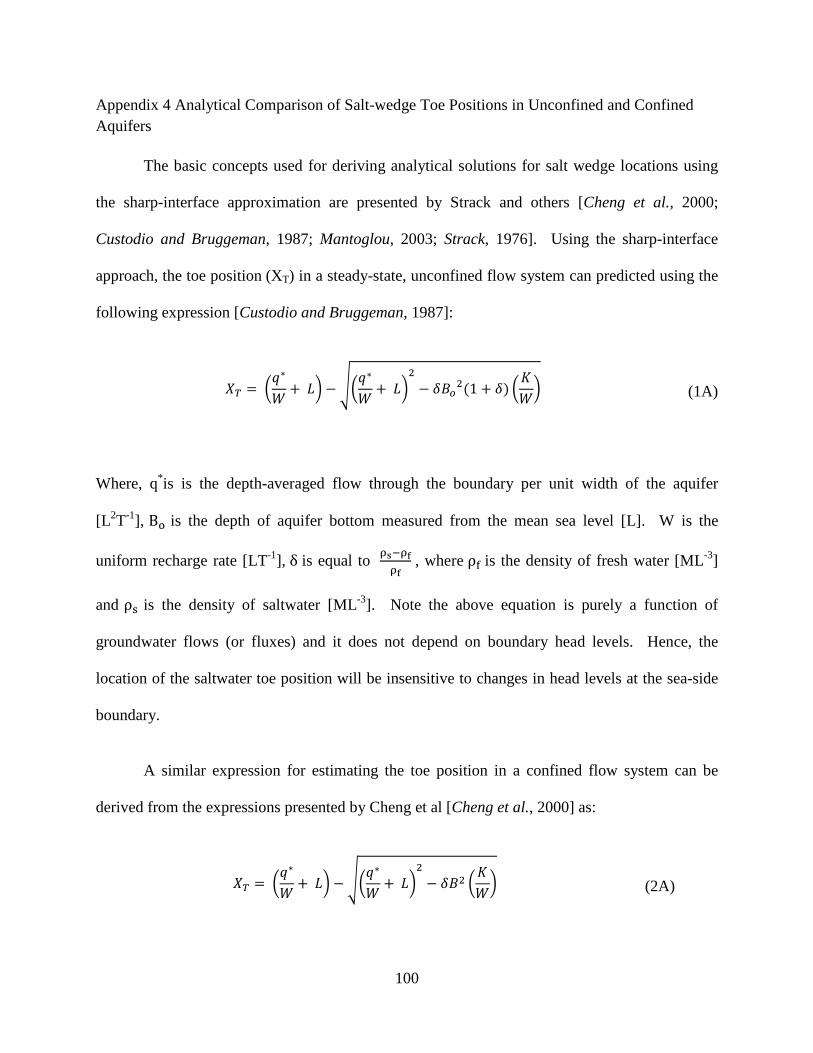
100
Appendix 4 Analytical Comparison of Salt-wedge Toe Positions in Unconfined and Confined Aquifers
The basic concepts used for deriving analytical solutions for salt wedge locations using
the sharp-interface approximation are presented by Strack and others [Cheng et al., 2000;
Custodio and Bruggeman, 1987; Mantoglou, 2003; Strack, 1976]. Using the sharp-interface
approach, the toe position (XT) in a steady-state, unconfined flow system can predicted using the
following expression [Custodio and Bruggeman, 1987]:
�� � ���� � �� � ���� � ��! � "#$!%1 � "' �(�� (1A)
Where, q* is is the depth-averaged flow through the boundary per unit width of the aquifer
[L2T-1], B) is the depth of aquifer bottom measured from the mean sea level [L]. W is the
uniform recharge rate [LT-1], δ is equal to +,�+-+- , where ρ is the density of fresh water [ML-3]
and ρ� is the density of saltwater [ML-3]. Note the above equation is purely a function of
groundwater flows (or fluxes) and it does not depend on boundary head levels. Hence, the
location of the saltwater toe position will be insensitive to changes in head levels at the sea-side
boundary.
A similar expression for estimating the toe position in a confined flow system can be
derived from the expressions presented by Cheng et al [Cheng et al., 2000] as:
�� � ���� � �� � ���� � ��! � "#! �(�� (2A)

101
Where, B is the thickness of the confined aquifer [L]. Equation (2A) is similar to (1A) and the
only difference is the (1 � δ' term. For seawater, the value of the dimensionless parameter δ =
0.025, and hence the term (1 � δ' ~ 1 . Therefore, when B!K~ B)!K (or when aquifer
thicknesses are matched approximately) the XT values predicted for confined and unconfined
flow systems would almost be the same.

102
Appendix 5 Derivation of Dimensionless Parameters for the Henry Problem and Analysis of
Henry-type Problem with Areal-recharge flux and zero regional flux
Notations
a = 0 +123%+,� +1' b = D/Q
ξ = l/d, aspect latio.
c = concentration of salt, in mass per unit volume of solution [ML-3].
cs = concentration of salt in sea water [ML-3].
Q = net fresh-water discharge per unit length of beach [L2].
u = horizontal velocity [LT-1].
v = vertical velocity [LT-1].
ρ = density of solution [ML-3].
ρo= density of freshwater [ML-3].
ρs= density of saltwater [ML-3].
φ’= dimensionless stream function
k = permeability of sand [L2].
d = thickness of aquifer [L].
l = length of aquifer [L].
P = fluid pore pressure [ML-1T-2].
g= acceleration of gravity [LT-2]
µ = viscosity of freshwater [ML-1T -1].
��$ = flux at the coastline or left boundary [L2T-1].
N = recharge rate [LT-1].

103
1. Dimensionless parameter of Henry Problem with regional flux
Scalar form of Darcy’s law can be written as:
�6 � 7 � �89 %:;:<' 1)
�= � > � �89 %:;:? � @A' 2)
Stream function definition in dimensionless form
7′ � :B′:? ′ > ′ � �:B′:< ′
C!B′ � ::< ′ D:B′
:< ′E � ::? ′ D:B′
:? ′E � :7′
:< ′ � :>′
:< ′ 3)
From the dimensionless form
7′ � FGH� > ′ � IGH� < ′ � 6G, ? ′ � =G, J ′ � KKL, @′ � M�MNML�MN Dimensionless derivation
:<:< ′ � O
:?:? ′ � O
:7′:? ′ � : :? ′ �7O�� � � O�� :7:? :?:? ′ � O!�� :7:?
:> ′:< ′ � : :< ′ �>O��� � O�� :>:< :<:< ′ � O!�� :>:<
:P ′:< ′ � : :< ′ �PPQ� � 1PQ :P:< :<:< ′ � OPQ :P:<

104
:@′:< ′ � : :< ′ � @ � @$@Q � @$� � 1@Q � @$ :@:< :<:< ′ � O@Q � @$ :@:<
Using these dimensionless form
Equation (3) is converted into dimensioned form
C!B′ � :7′:< ′ � :>′
:< ′ � O!�� :7:? � O
!�� :>:< � O
!�� % :7:? � :>:<'
RFR=, RIR6 terms are transformed in terms of pressure,
:7:? � : :? S�89 �:;:<�T � 89 :;:<:?
5)
:>:< � ::< S�89 �:;:? � @A�T � 89 :;:<:? � 8A9 :@:< 6)
When Subtract between equation (6) from (5) is
:7:? � :>:< � A :@:<
Therefore
C!B′ � O!�� � :7:? � :>:<� � O!�� � 8A9 :@:<� � O
!�� D9U(9@$ @Q � @$O :@′:< ′E � (O%@Q � @$'�� :J ′:< ′
using
( � 8@$A 9U
:@:< � @Q � @$O :@′:< ′ :@′:< ′ � :J′
:< ′

105
2. Dimensionless parameter of Henry Problem with areal-recharge flux �� � ��$ � V< � W%<'
:��:< � �V
From the dimensionless form
7′ � FGH�N�X6 > ′ � IGH�N�X6 < ′ � 6G, ? ′ � =G, J ′ � KKL, @′ � M�MNML�MN
Dimensionless derivation
:<:< ′ � O
:?:? ′ � O
:7′:? ′ � : :? ′ �7O�� � � O�� :7:? :?:? ′ � O!�� :7:?
:> ′:< ′ � : :< ′ �>O��� � O D� >��! :��
:< :<:< ′ � 1�� :>:< :<:< ′E � O D� >��! %�V'O � 1�� :>:< OE � O!��! %V> � �� :>:<'
:P ′:< ′ � : :< ′ �PPQ� � 1PQ :P:< :<:< ′ � OPQ :P:<
:@′:< ′ � : :< ′ � @ � @$@Q � @$� � 1@Q � @$ :@:< :<:< ′ � O@Q � @$ :@:<
Equation (3) is converted into dimensioned form
C!B′ � :7′:< ′ � :>′
:< ′ � O!�� :7:? � O
!��! �V> � �� :>:<� � O
!�� � :7:? � :>:<� � O
!��!V>
Due to the presence of the last term, which has dimensions, we were unable to cast this
problem in a fully non-dimensional form. Further analysis is needed to study this problem.

106
Appendix 6 Development of Two-dimensional Numerical Code for Simulating Saltwater Transport in Groundwater Systems
A7.1.Introduction
In the published literature, several numerical codes are available for simulating density-
coupled flow problems. The most commonly used codes are: SEAWAT [Guo and Langevin,
2002] which is based on a finite-difference formulation and FEFLOW [Diersch, 2002] and
SUTRA [Voss and Provost, 2002] which are based on a finite-element formulation. The source
code for SEAWAT uses a modified version of the USGS groundwater model MODFLOW to
simulate equivalent freshwater head as the principal dependent variable. In addition, it uses the
popular solution transport code MT3DMS to simulate salt and other solute transport processes.
Despite the availability of these public-domain/commercial codes, many researchers have
pointed out the need for more robust density coupled flow and transport models to study more
complex problems (e.g. metal leachate migration, transport of zero-valent iron, and redox
controlled dense metal plume transport, to name a few) [Goswami et al., 2012; Oostrom et al.,
1992; Schincariol and Schwartz, 1990]. Goswami et al. [2012], for example, has shown that
there are still several inaccuracies in simulating certain variable-density systems and hence more
research is needed to formulate computationally efficient codes to solve these systems.
Henry problem and Elder problem are commonly used benchmark problems for verifying
density-dependent groundwater codes. Simpson and Clement [2003] studied these two
benchmark problems using a coupled and uncoupled approach. The test showed that the Elder
problem is better than the Henry problem for testing variable-density codes.

107
The Henry problem, however, is the only variable density problem that has a semi-
analytical solution [Henry, 1964]. Henry used an analytical framework to define the location
and shape of the interface under a constant seaward freshwater flow moving toward an oceanic
boundary. Since Henry’s initial effort, several other analytical and numerical solutions have
been developed for the original Henry problem by Pinder and Cooper [1970], Lee and Cheng
[1974], Segol et al. [1975], Frind [1982], Huyakorn et al.[1987], and Voss and Souza [1987].
These studies have tested and modified some of the original parameters to fit Henry’s solution;
Croucher and O’sullivan [1995], reviewed all these studies and concluded that Henry’s original
analytical solution might have a minor error. Segol [1994] reinvestigated the errors associated
with the Henry solution and suggested some corrections. Simpson and Clement [2004]
developed an improved Henry problem. Goswami and Clement [2007] completed experimental
studies to develop a new benchmark dataset and used the coupled-uncoupled analysis to test the
worthiness of the new experimental problem for testing density-coupling effects. The results of
the analysis showed that the proposed experimental benchmark problem is a more robust
alternative to the traditional Henry problem.
The objective of the present work is to develop a computationally efficient finite-
difference algorithm that can solve a wide variety of two-dimensional, density-dependent flow
problems in saturated groundwater systems. The code was then tested using several benchmark
problems discussed in the previous section. The numerical code is built in Microsoft Excel
based Visual Basic framework. The finite-difference MODFLOW-family variable density flow
code SEAWAT [Guo and Langevin, 2002] was also used to simulate the benchmark datasets.
The model uses the pressure-based, finite-difference approach for formulating the governing
flow equations. The pressure based approach is relatively simple and direct compared to other

108
head-based formulations. For solving the solute transport, the advection process was solved
using the third-order TVD scheme and the dispersion/source terms are solved using implicit
finite-difference scheme.
A7.2 Governing Equation
The governing equations for density-dependent saturated flow through a two-dimensional
homogeneous and isotropic porous medium can be expressed as:
∂∂x SKg �∂P∂x �T � ∂∂z SKg �∂P∂z � ρg �T � ρS] ∂P∂t � θE∂C∂t (A7.1)
where, Sp [M-1LT2]is the specific storage in terms of pressure a� b,+-cd , P [ML-1T-2]is
pressure, ρ [ML -3]is the fluid density, θ is the water content, K [LT-1]is the hydraulic
conductivity, t [T] is time and x and z are the Cartesian coordinates, E is the density
concentration slope. The first term in the right-hand side of equation (A7.1) represents the rate
of fluid mass accumulation due to ground-water storage effects (for example, due to the
compressibility of the bulk porous material and fluid compressibility). The second term in the
right-hand side of the equation represents the rate of fluid mass accumulation due to the change
of solute concentration.
The two-dimensional transport is modeled using the advection-dispersion equation,
which is solved using the operator split strategy. The governing equation and the operator split
version of the transport equations can be written as:
∂C∂t � �Ve ∂C∂x � Vf ∂C∂y � ∂∂x %De ∂C∂x' � ∂∂y %Df ∂C∂y' (A7.2)

109
∂C ∂t � �Ve ∂C
∂x � Vf ∂C
∂y
(A7.2a)
∂Ci∂t � ∂∂x %De ∂Ci∂x' � ∂∂y %Df ∂Ci∂y' (A75.2b)
where, Ve and Vf�L/T� are velocity, C [ML-3] is the solute concentration, De and Df [L2/T] are
are the hydrodynamic dispersion coefficient.
In the operation split method, the advection part of the equation is solved as shown in equation %A7.2a' using TVD package. Subsequently, the concentration obtained from advection %Ci' is used to solve the dispersion part of the equation as shown in equation %A7.2b' using Implicit FDM. To calculate velocity at nodes, the specific discharge is divided by
porosity. The general expression for specific discharge (Darcy flux) can be written as: qe � �keµ ∂P∂x (
q� � �k�µ %∂P∂z � ρg ' (A7.3)
where qe and qe are the individual component of specific discharge, P is pressure [ML-1T-2], ρ is
the fluid density [ML-3], g is acceleration due to gravity [LT-2].
Equation %A7.1' and %A7.2' are coupled through equation %A7.4'. ρ � ρ � EC (A7.4)

110
Based on SI unit, the value of typical seawater concentration is about 35 kg/m3 and the
freshwater density is set to 1,000 kg/m3 and saltwater density is set to 1,025 kg/m3 with the
density slope of 0.714 (� 3�����f 3�������, !� 2c/��b�������� �)���������)�, �� 2c/��). A7.3 Model Development
Flow Equation
∂∂x SKg �∂P∂x �T � ∂∂z SKg �∂P∂z � ρg �T (A7.5a)
� Kg∆x � DP���,��,� � P�,��,�∆x E � DP�,��,� � P���,��,�∆x E�� Kg∆y � DP�,���
�,� � P�,��,�∆y E � DP�,��,� � P�,����,�∆y E�� K g∆y Sρ���!,����,�g � ρ���!,����,�gT
where n denotes the nth discrete time level, tn, when the solution is known, and m is the Picard
iteration level, P�,� is the pressure head at node ij . The subscripts i+1/2, i-1/2 refer to the value
between two neighboring cells. The density between two cells expressed as average value. The
nodal order matches the numbering order of VBA language for all formulation in this study.
The current and previous iteration levels are denoted as m and m-1, respectively.
ρS] ∂P∂t � θE∂C∂t � ρ�,�S] P�,��,� � P�,� ���∆t � θEC�,����,� � C�,����∆t (A7.5b)
where, ∆t � t� � t��� is the time step, which in general is set to maintain acceptably small
temporal variation in pressure head.
The finite difference form reduced to

111
a1 P���,��,� � b1 P�,����,� � c1 P�,��,� � d1 P�,����,� � e1 P���,��,� � RHS %A7.6' where,
a1 � � Keg∆x! b2 � � K�g∆z!
c1 � 2 � K�g∆x! � K�g∆z!� � ρ�,� S]∆t d1 � � K�g∆z! e1 � � Keg∆x!
RHS � K�2∆z �ρ���,����,� � ρ���,����,�� � ρ�,� S]∆t P�,� ��� � θE∆t %C�,����,� � C�,����' Eq. (A7.6) applies to all interior nodes: at boundary nodes this equation is modified to
reflect the appropriate boundary conditions. This would lead to a system of linear equations of
the form:
A · P� � b %A7.7' Where, A is a banded square matrix, P� is the vector of unknown pressure at the current time level
n and iteration level, m, and b is the forcing vector. The set of linear algebraic equations are
solved using a banded version of a Gauss–elimination solver.
Transport Equation
The linear formulation for TVD scheme for advection package is described below. Equation %A7.7a' is spatial formulation and equation %A7.7b' is temporal formulation.

112
�Ve ∂C∂x � Vf ∂C∂y� �V�,���/!C�,���/!� � V�,���/!C�,���/!�
Δy � V���/!,�C���/!,�� � V���/!,�C���/!,��Δx
%A7.7a'
∂C ∂t � C�,���� � C�,��Δt %A7.7b'
The TVD scheme adopts a universal flux limiting procedure to minimize numerical oscillations
which may occur if sharp concentration fronts are involved. This scheme is mass conservative,
without excessive numerical dispersion, and essentially oscillation-free. Appendix 8 illustrates
the detailed TVD formulation procedure and the application of universal limiter.
The implicit FDM formulation is described below for dispersion package. Equation %A7.8a' is spatial formulation and equation %A7.8b' is temporal formulation. � ∂∂x %De ∂C∂x' � ∂∂y %Df ∂C∂y'
� 1 ∆x £ D���!,� ���,� DC���,��,� � C�,��,�∆x E � D���!,�
���,� DC�,��,� � C���, j�,�∆x E¥� 1 ∆x £ D�,���!
���,� DC�,��,� � C�,����,�∆x E � D�,���! ���,� DC�,��,� � C�,����,�∆x E¥
%A7.8a'
∂C ∂t � C�,���� � C�,��Δt
%A7.8b' Note that the average dispersion tensor used in the spatial terms is the value that was updated by
the previous iteration step, m-1. The value is calculated explicitly so that the equation has only
concentration as an independent variable to solve in linear matrix.
The general expression for finite difference form is
a!C���,��,� � b! C�,����,� � c! C�,��,� � d! C�,����,� � e! C���,��,� � RHS (A7.9)

113
where,
a! � De���!,� ���,� 1 ∆x!
b! � Df�,���! ���,� 1 ∆y!
c! � � 1 ∆x! DDe���!,� ���,� � De���!,�
���,�E � 1 ∆y! DDf�,���! ���,� � Df�,���!
���,�E � 1 d! � Df�,���!
���,� 1 ∆y! e! � De���!,�
���,� 1 ∆x! RHS � C��,��,�∆t
Eq. (A7.9) applies to all interior nodes: at boundary nodes this equation is modified to reflect the
appropriate boundary conditions. The resulting system of linear equations is also solved by the
banded Gauss-elimination solver.
Boundary Conditions
Test problems-1, 2 and 4 use Dirichlet boundary condition for freshwater boundary. Test
problem-3 uses Numann boundary condition for freshwater inflow. Also, the tank bottom is set
to no-flow boundary for all test problems. Saltwater intrusion modifies the concentration at the
boundary. The detailed modification is expressed in the model setup for each test problem.
Time Step Determination
Since advection is solved by explicitly, Courant condition is required to limit transport
time step, ∆t. Courant condition is applied to all simulations to maintain sufficiently small time
steps. The length of time step is calculated by Courant condition to satisfy the stability

114
constraints and accuracy requirements of the transport equation. In this study, saltwater
simulation generally set the Courant number to 0.5. The Elder problem decreases the Courant
number to 0.1.

115
A7.3 Results
Test Problem 1: Sinking plume model
The first test problem is an example of dense solute transport. Goswami et al. [2012]
provided an experimental and numerical solution conducted in a two-dimensional flow tank
using three different numerical techniques available in SEAWAT/MT3DMS. The experiments
were designed to represent a sinking groundwater plume and a rising groundwater plume. This
problem is also helpful when applied to practical environmental issues such as contaminant
transport and tsunami issues in coastal aquifers. The domain and boundary conditions describe a
confined aquifer; constant freshwater pressure heads are maintained on the left and the right
boundary of the main, respectively (see Figure A7.1). The two-dimensional modeling domain is
225 mm long and 180 mm high. The longitudinal dispersivity value was set to 0.1 mm and
transverse dispersivity is set to 0.01 mm. Three stress periods were employed to simulate the
following three experimental stages: (1) steady-state conditions prior to injection, (2) injection of
freshwater/saltwater slug, and (3) migration of slug through the tank. The time step size was set
to an initial minimum value of 0.1 s and a maximum value of 1 s. The Courant number constraint
was set to 0.5. Values for this model are presented in Table A7.1.
The simulated results of third state (migration stage) were compared to SEAWAT results
and shown in Figure A7.2. The simulation shows good agreement with SEAWAT (See Figure
A7.4). The density-dependent sinking study can be also applied to a different composition in
fluid from typical seawater or the salt concentration. For example, Kanel et al. [2008] simulated
the fate and transport of Zero-valent iron nanoparticles (INP) and stabilized zero-valent iron
nanoparticles using poly acrylic acid (S-INP) in porous media under saturated, steady-state flow
conditions.

116
Figure A7.1 Conceptual description of the numerical model used for simulating the sinking-
plume experiments (Goswami et al, 2012).
Table A7.1 Summary of numerical model parameters
Property Symbol values
Horizontal length L 23 cm
Vertical Length hs 18 cm
Hydraulic conductivity K 1.16 cm/s
Porosity n 0.38
Specific storage, Ss 0.000001cm-1
Longitudinal dispersivity αL 0.01 cm
Transverse dispersivity αT 0.001 cm
Saltwater concentration Cs 0.035 g/cm3
Saltwater density ρs 1.025 g/cm3
Freshwater density ρf 1.000 g/cm3
Density slope E 0.714

117
(a) VDFT code (b) SEAWAT
Figure A7.2 Comparison of VDFT code simulation results against to SEAWAT for the sinking
plume experiment at various times at 0 min (left plume) , 2 min (middle) and 4 min (right),
Red color > 10% and Blue color 1 – 10 % .
0 5 10 15 200
2
4
6
8
10
12
14
16
18
0 5 10 15 200
2
4
6
8
10
12
14
16
18

118
Test Problem 2: Saltwater Intrusion Model
A conceptual model based on Goswami and Clement [2007] was simulated. The
saltwater behavior in the saltwater intrusion problem is relatively stable. Goswami and Clement
[2007] proposed the experimental data set that can be used as a benchmark problem. The
domain and boundary conditions describe a confined aquifer; constant pressure heads are
maintained on the left and the right boundary of the main, respectively (see Figure A7.3). This
Henry-type problem is useful to understand the role of several hydrodynamic and geologic
factors affecting the flow and transport process in the simplified flow system. In order to
construct the numerical model, the origin of an x-z coordinate system was set on the lower left-
hand corner of the plane. A uniform grid of size 1.0 cm (54 cells in the x-direction and 26 cells
in the z-direction) was used to discretize the 53.0 cm × 26.0 cm dimensional model. The
saltwater head is imposed on left boundary where the head is set to 25.5 cm for the entire
simulation time. The value of specific storage (Ss) was set to 10-6 cm-1 for all nodes. All layers
are set to confined layer and bottom of the model is set to no-flow condition. Freshwater flux is
allowed to penetrate from the right constant-head boundary. The value of 0.05 cm and 0.005 cm
were selected for the longitudinal and transversal dispersivity coefficient, respectively. Values
for this model are presented in Table A7.2.
Three steady state conditions were selected and simulated using VDFT code and
compared to SEAWAT results. The simulation shows good agreement with SEAWAT for the
steady-state condition (See Figure A7.4). Transient simulations for an intruding condition and a
receding condition also show good agreements (See Figure A7.5).

119
Figure A7.3 Computation domain and boundary conditions used in the numerical model
(Goswami and Clement, 2007)
Table A7.2 Summary of numerical model parameters
Property Symbol values
Horizontal length L 53 cm
Saltwater elevation hs 26 cm
Hydraulic conductivity K 1.215 cm/s
Porosity n 0.385
Specific storage, Ss 0.000001cm-1
Longitudinal dispersivity αL 0.01 cm
Transverse dispersivity αT 0.001 cm
Saltwater concentration Cs 0.0371 g/cm3
Saltwater density ρs 1.026 g/cm3
Freshwater density ρf 1.000 g/cm3
Density Slope E 0.714

120
Figure A7.4 Comparison of VDFT code simulation results against to SEAWAT for steady state
in saltwater problem.
0
5
10
15
20
25
0 10 20 30 40 50
z (c
m)
x (cm)
VDFT SS1VDFT SS2VDFT SS3SEAWAT

121
(a)
(b)
Figure A7.5 Comparison of VDFT code simulation results against to SEAWAT for (a) intruding
and (b) receding condition in saltwater problem.
0
5
10
15
20
25
0 10 20 30 40 50
z (c
m)
x (cm)
VDFT 5 minutesVDFT 15 minutesVDFT 55 minutesSEAWAT
0
5
10
15
20
25
0 10 20 30 40 50
z (c
m)
x (cm)
VDFT10 minutesVDFT 15 minutesVDFT 25 minutesSEAWAT

122
Test Problem 3: Flux-type Henry Problem
Conceptual models based on original Henry problem [1964] and modified Henry
problem [Simpson and Clement, 2004] were simulated. The domain and boundary conditions for
the Henry and Modified Henry problem describe a confined aquifer. A constant pressure head is
maintained on the right boundary and constant flux is maintained on the left boundary of the
main (see Figure A7.6). In order to construct a numerical model, the origin of an x-z coordinate
system was set on the lower left-hand corner of the plane. A uniform grid of size 5.0 cm (41
cells in the x-direction and 20 cells in the z-direction) was used to discretize the 200 cm × 100
cm dimensional model. The saltwater head is imposed on the right boundary where the head is
set to 100 cm for the entire simulation time. The value of specific storage (Ss) was set to 10-6 cm-
1 for all nodes. All layers are set to confined layer and bottom of the model is set to no-flow
condition. The longitudinal and transversal dispersivity coefficients are set to zero. Values for
this model are presented in Table A7.3.
The simulated results for (a) original Henry problem and (b) modified Henry problem
were compared to SEAWAT results and shown in Figure A7.7. This difference indicates that the
relative importance of the density effects is greater for the modified case where the influence of
the boundary forcing is reduced [Simpson and Clement, 2004]. In this figure, bigger discrepancy
is shown at the bottom of the model when the modified Henry problem was simulated. The
VDFT code is still under development to predict more accurate density effects.

123
Figure A7. 6 Boundary conditions applied for solving Henry saltwater intrusion Problem (Henry,
1964; Simpson and Clement, 2003).
Table A7.3 Summary of numerical model parameters
Property Symbol values
Horizontal length L 200 cm
Saltwater elevation hs 100 m
Freshwater darcy flow q 6.6 × 10⁻³ cm/s
Hydraulic conductivity K 1.0 cm/s
Porosity n 0.35
Specific storage, Ss 0 cm-1
Longitudinal dispersivity αL 0 cm
Transverse dispersivity αT 0 cm
Saltwater concentration Cs 35 kg/m3
Saltwater density ρs 1,025 kg/m3
Freshwater density ρf 1,000 kg/m3
Density slope E 0.714
Diffusion coefficient Dm 1.886 × 10⁻⁵ cm2/s
0
20
40
60
80
100
0 20 40 60 80 100 120 140 160 180 200
Ele
vatio
n (
cm)
Length (cm)
¦§ � ¨. ¨ × ª« �¨ ¬ �ª %®¯°±² ³±´µ¶¯¬' � ·. · × ª« �¨ ¬ �ª %¸´¹º»º¯¹ ®¯°±² ³±´µ¶¯¬' ¼ � «
¦½ � «, ¾¼¾½ � «
¦½ � «, ¾¼¾½ � « ¿ � ÀÁ ÃÁ ¼ � ¼Á ÄŠƧ < «
¾¼¾§ � « ÄŠƧ ≥ «

124
Figure A7.7. Steady-state 50% isochlor distribution for the Henry Problem and the modified
Henry problem.
0
20
40
60
80
100
0 20 40 60 80 100 120 140 160 180 200
z (c
m)
x (cm)
VDFT - Modified Henry problem (2004)VDFT - Henry problem (1964)SEAWAT

125
Test Problem 4: Elder Problem
A conceptual model based on original Elder Problem [Elder, 1967] was simulated. This
study follow the aquifer property and parameter values suggested by Simpson and Clement
[2003]. The domain and boundary conditions for the Elder problem describe a confined aquifer,
a zero pressure head is maintained on the left and right upper corner of the domain (see Figure
A7.8). In order to construct a numerical model, the origin of an x-z coordinate system was set on
the lower left-hand corner of the plane. A grid of size of 16.8 m for x-direction and 6 m of z-
direction (44 cells in the x-direction and 25 cells in the z-direction) was used to discretize the
600 m × 150 m dimensional model. The value of specific storage (Ss) was set to zero for all
nodes. All layers are set to confined layer and bottom of the model is set to no-flow condition.
The longitudinal and transversal dispersivity coefficients are set to zero. Cells in layer 1 from
columns 12 to 33 are imposed by constant concentration with a value of 285.7 kg/m3. The
Courant number is set to 0.1. The model summary is presented in Table A7.3.
The simulated results were compared to SEAWAT results and shown in Figure A7.9.
VDFT results show relatively smooth migration downward where SEAWAT shows clear
vortices in the model. The VDFT code is still under development to predict more accurate
density effects.

126
Figure A7.8. Domain and boundary conditions for the Elder problem (Simpson and Clement, 2003).
Table A7.4 Summary of numerical model parameters
Property Symbol values
Horizontal length L 600 m
Saltwater elevation hs 150 m
Hydraulic conductivity K 4.76 × 10⁻⁶ cm/s
Porosity n 0.1
Specific storage, Ss 0 cm-1
Longitudinal dispersivity αL 0 cm
Transverse dispersivity αT 0 cm
Saltwater concentration Cs 286 kg/m3
Saltwater density ρs 1,200 kg/m3
Freshwater density ρf 1,000 kg/m3
Density Slope E 0.7
Diffusion coefficient Dm 3.57 × 10⁻⁶ cm2/s

127
(a) 2 years at SEAWAT (b) 2 years at VDFT
(c) 4 years at SEAWAT (d) 4 years at VDFT
Figure A7.9. 20% (blue line) and 60% (red line) of the flow pattern of the dense fluid into the
aquifer for the Elder Problem.
A7.4 Discussion
The VDFT code currently reproduces the experiment data well; however, some discrepancies
where observed for certain benchmark problems (Henry problem and Elder problem). The
implicit transport package of VDFT code is still under development, and further work is needed
to improve this package.
0 100 200 300 400 500 6000
50
100
150
0 100 200 300 400 500 6000
50
100
150
0 100 200 300 400 500 6000
50
100
150
0 100 200 300 400 500 6000
50
100
150

128
Appendix 7 Code Formulation based on TVD Scheme for Advection Package
1. General Formulation (assume constant ɧ) θ C�,���� � C�,��Δt � �q�,���/!C�,���/!� � q�,���/!C�,���/!�
Δy � q���/!,�C���/!,�� � q���/!,�C���/!,��Δx
Rearranging terms
C�,���� � C�,�� � %γ'��cË�C�,���/!� � %γ'���C�,���/!� � %γ'Ì)��)�C���/!,�� � %γ'�)]C���/!,��
Where the Courant number, γ, is defined as
%γ'��� � q�,���/!ΔtθΔx � ve�,���/!Δt Δx %γ'��cË� � q�,���/!ΔtθΔx � ve�,���/!Δt Δx %γ'�)] � q���/!,�ΔtθΔy � vf���/!,�Δt Δy %γ'Ì)��)� � q���/!,�ΔtθΔy � vf���/!,�Δt Δy
Applying the same procedure for third-order polynomial interpolation of nodel
concentrations as described in chapter 3 (MT3DMS manual), the concentration values at the left
interface can be derived as
C�,���/!� � Ci�,���/!� � de2 fe � df2 ff � ÍΔy! � df!Î6 fff � Dde!6 � Δxde4 E fee � Ddedf3 � Δyde4 E ffe
Where,
df � ve�,���/!Δt de � vf�,���/!Δt

129
Ci �,���/!� � C�,���� � C�,�� 2 , in this study
The normal gradient
ff � C�,�� � C�,���� Δy
The upwind gradient along the y-direction depends on the directions of the velocities
fe � ÍC�,���� � C���,���� Î/Δx vf�,���/! Ð 0, ve �,���/! Ð 0 � ÍC���,���� � C�,���� Î/Δx vf�,���/! Ð 0, ve �,���/! < 0 � ÍC�,�� � C���,�� Î/Δx vf�,���/! < 0, ve �,���/! Ð 0 � ÍC���,�� � C�,�� Î/Δx vf�,���/! < 0, ve �,���/! < 0
Based on the first-order derivatives,
Second order derivatives can be calculated below:
fff � SÍffÎ�,���! � ÍffÎ�,�����!T /Δy vf�,���/! Ð 0
� SÍffÎ�,���! � ÍffÎ�,���!T /Δy vf�,���/! < 0
fee � S%fe'���!,��� � %fe'���!,���T /Δy vf�,���/! Ð 0
� S%fe'���!,� � %fe'���!,�T /Δy vf�,���/! < 0
Mixed second-order derivatives (twist terms)
ffe � S%fe'���!,� � %fe'���!,���T /Δy ve�,���/! Ð 0
� S%fe'���!,� � %fe'���!,���T /Δy ve�,���/! < 0
C���/!,��
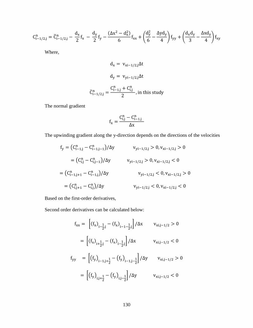
130
C���/!,�� � Ci ���/!,�� � de2 fe � df2 ff � %Δx! � de!'6 fee � Ddf!6 � Δydf4 E fff � Ddedf3 � Δxdf4 E fef
Where,
de � ve���/!,�Δt df � vf���/!,�Δt
Ci ���/!,�� � C���,�� � C�,�� 2 , in this study The normal gradient
fe � C�,�� � C���,�� Δx
The upwinding gradient along the y-direction depends on the directions of the velocities
ff � ÍC���,�� � C���,���� Î/Δy vf���/!,� Ð 0, ve���/!,� Ð 0 � ÍC�,�� � C�,���� Î/Δy vf���/!,� Ð 0, ve���/!,� < 0
� ÍC���,���� � C���,�� Î/Δy vf���/!,� < 0, ve���/!,� Ð 0 � ÍC�,���� � C�,�� Î/Δy vf���/!,� < 0, ve���/!,� < 0
Based on the first-order derivatives,
Second order derivatives can be calculated below:
fee � S%fe'���!,� � %fe'�����!,�T /Δx ve�,���/! Ð 0
� S%fe'���!,� � %fe'���!,�T /Δx ve�,���/! < 0
fff � SÍffÎ���,���! � ÍffÎ���,���!T /Δy ve�,���/! Ð 0
� SÍffÎ�,���! � ÍffÎ�,���!T /Δy ve�,���/! < 0

131
Mixed second-order derivatives (twist terms)
fef � SÍffÎ�,���! � ÍffÎ���,���!T /Δx vf���/!,� Ð 0
� SÍffÎ� ,���! � ÍffÎ���,���!T /Δx vf���/!,� < 0
2. Limiter Application
CÒ � C � C��!C� � C��! Note that
CÒ ��! � 0 and CÒ � � 1 If the concentration profile across the three nodes are monotonic,
CÒ ��� Ó CÒ ���! Ó 1
Which equal to
C��� � C��!C� � C��! Ó C���! � C��!C� � C��! Ó 1
C��� � C��! Ó C���! � C��! Ó C� � C��! The right-hand inequality in above equation is insured
C���! Ó C� constraint %1' The left-hand inequality in above equation is insured
C���! ≥ C��� constraint %2'
Also, Explicit finite difference solution at note j-1 is

132
C������ � C���� � Cr %C���!� � C�����!� ' Is transformed in terms of normalized variables,
CÒ ������ � CÒ ���� � Cr %CÒ ���!� � CÒ �����!� ' Since
CÒ ���!� ≥ CÒ �����!� due to monotonic 0 Ó CÒ ������ Ó CÒ ���� Ó 1
Left-hand inequality implies
0 Ó CÒ ������ 0 Ó CÒ ���� � C� %CÒ ���!� � CÒ �����!� ' CÒ ���!� Ó CÒ �����!� � CÒ ���� /C�
The worst –case estimate for CÒ ����ÔÕ� � 0 results in additional constraints on CÒ ��ÔÕ� :
CÒ ���!� Ó CÒ ���� /C� JÖ×ØÙÚÛÙÜ×Ù %3'
If CÒ ��ÔÕ� does not lie with above boundary,
CÒ ���!� � CÒ ����
Therefore
C���!� � C����

133
References
Abarca, E., and T. P. Clement (2009), A novel approach for characterizing the mixing zone of a saltwater wedge, Geophysical Research Letters, 36(6).
Abarca, E., J. Carrera, X. Sánchez-Vila, and C. I. Voss (2007a), Quasi-horizontal circulation cells in 3D seawater intrusion, Journal of Hydrology, 339(3-4), 118-129.
Abarca, E., J. Carrera, X. Sánchez-Vila, and M. Dentz (2007b), Anisotropic dispersive Henry problem, Advances in Water Resources, 30(4), 913-926.
Anderson, J., K. Milliken, D. Wallace, A. Rodriguez, and A. Simms (2010), Coastal Impact Underestimated From Rapid Sea Level Rise, Eos Trans. AGU, 91(23), 205-206, doi: 10.1029/2010EO230001
Barlow, P. M., and E. G. Reichard (2010), Saltwater intrusion in coastal regions of North America, Hydrogeology Journal, 18(1), 247-260.
Bear, J., and A. H. D. Cheng (2010), Modeling groundwater flow and contaminant transport, 1st edition ed., Springer.
Blanchon, P., A. Eisenhauer, J. Fietzke, and V. Liebetrau (2009), Rapid sea-level rise and reef back-stepping at the close of the last interglacial highstand, Nature, 458(7240), 881-884.
Boufadel, M. C. (2000), A mechanistic study of nonlinear solute transport in a groundwater-surface water system under steady state and transient hydraulic conditions, Water Resour. Res., 36(9), 2549-2565.
Chang, S. W., and T. P. Clement (2012a), Laboratory and numerical investigation of transport processes occurring beneath a saltwater wedge Journal of Contaminant Hydrology, sumbitted.
Chang, S. W., and T. P. Clement (2012b), Experimental and numerical investigation of saltwater intrusion dynamics in flux controlled groundwater systems, Water Resources Research, doi:10.1029/2012WR012134, In press.
Chang, S. W., T. P. Clement, M. J. Simpson, and K.-K. Lee (2011), Does sea-level rise have an impact on saltwater intrusion?, Advances in Water Resources, 34(10), 1283-1291.
Cheng, A. H. D., D. Halhal, A. Naji, and D. Ouazar (2000), Pumping optimization in saltwater-intruded coastal aquifers, Water Resources Research, 36(8), 2155-2165.

134
Clement, T. P., Y. Sun, B. S. Hooker, and J. N. Petersen (1998), Modeling Multispecies Reactive Transport in Ground Water, Ground Water Monitoring & Remediation, 18(2), 79-92.
Croucher, A. E., and M. J. O'Sullivan (1995), The Henry Problem for Saltwater Intrusion, Water Resour. Res., 31(7), 1809-1814.
Custodio, E., and G. A. Bruggeman (1987), Groundwater problems in coastal areas. Studies and reports in hydrology 45, edited, UNESCO, Paris.
Dausman, A., and C. Langevin (2005), Movement of the saltwater interface in the Surficial Aquifer System in response to hydrologic stresses and water-management practices, Broward County, Florida: USGS Scientific Investigations Report : SIR 2004-5256Rep.
Destouni, G., and C. Prieto (2003), On the possibility for generic modeling of submarine groundwater discharge, Biogeochemistry, 66(1), 171-186.
Diersch, H. J. G. (2002), FEFLOW finite element subsurface flow and transport simulation system -user's manual/reference manual/whilte papers. Release 5.0Rep., Berlin.
Elder, J. W. (1967), Steady free convection in a porous medium heated from below, Journal of Fluid Mechanics, 27(01), 29-48.
Feseker, T. (2007), Numerical studies on saltwater intrusion in a coastal aquifer in northwestern Germany, Hydrogeology Journal, 15(2), 267-279.
Fetter, C. W. (2001), Applied Hydrogeology, Prentice Hall, N.J.
Frind, E. O. (1982), Simulation of long-term transient density-dependent transport in groundwater, Advances in Water Resources, 5(2), 73-88.
Giambastiani, B. M. S., M. Antonellini, G. H. P. Oude Essink, and R. J. Stuurman (2007), Saltwater intrusion in the unconfined coastal aquifer of Ravenna (Italy): A numerical model, Journal of Hydrology, 340(1-2), 91-104.
Goswami, R. R., and T. P. Clement (2007), Laboratory-scale investigation of saltwater intrusion dynamics, Water Resources Research, 43(4), doi: 10.1029/2006WR005151.
Goswami, R. R., B. Ambale, and T. P. Clement (2009), Estimating errors in concentration measurements obtained from image analysis, Vadose Zone Journal, 8(1), 108-118.
Goswami, R. R., T. P. Clement, and J. H. Hayworth (2012), Comparison of Numerical Techniques Used for Simulating Variable-Density Flow and Transport Experiments, Journal of Hydrologic Engineering, 17(2), 272-282.

135
Green, T. R., M. Taniguchi, H. Kooi, J. J. Gurdak, D. M. Allen, K. M. Hiscock, H. Treidel, and A. Aureli (2011), Beneath the surface of global change: Impacts of climate change on groundwater, Journal of Hydrology, 405(3-4), 532-560.
Guo, W., and C. D. Langevin (2002), User's Guide to SEWAT: A Computer Program for Simulation of Three-Dimensional Variable-Density Ground-Water Flow, United States Geological Survey.
Henry, H. R. (1964), Effects of dispersion on salt encroachment in coastal aquifers, U.S. Geological Survey Water-Supply Paper Rep. 1613-C, C71-C84. pp.
Huyakorn, P. S., P. F. Andersen, J. W. Mercer, and H. O. White, Jr. (1987), Saltwater intrusion in aquifers: Development and testing of a three-dimensional finite element model, Water Resour. Res., 23(2), 293-312.
Illangasekare, T., et al. (2006), Impacts of the 2004 tsunami on groundwater resources in Sri Lanka, Water Resour. Res., 42(5), W05201.
IPCC (2007), Climate change 2007: Impacts, adaptation and vulnerability, Contribution of Working Group II to the Fourth Assessment Report of the Intergovernmental Panel on Climate Change, edited by M. L. Parry, O. F. Canziani, J. P. Palutikof, P. J. van der Linden and C. E. Hanson, Cambridge University Press Cambridge.
Johannes, R. E. (1980), The ecological significance of the submarine discharge of groundwater, Marine Ecology Progress Series 3, 365–-373.
Kanel, S. R., R. R. Goswami, T. P. Clement, M. O. Barnett, and D. Zhao (2008), Two dimensional transport characteristics of surface stabilized zero-valent iron nanoparticles in porous media, Environ Sci Technol, 42(3), 896-900.
Karasaki, K., K. Ito, and K. Maekawa (2006), Simulation of salt water intruison, paper presented at TOUGH Symposium, Lawrence Berkeley National Laboratory, Berkely, California.
Kohout, F. A. (1960), Cyclic Flow of Salt Water in the Biscayne Aquifer of Southeastern Florida, J. Geophys. Res., 65(7), 2133-2141.
Kuan, W. K., G. Jin, P. Xin, C. Robinson, B. Gibbes, and L. Li (2012), Tidal influence on seawater intrusion in unconfined coastal aquifers, Water Resour. Res., 48(2), W02502.
Kundzewicz, Z. W., and P. Dölle (2009), Will groundwater ease freshwater stress under climate change?, Hydrological Sciences Journal, 54(4), 665-675.
Lacombe, P. J., and G. B. Carleton (1992), Saltwater intrusion into fresh ground-water supplies, southern Cape May County, New Jersey, 1890-1991.

136
Langevin C, Shoemaker WB, and G. W (2003), Modflow-2000, The USGS Geological Survey modular ground-water model – documentation of the Seawat-2000 version with the variable density flow process (VDF) and the integrated MT3DMS transport process (IMT)Rep., US Geological Survey.
Leatherman, S. P. (1984), Coastal geomorphic response to sea level rise : Galveston Bay, Texas, in Barth M.C., Titus J.G. (eds) Greenhouse effect and sea level rise : a challenge for this generation.Rep., 151-178 pp, Reinhold, New York.
Lee, C. H., and R. T. S. Cheng (1974), On seawater encroachment in coastal aquifers, Water Resources Research, 10, 1039-1043.
Li, H., and J. J. Jiao (2003a), Influence of the tide on the mean watertable in an unconfined, anisotropic, inhomogeneous coastal aquifer, Advances in Water Resources, 26(1), 9-16.
Li, H., and J. J. Jiao (2003b), Tide-induced seawater-groundwater circulation in a multi-layered coastal leaky aquifer system, Journal of Hydrology, 274(1-4), 211-224.
Li, H., M. C. Boufadel, and J. W. Weaver (2008), Tide-induced seawater-groundwater circulation in shallow beach aquifers, Journal of Hydrology, 352(1-2), 211-224.
Li, L., D. A. Barry, F. Stagnitti, and J. Y. Parlange (1999), Submarine groundwater discharge and associated chemical input to a coastal sea, Water Resour. Res., 35(11), 3253-3259.
Loáiciga, H. A., T. J. Pingel, and E. S. Garcia (2011), Sea Water Intrusion by Sea-Level Rise: Scenarios for the 21st Century, Ground Water, no-no.
Mantoglou, A. (2003), Pumping management of coastal aquifers using analytical models of saltwater intrusion, Water Resources Research, 39(12), 1335.
Masterson, J. P., and S. P. Garabedian (2007), Effects of Sea-Level Rise on Ground Water Flow in a Coastal Aquifer System, Ground Water, 45(2), 209-217.
McCarthy, J. J. (2009), Reflections On: Our Planet and Its Life, Origins, and Futures, Science, 326(5960), 1646, doi: 10.1126/science.1184937.
Meisler, H., Leahy PP and Knobel LL. (1985), The effect of eustatic sea-level changes on saltwaterfreshwater relations in the northern Atlantic Coastal Plain: U.S. Geological Survey Water-Supply Paper 2255, 28 p.Rep.
Melloul, A., and M. Collin (2006), Hydrogeological changes in coastal aquifers due to sea level rise, Ocean & Coastal Management, 49(5-6), 281-297.
Michael, H. A., A. E. Mulligan, and C. F. Harvey (2005), Seasonal oscillations in water exchange between aquifers and the coastal ocean, Nature, 436(7054), 1145-1148.

137
Moore, W. S. (1996), Large groundwater inputs to coastal waters revealed by 226Ra enrichments, Nature, 380(6575), 612-614.
Moore, W. S., and T. M. Church (1996), Submarine Groundwater Discharge, reply to Younger., Nature, 382, 122.
Navoy, A. S. (1991), Aquifer-estuary interaction and vulnerability of groundwater supplies to sea level rise-driven saltwater intrusion, Pennsylvania State University, USA.
Oostrom, M., J. S. Hayworth, J. H. Dane, and O. Güen (1992), Behavior of dense aqueous phase leachate plumes in homogeneous porous media, Water Resour. Res., 28(8), 2123-2134.
Oude Essink, G. H. P. (2001), Salt Water Intrusion in a Three-dimensional Groundwater System in The Netherlands: A Numerical Study, Transport in Porous Media, 43(1), 137-158.
Oude Essink, G. H. P., E. S. van Baaren, and P. G. B. de Louw (2010), Effects of climate change on coastal groundwater systems: A modeling study in the Netherlands, Water Resour. Res., 46, W00F04.
Pinder, G. F., and H. H. Cooper, Jr. (1970), A Numerical Technique for Calculating the Transient Position of the Saltwater Front, Water Resour. Res., 6(3), 875-882.
Ranjan, P., S. Kazama, and M. Sawamoto (2006), Effects of climate change on coastal fresh groundwater resources, Global Environmental Change, 16(4), 388-399.
Robinson, C., L. Li, and H. Prommer (2007), Tide-induced recirculation across the aquifer-ocean interface, Water Resour. Res., 43(7), W07428.
Rozell, D. J., and T.-F. Wong (2010), Effects of climate change on groundwater resources at Shelter Island, New York State, USA, Hydrogeology Journal, 18, 1657-1665.
Schincariol, R. A., and F. W. Schwartz (1990), An experimental investigation of variable density flow and mixing in homogeneous and heterogeneous media, Water Resour. Res., 26(10), 2317-2329.
Segol, G. (1994), Classic Groundwater Simulations Proving and Improving Numerical Models, Old Tappan, N. J.
Segol, G., G. F. Pinder, and W. G. Gray (1975), A Galerkin-finite element technique for calculating the transient position of the saltwater front, Water Resour. Res., 11(2), 343-347.
Simmons, G. M. (1992), Importance of submarine groundwater discharge (Sgwd) and seawater cycling to material flux across sediment water interfaces in marine environments., Marine Ecology Progress Series 84, 173-184.

138
Simpson, M. J., and T. P. Clement (2003), Theoretical analysis of the worthiness of Henry and Elder problems as benchmarks of density-dependent groundwater flow models, Advances in Water Resources, 26(1), 17-31.
Simpson, M. J., and T. P. Clement (2004), Improving the worthiness of the Henry problem as a benchmark for density-dependent groundwater flow models, Water Resour. Res., 40(1), W01504.
Simpson, M. J., T. P. Clement, and T. A. Gallop (2003), Laboratory and Numerical Investigation of Flow and Transport Near a Seepage-Face Boundary, Ground Water, 41(5), 690-700.
Smith, A. J. (2004), Mixed convection and density-dependent seawater circulation in coastal aquifers, Water Resour. Res., 40(8), W08309.
Strack, O. D. L. (1976), A single-potential solution for regional interface problems in coastal aquifers, Water Resources Research, 12(6), 1165-1174.
Sun, Y., and T. P. Clement (1999), A Decomposition Method for Solving Coupled Multi-Species Reactive Transport Problems, Transport in Porous Media, 37, 327-346.
USGS (2000), Ground-Water Resources for the Future - Atlantic Coastal ZoneRep.
Vermeer, M., and S. Rahmstorf (2009), Global sea level linked to global temperature, Proc. Natl. Acad. Sci., 106(51), 21527-21532, doi: 10.1073/pnas.0907765106
Volker, R. E., Q. Zhang, and D. A. Lockington (2002), Numerical modelling of contaminant transport in coastal aquifers, Mathematics and Computers in Simulation, 59(1??), 35-44.
Voss, C. I., and W. R. Souza (1987), Variable density flow and solute transport simulation of regional aquifers containing a narrow freshwater-saltwater transition zone, Water Resour. Res., 23(10), 1851-1866.
Voss, C. I., and A. M. Provost (2002), A model for saturated-unsaturated, variable-density ground-water flow with solute or energy transportRep., U.S. Geol. Surv., Reston, Va.
Watson, T. A., A. D. Werner, and C. T. Simmons (2010), Transience of seawater intrusion in response to sea level rise, Water Resour. Res., 46(12), W12533.
Webb, M. D., and K. W. F. Howard (2010), Modeling the Transient Response of Saline Intrusion to Rising Sea-Levels, Ground Water.
Werner, A. D., and C. T. Simmons (2009), Impact of Sea-Level Rise on Sea Water Intrusion in Coastal Aquifers, Ground Water, 47(2), 197-204, doi: 10.1111/j.1745-6584.2008.00535.x.
Werner, A. D., J. D. Ward, L. K. Morgan, C. T. Simmons, N. I. Robinson, and M. D. Teubner (2011), Vulnerability Indicators of Sea Water Intrusion, Ground Water, no-no.

139
Westbrook, S. J., J. L. Rayner, G. B. Davis, T. P. Clement, P. L. Bjerg, and S. J. Fisher (2005), Interaction between shallow groundwater, saline surface water and contaminant discharge at a seasonally and tidally forced estuarine boundary, Journal of Hydrology, 302, 255-269.
White, I., and T. Falkland (2009), Management of freshwater lenses on small Pacific islands, Hydrogeology Journal, 18(1), 227-246.
WWD (1998), Groundwater: the Invisible Resource.
Yu, W., C. Voss, H. Michael, K. M. Ahmed, L. Feinson, M. R. Khan, and A. Tuinhof (2010), Implications of climate change for fresh groundwater resources in coastal aquifers in BangladeshRep., The world bank US Geological Survey.
Zhang, Q., R. E. Volker, and D. A. Lockington (2002), Experimental investigation of contaminant transport in coastal groundwater, Advances in Environmental Research, 6(3), 229-237.