1

Dynamics of Consumer Adoption of Financial Innovations:

The Case of ATM Cards

Botao Yang1

Andrew Ching

University of Toronto

Very Preliminary and Incomplete Comments are welcome

Please do not cite or circulate without permission

July 1, 2008

Abstract: Consumer technology adoption has long been a research topic in Marketing and

Economics. One interesting stylized fact is that usage of new technologies by the elderly is

consistently much lower than that by other age groups. Previous literature tries to rationalize this

fact by arguing that the elderly have negative attitudes toward new technologies, or it is relatively

more difficult for them to learn and use new technologies. If one estimates individuals’ adoption

costs in a static choice model, these reasons would translate into higher adoption costs for the

elderly. However, there is one potential explanation that has been neglected in the previous

literature: the elderly have much shorter life horizons than the young, and consequently their total

discounted benefits from adoption could also be much smaller. In order to capture this factor, we

explicitly model consumers to be forward-looking and solve a finite horizon dynamic programming

problem when deciding whether to adopt a new technology. We apply this framework to the case of

ATM cards. To measure monetary benefits per period from ATM card adoption, we also explicitly

model how consumers make cash withdrawal decisions. We estimate the structural parameters of

our model by using a micro-level panel dataset, which consists of detailed demographic information,

individuals’ adoption decisions of ATM cards and cash withdrawal patterns, and the number of

ATM machines and interest rates over time, as provided by the Bank of Italy. The estimation results

allow us to measure the relative importance of adoption costs and total discounted benefits in

influencing consumers’ ATM card adoption decisions. We find evidence that the elderly do not have

larger adoption costs for ATM cards in Italy -- the lower ATM card adoption rate among the elderly

can be explained in terms of differences in total discounted benefits of adoption across age groups.

By conducting counterfactual experiments, we quantify how consumers’ ATM adoption decisions

would be affected by changing (i) the amount of subsidies, (ii) interest rates, and (iii) number of

ATMs.

Keywords: Technology Adoption, Adoption Cost, Optimal Stopping, Elderly People, ATM

Cards, Cash Demand Model

1 Correspondence to: Botao Yang, Rotman School of Management, University of Toronto, 105 St. George Street, Toronto, ON, Canada M5S 3E6. Email: Botao.Yang04@rotman.utoronto.ca.

2

1 Introduction

Consumer technology adoption has long been a research topic in Marketing and Economics.

One interesting stylized fact is that usage of new technologies (e.g., calculators, computers, video

recorders, cable television, and automated teller machines (ATMs)) by the elderly is consistently

much lower than that by other age groups (Kerschner and Chelsvig (1984), Gilly and Zeithaml

(1985)). 2 Previous literature tries to rationalize this fact by arguing that either the elderly have

negative attitudes toward new technologies, or it is relatively difficult for them to learn and use new

technologies (Adams and Thieben (1991), Hatta and Liyama (1991), Rogers et al. (1996)). If one

estimates individuals’ initial adoption costs in a static choice model, these reasons would translate

into higher adoption costs (both physiological and psychological) for the elderly. However, one

potential explanation has been neglected in the previous literature: the elderly have much shorter life

horizons than the young, and consequently their total discounted benefits from adoption could also

be much smaller. Ignoring the differences in total discounted benefits from adopting a new

technology could lead to biased estimates in adoption costs for various age groups. To capture this

factor, in this paper we explicitly model consumers to be forward-looking and solve a finite horizon

dynamic programming problem when deciding whether they should adopt a new technology. Our

goal is to use this framework to measure the relative importance of adoption costs and total

discounted future benefits in influencing adoption decisions.

We apply this framework to the case of ATM cards. There are three reasons why ATM

cards provide a particularly interesting case to study consumers’ adoption decisions of a new

technology. First, the costs, especially non-pecuniary learning costs, are typically incurred at the time

of adoption and usually cannot be compensated by the benefits that immediately follow adoption3.

By and large, as in any durable goods purchase case, the benefits from adopting an ATM card are

benefit flows, which are received throughout the life of the acquired ATM technology. Without

considering people’s forward-looking behavior, a static choice model would underestimate the

average adoption cost to a large extent. Second, the ATM provides a typical example that the elderly

tried and adopted to a lesser degree than the non-elderly (Gilly and Zeithaml (1985), Kerschner and

Chelsvig (1984), Rogers et al. (1996)). Similar results are found in our reduced-form regressions even

2 I am not referring to those technologies specially designed to aid the elderly.

3 There may be an ongoing fee for using an ATM card, but typically it is much less than the initial cost and can be fully covered by the benefits received in each period.

3

after controlling for other personal characteristics, such as education, gender, income, employment

status, and geographic area. Without a dynamic model to take into account older people’s shorter life

horizons, we may conclude that older people have larger adoption costs. Third, some adoption

decisions had to be made in an uncertain and limited information situation, especially in the

introductory stages of the ATM technology. For example, consumers might worry about the

reliability of the ATM technology or the availability of the ATM network. Many consumers would

thus intentionally postpone their adoption decisions until there was enough information about the

technology and there were enough ATMs nearby. All these features are common for many new

technologies, and hence the model developed here should also be applicable to other cases, albeit

with minor modifications.

We estimate the structural parameters of our model using a unique micro-level panel dataset

provided by the Bank of Italy. The dataset consists of detailed demographic information (e.g., age,

income, consumption, gender, etc.), individuals’ adoption decisions of ATM cards and cash

withdrawal patterns, the number of ATM machines and interest rates over time, and the average

survival probabilities for different ages. Most importantly, the information on age and survival

probabilities allows us to incorporate consumers’ different life horizons in our model, and hence

recover their adoption costs more accurately.4 Moreover, the information on income, consumption,

cash withdrawal patterns, both before and after ATM card adoption, and interest rates over time,

allows us to model individuals’ cash withdrawal decisions using a cash demand model. In particular,

we are able to calibrate this model and use it to measure the monetary benefits per period from

adopting ATM cards conditional on individuals’ observed characteristics. When combining this

cash demand model with the dynamic model of adoption decisions, we are also able to measure

adoption costs in monetary terms.

To the best of our knowledge, this is the first estimated dynamic structural model that: (i)

provides an estimate of adoption costs in monetary terms, (ii) focuses on adoption decisions for

different age groups; (iii) studies adoption decisions of a financial innovation. Because of the

“graying” of the marketplace in today’s world, studying the behavior and decision making process of

older people is becoming increasingly important. Marketers also are interested in this segment more

4 In Appendix 1, we use a simple example to show why a static model underestimates the average initial adoption cost and an infinite horizon model overestimates the average adoption cost. The intuition for identification is also discussed in the example.

4

than before because the elderly population has been growing and becoming stronger in terms of

total purchasing power. The estimation results of this model have important managerial

implications in terms of how to accelerate adoption decisions made by the elderly. For example,

having a more precise estimate of adoption costs for different age groups allows banks to use first-

time sign-up bonuses more effectively to induce the elderly to adopt a financial innovation.

Our results can be summarized as follows. After taking the expected total discounted

benefits into account, we find evidence that the elderly do not have larger adoption costs for ATM

cards in Italy. The lower ATM card adoption rate among the elderly can be explained in terms of

differences in total discounted benefits of adoption across age groups. In the model with two latent

segments, we find that the adoption costs are €142.50 and €207.54 in 2002 euros. By conducting

counterfactual experiments, we quantify how consumers’ ATM adoption decisions would be

affected by changing (i) the amount of subsidies offered to the elderly, (ii) interest rates, and (iii)

number of ATMs.

The remainder of the paper is structured as follows. Related literature is discussed in Section

2. Section 3 outlines relevant institutional details about ATMs and the banking system in Italy.

Section 4 describes the unique micro-level panel data that we employ in this work. Section 5

presents the model. The estimation algorithm and some identification issues are discussed in Section

6. Section 7 shows the estimation results and findings from several counterfactual experiments.

Section 8 presents the conclusions.

2 Literature Review

2.1 Measuring Adoption Costs in a Dynamic Structural Model

The model that we develop in this paper is related to the one presented in Swanson et al.

(1997), who also argue that the elderly have shorter life horizons, and hence have less incentives to

adopt new technologies. However, since their paper is a theoretical one, they do not estimate their

model or measure the relative importance of adoption costs and total expected discounted benefits.

This paper is also related to the work of Ryan and Tucker (2007), who study technology

adoption and communications choice decisions of a multinational bank’s employees in an infinite

horizon dynamic model. In their model, the length of a period is very short and hence an infinite

5

horizon dynamic programming model provides a good proxy to the environment. However, their

data does not allow them to measure the benefits of adopting the new technology in monetary terms.

As a result, unlike our paper, they can only measure adoption costs in a relative sense instead of in

monetary terms.

Another related paper is by Song and Chintagunta (2003), who study consumer adoption

decisions of a new durable product. They assume that the benefits of adopting a new product come

from a composite quality index. In contrast, we use a cash demand model to explicitly measure the

monetary benefits of adopting ATM cards, based on interest rates and cash withdrawal patterns.

This is why our framework is able to recover adoption costs in monetary terms.

Finally, we are aware of two papers, in which dynamic models are used to measure consumer

switching costs: Goettler and Clay (2007) use micro-level data to estimate switching costs in a model

of consumer learning and tariff choice; Shcherbakov (2007) uses aggregate level data to measure

consumer switching costs in the US television industry. Both of them find substantial consumer

switching costs.

2.2 ATM Adoption

ATM adoption itself is not a new topic in economics. Much of the existing literature

examines banks’ ATM adoption decisions (for example, Hannan and McDowell (1984, 1987),

Saloner and Shepard (1995), Ishii (2005), Ferrari et al. (2007)). However, since the ATM market is a

two-sided market, banks’ decisions on whether to install more ATM machines depend on how many

consumers adopt ATM cards (and vice versa). Surprisingly, there is little research analyzing

consumers’ ATM card adoption decisions.5 To our knowledge, there are only three empirical papers

that provide a quantitative study of consumers’ ATM card adoption decisions (Attanasio et al. (2002),

Huynh (2007), Riccuarelli (2007)) and all of them use a static choice model. However, as argued in

the introduction, consumers’ ATM card adoption decisions are not myopic decisions. A dynamic

model is a must to capture consumers’ forward-looking adoption decisions.

5 A lack of consumer-level data might be one important reason for this.

6

3 Institutional Details

3.1 ATMs in Italy

ATMs were first introduced to Italy in the 1970s (Canato and Corrocher (2004)). Bancomat,

the Italian inter-banking cash dispenser project, was promoted by the Italian Society for

Interbanking Automation starting in 1983 (Orlandi (1989)). During the time period we study in this

paper, Bancomat was the only Italian ATM network that allowed customers at all Italian banks in

the system to use any ATM in the system. An ATM card is also called a Bancomat card in Italy.

Hester et al. (2001) provide a good discussion of the evolution of ATMs and the Italian

banking system. According to them, because of privatization, changing regulations, reduced

restrictions on branching, and the rapid technical progress in data processing, the Italian banking

system underwent substantial restructuring since 1988. At the same time, there was a rapid

expansion in branches and ATMs throughout Italy. Between 1991 and 1999, the number of bank

branches rose from 18,332 to 27,134 and the number of ATMs rose from 11,601 to 30,266. Figure

A1 in the appendix indicates that ATMs and branches had been growing at different rates in the five

major geographic areas of Italy (Northwest, Northeast, Central, South, and Islands). Figure A2

shows that in all areas the ratio of ATMs to branches had increased. In 1991 the ratio of ATMs to

branches was highest in the Northwest, which includes financial centers like Milan and Turin, and

lowest in the Islands, which is the poorest area of Italy. By 1999, the ratio of ATMs to branches was

almost constant in the Italian peninsula; only the islands of Sardinia and Sicily lagged in this ratio.

Figure A3 in the appendix shows the overall adoption rate from 1991 to 2004. The numbers

are calculated from the Bank of Italy’s Survey of Household Income and Wealth (SHIW). Generally

speaking, the adoption rate has been steadily increasing over time, with a 31.9% adoption rate in

1991 and 57.8% of households having at least one ATM card in 2004.

3.2 Some Facts about the Banking System in Italy

Most Italian banks charge an annual service fee for ATM cards, but it has never been a

significant amount: Attanasio et al. (2002) show that the average yearly fee was 6.2 euros on a sample

7

of 38 banks. There are no additional service charges when a customer uses an ATM card issued by

the bank owning an ATM.

The normal bank account for day-to-day transactions in Italy is a cheque or current account.

All cheque accounts in Italy are interest bearing, and interest is received quarterly. An ATM card

needs to be linked to a cheque account before it can be used to withdraw cash.

In Italy, bank opening hours vary according to the bank and location. In general, banks are

open from 08:30 until 13:30, and then again for an hour and a half from 14:30 until 16:00. Banks are

generally closed on weekends and holidays. On the day before a holiday, banks are often closed in

the afternoon as well.

4 Data

The data used in this paper come from four different sources.

4.1 Bank of Italy Survey of Household Income and Wealth (SHIW)

The SHIW is a comprehensive socio-economic survey; this database contains information

regarding:

• Individual characteristics and occupational status,

• Sources of household income,

• Consumption expenditures.

These surveys were conducted on an annual basis from 1977 to 1984, and then again in 1986.

They then were conducted bi-annually from 1987 to 2004 (replacing 1997 with 1998). We select a

panel from 1991 to 2004 as the sample used for estimation. 1991 is the first year that ATM card

information appears in the Bank of Italy’s public database and the 2004 survey is the latest SHIW

wave that is available. The key questions for this study in the survey include the following:

ATM card:

“Did you or any other member of your household have an ATM card?”

Average amount of withdrawal at an ATM:

“What was the average amount per withdrawal?”

8

There are 694 households observed from 1991 through 2004. 3876 of these households had

a bank account, but did not possess an ATM card in 1991. Of the 893 households observed from

1993 through 2004, 483 had a bank account, but did not have an ATM card in 1993. Of the 1010

households observed from 1995 through 2004, 534 were bank account holders, but non-adopters of

ATM cards in 1995. Figure 4 shows the composition of the panel households selected for

estimation. There are two reasons to fix the panel households from 1995 and only select non-

adopters in their first observation periods. First, we find it rare in this panel that households

abandon ATM cards after adopting them. Therefore, we will model ATM card adoption as an

optimal stopping problem7, while keeping a long time horizon for all panel households. Second, the

provincial level residence location data that we obtained from Luigi Guiso is limited to pre-1998

households. The Bank of Italy’s public database does not contain residence location information at

the provincial level.

Figure 1: Panel

Table 1 summarizes the cumulative adoption rate of this panel.

Table 1: Cumulative Adoption Rate of ATM Cards (1991*-2004)

Year 1991 1993 1995 1998 2000 2002 2004

Adoption Rate 0 0.1387 0.2397 0.4363 0.5318 0.6236 0.6648

6 I also exclude a few outliers with an unreasonably high income/consumption level or irregular adoption patterns (for example, non-adoption, adoption, non-adoption, adoption…) from the panel, which account for less than 5% of the total observations. 7 For the same modelling reason, the total number of “valid” observations for the structural model is not 387+483+534*5=3,540. It is actually 387+416+406+301+250+201=1,961, after omitting households’ first observations and their post-adoption observations.

387

483534 534 534 534 534

1991 1993 1995 1998 2000 2002 2004

Observations

9

Observations (panel) 387 483 534 534 534 534 534

* ATM card information before 1991 was not included in the Bank of Italy’s public database.

Table 2 shows the summary statistics of some key variables. Generally speaking, this is a

sample of an old population with the average age of the household head at 52 in 1991 and 62 in

2004, with standard deviation at around 13-14. Therefore, this dataset is quite suitable for testing

the shorter life horizon hypothesis (also check Figure Series A4 for age dispersions). Both household

income and consumption of non-durables have a slightly upward trend. The percentage of male

household heads has a decreasing trend, probably reflecting the demise of male heads and female

longevity. This also indicates that households did change heads over time and household head

demographics are time varying. 55.62% of households live in the north or in the central area of Italy.

The remaining 44.38% live in the south or in the islands area. Comparatively speaking, this is a

poorly educated sample. Less than 5.5% of household heads hold a bachelor’s degree or above.

Around 20% of household heads have a high school diploma and about 30% have a middle school

diploma. Almost 40% of the heads have only received elementary school education and this is the

largest segment of the panel population. On average, more than 5% of the heads have not received

any education at all8.

Table 2: Summary Statistics of Main Variables*

Variable 1991 1993 1995 1998 2000 2002 2004

Age (household head) 52.0956

(13.5214)

53.1367

(13.8939)

54.5225

(13.5967)

56.8858

(13.6345)

58.2097

(13.6782)

60.1199

(13.6558)

61.9214

(13.8924)

Household income 47.2688

(22.9061)

46.5080

(24.5015)

47.2081

(24.9661)

51.0605

(28.0614)

51.9912

(28.6416)

50.2374

(27.0574)

50.9209

(27.1699)

Consumption of non-

durables

32.1393

(13.2241)

32.9264

(13.9453)

34.3390

(14.6396)

33.3956

(14.7588)

34.3983

(14.7183)

33.5241

(15.0404)

35.7546

(15.9624)

Male head 0.8527

(0.3549)

0.7950

(0.4041)

0.7809

(0.4140)

0.7491

(0.4340)

0.6592

(0.4744)

0.6273

(0.4840)

0.6236

(0.4849)

Living area Percent

North or Centre 55.62

South or Islands 44.38

8 The corresponding percentages are 17% (pre-primary and primary education), 32% (lower secondary education), 37%

(upper secondary education), and 14% (post-secondary education) for 25-to-64-year-olds in Italy, by highest level of education attained. (OECD Indicators (2007))

10

Highest educational

qualification achieved

(household head)

Percent

None 4.91 6.42 6.93 7.68 5.81 4.87 4.49

Elementary school 38.50 39.34 39.33 36.52 36.89 37.45 37.83

Middle school 33.59 30.64 30.52 29.21 29.03 29.78 29.03

High school 19.90 19.67 19.29 21.72 23.22 22.85 23.41

Bachelor's degree and above

3.10 3.93 3.93 4.87 5.06 5.06 5.24

Observations 387 483 534 534 534 534 534

* Income and Consumption of non-durables are measured in 1,000,000 Lire (2002). Numbers in brackets are standard

deviations.

Figure 2 depicts the adoption level by age over time. We can clearly see that age is a negative

factor in predicting ATM card adoptions - seniors over 65 have a much lower adoption rate than

people aged less than 50. Figure 3 shows the adoption rate by education. Also, it is clear that

education level is positively related to ATM card adoption. Figure Series A5 displays the adoption

rate by both age and education in a wave-by-wave manner. It shows similar patterns conditional on

age and education.

Figure 2: Cumulative ATM Card Adoption Rate by Age

0

0.2

0.4

0.6

0.8

1

1991 1993 1995 1998 2000 2002 2004

up to 50 years more than 65 years

11

Figure 3: Cumulative ATM Card Adoption Rate by Education

4.2 Interest Rate

The nominal interest rate9 on current account deposits is also drawn from the Bank of Italy’s

public database, which is available at http://bip.bancaditalia.it/4972unix/homebipeng.htm.

The time-series interest rate variation includes an increase in the early part of the 1990s and

then a steady decrease up to 2004. This variation is mainly caused by Italy’s entrance into the

European Monetary Union. Since the interest rate is at the regional level, we only show the average

value over Italy’s 20 regions in Table 4 (for more details, please see p. 62, Technical Appendix of

Huynh (2007)).

Table 3: Interest Rate

Year 1991 1993 1995 1998 2000 2002 2004

Interest Rate (mean) 8.872 10.274 6.829 3.811 1.862 1.647 0.916

Interest Rate (standard deviation) 0.489 0.401 0.263 0.206 0.190 0.170 0.115

Observations (number of regions) 20, interest rate varies by region in Italy

4.3 ATM and Banking Data

Before 1998, the data on the number of ATMs was drawn from another special survey from

the Bank of Italy. The Bank of Italy also provides provincial information about the number of

ATMs and POS terminals from 1997 to 2006. Giorgio Calcagnini provided banking concentration

9 Interest income is subject to a withholding tax in Italy. The withholding tax rate is 30% before 1997 and 27% since 1998. The flat rate withholding tax is deducted from nominal interest rates in the empirical estimations.

0

0.1

0.2

0.3

0.4

0.5

0.6

0.7

0.8

0.9

1991 1993 1995 1998 2000 2002 2004

none elementary school middle school high school and above

12

data from 1990 to 2005. As expected, both the number of ATMs and the number of bank branches

have been increasing over time. These data can help control influences from the supply side. The

number of ATMs, the number of POS terminals, and the number of bank branches are all highly

correlated and reduced form regression results show that only the number of ATMs is significant

when we include all three variables. Consequently, we only use the number of ATMs in the

structural estimation.

Table 4 shows the number of ATMs per 1,000 population. Because the ATM data is at the

provincial level and there are more than 90 provinces in Italy (the number was 109 as of 2006), we

only show the average number over the provinces that the panel households lived in.

Table 4: Number of ATMs per 1,000 Population

Year 1991 1993 1995 1998 2000 2002 2004

Number of ATMs per 1,000 Population (mean) 0.141 0.208 0.246 0.497 0.573 0.648 0.646

Number of ATMs per 1,000 Population (standard deviation) 0.100 0.125 0.150 0.226 0.227 0.235 0.236

Observations (number of provinces) 91 92 91 95 95 95 95

4.4 Population and Survival Probability Data

National and provincial level data about population and age-conditional survival probability

are obtained from the website of the Italian Institute of Statistics (ISTAT):

http://demo.istat.it/index_e.html

Figure 4 shows the 2004 Italian national level survival probability conditional on age (the

probability of surviving until � + 1 at age �). The survival probability is obviously a non-linear

function of age.

13

Figure 4: Survival probability

5 Model

Before delving into the mathematical model, it is useful to briefly discuss the benefits and

costs associated with adopting an ATM card. The benefits are incremental benefits compared to the

traditional way of withdrawing money from a human teller at a bank counter. The costs are “the

costs of change”.10

Benefits

The benefits from adoption mainly lie in reduced transaction cost (versus withdrawing

money at a bank counter), more interest savings (can put more money in an interest-bearing bank

account) and increased convenience (24-hour ATMs vs. daytime human tellers). The means of

measuring the adoption benefit is explained in the cash demand model shown below.

Costs

There are three types of costs involved with adopting an ATM card: the initial adoption cost

(mainly learning cost and hassle cost), the ongoing annual fee, and the usage-based transaction fee.

10

“Diffusion can be seen as the cumulative or aggregate result of a series of individual calculations that weigh the incremental benefits of adopting a new technology against the costs of change, often in an environment characterized by uncertainty (as to the future evolution of the technology and its benefits) and by limited information (about both the benefits and costs and even about the very existence of the technology).” (Hall and Khan (2003))

0

0.2

0.4

0.6

0.8

1

1.2

20 23 26 29 32 35 38 41 44 47 50 53 56 59 62 65 68 71 74 77 80 83 86 89 92 95 98

survival probability

14

Although we do not have detailed data on either the annual fee or the transaction fee, this should

not be a serious problem. A bank customer can use an ATM card for free at ATMs owned by the

bank issuing the ATM card, therefore, to a big extent consumers can manage to avoid transaction

fees. As discussed in section 3.2, the annual fee has never been expensive and the average yearly fee

was only 6.2 euros (Attanasio et al. (2002)).

5.1 Adoption Benefits: A Cash Demand Model11

In order to quantitatively measure the cost savings from adopting an ATM card, we use an

extension of the Baumol (1952) - Tobin (1956) cash demand model to calculate the demand for

currency. It is a cash inventory management model where the consumer chooses the average

amount of withdrawal, �, to minimize the sum of transaction costs and interest losses, ��. Interest

losses are the forgone interest from holding cash rather than putting it in an interest-bearing bank

account. The objective function is shown in the following equation:

(1) min ��� = ��( �) + �(

� ), where is the unit time cost of transaction (opportunity cost of time); �� measures the technology-

specific transaction time of each withdrawal (�� for ATM and �� for no ATM, �� < ��); � is the

consumption financed by cash in each time period, so � is the average number of withdrawals in

each period; � is the interest rate. The first term, ��( �), captures the total transaction cost in each

period. The second term, �(� ), measures interest losses because the average cash inventory in

hands is � . There is a trade-off between reducing transaction costs and avoiding interest losses: a

larger � means less transactions, but more interest losses in each period. Simple algebra gives us the

optimal amount of cash withdrawal and the minimized total cost:

(2) ��∗ = �2 ���/� = �2�� ∗ � �/�

(3) ���∗ = �2 ���� = �2�� ∗ � ��.

11

This model is usually called the money demand model. In order to distinguish it from the money demand model in monetary economics, I name it the cash demand model.

15

Thus, the total cost saving from adoption per period can be represented by the difference

between the minimized total cost without an ATM card (���∗) and the minimized total cost with an

ATM card (���∗):

(4) ∆�� = ���∗ − ���∗ = (�2�� − �2��) ∗ � ��12

Empirically, can be approximated by annual income (��,!) and � is best measured by the

consumption of non-durable goods (��,!). Suppose =" ∗ ��,!, and �=# ∗ ��,!, where " and # are

constants. ∆�� can then be expressed as a variable directly proportional to ���,!��,!��,!.

5.2 ATM Card Adoptions: An Optimal Stopping Problem

In the data most panel households would stick to an ATM card once they adopted it (also

see p. 24, Technical Appendix of Huynh (2007)) - there are rare occurrences of households first

adopting an ATM card and then discarding it in our panel, so it is reasonable to model the adoption

decision as an optimal stopping problem.

Depending on the adoption status ($�,!) and the state variables (%�,!), the utility function for

household & in time � can be shown as:

(5) '($�,!, %�,!) =

*+,'��(%�,!) = '(∆���,!, -�,!) + .� !/�

! − 0�,! + 1��!, if $�,! = 1 and ∀7 < �, $�,8 = 0'��(%�,!) = '(∆���,!, -�,!) + .� !/�

! + 1��!, if ∃7 < �, $�,8 = 1'��(%�,!) = 1��!, if ∀7 ≤ �, $�,8 = 0 <=

>,

where subscript 1 means adoption and 0 means non-adoption; '�� is the current period utility of a

new adopter; '�� is the current period utility of an old adopter; '�� is the current period utility of a

non-adopter; ∆���,! is the cost saving from adoption defined in the previous subsection; -�,! is the

number of bank ATMs per 1,000 population; .� !/�! 13 captures the time trend of the ATM

12

A potential drawback of this formula is that when � = 0, ∆�� = 0. In the empirical implementation, I set the

minimum value of � to be 0.5%, which is consistent with the nominal interest rate in the period 1991-2004. 13

A linear time trend is also attempted, but the model fit is much worse.

16

technology and an increasingly attractive ATM technology means .�>014; 0�,! is the one-time lump

sum adoption cost; 1��! and 1��! are error terms.

In our empirical estimations, we use a linear functional form for '(∆���,!, -�,!): (6) '(∆���,!, -�,!) = ?@A ∗ ∆���,! + ?B ∗ -�,!

= ?@A ∗ (�2"#�� − �2"#��)CDDDDDDDEDDDDDDDFGHIJ

∗ ���,!��,!��,! + ?B ∗ -�,!.

The Bellman equation for household & in time � can be written as:

(7) K(%�!) = maxMNO'($�,!, %�,!) + P�,!Q�R∫ K(%�,!Q�)T0(%�,!Q�U$�,!, %�,!)V, where P�,!Q� is the survival probability of household &’s head from time � to � + 1. At the terminal

period, we assume P�,!Q�=0 and '($�,!, %�,!)=0.

Specifically, the Bellman equation for the optimal choice of potential adopter & is: (8) K�(%�,!) = maxOK��(%�,!), K��(%�,!)V.

And,

(9) K��(%�,!) = '��(%�,!) + P�,!Q�R∫ K��(%�,!Q�)T0(%�,!Q�|%�,!) is the value of adopting an ATM card in time �. (10) K��(%�,!) = '��(%�,!) + P�,!Q�R∫ K�(%�,!Q�)T0(%�,!Q�|%�,!) is the value of still waiting in time �. (11) K��(%�,!) = '��(%�,!) + P�,!Q�R∫ K��(%�,!Q�)T0(%�,!Q�|%�,!) is the value of holding an ATM card in time �.

Since we do not allow ATM cards to be abandoned, there is no expression of K��(%�,!). 14

It is possible that the initial adoption cost is decreasing over time. I do not distinguish the two stories (increasing attractiveness vs. decreasing adoption cost) and I interpret the adoption cost as the average adoption cost.

17

The likelihood increment for household & in time � is then:

(12) Y�,! = Pr\K��(%�,!) > K��(%�,!)^ ∗ _�,!/�(0) ∗ \1 − _�,!(0)^ +

Pr\K��(%�,!) ≤ K��(%�,!)^ ∗ _�,!/�(0) ∗ _�,!(0), where

(13) Pr\K��(%�,!) > K��(%�,!)^ =

Pr['��(%�,!) + P�,!Q�R∫ K��(%�,!Q�)T0(%�,!Q�U%�,!) >'��(%�,!) + P�,!Q�R∫ K�(%�,!Q�)T0(%�,!Q�|%�,!)];

(14) _�,8(0) = b1, &c $�,8 = 00, &c $�,8 = 1d. Individual Heterogeneity: A Concomitant Variable Latent Class Model

We incorporate unobserved individual heterogeneity by using a concomitant variable latent

class segmentation (see Dayton and McReady (1988), Gupta and Chintagunta (1994)): if household & belongs to segment e, the initial adoption cost would be:

(15) 0�,! = 0�,f + g� ∗ ($h1�,! − 50|$h1�,! > 50) + g� ∗ ($h1�,!U$h1�,! ≤ 50). By using the above expression, we allow the adoption cost to vary upon age. The reason for

using 50 as a cut-off point is largely due to data patterns (see Figure 2 for the adoption rate by age

and age histograms in Figure Series A4). We also tried 60/65 as the cut-off point and experimented

with a quadratic specification in static model estimations. Qualitative results do not change and the

goodness of fit of these alternative models is generally more inferior. Also, note that we only allow

0�,f to vary across different latent segments and this is just a simplification.

The probability that household & belongs to segment e is represented by a logistic formula:

(16)

j�,f = exp(m�,f + mn,f ∗ o�,!)1 + p exp(m�,f + mn,f ∗ o�,!)fqrs/�fq�

,

18

where o�,! are demographic variables of the household head. Since some households in the surveys

did change household heads over time, o�,! cannot be simplified to o�. Finally, the unconditional likelihood function can be expressed as:

(17)

t t u(Y�,! ∗ j�,f)rs

f

@

!

v

�

Variables and the Evolution of State Variables

State variables ( %�,!):

time or survey wave (�), age ($h1�,!), number of bank ATMs per 1,000 population (-�,!), income

(��,!), consumption of non-durables (��,!), interest rate (��,!), age-specific survival probability (P�,!Q�)

Control variable ($�,!): adoption decision

Household head demographics (o�,!): education, gender, location15

The evolution of state variables:

first-order Markov process for -�,!, ��,!, ��,!16;

deterministic process for age with an upper bound wh1=10217;

15 Other variables like employment status, marital status, number of income earners in the household, number of

household members, and size of the city, are also experimented on in the static choice models. Since none of them is significant, they are dropped from the structural model to lessen the computational burden. 16

��,! should also depend on the number of income earners in the household and the number of income earners should be correlated with age. Unfortunately, the number of income earners cannot be predicted well based on the age of

household members. Besides, regression analysis about ��,! based on the first order Markov process assumption gives us

a high ��. Consequently, I keep this AR(1) assumption for ��,! . 17 Rust and Phelan (1997) make the same assumption for terminal age; the oldest household head in my panel was 97.

19

I.I.D. type-1 extreme value distribution for 1�,!.

We assume the time trend .� !/�! and the interest rate ��,! are totally exogenous from each

household head’s perspective. When household heads forecast the future, the time trend and the

interest rate are beyond their expectations, therefore, their projections of the time trend and the

future interest rate are approximated by the current period .� !/�! and ��,!, respectively. There are

two reasons to make this assumption. First, in reality, it is usually hard to predict the speed of

technology improvement. ATM technology is no exception, hence .� !/�! cannot be predicted; for

the interest rate, it is unreasonable to assume that ordinary people are able to predict its direction

correctly. In fact, even professional economists make more wrong predictions than right ones18. In

other words, individuals are assumed to be forward-looking to calculate discounted future benefits,

but they are not capable of correctly forecasting the direction of interest rates and the level of future

technology advancement. Second, it can lessen the computational burden. For example, if the time

trend can be expected, each age group would have a unique set of value functions, which would

make the already tremendous state space even larger19.

6 Empirical Strategy

6.1 Estimation

There are three comprehensive review papers in which the estimation of a dynamic discrete

choice model is discussed: Eckstein and Wolpin (1989), Rust (1994), and most recently,

Aguirregabiria and Mira (2007). In this paper, the estimation is carried out in two stages (Rust (1987),

Rust and Phelan (1997)). In the first stage, we recover consumer beliefs about the evolution

processes of most state variables (transition probabilities) by imposing rational expectation and

exclusion restrictions (independence of state variables). In the second stage, we estimate a formal

dynamic model to recover consumers’ preference parameters and their adoption costs (with latent

18Starting in 1982, the Wall Street Journal conducted polls asking economists for biannual interest rate forecasts and predictions. It was found that not only were these economists not even close in forecasting actual interest rates, they could not even predict the direction in which interest rates would move. In fact, in their forecasts, experts accurately predicted the direction of interest rates less than one third of the time. (Sjuggerud (2005)) 19 If there are � different age groups, the dimension of the new state space would be � times the original dimension.

Similarly, if there are x interest rates, the dimension of the new state space would be x times the original one.

20

class segmentation). Since the model is a finite-horizon dynamic one, the value function is calculated

by the backward solving method.

6.2 Identification

In general, the discount rate in a dynamic discrete choice model cannot be non-

parametrically identified (Rust (1994), Magnac and Thesmar (2002)). In this paper, we therefore

estimate two versions of the model by fixing R set at 0.90 and 0.85, respectively.

The large variation in age in our sample and non-linear survival probabilities are the two key

ways to control for different life horizons and identify age-specific adoption costs. To measure the

adoption cost in monetary values, it is necessary to make some transformations. To continue from

section 5.1, can be approximated by annual income (��,!) and � is measured by the consumption

of non-durable goods (��,!). Suppose =" ∗ ��,!, and �=# ∗ ��,!, where " and # are constants. Then,

(18) ��∗ = �2"#�� ∗ ���,!��,!/��,!

(19) ∆�� = ���∗ − ���∗ = (�2"#�� − �2"#��) ∗ ���,!��,!��,!

We need to know �2"#�� in order to calculate ∆��. Fortunately, the Bank of Italy’s unique dataset

provides information about an individual household’s withdrawal behaviour, both before and after

adopting an ATM card. Specifically, we have ��∗ , ��∗ , ��,!, ��,!, and ��,!. Therefore, we can

separately estimate �2"#�� and �2"#��. Plugging these two scalars into the expression for ∆��,

we can measure monetary cost savings from adoption. Intuitively, based on households’ different

withdrawal patterns and using calibration, we can infer total monetary cost savings from ATM card

adoption.

7 Estimation Results and Counterfactual Experiments

7.1 Estimation Results

Step 1

21

We discretize the main continuous state variables, namely, number of bank ATMs per 1,000

population (-�,!), household income (��,!) and consumption of non-durables (��,!). Assuming each

of these variables conforms to an AR(1) process, we estimate the equations governing their

evolution. Households are assumed to have rational expectations, so they have a good

understanding of these stochastic processes. The estimated equations are shown below:

(20) -�,!=0.1142+0.9191*-�,!/�+1B, 1B~z(0, 0.1139)

(21) ��,!=0.9528*��,!/�+1{, 1{~z(0, 19.4462)

(22) ��,!=0.9657*��,!/�+1�, 1�~z(0, 11.6134).

Table A1 in the appendix contains estimation details. Their ��, which ranges from 0.82 to

0.9, indicates that AR(1) is a good approximation of the evolution process.

Step 2

We first estimate a series of static reduced form logit models with different specifications.

Based on the estimation results of the static models (they are put in a separate technical appendix),

we select significant variables and some commonly used demographic variables that should appear

in dynamic models. In total, we estimated 12 (3*2*2) dynamic models based on: (1) model with one

latent segment, two latent segments or three latent segments; (2) a discount rate of 0.85 or 0.9; (3) a

linear or concave time trend. To be concise, we only show the results of models with a concave

time trend. Table A2 shows results of models with one segment; Table 5 presents results of models

with 2 segments; Table A3 contains results of models with 3 segments.

Table 5: models with two segments

R=0.85, dynamic model R=0.9, dynamic model static model

parameter estimate s.d. estimate s.d. estimate s.d.

.� (time trend) 3.2062** 0.9509 2.6646** 0.7558 6.1296** 1.0652

?H@A (adoption benefit) 0.1163** 0.0222 0.0981** 0.0164 0.1701** 0.0184

?B (# of ATMs) 1.7198* 0.7247 1.4794* 0.6424 0.7806* 0.3136

0�,� (adoption cost in segment 1) 11.9547** 3.0041 14.3346** 3.3096 6.4956** 2.0075

Log(0�,� − 0�,�)

(log(adoption cost difference)) 1.6968** 0.204 1.8596** 0.1758 0.0234 1.7567

22

g� (age-specific adoption cost,

age>50) -0.0004 0.0295 -0.0776+ 0.0426 0.0644** 0.0094

g� (age-specific adoption cost,

age<50) -0.0154 0.0173 -0.0193 0.018 0.0038 0.0069

m� -0.813 0.7779 -0.823 0.564 -3.782 6.9018

m8|} 0.1204 0.2432 0.13 0.2423 0.7056 6.78

mB~f!� -0.3386 0.2759 -0.2623 0.2705 -9.378 25.37562

m|��� (none) -1.3618* 0.6545 -1.5603* 0.6544 -5.5401 32.5692

m|��� (elementary) -0.5514+ 0.3069 -0.6453* 0.3 -0.0139 0.9562

m|��� (middle school) 0.0376 0.2674 0.0235 0.277 -3.1446 7.541

-ll 816.833

819.467

820.089

N 1961

1961

1961

AIC 1659.666

1664.934

1666.178

BIC 1676.468

1681.736

1682.980

Which model performs the best?

We can select the best model from the twelve candidates along the above mentioned three

dimensions: (1) segment: both AIC and BIC favour dynamic models with two latent segments; (2)

time trend: similarly, in terms of goodness-of-fit statistics, specifications with the concave time trend

outperform specifications with the linear time trend to a large extent; (3) discount rate: clearly,

models with a 0.85 discount rate are superior to models with a 0.9 discount rate according to the

model selection criteria. Overall, the results show that the best model is the dynamic model with two

latent segments and a discount rate of 0.85. Therefore, the remaining result discussions and

counterfactual experiments are mainly based on this specification.

Goodness of fit of the best model

As shown in Figure 5, the dynamic model with two latent segments and a 0.85 discount rate

fits the overall adoption rate over time very well.

23

Figure 5: Cumulative adoption rate: actual and predicted

Do the elderly have a larger adoption cost?

The most striking finding from the estimation is that older people do not have a larger

adoption cost and this result is robust across different dynamic models. In the two-segment 0.85-

discount-rate model, the coefficient for seniors’ age-specific (age>50) adoption cost, g�, is not

significant. g� is even negative and marginally significant in the 0.9 discount rate dynamic models. In

contrast, g� is always significantly positive in the static models we tried.

This result might seem to be surprising. One possible explanation involves taking into

account the opportunity cost of time. In the survey, many senior household heads were unemployed,

probably due to retirement. For example, according to the 2004 SHIW survey, 59.4% of household

heads aged between 51 and 65 were unemployed and the percentage was 98.9% for heads over 65

years in age. Unemployed seniors had more free time to spend and thus they had a lower

opportunity cost of time. Even though seniors might have more difficulties to learn how to use

ATM technology, because their unit time cost is lower, their total adoption cost may not be higher

than that of younger people.

We view this as evidence that seniors’ lower adoption rate is mainly driven by their lack of

incentives to adopt, not because they have a larger adoption cost. In other words, the lower

adoption rate of the elderly can be largely rationalized by their shorter life horizons. There are many

0

0.1

0.2

0.3

0.4

0.5

0.6

0.7

1991 1993 1995 1998 2000 2002 2004

Adoption Rate (Actual) Adoption Rate (Predicted)

24

reports about how old people lag behind in today’s “information revolution” world. For example,

according to a New York Times article (2004), only 22 percent of Americans over 65 went online,

compared with 75 percent of those aged 30 to 49. Why don’t seniors take advantage of new

technologies, such as computers and the Internet? This paper offers a potential answer: even though

seniors may be able to foresee the benefits of these new technologies, because of the much smaller

discounted total benefits, it might not be worthwhile for them to exert the effort to learn them.

How important are the adoption benefits measured in the cash demand model?

We construct a unique measure of adoption benefits, ∆��, in a cash demand model. The

coefficient of ∆��, ?H@A, is very significant and robust across all the models. This supports the

validity of using this cash demand model and indicates that ∆�� is indeed a good measure of

adoption benefits. Because ∆�� is a direct measure of cost savings from adopting an ATM card, it is

more concrete than the composite quality index used in the durable goods literature.

How large are the adoption costs, in euros?

As discussed in section 6.2, in order to obtain monetary adoption costs, we need to do some

calibration and first disentangle ?@A from ?H@A = ?@A ∗ (�2"#�� − �2"#��). To do so, we put

together the amount of ATM withdrawal (��∗) for every ATM adopter and the amount of bank

counter withdrawal (��∗) for every non-adopter across time. We also calculate the square root of

each household’s income*consumption of non-durables/interest rate - ���,!��,!/��,! in the cash

demand model. The summary statistics are shown in Table 6.

Table 6: summary statistics of withdrawal patterns

Variable (1,000 Lire) Mean Std. Dev. Min Max Observations

��∗ (amount of withdrawal at an ATM) 459.0951 294.581 52.59712 3287.858 868

���,!��,!/��,! 388.1708 196.3116 55.1366 1191.619 868

��∗ (amount of withdrawal at a bank counter) 1103.107 1081.906 73.63596 23604.31 1628

���,!��,!/��,! 230.4905 140.1507 20.5744 1324.367 1628

Running two OLS regressions,

25

(23) ��∗ = �2"#�� ∗ ���,!��,!/��,!+��

(24) ��∗ = �2"#�� ∗ ���,!��,!/��,!+��,

we get the estimates for �2"#�� (0.9807) and �2"#�� (3.6650), respectively.

Table 7: OLS regressions to estimate �2"#�� and �2"#�� Variable (1,000 Lire) ��∗ ��∗

���,!��,!/��,! 0.9807

(0.0265)**

3.6650

(0.1091)**

Observations 868 1628

R-squared 0.61 0.41

Plugging these two scalars into the expression of ?H@A , We can get ?@A . Since ∆�� is

measured in 1,000 Lire, dividing the estimates of the non-age specific adoption costs (0�,� and 0�,�) by ?@A , we can get the equivalent monetary adoption costs. In the dynamic model with two latent

segments and a 0.85 discount rate, ?@A=GHIJ����@�/����@�=0.0433. The adoption cost is thus

��,�GIJ=275,924 Lire (€142.50 in 2002 euros) for the first segment, and ��,�GIJ=401,864 Lire (€207.54 in

2002 euros) for the second segment. The numbers in the static counterpart are much smaller. The

static model in table 5 shows that ?@A is 0.0634, and the non-age specific adoption costs are €52.92

and €61.25, respectively, for two latent segments.

Given that most Italian banks did charge an annual fee for the ATM card and the average

rate was 6.2 euros in Attanasio et al. (2002), the estimated monetary adoption costs in the dynamic

model appear reasonable, especially after considering the learning cost and the hassle cost. However,

since the sample employed for estimation in this paper is for a poorly educated population, it is

possible that the adoption costs are exaggerated. These numbers should therefore be interpreted

with this caveat in mind.

26

The impacts of time trend and the development of the ATM network

A positive and significant time trend is found in the estimation results. Given that ATM

technology has been improving all the time in terms of both security and versatility, we expect to

find a positive trend. The availability of ATMs (number of ATMs per 1,000 population) also has a

positive effect on adoption. Because the time trend and the number of ATMs are highly correlated

(correlation coefficient > 0.7), the number of ATMs is not very significant in some specifications.

Who belongs to which segment?

Consistent with common wisdom, education turns out to be the most important predictor as

to which segment each household belongs to. Household heads with a lower level of education20,

namely, none or elementary school, are much more likely to belong to the segment with a larger

adoption cost. Living in the north or south doesn’t affect an individual’s likelihood to fall into a

given segment.

In adoption cost households with a male head are not different from households with a

female head. This is not consistent with previous research, which shows that men are more likely to

adopt technology (for example, Kerschner and Chelsvig (1984)). One possible reason why we do not

find that gender matters is that we use the same survival probabilities for both men and women.

Therefore, a confounding effect could arise: women have longer life expectancies and thus bigger

adoption benefits than men; on the other hand, men have a higher tendency to try new technologies

and thus smaller adoption costs than women. To separate out these two factors, we allow for

gender-specific survival probabilities21 and re-estimate the model with a 0.85 discount rate and two

latent segments. The estimation results are shown in Table 8.

20

Whether the household head has a spouse, and the spouse’s education level are also tried in the static model estimation, but they are found to be not significant. 21

Please refer to Figure A6 for gender-specific survival probability curves.

27

Table 8: model with gender-specific survival probabilities

R=0.85

dynamic model,

universal survival

probabilities

dynamic model,

gender-specific survival

probabilities

parameter estimate s.d. estimate s.d.

.� (time trend) 3.2062** 0.9509 4.2508** 1.5245

?H@A (adoption benefit) 0.1163** 0.0222 0.1225** 0.023

?B (# of ATMs) 1.7198* 0.7247 1.2078* 0.6315

0�,� (adoption cost in segment 1) 11.9547** 3.0041 12.3759** 3.6627

Log(0�,� − 0�,�)

(log(adoption cost difference)) 1.6968** 0.204 1.9825** 0.2901

g� (age-specific adoption cost,

age>50) -0.0004 0.0295 -0.0128 0.0328

g� (age-specific adoption cost,

age<50) -0.0154 0.0173 -0.0118 0.0155

m� -0.813 0.7779 -1.9937** 0.6593

m��| 0.1204 0.2432 0.6676+ 0.3799

mB~f!� -0.3386 0.2759 -0.1333 0.3344

m|��� (none) -1.3618* 0.6545 -1.5344* 0.7421

m|��� (elementary) -0.5514+ 0.3069 -0.713* 0.3323

m|��� (middle school) 0.0376 0.2674 0.0296 0.2966

-ll 816.833

817.764

N 1961

1961

AIC 1659.666

1661.528

BIC 1676.468

1678.330

Most of the results are just consistent with the counterpart without gender-specific survival

probabilities. Interestingly, in the new specification, the co-efficient for gender is now positive and

marginally significant, which means that after controlling for different life expectancies, men are

more likely to have a smaller adoption cost. We also view this as a validation of the main model.

7.2 Counterfactual Experiments

28

In this section we use the parameter estimates in the two-segment 0.85 discount rate model

to analyze households’ adoption decisions. Specifically, we examine the impact of 1) a subsidy to

seniors, 2) an increase/decrease in the number of ATMs, 3) an increase/decrease in the interest rate,

on adoption. We mainly use the percentage of new adopters in each period over the previous period

non-adopters to represent adoption. We also compare the overall cumulative adoption rate in

section 7.2.1.

7.2.1 The effect of a subsidy to the elderly group on the % of new adopters and the cumulative adoption rate

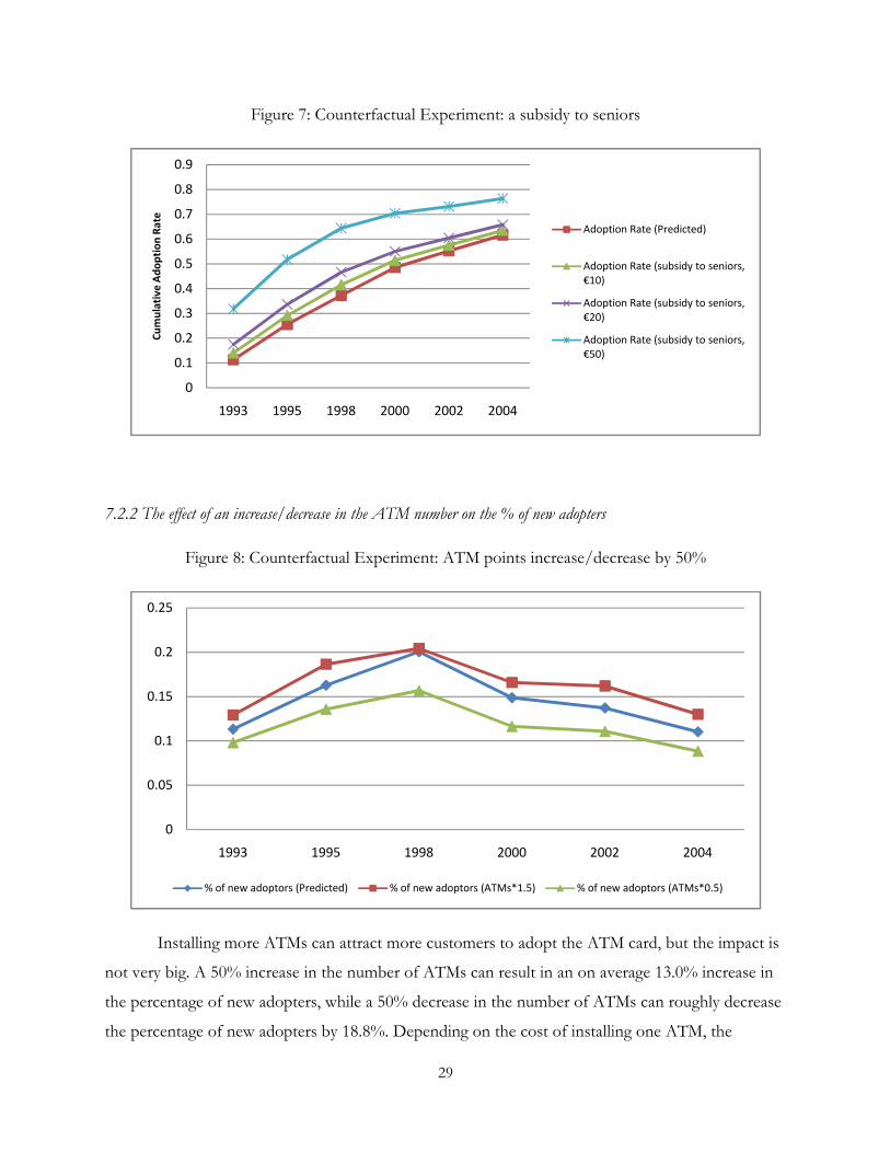
Figure 6: Counterfactual Experiment: a subsidy to seniors

Since it is mainly the elderly that have a low adoption rate, a subsidy targeting at the elderly

group (age > 50) is very effective: a €10 subsidy to the elderly can increase the average percentage of

new adopters to 18.9%; a €20 subsidy can raise the number to 24.2%; a €50 subsidy can make it

46.3%! Figures 7 and 8 show the impact of different amounts of subsidies to seniors on the

percentage of new adopters and the overall cumulative adoption rate, respectively.

0

0.1

0.2

0.3

0.4

0.5

0.6

1993 1995 1998 2000 2002 2004

% of new adoptors (Predicted) % of new adoptors (subsidy to seniors, €10)

% of new adoptors (subsidy to seniors, €20) % of new adoptors (subsidy to seniors, €50)

29

Figure 7: Counterfactual Experiment: a subsidy to seniors

7.2.2 The effect of an increase/decrease in the ATM number on the % of new adopters

Figure 8: Counterfactual Experiment: ATM points increase/decrease by 50%

Installing more ATMs can attract more customers to adopt the ATM card, but the impact is

not very big. A 50% increase in the number of ATMs can result in an on average 13.0% increase in

the percentage of new adopters, while a 50% decrease in the number of ATMs can roughly decrease

the percentage of new adopters by 18.8%. Depending on the cost of installing one ATM, the

0

0.1

0.2

0.3

0.4

0.5

0.6

0.7

0.8

0.9

1993 1995 1998 2000 2002 2004

Cu

mu

lati

ve

Ad

op

tio

n R

ate

Adoption Rate (Predicted)

Adoption Rate (subsidy to seniors,

€10)

Adoption Rate (subsidy to seniors,

€20)

Adoption Rate (subsidy to seniors,

€50)

0

0.05

0.1

0.15

0.2

0.25

1993 1995 1998 2000 2002 2004

% of new adoptors (Predicted) % of new adoptors (ATMs*1.5) % of new adoptors (ATMs*0.5)

30

subsequent maintenance cost, and competitors’ strategies, banks can decide how many new ATMs

to install in the future. It should be noted that we currently do not allow the number of ATMs to

lower the time costs of withdrawal. If this feature is incorporated, it is possible that the effect of this

experiment could be stronger. Another related experiment that we are investigating is to change the

growth rate of ATMs. This would allow us to examine the role of expectation.

7.2.3 The effect of an interest rate change on the % of new adopters

Figure 9: Counterfactual Experiment: interest rate increase/decrease by 20%

A higher interest rate would make it more costly to hold cash in hands, thus giving people

more incentives to adopt an ATM card; a lower interest rate would have the opposite effect. But the

magnitudes are not symmetric: as shown in Figure 9, a 20% interest rate increase would induce 6.9%

more non-adopters to adopt an ATM card, whereas a 20% interest rate cut would have made 10.8%

of new adopters decide not to adopt. Banks might want to learn the side effect of a promotional

interest rate increase: it can not only encourage people to deposit more, but it can also make non-

adopters more likely to consider getting an ATM card.

0

0.05

0.1

0.15

0.2

0.25

1993 1995 1998 2000 2002 2004

% of new adoptors (Predicted) % of new adoptors (interest*1.2) % of new adoptors (interest*0.8)

31

8 Concluding Remarks

This paper is motivated by a stylized fact of consumers’ adoption decisions - the elderly have

a much lower adoption rate of new technologies. Different reasons are offered in the literature and

these can be summarized as the elderly having a larger adoption cost. A larger adoption cost is one

explanation, and a shorter life horizon is another. Without a dynamic model taking people’s limited

life horizons into account, these two reasons cannot be separated out. This paper provides the first

attempt to disentangle these two reasons by allowing for age-specific adoption costs and

incorporating people’s different life horizons in a finite horizon dynamic model. The findings are

striking: the elderly do not have a larger adoption cost, so their lower adoption rate is probably

caused by their shorter remaining life horizons. With the help of a Baumol-Tobin type cash

inventory management model, we recover the initial adoption costs in 2002 euros and we find that a

static choice model underestimates the average adoption cost to a big extent.

Two limitations should be noted. First, we use a very simple calibration method to

transform adoption costs into monetary values, without considering time trend and individual

heterogeneity. Consequently, we can only interpret the estimated adoption costs as average costs.

Future research can make the calibration more flexible at the expense of a heavier computational

burden. Second, it might be worthwhile to more finely discretize the state space and allow for

normally distributed random coefficients by using, for example, the interpolation and simulation

method proposed by Keane and Wolpin (1994).

32

Appendix 1

The intuition for identification and why only a finite-horizon dynamic model can correctly estimate the initial adoption

cost

Suppose in the data we observe two individuals, Tom and Jerry. In 2000, both of them were 70 years

old. Tom adopted an ATM card in 2000, but Jerry did not. Suppose we can measure that Tom’s annual

adoption benefit was $10, while Jerry’s potential adoption benefit was $8. Let us further assume that the initial

adoption cost 0, was the same for both of them.

What kind of interval estimate of 0 can we get? In a static model, Tom and Jerry are assumed to be

myopic – they compare only their current benefit with the initial adoption cost. Because Tom adopted but

Jerry did not, we would infer that 0 is between $8 and $10. In an infinite horizon model with a 0.9 discount

rate, we would conclude that 0 is between $80 and $100, because we implicitly assume that people would live

forever by using an infinite horizon model. Realistically speaking, people would not be so myopic as to

consider only a one-period benefit, or be so naïve as to assume that they could live forever. They must realize

that they can enjoy the adoption benefit for many years, but not without an end. Suppose the terminal age is

80. After re-calculating their discounted future benefits, we could say that the initial adoption cost is between

$44 and $57.

This is a very simple model with only two individuals and no stochastic factors involved. But the

basic intuition has been clearly shown – we can back out the initial adoption cost if we can measure

individuals’ adoption benefits and if we know their adoption decisions. In addition, a static model tends to

underestimate the initial adoption cost and an infinite horizon dynamic model tends to overestimate the initial

adoption cost. Only a finite-horizon dynamic model can correctly estimate the initial adoption cost.

Appendix 2

Empirical evidence supporting the existence of learning cost in adopting ATM cards

In 2000 Survey, a special set of questions are asked:

If no-one in the household has a bank debit card or a credit card – or, if a card is not used at least three times a month

Why don’t you use debit cards or credit cards/why don’t you use them very much? (more than one answer is possible)

- service is complicated to use ........................................................ 1 (41.2%)

- fears of mistakes or fraud ............................................................. 2 (16.0%)

- used in the past and not satisfied .................................................. 3 (3.5%)

33

- too costly ...................................................................................... 4 (16.6%)

- the shopkeeper did not accept the card ......................................... 5 (0.5%)

- loss of discounts ........................................................................... 6 (0.92)

- don’t consider cards necessary...................................................... 7 (13.3%)

- prefer to use cash.......................................................................... 8 (5.8%)

- other (please specify): __________________________________ 9 (7.8%)

As one can see, at 42.2%, “service is complicated to use” is the primary reason why many Italians

don’t or seldom use ATM cards or credit cards. At 16.0%, “fears of mistakes or fraud” is another important

reason why people are afraid to use the new payment instruments. This evidence suggests that learning cost is

the major barrier preventing people from adopting these new instruments.

References

Adams, A.S. and K.A. Thieben, (1991): “Automatic Teller Machines and the Older Population.” Applied

Ergonomics, 22(2), 85-90.

Aguirregabiria, Victor and Pedro Mira (2007): "Dynamic Discrete Choice Structural Models: A Survey,"

Journal of Econometrics, forthcoming.

Attanasio, Orazio R., Guiso, Luigi, and Jappelli, Tullio (2002): “The demand for money, financial innovation, and the welfare cost of inflation: An analysis with household data,” Journal of Political Economy, 110(2), 317–351. Baumol, William J. (1952): "The Transactions Demand for Cash: an Inventory-Theoretic Approach," Quarterly Journal of Economics, 66, pp. 545-56. Canato, Anna and Nicoletta Corrocher (2004): “Information and communication technology: organisational challenges for Italian banks”, Accounting, Business and Financial History 14:3, 355–370. Dayton, C.M. and G.B. Macready (1988): “Concomitant-variable Latent-class Models”, Journal of the American Statistical Association, 83 (401), pp. 173–178. Eckstein, Z., and K. Wolpin (1989): "The Specification and Estimation of Dynamic Stochastic Discrete

Choice Models," Journal of Human Resources, 24, 562-598.

Ferrari, Stijn, Frank Verboven, and Hans Degryse (2007): “Investment and usage of new technologies:

evidence from a shared ATM network”, working paper, Catholic University of Leuven

Gilly, Mary C. and Valerie Zeithaml (1985): “The Elderly Consumer and Adoption of Technologies.” Journal

of Consumer Research, 12: 353-357.

Goettler, Ronald L. and Karen Clay (2007): “Tariff Choice with Consumer Learning: Sorting-Induced Biases

and Illusive Surplus”, working paper, CMU

Gordon, Brett (2007): “A Dynamic Model of Consumer Replacement Cycles in the PC Processor Industry”,

working paper, Columbia University

34

Gupta, S. and P.K. Chintagunta (1994): “On Using Demographic Variables to Determine Segment

Membership in Logit Mixture Models”, Journal of Marketing Research, 31, pp. 128–136.

Hall, Bronwyn H. and Beethika Khan (2003): “Adoption of New Technology” In Jones, Derek C., New Economy Handbook, Amsterdam: Elsevier Science, 2003. Hannan, Timothy H. and John M. McDowell (1984): “The Determinants of Technology Adoption: The Case of the Banking Firm” The RAND Journal of Economics, Vol. 15, No. 3., pp. 328-335. Hannan, Timothy H. and John M. McDowell (1987): “Rival Precedence and the Dynamics of Technology Adoption: An Empirical Analysis” Economica, New Series, Vol. 54, No. 214., pp. 155-171. Hatta, K. and Liyama, Y., (1991): “Ergonomic Study of Automatic Teller Machine Operability” International Journal of Human Computer Interaction 3(3), 295-309. Hester, Donald D., Calcagnini, Giorgio, and de Bonis, Ricardo (2001), “Competition through Innovation: ATMs in Italian Banks,” Rivista Italiana degli Economisti, (3), 359–381. Huynh, Kim P. (2007): “Financial Innovation and the Persistence of the Extensive Margin”, working paper, Indiana University Ishii, Joy (2005): “Compatibility, Competition, and Investment in Network Industries: ATM Networks in the Banking Industry”, working paper, Stanford University Keane, Michael P. and Kenneth I. Wolpin (1994): “The Solution and Estimation of Discrete Choice Dynamic Programming Models by Simulation and Interpolation: Monte Carlo Evidence,” The Review of Economics and Statistics, Vol. 74(4), pp. 648-672. Kerschner, P.A. & K. H. Chelsvig. (1984). “The Aged User and Technology,” in Dunkle, Ruth E., Haug Marie R., Rosenberg M. (eds) Communications Technology and the Elderly: Issues and Forecasts. New York: Springer Publishing Company, 135-144. Magnac, Thierry, and David Thesmar (2002): “Identifying Dynamic Discrete Decision Processes”, Econometrica, 70, 801-816. New York Times: “For Some Internet Users, It’s Better Late than Never”, March 25, 2004. OECD Indicators (2007): “Education at a Glance 2007” Orlandi, Eugenio (1989): “Computer Security Economics”, ICCST, Zurich, Switzerland, 107-111. Ricciarelli, Matteo (2007): “Transaction Privacy, Crime and Cash in the Purse: an Analysis with Household Data”, working paper. Rogers, W.A., Cabrera, E.F., Walker, N., Gilbert, D.K. and Fisk, A.D. (1996): “A Survey of Automatic Teller Machine Usage across the Adult Lifespan.” Human Factors 38, 156-166. Rust, John (1987): “Optimal Replacement of GMC Bus Engines: An Empirical Model of Harold Zurcher”, Econometrica, 55, 999-1033. Rust, John (1994): "Estimation of Dynamic Structural Models, Problems and Prospects: Discrete Decision

Processes", in C. Sims (ed.) Advances in Econometrics. Sixth World Congress, Cambridge University Press.

35

Rust, John and C. Phelan (1997): “How Social Security and Medicare Affect Retirement Behavior in a World of Incomplete Markets.” Econometrica, 65, 781-832.

Ryan, Stephen and Catherine Tucker (2007): “Heterogeneity and the Dynamics of Technology Adoption”, working paper, MIT

Saloner, Garth and Andrea Shepard (1995): “Adoption of Technologies with Network Effects: An Empirical Examination of the Adoption of Automated Teller Machines” The RAND Journal of Economics, Vol. 26, No. 3., pp. 479-501. Shcherbakov, Oleksandr (2007): “Measuring Consumer Switching Costs in the Television Industry”, working paper, University of Arizona

Sjuggerud, Steve (2005): “Interest Rate Forecast… The World’s Best Prediction for 2005 will Surprise You” The Investment U e-Letter, Issue # 401, Monday, January 10.

Song, Inseong, and Pradeep Chintagunta (2003): “A Micromodel of New Product Adoption with

Heterogeneous and Forward Looking Consumers: Application to the Digital Camera Category.” Quantitative

Marketing and Economics, 1, 371–407.

Swanson, Charles E., Kenneth J. Kopecky and Alan Tucker (1997): “Technology Adoption over the Life Cycle and Aggregate Technological Progress.” Southern Economic Journal, Vol. 63, No. 4, pp. 872-887. Tobin, James (1956): "The Interest Elasticity of Transactions Demand for Cash," The Review of Economics and Statistics, 38, August, pp. 241-247.

36

Table A1: AR(1) process for main state variables

State Variables -�,! ��,! (1,000 Lire) ��,! (1,000 Lire)

� − 1 0.9191

(0.0185)

0.9528

(0.00644)

0.9657

(0.00586)

Constant 0.1142

(0.00863) n.a. n.a.

� 0.1139 19.4462 11.6134

�� 0.8210 0.8794 0.9003

Range [0:0.1:1.5] [0:15:150] [0:10:100]

Number of grid points 16 11 11

Table A2: models with one segment

R=0.85, dynamic model R=0.9, dynamic model

parameter estimate s.d. estimate s.d.

.� (time trend) 2.6844** 0.4996 2.2861** 0.4101

?H@A (adoption benefit) 0.0902** 0.0103 0.0794** 0.009

?B (# of ATMs) 0.9018** 0.324 0.7935* 0.3204

0�,� (adoption cost in segment 1) 13.0829** 1.5635 16.3025** 1.8322

g� (age-specific adoption cost, age>50) -0.0217 0.0182 -0.1036** 0.0257

g� (age-specific adoption cost, age<50) -0.0227* 0.0115 -0.033* 0.013

-ll 829.489

839.948

N 1961

1961

AIC 1670.978

1691.896

BIC 1678.733

1699.651

37

Table A3: models with three segments

R=0.85, dynamic model R=0.9, dynamic model

parameter estimate s.d. estimate s.d.

.� (time trend) 3.1638** 0.8882 2.5156** 0.6651

?H@A (adoption benefit) 0.1156** 0.0193 0.0977** 0.0136

?B (# of ATMs) 1.8292** 0.6494 2.0032** 0.6764

0�,� (adoption cost in segment 1) 11.8927** 2.2483 14.303** 2.9898

Log(0�,� − 0�,�)

(log(adoption cost difference between segments 2 and 1)) -0.6188 3.2667 1.8029** 0.5583

Log(0�,� − 0�,�)

(log(adoption cost difference between segments 3 and 2)) 1.6386** 0.173 0.0725 7.743

g� (age-specific adoption cost, age>50) 0.0016 0.0289 -0.0635 0.0426

g� (age-specific adoption cost, age<50) -0.0133 0.0163 -0.0233* 0.0095

m�� -0.531 0.5411 0.8386 3.8343

m8|}� 0.1734 0.5409 -0.1535 0.3659

mB~f!�� -2.5596* 1.2623 2.2363 24.5916

m|���,� (none) -2.1159** 0.3795 -2.8384 2.8238

m|���,� (elementary) -2.5364 1.6958 -1.9436 3.7252

m|���,� (middle school) -1.0292 0.8105 -1.1051 3.8374

m�� -2.4221* 1.2248 0.9751 8.7846

m8|}� 0.0383 0.3259 -0.6911 0.7078

mB~f!�� 0.3974 0.522 4.7594 24.8495

m|���,� (none) -1.0373 0.6794 -3.4609 10.3246

m|���,� (elementary) 0.9774 0.8415 -3.154 10.9491

m|���,� (middle school) 1.3812+ 0.8191 -2.4499 8.8966

-ll 811.437

812.383

N 1961

1961

AIC 1662.874

1664.766

BIC 1688.724

1690.616

38

Figure A1: Number of ATMs in Italy, 1991-1999

Source: Hester et al (2001)

Figure A2: Ratio of ATMs to Branches, 1991-1999

Source: Hester et al (2001)

Figure A3: Cumulative Adoption Rate of ATM Card, 1991-2004

Source: SHIW 1991-2004

0

2000

4000

6000

8000

10000

12000

1991 1992 1993 1994 1995 1996 1997 1998 1999

Northwest

Northeast

Central

South

Islands

0

0.2

0.4

0.6

0.8

1

1.2

1.4

1991 1992 1993 1994 1995 1996 1997 1998 1999

Northwest

Northeast

Central

South

Islands

Total

0.3190.357

0.400

0.4850.521

0.554 0.578

1991 1993 1995 1998 2000 2002 2004

39

Figure Series A4

Age histograms for the panel (1991-2004)

Age Histogram: 1991 Age Histogram: 1993 Age Histogram: 1995

Age Histogram: 1998 Age Histogram: 2000 Age Histogram: 2002

Age Histogram: 2004

0.01

.02

.03

Density

20 40 60 80 1001991

0.005

.01

.015

.02

.025

Density

20 40 60 80 1001993

0.01

.02

.03

Density

20 40 60 80 1001995

0.01

.02

.03

Density

20 40 60 80 1001998

0.005

.01

.015

.02

.025

Density

20 40 60 80 1002000

0.005

.01

.015

.02

.025

Density

20 40 60 80 1002002

0.01

.02

.03

Density

20 40 60 80 1002004

40

Figure Series A5

% of new adopters over non-adopters in the previous period by age and education (1993-2004)

0

0.05

0.1

0.15

0.2

0.25

0.3

0.35

up to 50 years from 51 to 65 years more than 65 years

1993

none elementary school middle school high school

0

0.1

0.2

0.3

0.4

up to 50 years from 51 to 65 years more than 65 years

1995

none elementary school middle school high school

0

0.1

0.2

0.3

0.4

0.5

0.6

up to 50 years from 51 to 65 years more than 65 years

1998

none elementary school middle school high school

41

0

0.1

0.2

0.3

0.4

up to 50 years from 51 to 65 years more than 65 years

2000

none elementary school middle school high school

0

0.1

0.2

0.3

0.4

0.5

0.6

up to 50 years from 51 to 65 years more than 65 years

2002

none elementary school middle school high school

0

0.05

0.1

0.15

0.2

0.25

0.3

0.35

up to 50 years from 51 to 65 years more than 65 years

2004

none elementary school middle school high school

42

Figure A6: Gender-specific survival probabilities

0

0.2

0.4

0.6

0.8

1

1.2

20 23 26 29 32 35 38 41 44 47 50 53 56 59 62 65 68 71 74 77 80 83 86 89 92 95 98

male female