dynamics of chemical degradation in water using ...dynamics of chemical degradation in water using...

Air Force Institute of TechnologyAFIT Scholar

Theses and Dissertations

9-14-2017

Dynamics of Chemical Degradation in WaterUsing Photocatalytic Reactions in an UltravioletLight Emitting Diode ReactorJohn E. Stubbs

Follow this and additional works at: https://scholar.afit.edu/etd

Part of the Environmental Engineering Commons

This Dissertation is brought to you for free and open access by AFIT Scholar. It has been accepted for inclusion in Theses and Dissertations by anauthorized administrator of AFIT Scholar. For more information, please contact [email protected].

Recommended CitationStubbs, John E., "Dynamics of Chemical Degradation in Water Using Photocatalytic Reactions in an Ultraviolet Light Emitting DiodeReactor" (2017). Theses and Dissertations. 779.https://scholar.afit.edu/etd/779

https://scholar.afit.edu?utm_source=scholar.afit.edu%2Fetd%2F779&utm_medium=PDF&utm_campaign=PDFCoverPages

https://scholar.afit.edu/etd?utm_source=scholar.afit.edu%2Fetd%2F779&utm_medium=PDF&utm_campaign=PDFCoverPages

https://scholar.afit.edu/etd?utm_source=scholar.afit.edu%2Fetd%2F779&utm_medium=PDF&utm_campaign=PDFCoverPages

http://network.bepress.com/hgg/discipline/254?utm_source=scholar.afit.edu%2Fetd%2F779&utm_medium=PDF&utm_campaign=PDFCoverPages

https://scholar.afit.edu/etd/779?utm_source=scholar.afit.edu%2Fetd%2F779&utm_medium=PDF&utm_campaign=PDFCoverPages

mailto:[email protected]

DYNAMICS OF CHEMICAL DEGRADATION IN WATER USING PHOTOCATALYTIC REACTIONS IN AN ULTRAVIOLET LIGHT EMITTING

DIODE REACTOR

DISSERTATION

John E. Stubbs, Lieutenant Colonel, USAF AFIT-ENV-DS-17-S-052

DEPARTMENT OF THE AIR FORCE

AIR UNIVERSITY

AIR FORCE INSTITUTE OF TECHNOLOGY

Wright-Patterson Air Force Base, Ohio

DISTRIBUTION STATEMENT A. APPROVED FOR PUBLIC RELEASE; DISTRIBUTION UNLIMITED.

The views expressed in this thesis are those of the author and do not reflect the official policy or position of the United States Air Force, Department of Defense, or the United States Government. This material is declared a work of the U.S. Government and is not subject to copyright protection in the United States.

AFIT-ENV-DS-17-S-052

DYNAMICS OF CHEMICAL DEGRADATION IN WATER USING PHOTOCATALYTIC REACTIONS IN AN ULTRAVIOLET LIGHT EMITTING

DIODE REACTOR

DISSERTATION

Presented to the Faculty

Graduate School of Engineering and Management

Air Force Institute of Technology

Air University

Air Education and Training Command

in Partial Fulfillment of the Requirements for the

Degree of Doctor of Philosophy

John E. Stubbs, BS, MS

Lieutenant Colonel, USAF

September 2017

DISTRIBUTION STATEMENT A. APPROVED FOR PUBLIC RELEASE; DISTRIBUTION UNLIMITED.


DYNAMICS OF CHEMICAL DEGRADATION IN WATER USING PHOTOCATALYTIC REACTIONS IN AN ULTRAVIOLET LIGHT EMITTING DIODE REACTOR

John E. Stubbs, BS, MS

Lieutenant Colonel, USAF

Committee Membership:

Willie F. Harper, Jr., PhD

Chairman

LTC Douglas R. Lewis, USA, PhD Member

Matthew L. Magnuson, PhD

Member

Michael E. Miller, PhD

Member

ADEDJI B. BADIRU, PhD

Dean, Graduate School of Engineering and Management

iv


Abstract

Water scarcity and contamination are challenges to which the United States

homeland is not shielded and policies and technologies that support a “Net Zero” water

use posture will become increasingly critical. This work examined ultraviolet (UV) light

emitting diodes (LED) and hydrogen peroxide in an advanced oxidation process in

support of a USAF net zero water initiative. A UV LED reactor was used for degradation

of soluble organic chemicals. Linear relationships were observed between input drive

current, optical output power, and apparent first order degradation rate constants. When

drive current was varied, apparent first order degradation rates depended on chemical

identities and the drive current. When molar peroxide ratios were varied, kinetic profiles

revealed peroxide-limited or radical-scavenged phenomena. Accounting for molar

absorptivity helped explain chemical removal profiles. Observed degradation kinetics

were used to compare fit with molecular descriptors from published quantitative structure

property relationship (QSPR) models. A new QSPR model was built using zero point

energy and molar absorptivity as novel predictors. Finally, a systems architecture was

used to describe a USAF installation net zero water program and proposed areas where

UV LED reactors might be integrated. Facility-level wastewater treatment was found to

be the most feasible near-term application. This research is the first UV LED-based AOP

study to identify linear power-kinetics relationships, determine optimum molar peroxide

ratios, and reveal the complexity of molar absorptivity in shaping treatment profiles.

v


To God, my family, and the betterment of future generations.

vi

Acknowledgments

I am forever grateful to my research advisor, Dr. Willie Harper, for his wisdom,

patience, and guidance. To my research committee members, Dr. Michael Miller, Dr.

Douglas Lewis, and Dr. Matthew Magnuson, thank you for your critical review and

willingness to give your time and expertise to the process. Thanks also to Dr. Daniel

Felker for countless hours of laboratory support and analytical method development, Lt

Col David Kempisty for lending an ear when needed, Ms. Kandace Bailey for helping

with subtle secrets of the lab, and Mr. Morgan Russell for sharing lab space, equipment,

and time.

Most importantly, thanks to God and my family. This would not have been

possible without a solid spiritual grounding and the support of my wife and children.

John E. Stubbs

vii

Table of Contents

Page

Abstract .............................................................................................................................. iv

Acknowledgments.............................................................................................................. vi

List of Figures .................................................................................................................... ix

List of Tables .................................................................................................................... xii

I. Introduction .....................................................................................................................1

1.1. Motivation .............................................................................................................1

1.2. Problem..................................................................................................................3

1.3. Research Objectives and Scope .............................................................................4

1.4. Contributions .........................................................................................................6

1.5. Document Outline .................................................................................................8

II. The Effect of Operating Parameters on Kinetics in an UV LED/H2O2 Advanced

Oxidation Process ................................................................................................................9

2.1. Introduction .........................................................................................................10

2.2. Materials and Methods ........................................................................................19

2.3. Results and Discussion ........................................................................................34

2.4. Conclusions .........................................................................................................58

III. Quantitative Structure Property Relationship Models for Predicting Degradation

Kinetics for a Ultraviolet Light Emitting Diode/Peroxide Advanced Oxidation Process .60

3.1. Introduction .........................................................................................................61

3.2. Materials and Methods ........................................................................................68

3.3. Results and Discussion ........................................................................................72

3.4. Conclusions .......................................................................................................100

IV. UV LED AOP Application in a USAF Net Zero Water Program – A Systems

Architecture View ............................................................................................................101

viii

4.1. Introduction .......................................................................................................102

4.2. Background........................................................................................................103

4.3. Net Zero Water System Model ..........................................................................109

4.4. Discussion..........................................................................................................118

4.5. Conclusions .......................................................................................................127

V. Conclusions ................................................................................................................129

5.1 Discussion..........................................................................................................129

5.2 Future Work.......................................................................................................132

VI. Appendix A ...............................................................................................................135

VII. Appendix B..............................................................................................................184

Bibliography ....................................................................................................................214

Vita ..................................................................................................................................223

ix

List of Figures

Figure Page

Figure 1. Complete UV LED reactor assembly showing pairing of central cylinder and

spherical end caps with heat sinks. ............................................................................ 23

Figure 2. View of an end cap removed from the reactor showing LED placement. ........ 24

Figure 3. Schematic depicting complete experimental setup. .......................................... 27

Figure 4. View of reactor endcap removed showing stir bar in middle of tube and LED at

distal end. ................................................................................................................... 28

Figure 5. Comparison of optical output power achieved from input drive current. ......... 36

Figure 6. Linear relationship between apparent degradation rate constant and drive

current. Three example linear fits are shown. ........................................................... 38

Figure 7. The effect of drive current on Erythrosine B removal. ..................................... 44

Figure 8. The effect of drive current on the degradation of dyes. .................................... 46

Figure 9. The effect of molar peroxide ratio on Brilliant Blue FCF removal at 200 mA. 51

Figure 10. The effect of molar peroxide ratio on Erythrosine B removal at 80 mA. ....... 52

Figure 11. The effect of molar peroxide ratio on TBA removal at 120 mA. .................... 53

Figure 12. Relationship between CSTR model fit and molar absorptivity. ..................... 57

Figure 13. Actual versus predicted degradation rate constants utilizing Wang et al.

descriptors with the full data set. ................................................................................ 74


descriptors with the dye data set. ............................................................................... 75


descriptors with the achromatic chemical data set. .................................................... 76

x

Figure 16. Actual versus predicted degradation rate constants utilizing Jin et al.


Figure 17. Actual versus predicted degradation rate constants utilizing Tang descriptors

with the full data set. .................................................................................................. 81


with the dye data set. .................................................................................................. 82


with the achromatic chemical data set. ...................................................................... 83

Figure 20. Actual versus predicted degradation rate constants utilizing Kusic et al.



descriptors and omitting malathion and Allura Red AC. ........................................... 87


descriptors with the dye data set. ............................................................................... 88

Figure 23. Actual versus predicted degradation rate constants utilizing Sudhakaran and

Amy, 2012 descriptors with the full data set. ............................................................. 90


Amy, 2013 descriptors with the full data set. ............................................................. 92


Amy, 2013 descriptors with the dye data set. ............................................................ 93


Amy, 2013 descriptors with the achromatic chemical data set. ................................. 94

xi

Figure 27. Actual versus predicted degradation rate constants utilizing Zero Point Energy

as a descriptor with the full data set. .......................................................................... 98

Figure 28. Actual versus predicted degradation rate constants utilizing Zero Point Energy

and molar absorptivity as descriptors with the full data set. ...................................... 99

Figure 29. Capability taxonomy for a USAF installation net zero water program. ........ 110

Figure 30. Hybrid systems view of a net zero water program at a USAF installation with

boundaries at the installation and facility level. ....................................................... 113

Figure 31. Operational activity lanes for four areas of potential UV LED/H2O2 advanced

oxidation treatment within a net zero water program. ............................................. 115

Figure 32. Mass balance relationships between facility influent, recycle, and effluent

flows; Q2/Q1 represents a recycle ratio in water reuse scenarios. ........................... 123

Figure 33. The effect of facility size and recycle ratio on the required first order rate

constant. ................................................................................................................... 124

xii

List of Tables

Table Page

Table 1. Basic information and properties pertaining to dyes and achromatic chemicals

used in experiments. ................................................................................................... 21

Table 2. Output characteristics of UV LEDs utilized in reactor experiments. ................. 35

Table 3. Calculated photon production rate for each drive current level. ......................... 40

Table 4. Molecular descriptors utilized in QSPRs built from traditional mercury lamp

AOP data. ................................................................................................................... 71

Table 5. Parameters and tests of statistical significance for new models built with zero

point energy and molar absorptivity. ......................................................................... 97

1

DYNAMICS OF CHEMICAL DEGRADATION IN WATER USING

PHOTOCATALYTIC REACTIONS IN AN ULTRAVIOLET LIGHT EMITTING

DIODE REACTOR

I. Introduction

1.1. Motivation

The United States Air Force (USAF) Energy Strategic Plan identifies water as a

critical asset and incorporates water into a strategy seeking to balance resource

consumption, production, and conservation (US Air Force 2013). It sets a foundation for

all Airmen to make energy and water conservation a part of operational considerations.

The USAF generally consumes around 27 billion gallons of water per year at an annual

cost of $150 million, and energy utilized in water treatment and delivery contributes to an

overall $9 billion annual energy cost. The plan establishes energy priorities of improved

resilience, reduced demand, assured supply, and fosters an energy aware culture. This

culture should lead the way toward a future state where the USAF identifies and

integrates energy and water efficiency throughout business and planning processes,

promotes integration of new technologies to reduce costs and increase effectiveness, and

leverages investments in a constrained resource environment. In the near term, the USAF

has established a “Net Zero Initiative” where an installation consumes no more energy

than is generated on the installation, and potable water demand is reduced by capturing

and reusing, repurposing, or recharging an amount of water that is greater than or equal to

the volume of water the installation uses. The initiative is designed to achieve a federal

2

zero net energy goal by 2030 for new facility construction and alterations (US Air Force

2013).

Furthermore, the US military has been engaged globally since World War I with

forces deployed worldwide supporting a spectrum of operations from humanitarian crises

to wartime contingencies. The reach of the military has continued to grow in recent

decades with a need for simultaneous peacetime and wartime operations, and it is

inevitable that the need for global engagement will continue in coming decades. An

adequate supply of clean, safe drinking water is critical to the success of US forces

carrying out missions in support of these operations. Water is necessary for hydration,

food preparation, medical treatment, hygiene, construction, decontamination,

maintenance, and many additional tasks. Water supply functions enable freedom of

action, extend operational reach, and prolong operational endurance (US Army 2015).

Water supply to both large, established bases and forward-deployed personnel is one of

the largest logistics requirements of the military; however, water is also a limited

resource that can cause disruptions and instability in numerous regions across the world.

Conserving energy and water not only results in savings to the USAF, it can also mitigate

increased competition in water-scarce regions that provoke potential conflicts (US Air

Force 2013):

“Optimizing energy and water use not only saves resources and money, but is

also a force multiplier that allows the Air Force to apply resources and airpower

more efficiently and effectively.”

3

1.2. Problem

In an operational context that seeks to balance fiscal constraint with sustained

global operations, the USAF needs to consider emerging technologies for water treatment

that provide necessary water supply while simultaneously reducing energy costs and

striving for net zero consumption. Once such technological advancement is recent

development of energy efficient ultraviolet (UV) light emitting diodes (LED) as a

replacement for high energy consuming mercury vapor lamps in advanced oxidation

processes (AOP) utilizing hydrogen peroxide (H2O2). UV LED based water treatment is

now possible. However, little data is available on the use of UV LED/H2O2 for the

destruction of soluble organics (Duckworth, et al. 2015; Scott, et al. 2016). There is a

need to expand understanding of organic chemical destruction work to a greater number

of chemicals to improve the fundamental understanding of this process. This study seeks

to expand upon UV LED AOP treatment for the degradation of soluble organic

compounds.

There is also a general need to assess tools that can be used to predict chemical

degradation in UV AOPs in general, and particularly UV LED-based processes.

Quantitative structure-property relationships (QSPR) can provide such a tool. The

advantage of the QSPR approach, once an acceptable model is developed, is the ability to

predict removal relative to baseline conditions strictly on the basis of the compound

structure without further laboratory testing. Several previous studies have developed

QSPRs relating chemical structure to degradability (Sudhakaran, et al. 2012; Chen, et al.

2007; Kusic, et al. 2009; Lee and von Gunten 2012; Meylan and Howard 2003;

4

Minakata, et al. 2009; Ohura, et al. 2008; Sudhakaran and Amy 2013; Wang, et al. 2009).

QSPRs have not been evaluated for UV LED-based reactors.

1.3. Research Objectives and Scope

1.3.1. Objectives

1.3.1.1. The first objective is to determine the effect of key reactor operating

parameters on the reaction mechanisms associated with the advanced oxidation of soluble

organic compounds with UV LEDs. The supporting tasks are:

• Determine the effect of peroxide stoichiometry on typical soluble organic

chemical degradation profiles

• Determine the effect of LED output power on soluble organic chemical

degradation profiles

• Evaluate optimality of degradation rate/input power/H2O2 combinations

Hypothesis #1 is that reactions with chemicals involving chain-terminating steps (i.e.,

those that stop the propagation of hydroxyl radicals) are expected to slow down at a faster

rate as the availability of light and H2O2 is decreased, as compared to chemicals not

involving chain-terminating steps. These chain-terminating steps cause peroxide to

become consumed, which in turn prevents the regeneration of hydroxyl radicals.

Chemicals that involve chain-terminating steps include tert-butyl alcohol.

1.3.1.2. The second objective is to evaluate QSPRs for the advanced oxidation of

soluble organic compounds with UV LEDs. The supporting tasks are:

• Determine apparent first order degradation rate constants for test chemicals

5

• Determine molecular descriptors for test chemicals

• Assess apparent first order degradation rate constant fit to molecular descriptors

used in existing QSPRs in the literature

• Utilize multivariate methods to develop and test new basic QSPRs

Hypothesis #2 is that the observed reaction rate can be best predicted using frontier

electron density (FED). The rationale for this is as follows. FED is a part of electronic

theory, where the reactivity of a chemical can be explained by the distribution of

electrons in a molecule (Fukui 1981). FED theory involves determining the highest

occupied molecular orbital (HOMO) and the lowest unoccupied molecular orbital

(LUMO) interaction. For electrophilic reactions, HOMO densities govern reaction

pathways, while for nucleophilic reactions, the LUMO densities govern reaction

pathways. Additionally, Koopman’s theorem states that ionization energy (or ionization

potential) of a molecule is equal to the negative of the HOMO energy. Following this

hypothesis, the observed reaction rates should be greatest where the HOMO-based FED

is highest (or conversely, the ionization energy is lowest).

1.3.1.3. The third objective is to use systems engineering principles to propose

appropriate applications of UV LED-based reactors in support of specific water quality

applications. The supporting tasks include:

• Identify the scope of near term water quality challenges in USAF

• Identify opportunities to couple AOP with other existing and emerging

technologies (e.g. microbial fuel cells)

6

• Build a conceptual systems architecture view illustrating areas of potential UV

LED/H2O2 technology integration within a “Net Zero” water program

Hypothesis #3 is that the most promising near term UV LED applications will involve

those that leverage existing technologies to treat low flow waste streams to remove

chemicals that do not include chain terminating steps.

1.3.2. Scope

The scope of this research is limited to degradation of six dyes and five

achromatic chemicals by UV LED/H2O2 AOP. In this work, achromatic is used

explicitly to denote the chemicals are without color (e.g. they do not have a visible

spectrum). The scope is also constrained to the specific reactor and associated reactor

parameters utilized in the experiments; however, the results of this study may be more

broadly applicable to optimizing reactor design and operating parameters. Degradation

rate constants derived from an experiment are limited in scope to the conditions under

which the experiment was conducted (e.g. flow, volume, chemical concentrations, UV

intensity, etc.). Additionally, QSPR development is limited to the domain of applicability

of the test compounds used to develop the model. Development of a systems architecture

view is hypothetical in nature and must be customized to specific installation

requirements.

1.4. Contributions

This research effort expands significantly upon prior UV LED AOP studies. The

initial emphasis was on creating a reactor platform that allowed for comparative

7

UV/H2O2 AOP degradation analysis of multiple dyes and achromatic chemicals across

varying H2O2 concentrations and light intensities. Reactor operating parameters were

adjusted to assess models of optimal efficiency and gain insight into hydroxyl radical

production and associated degradation rates. Molecular descriptors of the dyes and

achromatic chemicals used were assessed for their predictive capability and molecular

descriptors used in existing QSPRs were assessed for their fit to the UV LED domain.

Several specific contributions to the existing body of knowledge come from this

research:

1. A comparison of degradation kinetics for six dyes and five achromatic

chemicals reacted in the same well-mixed, flow through reactor platform under the same

reaction conditions.

2. An understanding of any relationships between degradation kinetics and

molecular descriptors for six dyes and five achromatic chemicals and development of a

novel QSPR.

3. An assessment of the adequacy of existing QSPR models relating molecular

descriptors to apparent first order degradation rate constants.

4. An understanding of the impact of molar absorptivity of a dye at peak LED

output wavelength on overall reaction kinetics.

5. A comparative analysis of the efficiency tradeoffs between optical output

power, H2O2 concentration, and apparent first order degradation rate constants.

8

1.5. Document Outline

This dissertation contains five chapters. Chapter I provided the motivation,

problem statement, research questions, scope, and tasks. Chapters II-IV are presented in

scholarly format where each chapter can stand alone and be made ready for publication in

journals/conference proceedings, although currently their level of detail is designed for

this dissertation. Chapter II addresses research objective 1 and presents the results of

reactor operating parameter effects on degradation kinetics and analyzes comparative

kinetics of the various test compounds. Chapter III addresses research objective 2 in

assessing suitability of molecular descriptors used in existing QSPR models and their fit

to the UV LED domain. Chapter III also discusses efforts to build new basic QSPRs

from the apparent first order degradation rate constants and molecular descriptors

relevant to the test compounds. Chapter IV reviews near term water challenges for the

USAF and introduces a proposed “Net Zero” systems architecture view, integrating UV

LED AOP with other treatment technologies. Finally, Chapter V offers concluding

discussion and suggestions for future work.

9

II. The Effect of Operating Parameters on Kinetics in an UV LED/H2O2 Advanced Oxidation Process

Keywords

Ultraviolet (UV), light emitting diode (LED), advanced oxidation process (AOP), hydrogen peroxide (H2O2)

Abstract

A bench-scale reactor utilizing UV LEDs as an energy source in a UV/H2O2 advanced oxidation process was used for the degradation of 6 dye and 5 achromatic organic compounds. As individual LEDs provide significantly less total output power as compared to mercury lamps, it is important to understand parameters that impact the production and efficient utilization of the available photons. There was a linear relationship between the input drive current, optical output power, and the apparent first order degradation rate constant, consistent with first principles from quantum mechanics. When the drive current was systematically varied, the apparent first order degradation rate constants depended on the identity of the test compound and the drive current, and were between 0.003 min-1 - 1.078 min-1. There was also a linear relationship between the drive current and the degradation extent. When the molar peroxide ratio was systematically varied, the kinetic profiles revealed either peroxide-limited or radical-scavenged phenomena, consistent with existing literature. The optimum molar peroxide ratios were at or near 500 mole H2O2/mole test compound for most of the dyes, but for erythrosine B (EB), the best molar peroxide ratios tested were in the range of 2500-3000 mole H2O2/mole EB, likely because of its relatively high molar absorptivity ratio. Accounting for molar absorptivity also helped to explain the shape of the removal profiles associated with EB and tartrazine, as well as the regression coefficients associated with the model fitting of experimental data. In contrast, the optimal molar peroxide ratios were at or near 100 mole H2O2/mole test compound for achromatic chemicals with the lowest molar absorptivity. This research is the first UV LED-based AOP study to identify linear power-kinetics relationships, determine optimum molar peroxide ratios, and reveal the complex role of molar absorptivity in shaping the speed and extent of treatment.

10

2.1. Introduction

Advanced oxidation processes are important to the water treatment community,

because they can degrade a wide range of toxic chemical compounds (Crittenden et al.

2012). This study is focused on the UV/H2O2-based AOP and seeks to implement

UV/H2O2 AOPs with light emitting diodes (LEDs) as an alternative to conventional

mercury lamps. Hydroxyl radicals are produced when hydrogen peroxide absorbs UV

light at a wavelength < 280 nm, resulting in the rapid and non-selective degradation of

many soluble organic compounds and their byproducts (Minakata, et al. 2009)

(Andreozzi, et al. 1999). UV light must be available at an energy level high enough to

achieve oxygen-to-oxygen bond cleavage in the peroxide molecule, resulting in the

production of two hydroxyl radicals (Benjamin and Lawler 2013; Luo 2007). Reactions

with hydroxyl radicals are among the fastest aqueous phase reactions known (Dorfman

and Adams 1973).

UV LEDs exhibit several advantages over mercury lamps including small size,

light weight, physical durability, and lack of hazardous components (Ibrahim, et al.

2014). UV LEDs may also have a comparative disadvantage currently as the output

power of an individual LED is significantly lower than traditional lamps; however,

manufacturing improvements are continually increasing the comparative output power of

LED sources (Gallucci 2016). Presently available UV LED models provide optical

output power in the milliwatt (mW) range, whereas low pressure mercury lamps have

output of 30-600 watts (W) and medium pressure lamps between 1-12 kilowatts (kW)

(Atlantium Technologies 2017). However, given their compact size and point source

configuration, UV LEDs can be placed more flexibly and can be arranged in multi-LED

11

arrays to achieve increased overall output power. UV LEDs may have another

comparative advantage in the ability to select LEDs with specific desired output

wavelengths, whereas low pressure lamps are limited to a single 254 nm wavelength and

medium pressure lamps emit a broad spectrum covering 200-320 nm.

The success of the UV LED/H2O2 AOP depends on the structure of the chemical

compound, the amount of peroxide in solution, and the LED output power. These factors

can be systematically tested in an attempt to understand the more general trends that

impact chemical degradation. The objective of this study is to evaluate the effect of

reaction stoichiometry, molecular structure, and optical output power on the UV

LED/H2O2 process.

2.1.1. General Characteristics of the UV/H2O2 Advanced Oxidation Process

UV-peroxide advanced oxidation processes produce hydroxyl radicals through a

photocatalytic reaction initiated when H2O2 absorbs UV light at a wavelength (λ) < 280

nm. Critical to the initiation of this process is ensuring adequate exposure to UV light at

an energy high enough to achieve cleavage of the O-O bond in the H2O2 molecule. This

cleavage leads to the formation of two hydroxyl radicals (Benjamin and Lawler 2013). A

representative published value for the energy required to activate O-O bond dissociation

is 210.66 ± 0.42 kJ/mol (Luo 2007). Energy per unit time provided by the UV LEDs and

residence time of solution within the light distribution will together determine whether

there is sufficient energy for cleavage to occur. Compared to medium pressure and low

pressure mercury UV lamps, individual LEDs produce significantly less optical output

power making this a critical comparison and design factor.

12

The equations governing the generation, interaction, and termination of hydroxyl

radicals are well-researched and documented in the literature (Chang, et al. 2010;

Crittenden, et al. 1999; Edalatmanesh, et al. 2008; Ghafoorim, et al. 2014; Grcic, et al.

2014; Mariani, et al. 2013; Wols and Hofman-Caris 2012). When the H2O2 molecule

absorbs sufficient UV energy at the proper wavelength, the initiated reaction produces

two hydroxyl radicals as shown below:

OHhvOH •→+ 222 The hydroxyl radicals further propagate through the following reactions:

OHHOOHOH 2222 +→+ ••

22222 OOHOHHOOH ++→+ •• −•+• +→ 22 OHHO

Radical products are then terminated through the following reactions:

222 OHOH →•

22222 OOHHO +→•

222 OOHHOOH +→+ ••

22 OOHOOH +→+ −−••

During this process, the hydroxyl radicals will rapidly and non-selectively react

with organic compounds they encounter. Subsequent radical production in the chain can

continue to attack the organic material until it is mineralized. As an example in the

context of this research, the hydroxyl radicals will react with a dye and mineralize it as

seen below:

productsdyeOH →+•

13

Hydroxyl radicals can also react with each other. These fast reactions result in short

lifetimes of the hydroxyl radicals (Gligorovski, et al. 2015; Benjamin and Lawler 2013).

Therefore, mixing and proper UV fluence is critical to the effectiveness of hydroxyl

radicals as oxidants (USEPA 1999).

Hydroxyl radicals can react with the organic compounds by one of three

mechanisms: 1) hydrogen abstraction (H removal), 2) hydroxylation (OH addition), or 3)

oxidation without transfer of atoms (Buxton, et al. 1988). In general, hydrogen

abstraction is likely to occur in saturated molecules (those with no double bonds) and

hydroxylation is likely to occur in unsaturated molecules (those with double bonds);

however, this is not always the case and oxidation without atom transfer can occur

(Benjamin and Lawler 2013).

2.1.2. Effect of Reactant Concentrations and Solution pH

Prior studies suggest that starting molar ratios of H2O2 to dye must be considered

to avoid creating a condition that is limited by one of the reactants. In a study that

degraded Basic Violet 16 dye with UV/H2O2, varying the starting dye concentration

while holding H2O2 constant had a pronounced impact on reducing degradation rate as

dye concentration increased beyond a critical point. Additionally, increasing

concentration of H2O2 improved degradation to a critical point, thereafter additional H2O2

decreased the reaction rate due to H2O2 self-scavenging of hydroxyl radicals (Rahmani, et

al. 2012). The first point is supported in other studies related to UV/H2O2 degradation of

dyes (Chang, et al. 2010; Narayansamy and Murugesan 2014). The second point is also

supported elsewhere in literature, indicating that too low a level of H2O2 appears to limit

14

generation of hydroxyl radicals, while too much H2O2 appears to scavenge hydroxyl

radicals (Sharma 2015; Muruganandham and Swaminathan 2004; Oancea and Meltzer

2013).

An additional flaw in selecting incorrect starting quantities of reactants is the

potential to violate assumptions underlying a pseudo-first order kinetic reaction model.

In a pseudo-first order model, a fundamental requirement is that one of the reactants is

available in abundance over the other reactant so that it may be essentially treated as a

constant. Violating this assumption with stoichiometric adjustments may create a bias in

the model (Hartog, et al. 2015).

A point regarding stoichiometry can also be made with the relationship between

H2O2, the quantity of hydroxyl radicals produced, and the quantity of hydroxyl radicals

actually available for reaction. General chemistry principles indicate the generation of

two moles of hydroxyl radicals from each mole of hydrogen peroxide. However, it has

been found that in aqueous solutions, a solvent “cage effect” can trap up to 50% of the

hydroxyl radicals, reducing the number available for oxidation (Oppenlander 2003).

Another consideration in the AOP process is the effect that the solution’s pH may

have on the efficiency of hydroxyl radical production. H2O2 has a pKa of 11.8 and

dissociation will increase as the solution becomes more basic as shown below:

−+ +↔ 222 HOHOH

There is literature to suggest that changing pH can affect the efficacy of hydroxyl

radical degradation of dyes when other parameters are held constant. In one such study,

the azo dye Reactive Orange 4 was degraded using H2O2/UV. The effect of varying pH

15

over a range of 2-8 and changing the amount of H2O2 between 5-25 mmol were studied.

Maximum degradation was achieved at pH = 3 with sharp decline as pH was adjusted

higher. Degradation increased along with increasing H2O2 addition from 5-20 mmol and

then declined when moving from 20-25 mmol, suggesting a hydroxyl radical quenching

effect (Muruganandham and Swaminathan 2004). Similar findings were made in

experiments with tartrazine, where negative correlation was found between degradation

rate and increasing pH (range 6-9), and pH 6 was found to be most preferable (Stewart

2016).

2.1.3. Prior UV LED AOP Chemical Degradation Studies

Prior UV LED reactor experiments have been conducted to investigate the

degradation of chemical compounds; however, the scope has been limited, including

three organic dye compounds: methylene blue, Brilliant Blue FCF, and tartrazine.

Experiments with methylene blue were conducted in a flow through stainless steel reactor

with seven 240 nm UV LEDs operating with 20 mA drive current. The primary goal of

that research was to evaluate the effect of continuous or pulsed current operating modes

on resultant degradation. Results indicated that both operating modes were successful in

generating hydroxyl radicals, but continuous drive current was more effective.

Degradation rates were found to increase exponentially with increased duty cycle. An

anomaly was also noted in which a cationic/anionic interaction between the dye and

quartz lens of the LED caused staining of the lens and reduced optical output power over

time. (K. Duckworth 2014)

16

In a second study utilizing the same stainless steel reactor and LED parameters,

Brilliant Blue FCF was utilized as a witness dye. Similar to the earlier study, effects of

varied UV LED duty cycles on degradation rates were studied. Experiments showed that

Brilliant Blue FCF worked well as an indicator dye in the AOP and did not exhibit the

lens sorbance issues experienced with methylene blue. Additionally, experiments

showed that when degradation rate constants were normalized to duty cycle, lower duty

cycles were more efficient and optimal efficiency was reached at the lowest duty cycle of

5%. (R. W. Scott 2015)

A third study using the same stainless steel reactor design with seven 240 nm UV

LEDs explored tartrazine as a witness dye. Pulsed drive current was again used to test

the effect of duty cycle on degradation rate constants. Results showed that tartrazine was

relatively resistant to AOP degradation, achieving only 18% removal after a 300 minute

detention time. Comparatively, the Brilliant Blue FCF study reported more rapid

degradation with apparent first order degradation rate constants eight to fifteen times

greater (R. W. Scott 2015); however, upon further analysis, it must be noted that starting

molar concentrations of tartrazine were 5 times greater than those of Brilliant Blue FCF,

which likely accounted for some of the difference. Positive correlation was found with

the first order rate constants, but negative correlation was observed with the normalized

rate constants accounting for duty cycle. (Mudimbi 2015)

An additional study was conducted with tartrazine utilizing the same stainless

steel reactor setup in which the effects of solution pH on degradation rate constants was

assessed. Starting pH values were adjusted between 6 and 9 at varying LED duty cycles.

Degradation rate constants were positively correlated with duty cycle and negatively

17

correlated with pH, with greatest degradation rates typically observed at pH 6.

Byproduct analysis indicated that hydrogen abstraction, OH addition, and electron

transfer without molecule transfer were all plausible reaction mechanisms. Six

byproducts were identified and two were potentially novel, indicating the tartrazine

molecule may have been cleaved. (Stewart 2016)

A final study utilizing tartrazine in a new, smaller flow through reactor design

investigated the effects of construction material and LED output power on degradation

rate constants. Two low power, one diode UV LEDs were compared to two higher

power, seven diode UV LEDs with reactor walls constructed of either stainless steel or

Teflon with one of three wall thicknesses. Teflon of medium thickness was found to

have a statistically significant higher rate constant than the other reactor wall thicknesses

when utilizing low power UV LEDs. Experiments with high power UV LEDs produced

rate constants ten times higher than experiments with low power UV LEDs, but showed

no significant difference with regard to reactor construction materials. (Gallucci 2016)

2.1.4 Additional UV/H2O2 Advanced Oxidation Processes with Chemicals

A vast number of studies involving degradation of chemicals in UV/H2O2 AOPs

are available in the literature. In one such study, AOPs were investigated for the

removal of organophosphorus pesticides in wastewater by selecting and optimizing

oxidation processes (Fenton reaction, UV/H2O2, and photo-Fenton process) and adjusting

parameters (starting pH, chemical oxygen demand/H2O2 ratios, and Fe(II)/H2O2 ratios.

Effects of parameter adjustments were observed and optimums were identified, finding

the photo-Fenton reaction to be the most effective and economic treatment process under

18

acidic conditions (Badawy, et al. 2006). Similarly, degradation of salicylic acid in

simulated wastewater was assessed by UV alone, UV/ H2O2, UV/Ozone, and photo-

Fenton processes. The experiments were carried out in a batch reactor, and operating

variables (pH, ratio of H2O2/chemical oxygen demand, varying concentrations) were

compared with degradation rate achieved. UV/ H2O2 oxidation achieved greater

degradation than UV light alone (Mandavgane and Yenkie 2011). Additional approaches

have sought to compare the effect of different UV LED wavelengths (255, 265 and 280

nm) on the degradation of phenol (Vilhunen and Sillanpaa 2009), along with the effect of

adjusting starting H2O2 and contaminant concentrations on the degradation of 2,4-

dichlorophenoxiacetic acid (Murcia, et al. 2015).

Studies have also been conducted to assess AOP use in degradation of

pharmaceutical compounds. In research utilizing a batch reactor with a low pressure UV

lamp, comparisons were made between UV photolysis alone, peroxide alone, and

UV/H2O2 oxidation of 14 pharmaceutical compounds and 2 personal care products.

Seven compounds were found to have > 96 % removal by ultraviolet photolysis alone.

For the majority of compounds, H2O2 addition to UV photolysis was not beneficial as

removal did not increase significantly, and large fractions (> 85 %) of the added

hydrogen peroxide remained. The authors hypothesized the residual peroxide was due to

small fluence of the lamp being used, small molar absorption for hydrogen peroxide at

254 nm, and acidic pH of reaction solution. (Giri, et al. 2011) However, it is also

plausible the residual may actually be due to H2O2 regeneration in the reaction chain.

The experimental design aspects of the previous study may explain why

additional studies of pharmaceutical and personal care product degradation differ from

19

the above findings. One found that adding H2O2 during UV treatment could be effective

in improving degradation in 30 pharmaceutical and personal care products, with >90%

degradation achieved after 30 mins. The combination of H2O2 with UV light was noted

to reduce the overall UV dose required as compared to photodegradation alone. (Kim, et

al. 2009). Similarly, Rosario-Ortiz et al. evaluated UV/H2O2 treatment of pharmaceuticals

in wastewater, observing > 90% removal of several compounds, and concluding that

UV/H2O2 removal of pharmaceuticals was a function of hydroxyl radical reactivity. UV

absorptivity of the treated effluent at 254 nm was found to be a viable method of

assessing pharmaceutical removal efficiency. (Rosario-Ortiz, et al. 2010) Additionally,

Shu et al. investigated the degradation of emerging micropollutants, including

pharmaceuticals, using a UV/H2O2 AOP catalyzed by a medium pressure UV lamp.

Pseudo first-order rate constants were found to be dependent on initial compound

concentrations and H2O2 concentration. UV dose required for 50% and 90% removal was

measured at varying H2O2 levels and varied significantly across the compounds. Input

energy efficiency was measured for each compound by observing the electrical energy (in

kWh) required to reduce a pollutant concentration by 90%. (Shu, et al. 2013)

2.2. Materials and Methods

2.2.1. Apparatus

Experiments were conducted utilizing six dye and five achromatic chemical

compounds with diverse molecular structures, with each being tested individually (e.g. no

mixtures).

20

Table 1 lists the test compounds used along with basic properties and

manufacturer information. Previous research indicated that methylene blue dye caused

staining of the quartz LED lenses due to a cationic/anionic attraction between the dye and

the quartz (K. Duckworth 2014). For this research, anionic dyes were selected in order to

avoid the lens staining effect. Solutions for each AOP experiment were prepared by

mixing hydrogen peroxide (30% in water, Fisher Scientific) and one of the test

compounds in deionized (DI) water. Each experimental solution was prepared to a well-

mixed concentration of 0.01 millimolar (mM) test compound and 5 mM H2O2 in a 250

mL volumetric flask.

21

Table 1. Basic information and properties pertaining to dyes and achromatic chemicals used in experiments.

Compound & (Abbreviation)

Manufacturer & Lot Formula Molecular Weight

Structure Dye Peak Absorptivity Wavelength

2,4-Dinitrotoluene (DNT)

Sigma Aldrich Lot: MKAA0690V

C7H6N2O4 or CH3C6H3(NO2)2

182.135 g/mol

N/A

Bisphenol A (BPA)

Sigma Aldrich Lot: MBH2096V

C15H16O2

or (CH3)2C(C6H4OH)2

228.291 g/mol

N/A

Malathion (MAL)

Pfaltz and Bauer Lot: 122029-1

C10H19O6PS2 330.35 g/mol

N/A

Methyl tert-butyl ether (MTBE)

Fisher Scientific Lot: 6810PHM90003392

C5H12O or (CH3)3COCH3

88.15 g/mol

N/A

Tert-butyl Alcohol (TBA)

Fluka Chemical Lot: FJ456J477

C4H10O or (CH3)3COH

74.123 g/mol

N/A

Brilliant Blue FCF (BB)

Dr. Ehrenstorfer GmbH Lot: 41030

C37H34Na2N2O9S3 792.85 g/mol

630 nm

Allura Red AC (AR)

TCI America Lot: GJ01-AGBL

C18H14N2Na2O8S2 496.42 g/mol

504 nm

Fast Green FCF (FG)

Fisher Scientific Lot: 162339

C37H34N2O10S3Na2 808.85 g/mol

625 nm

Tartrazine (TT)

Sigma Aldrich Lot: MKBQ1073V

C16H9N4Na3O9S2 534.36 g/mol

427 nm

Sunset Yellow FCF (SY)

TCI America Lot: GSAXJ-OD

C16H10N2Na2O7S2 452.37 g/mol

482 nm

Erythrosine B (EB)

TCI America Lot: TSP5N-LB

C20H6I4Na2O5 879.86 g/mol

527 nm

22

AOP experiments were conducted by flowing solutions through a cylindrical

reactor with a central tube constructed of 2 mm thick polytetrafluoroethylene (PTFE) that

fits securely into end caps of a half-sphere design, also constructed of PTFE. The central

cylinder has an internal diameter of 22.1 mm with a length of 80.52 mm, and the internal

diameter of each of the half-sphere end caps is 22.1 mm. Overall design of the interior

reactor volume is capsule-shaped when assembled. The reactor was oriented horizontally

with flow entering through the top side wall of one end cap, progressing horizontally

through the cylinder, and out the top side wall of the opposite end cap. One LED was

mounted through the center of each end cap such that the lens of the LED was flush and

in contact with the test solution. A copper fin assembly was attached to each end cap in

thermal contact with the back of the LED to dissipate heat from the LEDs. Total interior

volume of the assembled reactor was 36.53 mL. Figure 1 shows the complete reactor

assembly. Figure 2 shows a representative LED mounted in an end cap.

23

Figure 1. Complete UV LED reactor assembly showing pairing of central cylinder and spherical end caps with heat sinks.

24

Figure 2. View of an end cap removed from the reactor showing LED placement.

25

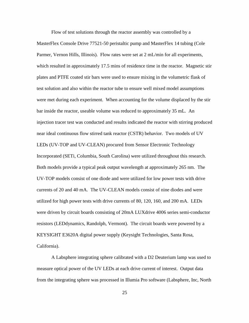
Flow of test solutions through the reactor assembly was controlled by a

MasterFlex Console Drive 77521-50 peristaltic pump and MasterFlex 14 tubing (Cole

Parmer, Vernon Hills, Illinois). Flow rates were set at 2 mL/min for all experiments,

which resulted in approximately 17.5 mins of residence time in the reactor. Magnetic stir

plates and PTFE coated stir bars were used to ensure mixing in the volumetric flask of

test solution and also within the reactor tube to ensure well mixed model assumptions

were met during each experiment. When accounting for the volume displaced by the stir

bar inside the reactor, useable volume was reduced to approximately 35 mL. An

injection tracer test was conducted and results indicated the reactor with stirring produced

near ideal continuous flow stirred tank reactor (CSTR) behavior. Two models of UV

LEDs (UV-TOP and UV-CLEAN) procured from Sensor Electronic Technology

Incorporated (SETi, Columbia, South Carolina) were utilized throughout this research.

Both models provide a typical peak output wavelength at approximately 265 nm. The

UV-TOP models consist of one diode and were utilized for low power tests with drive

currents of 20 and 40 mA. The UV-CLEAN models consist of nine diodes and were

utilized for high power tests with drive currents of 80, 120, 160, and 200 mA. LEDs

were driven by circuit boards consisting of 20mA LUXdrive 4006 series semi-conductor

resistors (LEDdynamics, Randolph, Vermont). The circuit boards were powered by a

KEYSIGHT E3620A digital power supply (Keysight Technologies, Santa Rosa,

California).

A Labsphere integrating sphere calibrated with a D2 Deuterium lamp was used to

measure optical power of the UV LEDs at each drive current of interest. Output data

from the integrating sphere was processed in Illumia Pro software (Labsphere, Inc, North

26

Sutton, New Hampshire) to acquire total power and peak wavelength data on each LED

at all drive current levels evaluated.

Figure 3 depicts the overall orientation of the reactor setup and flow scheme.

Figure 4 shows the reactor with one end cap removed to illustrate the orientation of a

magnetic stir bar and one of the LEDs within the reactor.

27

Figure 3. Schematic depicting complete experimental setup.

2

1

3

4

6

5

8

7

1. Starting Solution 2. Magnetic Stir Plate 3. Peristaltic Pump 4. LED Power Supply 5. Reactor Assembly 6. Magnetic Stir Plate 7. UV-Vis Spectrophotometer 8. Waste Container and/or HPLC/GCMS sample collection point

28

Figure 4. View of reactor endcap removed showing stir bar in middle of tube and LED at distal end.

Stir Bar

29

An Agilent Technologies Cary 60 UV-Vis spectrophotometer (Agilent

Technologies, Santa Clara, California) was used to measure the change in absorbance of

dyes over time at a peak wavelength specific to each dye as listed in

Table 1. For example, the Brilliant Blue FCF dye used in this study has a peak

wavelength at 630 nm. Over the course of an AOP experiment, reduction in absorbance

values with time at 630 nm was measured as an indicator of degradation.

The spectrophotometer was not suitable or practical in the measurement of the

achromatic chemical compounds that were weaker chromophores than the dyes (dyes are

designed to be very strong chromophores). An Agilent Technologies 6130 quadrupole

high-performance liquid chromatography (HPLC) system was used to analyze BPA via

fluorescence detector, DNT via diode array detector, and MAL via mass spectrometer.

An Agilent Technologies 7000C triple quad gas chromatography-mass spectrometry

(GCMS) system paired with an Agilent Technologies 7697A headspace sampler (Agilent

Technologies, Santa Clara, California) was used to analyze TBA and MTBE. In the case

of HPLC analyses, samples were manually collected in amber vials at predetermined time

increments during each experiment. Samples for GCMS headspace analysis were

collected manually in clear headspace vials, 1 g of sodium chloride (Thermo Fisher

Scientific, Waltham, Massachusetts) was added to each vial (to “salt out” the analyte

from solution and force it into the headspace), and the vial was immediately capped.

30

2.2.2. Experimental Procedure

Initial UV LED/ H2O2 AOP experiments were conducted to assess the

comparative differences in degradation of the 11 compounds. The solutions for all

experiments were prepared to starting concentrations of 5 mM hydrogen peroxide and

0.01 mM test compound in 250 mL of DI water. This resulted in solutions with a 500 to

1 molar ratio of H2O2 to test compound. Stock solutions were prepared at predetermined

concentrations in a base of deionized water and stored in appropriate conditions to

maintain the integrity of the solutions for use over multiple experiments. Hydrogen

peroxide procured for this research is certified at 31.9% (w/w) H2O2 content per the

certificate of analysis and was stored refrigerated at 5oC. At 5oC, the density of 31.9%

(w/w) H2O2 in water is expected to be 1.1278 g/mL. One mL of refrigerated stock H2O2

was weighed on a microbalance and compared to the certificate of analysis content. The

density of the H2O2 was used to determine a pipette volume of 126.2 microliters was

necessary to achieve the desired 5 mM concentration.

For each experiment, a precise volume of test compound stock solution was

pipetted into a 250 mL volumetric flask prefilled halfway with DI water, followed by

pipetting a precise volume of H2O2 into the flask and approximately one minute of

mixing on a vortex mixing unit. The flask was then brought to 250 mL volume with DI

water and was then capped and mixed by hand for approximately 5 minutes, a magnetic

stir bar was inserted, and the solution was further mixed on a magnetic stir plate for an

additional 15 minutes. For dye experiments, the spectrophotometer was zeroed with DI

water and set to measure absorbance values +/- 5 nm around the peak wavelength for the

31

dye being studied. Absorbance measurements were taken every one minute over a total

75 minute time period, equal to just over four reactor bed volumes to reach near steady

state final concentration. For achromatic chemicals, 2 mL samples were collected in

either amber vials or clear headspace vials at 0, 2, 4, 6, 8, 10, 12, 15, 20, 25, 30, 35, 45,

60, and 75 min increments and immediately transferred to the HPLC or GC-MS for

analysis. Initial experiments utilized the low power UV-TOP LEDs operating at 40mA to

initiate the AOP reaction.

As each experimental solution was mixing, the pump was turned on to allow for

warm up. After mixing, the pump was briefly turned off, and a 60 mL Becton Dickenson

syringe was used to load the reactor with the starting solution, the reactor stir plate was

started, and the pump was started again to initiate solution flow through the reactor (flow

was assessed at the beginning and end of each experiment to ensure the desired 2 mL/min

rate was achieved and maintained). In the case of dyes, the spectrophotometer data

collection was started simultaneous to the LED power being activated, and the

experiment was allowed to progress for 75 minutes. Five absorbance values representing

0%, 25%, 50%, 75%, and 100% starting dye concentrations were also obtained for each

experiment to generate a degradation calibration curve and assess accurate operation of

the spectrophotometer.

Subsequent experiments were conducted with various levels of UV LED drive

current. Experiments were first repeated with the lower power UV-TOP LEDs operating

at 20 mA versus the original 40mA. The higher power UV-CLEAN LEDs were then

installed in reactor end caps and experiments were repeated at 80 mA, 120 mA, 160 mA,

and 200 mA drive current. This portion was designed to assess quantum yield effect on

32

AOP optimization and hydroxyl radical production. Theoretically, higher drive current

should result in higher optical output power and, subsequently, increased hydroxyl

radical production.

Further experiments were conducted in which the molar ratio of H2O2 to test

compound was varied. Starting test compound concentrations remained constant at 0.01

mM; however, H2O2 concentrations were adjusted above and below the starting 5mM

value until optimal degradation rate or degradation extent was achieved. The starting

concentrations represented a 500:1 H2O2:test compound ratio. This ratio was then

adjusted in increments of 100:1 above and below 500:1 (e.g. 100:1, 200:1, 300:1, 400:1,

600:1, 700:1; 800:1, 900:1) to assess if a point or range of optimality exists. This was

designed to identify ratios where the reaction becomes rate limited by either inefficient

hydroxyl radical production or by potential hydroxyl radical scavenging by H2O2 when

too much H2O2 is present in solution.

Control experiments were conducted with the test compound and H2O2 solutions

mixed and passed through the reactor for a period of 75 minutes without exposure to UV

light to assess whether the specific compound is subject to degradation by reaction with

H2O2 alone. Similarly, experiments were conducted with test compound solutions

containing no H2O2 passing through the reactor with UV light exposure for a period of 75

minutes to assess whether the specific dye is subject to photodegradation by exposure to

UV light alone. It was assumed that if a compound did not show degradation at a 200

mA drive current, then optical output from lower drive currents would not cause

degradation.

33

Finally, solutions of 0.01 mM concentrations of each test compound in DI water

with no H2O2 were scanned in the spectrophotometer to determine the absorbance value

for each at the LED peak output wavelength of 265 nm. These values were then used to

calculate molar extinction coefficients and assess any impact that molar absorptivity may

have on reaction kinetics.

2.2.3. Data Analysis

Data was plotted in Microsoft Excel (Microsfot, Redmond, Washington) to show

the normalized change in effluent concentration (C/C0) of dye or chemical over time as

measured by the spectrophotometer, HPLC, or GC-MS. Absorbance values for dyes

were exported directly from the Cary 60 software, and Agilent Technologies

ChemStation software was used to integrate peaks of resultant chromatograms from the

HPLC and GC-MS analyses. The data was then modeled using the following mass

balance relationship for a completely mixed reactor with flow (Duckworth et al., 2015):

𝐶𝐶𝐶𝐶0

= 𝜏𝜏𝑘𝑘𝑆𝑆𝑒𝑒−�𝑡𝑡�𝑘𝑘𝑠𝑠+

1τ��+1

𝜏𝜏𝑘𝑘𝑆𝑆+1 (1)

Where C: concentration of dye at time t

C0: starting dye concentration at time 0

τ: residence time of solution in reactor

ks: apparent first order degradation rate constant

Residence time, τ, was computed by dividing the volume of the reactor (35 mL,

accounting for volume lost to stir bar) by the flow (2 mL/min), resulting in τ = V/Q = 17.5

34

min. An apparent degradation rate constant, ks, was calculated for each experiment using

the Microsoft Excel Solver Add-In to optimize the best overall ks that minimizes the sum

of square difference between actual and model C/C0 values. Any deviations from the

fitted model indicate deviation from CSTR conditions or deviations from first-order

reaction kinetics.

With known molar concentrations and known cuvette optical path length,

Equation 2 below was utilized to calculate the molar extinction coefficient for each

compound at the peak LED output wavelength (265 nm).

𝜀𝜀 = 𝐴𝐴𝑐𝑐𝑐𝑐

(2)

Where 𝜀𝜀: molar extinction coefficient

A: absorptivity as measured by spectrophotometer

c: concentration of species in solution

l: path length of light through solution

2.3. Results and Discussion

2.3.1. The Effect of Drive Current on Power Output

Following measurements in the integrating sphere and processing of optical

output power measurements in the Illumia Pro software, the two UV-TOP LEDs and two

UV-CLEAN LEDs with the highest total output power measurements were chosen for

installation in the reactor. Table 2 shows results of integrating sphere analysis for the

35

LEDs selected. Figure 5 shows a linear relationship (R2 = 0.9914) between applied drive

current and total additive output power for LED pairs (e.g. UV-TOP pair and UV-

CLEAN pair). A slight transition can be seen in the figure between 40 mA and 80 mA

with the change in LED models. Peak output wavelengths occurred at 265 nm and total

output power ranged from 1.31 mW at 20 mA for a UV-TOP model to 12.47 mW at 200

mA for a UV-CLEAN model.

Table 2. Output characteristics of UV LEDs utilized in reactor experiments.

LED Model Serial # Drive Current (mA)

Total Output Power (mW)

Peak Output Wavelength

(nm) UV-TOP P53 20 1.343 265

UV-TOP R54 20 1.310 265

UV-TOP P53 40 2.464 265 UV-TOP R54 40 2.442 265

UV-CLEAN U9 80 5.702 265

UV-CLEAN V5 80 5.700 265 UV-CLEAN U9 120 8.328 265

UV-CLEAN V5 120 8.340 265

UV-CLEAN U9 160 10.7 265

UV-CLEAN V5 160 10.24 265

UV-CLEAN U9 200 12.26 265

UV-CLEAN V5 200 12.47 265

36

Figure 5. Comparison of optical output power achieved from input drive current.

37

2.3.2. The Effect of Drive Current on the Removal of Organic Compounds

Figure 6 presents ks versus drive current data in a graphical format for each

compound and drive current level tested with the molar peroxide ratio at 500 mole

H2O2/mole test compound. Some degree of degradation was observed for all dyes and

achromatic chemicals under all drive current conditions. Of interest in the figure is a

linear increase in ks with increase in drive current for each compound. For example, the

ks for MAL increased from 0.144 min-1 at 20 mA drive current to 1.078 min-1 at 200 mA

drive current. The lowest ks values were associated with EB, but the linear relationship

was also observed in this case, as the ks increased linearly from 0.003 min-1 at 20 mA

drive current to 0.255 min-1 at 200 mA drive current. Exponential relationships were

observed between the drive current and degradation extent where an initial sharp linear

phase between 20 – 80 mA begins to taper, and the benefit to overall degradation extent

begins to flatten between 120 - 200 mA (Figure A1, Appendix A). If percent removal is

a priority goal over rate of removal in a real world application, such a relationship

suggests that there may not be significant added benefit in applying additional energy to

the system beyond a critical point (e.g. approximately the same percent removal may be

achieved at 120 mA when compared to 200 mA--in some cases in a comparable

timeframe). This may be particularly true of systems that are operating at or near steady

state conditions. Summary apparent first order degradation rate constants and percent

removal for all test compounds tested at all drive current levels with a molar peroxide

ratio of 500 mole H2O2/mole test compound are provided in Tables A1 and A2 and

Figures A2 through A5 (Appendix A).

38

Figure 6. Linear relationship between apparent degradation rate constant and drive current. Three example linear fits are shown.

39

These linear relationships are expected first principles of electromagnetic radiation.

However, one underlying question is if there are any phenomena occurring in the experimental

apparatus which would cause a deviation from theory—e.g., non-linear output from the LEDs

when applied in the reactor, fundamentals of hydroxyl reactions, competitive reactions, etc.

These are explored in more detail below. First, it is useful to review the theory: the energy of an

individual photon can be described by Planck’s equation:

E = hc/l (3)

Where

E: Energy (J)

h: Planck’s constant = 6.626 X 10-34 J.s

c: Speed of light = 3 X 108 m/s

l: Wavelength of light (m)

In the case of the 265 nm peak output of the LEDs utilized in this study, this results in an

energy of 7.5 X 10-19 J (or 4.68 eV) per photon. We can then use this to determine the number of

photons produced per unit time by considering the relationship to optical output power in the

following equation:

Photon production rate (photons/sec) = P/E (4)

Where

P: Optical Output Power (W)

E: Energy of a photon from Equation 3 (J)

Therefore, the optical output power is linearly related to the photon production rate,

which, in turn, generates a linear increase in hydroxyl radicals because a photon is required for

production of hydroxyl radicals from hydrogen peroxide (according to the equations on page 12)

40

and, therefore, the apparent first order degradation rate constants. The linear relationship of such

a plot can be used to predict degradation rates achievable with varying current levels. Such an

approach could be useful in fiscal decisions if implemented at full scale.

As a Watt is equivalent to a Joule/s, the units on Equation 4 become (J/s)/(J/photon) and

reduce to photons/second. Based on Equation 4, Table 3 summarizes the total number of

photons/second calculated to be produced in the reactor under each drive current level using total

output powers from Table 2. The estimated total number of photons/second increases linearly

with power output. Note that these absolute values are likely an overestimate given that the

calculations are assuming the output light is monochromatic at 265 nm. LEDs do not produce

truly monochromatic light, and 265 nm is the peak output with other neighboring wavelengths

contributing to the total output power. However, for purposes of understanding the linear nature

of the relationship between photon production rate and LED output power, assuming a single

wavelength is useful.

Table 3. Calculated photon production rate for each drive current level.

20mA 40mA 80mA 120mA 160mA

200mA

Photon production (s-1) X 1016

0.354 0.654 1.52 2.22 2.79 3.3

The theoretical linear relationship between drive current and the apparent first order

degradation rate constant also has two implications for understanding the action of the hydroxyl

radical when present in a solution containing an organic chemical, H2O2, and other hydroxyl

radicals. First, hydroxyl radicals are known to react with a wide range of constituents present in

solution (Buxton, et al. 1988). Reactions with other hydroxyl radicals are most

thermodynamically favorable because the activation energies (8 kJ/mol, Buxton, et al. 1988) that

41

are required are lower than those associated with hydroxyl-peroxide reactions (14 kJ/mol,

Buxton, et al. 1988) and common achromatic water pollutants (typically 14 - 20 kJ/mol, Buxton,

et al. 1988). As the drive current is increased, more hydroxyl radicals are produced, but this does

not lead to a disproportionate (nonlinear) proportion of hydroxyl-hydroxyl reactions. The

energetic favorability of the hydroxyl-hydroxyl radical reaction does not lead to nonlinear

relationships between power output and the apparent first order degradation rate constants. The

second implication of the linear relationships observed here is related to how hydroxyl radicals

attack organic compounds. The three oxidative modes are 1) hydrogen abstraction (i.e. removing

a hydrogen atom from a saturated hydrocarbon), 2) hydroxylation (i.e. adding the hydroxyl group

to an unsaturated hydrocarbon), or 3) oxidation without transfer of atoms. The kinetics

associated with these mechanisms are different because the shape of the pre-reactive (i.e.

transition state) complexes are different. The linear power-kinetics relationships observed in this

study (Figure 6) imply that the relative contribution of these reaction mechanisms does not

change as a function of the drive current. These two implications merit further study.

While Equations 3 and 4 relate to the relative contribution to the reaction mechanism,

they do not directly speak to the specifics of the reaction mechanism and kinetics. For example,

Erythrosine B exhibited notable behavior with respect to degradation kinetics (Figure 7). When

the drive current was 20 or 40 mA, the apparent first order degradation constants were 0.003 and

0.006 min-1 respectively, and the EB degradation curves exhibited smooth, nonlinear profiles,

consistent with first order degradation in a CSTR, and showing less than 10% total EB removal.

However, at 80 mA an interesting transition occurred wherein degradation did not appear to

reach a steady state, instead tending to continue a linear degradation pattern until the end of the

run. At 120 mA, unexpectedly unique kinetics were observed, and an inflection point appeared

42

as EB was approximately 40% degraded. After the inflection point, a secondary degradation

profile appears to begin, and degradation proceeds at a faster rate until EB is nearly 100%

degraded. Inflection points were also observed at 160 mA and 200 mA, but they were reached

more rapidly. At 200 mA, the transition at the inflection point is less pronounced as the overall

degradation proceeds at a faster rate with an apparent first order degradation rate constant of

0.255 min-1.

Rather than reflecting a deviation from the theory discussed above, these results could

suggest the presence of multiple processes relevant to degradation. Namely, Erythrosine B was

the only dye to exhibit direct photodegradation from UV light alone. Exposure at 20, 40 and 200

mA drive currents over 75 minute UV control runs resulted in 1%, 2.1% and 21 % degradation,

respectively. However, photodegradation does not completely explain the results. The

photodegradation of EB is related to its structure, but the results in Figure 7 may involve more

complex mechanisms. As noted in Table A3 and Figure A4 – A5 (Appendix A), EB has the

highest molar absorptivity at the 265 nm output wavelength of the LEDs, and it absorbs almost

5.5 times more strongly than 5 mM H2O2 at that wavelength, perhaps reducing the amount of

hydroxyl radicals available to oxidatively degrade EB. Further, there may be a change in the

relative importance of photodegradation compared to oxidative degradation as the reaction

proceeds. Initially, direct photodegradation is breaking down EB molecules, which in turn

begins to reduce the photon absorbance competition at 265 nm. Simultaneously, H2O2 molecules

benefit from this reduction in EB concentration, and hydroxyl radical production increases due to

increased photon interaction. It is possible that the inflection point marks a transition where

enough degradation has occurred and more photon energy is available for hydroxyl radical

production. At higher drive current levels, more photons are available to reach and flatten this

43

transition more rapidly. This finding led to a hypothesis that EB may benefit from greater initial

H2O2 concentrations in order to give H2O2 a higher likelihood of competing for photons in the

vicinity of the LED lens.

The literature is silent on the degradation phenomena evident in Figure 7, and pseudo-

first order kinetics have generally been utilized in different types of UV AOPs. Bairagi and

Ameta studied the degradation of EB in a UV/TiO2 reactor. Degradation values were reported in

a tabular format; however, when plotted it appears that a subtle inflection point may be present,

though the authors report pseudo-first order kinetics (Bairagi and Ameta 2016). Similarly, in a

study by Apostol et al., EB was degraded via UV/TiO2. The resultant degradation was presented

in a graphical format using overlaid spectrophotometer curves. When the approximate

absorbance values from these curves is plotted, an inflection point can be seen, though the

authors did not specifically mention the result (Apostol, et al. 2015). Though these studies

utilized TiO2, and not H2O2 as in the present study, the same competition for UV absorbance and

changes in competition over time would be expected. TiO2 requires photons to produce hydroxyl

radicals just as H2O2 does. As the EB degrades, more photons would become available to the

TiO2 substrate.

44

Figure 7. The effect of drive current on Erythrosine B removal.

45

Another deviation from theoretical behavior predicated by Equations 3 and 4 is revealed

in Figure 8, which shows removal profiles for BB, FG, and TT as a function of drive current. Of

particular interest in this figure is the transition that TT makes relative to the other dyes as the

drive current increases. Initially at 20 and 40 mA, the order of degradation rates and extents are

aligned between the dyes where the order of each follows BB > FG > TT. Overall degradation

extent for TT lags significantly at these two drive current levels as evidenced by TT degradation

extent at 40 mA being approximately equal to BB degradation extent with half the drive current

at 20 mA. At 80 mA, a transition is observed where TT begins to surpass BB and FG in overall

degradation extent, though the degradation rate is still slower. This transition continues at 120,

160, and 200 mA as TT continues to reach a greater degradation extent than BB and FG and the

degradation rates continue to move closer to parity. As with EB, Table A3 and Figure A6

(Appendix A) show that TT exhibits the second highest molar extinction at 265 nm and absorbs

3.9 times more strongly than H2O2, though it exhibited no direct photodegradation at its starting

concentration. It is likely that this non-destructive UV absorbance by TT competes with H2O2

for the available photons, and higher drive current levels begin to more rapidly mitigate this

competition as more photons are made available. Kinetics indicate that TT degradation starts out

hampered by absorbance competition resulting in a slower initial observed degradation rate and

less removal, but ultimately catches up as TT degradation proceeds and the TT absorbance

competition decreases. Comparatively, BB and FG have lower molar absorptivity at 265 nm and

tended to follow first order behavior without shifts.

46

Figure 8. The effect of drive current on the degradation of dyes.

20 mA

80 mA

200 mA

47

As compared to degradation shifts observed with TT during dye experiments, degradation

profiles for chemicals with weaker chromophores generally proceeded as expected with respect

to first order kinetics and followed the same rank order of degradation rate and extent throughout

experiments. DNT was a notable exception, where an immediate removal was observed in the

first minute of reaction under all drive current conditions. This was also true of UV control

experiments where immediate removal occurred in the first minute followed by no additional

removal over 75 minutes. Similar removal was observed in the 20 mA experiment with H2O2

where immediate removal in the first minute is subsequently followed by little removal at a slow

rate over the remainder of the experiment. Pre and post HPLC control samples ruled out any

anomalies in analysis. There appears to be a possible loss to another mechanism such as

adsorption to a component of the reactor assembly; however, adsorption would not be expected

to occur so rapidly and adsorption sites would be expected to fill over time. Experimental design

and constraints did not allow for identification of the mechanism.

MAL exhibited similar behavior in a UV control sample where there was immediate

removal followed by no removal over the remainder of a 75 minute experiment; however, MAL

exhibits a greater overall degradation rate during the AOP, and this potential loss mechanism is

masked in the other experiments. BPA exhibited 26% degradation in a UV control at 200 mA.

MTBE and TBA did not exhibit direct degradation in UV controls. TBA is a known hydroxyl

radical chain terminator and, as initially hypothesized, it was in line with DNT with the lowest

overall degradation rate and extent. TBA is also a byproduct of MTBE degradation and prior

literature suggests that the oxidation pathway of MTBE may result in 10-15% TBA formation

(Stefan, et al. 2000). It is plausible that formation and subsequent degradation of TBA during

MTBE experiments likely resulted in chain termination to a lesser extent there as well. Lower

48

comparative degradation rates and extents for DNT, TBA, and MTBE agree well with prior

published work suggesting that smaller molecules (MW < 200), in general, having electron

withdrawing substituents have lower hydroxyl radical reactivity (Lee and von Gunten 2012).

Additional supplementary plots of drive current experiments are provided in Appendix A as

Figures A8 - A30.

2.3.3. The Effect of Molar Peroxide Ratio on the Removal of Organic Compounds

Results in this section present the comparative degradation of dyes and achromatic

chemicals at varying molar ratios of H2O2 to test compound. No direct degradation from

peroxide alone was observed in control experiments for any dyes. Representative figures are

shown to demonstrate ratios where reactions were peroxide limited or where H2O2 scavenging of

hydroxyl radicals likely occurred. With one exception, optimal molar peroxide ratios for the dye

compounds did not deviate from the starting ratio of 500 moles H2O2/mole dye. There was very

little discernible difference until extreme points were reached, such as those exhibited in the

Figure 9 plot showing BB molar peroxide ratios at 100:1, 500:1, and 1000:1, where the apparent

first order degradation rate constants were 0.187, 0.476, and 0.387 min-1 for each molar peroxide

ratio, respectively. Final normalized BB concentrations for 100:1, 500:1, and 1000:1 molar

peroxide ratio experiments were 0.236, 0.068, and 0.102, respectively. The figure shows

peroxide-limited reaction at 100:1 with significantly slower degradation rate and less removal,

optimality at 500:1 with the fastest rate and largest removal, and slowed degradation rate and less

removal at 1000:1, perhaps due to radical scavenging.

Among the most interesting results in peroxide ratio experiments with the dyes are those

of EB. As hypothesized following drive current experiments, EB reaction kinetics benefited

49

significantly from increased molar peroxide ratios. Optimality was achieved at ratios in the

range of 2500-3000 moles H2O2/mole EB. Extensive peroxide ratio tests were conducted with

EB at all drive current levels with the exception of 20 mA. An especially notable point appears

in Figure 10, which shows EB molar peroxide ratio tests at 80 mA. When moving incrementally

from molar ratios of 500:1 to 3000:1, the inflection point noted during drive current experiments

gradually starts to appear and transition. Curves for higher drive currents with higher molar

peroxide ratios begin to move closer to a first order profile. Additionally, the 99% EB removal

at the end of the 3000:1 molar peroxide ratio at 80 mA surpasses the 97% removal achieved at

500:1 at 160 mA and 200 mA. The apparent first order degradation rate achieved at 3000:1

molar peroxide ratio at 80 mA (0.182 min-1) exceeds the degradation rate at 500:1 at 160 mA

(0.144 min-1) and approaches the rate of 500:1 at 200 mA (0.255 min-1) in Figure 7. A review of

the literature found no prior publications that have discovered the pronounced effect of drive

current and molar peroxide ratio on EB removal kinetics.

As with the dye compounds, no achromatic chemicals showed direct degradation from

H2O2 alone in peroxide control experiments. In general, the achromatic chemical compounds

exhibited different behavior than the dyes with regard to optimal molar peroxide ratios. TBA,

MTBE, and MAL exhibited optimal kinetics around a 100:1 peroxide ratio. MAL trials were

conducted as low as 25:1 and 50:1 ratios, and degradation rate and extent were comparable to

100:1. Comparatively, DNT and BPA were optimized in the 500:1 range, which might be

attributable to the molar extinction data exhibited in Table A3 and Figure A6 (Appendix A

illustrations). Among the chemical compounds, DNT and BPA have the highest molar

absorptivity at 265 nm and also require a higher molar peroxide ratio to optimize hydroxyl

radical production. In contrast, TBA and MTBE have the lowest molar absorptivity at 265 nm

50

with less competition for photon absorbance and were optimized at much lower peroxide

concentrations at a 100:1 ratio.

Another notable result from molar peroxide ratio experiments was observed with TBA. It

was initially hypothesized that TBA would benefit from greater peroxide ratios due to the

expected and documented chain termination mechanism and that higher concentrations of H2O2

would be required to offset the loss to that process. However, results in Figure 11 show that

likely hydroxyl radical scavenging by excess peroxide exceeds any detriment of chain

termination. Final normalized concentrations of TBA were 0.194, 0.308, and 0.439 at 100:1,

500:1, and 1000:1 molar peroxide ratios, respectively. Apparent first order degradation rates

achieved under each condition were 0.190, 0.111, and 0.067 min-1, respectively, for the 100:1,

500:1, and 1000:1 molar peroxide ratio experiments. The concentration of H2O2 used in the

100:1 molar peroxide ratio experiments is equivalent to 34 mg/L. The findings in the current

work are in agreement with a prior study on modeling and treatment system design for TBA

removal that utilized 10 – 20 mg/L H2O2 concentrations, and the authors note that at that level,

the negative effects of hydroxyl radical scavenging by excess H2O2 is not observed (Li et al,

2008). It is possible that a point of optimality below the 100:1 molar peroxide ratio used in this

study may be achievable and would require further investigation. Additional supplementary

plots of peroxide ratio experiments are provided in Appendix A as Figures A31-A45.

51

Figure 9. The effect of molar peroxide ratio on Brilliant Blue FCF removal at 200 mA.

52

Figure 10. The effect of molar peroxide ratio on Erythrosine B removal at 80 mA.

53

Figure 11. The effect of molar peroxide ratio on TBA removal at 120 mA.

54

2.3.4. Summary of the Effect of Molar Absorptivity on Chemical Removal

As alluded to above, molar light absorbance near the 265 nm LED peak output

wavelength range creates the potential for an organic compound to compete for absorbance with

H2O2 for the photons available to generate hydroxyl radicals. This is of particular interest in the

LED domain as the optical output power and resultant photon production is significantly less

than mercury lamps, as discussed previously and as shown in Tables 2 and 3. UV light can

excite the electrons present in organic chemical compounds. This is a fundamental reason why

molar absorptivity is expected to be important in water treatment applications involving UV

light. It is therefore necessary to address the role of molar absorptivity in UV LED-based AOPs.

Previous UV LED-based AOP studies have degraded chemicals with relatively high

molar extinction coefficients, but to date, there has been no previous effort to account for UV

absorbance in the interpretation or modeling of the removal profiles (Duckworth, et al. 2015;

Stewart 2016; Gallucci 2016; Mudimbi 2015; Scott, et al. 2015). However, in the current work,

accounting for molar absorptivity has helped explain the presence of inflection points observed

during EB degradation (Figure 7) and why drive current has a notable effect on the apparent first

order degradation rate constant and the degradation extent for TT (Figure 8). There is also

previously published experimental data that can be better understood by accounting for the molar

light absorbance of EB (Apostol, et al. 2015; Bairagi and Ameta 2016).

Figure A7 (Appendix A) shows a full range UV-Visible scan of all dyes (0.01 mM)

compared to H2O2 at 100:1 (1 mM) and 500:1 (5 mM) ratios. Figure A6 (Appendix A) isolates

absorbance values for each dye at the 265 nm wavelength. The molar extinction coefficient

values for all dyes and achromatic chemicals are presented in Table A3 (Appendix A) along with

absorbance ratio (background corrected to DI water) as compared to a 500:1 molar peroxide ratio

55

(e.g. molar absorptivity of test compound at 265 nm divided by molar absorptivity of 5 mM

H2O2 at 265 nm). The overall range of absorbance ratios was 0.03 to 5.45. As expected, the

dyes had a higher absorbance ratio than the achromatic chemicals. The only chemical with

notable absorbance comparable to the lowest absorbing dyes was DNT, followed by BPA. These

observations demonstrate the range of molar light absorbance that is associated with the organic

chemicals in this study.

There is also evidence to suggest that molar absorptivity at 265 nm is an important factor

in explaining deviations from CSTR model fit for individual chemicals. When plotting model

versus observed data for dyes, visual fit to the model was good for all compounds at 20 and

40mA; however, moving to 80 mA and beyond began to produce widening gaps in model fit for

some dyes. BB and FG experimental data continued to track the model relatively well, whereas

TT experimental data would notably proceed initially at a rate slower than the model predictions

and eventually cross and overshoot the model, finishing with greater than predicted degradation

extent. It is hypothesized that the deviations from model fit are again related to the molar

extinction of the dyes and the effect that the competition for absorbance has on the underlying

kinetics. The deviation at 20 and 40 mA is less significant because the reaction is more photon

limited under those conditions and impact of competing absorbance is less significant than the

overall lack of photon energy to catalyze the reaction. Table A4 (Appendix A) shows the

comparative R2 values between model and experimental data fit to Equation 1 for all dyes and

drive current levels at 500:1 peroxide ratios. Deviation from ideal model fit (where R2 = 1) is

positively correlated with higher molar absorptivity at 265 nm (e.g. model fit R2 is negatively

correlated with molar absorptivity at 265 nm). Figure 12 shows a comparison of model fit R2

versus molar absorptivity for all dyes at each drive current level. In the figure, molar

56

absorptivity values at 0.1, 0.101, 0.158, 0.169, 0.274, and 0.371 represent BB, FG, AR, SY, TT,

and EB, respectively. From a qualitative viewpoint, we observe that for 80-200 mA data series,

there is a relationship where higher R2 values are associated with lower molar absorptivity

values. In general, Figure 12 reflects a variety of complex and competing mechanisms that make

data interpretation challenging, underscoring the value and need for predictive tools.

57

Figure 12. Relationship between CSTR model fit and molar absorptivity.

58

2.4. Conclusions

This research analyzed the impact of input drive current and molar peroxide ratios on the

kinetics of UV LED-driven AOP at bench scale. There was a linear relationship between the

input drive current, optical output power, and the apparent first order degradation rate constant

for the removal of each test compound. When the drive current was 20 mA and the molar

peroxide ratio was 500 mole H2O2/mole test compound, the apparent first order degradation rate

constants were between 0.011 - 0.033 min-1 for the dyes and between 0.013 – 0.114 min-1 for

achromatic chemicals. When the drive current was 200 mA and the molar peroxide ratio was 500

mole H2O2/mole test compound, the apparent first order degradation rate constants were between

0.255 - 0.785 min-1 for the dyes and between 0.149 – 1.0748 min-1 for achromatic chemicals.

There was also a linear relationship between the drive current and the degradation extent. Data

suggested both peroxide-limited and radical-scavenged kinetics. The optimum molar peroxide

ratio for most chemicals exhibiting moderate molar absorptivity at the LED output wavelength

was at or near 500 moles H2O2/mole chemical. This observation varied at extremes where

achromatic chemicals exhibiting lower molar absorptivity were optimized at a molar peroxide

ratio of 100 moles H2O2/mole chemical and EB, with the strongest molar absorptivity, was

optimized at a molar peroxide ratio of 2500-3000 moles H2O2/mole EB. Accounting for molar

absorptivity and its photodegradation rate successfully helped to explain the molar peroxide

requirement for EB, the presence of inflection points in EB removal profiles, as well as the

relationship between drive current and the apparent first order degradation rate constants for TT

removal. The regression coefficients associated with the CSTR model fitting of data also did not

correlate well with molar absorptivity. These results are particularly notable because full scale

59

applications would involve the treatment of a variety of chemicals, each with unique light

absorbing features.

60

III. Quantitative Structure Property Relationship Models for Predicting Degradation Kinetics for a Ultraviolet Light Emitting Diode/Peroxide Advanced Oxidation Process

Keywords

QSAR, QSPR, Ultraviolet (UV), light emitting diode (LED), advanced oxidation process (AOP), hydrogen peroxide (H2O2)

Abstract

This study utilized the observed degradation kinetics of 6 dye and 5 achromatic chemical compounds in a UV-LED/H2O2 advanced oxidation process to evaluate QSPRs for predicting degradation rates. Prior to this study, QSPRs had not been evaluated for UV LED-based reactors, with published QSPRs reported for traditional mercury lamp AOP data, which has different spectral characteristics and reactor design. Overall fit to descriptors used in all of the existing QSPR models compared was relatively poor for the complete data set of compounds studied with the UV LED AOP reactor. The resultant R2 values were 0.024, 0.116, 0.157, 0.312, 0.481, and 0.864; however, several of the descriptors producing the model with the R2 of 0.864 failed to pass tests of statistical significance. When breaking the larger data set into smaller subsets of dyes and achromatic chemicals, improvement was seen with R2 values between 0.033 – 0.996, but most models and individual parameters failed tests of statistical significance. Statistical robustness was also compromised due to smaller data set sizes compared to numbers of predictors included in models. A new model was constructed for predicting the dye and achromatic chemical degradation rates utilizing zero point energy (ZPE) combined with molar absorptivity of the chemical compound at the output wavelength of the LEDs (265 nm). Overall, ZPE and molar absorptivity at 265 nm produces a QSPR model with R2 = 0.951. The model and each of the model parameters were statistically significant at a 95% confidence interval. This represents the first known use of ZPE and molar absorptivity in the construction of a QSPR model in the UV/H2O2 AOP domain.

61

3.1. Introduction

Advanced oxidation processes (AOP) using UV/H2O2 reactions have proven to be a

powerful method of generating hydroxyl radicals, which subsequently react rapidly and non-

selectively with organic compounds at near diffusion controlled rates. AOPs utilizing UV/H2O2

have proven to be highly effective at oxidizing many chemical compounds; however, the energy

requirements for UV/H2O2 AOP treatment using traditional mercury lamps has proven to be

substantially higher than other AOPs in many cases (Katsoyiannis, Canonica and von Gunten

2011). UV LEDs may be a suitable replacement for high energy consuming mercury vapor

lamps in AOPs utilizing H2O2. UV LED based water treatment is now possible; however, little

data has been available on the use of UV LED/H2O2 for the destruction of soluble organic

compounds that may threaten our water supply. Recent research at the Air Force Institute of

Technology has expanded this work to a greater number of soluble organic compounds to

improve the fundamental understanding of the AOP as it relates to LEDs.

There is also a general need to assess tools that can be used to predict chemical

degradation in UV LED-based processes. Quantitative structure-property relationships (QSPR)

can provide such a tool. The advantage of the QSPR approach, once an acceptable model is

developed, is the ability to predict removal relative to baseline conditions strictly on the basis of

the compound structure without further laboratory testing. Several previous studies have

developed QSPRs relating chemical structure to degradability (Sudhakaran, et al. 2012; Chen, et

al. 2007; Kusic, et al. 2009; Lee and von Gunten 2012; Meylan and Howard 2003; Minakata, et

al. 2009; Ohura, Amagai and Makino 2008; Sudhakaran and Amy 2013; Wang, et al. 2009; Tang

2004). QSPRs have not been evaluated for UV LED-based reactors.

62

Many existing QSPRs have been built upon degradation rate constants mined from the

literature. This approach is straightforward as there is no time or cost associated with conducting

experiments; however, there is no control over the quality of the underlying experiments from

which the kinetic data was derived. Furthermore, experimental conditions (batch vs CSTR,

varying reactant concentrations, varying UV light sources, varying retention times, etc) under

which the rate constants were measured are often very disparate. There is risk in using large,

low quality data sets, as they may offer a misleading impression with respect to the relative

importance of model parameters. The present study sought to investigate the use of a smaller,

high quality data set built from degradation experiments of 6 dye and 5 weaker chromophore

compounds tested in the same bench-scale UV LED reactor under identical operating conditions.

Apparent first order degradation rate constants for the 11 compounds were used to investigate

molecular descriptors that are most significant to the UV LED-based AOP by first assessing

significance of molecular descriptors used in existing QSPRs developed with traditional mercury

lamp AOP data and then using multiple linear regression (MLR) to assess potential new QSPR

models.

3.1.1. Overview of QSPR and Molecular Descriptors

Quantitative structure-property relationship (QSPR) models seek to relate structural

features of a chemical compound to physicochemical activity (Yee and Wei 2012). Fundamental

to the successful development and application of QSPR models is the selection of molecular

descriptors (MD) that adequately represent the important parameters affecting the observed

property of interest. QSPR methods have been used historically in the design of pharmaceuticals

that target specific diseases or medical conditions; however, use of the methodology for

63

prediction in environmental applications has increased significantly in recent decades (Singh, et

al. 2014). MDs are numerous and diverse with various software packages capable of calculating

anywhere from 200 to over 3000 unique descriptors for a single chemical compound (Hong, et

al. 2012). There is an art and a science to selecting the most important subset of MDs relevant to

the goals and mechanisms of each study. Doing so can improve prediction accuracy, facilitate

interpretation of a model, and prevent potential over-fitting of data (Singh and Gupta 2014).

In general, MDs are classified into five categories: 1) physicochemical (e.g. octanol-

water partition coefficient, Log P, density, melting point, half-life in water/air, persistence time),

2) constitutional (e.g. numbers of atoms and bonds, molecular weight, hydrogen percent, carbon

percent, hydrogen bond donors, hydrogen bond acceptors, etc.), 3) geometrical (e.g. maximum

Z-length, molecule surface area, etc.), 4) topological (e.g. connectivity and valence connectivity

indexes, etc.), and 5) quantum-chemical (polarizability, electric dipole moment, total energy,

electron density, etc) (Servien, et al. 2014; Singh, et al. 2013). Numerous software packages are

available for the calculation of MDs, with some specializing only in subsets of these categories.

Options range from freeware to commercial software packages, and capabilities range from

calculating hundreds of descriptors to several thousand descriptors, depending on the software

selected.

3.1.2 Use of QSPR and Molecular Descriptors in AOPs and Similar Domains

QSPRs have been utilized to predict degradation rates in numerous environmental

applications including atmospheric reactions, direct UV photolysis in aqueous and non-aqueous

solutions, and reactions in AOPs used for water treatment. Methodology and descriptor selection

varies broadly. One study focused on developing a QSPR to model the removal of organic

micropollutants (primarily pharmaceuticals, personal care products, and pesticides) in four

64

different river water sources (Colorado River, Passaic River, Ohio River, and Suwannee

synthetic water) via ozonation AOP. QSPR models were built using bench scale data from

experiments with the source waters. An initial set of 40 molecular descriptors potentially

influencing AOP were selected using MLR and ranged from simple atom counts to complex

quantum-chemical properties. An artificial neural network (ANN) was created with a

compilation of molecular descriptors of pollutants from the four water sources. The ANN

identified the following relevant molecular descriptors for inclusion in QSPR models: LUMO–

HOMO energy difference, electron affinity, number of halogen atoms, number of ring atoms,

weakly polar component of the solvent accessible surface area, and oxygen to carbon ratio

(Sudhakaran, et al. 2012). The same research group used a different approach in developing

additional QSPRs using ozone and hydroxyl radical degradation rate constants as dependent

variables. Molecular descriptors selected were double bond equivalence, ionization potential,

electron affinity, and weakly-polar component of solvent accessible surface area. As opposed to

ANN used to construct the prior QSPR models, MLR was used to build the additional models

(Sudhakaran and Amy 2013). In both cases, models were validated with internal and external

data sets and showed high goodness of fit.

In another study related to hydroxyl radical reactions in water, a QSPR was built using

MLR on quantum chemical descriptors to predict degradation rate constants. The molecular

descriptors found to be significant were the HOMO energy, average net H atom atomic charges,

molecular surface area (MSA), and dipole moment. Degradation rate constants were positively

correlated with increasing HOMO energy and molecular surface area and negatively correlated

with increasing H atom atomic charge and dipole moment. Particular emphasis was placed on

following QSPR development guidelines set forth by the Organization for Economic

65

Cooperation and Development (OECD; http://www.oecd.org/env/ehs/oecdquantitativestructure-

activityrelationshipsprojectqsars.htm), including validation, domain of applicability, and

mechanistic interpretation. (Wang, et al. 2009)

A similar methodology was used to develop a QSPR to predict hydroxyl radical

degradation rate constants for 78 aromatic compounds in water. A genetic algorithm (heuristic

method) was used to select relevant descriptors and multiple linear regression was used to build

the QSPR models. The DRAGON software package was used to calculate molecular

descriptors. A final model consisting of 4 molecular descriptors (HOMO, molecular path count

of order 8, Geary auto-correlation-2/lag weighted by polarizabilities, leverage weighted

autocorrelation of lag 7/weighted by atomic polarizabilities) was found to be ideal without

overfitting and HOMO energy was the main contributor to the resultant degradation rate. (Kusic,

et al. 2009)

Jin et al. developed a QSPR model for the prediction of hydroxyl radical degradation

rates for emerging micro pollutants. The model building data set included 118 emerging micro

pollutants, including some from the literature and some experimentally collected. DRAGON

was used to calculate 951 descriptors. MLR was used to build and refine a final model which

includes the mean atomic Sanderson electronegativity, the number of double bonds, the number

of primary alkyl halide functional groups, number of hydrogen bond acceptors, Moran

autocorrelation of lag 2 weighted by mass, Balaban V index, and signal 27 weighted by

polarizability. (Jin, et al. 2015)

Huang et al. built a QSPR model based on ten sulfonamide compounds (SAs) degraded in

TiO2 photocatalytic systems. Partial least squares regression was used to build optimal QSAR

models. Degradation of SAs was found to be strongly related to the highest occupied molecular

http://www.oecd.org/env/ehs/oecdquantitativestructure-activityrelationshipsprojectqsars.htm

http://www.oecd.org/env/ehs/oecdquantitativestructure-activityrelationshipsprojectqsars.htm

66

orbital, the maximum values of nucleophilic attack (f(+)x), and the minimum values of the most

negative partial charge on a main-chain atom (q(C)min). (Huang, et al. 2015)

Borhani et al. developed a QSPR for predicting the hydroxyl radical rate constant for a

dataset of 457 water contaminants spanning 27 chemical classes. A constricted binary particle

swarm optimization and MLR (BPSO-MLR) technique was used to fit an optimal model with

eight molecular descriptors including sphericity, R autocorrelation of lag 1/unweighted, Broto-

Moreau autocorrelation of a topological - lag 2/weighted by atomic van der Waals volumes,

highest eigenvalue of Burden matrix/weighted by atomic Sanderson electronegativities, spectral

moment 05 from edge adjacent matrix weighted by edge degrees, number of terminal primary C,

number of aromatic hydroxyls, and number of sulfur atoms. (Borhani, et al. 2016)

Tang investigated the use of LUMO as a sole descriptor in a predictive model for

degradation in a UV/H2O2 AOP. The descriptor produced models with strong R2 values ranging

from 0.9094 – 0.9876 for separate chemical classes of alkane, benzene, halide, and phenol

compounds. Separate models were built for each chemical class with only n=3 compounds

employed in each model. Each class resulted in vastly different coefficients and a model with all

classes combined would have likely resulted in a poor model fit. LUMO showed less fit to

individual models built with alkenes, aromatic hydrocarbons, carboxylic acids, and sulfonic acids

with lower R2 values ranging from 0.06 – 0.77. (Tang 2004)

Additional QSPR models have been developed for predicting degradation rates for the

direct photodegradation of compounds in either aqueous or non-aqueous solutions. One such

model was built to predict degradation of polybrominated diphenyl ethers in water/methanol or

methanol solutions. Partial least squares regression was used to build the model and the

following descriptors were found to be significant: LUMO–HOMO energy gap, most positive

67

Mulliken atomic charges on a hydrogen atom, log k, molecular weight, average molecular

polarizability, and average Mulliken atomic charges on bromine atoms (Chen, et al. 2007).

Other QSPRs have been built to predict photodegradation of compounds on aerosol surfaces

(Ohura, et al. 2008) and oxidation of compounds in the atmosphere (Meylan and Howard 2003)

using similar model building techniques.

A different model building technique employed by Minakata et al. involved the

development of a group contribution method (GCM) to predict hydroxyl radical degradation rate

constants by predicting rate constants for individual reaction mechanisms: 1) hydrogen

abstraction, 2) hydroxyl radical addition to alkenes, 3) hydroxyl radical addition to aromatic

compounds, and 4) hydroxyl radical interaction with compounds containing sulfur, nitrogen, or

phosphorus. The GCM is predicated on the idea that the experimental degradation rate constant

for a given organic compound is the combined rate of all elementary hydroxyl radical reactions.

A total of 66 group rate constants and 80 group contribution factors are included in the GCM.

Degradation rate constants were mined from the literature with 310 compounds used for

calibration and 124 compounds used for prediction. Genetic algorithms were used to determine

the group rate constants and contribution factors. The best results for calibrations and

predictions were within 0.5-2 times experimental values. (Minakata, et al. 2009) Though the

GCM is a robust methodology, it also requires a large data set for proper calibration and

prediction (Minakata, et al. 2014).

68

3.2. Materials and Methods

3.2.1 Data Set and Generation of Molecular Descriptors

A set of experimental data (including observed degradation rate constants, degradation

extent, and molar absorptivity values) was collected as previously described for 6 dye and 5

achromatic chemical compounds studied in a UV LED/H2O2 AOP reactor described in Chapter

2. The scope of the data set and associated degradation rate constants are constrained to the

specific reactor and associated reactor parameters utilized in the experiments (e.g. flow, volume,

chemical concentrations, UV intensity, etc.). Experimental procedures such as competition

kinetics were not utilized to link the apparent first order degradation rate constants to second

order hydroxyl radical rate constants commonly reported in the literature.

A freeware package from the US Food and Drug Administration called MOLD2 was used

to generate 777 molecular descriptors for each test compound (US Food and Drug

Administration 2015). MOLD2 requires loading of a structure data file (SDF) for each

compound and performs computations based on parameters contained in the SDF. The requisite

SDF for each compound was available and was downloaded from the National Institutes of

Health PubChem data repository (National Institutes of Health 2016). Additional chemical

properties were also selected for each dye and chemical from information published directly on

the PubChem website (National Institutes of Health 2016). As MOLD2 does not have quantum

chemistry capabilities, two additional software packages were used to produce those descriptors,

MOPAC (Stuart Computational Chemistry 2016) and Spartan ’16 (Wavefunction 2017). In

order to use MOPAC, the SDFs from PubChem had to be converted to MOPAC format (.mop).

This was completed in open source software called Babel (O'Boyle, et al. 2011) that converts

descriptor input files across multiple computational platforms. Conversions were completed for

69

all compounds and quantum values were successfully computed in MOPAC. Spartan software

also requires input files specifically formatted for the platform; however, it can directly import

SDF files and convert them internally. Several of the chemical compound structures were

available in a Spartan database, whereas dye molecules were imported and manually verified for

structural accuracy following conversion from 2D to 3D format. A full listing of MOLD2 and

PubChem descriptors is provided in Appendix B.

3.2.2. QSPR Model Development

The JMP statistical software package was used to test multivariate QSPR model

candidates through linear regression by regressing degradation rate constants on one or more

molecular descriptors. Regression techniques are among the most popular methods in the

literature and a basic model takes the form of Equation 5:

𝑦𝑦𝑖𝑖 = 𝛽𝛽0 + 𝛽𝛽1𝑥𝑥𝑖𝑖1 + 𝛽𝛽2𝑥𝑥𝑖𝑖2 + ⋯+ 𝛽𝛽𝑛𝑛𝑥𝑥𝑖𝑖𝑛𝑛 + 𝜀𝜀𝑖𝑖 (5)

Where

𝑦𝑦𝑖𝑖: property being predicted (degradation rate constant in this case)

𝛽𝛽0: constant

𝛽𝛽1, 𝛽𝛽2,⋯ ,𝛽𝛽𝑛𝑛: regression coefficients

𝑥𝑥𝑖𝑖1, 𝑥𝑥𝑖𝑖2, ⋯, 𝑥𝑥𝑖𝑖𝑛𝑛: predictor variables of compound i (molecular descriptors in this case)

Two approaches were taken to QSPR model development. In the first approach, relevant

models and their associated descriptors were mined from the literature. QSPR models from the

literature predicting hydroxyl radical rate constants cannot be compared directly due to the

limitations noted in Section 3.2.1; however, the molecular descriptors utilized in building those

models are certainly relevant for comparison and tests of statistical significance. Models were

70

built using the same descriptors or comparable descriptors employed in models discussed

(summarized in Table 4) and standard least squares regression was used to fit the best possible

model with those descriptors. In the second approach, MLR was used to build new models from

the descriptors calculated, as described in Section 3.2.1. A stepwise procedure was used to

down-select the descriptors by which variables are added to the model one at a time until the

descriptor with the best fit (R2) is found. The procedure then moves forward to find the next

descriptor that continues to improve the R2 when added to the model. The p-value threshold

stopping rule was used with default probability to enter and exit of 0.25 and 0.1, respectively.

Because the overall data set is small (6 dyes and 5 achromatic chemicals), caution was taken not

to include more than 1-2 descriptors in final models in order to avoid overfitting. Assessment of

model fit was completed by evaluating coefficient of determination (R2), adjusted R2 (R2adj), root

mean square error (RMSE), Fisher criterion (F), standard error of the estimate (SE), and p-value

tests for significance of predictors. Evaluation of R2adj is of particular interest as it accounts for

the inclusion of additional predictors and compares the improvement that inclusion of an

individual predictor has on model fit to the improvement that would be expected by chance.

71

Table 4. Molecular descriptors utilized in QSPRs built from traditional mercury lamp AOP data.

QSPR Model/Reference Descriptors Used Parameters/Notes 1. Wang, et al. 2009 model - EHOMO (HOMO)

- Avg net atomic charges on H (QH) - Molecular surface area (MSA) - Dipole Moment (DM)

Domain of applicability for original model was phenols, alkanes, and alcohols. Unable to obtain QH values with MOPAC/Spartan/MOLD2.

2. Jin, et al 2015 model - Mean atomic Sanderson negativity - # double bonds (DB) - # primary alkyl halides (nCH2RX) - # hydrogen acceptors (HA) - # Moran autocorrelation lag 2 weighted by mass (MATS2m) - Balaban V index (BV) - Signal 27 weighted by polarizability (Mor27p)

Applied to a large data set of micro pollutants. Unable to obtain Mor27p values with MOPAC/Spartan/MOLD2.

3. Tang 2004 model ELUMO (LUMO) Applied to alkane, benzene, halide, and phenol classes

4. Kusic, et al. 2009 model - HOMO - Molecular path count of order 8 - Geary autocorrelation of lag 2/weighted by polarizabilities - Leverage weighted autocorrelation lag 7/weighted by polarizabilities

Found EHOMO to be the main contributor.

5. Sudhakaran and Amy 2012 model

- HOMO-LUMO energy gap - Electron affinity (EA) - # halogen atoms - # ring atoms - Weakly polarizable surface (WPSA) - Oxygen to carbon ratio (OtoC)

Electron affinity and WPSA not available in MOPAC/Spartan/MOLD2. Negative of the LUMO approximates electron affinity.

6. Sudhakaran and Amy 2013 model

- Double bond equivalence (DBE) - Weakly polarizable surface area (WPSA) - Ionization potential (IP) - Electron affinity (EA)

Electron affinity and WPSA not available in MOPAC/Spartan/MOLD2. Negative of the LUMO approximates electron affinity. Negative of the HOMO approximates ionization potential.

72

3.3. Results and Discussion

3.3.1. Assessment of Existing QPSR Models

Three models were built with each set of descriptors from Table 1 using a combined data

set of dyes and achromatic chemicals (n=11), a data set of dyes alone (n=6), and a data set of

achromatic chemicals alone (n=5). The rationale for this approach is to assess domains of

applicability as the dye structures in general are much larger, more complex, and contain

different atoms and functional groups than the achromatic chemicals. A summary of parameter

estimates and statistics is provided in Table A5 (Appendix A).

3.3.1.1. Wang, et al. 2009 Model

As noted in Table 4, the Wang, et al. model consisted of 4 molecular descriptors. Three

of the descriptors (energy of the highest occupied molecular orbital (HOMO), molecular surface

area (MSA), and dipole moment (DM)) were available in the software packages used in this

study; however, average net atomic charges on H could not be obtained directly. When

evaluating the three available descriptors using MLR and putting in the form of Equation 1, the

following model was obtained.

Kpred = 1.4985277 + 0.120925(HOMO) + 0.0009508 (MSA) – 0.023057 (DM)

Overall, the model is a poor fit to the full n=11 data set as evidenced by weak R2 and

R2adj values of 0.157 and -0.204, respectively. Figure 13 presents a plot of measured versus

predicted apparent first order degradation rate constants. The solid line represents ideal fit where

kpred/kmeas = 1. Thinner dashed lines demark regions where kpred/kmeas values are less than 0.5 or

greater than 2. Similar plots are provided for all remaining model evaluations. Tests of

significance fail for the full model and all individual parameters.

73

When looking at the data set of n=6 dyes alone, the fit of the model begins to shift with

R2 of 0.801; however, the R2adj value remains low at 0.50, indicating likelihood of chance

parameter fit (Figure 14). Lack of statistical significance remains evident in the full model and

all parameters. The resultant model is as follows.

Kpred = -4.029688 - 0.596527(HOMO) - 0.001318 (MSA) + 0.0351431 (DM)

The data set of n=5 achromatic chemicals shows significant improvement in model fit in

terms of both R2 and R2adj and results in the model below. The overall R2 fit improves to 0.983,

whereas R2adj is 0.933 (Figure 15). However, tests of statistical significance continue to fail for

the full model and all individual parameters.

Kpred = 22.060342 + 2.2074904(HOMO) - 0.020181 (MSA) + 0.5241355 (DM)

Overall results indicate that these three molecular descriptors together may be useful in

predicting the degradation of the achromatic chemical compounds as evidenced by the high

adjusted coefficient of determination; however, caution should be taken given the lack of

statistical significance in conjunction with the small data set size. The descriptors are also

predictive to a lesser extent for the dye compounds. When grouping the dyes and achromatic

chemicals into a combined data set, it is evident that there are structural diversities that likely

shift the domain of applicability of the QSPR.

74

Figure 13. Actual versus predicted degradation rate constants utilizing Wang et al. descriptors with the full data set.

75

Figure 14. Actual versus predicted degradation rate constants utilizing Wang et al. descriptors with the dye data set.

76

Figure 15. Actual versus predicted degradation rate constants utilizing Wang et al. descriptors with the achromatic chemical data set.

77

3.3.1.2. Jin, et al. 2015 Model

The Jin, et al. model consists of 7 molecular descriptors, including mean atomic

Sanderson negativity (MASN), number of double bonds (DB), number of primary alkyl halides

(CH2RX), number of hydrogen bond acceptors (HBA), Moran autocorrelation lag 2 weighted by

mass (MAL2m), Balaban V index (BV), and signal 27 weighted by polarizability (Mor27p). Six

of the seven descriptors were able to be produced; however, Mor27p was not directly available in

the software packages utilized. The model below produced with the full n=11 data set results in

a weak coefficient of determination of 0.481 and even weaker R2adj of -0.297 (Figure 16). The

full model and all parameters failed tests of statistical significance.

Kpred = 6.2253693 + 0.2855091(HBA) – 1.433525(BV) – 0.247911(DB) – 5.817407(MASN) – 0.565174(MAL2m) – 0.076636(CH2RX)

Fitting these parameters to n=6 dyes alone or n=5 achromatic chemicals alone is not

possible due to degrees of freedom violation and bias in the model caused by the comparatively

large number of descriptors. Overfitting is apparent and the resultant R2 is 1 in both cases. Jin et

al. found that the Balaban V index and the number of hydrogen bond acceptors showed the best

correlation to the degradation rate constant in their model. When using only those two

descriptors, no better model fit can be obtained with the full data set or data subsets. We can

conclude that the Jin, et al. descriptors do not fit the dye and chemical data set used in this study.

78

Figure 16. Actual versus predicted degradation rate constants utilizing Jin et al. descriptors with the full data set.

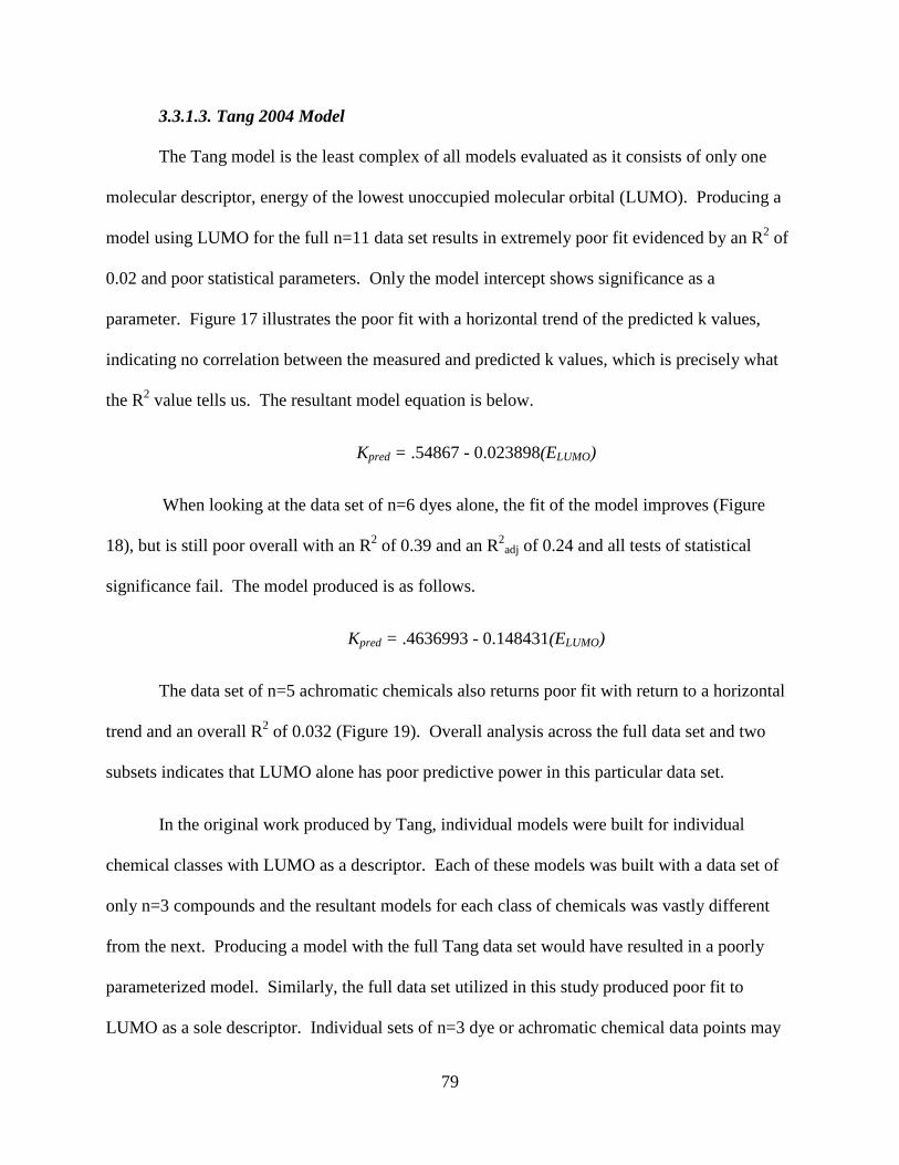
79

3.3.1.3. Tang 2004 Model

The Tang model is the least complex of all models evaluated as it consists of only one

molecular descriptor, energy of the lowest unoccupied molecular orbital (LUMO). Producing a

model using LUMO for the full n=11 data set results in extremely poor fit evidenced by an R2 of

0.02 and poor statistical parameters. Only the model intercept shows significance as a

parameter. Figure 17 illustrates the poor fit with a horizontal trend of the predicted k values,

indicating no correlation between the measured and predicted k values, which is precisely what

the R2 value tells us. The resultant model equation is below.

Kpred = .54867 - 0.023898(ELUMO)

When looking at the data set of n=6 dyes alone, the fit of the model improves (Figure

18), but is still poor overall with an R2 of 0.39 and an R2adj of 0.24 and all tests of statistical

significance fail. The model produced is as follows.

Kpred = .4636993 - 0.148431(ELUMO)

The data set of n=5 achromatic chemicals also returns poor fit with return to a horizontal

trend and an overall R2 of 0.032 (Figure 19). Overall analysis across the full data set and two

subsets indicates that LUMO alone has poor predictive power in this particular data set.

In the original work produced by Tang, individual models were built for individual

chemical classes with LUMO as a descriptor. Each of these models was built with a data set of

only n=3 compounds and the resultant models for each class of chemicals was vastly different

from the next. Producing a model with the full Tang data set would have resulted in a poorly

parameterized model. Similarly, the full data set utilized in this study produced poor fit to

LUMO as a sole descriptor. Individual sets of n=3 dye or achromatic chemical data points may

80

have produced models of good fit, but such small data sets produce results with poor statistical

relevance.

81

Figure 17. Actual versus predicted degradation rate constants utilizing Tang descriptors with the full data set.

82

Figure 18. Actual versus predicted degradation rate constants utilizing Tang descriptors with the dye data set.

83

Figure 19. Actual versus predicted degradation rate constants utilizing Tang descriptors with the achromatic chemical data set.

84

3.3.1.4. Kusic, et al. 2009 Model

The Kusic, et al. model consists of 4 molecular descriptors including EHOMO, molecular

path count of order 8 (PC8), Geary autocorrelation of lag 2/weighted by polarizabilities

(GACL2wP), and autocorrelation lag 7/weighted by polarizabilities (AL7wP). All the

descriptors were reproducible in this study. The full n=11 data set produces a poor model fit

with R2 of 0.311 and R2adj of -0.147.

Kpred = 5.5068128 + 0.4620056(EHOMO) – 0.001947(AL7wP) – 0.760255(GACL2wP) – 0.009211(PC8)

When reviewing the plot of actual versus predicted k (Figure 20), the two data points

representing malathion and Allura Red AC deviate from the trend followed by the remaining

data points. In general, it is not good practice to remove data points unless there is sound

reasoning for why outliers may exist. In this case, we would review the structures and assess the

domain of applicability of the two outliers. In the case of malathion, it is unique in that it is the

only compound that contains phosphorous. However, there are no immediate differences that

can be discerned for Allura Red AC; it is an azo dye just as Sunset Yellow FCF and Tartrazine

and has a similar molecular structure. In principle, there is no immediately obvious reason to

remove Allura Red AC; however, it is interesting to remove both compounds to assess the

impact on model fit. With reduction to a data set of n=9, model fit is substantially enhanced

(Figure 21) to an R2 of 0.985 and R2adj of 0.971 with the following resultant model. The full

model and all parameters are also statistically significant.


85

The data set of n=6 dyes alone (including return of Allura Red to the set) produces strong

model fit as observed by R2 of 0.992 and R2adj of 0.961 (Figure 22); however, in contrast to the

prior model, the full model and all parameters fail tests of statistical significance. The resultant

model is as follows.


The set of n=5 achromatic chemicals cannot produce a model without bias due to number

of data points versus predictors. In general, descriptors utilized by Kusic, et al. may be useful in

predicting the observed degradation rates of dyes; however, we must be cautious of the potential

for overfitting with the small sample size and lack of statistical significance. The descriptors

may also be useful to the overall data set if we have valid reason to exclude one dye and one

achromatic chemical as outliers, though there is no immediately apparent reason to do so.

86

Figure 20. Actual versus predicted degradation rate constants utilizing Kusic et al. descriptors with the full data set.

87

Figure 21. Actual versus predicted degradation rate constants utilizing Kusic et al. descriptors and omitting malathion and Allura Red AC.

88

Figure 22. Actual versus predicted degradation rate constants utilizing Kusic et al. descriptors with the dye data set.

89

3.3.1.5. Sudhakaran and Amy 2012 Model

The first set of Sudhakaran and Amy descriptors consists of the HOMO-LUMO energy

gap, electron affinity (EA), number of halogen atoms, number of ring atoms, weakly polarizable

component of the solvent accessible surface area (WPSA), and oxygen to carbon ratio (OtoC).

There was no direct method for obtaining WPSA in the software utilized in this study, but the

remainder were obtained directly or through mathematical manipulation of existing descriptors.

The descriptors fit to the full n=11 data set results in an R2 of 0.86 and R2adj of 0.72 (Figure 23).

Statistical parameters show mixed results. The overall model is statistically significant;

however, the individual parameters of “Halogen” and “OtoC” fail to pass the p-value test.

Kpred = 7.0584708 – 0.57937(EA) + 0.6832793(HOMO-LUMO) – 0.09306(Halogen) - 0.063115(Ring Atoms) – 0.0192175(OtoC)

Parameter estimates for subsets of dyes and achromatic chemicals alone cannot be

obtained due to bias caused by the number of predictors (e.g. more predictors than data points).

Overall analysis indicates that this model is likely not a good fit to this data set and results in a

coefficient of determination that is likely due primarily to chance overfitting as evidenced by the

lower R2adj.

90

Figure 23. Actual versus predicted degradation rate constants utilizing Sudhakaran and Amy, 2012 descriptors with the full data set.

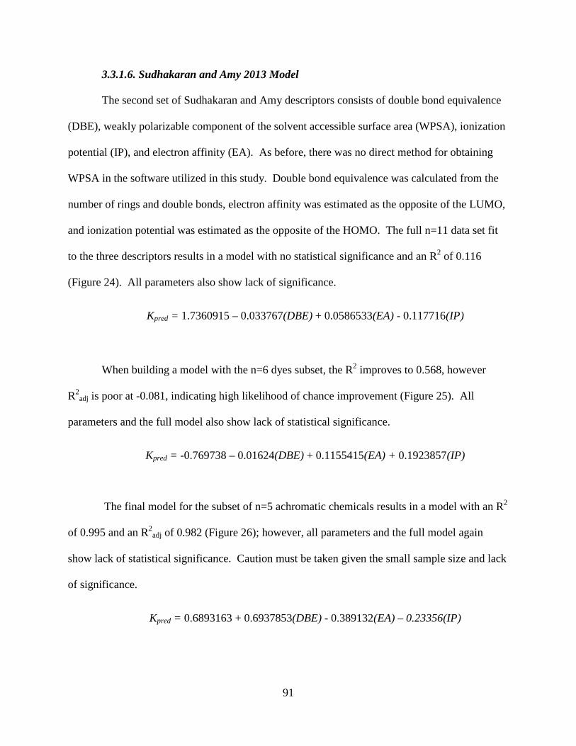
91

3.3.1.6. Sudhakaran and Amy 2013 Model

The second set of Sudhakaran and Amy descriptors consists of double bond equivalence

(DBE), weakly polarizable component of the solvent accessible surface area (WPSA), ionization

potential (IP), and electron affinity (EA). As before, there was no direct method for obtaining

WPSA in the software utilized in this study. Double bond equivalence was calculated from the

number of rings and double bonds, electron affinity was estimated as the opposite of the LUMO,

and ionization potential was estimated as the opposite of the HOMO. The full n=11 data set fit

to the three descriptors results in a model with no statistical significance and an R2 of 0.116

(Figure 24). All parameters also show lack of significance.

Kpred = 1.7360915 – 0.033767(DBE) + 0.0586533(EA) - 0.117716(IP)

When building a model with the n=6 dyes subset, the R2 improves to 0.568, however

R2adj is poor at -0.081, indicating high likelihood of chance improvement (Figure 25). All

parameters and the full model also show lack of statistical significance.

Kpred = -0.769738 – 0.01624(DBE) + 0.1155415(EA) + 0.1923857(IP)

The final model for the subset of n=5 achromatic chemicals results in a model with an R2

of 0.995 and an R2adj of 0.982 (Figure 26); however, all parameters and the full model again

show lack of statistical significance. Caution must be taken given the small sample size and lack

of significance.

Kpred = 0.6893163 + 0.6937853(DBE) - 0.389132(EA) – 0.23356(IP)

92

Figure 24. Actual versus predicted degradation rate constants utilizing Sudhakaran and Amy, 2013 descriptors with the full data set.

93

Figure 25. Actual versus predicted degradation rate constants utilizing Sudhakaran and Amy, 2013 descriptors with the dye data set.

94

Figure 26. Actual versus predicted degradation rate constants utilizing Sudhakaran and Amy, 2013 descriptors with the achromatic chemical data set.

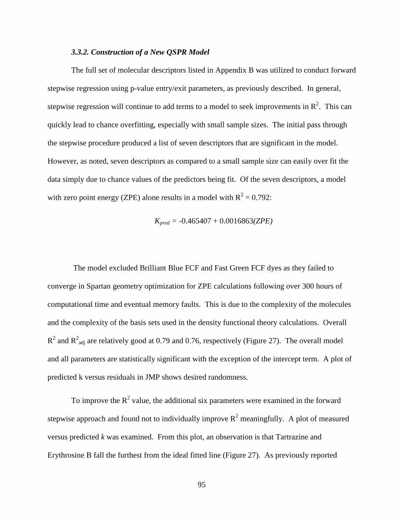
95

3.3.2. Construction of a New QSPR Model

The full set of molecular descriptors listed in Appendix B was utilized to conduct forward

stepwise regression using p-value entry/exit parameters, as previously described. In general,

stepwise regression will continue to add terms to a model to seek improvements in R2. This can

quickly lead to chance overfitting, especially with small sample sizes. The initial pass through

the stepwise procedure produced a list of seven descriptors that are significant in the model.

However, as noted, seven descriptors as compared to a small sample size can easily over fit the

data simply due to chance values of the predictors being fit. Of the seven descriptors, a model

with zero point energy (ZPE) alone results in a model with R2 = 0.792:

Kpred = -0.465407 + 0.0016863(ZPE)

The model excluded Brilliant Blue FCF and Fast Green FCF dyes as they failed to

converge in Spartan geometry optimization for ZPE calculations following over 300 hours of

computational time and eventual memory faults. This is due to the complexity of the molecules

and the complexity of the basis sets used in the density functional theory calculations. Overall

R2 and R2adj are relatively good at 0.79 and 0.76, respectively (Figure 27). The overall model

and all parameters are statistically significant with the exception of the intercept term. A plot of

predicted k versus residuals in JMP shows desired randomness.

To improve the R2 value, the additional six parameters were examined in the forward

stepwise approach and found not to individually improve R2 meaningfully. A plot of measured

versus predicted k was examined. From this plot, an observation is that Tartrazine and

Erythrosine B fall the furthest from the ideal fitted line (Figure 27). As previously reported

96

elsewhere (Chapter 2), those two dyes in particular showed a high molar absorptivity at the 265

nm wavelength (the peak output wavelength of the LEDs being used in the study), and it was

hypothesized elsewhere (Chapter 2) that competition with H2O2 for UV absorbance likely

affected the kinetics of the AOP. Absorbance at 265 nm was added as a predictor to the model to

see what effect it may have. Adding the term tightens the model significantly, resulting in R2

and R2adj values of 0.951 and 0.934, respectively, and the full model and all parameters show

significance (Table 5 and Figure 28). A predicted k versus residual plot produced in JMP also

shows randomness with no pattern, as desired. The resultant model and associated parameters

are as follows.

Kpred = -0.404717 + 0.0018182(ZPE) – 1.093331(Abs265)

3.3.3. Physical significance of newly constructed QSPR model

Parameters in the model show a positive correlation between degradation rate and ZPE

and a negative correlation between degradation rate and absorbance at 265. The ZPE is a value

that comes from thermodynamic calculations in Spartan. Both of these correlations make

intuitive sense when considering reaction kinetics. The theory behind ZPE is that even at 0

degrees Kelvin, molecules will still have some level of vibrational energy.

This represents the first known use of ZPE in a QSPR model; however, larger data sets

should be tested to further assess the utility of this novel parameter. It was hypothesized in

Chapter 1 that descriptors related to frontier electron density, particularly HOMO, would be

significant model parameters. This was not the case, as models incorporating HOMO, LUMO,

and HOMO-LUMO performed relatively poorly and ZPE emerged as an important descriptor for

this data set.

97

Table 5. Parameters and tests of statistical significance for new models built with zero point energy and molar absorptivity.

Model Data Set Rsquare Rsquare Adj RMSE F Ratio Prob > F Parameter Parameter Estimate Prob > tNew Model with ZPE Omit BB and FG (n=9) 0.792 0.762 0.169 26.63 0.0013 Intercept -0.465407 0.0572

ZPE 0.0016863 0.0013

New Model with ZPE and Abs Omit BB and FG (n=9) 0.951 0.935 0.089 58.3 0.0001 Intercept -0.404717 0.0096ZPE 0.0018182 <0.0001Abs265 -1.093331 0.0045

98

Figure 27. Actual versus predicted degradation rate constants utilizing Zero Point Energy as a descriptor with the full data set.

99

Figure 28. Actual versus predicted degradation rate constants utilizing Zero Point Energy and molar absorptivity as descriptors with the full data set.

100

3.4. Conclusions

This study sought to utilize a small, high quality data set of the observed degradation

kinetics of 6 dye and 5 achromatic chemical compounds tested in a bench-scale UV LED reactor

to compare fit with molecular descriptors in published QSPRs developed with traditional

mercury lamp AOP data and also to use MLR methodology to construct a new QSPR model.

Prior to this study, QSPRs had not been evaluated for UV LED-based reactors. Overall fit to

descriptors used in all the existing QSPR models compared was relatively poor for the overall

data set of dyes and achromatic chemicals combined. The resultant R2 values were 0.024, 0.116,

0.157, 0.312, 0.481, and 0.864; however, several of the descriptors producing the model with the

highest R2 of 0.864 failed to pass tests of statistical significance. When breaking the larger data

set into smaller subsets of dyes and achromatic chemicals, improvement was seen with R2 values

between 0.033 – 0.996, but most models and individual parameters failed tests of statistical

significance. Statistical robustness was also compromised due to smaller data set sizes compared

to numbers of predictors included in models.

In construction of a new model for predicting the dye and achromatic chemical apparent

first order degradation rates, ZPE emerged as a statistically significant parameter. Model fit with

ZPE was further enhanced by including UV absorbance competition at the peak output

wavelength of the LEDs. Overall, ZPE and molar absorptivity at 265 nm result in a QSPR with

R2 = 0.951 with statistical significance in the model and all parameters at the 95% confidence

interval. This represents the first known use of ZPE and molar absorptivity in the construction of

a QSPR model for the UV/H2O2 AOP in both the traditional mercury lamp and UV LED

domains.

101

IV. UV LED AOP Application in a USAF Net Zero Water Program – A Systems Architecture View

Keywords

Ultraviolet, light emitting diode, advanced oxidation process, net zero water, systems architecture

Abstract

Water scarcity and contamination are challenges to which the United States homeland is not shielded. With increased demand for water and threats to the existing supply, policies and technologies that support a “Net Zero” water use posture will become increasingly critical. The United States Air Force has established its own Net Zero initiative through an Energy Strategic Plan that identifies water as a critical asset and seeks potable water demand reduction by capturing and reusing, repurposing, or recharging an amount of water that is greater than or equal to the volume of water the installation uses. The present study uses a systems architecture view to describe a net zero water program at a hypothetical USAF installation and proposes areas within the program where advanced oxidation processes utilizing ultraviolet light emitting diodes and hydrogen peroxide might be paired with other technologies to treat water. Focus is placed on delineating treatment operations at the installation level and the facility level. Facility-level treatment for recycling of wastewater was found to be the most feasible application for the near term as flow rates and volumes of water treated at decentralized facilities are comparatively favorable to the current state of UV LED technology. An approach is also presented to enable comparison of the required apparent first order degradation rate constant to facility size and desired recycle ratio. Required degradation rates for a 55 gallon UV LED/H2O2 AOP reactor at 0.1-0.9 recycle ratios show desirable overlap with the apparent first order degradation rate constants measured for eleven representative compounds tested under quality assured conditions. Thus, the apparent first order degradation rate constant can be used as a design criteria in the overall design of a UV LED reactor and the associated operating parameters. Furthermore, if paired with the predictive capability of the previously developed QSPR model, the design criteria can extend to future contaminants as they emerge and impact the USAF.

102

4.1. Introduction

Water scarcity is becoming a more prevalent global reality to which the United States

homeland is not shielded. As populations continue to grow, so does the demand for clean, safe

drinking water. At the same time, water supplies once taken for granted are becoming depleted

in some geographical regions. One need not look further than the western United States to

understand the evolving situation that is a real and current crisis in some areas, such as those

municipalities with water supplies originating in the Colorado River basin and specifically Lake

Mead and Lake Powell (Rajagopalan, et al. 2009; Gober 2017). Other areas of the US will likely

not be immune to this reality as climatic changes, increased demands, and water governance

policies evolve (Sullivan, et al. 2017). Additionally, municipalities have been threatened by

contaminants and forced to seek alternate supply sources, as was the case in Flint, Michigan

following lead leaching into municipal drinking water distribution lines (Morckel 2017). The

USAF is not immune to the reality of water scarcity and the need for conservation, because there

is a tightly linked, symbiotic relationship between USAF installations and the municipalities they

neighbor. Furthermore, the USAF has also been implicated as a source of water contamination

in some specific cases that have threatened municipal supplies. With increased demand for

water and threats to the existing supply, policies and technologies that support a “Net Zero”

water use posture will become increasingly critical. The US Environmental Protection Agency

(USEPA) defines net zero water as “limiting the consumption of water resources and returning it

back to the same watershed so as not to deplete the resources of that region in quantity or quality

over the course of the year.” (USEPA 2016)

The USAF has established its own Net Zero initiative through an Energy Strategic Plan

that identifies water as a critical asset and seeks a balance of resource consumption, production,

103

and conservation. An installation is to consume no more energy than is generated on the

installation, and potable water demand is reduced by capturing and reusing, repurposing, or

recharging an amount of water that is greater than or equal to the volume of water the installation

uses. The strategic plan places priority on reducing demand, integrating energy and water

efficiency throughout business and planning processes, and promoting integration of new

technologies in a constrained resource environment. The initiative is designed to achieve a

federal zero net energy goal by 2030 for new facility construction and alterations. The USAF

generally consumes around 27 billion gallons of water per year at an annual cost of $150 million,

and energy utilized in water treatment and delivery is closely tied to an overall $9 billion annual

energy cost (US Air Force 2013). In an operational context that seeks to balance fiscal

constraint with sustained global operations, the USAF needs to consider emerging technologies

for water treatment that provide necessary water supply while simultaneously reducing energy

costs and striving for net zero consumption.

4.2. Background

Primary water challenges facing the USAF in the near term are twofold, availability and

quality. The USAF has installations on three continents, and active, guard, or reserve

installations are located in all 50 states of the US homeland (US Air Force 2017). Many of these

installations are in arid environments, areas with high population density, and areas that have

faced extensive drought conditions over multiple years (US Geological Survey 2017). Drought

conditions in the face of continued water demand has drawn down raw water supply levels

(Famiglietti 2014) and has forced local municipalities, as well as USAF installations, to

implement emergency water restrictions either on a temporary basis or, in some cases, enduring

restrictions which have become pseudo-standard practice. Additionally, in some coastal areas,

104

freshwater supplies are beginning to see saltwater intrusion due to rising sea levels (Ferguson

and Gleeson 2013). One need not look further than examples in California and Florida to

understand the extent and history of these issues. The South Florida Water Management District

issued water emergency declarations as recently as April 2017 (SFWMD 2017). California was

under a perpetual drought state of emergency from January 2014 through April 2017, with

several jurisdictions still affected beyond that time. These two states alone have 13 USAF

installations and support activities that are likewise impacted by these types of declarations (US

Air Force 2017). Concerns were raised in the US Department of Defense (DoD) 2014

Quadrennial Defense Review which notes climate change and the associated effect water scarcity

may have on future missions and undermine capacity of homeland installations to support

training activities. The document also underscores a need to increase water security and invest in

efficiency, new technologies, and renewable energy sources (US DoD 2014). Those concerns

were more recently echoed by the National Intelligence Council in a report titled Implications for

US National Security of Anticipated Climate Change. In particular, the document notes that

areas where populations continue to grow in coastal areas, water-stressed regions, and expanding

cities will be most vulnerable to crises such as water shortages (USODNI 2016). Traditionally,

focus has been placed on water security and scarcity in overseas operations; however, it is

becoming increasingly imperative that focus be placed on preserving stateside water resources as

well.

Traditional potable water cycles consist of withdrawing from a ground or surface raw

water source, treating the water, conveying treated water to users, conveying used water to

wastewater treatment plants, treating the wastewater, and discharging the treated wastewater.

The point of treated wastewater discharge is dependent on the locality and availability of options.

105

In some cases, municipalities have practiced indirect potable reuse (either intentionally or

unintentionally) by discharging treated wastewater back to surface water streams that may be

used downstream as a raw water source or to environmental buffer areas that will eventually

filter to and recharge aquifers used as raw water sources. Retention times in the streams,

aquifers, or environmental buffer areas allow for further purification through natural processes

(Rodriguez, et al. 2009). In some coastal areas, it has been common practice to discharge to

oceans, breaking the potable reuse cycle as the fresh water is lost to the salt water system.

Given the aforementioned increases in population and potable water demand contrasted

with threatened and diminishing supply due to drought and climatic changes, waste in the

potable water cycle is undesirable and unsustainable. Net zero water programs that embrace

reduction, reuse, and repurposing will likely become increasingly necessary and prevalent.

Some municipalities are beginning to turn to direct potable reuse where highly treated

wastewater is immediately reintroduced without the benefit of an environmental buffer (Texas

Water Development Board 2016). The underlying concepts of water reuse in a net zero construct

are not new, with some of the earliest examples practiced by municipalities over thirty years ago.

Initial implementation was primarily limited to areas with insufficient water supply and smaller

service populations; however, advancements in technology and economics underlying such

systems are making net zero programs feasible for virtually any municipal system (Englehardt, et

al. 2016). In addition to returning wastewater to use as a potable water source, it can also be

repurposed for non-potable use (potentially with less extensive treatment), as long as the water is

segregated from potable sources. There are numerous case studies where this repurposed water

is conveyed in an easy to identify “purple pipe” system and is used for alternative purposes such

as landscape irrigation, toilet water supply, or supply to building cooling towers. The savings in

106

such systems is not limited to water, as there is also potential for energy savings in the reduction

of energy used in water treatment cost and conveyance over long distances.

USAF installations essentially operate like small municipalities within a protected fence

line. The source of potable water and wastewater services to the USAF varies by installation.

Some operate water treatment and wastewater treatment plants on site (either operated by

government employees or under contract), whereas others rely on neighboring municipalities to

provide both services. With regards to wastewater treatment, a 2012 study conducted for the

Strategic Environmental Research and Development Program (SERDP)/Environmental Security

Technology Certification Program (ESTCP) found a strong correlation between the size and

location of a military installation and whether it treated wastewater onsite or offsite;

geographically isolated bases and bases with large service populations tended to treat waste on

site. Overall, slightly less than 40% of USAF installations were found to have onsite wastewater

treatment (Barry 2012).

There are examples of USAF installations that have implemented some degree of water

reuse and/or recycling programs for several years. As early as 1997, Luke AFB began

maintaining a wastewater reclamation permit allowing for reuse of over 500,000 gallons per day

of wastewater effluent for irrigation. During the summer months, Luke reclaimed 100% of the

effluent, making it a “zero discharge” facility; during winter months of less water demand,

excess was discharged to resupply a neighboring river (Pro-Act 2000). In 2005, Los Angeles

AFB won a “Customer of the Year” award from the WateReuse Association for purchasing

recycled water from a local municipality. New construction projects and renovations made dual

piping systems (potable vs recycled) feasible, and over 50% of installation water consumption

was sourced from the recycled supply (Gillis 2006). As of 2013, Joint Base San Antonio

107

(JBSA)-Randolph and JBSA-Lackland also practiced similar recycled water purchases from

local municipalities. Furthermore, the installations implemented water recycling programs at

wash racks and captured rainwater and air conditioner condensate for irrigation (Salinas 2013).

Hurlburt Field in Florida was recognized as a Department of Energy award winner in 2014 for a

water reuse project that greatly expanded gray water recycling and reuse on the installation.

Hurlburt added more than 40,000 feet of water reuse pipelines and a 500,000 gallon storage tank.

The reuse water was directed to irrigation, aircraft/vehicle wash racks, fire training, and facility

cooling towers. Excess water beyond Hurlburt’s demand can be returned to the local community

for reuse. Hurlburt was able to reduce potable water consumption by 13 million gallons annually

(US Department of Energy 2015).

In addition to and closely related to concerns over water availability and the need for

conservation and reuse is the concern over quality of available raw and recycled water. This

topic poses a “double edge sword” for the USAF as both a consumer of water and a potential

source of pollution to water supplies. Recent findings and news regarding perfluorinated

chemicals (PFCs), specifically perfluorooctanoic acid (PFOA) and perfluorooctane sulfonate

(PFOS), serve as an evolving example. PFOA and PFOS were added to the USEPA’s Third

Unregulated Contaminant Monitoring Rule (UCMR 3) in 2012, requiring monitoring for the

contaminants during 2013-2015. The UCMR and an associated Contaminant Candidate List

(CCL, https://www.epa.gov/ccl) from which contaminants are selected are allowed under 1996

amendments to the Safe Drinking Water Act to monitor for contaminants that are suspected of

being in drinking water, but for which no current regulation exists. Following addition to the

UCMR list in 2012, the USEPA issued a health advisory for PFOS and PFOA in 2016, and a

non-regulatory concentration limit of 70 parts per trillion was recommended for both

108

compounds. PFOS and PFOA are constituents of firefighting foams used extensively in the

USAF beginning in the 1950’s. The chemicals were released during events such as fire training

exercises, real world aircraft firefighting events, and inadvertent discharges of aircraft hangar fire

control systems. Sampling on and near USAF installations indicates that the compounds

migrated to some drinking water supply sources and several installations have reported levels

exceeding the health advisory recommendations and are taking remedial actions, including

closing wells, installing granular activated carbon filter systems, and providing bottled water (Air

Force Civil Engineer Center 2017). Total tangible costs associated with sampling and mitigation

and intangible costs associated with public relations are yet to be seen. PFOS and PFOA are

current news, but not the first news regarding groundwater contamination. As another example,

widespread groundwater contamination with trichloroethylene (TCE) has previously been

reported at USAF installations, followed by many years of remediation efforts (Anderson,

Anderson and Bower 2012). These and other examples arise because the USAF is a large,

industrial complex with an extensive history of chemical use. Much of the issue surrounding

contamination events with chemicals such as PFCs and TCE comes from a history of chemical

use, handling, and disposal that has evolved along with more stringent and informed

environmental policy.

As the USAF looks to the future, focus should be placed on developing best practices to

stay ahead of environmental policy versus recovering from practices of the past. Regular review

of the UCMR and CCL, understanding linkages the USAF has to the chemical compounds

included in the UCMR and CCL, and maintaining a proactive posture will be a priority focus

area. A net zero water construct with emphasis on both centralized and decentralized

containment and utilization of emerging technologies for water treatment can play a significant

109

role in such a vision. One such technological advancement is the use of energy efficient

ultraviolet (UV) light emitting diodes (LED) as a replacement for high energy consuming

mercury vapor lamps in advanced oxidation processes (AOP) utilizing hydrogen peroxide

(H2O2). Mercury lamp-based AOPs are a proven technology in water treatment, but UV LED-

based treatment is now possible as evidenced by results in Chapter 2 and previous work using

UV LEDs as an energy source in a UV/H2O2 advanced oxidation process (Duckworth, et al.

2015) (Gallucci 2016) (Mudimbi 2015) (R. W. Scott 2015) (Stewart 2016). While LEDs require

less input power, individual LEDs also provide significantly less total output power as compared

to mercury lamps, and it is important to understand the suitability for implementation at full

scale.

4.3. Net Zero Water System Model

This section utilizes a reference systems architecture representation with hybrid views to

conceptualize a net zero water system at a hypothetical USAF installation and assess points in

the system where UV LED-based treatment might be considered in conjunction with other

technologies in support of specific water quality applications. All figures were produced using

Enterprise Architect software (Sparx Systems, Australia). Figure 1 presents a capability

taxonomy that the architecture supports. The underlying capabilities align with those capabilities

required to enable the goals of the USAF Energy Strategic Plan. The top level capability of the

architecture is delivery of a Net Zero Water System. That overarching capability is supported by

three subordinate capabilities of Water Capture & Reuse, Water Repurposing, and Water

Recharge. Those three capability branches are then further decomposed as can be seen in the

figure.

110

Figure 29. Capability taxonomy for a USAF installation net zero water program (figure produced in Enterprise Architect).

111

4.3.1. System Context and Boundaries

In order to conceptualize the full scope and potential interactions of components in a net

zero water system, a hybrid services resource flow view is presented in Figure 30. The figure is

designed as an all-encompassing view with implicit redundancy. Where an installation does not

have access to a component of the architecture (e.g. no municipal water/wastewater treatment

sources), those components and linkages would be removed. Within the figure, there are two

major boundary regions defined at the installation level and the facility level. The architecture

presents only one representative facility boundary, but numerous facilities would be connected to

the system in practice. An understanding of these boundaries is important to the overall net zero

water construct.

The installation level boundary (represented by the outer bold black box) depicts points

where raw water is consumed/recharged, potable water/recycled water/wastewater services are

purchased from municipal sources, and recycled water is potentially returned back to municipal

sources. All these possible points of entry and exit are critical factors in calculating the total

balance of water consumption. The installation boundary also depicts a transition between

government and private use of water resources and serves as a reminder that containment and

treatment of contaminants mitigates potential for future public exposure. The facility boundary

(shown as an inner bold blue box) represents both a transition to treated water consumption and a

potential transition point between centralized and decentralized water and wastewater treatment

as the facility level is where water capture and reuse is most applicable. Of interest in the figure

are four areas of potential water treatment where UV LED/H2O2 AOP technology may be

applicable and merit further discussion. These areas are shaded purple and include Installation

Potable Water Treatment, Facility Captured Water Treatment, Facility Recycled Water

112

Treatment, and Installation Wastewater Treatment. Important linkages occur between these

areas of treatment that allows for a continual recycling, blending, and reuse where applicable.

All possible linkages are depicted in the figure; however, as before, those that are not

applicable to a given installation or facility would be removed. As an example, the Installation

Wastewater Treatment node shows up to five potential effluent linkages. The first is to the

Municipal Recycled Water Supply node where the USAF may supply highly treated effluent

water to the local municipality for introduction directly to its own recycled water supply. The

second linkage shows return to an Environmental Recharge Buffer node, which subsequently

recharges the same surface water or groundwater supply source from which the raw water

originated. The third linkage shows return of treated wastewater to the start of the Installation

Potable Water Treatment node for additional treatment before it is introduced into potable

distribution. Similarly, the fourth linkage shows direct introduction of highly treated wastewater

effluent to the Potable Water Distribution node without further treatment. Finally, the fifth

linkage shows introduction of the treated effluent to the Recycled Water Distribution node, a

segregated recycled water system for non-potable use. Considerations such as federal and state

regulations on viable reuse options, USAF technical orders guiding use of water in industrial

processes, and other unique requirements of an individual installation must be reviewed on a

case-by-case basis to determine which nodes and linkages are relevant.

113

Figure 30. Hybrid systems view of a net zero water program at a USAF installation with boundaries at the installation and facility level (figure produced in Enterprise Architect).

114

4.3.2. Treatment Nodes

The four aforementioned treatment nodes shaded purple in Figure 30 merit further

discussion with regard to potential for UV LED/H2O2 AOP technology integration. Figure 31

decomposes each of the nodes into activity diagrams that are representative of possible treatment

trains. Throughout Figure 30 and Figure 31, technologies for the online monitoring of conditions

such as flow, volume, and basic water quality parameters (e.g. pH, chlorine, temperature,

turbidity, conductivity, etc) should be considered and will not be discussed further.

Technologies for measuring such parameters exist and are commercially available, and

additional smart sensors for remote monitoring have shown promise as an emerging technology

(Cloete et al., 2016). These technologies can regularly inform a central function of the overall

health and status of the water system and can also assist in automatically balancing flow between

potable, recycled, and reuse water sources based on the current status and demand for each.

115

Figure 31. Operational activity lanes for four areas of potential UV LED/H2O2 advanced oxidation treatment within a net zero water program (figure produced in Enterprise Architect).

116

4.3.2.1. Installation Potable Water Treatment

Installations that treat raw water on site for introduction to the potable water distribution

system will typically follow one of two treatment schemes, centralized or decentralized. In

centralized treatment, raw water sources (either ground or surface) converge at a single water

treatment plant that manages all treatment steps. In decentralized treatment, individual wells will

pull from a ground water source at multiple locations, and water treatment is then applied at each

well individually. As examples, Whiteman AFB in Missouri utilizes a central treatment plant

operation, whereas Wright-Patterson AFB in Ohio and McChord Field in Washington treat

directly at individual wells. Figure 31a depicts an activity model of a straightforward potable

water treatment train using UV LED/H2O2 in conjunction with other technologies. The Conduct

Pretreatment step refers to traditional coagulation, flocculation, softening, etc., dependent on the

influent water source and quality. In the example train, membrane filtration is utilized

immediately before UV LED/H2O2 advanced oxidation and could be used in place of all

pretreatment steps if the source water is of sufficient initial quality. Following the UV

LED/H2O2 step, granular activated carbon (GAC) filtration is conducted, followed by

chlorination and fluoridation.

4.3.2.2. Facility Captured Water Treatment

Captured water sources within the span of control of an individual facility account for

water obtained from rainwater harvesting systems and collection of climate control system

condensate. These captured water sources should be relatively clean with some exceptions.

Early capture of rainwater from roof surfaces and other surfaces (asphalt, concrete, etc.) may

contain bird feces and some other biological contaminants. Additionally, if rainwater is

117

collected from parking lot runoff, chemical contaminants from sources such as leaking petroleum

products or antifreeze could be present in trace amounts. Figure 31b shows an activity model for

a potential captured water treatment train. The initial step includes coarse screening to catch

particulate matter, leaves, and any other debris. The next step is UV LED/H2O2 advanced

oxidation, followed by GAC filtration. There is no chlorination or fluoridation included in this

particular treatment train, as there is no intent to introduce the treated water to the potable water

system in a decentralized manner.

4.3.2.3. Facility Recycled Water Treatment

Facility recycled water treatment refers to the capturing of a portion (up to 100%) of

spent water that would traditionally be discharged to the sewer system, and instead processing it

through a facility-level treatment train to repurpose the water for additional use within the

facility’s span of control. Just as with captured water treatment, the intent is to repurpose the

water for non-potable uses only. Such reuse purposes include toilet water supply, industrial

process water, cooling tower water, and irrigation. The particular treatment train shown in

Figure 31c includes a membrane bioreactor as a form of decentralized wastewater (including

black water) treatment. The membrane bioreactor is followed by UV LED/H2O2 advanced

oxidation and GAC filtration, sequentially.

4.3.2.4. Installation Wastewater Treatment

The installation wastewater treatment activities are depicted in Figure 31d. The node

where these activities occur is responsible for processing all graywater, black water, and

industrial wastewater that is not recycled at the facility level. Given this blending of waste

118

streams in larger volumes from multiple facilities, there is a higher propensity for pathogens and

numerous chemical contaminants to be present in the influent water. The treatment train begins

with traditional primary, secondary, and tertiary treatment steps. These steps would typically

include processes such as sedimentation, activated sludge, sand filtration and nutrient removal.

The next steps are microfiltration and reverse osmosis treatment to remove ions and larger

particles prior to entry to the UV LED/H2O2 AOP. Final steps include GAC filtration and

chlorination before potential return to either the installation recycled water supply or potable

water supply.

4.4. Discussion

With regard to the treatment nodes in Section 4.3.2., treatment trains (unit treatment

processes linked in sequence) are often necessary and, in some cases, can provide secondary

benefits. Such is the case with GAC, which is prevalent throughout all nodes in Figure 31. Not

only can GAC capture and remove some recalcitrant chemicals which are resistant to the UV

LED/H2O2 AOP, such as PFCs, it can also serve as an effective quenching agent to remove H2O2

from the treated water before it is recycled or repurposed. Other technologies used in removing

peroxide include those that use free chlorine or catalase as quenching agents. The amount of

peroxide to be removed and rate of removal will vary, dependent upon the concentration of

peroxide initially supplied, other constituents in the water matrix that may potentially consume

the peroxide, and the overall flow of the treatment system.

As shown in this study and prior published studies, the optimal dose of H2O2 required in

the AOP will vary based on the identity of compounds in the matrix and the concentration of

each. The cost of H2O2 in the treatment process has also been cited as prohibitive and

119

disadvantageous in some cases. There are, however, some emerging technologies seeking to

produce H2O2 by novel means that could reduce supply costs significantly. One such technology

utilizes a three-chamber electrochemical reactor where oxygen flows into an initial chamber,

passes into a second chamber where a catalyst reduces the oxygen gas to H2O2, and in the third

chamber another catalyst helps convert water back to oxygen gas to start the cycle all over again.

The system has proven successful at bench scale and only requires around 1.6 volts, making it

ideal for decentralized use and capable of using alternative power supplies (Chen et al., 2017).

Other emerging technologies are being researched to produce H2O2 from microbial fuel cells

paired with primary sludge processes (Ki et al., 2017). Both technologies have been proven with

small scale, low volume throughput. Scale up to support volumes and concentrations of H2O2

production necessary to support real world water treatment application is being developed.

The feasibility of real world water treatment application is tightly linked to the volume

and rate of water demand. In turn, the feasible application of UV LED/H2O2 AOP must be

placed in the context of the installation and facility level water demand. As previously noted,

Wright-Patterson AFB (WPAFB) provides decentralized treatment at each of 10 individual water

wells. The 2016 water quality report for WPAFB notes that approximately 1 billion gallons of

water are supplied annually. For illustrative purposes, if we assume steady production 24 hours

per day and 7 days per week equally distributed between all 10 wells, a constant 192.5 gallons

per minute (gpm) is required at each well. If this level of production were instead centralized at

a single treatment facility, an illustrative rate of around 2000 gpm would be expected (not

accounting for water spent in the treatment process). Comparatively, the apparent first order

degradation rate constants reported for representative contaminants measured in Chapter 2 were

achieved at a flow of 2 mL/min with 2 LEDs. The number of LEDS required to treat

120

installation-level water or wastewater demand would be prohibitive with currently available

technology. Though UV LEDs offer flexible placement alternatives, there could be negatives

associated with current costs of individual UV LEDs and with lack of existing UV LED arrays or

UV LEDs with more diodes that are closer to matching the optical output power of traditional

mercury bulbs. Furthermore, individual UV LEDs represent individual points of potential

failure; therefore, wiring more individual LEDs into a system to achieve higher output power,

simultaneously increases complexity in diagnosing performance issues with an individual LED.

As manufacturing processes improve, costs drop, and prepackaged arrays of UV LEDs with

higher output power arrive, this issue may be mitigated. However, in the near term, it is more

feasible that UV LED/H2O2 AOP technology be considered for implementation in reuse and

recycling programs at the facility level where total water volume and flow are much lower.

Figure 32 depicts a UV LED/H2O2 AOP reactor at the facility level. Two volumetric

flow rates, Q1 and Q2, are represented in the figure. Q1 is the flow of potable water supply

initially entering the facility. Q2 is the flow of recycled water to be treated via the UV

LED/H2O2 AOP and reused within the facility. Q2 is an adjustable rate where the ratio of Q2/Q1

can range from 0-1, meaning 0% to 100% recycle. Though basic in form, this figure can provide

meaningful insight into applicability of UV LEDs in real world reuse scenarios. Metcalf and

Eddy’s Wastewater Engineering: Treatment and Reuse provides a range of per capita estimates

for wastewater production and chemical oxygen demand (COD) loading rates. Wastewater

flowrates for industrial buildings ranges from 15-35 gallons per employee per day. Estimates for

COD range from 110-295 grams per person per day. To further illustrate example pairing with

Figure 32 recycle scenarios, we will assume a UV LED/H2O2 AOP reactor of 55 gallon volume,

wastewater flowrate of 30 gal/person/day and an average COD loading of 200 g/person/day. If

121

we further assume that the system in Figure 32 is operating at steady state, then we must achieve

an apparent first order degradation rate constant, ks, that is related to the residence time in the

reactor as ks = 1/τ. We can use this relationship to suggest the necessary apparent first order

degradation rate constants that are required to treat the wastewater at varying facility sizes and

recycle ratios. An example of this relationship is provided in the plot in Figure 33. The figure

provides ks curves for facilities ranging from 500 – 2000 personnel and recycle ratios from 0.1-

0.9. Inherit in this plot is an assumption that the COD loading is approximately equal to total

organic carbon (TOC) loading, meaning approximately all of the wastewater being treated is

primarily comprised of organic compounds. Of importance in this figure is the observation that

the required apparent first order degradation rate constants overlap the apparent first order

degradation rate constants measured in Chapter 2. At 200 mA, measured apparent first order

degradation rate constants ranged from 0.084 – 1.078 min-1. As an example, we can look at a

facility with 500 personnel with a desired recycle ratio of 0.9, and the required ks is 0.170 min-1.

Comparing this to the dyes and achromatic chemicals, we note that the ks values for TBA, DNT,

and EB are below this cutoff value and the desired level of degradation could not be achieved

without moving to a larger reactor or otherwise optimizing the reactor, although optimizing the

reactor is possible. Figure 33 also addresses hypothesis #3 from Chapter 1 in that the required

apparent first order degradation rate constant is lower for smaller facilities, indicating that

smaller facilities offer the most promising opportunity for UV LED/H2O2 AOP application.

Though this example pertains to facilities with large numbers of personnel, similar relationships

can be made with industrial wastewater from industrial facility processes involving chemicals

without respect to personnel. Instead of per capita COD or TOC loading rates, real values of

122

minimum, maximum, and average TOC loading and volumetric flow from industrial process

wastewater sampling can be used to establish similar relationships.

123

Figure 32. Mass balance relationships between facility influent, recycle, and effluent flows; Q2/Q1 represents a recycle ratio in water reuse scenarios.

124

Figure 33. The effect of facility size and recycle ratio on the required first order rate constant.

125

The facility sizes captured in Figure 33 are relatively large, and the majority of facilities

on a typical installation will fall somewhere between 0 to 500 personnel. Larger facilities of the

type captured in the figure would typically consist of non-industrial functions such as

headquarters facilities, dormitories, lodging facilities, education and training functions, and other

organizations performing primarily office tasks. Food dyes such as those used in the study in

Chapter 2 are expected to be prevalent in waste streams of these types (and to a lesser extent in

industrial facilities). Actions such as pouring a colored beverage down a sink drain or rinsing

food containers with traces of food dye remaining are common, expected examples. The dyes

tested in this study are representative of the full range of apparent first order degradation rate

constants that would be expected from this group of compounds, as they are representative of the

most prevalent dyes used in United States foodstuffs.

Medical facilities on an installation vary greatly in size and scope from small clinics with

no inpatient care to large medical centers with a full range of advanced care and inpatient beds.

Medical waste streams will certainly include the aforementioned dyes, but will also likely

include higher concentrations of prescription and non-prescription pharmaceuticals and

compounds such as antibacterial hand sanitizing agents and isopropyl alcohol. Though care is

taken to properly dispose of medications, it is inevitable that a portion will eventually reside in

wastewater through lack of metabolism and eventual excretion by the body and the potential for

direct flushing or rinsing of medications. Numerous studies have been conducted on the

effectiveness of advanced oxidation processes at removing pharmaceutical compounds from

wastewater. One such study investigated the removal of nine pharmaceutical compounds,

including ibuprofen, carbamazepine and diazepam, from wastewater via ozonation and AOP.

Results indicated that the selected compounds reacted with hydroxyl radicals at a rate 2-3 times

126

faster than did MTBE (Huber, et al. 2003). This comparison indicates that the UV LED/H2O2

AOP should be highly effective against a range of pharmaceuticals.

TBA and MTBE were selected in Chapter 2 as relevant and representative test

compounds from historic fuel operations and because both were expected to exhibit some level

of hydroxyl radical chain termination and comparatively lower degradation rates. Though most

fuel contaminants would be anticipated to occur from aquifer infiltration or surface water

discharges following accidental spills, there is opportunity for low levels of these contaminants

to enter wastewater flow through rinsing of storage vessels and transfer devices and cleaning of

residual amounts from personnel. Larger quantities may also be intentionally contained in

industrial wastewater catchment systems and require subsequent treatment or disposal. Buxton

et al reported a hydroxyl radical rate constant of 6.0 X 108 M-1s-1 for TBA (Buxton, et al. 1988).

Other constituents that may show up to some extent in USAF fuel system include ethanol,

methanol, and 2-propanol. Representative hydroxyl radical rate constants for those compounds

are 1.2 X 109, 7.5 X 108, and 1.2 X 109 M-1s-1, respectively (Buxton, et al. 1988). The values

indicate that methanol would be expected to degrade at only a slightly faster rate than TBA in the

UV LED/H2O2 AOP, whereas ethanol and 2-propanol would degrade at a rate twice as fast.

MAL is an acetylcholinesterase inhibitor and shares structural similarities with other

organophosphate pesticides. It was used as a representative surrogate for USAF pesticide

processes and may be found in storm water collection systems. Because MAL is also used as a

treatment for head lice, it would be found in wastewater associated with hospitals, family

housing, and dormitories. A study on the removal of several pesticides and herbicides from water

matrices investigated the viability of the UV/H2O2 treatment process as an option. Compounds

tested included atrazine, isoproturon, diuron, alachlor, pentachlorophenol, and chlorfenvinphos

127

hydroxyl radical rate constants ranged from 0.8-18.5 X 109 M-1s-1. The lowest degradation rate

is associated with isoproturon and it would be expected to degrade at a relatively slow rate

similar to TBA. Degradation rates of the other compounds were 6 – 23 times faster. (Sanches, et

al. 2010)

DNT is representative of explosives byproducts and munitions propellants that may be

found at ammunition manufacturing facilities, explosives ordinance disposal facilities, security

forces training facilities, and special operations facilities. DNT exists as six isomers of which

2,4-DNT (utilized in this study) and 2,6-DNT are categorized as priority pollutants by the

USEPA (USEPA, 2014). In kinetics studies, DNT was consistently on track with TBA as one of

the two compounds most resistant to the UV LED/H2O2 AOP. A representative hydroxyl radical

rate constant for 2,6-DNT from the literature is 7.5 X 108 M-1s-1, putting it in close proximity to

the slower observed degradation of 2,4-DNT (Beltran, et al. 1998). Another representative

compound used as a secondary explosive in the manufacture of US military munitions is

hexahydro-1,3,5-trinitro-1,3,5-triazine, better known as RDX (USEPA, 2014). Rates of

hydroxyl radical degradation of RDX are comparatively more than twice as fast as DNT at 1.6 X

109 M-1s-1, indicating that it should be more susceptible to the UV LED/H2O2 AOP.

4.5. Conclusions

Water challenges for the USAF in the near term include water scarcity due to drought

conditions and population demands as well as water quality related to both internal and external

contamination events and preparation for future emerging contaminants. Net zero water systems

designed with a goal to capture, reuse, and repurpose water are imperative to help mitigate those

challenges. This study has presented a reference systems architecture view with a focus on

delineating installation and facility level points of application where UV LED/H2O2 AOP

128

technologies may be inserted alone or in conjunction with other technologies to achieve specific

water treatment goals. Treatment trains were presented as an optimal solution to both facilitate

removal of recalcitrant compounds and quench excess hydrogen peroxide remaining in the AOP

effluent. Facility-level treatment for recycling of wastewater was found to be the most feasible

application for the near term as the decentralized flow rates and volumes of water treated are

comparatively favorable to the current state of UV LED technology. An approach was also

presented to enable comparison of the required apparent first order degradation rate constant to

facility size and desired recycle ratio. Required degradation rates for a 55 gallon UV LED/H2O2

AOP reactor at 0.1-0.9 recycle ratios show desirable overlap with the apparent first order

degradation rate constants reported in Chapter 2. At 200 mA, measured apparent first order

degradation rate constants ranged from 0.084 – 1.078 min-1. At a desired recycle ratio of 0.9, the

required ks is 0.170 min-1 for a facility with 500 personnel. From measured kinetic experiment

data, 8 out of 11 dye and achromatic chemicals exceed that required degradation rate. The

remaining three, TBA, DNT, and EB, would require a larger reactor volume or other

optimizations. This approach can be used with any combination of facility size and effluent

parameters. Furthermore, if paired with a predictive tool such as the QSPR model presented in

Chapter 2, the design criteria can extend to future contaminants as they emerge and impact the

USAF.

129

V. Conclusions

5.1 Discussion

The first objective in this work sought to determine the effect of key UV LED/H2O2 AOP

reactor operating parameters on the degradation kinetics of soluble organic compounds. To

accomplish this objective, six dyes and five achromatic chemicals were reacted in the same well

mixed, flow through reactor platform under the same reaction conditions. This research is the

first UV LED-based AOP study to identify linear power-kinetics relationships, determine

optimum molar peroxide ratios, and reveal the complex role of molar absorptivity in shaping the

speed and extent of treatment. The effect of LED output power on the chemical degradation

profiles was investigated and a linear relationship was observed between the input drive current,

optical output power, and the apparent first order degradation rate constant. When the drive

current was systematically varied, the apparent first order degradation rate constants depended

on the identity of the test compound and the drive current, and were between 0.003 min-1 - 1.078

min-1. A relationship was also observed between the drive current and the degradation extent

with an exponential tapering at higher drive current levels. The effect of peroxide stoichiometry

on the chemical degradation profiles was also investigated. When the molar peroxide ratio was

varied, the kinetic profiles showed evidence of peroxide-limited conditions when too little

peroxide was present or radical-scavenged phenomena when too great a concentration of

peroxide was present. The optimum molar peroxide ratios were at or near 500 mole H2O2/mole

test compound for the dyes, with the exception of EB. The optimal molar peroxide ratios tested

for EB were in the range of 2500-3000 mole H2O2/mole EB, likely because of its relatively high

molar absorbance ratio. Accounting for molar absorptivity also helped to explain the shape of

the removal profiles associated with EB and tartrazine and the regression coefficients associated

130

with the model fitting of experimental data. In contrast, the optimal molar peroxide ratios were at

or near 100 mole H2O2/mole test compound for achromatic chemicals with the lowest molar

absorptivity.

The second objective of this research sought to evaluate QSPRs for the advanced oxidation

of soluble organic compounds with UV LED by using molecular descriptors relevant to the 11

compounds tested in the first objective to build and assess predictive models. Molecular

descriptors used in existing mercury lamp AOP QSPRs from the literature were assessed for their

fit to the LED domain and the 11 test compounds. This research represents the first known use

of QSPR evaluation for UV LED-based reactors. Linear fit of existing QSPR model descriptors

was relatively poor. Resultant R2 values for the combined data set of dyes and achromatic

chemicals were 0.024, 0.116, 0.157, 0.312, 0.481, and 0.864 for the descriptors used in the six

models from the litrature. When breaking the larger data set into smaller subsets of dyes and

achromatic chemicals, improvement was seen with R2 values between 0.033 – 0.996, but most

models and individual parameters failed tests of statistical significance. Statistical robustness

was also lost in some cases, due to smaller data set sizes compared to the numbers of predictors

included in models. A new model was constructed for predicting the dye and achromatic

chemical degradation rates utilizing ZPE combined with molar absorptivity. Overall, ZPE and

molar absorptivity at 265 nm produces a QSPR model with R2 = 0.951 with statistical

significance in the model and all parameters at a 95% confidence interval. This research

represents the first known use of ZPE and molar absorptivity in the construction of a QSPR

model in the UV/H2O2 AOP domain.

The final objective was to use systems engineering principles to propose appropriate

applications of UV LED-based reactors in support of specific water quality applications. Water

131

scarcity and contamination were identified as near term challenges to which the USAF must be

prepared. Policies and technologies that support a “Net Zero” water use posture will become

increasingly important. The USAF Energy Strategic Plan identifies water as a critical asset and

seeks potable water demand reduction by capturing and reusing, repurposing, or recharging an

amount of water that is greater than or equal to the volume of water the installation uses. This

study presented a systems architecture view to describe a net zero water program at a

hypothetical USAF installation. Four areas within the system boundary were identified where

advanced oxidation processes utilizing ultraviolet light emitting diodes and hydrogen peroxide

might be paired with other technologies in order to treat water. Treatment operations at the

installation level and the facility level were delineated and facility-level treatment for recycling

of wastewater was found to be the most feasible application for the near term as the decentralized

flow rates and volumes of water treated are comparatively favorable to the current state of

UVLED technology. An approach was also presented to enable comparison of the required

apparent first order degradation rate constant to facility size and desired recycle ratio. Required

degradation rates for a 55 gallon UVLED/H2O2 AOP reactor at 0.1-0.9 recycle ratios show

desirable overlap with the apparent first order degradation rate constants measured for the 6 dye

and 5 achromatic chemical compounds at 200 mA (0.084 – 1.078 min-1). At a recycle ratio of

0.9, the comparable required ks is 0.170 min-1. From the measured experimental data, 8 out of 11

dye and achromatic chemicals exceed that required degradation rate and the remaining 3 would

require longer retention times or other optimizations. Comparisons with test compounds were

also made to other compounds likely to present at a sampling of representative USAF facilities.

132

5.2 Future Work

o Scale up reactor volume and optimize geometry. Research to date at AFIT has

focused on two basic cylindrical reactor geometries and modifying operational

parameters within those reactors. Future work should seek to explore larger

reactor volumes and more optimal reactor geometries that enhance UV

distribution.

o Utilize higher power LEDs and/or LED arrays. Studies to date have solely

utilized two LED models from one manufacturer. An updated sourcing study

should be done to ascertain the full scope of currently available models and the

available output wavelengths and powers. Higher power models should be

investigated in conjunction with updated reactor designs and considered for

installation. Short of newer LED models, creative arrays of LED placement

should be considered to optimize photon distribution throughout the reactor

geometry.

o Investigate peroxide production technology. A more complete review of the

literature should be conducted on the current state of H2O2 production methods.

Opportunities for partnering with institutions on linking the technology with the

UV LED reactor should be explored.

o Further investigate the degradation phenomena associated with EB through

additional experimental design objectives. EB elicited novel degradation kinetics

and the scope and timeline associated with this research did not allow for full

analysis under all conditions. There is likely much more data that can continue to

133

tell a story based on unique EB data but also applicable to other compounds that

are subject to photodegradation and hydroxyl radical oxidation.

o Further explore ZPE. ZPE emerged as a statistically significant factor in

predicting the degradation rates associated with the test compounds utilized in this

study. ZPE should continue to be tested against additional compounds and

compounds from other chemical classes, as well as with published data developed

for other UV light sources.

o Expand QSPR models to include prediction of optimal peroxide dosing based on

the molecular descriptors of a compound.

o Conduct bench-scale studies on mixtures of chemical compounds to assess impact

on optimal molar peroxide ratios.

o Utilize technologies to measure peroxide and hydroxyl radical concentration

changes in time. Microsensors hold the promise of allowing observation of

phenomena occurring inside of a reactor without disturbing the reaction. Sensors

capable of providing real time measurement of H2O2 and hydroxyl radical

concentrations within a reactor could provide useful information regarding the

underlying kinetics.

o Utilize treatment trains for conditioning the water matrix and quenching peroxide

when needed. With regards to the systems application, understand when peroxide

quenching is needed, and explore options for peroxide quenching including GAC

and catalase matrices. With regards to GAC, assess the impact that H2O2 has on

the ability of GAC to remove other recalcitrant chemicals.

134

o Utilize competition kinetics to measure hydroxyl radical rate constants. Future

UV LED reactor experiments should consider some type of competition kinetics

measurements in order to allow current experiments to be compared directly to

published hydroxyl radical rate constants.

135

VI. Appendix A

Supplementary figures

Table A1. Summary of apparent degradation rate constants, ks (min-1), for all drive currents.

20mA 40mA 80mA 120mA 160mA 200mA

AR 0.033 0.064 0.308 0.483 0.635 0.785 BB 0.028 0.049 0.156 0.256 0.342 0.476 TT 0.011 0.025 0.119 0.220 0.310 0.438 EB 0.003 0.006 0.029 0.103 0.143 0.255 SY 0.027 0.056 0.242 0.397 0.560 0.716 FG 0.022 0.041 0.131 0.217 0.284 0.393 BPA 0.091 0.165 0.474 0.687 0.860 0.964 DNT 0.023 0.044 0.073 0.110 0.134 0.149 MAL 0.114 0.167 0.522 0.604 0.950 1.078 MTBE 0.030 0.054 0.166 0.224 0.325 0.402 TBA 0.013 0.032 0.065 0.111 0.141 0.167

Table A2. Summary of degradation extent (% removal) for all drive currents.

20mA 40mA 80mA 120mA 160mA 200mA

AR 37.3 55.2 89.6 94.6 96.5 97.8 BB 32.0 45.7 74.5 84.0 88.4 93.2 TT 17.0 31.9 73.7 86.6 91.5 95.4 EB 4.5 9.6 40.9 96.1 97.0 97.1 SY 32.7 50.9 85.5 92.4 96.1 97.1 FG 27.7 41.7 70.7 81.7 86.6 91.2 BPA 59.9 75.0 93.4 96.3 97.6 98.4 DNT 24.3 36.3 55.4 65.9 72.7 74.8 MAL 61.9 73.8 95.2 92.1 95.8 97.9 MTBE 31.1 50.0 74.6 78.8 87.4 89.3 TBA 17.8 37.8 56.2 69.2 78.0 78.0

136

Table A3. Absorbance and molar extinction coefficient comparisons at 265 nm wavelength.

Chemical Absorbance at 265 nm

Molar Extinction Coefficient (M-1cm-1)

Absorptivity Ratio Relative to 500:1

H2O2 100:1 Peroxide .011 1070 N/A 500:1 Peroxide .063 6310 N/A

BB .074 7350 1.16 FG .074 7400 1.17 TT .247 24700 3.91 SY .142 14200 2.25 AR .131 13100 2.07 EB .344 34400 5.45

BPA .045 4450 0.70 TBA .002 180 0.03 MAL .028 2830 0.45 DNT .106 10550 1.67

MTBE .002 210 0.03

Table A4. Comparison of deviation of model fit (R2) with molar absorptivity

20 mA 40 mA 80 mA 120 mA 160 mA 200 mA Abs at 265 nm

AR 1 0.99 0.92 0.9 0.9 0.91 0.158

BB 1 1 1 0.99 0.97 0.95 0.1

EB 0.99 1 0.9 0.47 0.48 0.6 0.371

FG 1 1 1 0.99 0.97 0.95 0.101

SY 1 1 0.94 0.91 0.89 0.9 0.169

TT 1 0.99 0.93 0.88 0.86 0.85 0.274

137

Table A5. Parameters and tests of statistical significance for models built with molecular descriptors of existing QSPR models from the literature.

Model Data Set Rsquare Rsquare Adj RMSE F Ratio Prob > F Parameter Parameter Estimate Prob > tWang et al., 2009 Full Set (n=11) 0.157 -0.204 0.345 0.435 0.7351 Intercept 1.4985277 0.3779

HOMO 0.120925 0.4981MSA 0.0009508 0.5066DM -0.023057 0.3424

Wang et al., 2009 Dyes (n=6) 0.801 0.504 0.142 2.69 0.2825 Intercept -4.029688 0.1607HOMO -0.596527 0.1218MSA -0.001318 0.1994DM 0.0351431 0.1734

Wang et al., 2009 Achromatic (n=5) 0.983 0.933 0.114 19.58 0.1643 Intercept 22.060342 0.3894HOMO 2.2074904 0.3831MSA -0.020181 0.4658DM 0.5241355 0.4163

Jin et al., 2015 Full Set (n=11) 0.481 -0.297 0.358 0.619 0.715 Intercept 6.2253693 0.315HBA 0.2855091 0.3606BV -1.433525 0.7217DB -0.247911 0.4398MASN -5.817407 0.2934MAL2m -0.565174 0.6373CH2RX -0.076636 0.6321

Tang et al., 2004 Full Set (n=11) 0.024 -0.084 0.327 0.2215 0.6491 Intercept 0.54867 0.0006LUMO -0.023898 0.6491

Tang et al., 2004 Dyes (n=6) 0.393 0.241 0.175 2.588 0.183 Intercept 0.4636993 0.0039LUMO -0.148431 0.183

Tang et al., 2004 Achromatic (n=5) 0.033 -0.29 0.501 0.101 0.7715 Intercept 0.6263486 0.1484LUMO -0.034497 0.7715

Kusic et al., 2009 Full Set (n=11) 0.312 -0.147 0.337 0.679 0.6313 Intercept 5.5068128 0.1342HOMO 0.4620056 0.1613AL7wP -0.001947 0.3283GACL2wP -0.760255 0.4659PC8 -0.009211 0.2437

Kusic et al., 2009 Omit MAL and AR (n=9) 0.985 0.971 0.045 67.5 0.0006 Intercept 7.3060112 <.0001HOMO 0.6488038 <.0001AL7wP -0.002917 0.0003GACL2wP -0.996798 0.0016PC8 -0.01186 0.0003

Kusic et al., 2009 Dyes (n=6) 0.992 0.961 0.04 32.05 0.1316 Intercept 2.7587428 0.2193HOMO 0.3297615 0.2006AL7wP -0.004671 0.0779GACL2wP 2.5296858 0.0888PC8 0.0013733 0.5318

Suhakaran and Amy, 2012 Full Set (n=11) 0.864 0.728 0.164 6.3625 0.0317 Intercept 7.0584708 0.0024EA -0.57937 0.0101HOMO-LUMO 0.6832793 0.0037Halogen -0.09306 0.1246Ring Atoms 0.063115 0.006OtoC 0.0192175 0.9749

Sudhakaran and Amy, 2013 Full Set (n=11) 0.116 -0.263 0.353 0.3065 0.8202 Intercept 1.7360915 0.2755DBE -0.033767 0.4552EA 0.0586533 0.4949IP -0.117716 0.4759

Sudhakaran and Amy, 2013 Dyes (n=6) 0.568 -0.081 0.209 0.8753 0.5723 Intercept -0.769738 0.6858DBE -0.01624 0.6962EA 0.1155415 0.4495IP 0.1923857 0.4894

Sudhakaran and Amy, 2013 Achromatic (n=5) 0.996 0.983 0.058 76.94 0.0836 Intercept 0.6893163 0.4127DBE 0.6937853 0.0665EA -0.389132 0.0785IP -0.23356 0.1143

138

Figure A1. Effect of LED drive current on dye and achromatic chemical removal extent.

139

Figure A2. Comparative degradation rates across drive currents, grouped by chemical compound.

140

Figure A3. Comparative degradation extent across drive currents, grouped by chemical compound.

141

Figure A4. Comparative degradation rates across chemical compounds, grouped by drive current.

142

Figure A5. Comparative degradation extent across chemical compounds, grouped by drive current.

143

Figure A6. Spectrophotometer measurements comparing absorptivity of DI water, peroxide and dyes at 265 nm

144

Figure A7. Spectrophotometer scan comparing absorptivity of DI water, peroxide, and dyes.

145

Figure A8. Allura Red degradation as a function of drive current.

146

Figure A9. Brilliant Blue degradation as a function of drive current.

147

Figure A10. Erythrosine B degradation as a function of drive current.

148

Figure A11. Fast Green degradation as a function of drive current.

149

Figure A12. Sunset Yellow degradation as a function of drive current.

150

Figure A13. Tartrazine degradation as a function of drive current.

151

Figure A14. Comparative degradation of dyes at 20 mA drive current.

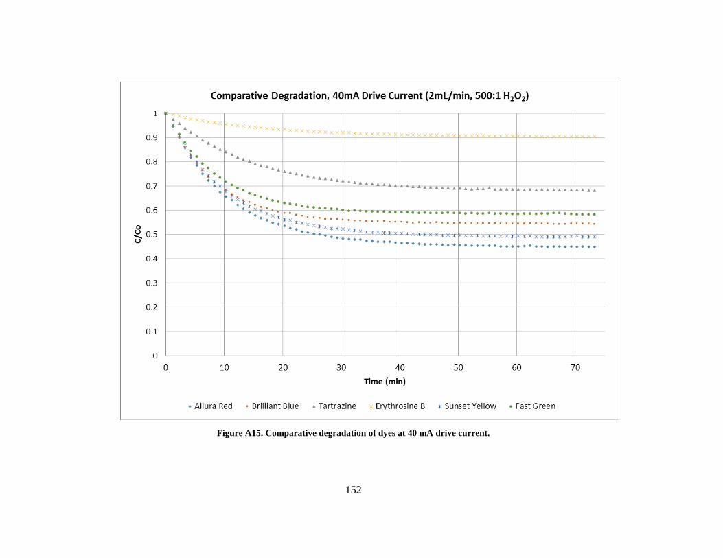
152


153


154


155


156


157

Figure A20. Bisphenol A degradation as a function of drive current.

158

Figure A21. 2,4-Dinitrotoluene degradation as a function of drive current.

159

Figure A22. Malathion degradation as a function of drive current.

160

Figure A23. Methyl tert-butyl ether degradation as a function of drive current.

161

Figure A24. Tert-butyl alcohol degradation as a function of drive current.

162

Figure A25. Comparative degradation of achromatic chemicals at 20 mA drive current.

163


164


165


166


167


168

Figure A31. Allura Red degradation as a function of peroxide ratio, 40 mA.

169

Figure A32. Allura Red degradation as a function of peroxide ratio, 200 mA.

170

Figure A33. Erythrosine B degradation as a function of peroxide ratio, 40 mA.

171


172


173


174

Figure A37. Fast Green degradation as a function of peroxide ratio, 200 mA.

175

Figure A38. Sunset Yellow degradation as a function of peroxide ratio, 120 mA.

176

Figure A39. Sunset Yellow degradation as a function of peroxide ratio, 200 mA.

177

Figure A40. Tartrazine degradation as a function of peroxide ratio, 120 mA.

178

Figure A41. Tartrazine degradation as a function of peroxide ratio, 200 mA.

179

Figure A42. Bisphenol A degradation as a function of peroxide ratio, 120 mA.

180

Figure A43. 2,4-DNT degradation as a function of peroxide ratio, 120 mA.

181

Figure A44. Malathion degradation as a function of peroxide ratio, 120 mA.

182

Figure A45. MTBE degradation as a function of peroxide ratio, 120 mA.

183

Figure A46. Comparative negative correlation between R2 of model fit and absorptivity values.

184

VII. Appendix B The table below and on subsequent pages contains an initial set of molecular descriptors generated from PubChem and Mold2for the dyes and achromatic chemicals utilized.

Descriptor Description

PC1 Molecular Weight

PC2 Molecular Formula

PC3 XLogP3

PC4 Hydrogen Bond Donor Count

PC5 Hydrogen Bond Acceptor Count

PC6 Rotatable Bond Count

PC7 Exact Mass

PC8 Monoisotopic Mass

PC9 Topological Polar Surface Area

PC10 Heavy Atom Count

PC11 Formal Charge

PC12 Complexity

PC13 Isotope Atom Count

PC14 Defined Atom Stereocenter Count

PC15 Undefined Atom Stereocenter Count

PC16 Defined Bond Stereocenter Count

PC17 Undefined Bond Stereocenter Count

PC18 Covalently-Bonded Unit Count

D001 number of 6-membered aromatic rings (only carbon atoms)

D002 Number of 03-membered rings





185






D012 number of multiple bonds

D013 number of circuits structure

D014 number of rotatable bonds

D015 rotatable bond fraction

D016 number of double bonds

D017 number of aromatic bonds

D018 sum of conventional bond orders (H-depleted)

D019 number of Hydrogen

D020 number of Helium

D021 number of Lithium

D022 number of Beryllium

D023 number of Boron

D024 number of Carbon

D025 number of Nitrogen

D026 number of Oxygen

D027 number of Fluorine

D028 number of Neon

D029 number of Sodium

D030 number of Magnesium

D031 number of Aluminum

D032 number of Silicon

D033 number of Phosphorus

D034 number of Sulfur

D035 number of Chlorine

186

D036 number of Argon

D037 number of Potassium

D038 number of Calcium

D039 number of Scandium

D040 number of Titanium

D041 number of Vanadium

D042 number of Chromium

D043 number of Manganese

D044 number of Iron

D045 number of Cobalt

D046 number of Nickel

D047 number of Copper

D048 number of Zinc

D049 number of Gallium

D050 number of Germanium

D051 number of Arsenic

D052 number of Selenium

D053 number of Bromine

D054 number of Krypton

D055 number of Rubidium

D056 number of Strontium

D057 number of Yttrium

D058 number of Zirconium

D059 number of Niobium

D060 number of Molybdenum

D061 number of Technetium

D062 number of Ruthenium

D063 number of Rhodium

D064 number of Palladium

187

D065 number of Silver

D066 number of Cadmium

D067 number of Indium

D068 number of Tin

D069 number of Antimony

D070 number of Tellurium

D071 number of Iodine

D072 number of Xenon

D073 number of Cesium

D074 number of Barium

D075 number of Lanthanum

D076 number of Cerium

D077 number of Praseodymium

D078 number of Neodymium

D079 number of Promethium

D080 number of Samarium

D081 number of Europium

D082 number of Gadolinium

D083 number of Terbium

D084 number of Dysprosium

D085 number of Holmium

D086 number of Erbium

D087 number of Thulium

D088 number of Ytterbium

D089 number of Lutetium

D090 number of Hafnium

D091 number of Tantalum

D092 number of Tungsten

D093 number of Rhenium

188

D094 number of Osmium

D095 number of Iridium

D096 number of Platinum

D097 number of Gold

D098 number of Mercury

D099 number of Thallium

D100 number of Lead

D101 number of Bismuth

D102 number of Polonium

D103 number of Astatine

D104 number of Radon

D105 number of Francium

D106 number of Radium

D107 number of Actinium

D108 number of Thorium

D109 number of Protactinium

D110 number of Uranium

D111 number of Neptunium

D112 number of Plutonium

D113 number of Americium

D114 number of Curium

D115 number of Berkelium

D116 number of californium

D117 number of Einsteinium

D118 number of Fermium

D119 number of Mendelevium

D120 number of Nobelium

D121 number of Lawrencium

D122 Molecular weight

189

D123 Average of molecular weight

D124 number of atoms in each molecule

D125 number of none-Hydrogen atoms in each molecule

D126 number of bonds in each molecule

D127 number of none-Hydrogen bonds in each molecule

D128 number of rings in each molecule

D129 number of triple bonds in each molecule

D130 number of halogen atoms in each molecule

D131 molecular size index

D132 atomic composition index

D133 mean value of atomic composition index

D134 Branch index

D135 Molecular structure connectivity index

D136 Narumi-type topological index

D137 Harmonic topological index

D138 Geometric topological index

D139 Topological distance count order-3

D140 log of vertex distance path count

D141 average of vertex distance path count

D142 Balaban type of mean square vertex distance index

D143 sum of atomic Van Der Waals Carbon-scale

D144 mean atomic van der Waals Carbon-scale

D145 sum of atomic electronegativities Pauling-Scale on Carbon

D146 mean atomic electronegativities Pauling-scaled on Carbon

D147 sum of atomic electronegativities Sanderson-scaled on Carbon

D148 mean atomic electronegativity Sanderson-scaled on Carbon

D149 sum of atomic electronegativity Allred-Rochow-scaled on Carbon

D150 mean atomic electronegativity Allred-Rochow-scaled on Carbon

D151 sum of atomic polarizabilities scaled on Carbon-SP3

190

D152 mean atomic polarizability scaled on Carbon-SP3

D153 Zagreb order-1 index

D154 Zagreb order-1 index with value of valence vertex degrees

D155 Zagreb order-2 index

D156 Vertex degree topological index

D157 second Zagreb order-2 index with value of valence vertex degrees

D158 valence electrons of principal quantum index

D159 Schultz type Molecular Topological index

D160 Schultz type Molecular Topological Index of valence vertex degrees

D161 Molecular Topological Distance Index

D162 Molecular Topological Distance Index of valence vertex degrees

D163 Molecular size and branching index

D164 index of terminal vertex matrix

D165 Wiener index

D166 Average Path length in Wiener Index

D167 reciprocal index of Wiener distance matrix

D168 Harary index

D169 Index of Laplacian Matrix

D170 First No-Zero eigenvalue of Laplacian matrix

D171 Wiener–Path index

D172 reciprocal Wiener-Path index

D173 Mohar order-2 index

D174 Maximum Path Index

D175 Wiener Type Maximum Path Index

D176 reciprocal Wiener Type Maximum Path Index

D177 Minimum-Path/Maximum-Path Index

D178 All-Path Wiener - sum of the edges in the shortest paths between all pairs of non-hydrogen atoms

D179 Heteroatoms and Multiple bonds weighted Distance Matrix

191

D180 Mass Weighted Distance Matrix

D181 Index of Van Der Waals Weighted Distance Matrix

D182 Distance Matrix of Electronegativity Weighted with Electronegativities Pauling-Scale

D183 Distance Matrix of Electronegativity Weighted with Sanderson Electronegativities

D184 Distance Matrix of Electronegativity Weighted with Allred-Rochow Electronegativites

D185 Polarizability weighted distance matrix

D186 Average vertex distance connectivity index

D187 Balaban heteroatoms bonds weighted index

D188 Balaban mass weighted index

D189 Balaban van der Waals weighted index

D190 Balaban electronegativity weighted with Pauling-Scale index

D191 Balaban electronegativity weighted with Sanderson-Scale index

D192 Balaban electronegativity weighted with Allred-Rochow-Scale index

D193 Balaban-type polarizability weighted index

D194 maximal valence vertex electrotopological negative variation

D195 maximal valence vertex electrotopological positive variation

D196 Sum absolute electrotopological negative variation

D197 Electrotopological index

D198 sum electrotopological states index

D199 mean electrotopological states index

D200 vertex connectivity order-0 index






D206 average vertex connectivity order-0 index



192




D212 valence vertex connectivity order-0 Index






D218 average valence vertex connectivity order-0 Index






D224 principal quantum vertex connectivity order-0 Index






D230 aromaticity valence vertex connectivity order-1 index

D231 sum of valence vertex connectivity order-1 index

D232 reciprocal distance order-1 sum product index

D233 squared reciprocal distance order-1 sum product index

D234 Kier atom's 0-order path information index

D235 Kier 1-path index



193

D238 Molecular flexibility index

D239 atom's connectivity index in longest path

D240 sum of the longest path of the atom

D241 average longest path of the molecule

D242 average of deviation of average of longest path

D243 average of deviation of distance degree

D244 shortest path in the molecule

D245 shortest path centralization index

D246 maximum value of variation

D247 EXP2 of Path-distance / Walk-distance over all atoms




D251 Petitjean index

D252 structure centric index

D253 structure lopping centric group index

D254 radial centric index

D255 vertex distance count equality index

D256 vertex distance count magnitude index

D257 total vertex distance count equality index

D258 total vertex distance count magnitude index

D259 mean of distance degree equality index

D260 mean of distance degree magnitude index

D261 information of vertex degree equality index

D262 information of bonds index

D263 vertex distance path count index

D264 complexity vertex distance path count index

D265 Vertex distance information index

D266 relative of vertex distance information index

194

D267 mean of vertex distance information index

D268 extended of vertex distance information index

D269 information content order-0 index






D275 total information content order-0 index






D281 structural information content order-0 index



D284 structural information content order3 index



D287 Complementary information content order-0 index



D290 Complementary information content order3 index



D293 bond information content order-0 index



195

D296 bond information content order3 index



D299 The largest eigenvalue

D300 spanning tree with log value

D301 Maximum eigenvalue weighted by Heteroatoms and Multiple bonds Matrix

D302 Maximum eigenvalue weighted by mass distance matrix

D303 Maximum eigenvalue weighted by van der Waals distance matrix

D304 Maximum eigenvalue weighted by polarizability distance matrix

D305 Maximum eigenvalue weighted by electronegativity Pauling-Scale distance matrix

D306 Maximum eigenvalue weighted by electronegativity Sanderson-Scale weighted distance matrix

D307 Maximum eigenvalue weighted by electronegativity Allred-Rochow-Scale distance matrix

D308 Sum eigenvalue weighted by Heteroatoms and Multiple bonds Distance Matrix

D309 Sum eigenvalue weighted by mass distance matrix

D310 Sum eigenvalue weighted by van der Waals distance matrix

D311 Sum eigenvalue weighted by polarizability distance matrix

D312 Sum eigenvalue weighted by electronegativity Pauling-Scale distance matrix

D313 Sum eigenvalue weighted by electronegativity Sanderson-Scale distance matrix

D314 Sum eigenvalue weighted by electronegativity Allred-Rochow-Scale distance matrix

D315 Sum absolute eigenvalue weighted by Heteroatoms and Multiple bonds Distance Matrix

D316 Sum absolute eigenvalue weighted by mass distance matrix

D317 Sum absolute eigenvalue weighted by van der Waals distance matrix

D318 Sum absolute eigenvalue weighted by polarizability distance matrix

D319 Sum absolute eigenvalue weighted by electronegativity Pauling-Scale distance matrix

D320 Sum absolute eigenvalue weighted by electronegativity Sanderson-Scale distance matrix

D321 Sum absolute eigenvalue weighted by electronegativity Allred-Rochow-Scale distance matrix

196

D322 distance+detour path with ring index of order 3










D332 distance+detour path on ring index of order 3 (circuits)










D342 molecular topological path index of order 02









197

D351 molecular topological multiple path index of order 03








D359 molecular topological all path index

D360 conventional bond index

D361 ratio of convention bonds with total path counts

D362 ratio of difference of conventional bonds and total path counts

D363 Randic index

D364 Balaban All-Path index

D365 Balaban Short-Path index

D366 sum of topological distance between the vertices N and N

D367 sum of topological distance between the vertices N and P

D368 sum of topological distance between the vertices N and O

D369 sum of topological distance between the vertices N and S

D370 sum of topological distance between the vertices N and F

D371 sum of topological distance between the vertices N and Cl

D372 sum of topological distance between the vertices N and Br

D373 sum of topological distance between the vertices N and I

D374 sum of topological distance between the vertices O and O

D375 sum of topological distance between the vertices O and S

D376 sum of topological distance between the vertices O and P

D377 sum of topological distance between the vertices O and F

D378 sum of topological distance between the vertices O and Cl

D379 sum of topological distance between the vertices O and Br

198

D380 sum of topological distance between the vertices O and I

D381 sum of topological distance between the vertices S and S

D382 sum of topological distance between the vertices S and P

D383 sum of topological distance between the vertices S and F

D384 sum of topological distance between the vertices S and Cl

D385 sum of topological distance between the vertices S and Br

D386 sum of topological distance between the vertices S and I

D387 sum of topological distance between the vertices P and P

D388 sum of topological distance between the vertices P and F

D389 sum of topological distance between the vertices P and Cl

D390 sum of topological distance between the vertices P and Br

D391 sum of topological distance between the vertices P and I

D392 sum of topological distance between the vertices F and F

D393 sum of topological distance between the vertices F and Cl

D394 sum of topological distance between the vertices F and Br

D395 sum of topological distance between the vertices F and I

D396 sum of topological distance between the vertices Cl and Cl

D397 sum of topological distance between the vertices Cl and Br

D398 sum of topological distance between the vertices Cl and I

D399 sum of topological distance between the vertices Br and Br

D400 sum of topological distance between the vertices Br and I

D401 sum of topological distance between the vertices I and I

D402 walk count order-01






D408 walk count max-10 steps

199

D409 walk-returning count order-1






D415 topological structure autocorrelation length-1 weighted by atomic masses








D423 topological structure autocorrelation length-1 weighted by atomic van der Waals volumes








D431 topological structure autocorrelation length-1 weighted by atomic Sanderson electronegativities

200








D439 topological structure autocorrelation length-1 weighted by atomic polarizabilities








D447 Geary topological structure autocorrelation length-1 weighted by atomic masses








D455 Geary topological structure autocorrelation length-1 weighted by atomic van der Waals volumes

201








D463 Geary topological structure autocorrelation length-1 weighted by atomic Sanderson electronegativities








D471 Geary topological structure autocorrelation length-1 weighted by atomic polarizabilities



202






D479 Moran topological structure autocorrelation length-1 weighted by atomic masses








D487 Moran topological structure autocorrelation length-1 weighted by atomic van der Waals volumes








203

D495 Moran topological structure autocorrelation length-1 weighted by atomic Sanderson electronegativities








D503 Moran topological structure autocorrelation length-1 weighted by atomic polarizabilities








D511 Molecular topological order-1 charge index



204








D521 Mean molecular topological order-1 charge index










D531 Sum of molecular topological mean charge index

D532 Lowest eigenvalue from Burden matrix weighted by masses order-1








D540 Lowest eigenvalue from Burden matrix weighted by van der Walls order-1



205






D548 Lowest eigenvalue from Burden matrix weighted by electronegativities Sanderson-Scale order-1








D556 Lowest eigenvalue from Burden matrix weighted by polarizabilities order-1








D564 Highest eigenvalue from Burden matrix weighted by masses order-1



206






D572 Highest eigenvalue from Burden matrix weighted by van der Walls order-1








D580 Highest eigenvalue from Burden matrix weighted by electronegativities Sanderson-Scale order-1








D588 Highest eigenvalue from Burden matrix weighted by polarizabilities order-1



207






D596 number of total primary C-sp3

D597 number of total secondary C-sp3

D598 number of total tertiary C-sp3

D599 number of total quaternary C-sp3

D600 number of ring secondary C-sp3

D601 number of ring tertiary C-sp3

D602 number of ring quaternary C-sp3

D603 number of unsubstituted aromatic C-sp2

D604 number of substituted aromatic C-sp2

D605 number of primary C-sp2

D606 number of secondary C-sp2

D607 number of tertiary C-sp2

D608 number of group allenes

D609 number of terminal C-sp

D610 number of non-terminal C-sp

D611 number of group cyanates (aliphatic)

D612 number of group cyanates (aromatic)

D613 number of group isocyanates (aliphatic)

D614 number of group isocyanates (aromatic)

D615 number of group thiocyanates (aliphatic)

D616 number of group thiocyanates (aromatic)

D617 number of group isothiocyanates (aliphatic)

D618 number of group isothiocyanates (aromatic)

D619 number of group carboxylic acids (aliphatic)

208

D620 number of group carboxylic acids (aromatic)

D621 number of group esters (aliphatic)

D622 number of group esters (aromatic)

D623 number of group primary amides (aliphatic)

D624 number of group primary amides (aromatic)

D625 number of group secondary amides (aliphatic)

D626 number of group secondary amides (aromatic)

D627 number of group tertiary amides (aliphatic)

D628 number of group tertiary amides (aromatic)

D629 number of group carbamates (aliphatic)

D630 number of group carbamates (aromatic)

D631 number of group acyl halogenides (aliphatic)

D632 number of group acyl halogenides (aromatic)

D633 number of group thioacids (aliphatic)

D634 number of group thioacids (aromatic)

D635 number of group ditioacids (aliphatic)

D636 number of group ditioacids (aromatic)

D637 number of group thioesters (aliphatic)

D638 number of group thioesters (aromatic)

D639 number of group dithioesters (aliphatic)

D640 number of group dithioesters (aromatic)

D641 number of group aldehydes (aliphatic)

D642 number of group aldehydes (aromatic)

D643 number of group ketones (aliphatic)

D644 number of group ketones (aromatic)

D645 number of group urea derivatives

D646 number of group urea derivatives (aromatic)

D647 number of group primary amines (aliphatic)

D648 number of group primary amines (aromatic)

209

D649 number of group secondary amines (aliphatic)

D650 number of group secondary amines (aromatic)

D651 number of group tertiary amines (aliphatic)

D652 number of group tertiary amines (aromatic)

D653 number of group N-hydrazines (aliphatic)

D654 number of group N-hydrazines (aromatic)

D655 number of group N-azo (aliphatic)

D656 number of group N-azo (aromatic)

D657 number of group nitriles (aliphatic)

D658 number of group nitriles (aromatic)

D659 number of group imines (aliphatic)

D660 number of group imines (aromatic)

D661 number of group ammonia groups (aliphatic)

D662 number of group ammonia groups (aromatic)

D663 number of group hydroxylamines (aliphatic)

D664 number of group hydroxylamines (aromatic)

D665 number of group oximes (aliphatic)

D666 number of group oximes (aromatic)

D667 number of group N-nitroso (aliphatic)

D668 number of group N-nitroso (aromatic)

D669 number of group nitroso (aliphatic)

D670 number of group nitroso (aromatic)

D671 number of group nitro (aliphatic)

D672 number of group nitro (aromatic)

D673 number of group imides

D674 number of group total hydroxyl groups

D675 number of group phenols

D676 number of group primary alcohols (aliphatic)

D677 number of group secondary alcohols (aliphatic)

210

D678 number of group tertiary alcohols (aliphatic)

D679 number of group ethers (aliphatic)

D680 number of group ethers (aromatic)

D681 number of group hypohalogenydes (aliphatic)

D682 number of group hypohalogenydes (aromatic)

D683 number of group water molecules

D684 number of group sulfoxides

D685 number of group sulfones

D686 number of group sulfates

D687 number of group thioles

D688 number of group thioketones

D689 number of group sulfides

D690 number of group disulfides

D691 number of group sulfonic acids

D692 number of group sulfonamides

D693 number of group phosphites

D694 number of group phosphates

D695 number of group phosphothionates

D696 number of group phosphodithionates

D697 number of group phosphothioates

D698 number of group CH2X

D699 number of group CR2HX

D700 number of group CR3X

D701 number of group R=CHX

D702 number of group R=CRX

D703 number of group R#CX

D704 number of group CHRX2

D705 number of group CR2X2

D706 number of group R=CX2

211

D707 number of group RCX3

D708 number of group X-C on aromatic ring

D709 number of group X-C- on ring

D710 number of group X-C= on ring

D711 number of group X-C on conjugated C

D712 number of group donor atoms for H-bonds (with N and O)

D713 number of group acceptor atoms for H-bonds (N O F)

D714 number of group CH3R and CH4

D715 number of group CH2R2

D716 number of group CHR3

D717 number of group CR4

D718 number of group CH3X

D719 number of group CH2RX

D720 number of group CH2X2

D721 number of group CHR2X

D722 number of group CHRX2

D723 number of group CHX3

D724 number of group CR3X

D725 number of group CR2X2

D726 number of group CRX3

D727 number of group CX4

D728 number of group =CH2

D729 number of group =CHR

D730 number of group =CR2

D731 number of group =CHX

D732 number of group =CRX

D733 number of group =CX2

D734 number of group #CH

D735 number of group #CR or R=C=R

212

D736 number of group #CX

D737 number of group R~CH~R

D738 number of group R~CR~R

D739 number of group R~CX~R

D740 number of group Al-CH=X

D741 number of group Ar-CH=X

D742 number of group Al-C(=X)-Al

D743 number of group Ar-C(=X)-R

D744 number of group R-C(=X)-X / R-C#X

D745 number of group X-C(=X)-X

D746 number of group H attached to C0(sp3) no X attached to next C

D747 number of group H attached to heteroatom

D748 number of group H attached to C0(sp3) with 1X attached to next C




D752 number of group alcohol

D753 number of group phenol or enol or carboxyl OH

D754 number of group O=

D755 number of group Al-O-Al

D756 number of group Al-O-Ar or Ar-O-Ar or R-O-C=X

D757 number of group Al-NH2

D758 number of group Al2-NH

D759 number of group Al3-N

D760 number of group Ar-NH2 or X-NH2

D761 number of group Ar-NH-Al

D762 number of group Ar-NAl2

D763 number of group RCO-N< or >N-X=X

D764 number of group Ar2NH or Ar3N or Ar2N-Al

213

D765 number of group R#N or R=N

D766 r of group Ar-NO2 or RO-NO2

D767 number of group Al-NO2

D768 number of group Ar-N=X or X-N=X

D769 number of group R-SH

D770 number of group R2S or RS-SR

D771 number of group R=S

D772 number of group R-SO-R

D773 number of group R-SO2-R

D774 unsaturation index weighted by conventional bonds order

D775 hydrophilic factor index

D776 aromatic bonds ratio

D777 Molecular regression coefficients surface LogP index

214

Bibliography Air Force Civil Engineer Center. 2017. "US Air Force Civil Engineer Center." Air Force

PFOS/PFOA Snapshot. June 22. Accessed June 29, 2017. http://www.afcec.af.mil/WhatWeDo/Environment/Perfluorinated-Compounds/.

Anderson, Richard H, Janet K Anderson, and Paul A Bower. 2012. "Co-concurrence of 1,4-dioxane with Trichloroethylene in Chlorinated Solvent Groundwater Plumes at US Air Force Installations: Fact or Fiction." Integrated Environmental Assessment and Management 731-737.

Andreozzi, R, V Caprio, A Insola, and R Marotta. 1999. "Advanced Oxidation Process (AOP) for Water Purification and Recovery." Catalysis Today 51-59.

Apostol, Laura C, Camelia Smaranda, Mariana Diaconu, and Maria Gavrilescu. 2015. "Preliminary Ecotoxicological Evaluation of Erythrosin B and Its Photocatalytic Degradation Products." Environmental Engineering and Management Journal 465-471.

Atlantium Technologies. 2017. Medium Pressure and Low Pressure Lamps. Accessed May 17, 2017. http://www.atlantium.com/en/markets/aquaculture-eng/blog/medium-pressure-low-pressure-lamps.html.

Badawy, M, M Ghaly, and T Gad-Allah. 2006. "Advanced oxidation processes for the removal of organophosphorus pesticides from wastewater." Desalination 166-175.

Bairagi, Rinku, and Rakshit Ameta. 2016. "Photocatalytic Degradation of Erythrosine by Using Manganese Doped TiO2 Supported on Zeolite." International Journal of Chemical Sciences 1768-1776.

Barry, Judith A. 2012. Characterization of DoD Installation Wastewater Treatment. Technical, Noblis Center for Sustainability.

Beltran, Fernando J, Jose M Encinar, and Miguel A Alonso. 1998. "Nitroaromatic Hydrocarbon Ozonation in Water: Combined Ozonation with Hydrogen Peroxide or UV Radiation." Industrial and Engineering Chemical Research 32-40.

Benjamin, Mark M, and Desond F Lawler. 2013. Water Quality Engineering. Hoboken: Wiley.

215

Bohrerova, Z, G Bohrer, S Mohanraj, J Ducoste, and K Linden. 2005. "Experimental measurements of fluence distribution in a UV reactor using fluorescent microspheres." Environmental Science and Technology 8925-8930.

Borhani, Tohid, Mohammadhossein Saniedanesh, Mehdi Bagheri, and Jeng S. Lim. 2016. "QSPR Prediction of the Hydroxyl Radical Rate Constant of Water Contaminants." Water Research 344-353.

Buxton, G, C Greenstock, W Helman, and A Ross. 1988. "Critical review of rate constants for reactions of hydrated electrons, hydrogen atoms, and hydroxyl radicals in aqueous solution." Journal of Physical and Chemical Reference Data 513-531.

Chang, M, C Chung, J Chern, and T Chen. 2010. "Dye decomposition kinetics by UV/H2O2: initial rate analysis by effective kinetic modeling methodology." Chemical Engineering Science 135-140.

Chen, Jingwen, Degao Wang, Shuanglin Wang, Xianliang Qiao, and Liping Huang. 2007. "Quantitative structure–property relationships for direct photolysis of polybrominated diphenyl ethers." Ecotoxicology and Environmental Safety 348-352.

Crittenden, J, S Hu, D Hand, and S Green. 1999. "A kinetic model for H2O2/UV process in a completely mixed batch reactor." Water Research 2315-2328.

Dorfman, Leon M, and Gerald E Adams. 1973. Reactivity of the Hydroxyl Radical in Aqueous Solutions. Technical Report, Washington: National Bureau of Standards.

Duckworth, Kelsey, Michael Spencer, Christopher Bates, Michael E. Miller, Catherine Almquist, Michael Grimaila, Matthew Magnuson, Stuart Willison, Rebecca Phillips, and LeeAnn Racz. 2015. "Advanced oxidation degradation kinetics as a function of ultraviolet LED duty cycle." Water Science and Technology 1375-1381.

Edalatmanesh, M, R Dhib, and M Mehrvar. 2008. "Kinetic modeling of aqueous phenol degradation by UV/H2O2 process." International Journal of Chemical Kinetics 34-43.

Englehardt, James D, Tingting Wu, Frederick Bloetscher, Yang Deng, Piet du Pisani, Sebastian Eilert, Samir Elmir, et al. 2016. "Net-Zero Water Management: Achieving Energy-Positive Municipal Water Supply." Environmental Science: Water Research and Technology 250-260.

216

Famiglietti, Jay. 2014. "Epic California Drought and Groundwater: Where Do We Go from Here?" Water Currents.

Ferguson, Grant, and Tom Gleeson. 2013. "Threats to Coastal Aquifers." Nature Climate Change 605-606.

Fukui, Kenichi. 1981. "The role of frontier orbitals in chemical reactions - Nobel lecture." Chemistry 9-26.

Gallucci, D. 2016. Material and Design Considerations for a Portable Ultraviolet (UV) Light Emitting Diode (LED) Water Purification Device. Masters Thesis, Wright-Patterson AFB: Air Force Institute of Technology.

Ghafoorim, S, M Mehrvar, and P Chan. 2014. "Photoreactor scale-up for degradation of aqueous poly(vinyl alcohol) using UV/H2O2 process." Chemical Engineering Journal 133-142.

Gillis, Regina. 2006. US Air Force. March 28. Accessed April 28, 2017. http://www.af.mil/News/Article-Display/Article/131533/california-base-wins-water-recycling-award/.

Giri, R, H Ozaki, Y Takayanagi, S Taniguchi, and R Takanami. 2011. "Efficacy of ultraviolet radiation and hydrogen peroxide oxidation to eliminate large number of pharmaceutical compounds in mixed solution." International Journal of Environmental Science and Technology 19-30.

Gligorovski, S, R Strekowski, S Barbati, and D Vione. 2015. "Environmental implications of hydroxyl radicals." Chemical Reviews 13051-13092.

Grcic, I, S Papic, D Mesec, N Koprivanac, and D Vujevic. 2014. "The kinetics and efficiency of UV assisted advanced oxidation of various types of commercial organic dyes." Journal of Photochemistry and Photobiology A: Chemistry 49-58.

Hartog, N, M Mahmoodlu, and S Hassanizadeh. 2015. "Bias by inappropriate use of the pseudo-first order approach to estimate second-order reaction rate constants: reply to the commentary by Tratnyek." Science of the Total Environment 724-725.

Hong, H, Q Xie, W Ge, F Qian, F Fang, L Shi, Z Su, R Perkins, and W and Tong. 2008. "Mold2, molecular descriptors from 2D structures for chemoinformatics and toxicoinformatics." Journal of Chemical Information and Modeling 1337-1344.

217

Hong, Huixiao, Svetoslav Slavov, Weigong Ge, Feng Qian, Zhenqiang Su, Hong Fang, Yiyu Cheng, Roger Perkins, Leming Shi, and Weida Tong. 2012. "Mold2 Molecular Descriptors for QSAR." In Statistical Modelling of Molecular Descriptors in QSAR/QSPR, by Matthias Dehmer, Kurt Varmuza and Danail Bonchev, 65-110. Weinheim: Wiley-Blackwell.

Huang, Xiangfeng, Yi Feng, Cui Hu, Xiaoyu Xiao, Daliang Yu, and Xiaoming Zou. 2015. "Mechanistic QSAR models for Interpreting Degradation Rates of Sulfonamides in UV-Photocatalysis Systems." Chemosphere 183-189.

Huber, Marc M, Silvio Canonica, Gun-Young Park, and Urs Von Gunten. 2003. "Oxidation of Pharamceuticals During Ozonation and Advanced Oxidation Processes." Environmental Science and Technology 1016-1024.

Ibrahim, MA, J MacAdam, O Autin, and B Jefferson. 2014. "Evaluating the Impact of LED Bulb Development on the Economic Viability of Ultraviolet Technology for Disinfection." Environmental Technology 400-406.

Jenny, R, O Simmons, M Shatalov, and J Ducoste. 2014. "Modeling a continuous flow ultraviolet Light Emitting Diode reactor using computational fluid dynamics." Chemical Engineering Science 524-535.

Jin, Xiaohui, Sigrid Peldszus, and Peter M Huck. 2015. "Predicting the Reaction Rate Constants of Micropollutants with Hydroxyl Radicals in Water Using QSPR Modeling." Chemosphere 1-9.

Katsoyiannis, Ioannis A, Silvio Canonica, and Urs von Gunten. 2011. "Efficiency and Energy Requirements for the Transformation of Organic Micropollutants by Ozone, O3/H2O2, and UV/H2O2." Water Research 3811-3822.

Kim, I, N Yamashita, and H Tanaka. 2009. "Photodegradation of pharmaceuticals and personal care products during UV and UV/H2O2 treatments." Chemosphere 518-525.

Kusic, Hrvoje, Bakhtiyor Rasulev, Danuta Leszczynska, Jerzy Leszczynski, and Natalija Koprivanac. 2009. "Prediction of rate constants for radical degradation of aromatic pollutants in water matrix: A QSAR study." Chemosphere 1128-1134.

Lee, Yunho, and Urs von Gunten. 2012. "Quantitative structure–activity relationships (QSARs) for the transformation of organic micropollutants during oxidative water treatment." Water Research 6177-6195.

218

Luo, Y.R. 2007. Comprehensive Handbook of Chemical Bond Energies. Boca Raton: CRC Press.

Mandavgane, S, and M Yenkie. 2011. "Degradation of salicylic acid by UV, UV/H2O2, UV/O3, photo-Fenton processes." Journal of Chemistry 640-647.

Marcum, C. 2014. Measurements of DNA Damage and Repair in Bacillus Anthracis Sterne Spores by UV Radiation. Masters Thesis, Wright-Patterson AFB: Air Force Institute of Technology.

Mariani, M, R Brandi, A Cassano, and C Zalazar. 2013. "A kinetic model for the degradation of dichloroacetic acid and formic acid in water employing the H2O2/UV process." Chemical Engineering Journal 423-432.

Meylan, William M., and Philip H Howard. 2003. "A review of quantitative structure-activity relationship methods for the prediction of atmospheric oxidation of organic chemicals." Environmental Toxicology and Chemistry 1724-1732.

Minakata, D, S Mezyk, J Jones, B Daws, and J Crittenden. 2014. "Development of Linear Free Energy Relationships for Aqueous Phase Radical-Involved Chemical Reactions." Environmental Science and Technology 13925-13932.

Minakata, Daisuke, Ke Li, Paul Westerhoff, and John Crittenden. 2009. "Development of a Group Contribution Method to Predict Aqueous Phase Hydroxyl Radical Reaction Rate Constants." Environmental Science and Technology 6220-6227.

Morckel, Victoria. 2017. "Why the Flint, Michigan, USA Water Crisis is an Urban Planning Failure." Cities 23-27.

Mudimbi, P. 2015. Pulsed Ultraviolet Light Emitting Diodes for Advanced Oxidation of Tartrazine. Masters Thesis, Wright-Patterson AFB: Air Force Institute of Technology.

Murcia, M, N Vershinin, N Briantceva, M Gomez, E Gomez, E Cascales, and A Hidalgo. 2015. "Development of a kinetic model for the UV/H2O2photodegradationof 2,4-dichlorophenoxiacetic acid." Chemical Engineering Journal 356-367.

Muruganandham, M, and M Swaminathan. 2004. "Photochemical oxidation of reactive azo dye with UV-H2O2 process." Dyes and Pigments 269-275.

219

Narayansamy, L, and T Murugesan. 2014. "Degradation of Alizarin Yellow R using UV/H2O2 advanced oxidation process." Environmental Progress and Sustainable Energy 482-489.

National Institutes of Health. 2016. "National Center for Biotechnology Information." PubChem. January 17. Accessed January 17, 2016. https://pubchem.ncbi.nlm.nih.gov/#.

Oancea, P, and V Meltzer. 2013. "Kinetics of tartrazine photodegradation by UV/H2O2 in aqueous solution." Chemical Papers 105-111.

O'Boyle, Noel M, Michael Banck, Craig A James, Chris Morley, Tim Vandermeersch, and Geoffrey R Hutchinson. 2011. "Open Babel: An Open Chemical Toolbox." Journal of Chemoinformatics.

Ohura, Takeshi, Takashi Amagai, and Masakazu Makino. 2008. "Behavior and prediction of photochemical degradation of chlorinated polycyclic aromatic hydrocarbons in cyclohexane." Chemosphere 2110-2117.

Oppenlander, T. 2003. Photochemical Purification of Water and Air - Advanced Oxidation Processes (AOPs): Principles, Reaction Mechanisms, Reactor Concepts. Darmstadt, Germany: Wiley-Vch.

Pro-Act. 2000. Spotlight On: Luke Air Force Base. Success Story, San Antonio: Air Force Center for Environmental Excellence.

Rahmani, Z, M Kermani, M Gholami, A Jafari, and N Mahmoodi. 2012. "Effectiveness of photochemical and sonochemical processes in degradation of Basic Violet 16 (BV16) dye from aqueous solutions." Iranian Journal of Environmental Health Science and Engineering 1-7.

Rajagopalan, Balaji, Kenneth Nowak, James Prairie, Martin Hoerling, Benjamin Harding, Joseph Barsugli, Andrea Ray, and Bradley Udall. 2009. "Water Supply Risk on the Colorado River: Can Management Mitigate?" Water Resources Research 1-7.

Rodriguez, Clemencia, Paul Van Buynder, Richard Lugg, Palenque Blair, Brian Devine, Angus Cook, and Philip Weinstein. 2009. "Indirect Potable Reuse: A Sustainable Water Alternative." International Journal of Environmental Research and Public Health 1174-1203.

Rosario-Ortiz, F, E Wert, and S Snyder. 2010. "Evaluation of UV/H2O2 treatment for the oxidation of pharmaceuticals in wastewater." Water Research 1440-1448.

220

Salinas, Alex. 2013. Air Force directive prompts water conservation. July 11. Accessed May 7, 2017. http://www.jbsa.mil/News/News/Article/461563/air-force-directive-prompts-water-conservation/.

Sanches, S, Crespo MT Barreto, and VJ Pereira. 2010. "Drinking Water Treatment of Priority Pesticides Using Low Pressure UV Photolysis and Advanced Oxidation Processes." Water Research 1809-1818.

Santoro, D, M Raisee, M Moghaddami, J Ducoste, M Sasges, L Liberti, and M Notarnicola. 2010. "Modeling hydroxyl radical distribution and trialkyl phosphates oxidation in UV - H2O2 photoreactors using computational fluid dynamics." Environmental Science and Technology 6233-6241.

Scott, R, P Mudimbi, M.E. Miller, M Magnuson, S Willison, R Phillips, and Willie F Harper Jr. 2016. "dvanced oxidation of tartrazine and Brilliant Blue with pulsed ultraviolet light emitting diodes." Water Environment Research Vol 88.

Scott, Robert W. 2015. The Use of Ultra-violet (UV) Light Emitting Diodes (LEDs) in an Advanced Oxidation Process (AOP) with Brilliant Blue FCF as an Indicator. Masters Thesis, Wright-Patterson AFB: Air Force Institute of Technology.

Sharma, S. 2015. Green Chemistry for Dyes Removal from Waste Water. Hoboken: Wiley.

Shu, Z, J Bolton, M Belosevic, and M Gamal El Din. 2013. "Photodegradation of emerging micropollutants using the medium-pressure UV/H2O2 Advanced Oxidation Process." Water Research 2881-2889.

Singh, K, S Gupta, N Basant, and D Mohan. 2014. "QSTR Modeling for qualitative and quantitative toxicity predictions of diverse chemical pesticides in honey bee for regulatory purposes." Chemical Research in Toxicology 1504-1515.

Stefan, Mihaela I, john Mack, and James R Bolton. 2000. "Degradation Pathways during the Treatment of Methyl tert-Butyl Ether by the UV/H2O2 Process." Environmental Science and Technology 650-658.

Stewart, B. 2016. Pulsed Ultraviolet Light Emitting Diodes for Advanced Oxidation of Tartrazine and Disinfection of Deployed Asset Drinking Water. Masters Thesis, Wright-Patterson AFB: Air Force Institute of Technology.

Stuart Computational Chemistry. 2016. MOPAC. Accessed July 21, 2016. http://openmopac.net/index.html.

221

Sudhakaran, Sairam, and Gary Amy. 2013. "QSAR models for oxidation of organic micropollutants in water based on ozone and hydroxyl radical rate constants and their chemical classification." Water Research 1111-1122.

Sudhakaran, Sairam, James Calvin, and Gary L. Amy. 2012. "QSAR models for the removal of organic micropollutants in four different river water matrices." Chemosphere 144-150.

Sullivan, Abigail, Dave D White, Kelli L Larson, and Amber Wutich. 2017. "Towards Water Sensitive Cities in the Colorado River Basin: A Comparative Historical Analysis to Inform Future Water Sustainability Transitions." Sustainability 1-27.

Tang, Water Z. 2004. Physicochemical Treatment of Hazardous Wastes. Boca Raton: Lewis Publishers.

US Air Force. 2013. US Air Force Energy Strategic Plan. Washington: SAF/IE.

US Army. 2015. Army Techniques Publication 4-44, Water Support Operations. Washington: Headquarters Dept of the Army.

US Department of Energy. 2015. "US Department of Energy." Federal Energy and Water Management Awards 2014. January. Accessed May 3, 2017. https://energy.gov/sites/prod/files/2015/01/f19/fewma2014_usaf_hurlburt_field.pdf.

US Food and Drug Administration. 2015. "US Food and Drug Administration." Bioinformatics Tools: Mold2. September 30. Accessed December 7, 2015. https://www.fda.gov/ScienceResearch/BioinformaticsTools/Mold2/default.htm.

USEPA. 1999. Alternative Disinfectants and Oxidants Guidance Manual. Washington: Office of Water.

—. 2016. Net Zero Concepts and Definitions. September 16. Accessed February 18, 2017. https://19january2017snapshot.epa.gov/water-research/net-zero-concepts-and-definitions_.html.

Vilhunen, S, and M Sillanpaa. 2009. "Ultraviolet light emitting diodes and hydrogen peroxide in the photodegradation of aqueous phenol." Journal of Hazardous Materials 1530-1534.

222

Wang, Ya-nan, Jingwen Chen, Xuehua Li, Siyu Zhang, and Xianlianng Qiao. 2009. "Estimation of Aqueous-Phase Reaction Rate Constants of Hydroxyl Radical with Phenols, Alkanes and Alcohols." QSAR and Combinatorial Science 1309-1316.

Wavefunction. 2017. "Wavefunction Inc." Spartan Software. Accessed May 12, 2017. https://www.wavefun.com/products/spartan.html.

Wols, B, and C Hofman-Caris. 2012. "Review of photochemical reaction constants of organic micropollutants required for UV advanced oxidation in water." Water Research 2815-2827.

Yee, Liew C, and Yap C Wei. 2012. "Current Modeling Methods Used in QSAR/QSPR." In Statistical Modelling of Molecular Descriptors in QSAR/QSPR, by Matthias Dehmer, Kurt Varmuza and Danail Bonchev, 1-31. Weinheim: Wiley-Blackwell.

223

Vita

Lieutenant Colonel John E. Stubbs was born and raised in North Carolina. After

graduating from Saint Stephens High School in Hickory, NC in 1993, he attended North

Carolina State University. He graduated Summa Cum Laude in 1998 with a bachelor’s

degree in Industrial Engineering.

In 1998, he started a brief career with Procter and Gamble where he worked as a

process engineer dedicated to raw material supply chain management and quality control

for antiperspirant and deodorant manufacturing. In 2001, an altruistic calling drove a

desire for Lieutenant Colonel Stubbs to serve his country in the United States Air Force.

He was selected for direct commissioning and entered the Bioenvironmental Engineering

career field in January 2002.

After initial training, Lieutenant Colonel Stubbs was assigned to his first

operational assignment with the Air Force Research Laboratory at Wright-Patterson

AFB, Ohio as a principal investigator in the Human Effectiveness Directorate,

Biodynamics and Acceleration Branch. There he was responsible for research programs

related to aircrew seat system comfort, safety, and standardization and garnered $1.2

million in research funding. He also served as the alternate Unit Environmental

Coordinator for the Human Effectiveness Directorate, responsible for cradle-to-grave

compliance with hazardous material and hazardous waste management.

In 2005, he was assigned to the 62nd Airlift Wing at McChord AFB, Washington

where he was assigned to the 62nd Medical Operations Squadron, Bioenvironmental

Engineering Element and was responsible for environmental, radiation safety, and

224

CBRNE response programs. During this time, he was deployed to Camp Lemonier,

Djibouti in 2007 in support of the US Army’s 350th CACOM Functional Specialty Team

conducting medical and veterinary civil affairs programs in countries across the Horn of

Africa.

In 2008, Lieutenant Colonel Stubbs was accepted to pursue a Master’s Degree

program at the Air Force Institute of Technology (AFIT) and returned to Wright

Patterson AFB. There, he began a Master of Science in Industrial Hygiene, specializing

in design of a novel noise delivery system for jet fuel aerosol ototoxicity studies.

Upon graduation from AFIT in 2010 he was assigned as chief of

Bioenvironmental Engineering Education and Training Branch at the USAF School of

Aerospace Medicine (USAFSAM) where he was responsible for all facets of curriculum

development and maintenance for officer and enlisted courses. Additionally, he

completed the USAF Basic Instructor Course and completed all required instructor

internship hours to receive full instructor certification. While at USAFSAM, he was also

assigned to the Air Force Radiation Assessment Team as Surveillance Team Chief and

deployed to Japan in 2011 in support of Operation TOMODACHI, following the tsunami

and subsequent nuclear reactor emergency.

In 2011, Lieutenant Colonel Stubbs moved to the 509th Bomb Wing at Whiteman

AFB, Missouri. There he was assigned to the 509th Medical Operations Squadron as

Bioenvironmental Engineering Flight Commander. He was responsible for all facets of

bioenvironmental engineering programs in support of 3,000 personnel and four airframes.

During this time, he was also deployed to Bagram Air Base, Afghanistan as

225

Bioenvironmental Engineering Element Chief, supporting a population of 30,000

personnel with all bioenvironmental engineering core competencies.

He returned to Wright Patterson AFB, Ohio in 2014 to begin his doctorate degree

at AFIT. Upon graduation, he will be assigned to AFIT faculty in the Graduate School of

Engineering and Management.

14-09-2017 Doctoral Dissertation August 2014 - September 2017

Dynamics of Chemical Degradation in Water Using Photocatalytic Reactionsin an Ultraviolet Light Emitting Diode Reactor

Stubbs, John E., Lieutenant Colonel, USAF

Air Force Institute of TechnologyGraduate School of Engineering and Management (AFIT/EN)2950 Hobson WayWright-Patterson AFB OH 45433-7765


Intentionally Left Blank

Distribution Statement A: Approved for Public Release; Distribution Unlimited.

This work is declared a work of the U.S. Government and is not subject to copyright protection in the United States.

This work examined ultraviolet (UV) light emitting diodes (LED) and hydrogen peroxide in an advanced oxidation process insupport of a USAF installation net zero water initiative. A UV LED reactor was used for degradation of soluble organic chemicals.There were linear relationships between input drive current, optical output power, and first order degradation rate constants. Whendrive current was varied, first order degradation rates depended on chemical identities and the drive current. When molar peroxideratios were varied, kinetic profiles revealed peroxide-limited or radical-scavenged phenomena. Molar absorptivity helped explainthe complexity of chemical removal profiles. Degradation kinetics were used to compare fit of molecular descriptors from publishedquantitative structure property relationship (QSPR) models. A novel QSPR model was built using zero point energy and molarabsorptivity as predictors. Finally, a systems architecture was used to describe a net zero water program and proposed areas for UVLED reactor integration. Facility-level wastewater treatment was found to be the most feasible near-term application.

Ultraviolet, light emitting diodes, advanced oxidation process, chemical degradation, net zero water, systems architecture

U U U UU 239

Dr. Willie F. Harper, Jr., AFIT/ENV

(937) 255-3636 x4528 [email protected]

dynamics of chemical degradation in water using ...dynamics of chemical degradation in water using...

Documents