dynamics of a prey-predator system with infection in … · dynamics of a prey-predator system with...

Electronic Journal of Differential Equations, Vol. 2017 (2017), No. 209, pp. 1–27.

ISSN: 1072-6691. URL: http://ejde.math.txstate.edu or http://ejde.math.unt.edu

DYNAMICS OF A PREY-PREDATOR SYSTEM WITHINFECTION IN PREY

SHASHI KANT, VIVEK KUMAR

Communicated by Zhaosheng Feng

Abstract. This article concerns a prey-predator model with linear functional

response. The mathematical model has a system of three nonlinear coupledordinary differential equations to describe the interaction among the healthy

prey, infected prey and predator populations. Model is analyzed in terms ofstability. By considering the delay as a bifurcation parameter, the stability of

the interior equilibrium point and occurrence of Hopf-bifurcation is studied.

By using normal form method, Riesz representation theorem and center mani-fold theorem, direction of Hopf bifurcation and stability of bifurcated periodic

solutions are also obtained. As the real parameters are not available (because

it is not a case study). To validate the theoretical formulation, a numericalexample is also considered and few simulations are also given.

1. Introduction

The study of prey-predator systems has been a burning topic of research for sev-eral years. The pioneer work of Kermack and Mckendrick on Susceptible-Infective-Recovered-Susceptible (SIRS) models [9] have been widely accepted among re-searchers and scientific community. After the work of Kermack and Mckendrick[9] many mathematical models have been published ([3, 6, 16, 18, 21] etc. andreferences therein). M. Haque et al [3] proposed and analyzed a predator preymodel using standard disease incidence. They observed that the disease in theprey may avoid extinction of predators and its presence can destabilize an oth-erwise stable configuration of species. In [16], Naji and Mustafa investigated thedynamical nature of an eco-epidemiological model by applying nonlinear diseaseincidence rate among living species of the ecosystem. They proposed and investi-gated with regards to local and global dynamical nature of Holling type-II modelwith Susceptible-Infective type of disease in prey [16]. Jang and Baglama [18] pro-posed a deterministic continues time ecological model with the effect of parasites,where it is assumed that intermediate host for the parasites are the prey speciesand observed the dynamics of it. They conclude that parasites are in position toaffect the dynamics of the predator prey interaction due to infection. Jang andBaglama [18] have also proposed a stochastic version of the model and simulated

2010 Mathematics Subject Classification. 34C23, 34C25, 34C28.Key words and phrases. Predator-prey model; linear Functional Response;

Hopf-bifurcation; stability analysis; time delay.c©2017 Texas State University.

Submitted May 23, 2016. Published September 8, 2017.

1

2 S, KANT, V. KUMAR EJDE-2017/209

the model numerically to verify the theoretical results. They performed asymptoticdynamics and compared the deterministic and stochastic models [18]. Jana andKar [6] proposed and analyzed a three dimensional eco-epidemiological model con-sisting of susceptible prey, infected prey and predator. They introduced time delayin the model for considering the time delay as the time taken by a susceptible preyto become infected. Mathematically, they analyzed the dynamics of the model interms of existence of non-negative equilibria, boundedness, local and global stabil-ity of the interior equilibrium point. They also studied Hopf bifurcation and byusing central manifold reduction they investigated the direction of Hopf bifurcationand stability of limit cycles. Many mathematical models have been proposed tounderstand the evolution of diseases and provided valuable information for controlstrategies ([1, 11, 14, 4] and references therein). Hilker and Schmitz [4] provedthat predator infection counteracts the paradox of enrichment. They discussed theimplication for the biological control and resource management on more than onetrophic level.

Ecology and epidemiology are two different major and important research areas.The basic work of Lotka [13] and Volterra [19] on predator-prey models in the formof coupled system of non-linear differential equations may be considered as the firstbreak through in the modern mathematical ecology. Further, overlapping studyof ecology and epidemiology termed as eco-epidemiology. In eco-epidemiology, westudy prey-predator models with disease dynamics. Thus, eco-epidemiology maybe considered as the study of interacting species in which disease spreads. Eco-epidemiology has very important ecological significance. Population growth modelswith disease spreading often provide complex non-linear mathematical dynamics.In these models the main concern is to study equilibrium points, their stability anal-ysis, periodic solutions, bifurcations, chaotic nature etc. A large number of math-ematical and statistical techniques are available to analyze the eco-epidemiologicalmodels.

While formulating a prey-predator model, it is a basic assumption that repro-duction of predator species after the event of predation will not be instantaneous,but it will be mediated by some discrete time lag (delay) essential for the gesta-tion of predator population [5]. To study mathematical models in ecology morescientifically, peoples coined a new word ‘time delay’. Time delay has been usedin large number of papers e.g. ([15, 20] are few name to). Mukhopadhyaya andBhattacharyya [15] studied the effect of delay on a prey predator model with dis-ease in prey. They have considered Holling type II functional response. FengyanWang et al [20] studied a predator prey model by assuming stages viz. matureand immature with both discrete and distributed delays. They considered delay aslength of immature stage. For detailed study of delay differential equations we canrefer reader to [22].

Chattopadhyay and Arino [2] proposed the following eco-epidemiological modelwith disease in prey

dS

dt= r(S + I)(1− S + I

K)− βSI − ηγ1(S)Y,

dI

dt= βSI − γ(I)Y − CI,

dY

dt= (εγ(I) + ηεγ1(S)− d)Y,

(1.1)

EJDE-2017/209 DYNAMICS OF A PREY-PREDATOR SYSTEM 3

where, S is the number of sound prey, I is the number of infected prey population,Y is the number of predator population, γ(I) and ηγ1(S) are predator functionalresponse functions. They analyzed the model (1.1) in terms of positivity, unique-ness, boundedness and the study the existence of the Hopf bifurcation. Model (1.1)may be re-written in simplified form as

dS

dt= rS(1− S + I

K)− βSI,

dI

dt= −cI + βSI − pIY,

dY

dt= −dY + pqIY.

(1.2)

Motivated by model (1.1), Samanta[17] proposed a diseased nonautonomous predator-prey system with time delay, which is given as

dx1(t)dt

= x1(t)[r(t)− k1(t)(x1(t) + x2(t))− a1(t)x3(t)− β(t)x2(t)],

dx2(t)dt

= x2(t)[r(t)− k2(t)(x1(t) + x2(t))− a2(t)x3(t) + β(t)x1(t)],

dx3(t)dt

= −d(t)x3(t)− b(t)x23(t) + c1(t)x3(t− τ)x1(t− τ)

+ c2(t)x3(t− τ)x2(t− τ),

(1.3)

where x1(t), x2(t) and x3(t) are susceptible, infected and predator population re-spectively and the corresponding parameters has the meaning as defined in [17].Time delay is considered as gestation period and disease can be transmitted bycontact and spreads among prey species only. Author established some sufficientconditions for the permanence of the system by applying the method of inequalityanalytical techniques. By the well known method of Lyapunov functional,globalasymptotic stability of model (1.3) has been derived in [17]. Author concluded thatthe time delay has no effect on the permanence of the system but it has an effecton the global asymptotic stability of model (1.3).

Model (1.2) was modified by Hu and Li (2012)[5] and proposed an autonomousmodel similar to (1.3), their model takes the form

dS

dt= rS(1− S + I

k)− SIβ − p1SY,

dI

dt= −cI + SIβ − p2IY,

dY

dt= −dY + qp1S(t− τ)Y (t− τ) + qp2I(t− τ)Y (t− τ),

(1.4)

where S(t), I(t) and Y (t) are susceptible, infected and predator population respec-tively and parameters used has the meaning as defined in [5]. They derived stabilityresults and investigate Hopf-bifurcation analysis. They performed stability analysisby using Routh-Hurwitz criteria. The effect of delay on model (1.4) is considered asa bifurcation parameter for the purpose of the stability of the positive equilibrium.They investigated the Hopf bifurcation. By applying the normal form theory andthe center manifold reduction method, the direction of Hopf bifurcations and thestability of bifurcated periodic solutions has been determined in [5].


The main motivation of the present study is to modify the models (1.2) and(1.4) by introducing suitable ecological and biological assumptions. We study therole of time delay as bifurcation parameter by using the normal form theory, Rieszrepresentation theorem and central manifold theorem. The parameters are timeindependent as considered in [5, 2]. We have also analyzed the model with andwithout delay. Detailed ecological and biological assumptions for model formulationare listed in the next section.

Rest of the paper is organized as follows. Section 2 deals with mathematicalmodel formation with help of some ecological and biological assumptions. In Sec-tion 3 we determine the stability of different equilibrium points for mathematicalmodel without delay. In Section 4 we determine the stability of different equi-librium points for mathematical model with delay. In Section 5 we investigateHopf-bifurcation and direction of the Hopf-bifurcation including stability of bifur-cated periodic solutions. To verify the theoretical frame work, in Section 6 somenumerical computation has been performed by considering suitable parameters andinitial conditions followed by discussion and future directions in the last Section 7.

2. The model

For mathematical simplicity we impose the following ecological and biologicalassumptions:

(A1) We consider linear functional response as described in [19].(A2) In the absence of disease and predation, prey population follow the logistic

rule with the growth rate r (r > 0) and carrying capacity k (k > 0) [5].(A3) In the presence of disease, prey population is divided into two parts: sus-

ceptible (S) and infective (I). Hence, total biomass of the prey populationis S(t) + I(t).

(A4) It is considered that by means of contact, disease spreads among the preyspecies only.

(A5) Only the susceptible prey is assumed to be reproducing offsprings withlogistic law i.e. only S has growth rate. However, infected prey populationcontributes to the carrying capacity.

(A6) Prey population may have possible source of infection (external source)viz. viruses and other seasonal effects. After infection they converted intoinfected prey (I). The disease dynamics has been omitted.

(A7) Prey population (susceptible(S) and infective (I)) and predator populationremains in the same environmental conditions and in the same terrestrialarea and zone i.e in same ecosystem. In other words migration (in and outboth) has been omitted here. Detail classification of an ecosystem has beenignored.

(A8) It is also assumed that infected prey has high probability of being predated(eaten) by the predator as compare to susceptible prey population. One ofthe reason of this may be that healthy prey population is more active thaninfected one.

(A9) It is also assumed that the coefficient of conversing of both the prey topredator are different. One is S-prey to predator and other one from I-preyto predator.

(A10) It is assumed that all the three species susceptive prey, infected prey andpredator have their natural death rates.


(A11) Infected Prey has no growth i.e. they are declining only.(A12) Motivated by studies in [14, 1, 7, 8, 10], that linear mass-action incidence

is more appropriate than a proportional mixing one in case of direct trans-mission, we assume that the infection follow the simple law of mass actionof the form βSI where β is the force of infection.

(A13) Initially there may not be infected Prey. It is also assumed that infectedprey neither recover nor immune.

(A14) Time delay (τ) is the gestation period of predator.

In view of above assumptions, model (1.4) takes the form

dS

dt= rS(1− S + I


dI

dt= SIβ − p2IY − (d2 + c)I,

dY

dt= −d3Y + q1p1S(t− τ)Y (t− τ) + q2p2I(t− τ)Y (t− τ).

(2.1)

We summarize the various nomenclature in Table 1.

Table 1. Biological/ecological meaning of the symbols

S(t) Susceptible(healthy) prey population

I(t) Infected prey population

Y (t) Predator population

β Disease contact rate (force of infection)

p1, p2 Predation coefficients of susceptible (S) and infected prey (I)

r Intrinsic growth rate

k Carrying capacity

τ Gestation period(time delay)

c Death rate of infected prey due to disease

d2 Natural death rate of infected prey

d3 Natural death rate of predator

q1 Coefficient of conversing susceptible prey into predator

q2 Coefficient of conversing infected prey into predator

On the basis of ecological and biological assumption that healthy prey are moreactive as compare to infected one, the relationship between q1 and q2 is establishedas under:

q2 6= q1 and 0 < q1 ≤ 1,q2 > q1 and 0 < q2 ≤ 1

and the initial conditions for model (2.1) are S(0) = φ1 > 0, I(0) = φ2 ≥ 0,Y (0) = φ3 > 0, where

φ ∈ C+ : φ = (φ1, φ2, φ3),


where C+ is the Banach space of positive continuous functions φ : [−τ, 0] → R3+

with norm

sup[−τ,0]

|φ1|, |φ2|, |φ3|,

R3+ =

φ ∈ C+ : φi ≥ 0, φ = (φ1, φ2, φ3), i = 1, 2, 3

.

Model (1.3) is different with the proposed model (2.1) in the sense that parametersin (1.3) are time dependent as contrary to those in (2.1).

3. Model without delay

In absence of time delay τ , model (2.1) takes the form

dS

dt= rS(1− S + I


dI

dt= SIβ − p2IY − (d2 + c)I,

dY

dt= −d3Y + q1p1S(t)Y (t) + q2p2I(t)Y (t).

(3.1)

3.1. Equilibria and their feasibility. Model (3.1) has the following equilibriumpoints

(1) E1 = (0, 0, 0), which is trivial equilibrium.(2) E2 = (k, 0, 0), this provides the case where prey is infection free and preda-

tor is absent. This is called boundary equilibrium.(3) E3 = (S, 0, Y ), where S and Y are given by

S =d3

q1p1,

Y =r

p1(1− d3

kq1p1),

(3.2)

this provides the case where prey is infection free.(4) E4 = (S, I, 0), where S and I are given by:

S =c+ d2

β,

I =r(kβ − c− d2)β(r + kβ)

(3.3)

this provides the case where predator is absent.(5) E5 = (S, I, Y ), where S, I, Y are given by

I =d3 − q1p1S

q2p2,

Y =βS − c− d2

p2,

(3.4)


andSA+B = 0,

A =[− r

K+ (

r

K+ β)

q1p1

q2p2− p1β

p2

],

B =[r − (

r

K+ β)

d3

q2p2+p1(c+ d2)

p2

].

(3.5)

Set E5 provides the coexistence of all the three species. Existence (feasi-bility) conditions of equilibrium points of model ref3.1 are listed in Table2.

Table 2. Existence conditions of equilibrium points of model (3.1)

Equilibrium Point Existence Condition

E1 = (0, 0, 0) always

E2 = (k, 0, 0) always

E3 = (S, 0, Y ) kq1p1 > d3

E4 = (S, I, 0) kβ > (c+ d2)

E5 = (S, I, Y ) (d3 − q1p1S) > 0, (βS − c− d2) > 0,

either A < 0 or B < 0 but not both.

Remark 3.1. From Table 2 it is observed that:(i) The existence of equilibrium points E1, E2 and E4 is independent of pa-

rameters q1 and q2.(ii) The existence of equilibrium point E3 is dependent on q1.(iii) The existence of equilibrium point E5 is dependent on q1 and q2 both.

3.2. Stability analysis. The variational matrix is given by

J =

(r − 2rSk −

rIk − βI − p1Y ) (− rSk − βS) (−p1S)

(βI) (βS − p2Y − c− d2) (−p2I)(q1p1Y ) (q2p2Y ) (q1p1S + q2p2I − d3)

.It is very easy to prove from the above equality that the equilibrium points E1, E2,E3 and E4 are unstable.

Now, the jacobian matrix at E5 is

J(E5)

=

(r(1− 2 eSk )− I( rk + β)− p1Y ) (−S( rk + β)) (−p1S)

(βI) (βS − c− d2 − p2Y ) (−p2I)q1p1Y q2p2Y (q1p1S + q2p2I − d3)

and the characteristics equation of J(E5) is

λ3 + C1λ2 + C2λ+ C3 = 0.

By the Routh-Hurwitz criteria, we can conclude that equilibrium E5 is locally stableprovided the following conditions are satisfied

Ci > 0, i = 1, 2, 3C1C2 − C3 > 0.

(3.6)


The values of Ci > 0, i = 1, 2, 3 are listed at Appendix 1.

Remark 3.2. Stability of the non zero equilibrium point E5 depends on Ci > 0,i = 1, 2, 3 (from Eq. (3.6)). Since Ci > 0, i = 1, 2, 3 involves q1 and q2 both (fromAppendix 1). Hence, stability of E5 depends on q1 and q2 both.

4. Model with time delay

Ecologically it is a fact that reproduction of predator after predation is notinstantaneous but it will mediated by some time lag, so it may call as gestationperiod. We record this gestation period as time delay (τ) in our proposed model(2.1). It is also clear that since delay is gestation period of predator, hence delayterm (τ) appears only in last equation of model (2.1). Time delay played a crucialrole in analysis. In this section, we will observe the role of time delay.

4.1. Equilibria and their feasibility. It is remarkable that the two models (2.1)and (3.1) have the same equilibrium points ecologically. Because of the mathemat-ical point of view we denote them differently. In R3

+ the system (2.1) has severalpossible stationary states (equilibrium points) and they are summarized in Table3. Table 3 provides a brief ecological meaning of equilibrium points and theirapplications to real ecosystems.

Table 3. Possible equilibrium points of model (2.1)

Equilibr. point Name Ecological meaning

E10 = (0, 0, 0) Trivial Species will die out. Ecologically not important

E11 = (k, 0, 0) Boundary Only sound prey survive.

Infection fee. Predator will die out

E12 = (S, I, 0) Boundary Predator will die out. Infection exists

E13 = (S, 0, Y ) Boundary No infection. Co-existence of sound prey

and predator

E∗ = (S∗, I∗, Y∗) Non zero Co-existence of all species.

(interior) Ecologically very important

4.2. Stability Analysis. E13 and E∗ play an important role in the controlling ofepidemic. The variational matrix of system (2.1) is written as

J =

(r(1− S+Ik )− rS

k − βI − p1Y ) (− rSk − βS) (−p1S)(βI) (βS − p2Y − c− d2) (−p2I)

0 0 (−d3)

+

0 0 00 0 0

(q1p1Y ) (q2p2Y ) (q1p1S + q2p2I)

e−λτ ,where λ being a complex number. In simplified form the above equation may bewritten as

J =

[(r(1−S+I

k )− rSk −βI−p1Y ) (− rSk −βS) (−p1S)

(βI) (βS−p2Y−c−d2) (−p2I)(q1p1Y )(e−λτ ) (q2p2Y )(e−λτ ) (−d3)+(q1p1S+q2p2I)(e

−λτ )

].


We will use the following lemma due to Hu and Li [5].

Lemma 4.1. Let A > 0, B > 0. Then• If A < B, all roots of the equation λ + A − Be−λτ = 0 have positive real

parts for τ < 1√B2−A2 cos−1(AB ).

• If A > B, all roots of the equation λ + A − Be−λτ = 0 have negative realparts for any τ .

Now we study the dynamical behavior of system (2.1) about different equilibriumpoints with the help of variational matrix.

4.2.1. Trivial equilibrium point (E10). Proceeding as in Sub-section 3.2.1, it is con-cluded that E10 is unstable.

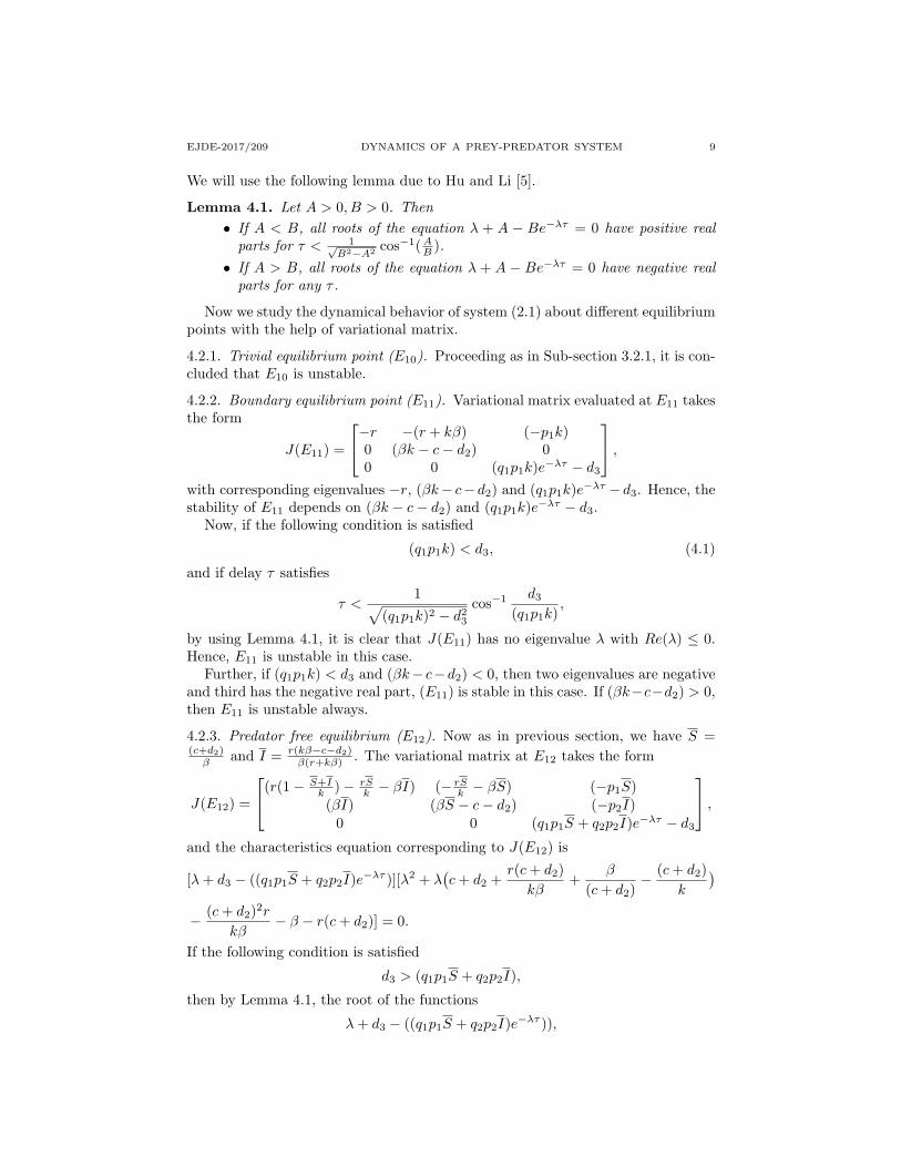
4.2.2. Boundary equilibrium point (E11). Variational matrix evaluated at E11 takesthe form

J(E11) =

−r −(r + kβ) (−p1k)0 (βk − c− d2) 00 0 (q1p1k)e−λτ − d3

,with corresponding eigenvalues −r, (βk− c− d2) and (q1p1k)e−λτ − d3. Hence, thestability of E11 depends on (βk − c− d2) and (q1p1k)e−λτ − d3.

Now, if the following condition is satisfied

(q1p1k) < d3, (4.1)

and if delay τ satisfies

τ <1√

(q1p1k)2 − d23

cos−1 d3

(q1p1k),

by using Lemma 4.1, it is clear that J(E11) has no eigenvalue λ with Re(λ) ≤ 0.Hence, E11 is unstable in this case.

Further, if (q1p1k) < d3 and (βk− c−d2) < 0, then two eigenvalues are negativeand third has the negative real part, (E11) is stable in this case. If (βk−c−d2) > 0,then E11 is unstable always.

4.2.3. Predator free equilibrium (E12). Now as in previous section, we have S =(c+d2)β and I = r(kβ−c−d2)

β(r+kβ) . The variational matrix at E12 takes the form

J(E12) =

(r(1− S+Ik )− rS

k − βI) (− rSk − βS) (−p1S)(βI) (βS − c− d2) (−p2I)

0 0 (q1p1S + q2p2I)e−λτ − d3

,and the characteristics equation corresponding to J(E12) is

[λ+ d3 − ((q1p1S + q2p2I)e−λτ )][λ2 + λ(c+ d2 +

r(c+ d2)kβ

+β

(c+ d2)− (c+ d2)

k

)− (c+ d2)2r

kβ− β − r(c+ d2)] = 0.

If the following condition is satisfied

d3 > (q1p1S + q2p2I),

then by Lemma 4.1, the root of the functions

λ+ d3 − ((q1p1S + q2p2I)e−λτ )),


will have negative real part for any value of τ and for the equation

λ2 + λ(

(c+ d2) +r(c+ d2)Kβ

+β

(c+ d2)− (c+ d2)

k

)+(− r(c+ d2)2

kβ− β − r(c+ d2)

)= 0,

the Routh-Hurwitz criteria, may be used for proving the fact that this equationwill have roots with negative real parts. Hence, if the equilibrium E12 is asymptot-ically stable, it will mean that predator population will be die-out from system soconsidered.

4.2.4. Infection free equilibrium (E13). S and Y are given by S = d3q1p1

, Y = [ rp1 (1−d3

kq1p1)]. The variational matrix at E13 takes the form

J(E13) =

(r(1− eSk )− rS

k − p1Y ) (− reSk − βS) (−p1S)

0 (βS − p2Y − c− d2) 0(q1p1Y e

−λτ ) (q2p2Y e−λτ ) (q1p1Se

−λτ − d3)

,One of the eigenvalue is (βS−p2Y −c−d2) and two other eigenvalues are the rootsof the expression[

λ2 − λ(r(1− 2S

k)− p1Y − d3 + (q1p1Y e

−λτ ))

+(−rd3(1− 2S

k)− d3p1Y

+ d3 + rq1p1S(1− 2Sk

)e−λτ)].

If the condition

S >(c+ d2 + p2Y )

β

is satisfied. Then one eigenvalue (βS − p2Y − c − d2) corresponding to J(E13) ispositive. Hence, in this case E13 is unstable. Let us put, λ = (u+iv) with conditionfor u as u ≥ 0 in the expression[

λ2 − λ(r(1− 2S

k)− p1Y − d3 + (q1p1Y e

−λτ ))

+(−rd3(1− 2S

k)

− d3p1Y + d3 + rq1p1S(1− 2Sk

)e−λτ)],

and on separating real and imaginary parts, we obtained

Real part = (u2 − v2)−(r(1− 2S

k)− p1Y − d3 + (q1p1Se

−λτ cos vτ)

+(rq1p1S(1− 2S

K)e−λτ cos vτ

),

Imaginary part = 2uv +(p1Y + d3 − vr(1−

2Sk

)− q1p1Se−λτ cos v

− uq1p1Se−λτ sin vτ − rq1p1S(1− 2S

k)e−λτ sin vτ

).


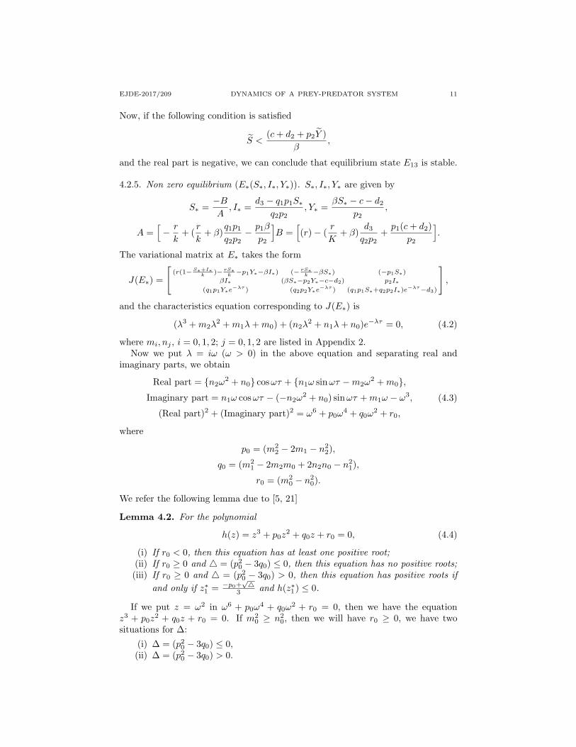
Now, if the following condition is satisfied

S <(c+ d2 + p2Y )

β,

and the real part is negative, we can conclude that equilibrium state E13 is stable.

4.2.5. Non zero equilibrium (E∗(S∗, I∗, Y∗)). S∗, I∗, Y∗ are given by

S∗ =−BA, I∗ =

d3 − q1p1S∗q2p2

, Y∗ =βS∗ − c− d2

p2,

A =[− r

k+ (

r

k+ β)

q1p1

q2p2− p1β

p2

]B =

[(r)− (

r

K+ β)

d3

q2p2+p1(c+ d2)

p2

].

The variational matrix at E∗ takes the form

J(E∗) =

[(r(1−S∗+I∗k )− rS∗k −p1Y∗−βI∗) (− rS∗k −βS∗) (−p1S∗)

βI∗ (βS∗−p2Y∗−c−d2) p2I∗(q1p1Y∗e

−λτ ) (q2p2Y∗e−λτ ) (q1p1S∗+q2p2I∗)e

−λτ−d3)

],

and the characteristics equation corresponding to J(E∗) is

(λ3 +m2λ2 +m1λ+m0) + (n2λ

2 + n1λ+ n0)e−λτ = 0, (4.2)

where mi, nj , i = 0, 1, 2; j = 0, 1, 2 are listed in Appendix 2.Now we put λ = iω (ω > 0) in the above equation and separating real and

imaginary parts, we obtain

Real part = n2ω2 + n0 cosωτ + n1ω sinωτ −m2ω

2 +m0,Imaginary part = n1ω cosωτ − (−n2ω

2 + n0) sinωτ +m1ω − ω3,

(Real part)2 + (Imaginary part)2 = ω6 + p0ω4 + q0ω

2 + r0,

(4.3)

where

p0 = (m22 − 2m1 − n2

2),

q0 = (m21 − 2m2m0 + 2n2n0 − n2

1),

r0 = (m20 − n2

0).

We refer the following lemma due to [5, 21]

Lemma 4.2. For the polynomial

h(z) = z3 + p0z2 + q0z + r0 = 0, (4.4)

(i) If r0 < 0, then this equation has at least one positive root;(ii) If r0 ≥ 0 and 4 = (p2

0 − 3q0) ≤ 0, then this equation has no positive roots;(iii) If r0 ≥ 0 and 4 = (p2

0 − 3q0) > 0, then this equation has positive roots ifand only if z∗1 = −p0+

√4

3 and h(z∗1) ≤ 0.

If we put z = ω2 in ω6 + p0ω4 + q0ω

2 + r0 = 0, then we have the equationz3 + p0z

2 + q0z + r0 = 0. If m20 ≥ n2

0, then we will have r0 ≥ 0, we have twosituations for ∆:

(i) ∆ = (p20 − 3q0) ≤ 0,

(ii) ∆ = (p20 − 3q0) > 0.


In situation (i), we have to say that E∗ is stable thus E∗ is absolutely stable if r0 ≥ 0and ∆ = (p2

0 − 3q0) ≤ 0 and also if we have and r0 ≥ 0 and ∆ = (p20 − 3q0) > 0

then equation has negative roots if and only if h(z∗1) > 0 where z∗1 = −p0+√4

3 , thuswe have the following theorem for the stability of E∗

Theorem 4.3. Equilibrium E∗(S∗, I∗, Y∗) is absolutely stable if one of the followingthree conditions holds

(i) ∆ = (p20 − 3q0) ≤ 0;

(ii) ∆ = (p20 − 3q0) > 0 and z∗1 = −p0+

√4

3 < 0;(iii) ∆ = (p2

0 − 3q0) > 0, z∗1 = −p0+√4

3 > 0 and h(z∗1) > 0 provided r0 ≥ 0.

Next if we consider the case when r0 < 0 or r0 ≥ 0,∆ = (p20 − 3q0) > 0, z∗1 >

0, h(z∗1) < 0. Then according to lemma 4.2, (4.3) will have one positive root sayω0 that is the characteristic equation has a pair of purely imaginary roots say ±iω0.Now assume that iω0, ω0 > 0 is a root of h(z). Solving the eq. (4.3) for τ , we have(by eliminating sinωτ , we obtain

τ =1ω0

cos−1(n1ω

20ω0 −m1 − m2ω

20 −m0n2ω

20 − n0

n21ω

20 + n2ω2

0 − n0) +

2kπω0

, (4.5)

for k = 0, 1, 2, . . . . We call it as a ‘critical value’ and is denoted by

τk =1ω0

cos−1(n1ω

20ω0 −m1 − m2ω

20 −m0n2ω

20 − n0

n21ω

20 + n2ω2

0 − n0) +

2kπω0

, (4.6)

for k = 0, 1, 2, . . . . This corresponds to the characteristic equation that has purelyimaginary roots ±iω0. Which is a result similar to that is discussed in [5]. Transver-sality condition may also obtained as discussed in [5]. As discussed in [5, Theorem2.4], the equilibrium point E∗ of the system (2.1) is asymptotically stable whenτ > τ0. τ = τk (k = 0, 1, 2, 3, . . . ) are Hopf-bifurcation values for the system (2.1)and τk is used as a point for direction of Hopf Bifurcation in next section.

Remark 4.4. From (4.5) and (4.6), it is observed that the delay term τ (herebifurcation parameter) depends on the values of mi, nj , i = 0, 1, 2; j = 0, 1, 2.Since mi, nj , i = 0, 1, 2; j = 0, 1, 2 depends on q1 and q2 (see Appendix 2), hencebifurcation parameter (τ) depends on q1 and q2 both. A little variation in the valuesof q1 and q2 may change the bifurcation parameter (τ). Hence, a little variation inthe values of q1 and q2 may change the dynamics of the delayed model (2.1).

5. Direction and stability of the Hopf Bifurcation

With the symbols used in [5] and the procedure explained in [12]. System (2.1),can be translated to the following functional differential equation (FDE) system

u(t) = Lµ(µt) + F (µ, ut), (5.1)

where ut = u(t) ∈ R3 and Lµ : R× C→ R3 and F : R× C→ R3 are given by,

Lµφ = (τk + µ)(M1φ(0) +M2φ(−1)),

F (µ, θ) =

− rkφ

21(0)− ( rk + β)φ1(0)φ2(0)− p1φ1(0)φ3(0)

βφ1(0)φ2(0)− p2φ2(0)φ3(0)q1p1φ1(−1)φ3(−1) + q2p2φ1(−1)φ2(−1)

,


where

M1 =

(r − 2rS∗k − ( rk + β)I∗ − p1Y∗) −( rk + β)S∗ (−p1S∗)

βI∗ (βS∗ − p2Y∗ − c− d2) −p2I∗0 0 −d3)

,M2 =

0 0 00 0 0

q1p1Y∗ q2p2Y∗ q1p1S∗ + q2p2I∗

,φ(0) = (φ1(0), φ2(0), φ3(0))T ∈ C,

φ(−1) = (φ1(−1), φ2(−1), φ3(−1))T ∈ C.

We have considered, τ = (τk +µ), µ = 0 which gives the Hopf bifurcation value forthe mathematical model with delay as promised in previous section. Normalizingdelay τ by the time scaling t → t

τ then the model is written in the Banach SpaceC ≡ C([−1, 0],R3).

By the Riesz representation theorem, we found that there exists a matrix functionwhose components are bounded variation function η(θ, µ) in θ ∈ [−1, 0], such thatLµφ =

∫Ωdη(θ, µ)φ(θ), φ ∈ C, Ω ∈ [−1, 0). We can choose

η(θ, µ) = (τk + µ)M1δ(θ)− (τk + µ)M2δ(θ + 1),

where δ(θ) denotes the dirac delta function viz.

δ(θ) =

0, θ 6= 0,1, θ = 0.

For φ ∈ C1([−1, 0],R3), we define

A(µ)φ(θ) =

dφ(θ)dθ , θ ∈ [−1, 0),∫ 0

−1dη(θ, µ)φ(θ), θ = 0,

=

dφ(θ)dθ , −1 ≤ θ < 0,∫ 0

−1dη(θ, µ)φ(θ), θ = 0.

and

R(µ)φ(θ) =

0, θ ∈ [−1, 0),F (µ, φ), θ = 0,

=

0, −1 ≤ θ < 0,F (µ, φ), θ = 0,

with these symbols, FDE system (5.1) may be written in the form

u(t) = A(µ)(µt) + R(µ)µt,

which is an abstract differential equation where ut(θ) = u(t+ θ),−1 ≤ θ < 0. Nowwe come to operator theory, for ψ ∈ C1

([0, 1], (R3)∗

)we define A∗, the adjoint

operator of A, by

A∗ψ(S) =

−dψ(S)

dS , S ∈ (0, 1],∫ 0

−1dηT (S, µ)ψ(−S), S = 0,


and a bilinear product

〈ψ(S), φ(θ)〉 = ψ(0)φ(0)−∫ 0

1

∫ θ

ξ=0

ψT

(ξ − θ)dη(θ)φ(ξ)dξ, (5.2)

where η(θ) = η(θ, 0). Then A(0) and A∗ are adjoint operators. From previoussection, it is noted that ±iω0τk are eigenvalues of A(0). Hence they are also theeigenvalues of A∗.

To determine the poincare normal form of the operator A, we first need to evalu-ate the eigenvectors of A(0) and A∗ corresponding to iω0τk and −iω0τk respectively.Suppose that q(θ) = (1, α1, α2)T exp(iω0τkθ) is the eigenvector of A(0) correspond-ing to iω0τk, then we have A(0)q(θ) = iω0q(θ) from the definition of A(0), wehave [

M1 +M2 exp(iω0τk)] 1

α1

α2

= iω0

1α1

α2

,or

M1

1α1

α2

+M2

exp(−iω0τk)α1 exp(−iω0τk)α2 exp(−iω0τk)

= iω0

1α1

α2

.By simple calculation, we obtain

α1 =−p2I∗(iω0 − (r − 2rS∗

K − ( rk + β)I∗ − p1Y∗))− p1βS∗I∗

p2( rk + β)S∗I∗ − p1S∗(iω0 − βS∗ + c+ d2 + p2Y∗),

α2 =q1p1Y∗ exp(−iω0τk + q2p2Y∗ exp(−iω0τk

iω0 + d3 − q1p1S∗ + q2p2I∗.

Next, suppose that q∗(s) = B(1, α∗1, α∗2) exp(iω0τks) is the eigenvector of A∗

corresponding to −iω0τk. Analogously, we have

α∗1 =−p1( rk + β)S∗ − p2(iω0 − (r − 2rS∗

k − ( rk + β)I∗ − p1Y∗))p2βI∗ − p1(iω0 + βS∗ − c− d2 − p2Y∗)

,

α∗2 =−p1S∗ − p2I∗α

∗1

−iω0 + d3 − (q1p1S∗ + q2p2I∗) exp(−iω0τk),

where B has to be calculated. We have the two conditions:

〈q∗, q(θ)〉 = 1, 〈q∗, q(θ)〉 = 0,

which may be verified. By equation (5.2), we have

〈q∗, q(θ)〉

= q∗(0)q(0)−∫ 0

−1

∫ ∞ξ=0

q∗T (ξ − θ)dη(θ)q(ξ)dξ

= B(1, α1∗, α2

∗)(1, α1, α2)T −∫ 0

−1

∫ ∞ξ=0

B(1, α1∗, α2

∗) exp(−iω0τk(ξ − θ))dη(θ)

× (1, α1, α2)T exp(iω0τkξ)dξ

= B1 + α1α1∗ + α2α2

∗ −∫ 0

−1

(1, α1∗, α2

∗) exp(iω0τk)dη(θ)(1, α1, α2)T

= B1 + α1α1∗ + α2α2

∗ + τk[q2p2α2∗Y∗ + q2p2α1α2

∗Y∗ + (q1p1S∗ + q2p2I∗)α2α2∗]

× exp(−iω0τk),


and

1 = B1 + α1α1∗ + α2α2

∗ + τk[q2p2α2

∗Y∗ + q2p2α1α2∗Y∗

+ (q1p1S∗ + q2p2I∗)α2α2∗] exp(−iω0τk),

which gives

B =(

1 + α1α1∗ + α2α2

∗ + τk[q2p2α2∗Y∗ + q2p2α1α2

∗Y∗

+ (q1p1S∗ + q2p2I∗)α2α2∗] exp(−iω0τk)

)−1

.

5.1. Stability of bifurcated periodic solutions. Firstly, we will investigate thecoordinates of the center manifold C0 at µ = 0. Let ut be the solution of (5.1)and define, z(t) = 〈q∗, ut〉, q∗ being the eigenvalue of A∗ and W (t, θ) = ut(θ) −2Rez(t)q(θ) on the Center Manifold C0, we have

W (t, θ) = W (z(t), z(t), θ),

where

W (z, z, θ) = W20(θ)z2

2+W02(θ)

z2

2+W11(θ)zz +W30

z3

b3+ . . . . (5.3)

In fact, z and z are local coordinates for the center manifold C0 in the direction ofq∗ and q∗ respectively. The existence of C0 will provide an opportunity to reducethe system u(t) = Lµ(ut) +F (µ, µt) into an ordinary differential equation ODE( ina single complex variable z) on C0 which is very interesting. ut is the solution ofsystem under consideration. ut ∈ C0, we have

z(t) = 〈q∗, ut〉= 〈q∗, A(ut) +R(ut)〉= 〈q∗, A(ut) > + < q∗, R(ut)〉= 〈A∗q∗, (ut) > + < q∗, R(ut)〉= iω0τz + q∗ · F (0,W (t, 0) + 2Re[z(t)q(θ)]).

We rewrite it asz(t) = iω0τz + g(z, z).

where

g(z, z) = g20(θ)z2

2+ g02(θ)

z2

2+ g11(θ)zz + g21

zz2

b3+ . . . .

The computation of coefficients of g(z, z) is done at Appendix 3.The coefficients g20, g02, g11 and g21 are used in calculating C0 etc. Since g21

(from Appendix 3) contains W20(θ) and W11(θ), we need to calculate them. Nowut = A(µ)ut + R(µ)ut and z(t) = 〈q∗, ut >, W (t, θ) = ut(θ)− 2Rez(t)q(θ) givesus

W = ut − zq − zq =

AW − 2Req∗(0)F0q(θ), −1 ≤ θ < 0,AW − 2Req∗(0)F0q(θ) + F0, θ = 0.

Rewriting the above equation, we obtain

W = AW +H(z, z, θ), (5.4)


where

H(z, z, θ) = H20(θ)z2

2+H11(θ)zz +H02(θ)

z2

2+H21(θ)

z2z

2+ . . . . (5.5)

Near the origin on C0, we have

W = Wz z +Wzz,

by (5.4) and (5.5), we have

(A− 2iω0τk)W20(θ) = −H20(θ),

AW11(θ) = −H11(θ),

hence for −1 ≤ θ < 0 we have

H(z, z, θ) = −2Re(q∗(0)F0q(θ)) = −g(z, z)q(θ)− g(z, z)q(θ).

By comparing the coefficients of z in H(z, z, θ), we have

H20(θ) = −g20q(θ)− g02q(θ),

H11(θ) = −g11q(θ)− g11q(θ).

Now, we have

W20(θ) = 2iω0τkW20(θ) + g20q(θ) + g02q(θ),

W11(θ) = g11q(θ) + g11q(θ).

On integrating, we have

W20(θ) =ig20

ω0τkq(0) exp(iω0τkθ) +

ig20q(0)3ω0τk

exp(−iω0τkθ) + E1 exp(2iω0τkθ),

W11(θ) =g21

iω0τkq(0) exp(iω0τkθ) +

ig11q(0)ω0τk

exp(−iω0τkθ) + E2,

where E1 and E2 are to be determined. From definitions of A, the equation (A −2iω0τk)W20(θ) = −H20(θ) gives us∫ 0

−1

dη(θ)W20(θ) = 2iω0τkW20(0)−H20(0),

which gives us

H20(0) = −g20q(0)− g02q(0) + 2τk

− rk − ( rk + β)α1 − p1α2

βα1 − p2α1α2

(q1p1α2 + q2p2α1) exp(−2iω0τk)

.Now, (

iω0τkI −∫ 0

−1

exp(iω0τkθ)dη(θ))q(0) = 0,(

− iω0τkI −∫ 0

−1

exp(−iω0τkθ)dη(θ))q(0) = 0.

We also have(2iω0τkI −

∫ 0

−1

exp(iω0τkθ)dη(θ))E1 = 2τk

− rk − ( rk + β)α1 − p1α2

βα1 − p2α1α2


,


which leads to a11 S∗( rk + β) p1S∗−βI∗ a22 p2I∗

−q1p1Y∗ exp(−2iω0τk) −q2p2Y∗ exp(−2iω0τk) a33

E1

= 2

− rk − ( rk + β)α1 − p1α2

βα1 − p2α1α2


,where

a11 = 2iω0 − (r − 2rS∗k− (

r

k+ β)I∗ − p1Y∗), a22 = 2iω0 − βS∗ + c+ d2 + p2Y∗,

a33 = 2iω0 + d3 − (q1p1S∗ + q2p2I∗) exp(−2iω0τk),

therefore,

E1 = 2

− rk − ( rk + β)α1 − p1α2

βα1 − p2α1α2


×

a11 S∗( rk + β) p1S∗−βI∗ a22 p2I∗


−1

.

(5.6)

provided a11 S∗( rk + β) p1S∗−βI∗ a22 p2I∗


is invertible.

Now,∫ 0

−1dη(θ)W11(θ) = −H11(0) and

H11(0) = −g11q(0)− g11q(0) + 2τk

− rk − ( rk + β)Re(α1)− p1Re(α2)βRe(α1)− p2Re(α1α2)

(q1p1Re(α2) + q2p2Re(α1)

,and hence this leads to the equation b11 S∗( rk + β) p1S∗

−βI∗ b22 p2I∗−q1p1Y∗ −q2p2Y∗ b33

E2 = 2



,where

b11 = (r − 2rS∗k− (

r

k+ β)I∗ − p1Y∗), b22 = −βS∗ + c+ d2 + p2Y∗,

b33 = d3 − (q1p1S∗ + q2p2I∗).

Then E2 can be obtained as

E2 = 2



b11 S∗( rk + β) p1S∗−βI∗ b22 p2I∗−q1p1Y∗ −q2p2Y∗ b33

−1

.

provided b11 S∗( rk + β) p1S∗−βI∗ b22 p2I∗−q1p1Y∗ −q2p2Y∗ b33


is invertible.By putting values of E1 and E2 we can obtain W20(θ) and W11(θ) and hence g21

is completely determined. Hence as stated in [12, 5], we can obtain the followingvalues:

c1(0) =i

2ω0τk(g11g20 − 2 | g11 |2 −

| g02 |2

3) +

g21

2,

µ2 = − Re(c1(0))Re(λ′(τk))

,

β2 = 2Re(c1(0)),

T2 = − 1ω0τk

[Im(c1(0)) + µ2 Im(λ′(τk))],

(5.7)

which determines the direction and stability of the model with delay at the criticalvalue τk. Now, we state the following main theorem of this section due to [5, 12, 6]

Theorem 5.1. (i) The sign of µ2 determined the direction of Hopf bifurcation.If µ2 > 0(µ2 < 0) , then the Hopf bifurcation is supercritical (sub critical).

(ii) The stability of bifurcated periodic solutions is determined by β2. The peri-odic solutions are stable if β2 < 0 and unstable if β2 > 0.

(iii) The period of bifurcated periodic solutions is determined by T2. The periodincreases if T2 > 0 and decreases if T2 < 0.

6. Numerical example

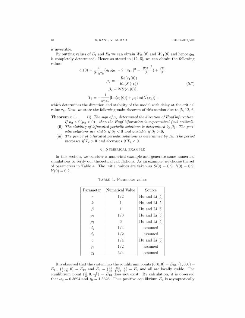
In this section, we consider a numerical example and generate some numericalsimulations to verify our theoretical calculations. As an example, we choose the setof parameters in Table 4. The initial values are taken as S(0) = 0.9, I(0) = 0.9,Y (0) = 0.2.

Table 4. Parameter values

Parameter Numerical Value Source

r 1/2 Hu and Li [5]

k 1 Hu and Li [5]

β 1 Hu and Li [5]

p1 1/8 Hu and Li [5]

p2 6 Hu and Li [5]

d2 1/4 assumed

d3 1/2 assumed

c 1/4 Hu and Li [5]

q1 1/2 assumed

q2 3/4 assumed

It is observed that the system has the equilibrium points (0, 0, 0) = E10, (1, 0, 0) =E11, ( 1

2 ,16 , 0) = E12 and E5 = ( 31

48 ,3531728 ,

76 ) = E∗ and all are locally stable. The

equilibrium point ( 43 , 0,

−43 ) = E13 does not exist. By calculation, it is observed

that ω0 = 0.3694 and τ0 = 1.5326. Thus positive equilibrium E∗ is asymptotically


stable when 0 < τ < τ0 = 1.5326. The system undergoes a Hopf bifurcation whensystem crosses through τ0. Few numerical simulations are represented by usingMATLAB.

It is observed from numerical simulations that the phase diagram of the systemchanges with slight changes in the initial values. First two figures (1 and 2) aredrawn for the value of τ = τ0 = 1.5326 and τ = 3.6249 > τ0 = 1.5326 respectively.From theoretical foundation it is observed that system is stable up to the criticalvalue of time delay τ . Critical value is calculated in (4.6). Beyond the critical valueof τ , Hopf bifurcation occurs. It is also observed in simulations. It is easy to seethat system undergoes Hopf bifurcation (See Figures 1 and 2). The simulations aretaken for the time interval [0, 1000] . For the simulation interval [0, 1000]. FromFigure 1, it is found that all the three populations are unstable with respect to time.Similar explanation is concluded from Figure 3. Figure 3 shows the stable natureof positive equilibrium which is drawn for τ = 1.1026 < 1.5326 = τ0, which is againconsistent with the theoretical formulation. Therefore, numerical simulations areconsistent with the theoretical formulation. If we choose the different set of valuesof the parameters q1 and q2 with the same other parameters and initial values, wemay have different figures (see Remark 3.2, 4.4).

7. Discussion and future directions

In the present study, we have considered an eco-epidemiological model withdisease in the prey population only. We have considered both cases with delayand without delay for analysis purpose. Local stability of all equilibrium pointshas been discussed. We have found the time delay as a game changer. This hasbeen observed that time delay τ may change the stability and even bifurcation mayoccur. Hopf-bifurcation analysis is presented, by the application of famous normalform theory, Riesz representation theorem and central limit theorem, stability anddirection of bifurcated periodic solutions have been investigated. Our analyticalresults has been compared with those in [5], when d2 = 0 and q1 = q2 = q.

Stability of the non zero (positive) equilibrium E5 indicates the existence andsurvival of all the three species in the ecosystem. Ecologically this equilibrium isvery important, because it provides actual interaction among all the three livingcomponents of the ecosystem. Actual balance is maintained under this situation.Ecologists are interested to observe the stability of non zero equilibrium point. It isalso remarkable that we classify our analysis in two parts (i) without delay (ii) withdelay. Ecologically, corresponding equilibrium points listed for our models (2.1) and(3.1) are same. For example, ecologically, E5 and E∗ are same but mathematicallyboth are different.

Theoretically, we can consider few examples of different ecosystems. If we con-sider Desert, Tundra, Savana geographical areas and consider an ecosystem fromthis area. Then positive equilibrium is more important, because in these areas manypredators are going to decline or decay because their prey are also facing naturalproblems like climate changes, lake of water, low quality of oxygen etc. and theyalso decaying, therefore in such geographical areas the predator population is notin position to catch their prey as they are limited and therefore they remain hungryfor most of the times, finally predator population starts decaying. For the ecologicalimbalance in such ecosystems, the main reason is the change in climate. Besidescutting of trees and global warming are also important environmental issues. Thus


0 200 400 600 800 1000−1

0

1

2

3

4

5Computed solution for the interval [0,1000]

time t

S,I,

Y

SIY

0.4 0.5 0.6 0.7 0.8 0.9 1−0.2

0

0.2

0.4

0.6

0.8

1

1.2Phase plane plot of susceptible prey (S) and infected prey(I)

S

I

−0.2 0 0.2 0.4 0.6 0.8 1 1.20

1

2

3

4

5Phase plane plot of infected prey (I) and predator (Y)

I

Y

0.4 0.5 0.6 0.7 0.8 0.9 10

1

2

3

4

5Phase plane plot of prey (S) and predator (Y)

S

Y

0.40.6

0.81

−0.5

0

0.5

10

1

2

3

4

5

S

3D Plot

I

Y

0 500 1000 1500 2000 25000.4

0.5

0.6

0.7

0.8

0.9

1Variation of healthy prey population with time

t

S

0 500 1000 1500 2000 2500−0.2

0

0.2

0.4

0.6

0.8

1

1.2Variation of infected prey population with time

t

I

0 500 1000 1500 2000 25000

1

2

3

4

5Variation of Predator Population with time

t

Y

Figure 1. Phase portrait of model with parameter values in Table4 with initial values S(0) = 0.9, I(0) = 0.9, Y (0) = 0.2

positive equilibrium can never exists, however if it exists, then not stable. If we con-sider hilly areas and consider an ecosystem from this area, then the cutting of treesand farming are two issues which are responsible for disturbance of climate in this


0 200 400 600 800 1000−1

0

1

2

3

4

5


time t

S,I,

Y

SIY

0.4 0.5 0.6 0.7 0.8 0.9 1−0.2

0

0.2

0.4

0.6

0.8

1


S

I

−0.2 0 0.2 0.4 0.6 0.8 1 1.20

1

2

3

4

5


I

Y

0.4 0.5 0.6 0.7 0.8 0.9 10

1

2

3

4

5


S

Y

0.40.6

0.81

−0.5

0

0.5

10

2

4

6

S

3D Plot

I

Y

0 500 1000 1500 20000.4

0.5

0.6

0.7

0.8

0.9


t

S

0 500 1000 1500 2000−0.2

0

0.2

0.4

0.6

0.8

1


t

I

0 500 1000 1500 20000

1

2

3

4

5


t

Y


area. In near past, one natural disaster in Uttarakhand (India) occurred, possiblybecause of cutting of trees and other developmental projects. This changed the cli-mate in hilly areas as well. This occurs the ecological imbalance in these areas and


0 20 40 60 80 100−1

0

1

2

3

4

5

6

7


time t

S,I,

Y

SIY

0.2 0.4 0.6 0.8 1−0.2

0

0.2

0.4

0.6

0.8

1


S

I

−0.2 0 0.2 0.4 0.6 0.8 1 1.20

1

2

3

4

5

6

7


I

Y

0.2 0.4 0.6 0.8 10

1

2

3

4

5

6

7


S

Y

0.20.4

0.60.8

−0.5

0

0.5

10

2

4

6

8

S

3D Plot

I

Y

0 100 200 300 4000.2

0.3

0.4

0.5

0.6

0.7

0.8

0.9


t

S

0 100 200 300 400−0.2

0

0.2

0.4

0.6

0.8

1


t

I

0 100 200 300 4000

1

2

3

4

5

6

7


t

Y


disturbs the natural ecosystems. Prey and predator both decays simultaneouslydue to unexpected mortality in the system. Thus if the positive equilibrium existsand is stable then the stability losses due to disaster. Similarly, if we choose the


aquatic ecosystem of any river in India, then the water pollution is a major factorin this ecosystem. Pollution disturbs the stability of the ecosystem and disturbs theecological balance. Positive equilibrium may loose stability in such ecosystems aswell. If we consider an ecosystem from green forest where pollution, weather con-ditions etc. are favorable for living species then actual prey-predation interactionwill be occurred. In this situation, if the positive equilibrium exists and is stablethis will provide the coexistence of all the three species. Thus equilibrium pointsE5 and E∗, if exists, are stable for an ecosystem from a forest area.

The parameters considered for numerical computation are purely imaginary andare suitably selected and are quite similar to result discussed in [5]. An attemptmay be done to estimate real parameters and these parameters may fit with thepresent mathematical model. This task may be achieved by real data collectionfrom field. Further, to study the model more scientifically, control strategies mayalso be investigated. This study may have applications with real ecosystems andbiomass available in the real world.

8. Appendix

Appendix 1: Ci, i = 1, 2, 3 of (3.6).

C1 = −(

(r − d2 − d3 − c) + S[−2rk

+ β + q1p1] + I[− rk

+ q2p2 − β]− Y (p1 + p2)),

C2 = S2[βq1p1 −2rq1p1

k− 2rβ

k] + Y 2[p1p2] + I2[(

r

k+ β)q2p2]

+ SI[βq2p2 −2rq2p2

k− (

r

k+ β)q1p1] + SY [−q1p1p2 − q1p

21 +

2rp2

k− p1β]

+ I Y [−q2p1p2 + (r

k+ β)p2] + S

[− βd3 − (c+ d2)q1p1 + rq1p1 +

2rd3

k

+ rβ +2r(c+ d2)

k

]+ I[− (c+ d2)q2p2 + rq2p2 + (

r

k+ β)d3 + (

r

k+ β)(c+ d2)

]+ Y

[d3p1 − rp2 + p1(c+ d2)

]+[d3(c+ d2)− rd3 − r(c+ d2)

],

C3 = −(S3[−2rq1p1β

k] + S2Y [

2rq1p1p2

k] + S2I[

2rq1p1p2

k] + I2Y [(

r

k+ β)q2p

22]

+ Y 2I[q2p22p1] + SIY

[− 2rq2p

22β

k+ 2(

r

k+ β)q1p1p2 − 2βq2p1p2

]+ S2

[βrq1p1 +

2rd3β

k+

2rq1p1(c+ d2)k

]+ I2[(

r

k+ β)q2p2(c+ d2)] + Y 2[d3p1p2]

+ SI[βrq2p2 +

2rq2p2(c+ d2)k

+ (r

k+ β)(c+ d2)q1p1

]+ SY [−rq1p1p2 +

2rp2d3

k+ d3βp1]

+ I Y[− rq2p

22 + (

r

k+ β)d3p2 + (c+ d2)q2p1p2

]


+ S[− d3rβ − r(c+ d2)q1p1 −

2r(c+ d2)d3

k

]+ I[− r(c+ d2)q2p2 − (

r

k+ β)(c+ d2)d3

]+ Y

[− d3p2r − (c+ d2)d3p1

]+ r(c+ d2)d3

).

Appendix 2: mi, nj, i = 0, 1, 2; j = 0, 1, 2 of (4.2).

m2 =(2rk

+p1β

p2− q1p1β

q2p2S∗

)+( rd3

q2p2k+ d3 −

p1(c+ d2)p2

− r),

m1 =(d3(c+ d2)− r(c+ d2)+ S∗−d3β +

2rkd3 + rβ +

2rk

(c+ d2)

+ I∗(r

k+ β)(d3 + c+ d2)+ Y∗d3p2 + d3p1 + (c+ d2)p1 + (r)p2

+ S2∗(−

2rβk

) + Y 2∗ (p1p2) + S∗Y∗(−βp1 +

2rKp2) + I∗Y∗(

r

k+ β)p2

),

m0 =(−r(c+ d2)d3 + S∗d3βr +

2rkd3(c+ d2)+ I∗d3(c+ d2)(

r

k+ β)

+ Y∗d3(c+ d2)p1 − rd3p2+ S2∗(−

2rkd3β) + Y 2

∗ (d3p2p1)

+ S∗Y∗−d3βp1 −2rkd3p2+ I∗Y∗(

r

k+ β)p2d3

),

n2 = −d3,

n1 =(S2∗q1p1β −

−2rkq1p1+ I2

∗−(r

k+ β)q2p2

+ S∗Y∗−q1p2p1+ S∗I∗q2p2β +2rkq2p2+ Y∗I∗−q2p2p1

+ S∗−(c+ d2)− rq1p1+ I∗−(c+ d2)q2p2 + rq2p2),

n0 = −(S2∗q1p1β(r − 2r

k) +

2rk

(c+ d2)q1p1 − q1p21β+ I2

∗(r

k+ β)(c+ d2)q2p2

+ S2∗Y∗

2rkq1p1p2 + q1p

21β+ S2

∗I∗−2rkq2p2β+ S∗I∗Y∗(

r

k+ β)q1p1p2

− 2βq2p1p2+ S∗Y∗−r + (r

k+ β)q1p1p2

+ S∗I∗βrq2p2 +2rk

(c+ d2)q2p2 + (c+ d2)(r

k+ β)q1p1

+ Y∗I∗(c+ d2)q2p2p1+ S∗(c+ d2)rq1p1+ I∗−(c+ d2)rq2p2).

Appendix 3. We have

g(z, z) = g20(θ)z2

2+ g02(θ)

z2

2+ g11(θ)zz + g21

zz2

b3+ . . . ,

g(z, z) = (q∗)TF (z, z)

= τkB(1, α∗1, α∗2)

− rku

21(t)− ( rk + β)u1(t)u2(t)− p1u1(t)u3(t)

βu1(t)u2(t)− p2u2(t)u3(t)p1q1u1(t− 1)(t)u3(t− 1) + p2q2u1(t− 1)u2(t− 1),


further, it is noticed that

u(t+ θ) = W (t, θ) + z(t)q(θ) + z(t)q(θ),

u1(t) = z + z +W (1)(t, 0),

u2(t) = α1z + α1z +W (2)(t, 0),

u3(t) = α2z + α2z +W (3)(t, 0),

u1(t− 1) = z exp(−iω0τk) + z exp(iω0τk) +W (1)(t,−1),

u2(t− 1) = α1z exp(−iω0τk) + α1z exp(iω0τk) +W (2)(t,−1),

u3(t− 1) = α2z exp(−iω0τk) + α2z exp(iω0τk) +W (3)(t,−1),

hence

g(z, z) = τkB[− rku2

1(t)− (r

k+ β)u1(t)u2(t)− p1u1(t)u3(t)

+ α1∗βu1(t)u2(t)− p2u2(t)u3(t)

+ α2∗p1q1u1(t− 1)(t)u3(t− 1) + p2q2u1(t− 1)u2(t− 1)],

putting the values of u1, u2, u3, u1(t − 1), u2(t − 1), u3(t − 1) etc. in g(z, z), weobtain

g(z, z) = τkB(− r

k[z + z +W (1)(t, 0)]2 − (

r

k+ β)[z + z +W (1)(t, 0)][α1z

+ α1z +W (2)(t, 0)]− p1[z + z +W (1)(t, 0)][α2z + α2z +W (3)(t, 0)]

+ α1∗(β[z + z +W (1)(t, 0)][α1z + α1z +W (2)(t, 0)]

− p2[α1z + α1z +W (2)(t, 0)][α2z + α2z +W (3)(t, 0)])

+ α2∗(p1q1[z exp(−iω0τk) + z exp(iω0τk) +W (1)(t,−1)]

× [α2z exp(−iω0τk) + α2z exp(iω0τk) +W (3)(t,−1)]

+ p2q2[z exp(−iω0τk) + z exp(iω0τk) +W (1)(t,−1)]

× [α1z exp(−iω0τk) + α1z exp(iω0τk) +W (2)(t,−1)])),

from this equation we can find the values of the coefficients g20(θ), g02(θ), g11(θ),g21(θ) etc. by comparing the same powers of z, we have

g20 = 2τkB−r

k− (

r

k+ β)α1 − p1α2 + βα1

∗α1 − α1∗α1α2p2

+ α2∗(p1q1α2 + p2q2α1) exp(−2iω0τk),

g11 = τkB(−2rk

+ (α1∗)β + α2

∗p2q2 −r

k+ β)(α1 + α1)

+ (α2∗p1q1 − p1)(α2 + α2)− α1

∗p2(α2α1 + α1α2)),

g02 = 2τkB−r

k− (

r

k+ β)α1 − p1α2 + βα1

∗α1 − α1∗α1α2p2

+ α2∗(p1q1α2 + p2q2α1) exp(2iω0τk),

g21 = 2τkB(− r

k(2W (1)

11 (0) +W(1)20 (0))− (

r

k+ β)[W (2)

11 (0) + α1W(1)11 (0)

+12α1W

(1)20 (0) +

12W

(1)20 (0)]− p1

[W

(3)11 (0) +

12W

(3)20 (0) + α2W

(1)11 (0)


+12W

(1)20 (0)

]+ α1

∗β[W (2)11 (0) +

12W

(2)20 (0) + α1W

(1)11 (0) +

12α1W

(1)20 (0)]

− α1∗p2[α1W

(3)11 (0) + α2W

(2)11 (0) +

12α2W

(2)20 (0) +

12α1W

(3)20 (0)]

+ α2∗p1q1[W (3)

11 (−1)e−iω0τk + α2W(1)11 (−1)e−iω0τk +

12W

(3)20 (−1)eiω0τk

+12W

(1)20 (−1)eiω0τk ] + α2

∗p2q2[W (2)11 (−1)e−iω0τk + α1W

(−1)11 e−iω0τk

+12W

(2)20 (−1)eiω0τk +

12W

(1)20 (−1)α1e

iω0τk ]).

References

[1] Berthier, K.; Langlais, M.; Auger, P.; Pontier, D.; Dynamics of a feline virus with two

transmission medels with exponentially growing host populations. Proc. Roy. Soc. Lond.3267 (2000): 2049–2056 http: //www.ncbi.nlm.nih.gov/pubmed/11416908

[2] Chattopadhyay, J.; Arino, O.; A predator-prey model with disease in prey. Non Linear Anal-

ysis 36 (1999): 747–766 http: //repository.ias.ac.in/7560/1/411.pdf[3] Haque, M; Zhen, J; Ventrino, E; An eco-epidemiological predator-prey model with stan-

dard disease incidence. Mathematical Methods in the Applied Sciences http: //dx.doi.org

/10.1002/mma.1071, 2008.[4] Hilker, F. M.; Schmitz, K.; Disease-induced stabilization of predator prey oscillations. Journal

of Theoretical Biology 255 (2008): 299–306 http: //dx.doi.org/10.1016/j.jtbi.2008.08.018

[5] Hu, G.-P.; Li, X.-L.; Stability and Hopf bifurcation for a delayed predator-prey modelwith disease in the prey. Chaos, Solitons and Fractals 45 (2012): 229–237 http:

//dx.doi.org/10.1016 /j.chaos.2011.11.011[6] Jana, S.; Kar, T. K.; Modeling and Analysis of a prey-predator system with disease

in the prey. Chaos, Solitons and Fractals 47 (2013): 42–53 http: //dx.doi.org/10.1016

/j.chaos.2012.12.002[7] De Jong, M. C. M.; et al; How does infection depend on the population size? in D. Mol-

lison(Ed.), Epidemic Models, their structure and Relation in data. Cambridge University

Press, 1994. http: //igitur-archive.library.uu.nl/vet[8] Greenhalgh, D.; Haque, M.; A predator-prey model with disease in the prey species only.

Math. Methods Appl. Sci. 30 (2007): 911–929. http: //dx.doi.org/10.1002/mma.815

[9] Kermack, W. O.; Mckendrick, A. G.; Contributons to the mathematical Theory of Epidim-ics, Part 1. Proc. Roy. Soc. A 115 (1927): 700–721 http: //rspa.royalsocietypublishing.org

/content/115/772/700.full.pdf+html

[10] Haque, M.; Venturino, E.; Increase of the prey may decrease the healthy prtedator popu-lation in presence of a disease in predator. HERMIS 7 (2006): 38-59 http: //www.aueb.gr/pympe/hermis/hermis-volume-7

[11] Litao, H.; Zhien, M. A.; Four Predator Prey Models with Infectious Diseases. Mathemati-cal and Computer Modeling 34 (2001): 849–858 http: //homepage.math.uiowa.edu/ heth-

cote/PDFs/2001MathCompMod.pdf[12] Karaaslanli, C. C.; Bifurcation Analysis and Its Applications, Chapter 1 in: Mykhaylo

Andriychuk (Ed.),Numerical Simulation: From Theory to Industry. (2012) 1-34 http://dx.doi.org/10.5772/50075

[13] Lotka, A.; Elements of Physical Biology. Williams and Wilkins, Baltimore.[14] Maoxing, L.; Zhen, J.; Haque, M.; An Impulsive predator-prey model with communicable

disease in the prey species only. Non Linear analysis: Real World Applications 10 (2009):3098–3111 http: //dx.doi.org/10.1016/j.nonrwa.2008.10.010

[15] Mukhopadhyaya, B.; Bhattacharyya, R.; Dynamics of a delay-diffusion prey-predator Modelwith disease in the prey. J. Appl. Math and Computing 17 (2005): 361–377 http://dx.doi.org/10.1007/BF02936062

[16] Naji, R. K.; Mustafa, A. N.; The Dynamics of an Eco-Epidemiological Model with Nonlinear

Incidence Rate. Journal of Applied Mathematics http: //dx.doi.org/10.1155/2012/852631,2012.


[17] Samanta, G. P.; Analysis of a delay nonautonomous predator-prey system with disease in the

prey. Non Linear Analysis: Modeling and Control 15 (2010): 97–108.

[18] Sophia Jang, R.-J.; Baglama, J.; Continous-time predator-prey models with parasites. J. Bio.Dyn 3 (2009): 87–98 http: //dx.doi.org/10.1080/1751375080228325

[19] Volterra, V.; Variazioni e fluttauazionidel numero d individui in species animals conviventii.

Mem Acd. Linciei (1926) 231–33.[20] Wang, F.; Kuang, Y.; Ding, C.; Zhang, S.; Stability and bifurcation of a stage-structured

predator-prey model with both discete and distributed delays, Chaos, Solitons and Fractals

46 ( 2013): 19–27 http: //dx.doi.org/10.1016/j.chaos.2012.10.003[21] Yanni, X.; Chen, L.; Modeling and analysis of a predator-prey model with disease in

the prey. Mathematical Biosciences 171 (2001): 59–82 http: /dx.doi.org/10.1016/S0025-

5564(01)00049-9[22] Yang, K.; Delay differential equations with applications in population dynamics. Academic

Press, INC., 1993.

Shashi KantDepartment of Applied Mathematics, Delhi Technological University, Delhi 110042,

India

E-mail address: [email protected]

Vivek Kumar

Department of Applied Mathematics, Delhi Technological University, Delhi 110042,India

E-mail address: vivek [email protected]

dynamics of a prey-predator system with infection in … · dynamics of a prey-predator system with...

Documents