dynamics of a control theory ordering system · 2018-01-09 · dynamics of a control theory...
TRANSCRIPT

DYNAMICS OF A CONTROL THEORY ORDERING
SYSTEM
SOUIADE MEHDI DAMIEN
NATIONAL UNIVERSITY OF SINGAPORE
2007

DYNAMICS OF A CONTROL THEORY ORDERING SYSTEM
SOUIADE MEHDI DAMIEN
A THESIS SUBMITTED
FOR THE DEGREE OF MASTER OF ENGINEERING
DEPARTMENT OF INDUSTRIAL & SYSTEMS ENGINEERING
NATIONAL UNIVERSITY OF SINGAPORE
2007

i
Acknowledgment
I would like to express my sincere appreciation and gratitude to my supervisors,
Doctor Wikrom Jaruphongsa and Associate Professor Chew Ek Peng, for their ad-
vice, guidance and assistance throughout the course of this project. I came to them
with a subject they were not much familiar with, and they showed an interest and
an openmindedness which motivated me all over my work. I benefited from this
relationship and hope they did in return.
I would also like to thank the administration of the ISE department, especially
Ow Lai Chun who helped me a lot, Victor, the laboratory officer as well as my lab-
mates. The latters made the “computer lab” a nice place to work and live in. More
importantly, we shared interesting ideas on our relative works, which undoubtedly
have added value to my work. I am especially grateful to Wei Wei and Long Quan.
I would like to extend this acknowledgement to all my friends who have been with
me one way or another during this time, in Singapore (Philippe, Fred, TingTing,
Robin, JC, Lisa, Yurou, Alexis, Charlotte, FongTien and the Latinis) or thousand
kilometers away (Jb, Xavier, Remy, Nico, Thomas, Tracy, Karine).
Finally and most importantly, I thank my parents and my sister for their contin-
uous help and for the love they have always showed me. This work would not exist
had they not supported me the way they did.
April 27, 2007
ii
Name : Souiade Mehdi Damien
Degree : Master of Engineering
Supervisor(s) : Doctor Wikrom Jaruphongsa, Associate Professor Chew Ek Peng
Department : Department of Industrial & Systems Engineering
Thesis Title : Dynamics of a control theory ordering system
Abstract
The supply chain performance has become a key success factor in today’s compet-
itive business environment. This study aims at considering its core element-the
ordering policy. The emphasis is carried upon the behaviour of the system in a dy-
namic environment. As a consequence, we use control theory grounds to define and
analyse our system. The bullwhip effect and the flexibility are the two main con-
cepts we focus on. They epitomize a tradeoff common to quite a number of systems,
that is being flexible without costing too much. To quantify these two concepts,
we adopt different dynamic approaches and define new metrics. The profit issue is
also introduced as a third dimension. In this study, supply chain managers will find
an intuition-builder as well as a quantitative-oriented analysis which can help them
make more consistent decisions.
Keywords : systems dynamics, ordering policy, flexibility, bull-
whip effect, lead time, profit, control theory
Contents
1 Introduction 1
1.1 The general approach and motivation . . . . . . . . . . . . . . . . . 1
1.2 Overview of the study and contribution . . . . . . . . . . . . . . . . 4
2 Literature review 6
2.1 The modeling methodology . . . . . . . . . . . . . . . . . . . . . . . 6
2.1.1 What is control theory? . . . . . . . . . . . . . . . . . . . . . 6
2.1.2 A striking example of how dynamics are important . . . . . . 10
2.2 Literature of control theory related to inventory management . . . . 15
2.2.1 The forerunners . . . . . . . . . . . . . . . . . . . . . . . . . . 15
2.2.2 The bullwhip effect . . . . . . . . . . . . . . . . . . . . . . . . 17
2.2.3 The flexibility . . . . . . . . . . . . . . . . . . . . . . . . . . . 19
2.2.4 The latest applications of control theory . . . . . . . . . . . 21
2.3 Systems dynamics and supply chains . . . . . . . . . . . . . . . . . . 25
3 Description of the model 28
3.1 The ordering policy model . . . . . . . . . . . . . . . . . . . . . . . . 28
3.1.1 The basic model . . . . . . . . . . . . . . . . . . . . . . . . . 28
3.1.2 Comparison with the traditional base-stock policy . . . . . . 37
iii

CONTENTS iv
3.1.3 Introduction of the possibility of shortages . . . . . . . . . . . 37
3.1.4 Initialisation . . . . . . . . . . . . . . . . . . . . . . . . . . . 38
3.1.5 Final model . . . . . . . . . . . . . . . . . . . . . . . . . . . . 39
3.2 Simulations . . . . . . . . . . . . . . . . . . . . . . . . . . . . . . . . 41
3.3 Introduction of the profit into the model . . . . . . . . . . . . . . . . 45
4 Control theory tools 49
4.1 A fundamental result on linear systems . . . . . . . . . . . . . . . . . 49
4.2 The z-transform . . . . . . . . . . . . . . . . . . . . . . . . . . . . . 50
4.3 Transfer functions . . . . . . . . . . . . . . . . . . . . . . . . . . . . 51
4.4 Stability . . . . . . . . . . . . . . . . . . . . . . . . . . . . . . . . . . 52
4.5 The Tsypkin Theorem . . . . . . . . . . . . . . . . . . . . . . . . . . 53
5 Analysis of the ordering policy 54
5.1 Transfer functions of the ordering policy . . . . . . . . . . . . . . . . 55
5.1.1 Deriving the order, work-in-process and net stock transfer
functions . . . . . . . . . . . . . . . . . . . . . . . . . . . . . 55
5.1.2 Stability of the system . . . . . . . . . . . . . . . . . . . . . . 58
5.2 A frequency approach to the bullwhip effect . . . . . . . . . . . . . . 61
5.2.1 Bode diagrams . . . . . . . . . . . . . . . . . . . . . . . . . . 61
5.2.2 Independent and identically distributed demand . . . . . . . 65
5.3 A time approach to the system’s characteristics . . . . . . . . . . . . 72
5.3.1 The order step response . . . . . . . . . . . . . . . . . . . . . 72
5.3.2 The step responsiveness metric . . . . . . . . . . . . . . . . . 76
5.3.3 The step bullwhip effect metric . . . . . . . . . . . . . . . . . 76
5.3.4 The step adaptability metric . . . . . . . . . . . . . . . . . . 78

CONTENTS v
5.4 Understanding and compromising the bullwhip effect and the flexibility 82
5.5 Effect of the lead time . . . . . . . . . . . . . . . . . . . . . . . . . . 85
5.5.1 Lead time and Bode diagrams . . . . . . . . . . . . . . . . . . 85
5.5.2 Lead time and independent and identically distributed demand 87
5.5.3 Lead time and step response . . . . . . . . . . . . . . . . . . 89
5.6 The profit issue . . . . . . . . . . . . . . . . . . . . . . . . . . . . . . 90
5.6.1 Profit and independent and identically distributed demand . 90
5.6.2 The profit step response . . . . . . . . . . . . . . . . . . . . . 91
6 Conclusion 96

List of Figures
2.1 Inventory versus Time . . . . . . . . . . . . . . . . . . . . . . . . . . 12
2.2 Block Diagram . . . . . . . . . . . . . . . . . . . . . . . . . . . . . . 23
2.3 Timeframe . . . . . . . . . . . . . . . . . . . . . . . . . . . . . . . . . 24
3.1 Basic production-inventory model . . . . . . . . . . . . . . . . . . . . 29
3.2 The different variables along the timeline . . . . . . . . . . . . . . . 33
3.3 Ordering Policy . . . . . . . . . . . . . . . . . . . . . . . . . . . . . . 36
3.4 Final Ordering Policy Model . . . . . . . . . . . . . . . . . . . . . . 40
3.5 Simulation 1: the Demand (no shortage) . . . . . . . . . . . . . . . . 42
3.6 Simulation 1: NS, WIP and Orders (no shortage) . . . . . . . . . . . 42
3.7 Simulation 2: the Demand (two shortages) . . . . . . . . . . . . . . . 43
3.8 Simulation 2: NS, WIP and Orders (two shortages) . . . . . . . . . . 43
3.9 The ordering policy model . . . . . . . . . . . . . . . . . . . . . . . . 46
3.10 Simulation 1: the cash flows . . . . . . . . . . . . . . . . . . . . . . . 47
3.11 Simulation 2: the cash flows (shortage) . . . . . . . . . . . . . . . . . 48
5.1 Bode diagram in amplitude relative to the orders . . . . . . . . . . . 62
5.2 Bode diagram in amplitude relative to the orders, no bullwhip effect
reduction possible . . . . . . . . . . . . . . . . . . . . . . . . . . . . 63
vi

LIST OF FIGURES vii
5.3 Effect of the proportional controllers . . . . . . . . . . . . . . . . . . 63
5.4 An example of seasonal bullwhip effect . . . . . . . . . . . . . . . . . 64
5.5 Bullwhip effect metric for i.i.d demand . . . . . . . . . . . . . . . . . 71
5.6 Step responsiveness metric . . . . . . . . . . . . . . . . . . . . . . . . 77
5.7 Step bullwhip effect metric . . . . . . . . . . . . . . . . . . . . . . . 78
5.8 Comparison of Net Stock answers to an aggressive and a smooth or-
dering policies . . . . . . . . . . . . . . . . . . . . . . . . . . . . . . . 80
5.9 Comparison of WIP answers to an aggressive and a smooth ordering
policies . . . . . . . . . . . . . . . . . . . . . . . . . . . . . . . . . . 80
5.10 Comparison of Orders answers to an aggressive and a smooth ordering
policies . . . . . . . . . . . . . . . . . . . . . . . . . . . . . . . . . . 81
5.11 The step adaptability metric . . . . . . . . . . . . . . . . . . . . . . 81
5.12 Bullwhip effect, responsiveness, adaptability: compromising . . . . . 84
5.13 Effect of the lead time on the orders . . . . . . . . . . . . . . . . . . 86
5.14 Effect of the lead time on the iid bullwhip effect metric with α = 0.1 88
5.15 Effect of the lead time on the iid bullwhip effect metric with α = 0.2 88
5.16 Effect of the lead time on the iid bullwhip effect metric with α = 0.3 89
5.17 Cash Flow response to a unit step in demand with different adjusting
times . . . . . . . . . . . . . . . . . . . . . . . . . . . . . . . . . . . 92
5.18 Net Stock response to a unit step in demand with different adjusting
times . . . . . . . . . . . . . . . . . . . . . . . . . . . . . . . . . . . 93
5.19 Orders response to a unit step in demand with different adjusting
times . . . . . . . . . . . . . . . . . . . . . . . . . . . . . . . . . . . 93
Chapter 1
Introduction
1.1 The general approach and motivation
Today’s market characteristics have forced companies to invest more in their sup-
ply chains. Increased competition among companies as well as higher customers’
expectations have led companies to improve their supply chain. It has also been
recognized that supply chains have become key drivers to financial performance.
These improvements range from new management techniques to more efficient tools
enabled by communication and transportation technologies.
According to Simchi-Levi et al.[1], Supply Chain Management (SCM) is ‘a set of
approaches used to efficiently integrate suppliers, manufacturers, warehouses, and
stores so that merchandise is produced and distributed at the right quantities, to
the right locations, and at the right time in order to minimize systemwide costs
while satisfying service-level requirements’. Thus, the highest stake in SCM is to
determine strategies and processes which comply with these requirements.
1

CHAPTER 1. INTRODUCTION 2
As we can feel through that definition, companies no longer consider the supply
chain only as the means of distributing the products to the customers; they now re-
gard it as a way of addressing and satisfying the customer sevice-level requirements.
This new approach may also be apprehended by examining how different the con-
siderations were in the past (see [2]). At the time of supply-driven manufacturing,
what first mattered was to deliver to the customers products with no defects. The
companies measured their efficiency mainly through internal performance indica-
tors and quality controls. Now, as the markets have become more customer-driven,
the quality of the products is still fundamental but they try to better understand
the customers’ behaviors which make them choose a product over another one. It
appears that the overall supply chain efficiency can make the difference between
different products.
In order to increase their supply chain efficiency, companies have to deal with
two main problems. The first one is matching the market characteristics. What
is the utility of a supply chain which can deliver a product overnight whereas the
customer would have prefered it at a lower price, accepting a longer delivery time?
The question of what customers actually value has become the central question and
a supply chain must be designed for that purpose. Supply chain designs have to take
into account the market they address and not only concentrate on internal optima.
And these markets continuously evolve, they change over time, they are dynamic.
And this is all the more relevant nowadays as the competitiveness has increased.
This consideration embraces a more general issue which is the relationship of a sup-
ply chain with its dynamical environment. With regards to the evolution with time,
new concepts have emerged, such as the flexibility. The question of the flexibility
CHAPTER 1. INTRODUCTION 3
of the supply chain system has become fundamental in the sense that there is a
growing need for adaptability and responsiveness to the environment evolution. At
first sight, these concepts can seem abstract and one of our objectives in this study
is to give them rigorous, precise and more practical meaning.
The second issue a good supply chain should tackle is the bullwhip effect. This
effect is the increase in demand variability of the orders when we go upstream the
chain, from the retailers to the raw material suppliers. Several papers tackle this
problem and give advice to impede it as much as possible, because it has a detrimen-
tal impact on the supply chain performance. Demand forecasting, ordering policy
and the presence of lead times are among three of the main factors contributing to
this effect.
Actually, a third dimension that should also be considered is cost. It is generally
taken for granted that cost is the most important parameter used to determine the
efficiency of a supply chain. Supply chain designers cannot be satisfied with systems
the only aim of which is to distribute the products at the lowest cost possible. The
supply chain must now be seen as a product enhancer which interacts with the
customers. Today, customers demand higher-quality products and quicker delivery,
at a low price. Although the cost is still a major parameter to optimize, it should
be put into perspective with other parameters which take into account modern
requirements that participate to the price formation, ultimately determined by the
customers’ perception of the value added by the product and/or service.
Consequently, and to be more explicit, flexibility and systemwide costs should
be considered altogether to achieve top performance.

CHAPTER 1. INTRODUCTION 4
1.2 Overview of the study and contribution
In order to get insights on the issues mentioned, we will study the dynamics of an
ordering policy. To do so, we will use the theoretical framework of control theory
because of its relevance to the problem as we will see.
More and more, the management policies tend to coordinate as much as possible
the different systems contributing to the success of the company. Given the com-
plexity of a company, this is very challenging and it requires understanding the role
played by every part of the system as well as the interaction between those parts.
The tradeoffs at stake, which we will point out along the study, are also important
to understand in order to make more informed decisions.
In the literature review (chapter 2), we explain the motivation for the use of this
theory and we present the literature of control theory applied to inventory manage-
ment. We also review the concepts of flexibility and bullwhip effect. To conclude,
the systems dynamics approach is described and its relevance to our study is formu-
lated.
The first part of the study (chapter 3) consists of defining a single-stage model of
the ordering policy. The modeling phase is important because it is the formalization
of our understanding of the system.
In chapter 4, we introduce a few theoretical concepts that are used for the anal-
ysis of the system. The purpose is to make the reader familiar with some control
theory concepts and tools.
Then in chapter 5, we start the proper analysis of the system in order to work
out some useful properties. We focus on the dynamics of the system including flex-
ibility, bullwhip effect and profit issues.

CHAPTER 1. INTRODUCTION 5
This study aims at understanding the dynamics of an ordering policy. Our contri-
butions are many folds. Firstly, we come up with a simulation model of our system.
This simulation model can be used for educational purpose for those interested in
such ordering policy modeling. Secondly, we perform an analysis of this system with
an emphasis on the dynamics of the system, with an instrumental role played by the
lead time. We also study the response of the system to different demand patterns,
which enhances the comprehension of the bullwhip effect phenomenon. Thirdly, we
define new metrics relative to the bullwhip effect and the flexibility and highlight
the tradeoff at stake between these two concepts. From our point of view, this last
point represents our main contribution. We have used a scientific approach and
defined quantitative means to tackle the flexibility concept which may be seen as
rather qualitative. We hope this contribution will help in the better understanding
of the ordering system, the core of a supply chain system.

Chapter 2
Literature review
We first introduce the important concepts that support our study and explain why
we use control theory as a modeling technique. These concepts are the dynamics of
supply chain systems, the use of feedback and the importance of the inherent lead
time. Then we review the literature relating this theory to inventory management.
At the same time, we introduce two fundamental concepts which are the bullwhip
effect and the flexibility. We conclude with a talk about the complexity that arises
in supply chain systems and how a systems thinking approach enhances our under-
standing.
2.1 The modeling methodology
2.1.1 What is control theory?
The main idea which supports our modeling technique is that supply chains are
dynamic systems. They are systems which evolve over time. Our belief is that
models which consider the supply chain from a static point of view cannot catch
6

CHAPTER 2. LITERATURE REVIEW 7
one of its essential features, its evolution along time which has become a central
issue in today’s business environment. By definition, the most appropriate method
to study dynamic systems is control theory. Indeed, control theory is the study of
such time-varying systems and of the differential equations which govern them: the
modeling, the analysis and the control of such systems are the three components of
this field.
Control Theory or Automatic Control has been used since the beginning of the
20th century. Some of its concepts already existed but it really appeared as a field
in itself at that time. Nowadays, the fields of application are numerous and lie from
robotics and manufacturing to economics. It is also applied to design or model inven-
tory policies. A good review of the application of control theory to the production-
inventory problem is presented by Ortega and Lin in [3]. Some of the ideas developed
hereafter are inspired from this work.
What is a system?
Any system is defined as a combination of different parts which coordinate in order
to produce a result, to make a determined function (see [4]). The different parts may
be interdependent in the sense that they influence each other. A supply chain is a
system comprising interdependent parts such as the level of stock and the inventory
policy. This interdependency is explained by the following scheme: a low stock level
will imply high orders to replenish the stock, which will induce a higher (and pos-
sibly too high) stock level, which will induce lower orders in return. The thorough
understanding of these interdependencies is a key to mastering complex systems.

CHAPTER 2. LITERATURE REVIEW 8
In order to study a system, we can model it. Any model is aimed at reproducing
what happens in the real world. As a consequence, it is used to comprehend the
real world in order to domesticate it better. When modeling, one should keep in
mind that any model reflects the understanding of the system from the modeler’s
point of view, so much so that two different people will most probably come up with
two different models for the same considered system. A map models a territory, but
the map is not the territory, and two different persons would certainly produce two
different maps of the same territory. As a consequence, the modeling process is fun-
damental since it allows people to understand how the one who has built the model
understands the system, models the territory. Our model is one representation of
the real world ordering policy.
The feedback
In Control Theory, one of the fundamental concepts to understand is the feedback.
It is the tool to model interdependency. To explain what it is, let us first emphasize
the fact that automatic systems copy the human behavior and see how the human
behavior uses feedback. For that purpose, let us analyze what a car driver’s behavior
consists of.
• First, he observes the characteristics of his car: the speed, the position,...; as
well as the environment: a car ahead which brakes, a turning,...
• Then, he analyses the data he has just observed and acts on the steering wheel
and the pedals to change the characteristics of the car.
• Finally, he goes back to the observation of the new characteristics of the car

CHAPTER 2. LITERATURE REVIEW 9
and repeats the process.
An automatic system works the same way. The last stage is the feedback : the new
characteristics are observed and used to define the new command to apply to the
system. Everyday, the feedback is used to make decisions. For instance, stock man-
agers check the level of their stock, collect information about the environment and
afterwards decide on how much to order. It is important to understand this concept
and its consequences on the policies we implement. Control theory does provide a
theoretical framework for rigorously modeling feedbacks which we will exploit.
To come back to the current business environment, and in order to succeed in this
business environment, companies need to adopt a customer-driven approach, which
simply means that they use the feedback given by the customers to its products and
messages.
Complex dynamic systems
The old factory-driven, push model of the 20th century has seen its age. Nowadays,
the business environment is dynamic and complex in the sense that it changes over
time, contains nonlinearities, inertia, delays and networked feedback loops. The
supply chain has to show capabilities against this ever-changing environment. This
is the second point that supports our methodology choice. Control theory enables
modeling these complex dynamic systems, even if the difficulty may lie in getting
analytical results given such a complexity. Supply chains are complex dynamic sys-
tems which interact with complex dynamic markets. Time really is a fundamental
dimension which we want to give the highest importance. Stalk [5] wrote an award-
winning article in 1988 stating the importance of time as a strategic weapon. Its

CHAPTER 2. LITERATURE REVIEW 10
main idea is that an organization that eliminates wasted time in manufacturing,
services, new-product development, and sales and distribution will cut costs, serve
customers better, reduce inventories, and enhance innovation. It may not seem to be
such a revolutionary idea, but thoroughly understanding how time affects a system’s
performance proves to be a key success factor in the 21st century business environ-
ment where technological progress and globalization nurture intense competition.
The supply chains have to respond and adapt quickly to these changes if they want
to remain competitive.
Control theory provides a theoretical framework to model, and consequently
better understand complex and dynamic systems. As a consequence, it proves very
relevant to use this theory in our study to model and analyze these complex systems
of supply chains.
2.1.2 A striking example of how dynamics are important
Let us consider a first simple model which illustrates the dynamic behavior of supply
chains. It is inspired from the work of Sterman and the reader can refer to his book
‘Business Dynamics’ (see [6]). This example should also ring a bell to those familiar
with ‘the beer game’. We decided to present this example because it allows us to
introduce the importance of the lead time. It is a single-stage system the variables
of which are the inventory on hand I(t), the receiving rate R(t) and the demand
rate D(t). Time is defined as a continuous variable in general, but becomes discrete
when it comes to simulation for obvious reasons. The order rate O(t) is received
with a time delay corresponding to the lead time τ so that we have:
O(t− τ) = R(t).
CHAPTER 2. LITERATURE REVIEW 11
The differential equation which rules the system is:
dI(t)dt
= R(t)−D(t) = O(t− τ)−D(t). (2.1)
It is important to notice that the natural way to model dynamic systems is to use
differential equations. We recall that, by definition, control theory is the field which
studies the dynamics of physical systems ruled by differential equations.
The question is to know how much to order given some target performance. Let
us assume that the system is well balanced until time t1 with constant demand
D(t) = c1:
for t < t1, R(t) = O(t− τ) = D(t),
so that I(t) is constant. What if for t > t1, there is a step in the demand function:
D(t) = c1 +∆? Such an upswing change can result from an advertising campaign or
a favorable report from a famous analyst; on the other hand, a competitor’s product
price decrease may imply a downswing step. Whatever the reason is, the result on
the stock level of this unexpected change depends on the ordering policy. Let us
assume that the ordering policy consists of setting a target level for the inventory
and to order proportionally to the difference between the inventory and the target
inventory level:
O(t) = TargetLevel − I(t).
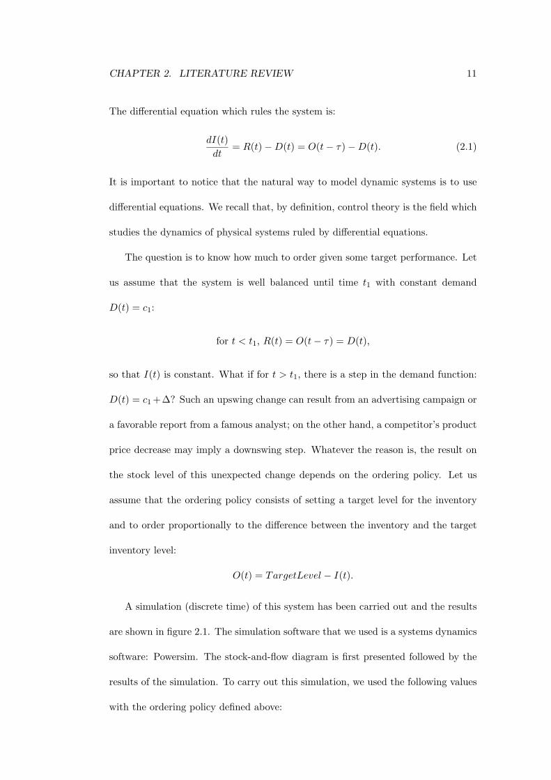
A simulation (discrete time) of this system has been carried out and the results
are shown in figure 2.1. The simulation software that we used is a systems dynamics
software: Powersim. The stock-and-flow diagram is first presented followed by the
results of the simulation. To carry out this simulation, we used the following values
with the ordering policy defined above:

CHAPTER 2. LITERATURE REVIEW 12
Figure 2.1: Inventory versus Time
• Lead Time = 2
• Demand=20 if t ≤ 10; Demand=22 otherwise, that is t ≥ 11
• Target Level=50 which can be seen as the sum of the single-period demand of
20 and of a safety stock of 30
As we can see from figure 2.1, the result is amplified oscillations which we easily
figure out how detrimental they are for the overall efficiency of the system. This
interesting result is not that obvious at first sight.
Let us try to understand what happens. Even if it can seem quite tedious, it is
very interesting to go deeply through this to understand the dynamical behaviour
of this system, and the role played by the lead time. The discrete time formula to
calculate the inventory level is:
I(t+ 1) = I(t) +R(t+ 1)−D(t+ 1).
Until period 10, everything is well balanced: the demand rate equals the receiv-
ing rate and the inventory level stays sticked to its assigned target level. At period
CHAPTER 2. LITERATURE REVIEW 13
11, the demand passes to 22 instead of 20. Thus, the inventory level begins to de-
plete because the receiving rate is still equal to the orders made when the inventory
level was constant, which means that the receiving rate is still 20 (we recall here
that the receiving rate is the order rate delayed by the lead time). So the depletion
rate is 2 units per time period.
At period 11, the inventory level is thus 28. The order changes from 20 to
50−281 = 22 but this order will only be received at the beginning of period 14,
R(14) = 22. We need to be aware that the order is made at the end of the pe-
riod, so an order made at the end of period t is received at the beginning of period
t+ 1 + leadtime. In the same way, at the end of period 12, the inventory level is 26
and an order of 24 is made the corresponding units of which will be received at the
beginning of period 15, R(15) = 24.
At period 13, the inventory still goes down to 24. We receive 20 units and the
demand is also 22. We order 26 units, R(16) = 26.
At period 14, the inventory keeps constant equal to 24 since the demand rate
and the receiving rate are the same and equal to 22. We order 26, R(17) = 26.
At period 15, the inventory goes up to 26 since we receive 24 units (more than
needed to only fulfill the demand) and the demand is still equal to 22. We order 26.
The fundamental fact is that we have entered a phase during which what we receive
exceeds the demand.
At period 16, the inventory goes up to 30 and continues up to 34 at time 17.
We are now beyond the target level but we are still receiving more than needed. It
contributes to worsen the situation and explains the overshoot, and the collapse
afterwards. The elements that explain the collapse are the same as the ones that
explain the overshoot, the difference being that we receive less than needed.
CHAPTER 2. LITERATURE REVIEW 14
What is important to remember from that example is that there are changeovers
between periods during which what we receive exceeds what we sell and vice versa.
This system is a closed-loop system in the sense that it is a feedback loop which
determines the ordering policy. The output of the system (the inventory) is com-
pared with the input (the target level) and their difference is fed back into the system
to alter the output in order to reduce the difference. This mimics human’s behavior
in front of such stock management situation. At first sight, we could think that
the ordering policy is consistent and may give acceptable results; we set a target
level and we order the difference between the inventory level and this target level in
order to stay close enough to the target level. But it proves totally inefficient with
amplified oscillations. The main explanation is the presence of a lead time. The lead
time is an essential component of the dynamic complexity of a supply chain system
and should always be taken into account in the modeling process of supply chains.
Control theory enables the lead time to be considered in the model and will help us
get insights on how to domesticate its effects.
Let us now have a look in the past and see what the applications of this theory
to supply chain problems have been until today.

CHAPTER 2. LITERATURE REVIEW 15
2.2 Literature of control theory related to inventory
management
2.2.1 The forerunners
In an article published in 1952, Simon [7] was the first one to show the applicability
of what was called ‘servomechanism theory’ to production control problems. He first
described the heat regulation of a closed space as an example of controlled system:
the difference between the target temperature and the current temperature is fed
back into the system and appropriate action (warm or cool the room) is taken. He
then described the production control problem we just mentioned above. Steady-
state and transient behaviors are studied thanks to the use of Laplace transform.
He considered a cost function depending on:
• the amplitudes of the fluctuations in the production rate
• the inventory on hand.
An important characteristic of Simon’s study is that he used a continuous time
framework whereas inventory systems are more considered from a discretized time
point of view. Thanks to the work of Vassian [8], the application of control theory
to discrete-time systems became possible through the use of the Z-transform. He
designed a system which minimizes the inventory variance. The inventory at the
end of period k is obtained from the following formula:
I(k) = I(k − 1) +O(k − (T + 1))−D(k), (2.2)
where O(k) denotes the order made at period k, D(k) the demand at period k, T
the lead time. Since the order is made at the end of the period, we have to add one

CHAPTER 2. LITERATURE REVIEW 16
review period which explains the index of the order k−(T+1). To make things clear
and because this review period will appear later, let us take a numerical example.
Let us set the lead time to 2. If an order is made at the end of period 1, it will
arrive at the end of period 3, thus serving the demand of period 4. Thus we have
k − (T + 1) = 4− (2 + 1) = 1 and I(4) = I(3) +O(1)−D(4) as expected.
The classical equivalence between the continuous and the discrete differentiation:
dI(t)dt≡ I(k + 1)− I(k)
shows the equivalence of the continuous and discrete equations 2.1 and 2.2 which
rule the two systems. Simon determined an ordering policy where the orders quan-
tity is defined as a function of the past orders, a forecast of the demand and the
level of the inventory.
Axsater [9] observed that the interest in Control Theory applied to produc-
tion/inventory problems was high in the 60’s but decreased by the 80’s. In 1982
however, Towill [10] published a paper presenting some inventory model. The three
fundamental parameters of his model are the lead time, the adjusting time of the
inventory and the adjusting time of the forecast. We have already discussed the
lead time and seen its importance in the dynamics of the model. An adjusting time
can be seen as an integration time. Those familiar with electrical engineering can
relate an adjusting time to the time constant that appears in R − C systems. In
such systems, we put in series one resistor R and one capacitor C and for instance,
we can observe the tension at the borders of the capacity when an echelon tension is
applied to the dipole. The product R ∗ C defines a time variable which determines
how fast the capacity tension sticks to the tension applied to the dipole. The less

CHAPTER 2. LITERATURE REVIEW 17
this adjusting time is, the faster the capacity tension equals the echelon tension. In
the same way:
• we can adjust how fast the inventory fills the gap which exists between a target
value and its actual value,
• we can set a forecasting technique smooth enough so as not to take into account
the high-frequency variations.
An adjusting time can actually be seen as a measure of how large we let the high
frequency contribution be. The less an adjusting time is, the less we take the high
frequency variations into account.
As we will see along the study, there is an important trade off at stake here. The
two fundamental concepts which are parts of this trade off are the bullwhip effect
and the flexibility.
2.2.2 The bullwhip effect
While examining the order patterns of one of their steady demand rate product-
Pampers, Procter and Gamble executives observed an unexpected variability. The
orders made by the distributors exhibited a variability whereas they were expected
to be as smooth as the demand was. They called this phenomenon the ‘bullwhip
effect’. This term conveys the idea of an amplification of the orders as one moves
up the supply chain [1].
When we go upstream the supply chain, from the retailers to the suppliers, the
orders variability increases as oscillations of a bullwhip amplify when it is cracked
by someone. As well as it exists a mechanical explanation to this phenomenon for

CHAPTER 2. LITERATURE REVIEW 18
a real bullwhip, there exist explanations of this phenomenon for the supply chains.
The ‘bullwhip effect’ is not new. Evidence of its existence has been recorded since
the start of the 20th century.
The ‘bullwhip effect’ is costly because it implies excess inventory and the ne-
cessity to ramping up and down the production rates. Greater capacity costs and
stock-out costs are incurred on the upswing, holding costs and obsolescence costs
are incurred on the downswing. Lee et al. [11] explained that the symptoms of such
variations are:
excessive inventories, poor product forecasts, insufficient or excessive ca-
pacities, poor customer service due to unavailable products or long back-
logs, uncertain production planning and high costs for correction.
The latest review was written by Geary et al. [12] and provided ten principles about
bullwhip reduction.
The first five principles are the ones discovered by Forrester and Burbridge:
- Control system principle: it is fundamental to identify the important ‘states’
of the system and to design control laws best suited to achieving user targets.
- Time compression principle: every activity in the chain should take the mini-
mum of time while coping with the objectives.
- Information transparency principle: the different ‘players’ should share the
information they possess concerning the demand they face, their inventory
levels, work-in-process (WIPs) and flow rates.
- Echelon elimination principle: there should be the minimum number of eche-
CHAPTER 2. LITERATURE REVIEW 19
lons appropriate to the goals of the supply chain.
- Synchronisation principle: for a simulation, when the events are synchronised
so that the orders and deliveries are known at discrete points in time, the
bullwhip effect is greater than when the ordering is continuous along the chain.
The sixth principle is the multiplier principle. The last four principles emerge later.
They are:
- Demand Forecast Principle: the forecasting of demand is an important matter
and some techniques may imply a greater bullwhip effect than others.
- Order Batching Principle: contrary to unit ordering, batch ordering con-
tributes to the bullwhip effect.
- Price Fluctuation Principle: marketing incentives such as promotions cause
the demand to increase, and consequently over-ordering during a period of
time; this over-ordering causes the retailer to have too much stock at the end
of the promotional period.
- Gaming Principle: it happens that people don’t order what they actually need
but over-order because they have guessed there might be a shortage.
2.2.3 The flexibility
It is now taken for granted that the markets are more unpredictable and volatile
than decades ago. The companies have to cope with uncertainty, variability and
rapid changes. The supply chain as part of a company must be designed so as to
be as robust as possible to these new markets. As a consequence, the concept of
flexibility has gained considerable attention. Flexibility is defined by Upton [13]

CHAPTER 2. LITERATURE REVIEW 20
as the ability for a system to react or transform with minimum penalties in time,
cost and performance. Being flexible means being able to adapt quickly to the ever-
changing environment. With the new setting, the supply chains are now required to
offer this characteristic in a view to increasing the overall supply chain performance.
But high flexibility has a cost and a trade-off has to be found between flexibility and
cost.
In a recent article, Lee [14] concluded from his experience and studies that only
companies that build supply chains that are agile, adaptable and aligned get ahead of
their rivals. Being agile means being capable of reacting speedily to sudden changes
in demand or supply. Agility has become critical since, in most industries, both
demand and supply fluctuate more rapidly and widely than they used to. Instead
of using agility, we will say that a supply chain is responsive which is more precise
from our point of view. The adaptability is also critical and refers to the ability of
the supply chain to adjust in order to meet structural shifts in markets. We will use
the generic name ‘flexibility’ to encompass these two concepts of responsiveness and
adaptability.
In a supply chain, conflicting objectives between stakeholders include flexibility
matters. For instance, a retailer wants his manufacturer to be flexible enough in or-
der to be able to change easily his orders. On the contrary, the manufacturer would
prefer long production runs which will be more economical for him. A retailer may
give more privilege to a manufacturer which grants more flexibility. This explains
why the flexibility must be seen as a competitive advantage for a supply chain. This
situation appears for each supplier/buyer relationship along the supply chain: the
buyer requires flexibility from his supplier.

CHAPTER 2. LITERATURE REVIEW 21
Many flexibility concepts exist. We can actually define for each uncertainty
along the supply chain a flexibility concept. For instance, there might be uncertain-
ties concerning the lead times. Thus, we can define the lead time flexibility which
would be the ability of a system to cope with sudden changes in lead time. During
the study, we will focus on the demand flexibility, that is the ability for the supply
chain to cope with change in demand. One of the main difficulties to address the
flexibility is to give quantitative measures. Indeed, to do so, one should take into
consideration the penalties in terms of cost, performance and time. Trying to define
a proper measure for the flexibility is a main contribution of this work.
Along with cost, we have identified the bullwhip effect and the flexibility as the
two key parameters to domesticate in order to produce efficient policies. Cost is ob-
viously very important but is no more than a consequence of the policy implemented.
That is why we will focus our study on the bullwhip effect and the flexibility while
controlling the cost incurred.
Let us now get back to the applications of control theory to the inventory man-
agement.
2.2.4 The latest applications of control theory
The interest in control theory applied to production-inventory problems has in-
creased since the beginning of the 90’s. Wikner [15] considered that three main
activities should be included in the modeling of supply chain systems: the fore-
casting method, the lead time and the inventory replenishment rule. The ordering
policy is defined by a PID controller. PID stems from Proportional, Integrative

CHAPTER 2. LITERATURE REVIEW 22
and Derivative. The adjusting times that we talked about before are actually pro-
portional controllers in the sense that the control is proportional to the difference
between the target level and the actual value. The problem of this type of controller
is that they may introduce an offset: the final value may not be equal to the target
value. The integrative part solves this problem but destabilizes the system. The
stability is recovered when we add a derivative part. These are well known tech-
niques of control theory.
It is possible to improve the system’s performance with this type of control. We
will see how this can be done but we will focus on the proportional part, meaning
that we will not include integrative and derivative controls. What follows is a pre-
sentation of the studies using proportional controllers.
Many studies using proportional controllers have been carried out and have pro-
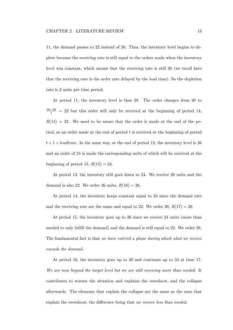
vided insight in the behavior of supply chains. Dejonckheere et al. [16] developed
ways to measure the bullwhip effect with control theory standard techniques. The
block diagram they used is the one presented in figure 2.2.
The two supply chain outputs which are modeled are the net stock-which cor-
responds to the inventory on hand, and the work in process-which is the number
of products already ordered in the past but not yet received. Looking at this block
diagram, we can note that the ordering policy is of the following form:
Ot = (Tp + 2) ∗ Dt − (NSt +WIPt),
where Dt is the forecasted demand for period t. The forecasting technique used
is an exponential smoothing. Tp represents the lead time. NS(t) and WIP (t) are
respectively the net stock and the work in process at period t. Along the thesis, for

CHAPTER 2. LITERATURE REVIEW 23
Figure 2.2: Block Diagram
any variable X, we use the two equivalent notations X(t) and Xt with no difference.
This ordering policy is an order-up-to level policy, in the sense that the ordering
level is determined by the difference between the forecasted demand over Tp + 2
periods and the inventory position, which is the number of products already ordered
(both on hand and in process). It is important to notice that, by definition, the
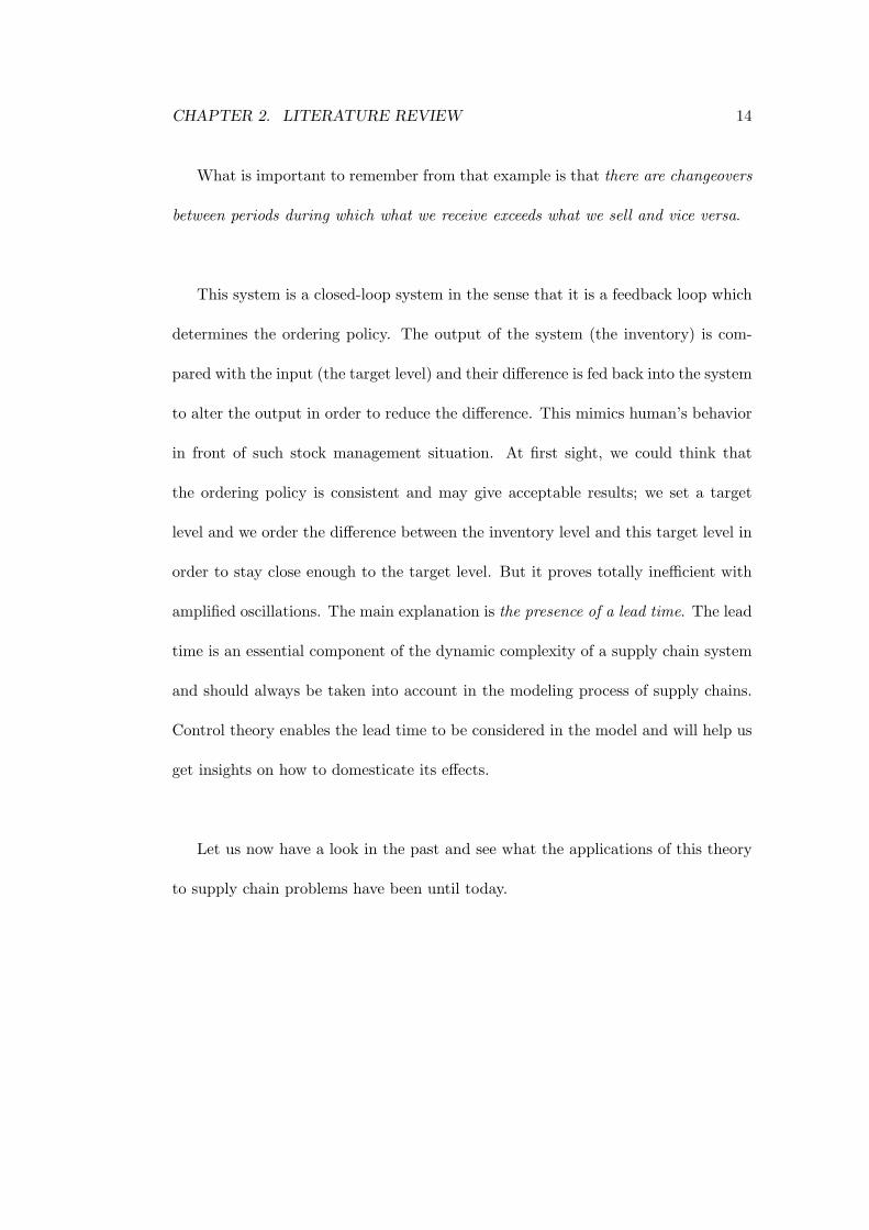
order Ot is made at the end of the period t. Thus, the corresponding products will
be received at the beginning of the period t+ Tp + 1. The figure below exhibits this
timeline:
In a more general perspective, the ordering policy is defined by:
Ot = (Tp + 1) ∗ Dt − (NSt +WIPt) + SSt,
where SSt represents a safety stock to prevent against uncertainty and changes. The
above model includes this safety consideration adding one period to the lead time,
which explains the form of the ordering policy. In the literature, we usually find

CHAPTER 2. LITERATURE REVIEW 24
Figure 2.3: Timeframe
safety stocks proportional to the variance of demand.
Using the frequency response plot, they were able to determine new bullwhip
effect metrics and study the impact of the exponential smoothing parameter for ex-
ample. One of their interesting results is the proof that such a replenishment rule
always results in some bullwhip effect: whatever the demand pattern is, the ratio of
the variance of orders over the variance of demand is greater than one. They stud-
ied other forecasting techniques and also proposed a replenishment rule generating
smooth ordering patterns with bullwhip effect ratios possibly less than one. The
fundamental idea of this replenishment rule is the use of proportional controllers of
the net stock and the work in process inventory. The replenishment rule they defined
actually is a generalisation of the ordering policy defined above. They used the term
‘fractional adjustments’ to actually describe the proportional controller technique.
We have already been through an explanation for such a controller: we want to fill
the gap between a defined target level and the current level at a rate which enables
to absorb the variations better.

CHAPTER 2. LITERATURE REVIEW 25
We will use the same kind of model for our system. The reasons for this choice
have already been highlighted: understanding the system from a dynamic point of
view, having a model which reproduces the stock manager perception of the system,
getting analytic results thanks to the use of control theory. Before getting to the
thick of things, let us introduce the systems dynamics methodology and its relevancy
to our study.
2.3 Systems dynamics and supply chains
In the early 60’s, Forrester [17], who was inducted into the Operational Research
Hall of Fame in 2006, introduced a new methodology the aim of which was to better
understand the dynamics of a system. This methodology is referred to as ‘System
Dynamics’ and is now applied to a wide number of systems. The fundamental of
this theory is the same as the grounds of Control Theory: feedback is the core tool
of the modeling process. The difference lies in the fact that System Dynamics is
more keen on using simulation whereas Control Theory tries to stay as much ana-
lytical as possible. The explanation is that the complexity of some systems makes
it very difficult to find analytical results. To do so, it usually requires numerous
simplifying assumptions. If we want to model the real complexity of the system, it
still is possible but the results will come from simulation. The combination of these
two techniques can provide great results in the sense that Control Theory brings
the necessary theoretical basis needed to analyze a system and System Dynamics
provides a framework for efficient simulation.
Another seemingly difference is that the systems dynamics methodology high-
lights the use of stocks and flows in the modeling process. It rather is a semantic

CHAPTER 2. LITERATURE REVIEW 26
difference in the sense that control theory just does not state it the same way, but
is more keen on using a rigorous mathematical tool which is differential equations.
Indeed, a flow is no more than the derivative of a stock. During the systems dynam-
ics conference this summer 2006, some people were confused about defining systems
dynamics as a field in itself, or as just a methodology, even if the question has al-
ready been answered some time ago by Ansoff and Slevin [18]. I tend to think that
it is rather a methodology. Its roots definitely belong to the control theory field.
Nevertheless, it is a wonderful methodology for modeling and simulating complex
systems, and the concepts and semantics which support the methodology are very
powerful, as for example the concept of stocks and flows which does not appear as
such in control theory. In my opinion, this concept would enhance students’ control
theory comprehension by making it more intuitive and less purely quantitative.
Sterman [6] wrote an exhaustive book treating the ‘System Dynamics’ theory
applied to business, economic and social systems. Four chapters of this book deal
with supply chain systems and an explanation of the oscillations that appear in sup-
ply chains is given. Our first example showed amplifying oscillations and we tried
to give an explanation for them. The lead time was the parameter which was at the
root of this problem. Sterman explains that “oscillation arises from the combination
of time delays in negative feedbacks and failure of the decision maker to take the
time delays into account.”
Supply chains may be the systems in which the concepts of time delays, stocks
and flows are the more blatant. Studying these systems from that perspective is
then very relevant to the understanding of these concepts. We would also like the
reader to keep in mind that our model can be applied to non-supply chain systems.

CHAPTER 2. LITERATURE REVIEW 27
For any model, as long as the concepts of stocks, flows and time delays appear in
the same fashion, the same dynamics will emerge.
Chapter 3
Description of the model
In this section, we describe our model of a single-stage single-product supply chain
with a periodic review. First, we define the ordering policy model which we will
study later on. Basically, it is a linear model with a non-linearity caused by the
possibility of shortages. Next, we will see that this model is a tool in itself to carry
out simulations, some of which will be presented. At the end, we introduce the profit
issue.
The final model we come up with is very similar to the one defined by Dejonck-
heere et al. [16]. The differences lie in the initialisation of the system, the possibility
of shortages and the introduction of the profit issue.
3.1 The ordering policy model
3.1.1 The basic model
As we said in the literature review, we will use control theory to develop our model,
extensively using the feedback concept. As described by Grubbstrom and Wikner
in [19], a basic production-inventory model can be described as in figure 3.1.
28

CHAPTER 3. DESCRIPTION OF THE MODEL 29
Figure 3.1: Basic production-inventory model
Let us describe this model.
The three fundamental information flows are the demand, the physical inventory
level or net stock, and the work-in-process. The net stock and the work-in-process
are considered to be feedbacks because they represent information which is fed back
into the system, in order to determine the quantity to order, which affects them in
return. The demand is considered to be a feedforward because it comes from the
outside of the system and the system structure does not affect the demand. In other
words, the implemented ordering policy only affects the feedbacks which are the net
stock and the work-in-process, not the feedforward which is the demand in our case.
Depending on the supply chain at hand, we have a total, partial or null influence
on the modules defined in the boxes. For instance and according to this model, we
can say that it is impossible to affect the demand which explains the absence of
input arrows into this module. On the contrary, we normally have a total control

CHAPTER 3. DESCRIPTION OF THE MODEL 30
on the ‘Demand Forecast’ and ‘Ordering Policy’ modules. This implies that it is up
to the decision makers to design effective policies to manage the system.
The ‘Demand Forecast’ and ‘Ordering Policy’ modules are black boxes in the
sense that everything can be done to determine the outputs of these boxes which
are the forecasted demand and the order rate respectively. This means that the out-
puts are mathematically determined by the inputs and any mathematical function
can be used in theory.
Along with the demand and the net stock which have obvious meanings, we have
introduced a very important variable for supply chains: the Work-In-Process inven-
tory denoted as WIP from time to time. We recall that it is the part of the inventory
which has been ordered but is not available yet to serve the demand. This variable
is the consequence of the lead time which is inherent to supply chains due to produc-
tion and/or distribution delays. It plays a key role because it determines how the
system can serve the demand in the coming periods. The WIP is the consequence
of the orders made in the past. If these past orders prove to be too high to serve the
actual demand, then the inventory will be greater than wanted, which is detrimental
since greater-than-expected holding costs will be incurred. On the contrary, if not
enough has been ordered, we might not have buffered enough against uncertainties.
As a consequence of a higher-than-expected demand, the demand may not be en-
tirely served and penalty costs may be incurred as well as a loss of sales.
An important issue is the demand forecasting in order to match the supply and
the demand. In the model, it is represented by the ‘Demand Forecast’ module.
We decide to forecast the one step ahead demand with the exponential smoothing

CHAPTER 3. DESCRIPTION OF THE MODEL 31
technique. This forecasting technique is easily understandable for managers and
widely used in the industry, which mainly explains our choice. Moreover, it is not
that obvious that more complicated techniques outperform this technique. It is very
popular to produce a smoothed time series. It consists of a weighted average of the
past observations, and it assigns exponentially decreasing weights as the observation
gets older. The exponential smoothing technique makes appear a single parameter
α and it is defined for a discrete signal as follows:
D(k) = α ∗D(k − 1) + (1− α) ∗ D(k − 1)
= α ∗ (D(k − 1) + (1− α) ∗D(k − 2) + (1− α)2 ∗D(k − 3) + ...)
where D(k) is the estimated value of the demand for period k and which is made
after we know the realised demand D(k − 1) at period k − 1.
The average age of the data is equal to (1−α)/α and is denoted Ta. It corresponds
to the amount of time by which forecasts tend to lag behind turning points in the
data. When making the forecast for period k, we know the demand until the period
k− 1. Then, if we are at period k− 1 making the forecast for period k, the average
age of the data is equal to:
Ta =∞∑n=0
weight ∗ age
=∞∑n=0
α ∗ (1− α)n ∗ n
=1− αα
.
It is judicious to notice that, in our calculation, the newest data is 0-period old.
From this relationship, we get the two reciprocal relations that we will use later on:
Ta =1− αα
α =1
1 + Ta.
Now that we have a forecast of the demand, we can define an ordering policy.
Periodically, we observe some pieces of information and decide on how much to order

CHAPTER 3. DESCRIPTION OF THE MODEL 32
for the next period. This is a feedback process. The information a stock manager
decides to observe is typically the net stock, the WIP and the forecasted demand.
Let us introduce or recall the useful variables of our system:
• NSt the inventory on hand (or net stock) at the end of period t
• WIPt the work-in-process at the end of period t
• InvPost the sum of the net stock and the work-in-process at the end of period
t, which is called the inventory position
• Ot the number of units ordered at the end of period t for serving the demand
of the next periods
• Dt the demand during period t
• Dt+1 the forecasted demand for period t+1 based on the observationsDt, Dt−1, ...
• Rt the number of units received at the beginning of period t
• LT the lead time
Another formalism can be found in the literature which does not differentiate
the beginning and the end of the periods. This formalism introduces a sequence of
events which would be in our case:
• first, we receive an order
• then, we serve the demand
• then, we update our NS and WIP values
• to conclude, we set a new order

CHAPTER 3. DESCRIPTION OF THE MODEL 33
It appears to us that differentiating the beginning and the end of the periods make
this sequencing more obvious and in a sense more rigorous, which explains why we
will stick to this first formalism. The figure 3.2 is presented in order to make the
different variables appear along the timeline.
Figure 3.2: The different variables along the timeline
The inventory on hand at the end of period t is the inventory on hand at the
end of the previous period plus the number of units received at the beginning of the
period minus the demand during this period:
NSt = NSt−1 +Rt −Dt. (3.1)
In the same way, we derive the relationship for the work-in-process. The WIP
at the end of period t is the sum of the WIP at period t − 1 plus the number of
units ordered at the end of the period minus the number of units received at the
beginning of period t:
WIPt = WIPt−1 +Ot−1 −Rt. (3.2)
When an order is placed at the end of period t, it takes some time for the products
to arrive in the inventory (production and distribution delay). As the order is placed

CHAPTER 3. DESCRIPTION OF THE MODEL 34
at the end of the period, it is as if it were made at the beginning of the next period.
So, the time delay between the orders variable index and the receiving variable index
is actually LT + 1 which includes one review period. It may appear more clearly in
figure 3.2. We thus have the relationship which can be easily checked for LT = 0:
Rt = Ot−LT−1 Ot = Rt+LT+1.
Let us now define what the ordering policy consists of.
Definition of the ordering policy
We will assume the ordering policy to be an order-up-to level policy. This means
that periodically, we set up a target level and we order the difference between this
target level and the actual level of our inventory position, which is defined over
the next LT+1 periods. Every period, the new observations allow to update the
target level according to the policy we choose. Usually, this target level is defined
as follows:
St = DLTt + SSt, (3.3)
where DLTt is an estimation of the expected demand over the lead time and SSt
is a safety stock for the period t. In the literature, we find many references to the
definition of the safety stock as the product of a safety factor k and the expected
variance of the demand over the lead time σ2LT . To simplify the model, setting the
safety factor to 0 and increasing the lead time by 1 has also been used.
We will use a third definition for our model which is more general in a sense. The
target level will consist of the sum of the expected demand over the lead time (to
fulfill the orders over the lead time-it is called the inventory position) plus a varying
term corresponding to the safety stock, which, if we wish, can be proportional to

CHAPTER 3. DESCRIPTION OF THE MODEL 35
the expected standard deviation over the lead time. Our model enables to define
the safety stock arbitrarily (which is interesting when thinking about simulations),
but most of the time, we will set this variable as constant in a simplification concern
during the analysis. Then, the number of units to order is defined as the difference
between a target level defined by the implemented policy and the current level.
Without additional information about the demand, our model assumes that the
expected demand over the lead time is calculated from the latest available value of
the expected demand. It is assumed to be equal to the expected value of the demand
times the number of periods of lead time:
DLTt = (LT + 1) ∗ Dt. (3.4)
Consequently, it follows an exponential smoothing pattern since we remind that the
forecasted demand follows such a pattern. So its behaviour is controlled by the
exponential smoothing parameter α.
The next relationship determines the order quantity:
O(t) = (LT + 1) ∗ Dt + SSt − InvPost
= LT ∗ D(t) + D(t) + SSt −WIPt −NSt
= (LT ∗ D(t)−WIP (t)) + D(t) + (SSt −NS(t)).
(3.5)
In order to improve this policy, we introduce TNS and TWIP as proportional
controllers on the Net Stock and WIP variables respectively. This is a very important
idea for this model. Using this type of controllers is second nature to experts in
control theory and we recall that Dejonckheere et al. [16] used this type of control
in their model. This means that after setting target values for these two variables, we
multiply the difference between the target value and the current value by a constant.

CHAPTER 3. DESCRIPTION OF THE MODEL 36
We can denote that if the constant is equal to one, it is equivalent to exactly order
this difference. Doing so can increase the performance of the system since we will
see that it provides a way for absorbing the variations of demand. The new order
quantity becomes:
O(t) =1
TWIP(LT ∗ D(t)−WIP (t)) + D(t) +
1TNS
(SSt −NS(t)). (3.6)
Figure 3.3 shows how this ordering policy is implemented with Matlab (as we
mentioned, the safety stock is defined as a constant here).
Figure 3.3: Ordering Policy
We can see different blocks with inputs and outputs the meanings of which vary:
• a triangle is the multiplication by a constant. The names of the correspond-
ing blocks are ‘Covering Time’, ‘WIP Adjusting Time’, ‘Net Stock Adjusting
Time’, ‘GainWIP’.
• transfer functions are defined by a rectangle in which the transfer function
appears. Since the signals are discrete signals, the Z-transform is used. The
CHAPTER 3. DESCRIPTION OF THE MODEL 37
understanding of the use of this transformation is not fundamental at the
moment and will be explained in the next chapter. These different blocks are
‘Exponential Smoothing’, ‘Review Period’, ’WIP Integration’, ‘Lag2’.
• we have also defined a function with three inputs and two outputs: ‘Net Stock
Integration’. The two ouputs defined at time t are the net stock at the end of
the period and the satisfied demand for this period. The three inputs are the
net stock at time t−1, the demand at time t and the number of units received
at the beginning of the period.
3.1.2 Comparison with the traditional base-stock policy
The traditional base-stock policy model is defined as follows: it is a periodic-review,
order-up-to-level policy where the review period is 1. At every period, an order is
made up to a certain level, but no order point is considered. The level is commonly
determined through the minimisation of a cost function comprising holding and
penalty costs. It is then almost the same policy as ours, except that the order-up-
to-level is fixed.
3.1.3 Introduction of the possibility of shortages
Shortages may happen when the demand exceeds the orders. It makes non-linearities
appear in the system. Non-linearities are more difficult to analyse, but they can
be modeled easily. Nonlinearity arises in the definition of the function ‘Net Stock
Integration’ since the function is defined as follows:
if Dt < Rt +NSt−1,
then NSt = NSt−1 +Rt −Dt and SatisDt = Dt;
else NSt = 0 and SatisDt = NSt−1 +Rt,

CHAPTER 3. DESCRIPTION OF THE MODEL 38
where SatisDt is the satisfied (or served) demand for the period t.
This also requires to add a new variable UnSatisDt which is the number of
unsatisfied orders at period t which are going to be served as soon as possible. It is
defined by:
UnSatisDt = D∗t − SatisDt, (3.7)
with the new demand D∗t being:
D∗t = Dt + UnSatisDt−1. (3.8)
If we want to take the backlog into account in the model, we need to add an
unsatisfied demand variable, with a one period lag, which buffers the unsatisfied
orders. The realised demand of a period is then equal to the sum of this unsatisfied
demand and the usual demand.
3.1.4 Initialisation
We have also added some boxes in order to initialise the system. They do not appear
in the diagram but will appear later. The values which need this initialisation are
the net stock, the work in process, the orders of the first periods. This question
of the initialisation is not theoretically fundamental but necessary in order to get
correct simulation results.
The initial value of the net stock should be close enough to the initial target net
stock.
The initial value of the work in process should also be close enough to the initial
target value. The work in process target value is defined as the forecasted demand
multiplied by the lead time. We use our knowledge on the demand to define the
initial value. For instance, if we decide to model the demand as a gaussian process

CHAPTER 3. DESCRIPTION OF THE MODEL 39
with a mean µ, we initialise the work in process with the value:
WIP = µ ∗ LT.
In the same way, the first receipts should serve the first demands until the first
order really made arrives. The first order made at the end of period 1 will arrive at
the beginning of period LT + 1. So we define the receipts for the periods 1,...,LT.
Since we are able to define the demand independently, we have access to it before
simulating the system. The choice that we made is that the initial receipts are all the
same and equal to the calculated mean of demand over this lead time LT . Thanks
to this, the initial orders correspond to the initial demands in a satisfactory way.
3.1.5 Final model
Thus, we get the following model (figure 3.4). This model is an achievement in
itself and can be used to carry out simulations. It enables to build intuition about
the behavior of our system. We have indicated with colored boxes the main parts:
the net stock and work in process calculation in red, the ordering policy including
the forecast in blue, the two inputs in orange, the four outputs in green. Even if
analysis provides a way for a theoretical understanding of the system, it can prove
very difficult to get results. Then simulations become the best way to understand
the system, even if it is not as rigorous as analysis. They also prove useful to visualise
how the system behaves under particular conditions, like the conditions of shortages,
which are very difficult to analyse. As explained in the introduction, we will present
an analysis of the system in chapter 5.

CHAPTER 3. DESCRIPTION OF THE MODEL 40
Figure 3.4: Final Ordering Policy Model

CHAPTER 3. DESCRIPTION OF THE MODEL 41
3.2 Simulations
Now, we are able to present the results of some simulations. The prime aim of our
study is not to present simulations, so we just present two simulations in order to
make the reader more familiar with the system. However, we would like to highlight
the fact that simulation helps build intuition about the system, and we personally
used it as such. These simulations were carried out with the following parameters:
• LT = 10,
• TNS = TWIP = 4,
• Demand D ∼ N(100, 5) normal distribution with mean 100 and variance 5,
• α = 0.2.
The two simulations differ by the safety stock level which has some incidence.
For the first simulation, we define a safety stock such that there is no shortage (the
probability of having a shortage is theoretically not zero but very weak). For the
second simulation, the safety stock is lower and it results in a shortage.
The figures 3.5 and 3.6 show the net stock, the orders, the work in process and
the demand for the first simulation. The results for the second simulation are shown
in figures 3.7 and 3.8.
The system we have defined enables for various simulations. We can define dif-
ferent demand patterns, assign different values to the ordering policy parameters
(exponential smoothing parameter, adjusting parameters) and determine the target
safety stock over the simulation time length.

CHAPTER 3. DESCRIPTION OF THE MODEL 42
Figure 3.5: Simulation 1: the Demand (no shortage)
Figure 3.6: Simulation 1: NS, WIP and Orders (no shortage)

CHAPTER 3. DESCRIPTION OF THE MODEL 43
Figure 3.7: Simulation 2: the Demand (two shortages)
Figure 3.8: Simulation 2: NS, WIP and Orders (two shortages)

CHAPTER 3. DESCRIPTION OF THE MODEL 44
First simulation
The first simulation shows a quite stable system in the sense that the variables
evolve around their mean values. Some remarks can be done. For instance, we can
notice that the net stock and work-in-process do not seem to be i.i.d variables as the
demand is. It also seems to be some correlation between these two variables with
higher values of one corresponding to lower values of the other. Even if we will not
explore this way of study, it shows how valuable simulation can be when it comes
to build intuition on complex systems.
Second simulation
The second simulation exhibits a shortage around time 40 with backordering, the
unsatisfied orders are kept in memory and served in the next periods. This shortage
is due to the low level of the safety stock. By observing the net stock, we see that a
big overshoot follows this shortage. We easily figure out how detrimental it is since
this extra inventory will incur unnecessary high holding costs. The system with
non-linearity is difficult to analyse but it is still possible to draw conclusions with
such simulations.
Simulation is very useful with regards to two situations:
• when we want to build some intuition,
• when the system is too complex to analyse.
Our model and its implementation in Matlab is consequently a useful tool to the
understanding of ordering systems.

CHAPTER 3. DESCRIPTION OF THE MODEL 45
3.3 Introduction of the profit into the model
As we stated before, we want to define a profit function to control the supply chain
performance. Consequently, we introduce these variables into the model. We are
going to consider the holding costs, the purchasing costs and the sales. The holding
costs correspond to what the company pays to store the products. The purchasing
costs are paid at the receipt of the product or the material before transformation.
This is not an assumption with no consequences. We could have assumed that the
payment be made when the order is made or whatsoever. In the long run, it does
not affect the system’s performance since it corresponds to a translation of time but
it may have a short term impact.
Let us now introduce some notations:
• h is the holding unit cost;
• Psale is the selling unit price;
• Ppur is the purchasing unit price.
In the case of a fully satisfied demand, the cash flow for the period t is defined
by:
CashF lowt = Psale ∗Dt − Ppur ∗Rt − h ∗NSt (3.9)
It becomes more complicated if a shortage occurs because the demand would
depend on the past unsatisfied orders. But the relationship is the same except that
only the satisfied demand is taken into account to calculate the cash flow:
CashF lowt = Psale ∗ SatisDt − Ppur ∗Rt − h ∗NSt (3.10)

CHAPTER 3. DESCRIPTION OF THE MODEL 46
We introduce the necessary boxes into the simulation model which gives the final
model of our ordering policy in figure 3.9. This model can then be used to simulate
different types of situations and proves to be a very useful tool.
Figure 3.9: The ordering policy model
The profit functions of the previous simulations are presented in figures 3.10
and 3.11. First of all, we notice that the mean cash flows are greater in the second
simulation than in the first one. Since the target safety stock is greater in simulation
1, then its holding costs are bigger whereas the sales and purchasing costs do not
change (the demand remaining the same). As long as there is no shortage, the lesser
the target safety stock, the better. But what happens when a shortage occurs?
As expected, the simulation 2 cash flow figure exhibits one huge decrease which
corresponds to the aftermath of the shortage which happens around the time 55. It
is a consequence of the excessive net stock which reaches very high values. There
are different phenomena explaining this situation. First, when the system safety
stock is below the target value, then it starts ordering more to bridge the gap.
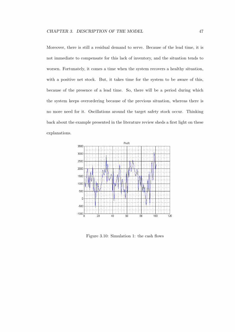
CHAPTER 3. DESCRIPTION OF THE MODEL 47
Moreover, there is still a residual demand to serve. Because of the lead time, it is
not immediate to compensate for this lack of inventory, and the situation tends to
worsen. Fortunately, it comes a time when the system recovers a healthy situation,
with a positive net stock. But, it takes time for the system to be aware of this,
because of the presence of a lead time. So, there will be a period during which
the system keeps overordering because of the previous situation, whereas there is
no more need for it. Oscillations around the target safety stock occur. Thinking
back about the example presented in the literature review sheds a first light on these
explanations.
Figure 3.10: Simulation 1: the cash flows

CHAPTER 3. DESCRIPTION OF THE MODEL 48
Figure 3.11: Simulation 2: the cash flows (shortage)

Chapter 4
Control theory tools
The aim of this chapter is to make the reader more familiar with the control theory
tools that we are about to use to analyse the system. It is a very brief introduction
and has the practical purpose to make the reader understand what will follow. The
reader should refer to appropriate books to go further (see for example [4], [20], [21]).
For each point, we give the reason why we need it even though it will be clearer
along the analysis.
Even if we highlighted a nonlinearity in the system, we will focus on the linear
part of the system during the analysis. What is presented hereafter is then only
relative to linear systems.
4.1 A fundamental result on linear systems
Let us consider a linear system, meaning that the relationships between the variables
are linear, with a single input and a single output. One fundamental result for such
a system is that if the input is a sine function with amplitude A and frequency f ,
A ∗ cos(2π ∗ ft), then the output is also a sine function with the same frequency,
49

CHAPTER 4. CONTROL THEORY TOOLS 50
B ∗ cos(2π ∗ ft+ φ), the amplitude B and the phase φ having possibly changed.
Provided this result, one of the tools that we will use is the amplitude Bode
diagram. For a single-input single-output system, such a diagram represents the
ratio of the amplitude of the output over the amplitude of the input for different
frequencies, assuming the input to be a sine wave. Then, this diagram shows how a
sine wave is transformed by our system in terms of amplitude.
4.2 The z-transform
This transformation is a discrete version of the Laplace transform which is used for
continuous systems. It transforms a discrete time function into a complex function:
RN −→ CC
k 7→ f(k) 7−→ z 7→ F (z) =∞∑
k=−∞f(k)z−k.
Our ordering policy system exhibits discrete time functions (or relationships
between variables). One of the fundamental ideas in control theory is to transpose
the problem into the frequency domain using the z-transform, and then to use the
nice properties of the z-transform to get results. Difficult problems in the time
domain can become easy in the frequency domain, and vice versa. We will apply
this transformation to the relationships between the variables of our system.
The important properties that we will use are the linearity of this transformation
and the advance (and delay) property which allows the calculation of the z-transform
of a discrete function which has been shifted n samples to the left (to the right).
The advance (delay) property states that if the z-transform of the original function
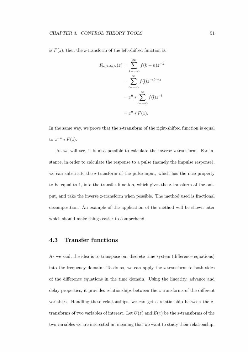
CHAPTER 4. CONTROL THEORY TOOLS 51
is F (z), then the z-transform of the left-shifted function is:
Fleftshift(z) =∞∑
k=−∞f(k + n)z−k
=∞∑
l=−∞f(l)z−(l−n)
= zn ∗∞∑
l=−∞f(l)z−l
= zn ∗ F (z).
In the same way, we prove that the z-transform of the right-shifted function is equal
to z−n ∗ F (z).
As we will see, it is also possible to calculate the inverse z-transform. For in-
stance, in order to calculate the response to a pulse (namely the impulse response),
we can substitute the z-transform of the pulse input, which has the nice property
to be equal to 1, into the transfer function, which gives the z-transform of the out-
put, and take the inverse z-transform when possible. The method used is fractional
decomposition. An example of the application of the method will be shown later
which should make things easier to comprehend.
4.3 Transfer functions
As we said, the idea is to transpose our discrete time system (difference equations)
into the frequency domain. To do so, we can apply the z-transform to both sides
of the difference equations in the time domain. Using the linearity, advance and
delay properties, it provides relationships between the z-transforms of the different
variables. Handling these relationships, we can get a relationship between the z-
transforms of two variables of interest. Let U(z) and E(z) be the z-transforms of the
two variables we are interested in, meaning that we want to study their relationship.

CHAPTER 4. CONTROL THEORY TOOLS 52
Then the transfer function of U(z) relative to E(z) can be written:
U(z)E(z)
=a0 + a1 ∗ z−1 + ...+ ap ∗ z−p
b0 + b1 ∗ z−1 + ...+ bq ∗ z−q,
with (a0, ..., ap) ∈ Rp, (b0, ..., bq) ∈ Rq, (p, q) ∈ N2.
An important remark is that we reason by difference to an equilibrium state.
So when we apply the z-transform to the equations, the constant terms relative to
this equilibrium state disappear. The reader should keep this in mind since this will
apply to the calculus of the next chapter.
4.4 Stability
There exist many concepts of stability in control theory. Stability is the property
of an equilibrium state. For proper operation of any system, stability is the main
requirement. When stability is ensured, then other requirements can be obtained
such as dynamic performance. The study of the stability of non-linear systems is
much more complex than for linear systems. One main difference is that linear sys-
tems only have one equilibrium state.
The stability is important with regards to our problem. The ordering policy
should be as much stable as possible in order to react in a decent way to variations
in the system. Control theory provides a theoretical framework to understand this
concept from a quantitative point of view.
The concept of stability that we will use is called Bounded Input/Bounded Out-
put stability, which we can refer to as BIBO. That means that for any bounded
input, the output of the system is bounded. When it will come to study the stabil-
ity of the system, we will use the result that it is equivalent for the corresponding
transfer function (as a rational of the variable z) to have all its poles inside the unit

CHAPTER 4. CONTROL THEORY TOOLS 53
circle. It is also equivalent to the definite absolute sum of the impulse response. Let
h be the impulse response (which is the output of the system when the input is a
pulse). Then, a system is BIBO stable if and only if:
∞∑n=0
|h(n)| <∞.
There is another type of stability which is called asymptotic stability and which
corresponds to the convergence to zero of the impulse response (the system gets
back to its initial state). The condition for asymptotic stability is that the transfer
function has its poles strictly inside the unit circle. It is then easy to see that the
asymptotic stability implies the BIBO stability.
4.5 The Tsypkin Theorem
One definition for the bullwhip effect is the ratio of the variance of the orders over
the variance of the demand. There exists a theorem proved by Tsypkin [22] which
allows for such a calculation with the particular assumption of the input being an
independent and identically distributed random variable. This theorem states that
the variance of a system’s output divided by the variance of the system’s input is
equal to the sum of the squared impulse response. Let f be the impulse response,
σ2input and σ2
output respectively the variances of the input and output variables. Then,
the theorem is:∞∑k=0
f(k)2 =σ2output
σ2input
.
This theorem will then be used to calculate the bullwhip effect metric when the
system faces an independent and identically distributed demand.
Chapter 5
Analysis of the ordering policy
Let us analyse the system we have defined thanks to control theory tools. The aim
is to understand its dynamical properties and to work out managerial insights: we
are mainly interested in the bullwhip effect and the flexibility.
In a first step, we determine the transfer functions of the variables of interest
which are the orders, the net stock and the work-in-process. Then, we derive the
Bode diagrams of these variables, study the influence of the parameters and draw
conclusions regarding the bullwhip effect. After that, we take another approach to-
wards the bullwhip effect and derive formula to calculate it within some assumptions
frame.
The second step focuses more on the time aspect, with the use of step responses.
The goal is the same, working out managerial insights regarding the bullwhip effect
and the flexibility issues. After that, we highlight the tradeoff which appears be-
tween having a weak bullwhip effect and being flexible. Then, the effect of the lead
time is studied and we finish with an analysis of the profit issue for this system.
54
CHAPTER 5. ANALYSIS OF THE ORDERING POLICY 55
5.1 Transfer functions of the ordering policy
5.1.1 Deriving the order, work-in-process and net stock transfer
functions
In a first step, let us determine the transfer function of the system with the point of
view of the input being the demand and the output being the orders. Let us recall
that we only consider linear systems, which for our system means that we do not
take the possibility of shortage into account. We will make the difference between
the functions of discrete time from the functions of frequency denoting the former
fk or f(k) and the latter fz or f(z) for a particular function f . k and z denote
discrete time and complex variables respectively.
The time relationship:
D(k) = α ∗D(k) + (1− α) ∗ D(k − 1),
becomes in the frequency domain:
D(z)D(z)
=α
1− (1− α)z−1,
which we can also write using the parameter Ta = 1−αα :
D(z)D(z)
=1
(1 + Ta)− Taz−1.
The three relationships for the WIP, the Net Stock, and the Received Orders
are:
WIPk = WIPk−1 +Ok−1 −Rk
NSk = NSk−1 +Rk −Dk
Rk = Ok−LT−1,

CHAPTER 5. ANALYSIS OF THE ORDERING POLICY 56
which turns in the frequency domain into:
WIP (z) = z−1 ∗WIP (z) + z−1 ∗O(z)−R(z)
NS(z) = z−1 ∗NS(z) +R(z)−D(z)
R(z) = z−LT−1 ∗O(z).
The next relationship determines the order quantity in the time domain:
O(k) = D(k) +1
TWIP(LT ∗ D(k)−WIP (k)) +
1TNS
(SS −NS(k)).
We assume the safety stock to be constant as stated in the description of the model.
This relationship turns in the frequency domain into:
O(z) = D(z) +1
TWIP(LT ∗ D(z)− 1
1− z−1∗ (z−1O(z)−R(z)))
− 1TNS
∗ 11− z−1
(R(z)−D(z))
=1
1 + Ta − Taz−1∗ (1 +
LT
TWIP)D(z)− 1
TWIP (1− z−1)(z−1O(z)−R(z))
− 1TNS(1− z−1)
(R(z)−D(z))
=[ 1
1 + Ta − Taz−1∗ (1 +
LT
TWIP) +
1TNS(1− z−1)
]D(z)
− 11− z−1
(1
TWIP(z−1 − z−LT−1) +
1TNS
z−LT−1)O(z),
which simplifies after some calculation to:
O(z)D(z)
=(TWIP + LT + TWIP
TNS(1 + Ta))− z−1(TWIP + LT + TWIP
TNSTa)
(1 + Ta − Taz−1)(TWIP + z−1(1− TWIP ) + z−LT−1(TWIPTNS
− 1)). (5.1)
The particular case where TWIP = TNS makes the transfer function more simple:
O(z)D(z)
=(TWIP + LT + 1 + Ta)− z−1(TWIP + LT + Ta)
(1 + Ta − Taz−1)(TWIP + z−1(1− TWIP )). (5.2)
In the same way that we have defined the relationship between the orders and the
demand, we can determine the relationship between any output and the demand. We

CHAPTER 5. ANALYSIS OF THE ORDERING POLICY 57
still consider a linear model. Let us begin with the net stock. The time relationship
for the net stock is:
NS(k) = NS(k − 1) +R(k)−D(k)
= NS(k − 1) +O(k − LT − 1)−D(k).
It gives the following transfer function relationship:
NS(z)(1− z−1) = z−LT−1O(z)−D(z)
= (z−LT−1∗(TWIP + LT + TWIP
TNS(1 + Ta))− z−1(TWIP + LT + TWIP
TNSTa)
(1 + Ta − Taz−1)(TWIP + z−1(1− TWIP ) + z−LT−1(TWIPTNS
− 1))−1)∗D(z).
(1− z−1) ∗ NS(z)D(z)
=−(1 + Ta)TWIP
(1 + Ta − Taz−1)(TWIP + z−1(1− TWIP ) + z−LT−1(TWIPTNS
− 1))
+ z−1 ∗ −TaTWIP + (1 + Ta)(1− TWIP )(1 + Ta − Taz−1)(TWIP + z−1(1− TWIP ) + z−LT−1(TWIP
TNS− 1))
+ z−2 ∗ Ta(1− TWIP )(1 + Ta − Taz−1)(TWIP + z−1(1− TWIP ) + z−LT−1(TWIP
TNS− 1))
+ z−LT−1 ∗ TWIP + LT + 1 + Ta
(1 + Ta − Taz−1)(TWIP + z−1(1− TWIP ) + z−LT−1(TWIPTNS
− 1))
+ z−LT−2 ∗ −(TWIP + LT + Ta)(1 + Ta − Taz−1)(TWIP + z−1(1− TWIP ) + z−LT−1(TWIP
TNS− 1))
.
Finally, the transfer function is:
NS(z)D(z)
=−(1 + Ta)TWIP + z−1(−TaTWIP + (1 + Ta)(1− TWIP )) + z−2(Ta(1− TWIP ))
(1− z−1)(1 + Ta − Taz−1)(TWIP + z−1(1− TWIP ) + z−LT−1(TWIPTNS
− 1))
+z−LT−1(TWIP + LT + 1 + Ta) + z−LT−2(−(TWIP + LT + Ta))
(1− z−1)(1 + Ta − Taz−1)(TWIP + z−1(1− TWIP ) + z−LT−1(TWIPTNS
− 1)).
(5.3)
From the work in process time relationship:
WIP (k) = WIP (k − 1) +O(k − 1)−R(k),
we conclude:
WIP (z)D(z)
=z−1 − z−LT−1
1− z−1∗
(TWIP + LT + TWIPTNS
(1 + Ta))− z−1(TWIP + LT + TWIPTNS
Ta)
(1 + Ta − Taz−1)(TWIP + z−1(1− TWIP ) + z−LT−1(TWIPTNS
− 1)).
(5.4)
CHAPTER 5. ANALYSIS OF THE ORDERING POLICY 58
5.1.2 Stability of the system
There exist different concepts of stability in control theory. The stability we will be
interested in is the one corresponding to convergence and/or non-divergence of the
variables of the system. We will study the Bounded Input/Bounded Output (BIBO)
and asymptotic stabilities that we have already presented in chapter 4. The results
for these two types of stability only differ by the fact that the inequalities on the
parameters TWIP and TNS are strict in the case of the asymptotic stability. The
aim is to determine the stability of the ordering policy we defined.
We recall that to study the stability of interest, we have to determine the poles
(the zeros of the denominator) of the transfer functions and see whether they lie
outside or inside the complex unit circle. These results have already been stated in
chapter 4. The aim is to determine conditions on the parameters TWIP and TNS
to obtain the required stability. We will not consider the three transfer functions of
order, net stock and work-in-process because they actually have the same poles. So
we will only study the order transfer function and the stability results for the net
stock and work-in-process variables will be the same. We will consider the transfer
functions as rationals in z−1 (as if the variable is z−1 instead of z), then the con-
dition for asymptotic stability is that the poles strictly lie outside the unit circle
(|z| < 1 is equivalent to |z−1| > 1). We also recall that the proportional controllers
are positive real numbers.
The poles of the order transfer function (as a rational in z−1) are 1+TaTa
and the
LT + 1 zeros of the polynomial TWIP + z−1(1− TWIP ) + z−LT−1(TWIPTNS
− 1)). Since
1+TaTa
> 1, there is no stability problem: this root is strictly outside the unit circle.

CHAPTER 5. ANALYSIS OF THE ORDERING POLICY 59
What about the polynomial? To determine the possibility of roots inside the
unit circle, we can assume the complex number z−1 to be in the unit circle, and see
the area described by the polynomial when the variable z−1 describes the unit circle
denoted Γ(0, 1). We denote Γ(z, r), with z a complex number and r a non-negative
real number, the area delimited by the circle of center z and radius r. The condition
is then given by the possibility of the complex number 0 to be in this area or not.
This can be seen as a graphical method in the complex plan. We recall that the
assumptions are TWIP , TNS > 0, LT ≥ 1.
Case 1: TWIP = 1
The polynomial becomes 1 + z−LT−1( 1TNS− 1)). Its roots strictly lie outside the
unit circle if and only if z−LT−1 ∗ (TNS − 1) < 1 that is, since z−LT−1 ∈ Γ(0, 1),
| 1TNS− 1| < 1 which gives 0.5 < TNS (the case TNS = 1 is obvious).
Case 2: TWIP > 1
We have TWIP + z−1(1− TWIP ) ∈ Γ(TWIP , TWIP − 1). Since z−LT−1(TWIPTNS
− 1) ∈
Γ(0, |TWIPTNS
− 1|), a sufficient condition for the roots to strictly lie outside the unit
circle is TWIPTNS−1 < 1, that is TWIP
TNS< 2. We can remark that it is the same condition
as for the case TWIP = 1.
Case 3: 0.5 < TWIP < 1
We have TWIP + z−1(1 − TWIP ) ∈ Γ(TWIP , 1 − TWIP ), whose minimum module
point is the real number 2 ∗ TWIP − 1. Since z−LT−1(TWIPTNS
− 1) ∈ Γ(0, |TWIPTNS
− 1|),
a sufficient condition is then 2 ∗ TWIP − 1 > |TWIPTNS
− 1|. This is equivalent to
1−2∗TWIP <TWIPTNS
−1 < 2∗TWIP −1, that is TNS > 0.5 and 2∗(1−TWIP ) < TWIPTNS
with 2 ∗ (1− TWIP ) < 1 in this case.
CHAPTER 5. ANALYSIS OF THE ORDERING POLICY 60
Case 4: TWIP ≤ 0.5
There can happen stability problems with roots lying inside the unit circle. In other
terms, 0 is inside the area describes by the polynomial when z describes the unit
circle Γ(0, 1).
Hence, to get a stable system, we should restrict our study to the case TWIP > 0.5
and the subsequent conditions for the different cases 1,2 and 3.
Interestingly, we notice that setting TWIP = TNS > 0.5 makes the system stable
according to the conditions stated above. It also makes the transfer function more
simple and will allow for more analytical results. This will be the second restriction
of our study even though our stability results hold for TWIP 6= TNS . There must
be interesting developments by studying the decoupling of the net stock and the
work in process adjusting parameters, but the analysis is more complex and is not
within the prime scope of our study. That is why we will focus on this particular case.
Let us now analyse the dynamics of the model under this new assumption frame-
work which we recall here:
TWIP = TNS > 0.5. (5.5)
The motivation for such a restriction is the stability of the system and a simplifica-
tion of the system which will allow for analytical results.
We want to understand how the stable system behaves in a dynamical environ-
ment, and to point out some properties of its dynamical behaviour.

CHAPTER 5. ANALYSIS OF THE ORDERING POLICY 61
5.2 A frequency approach to the bullwhip effect
5.2.1 Bode diagrams
We are about to study the dynamics of the model with a focus on the frequency
aspect. How does the system behave at a particular frequency? What about the
bullwhip effect?
Now that we have calculated the transfer functions, it is easy to get the Bode
diagrams. Since we are only considering in this part linear systems, we recall here
that if the input of the system is a sine wave, then the output is also a sine wave, the
very important thing being that it has the same frequency, but not necessarily the
same amplitude nor the same phase. A Bode diagram represents for each frequency,
the amplitude and the phase of such an output.
The meaning of the frequency is to be linked to the time period between two
orders, which is the unit of time of our system. Hence, a frequency of 0.1Hz is
equivalent to a period of time of 10.1 = 10 inter orders-arrival time equivalent. If the
time between two orders is ten days, then the period corresponding to the frequency
of 0.1Hz is 100 days.
In figure 5.1, we present the Bode diagram of the transfer function relative to
the orders O(z)D(z) , with the parameters LT = 10, TNS = TWIP = 5, α = 0.1.
We find that for the frequencies up to 0.085Hz (11.76 periods), the amplitude
is greater than one, meaning that there is an increase of amplitude of the sine wave
in input, or said in supply chain terms, a bullwhip effect. Indeed, an increase of
amplitude means a greater variation of the orders (the output) over the demand
(the input). But for the frequencies greater than 0.085Hz (11.76 periods), there is
no bullwhip effect and even a reduction of the amplitude. This is enabled by the

CHAPTER 5. ANALYSIS OF THE ORDERING POLICY 62
Figure 5.1: Bode diagram in amplitude relative to the orders
existence of the proportional controllers which are set to a greater value than one
in that case. Otherwise, with proportional controllers set to one, which means that
we exactly order the difference between the target level and the current level, we
get the diagram of figure 5.2 which shows that it is impossible to avoid the bull-
whip effect for sine waves since all the values for every frequency are greater than one.
The effect of the adjusting parameters (or proportional controllers) on the orders
transfer function can be seen on the figure 5.3 where the Bode diagrams are presented
for different values of these parameters varying from 1 to 10.
For the low frequencies sine waves, low adjusting parameters are better if we
want to get the smallest ordering amplitude possible. But this holds up to a certain
frequency, beyond which greater adjusting parameters perform better.
Depending on the demand pattern at hand, managers can take this approach to
try to dampen the bullwhip effect. For instance, it gives a way to understand how
the seasonality modeled as a sine wave affects the system in terms of bullwhip effect.
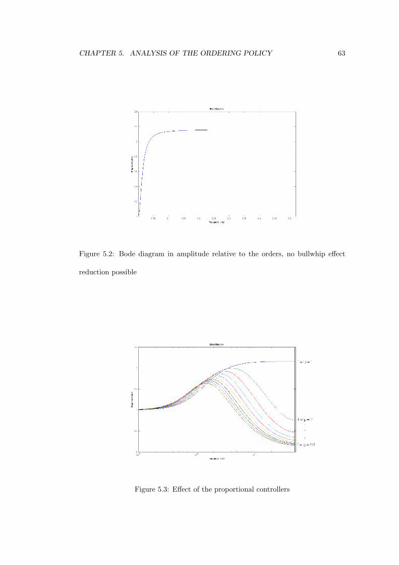
CHAPTER 5. ANALYSIS OF THE ORDERING POLICY 63
Figure 5.2: Bode diagram in amplitude relative to the orders, no bullwhip effect
reduction possible
Figure 5.3: Effect of the proportional controllers

CHAPTER 5. ANALYSIS OF THE ORDERING POLICY 64
To give a numerical example, for a particular set of parameters TWIP = TNS = 1,
α = 0.1, for a lead time equal to LT = 10 and a seasonality effect with a period
Tseason = 40 which corresponds to the sine wave period, then the contribution of
the ordering policy to the bullwhip effect, in other words the ratio of the variations
of the orders over the variations of the demand, is calculated by getting the Bode
diagram value at the frequency f = 1/40. It is equal to about 1.87.
We have simulated such a system with a view to better understanding this result,
and checking this analytical result. The results of the simulation with the same set
of parameters are presented in figure 5.4. We just show the demand (in red) and
the orders (in blue).
Figure 5.4: An example of seasonal bullwhip effect
The demand is a sine wave at the frequency f = 1/40 with a mean equal to 100,
and the amplitude of the variations equal to 1. As expected, the order is a sine wave
at the same frequency, its mean also is 100 and the amplitude of the variations is
equal to 1.87, as we could read on the Bode diagram.
We now take a different approach towards the bullwhip effect considering how

CHAPTER 5. ANALYSIS OF THE ORDERING POLICY 65
the system behaves facing an independent and identically distributed demand.
5.2.2 Independent and identically distributed demand
In a random variable context, the bullwhip effect is generally defined as the ratio of
the variance of orders over the variance of the demand. We will use a fundamental
result from Tsypkin, already presented in chapter 4, to calculate this metric. To
recall it, this result states that the variance of a system’s output divided by the
variance of the input is equal to the sum of the squared impulse response. There is
a restriction however: the input needs to be independent and identically distributed
(i.i.d.). It is sometimes possible to calculate analytically the impulse response
of a system by calculating the inverse z-transform of the transfer function. We
previously calculated this function which was under the assumption TWIP = TNS :
O(z)D(z)
=(TWIP + LT + 1 + Ta)− z−1(TWIP + LT + Ta)
(1 + Ta − Taz−1)(TWIP + z−1(1− TWIP )).
The general case
Let us rewrite it in a more simple form (fractional decomposition) so as to easily
calculate the inverse z-transform:
O(z)D(z)
=TWIP + LT + 1 + Ta
(1 + Ta)TWIP∗
1− TWIP +LT+Ta
TWIP +LT+1+Taz−1
(1− Ta1+Ta
z−1)(1− (1− 1TWIP
)z−1)
=A ∗ 1− α ∗ z−1
(1− β ∗ z−1)(1− γ ∗ z−1)
=A ∗ (n1
1− β ∗ z−1+
n2
1− γ ∗ z−1),

CHAPTER 5. ANALYSIS OF THE ORDERING POLICY 66
where:
A =TWIP + LT + 1 + Ta
(1 + Ta)TWIP
α =TWIP + LT + Ta
TWIP + LT + 1 + Ta
β =Ta
1 + Ta
γ =1− 1TWIP
,
and n1, n2 ∈ R such as:
n1 + n2 =1
n1 ∗ γ + n2 ∗ β =α,
that is:
n1 =α− βγ − β
=TWIP (LT + TWIP )
(LT + TWIP + Ta + 1)(TWIP − 1− Ta)
n2 =γ − αγ − β
=(1 + Ta + LT )(1 + Ta)
(LT + TWIP + Ta + 1)(1 + Ta − TWIP ).
It is important to notice that such a decomposition is correct under two assump-
tions. The first one is TWIP 6= 1. By continuity, we will assume that our final result
holds when TWIP = 1. The second assumption is α, β, γ all different - that is, after
simplification, 1 + Ta 6= TWIP (since α is always different from β and γ because
α = β is equivalent to TWIP +LT = 0 and α = γ is equivalent to LT + Ta + 1 = 0).
We study later what happens in the case 1 + Ta = TWIP .
We eventually get the z-inverse transform using the linearity and the fact that
the z-inverse transform of 11−a∗z−1 is an∗1(n) where 1 is the Heavyside echelon equal
to 1 for n ≥ 0, and 0 otherwise. Thus, we get the z-inverse transform of the transfer
function O(z)D(z) :
Z−1(O(z)D(z)
)(n) = f(n) =LT + TWIP
(1 + Ta)(TWIP − 1− Ta)∗(
Ta1 + Ta
)n∗ 1(n)
+1 + Ta + LT
TWIP (1 + Ta − TWIP )∗(
1− 1TWIP
)n∗ 1(n).

CHAPTER 5. ANALYSIS OF THE ORDERING POLICY 67
We would like to bring two remarks to the reader. The first one is that the
above function is actually the impulse response. We will use it to calculate some
bullwhip effect metric but it can be used to serve other purpose. The second one
is that the impulse response converges to zero if and only if |1 − 1TWIP
| < 1, that
is TWIP = TNS > 0.5. We fall again on the stability result. We recall that the
asymptotic stability means the convergence of the impulse response to zero.
Now we can calculate the ratio of the variance of the orders over the variance of
the demand when the demand is i.i.d. This ratio is equal to:
σ2Order
σ2Demand
=+∞∑n=0
f(n)2
= A2 ∗ (n2
1
1− ( Ta1+Ta
)2+
n22
1− (1− 1TWIP
)2+
2n1n2
1− Ta1+Ta
(1− 1TWIP
))
=( LT + TWIP
(1 + Ta)(1 + Ta − TWIP ))2 ∗ 1
1− ( Ta1+Ta
)2
+( 1 + Ta + LT
TWIP (1 + Ta − TWIP ))2 ∗ 1
1− (1− 1TWIP
)2
− 2(LT + TWIP )(1 + Ta + LT )
TWIP (1 + Ta)(1 + Ta − TWIP )2∗ 1
1− Ta1+Ta
(1− 1TWIP
).
(5.6)
This result enables for the calculation of the bullwhip effect implied by the
ordering policy when the demand is independent and identically distributed.
The particular case β = γ
Let us see what happens when 1 + Ta = TWIP with TWIP > 1 (since Ta > 0), or in
other words β = γ. The transfer function is:
O(z)D(z)
=TWIP + LT + 1 + Ta
(1 + Ta)TWIP∗
1− TWIP +LT+Ta
TWIP +LT+1+Taz−1
(1− Ta1+Ta
z−1)(1− (1− 1TWIP
)z−1)
=A ∗ 1− α ∗ z−1
(1− β ∗ z−1)2
=A ∗ z ∗ z − α(z − β)2
.

CHAPTER 5. ANALYSIS OF THE ORDERING POLICY 68
To get the inverse z-transform, we divide each member by z which gives:
O(z)z ∗D(z)
= A ∗ z − α(z − β)2
,
which can be decomposed in the following way:
O(z)z ∗D(z)
= A ∗ (n1
z − β+
n2
(z − β)2),
with n1, n2 ∈ R such as:
n1 ∗ (z − β) + n2 = z − α.
By identification, we get:
n1 = 1
n2 = β − α.
Now we can multiply by z and take the inverse z-transform using the fact that the
inverse z-transform of β∗z−1
(1−β∗z−1)2is n∗βn ∗1(n) where 1(n) is the Heavyside echelon.
It gives:
O(z)D(z)
=A ∗(
11− β ∗ z−1
+β − αβ
β ∗ z−1
(1− β ∗ z−1)2
),
which turns in the time domain into:
Z−1(O(z)D(z)
)(n) =A ∗ βn ∗ 1(n) +A ∗ (β − α) ∗ n ∗ βn ∗ 1(n)
=A ∗ (1 + (β − α) ∗ n)βn ∗ 1(n)
=2 ∗ TWIP + LT
T 2WIP
(1− LT + TWIP
(TWIP − 1)(2 ∗ TWIP + LT )∗ n)
(1− 1TWIP
)n ∗ 1(n).
We are now able to calculate the bullwhip effect in that case. The calculation is
a bit tedious and we just present the final result:
σ2Order
σ2Demand
=+∞∑n=0
f(n)2
=1− 2 ∗ LT + 2 ∗ LT 2 + 10 ∗ T 2
WIP − 6 ∗ TWIP + 8 ∗ LT ∗ TWIP
(2 ∗ TWIP − 1)3.
(5.7)

CHAPTER 5. ANALYSIS OF THE ORDERING POLICY 69
We needed the two results:
+∞∑n=0
n ∗ an =a
(1− a)2, (5.8)
+∞∑n=0
n2 ∗ an =a ∗ (1 + a)(1− a)3
. (5.9)
In order to build confidence in our result, let us show that the formula for the
particular case is the limit of the formula of the general case when 1 + Ta → TWIP :
lim1+Ta→TWIP
σ2Order
σ2Demand
∣∣∣β 6=γ
=σ2Order
σ2Demand
∣∣∣β=γ
The equation (5.6) gives the limit in the general case 1+Ta 6= TWIP . Let denote
ε = 1 + Ta − TWIP 6= 0 and express the result of equation (5.6) as a function of ε.
The first term gives:
( LT + TWIP
(1 + Ta)(1 + Ta − TWIP ))2 ∗ 1
1− ( Ta1+Ta
)2=(LT + TWIP
1 + Ta
)2 1ε2∗ 1
1− ( Ta1+Ta
)2
=(LT + TWIP
ε
)2 ∗ 1(1 + Ta)2 − T 2
a
=(LT + TWIP
ε
)2 ∗ 12ε+ 2TWIP − 1
.
The second term gives:
( 1 + Ta + LT
TWIP (1 + Ta − TWIP ))2 ∗ 1
1− (1− 1TWIP
)2=(1 + Ta + LT
ε
)2 ∗ 1T 2WIP − (TWIP − 1)2
=(LT + ε+ TWIP
ε
)2 ∗ 11− 2TWIP
.
The third term gives:
−2(LT + TWIP )(1 + Ta + LT )
TWIP (1 + Ta)(1 + Ta − TWIP )2∗ 1
1− Ta1+Ta
(1− 1TWIP
)
= −2(LT + TWIP )(1 + LT + Ta)
ε2 ∗ (TWIP (1 + Ta)− Ta(TWIP − 1))
= −2(LT + TWIP )(LT + ε+ TWIP )
ε2∗ 1ε+ 2TWIP − 1
.
CHAPTER 5. ANALYSIS OF THE ORDERING POLICY 70
When we add up these three terms, the resulting formula can be set under the
same denominator:
ε2 ∗ (2ε+ 2TWIP − 1) ∗ (1− 2TWIP ) ∗ (ε+ 2TWIP − 1),
with the numerator coming as a polynomial of the variable ε which we can write:
a+ b ∗ ε+ cε2 + dε3 + eε4,
with a, b, c, d, e ∈ R. The first three variables a, b, c are enough to compute in order
to calculate the limit:
a = (LT + TWIP )2 ∗ (2TWIP − 1)2
+ (LT + TWIP )2 ∗ (2TWIP − 1)2 − 2 ∗ (LT + TWIP )2 ∗ (2TWIP − 1)2
= 0;
b = (LT + TWIP )2 ∗ (2TWIP − 1)
+ (LT + TWIP )2 ∗ (2TWIP − 1) + 2 ∗ (LT + TWIP )2 ∗ (2TWIP − 1)
+ 2 ∗ (LT + TWIP ) ∗ (2TWIP − 1)2 − 2 ∗ (LT + TWIP ) ∗ (2TWIP − 1)2
− 4 ∗ (LT + TWIP )2 ∗ (2TWIP − 1)
= 0;
c = (2TWIP − 1)2 + 4 ∗ (LT + TWIP ) ∗ (2TWIP − 1)
+2∗(LT +TWIP )∗(2TWIP −1)+2∗(LT +TW IP )2−4∗(LT +TWIP )∗(2TWIP −1)
= 1− 2LT + 2LT 2 + 10T 2WIP − 6TWIP + 8LT ∗ TWIP .

CHAPTER 5. ANALYSIS OF THE ORDERING POLICY 71
Finally, the limit is given by (ε→ 0):
lim1+Ta→TWIP
σ2Order
σ2Demand
∣∣∣β 6=γ
=1− 2LT + 2LT 2 + 10T 2
WIP − 6TWIP + 8LT ∗ TWIP
(2TWIP − 1)3
=σ2Order
σ2Demand
∣∣∣β=γ
,
which concludes the proof.
The two formulas we have derived are equal to the bullwhip effect metric, which is
the ratio of the variance of orders over the variance of demand, under the assumption
of an independent and identically distributed demand. In figure 5.5, we present this
metric as a function of the parameters TWIP = TNS ∈ [1; 9] and α = 11+Ta
∈
[0.05; 0.85] for a lead time LT = 10.
Figure 5.5: Bullwhip effect metric for i.i.d demand
We can see that the bullwhip effect metric can reach very high values (ratio
CHAPTER 5. ANALYSIS OF THE ORDERING POLICY 72
greater than 200) for low values of the adjusting times and high values of the ex-
ponential smoothing parameter. This also enables us to catch how these adjusting
times are useful in terms of bullwhip effect reduction. Actually, it corresponds to a
smoother ordering policy. In the same way as we understand that the smoother the
forecast, the weaker the bullwhip effect, we can say that the smoother the ordering
policy, the weaker the bullwhip effect. This can be stated as a general principle-
make things as smooth as possible in order to absorb the variations better. These
numerical results only hold within some assumption framework which is an inde-
pendent and identically distributed demand in that case. It also gives insight on the
coordination of the forecasting and ordering policies, towards bullwhip effect con-
sideration. Some coordinated choice can be made on both parameters TWIP = TNS
and α to make the system work the way supply chain managers want.
5.3 A time approach to the system’s characteristics
Now, we will take another approach. We will focus on time, which is the dual variable
of frequency. Things can be easier to see in the time domain since they correspond
to our natural way of seeing things. The characteristics we are interested in are the
bullwhip effect, the responsiveness and the adaptability. We had a first qualitative
approach of these concepts in the literature review, and the aim is now to give them
a quantitative meaning.
5.3.1 The order step response
We are going to analyse the time response to a Heavyside echelon which is also
called a step, that is an increase in demand of 1, and the demand remains constant
afterwards. The reason for doing this is twofold. Firstly, from a pure supply chain

CHAPTER 5. ANALYSIS OF THE ORDERING POLICY 73
point of view, it is always interesting to understand how the system reacts to such a
variation, which can be the result of a marketing incentive for instance. Secondly, it
is very common in control theory to analyse such a response. In order to get the time
response to a step, we can reason in the frequency domain and set D(z) = 11−z−1 .
The z-transform of a step is indeed 11−z−1 . Then we get O(z) which we can calculate
the inverse z-transform. It gives:
O(z) =(TWIP + LT + 1 + Ta)− z−1(TWIP + LT + Ta)
(1− z−1)(1 + Ta − Taz−1)(TWIP + z−1(1− TWIP ))
= A ∗ (a
1− z−1+
b
1− β ∗ z−1+
c
1− γ ∗ z−1),
with A,α, β, γ already defined above and a, b, c ∈ R satisfying:
a+ b+ c =1
a(β + γ) + b(1 + γ) + c(1 + β) =α
aβγ + bγ + cβ =0.
The solution of the above system is:
a =1− α
(γ − 1)(β − 1)
b =β(β − α)
(β − γ)(β − 1)
c =γ(γ − α)
(γ − β)(γ − 1),
which gives when we substitute the parameters with their true values:
a =TWIP (1 + Ta)
TWIP + LT + 1 + Ta
b =TaTWIP (LT + TWIP )
(TWIP + LT + 1 + Ta)(1 + Ta − TWIP )
c =(1− TWIP )(1 + LT + Ta)(1 + Ta)
(TWIP + LT + 1 + Ta)(1 + Ta − TWIP ).
Now, we can give the solution to the difference equation, that is the exact time

CHAPTER 5. ANALYSIS OF THE ORDERING POLICY 74
response to a step in demand:
Z−1(O(z))(n) =1(n) +Ta(LT + TWIP )
(1 + Ta)(1 + Ta − TWIP )∗(
Ta1 + Ta
)n∗ 1(n)
+(1− TWIP )(1 + LT + Ta)TWIP (1 + Ta − TWIP )
∗(
1− 1TWIP
)n∗ 1(n).
(5.10)
This result allows for different conclusions. But before seeing them, let us get
deeper in this formula to understand its implications.
The first thing to notice is that, as long as our stability criteria holds (TWIP =
TNS > 0.5), the orders will converge to 1. This means that on the long run, the
system adapts to its new demand environment. The function is the sum of the
Heavyside echelon and a difference term which converges to zero under stability
assumption. What is interesting to study is the way of convergence of this difference
term according to different values of parameters.
The result is valid for TWIP 6= 1 and 1 + Ta 6= TWIP . We will only consider the
cases 1 + Ta 6= TWIP and TWIP = TNS ≥ 1 in what follows.
General case: TWIP = TNS > 1
For the following part, we assume that TWIP > 1, so that the difference term
can be written a ∗ αn − b ∗ βn with a ∗ b > 0, 0 < α < 1 and 0 ≤ β < 1 defined as:
a =Ta(LT + TWIP )
(1 + Ta)(1 + Ta − TWIP ),
b =(TWIP − 1)(1 + LT + Ta)TWIP (1 + Ta − TWIP )
,
α =Ta
1 + Ta,
β =1− 1TWIP
.
Let us calculate the derivative of the function with respect to n, set as a real
variable:
d(a ∗ αn − b ∗ βn)dn
= a ∗ ln(α) ∗ αn − b ∗ ln(β) ∗ βn.

CHAPTER 5. ANALYSIS OF THE ORDERING POLICY 75
The derivative is null if and only if:
(αβ
)n=b ∗ ln(β)a ∗ ln(α)
(5.11)
⇔n ∗ ln(α
β) = ln(
b ∗ ln(β)a ∗ ln(α)
) (5.12)
⇔n =ln( b∗ln(β)
a∗ln(α))
ln(αβ )(5.13)
⇔n =ln( LT+1+Ta
LT+TWIP
β∗ln(β)α∗ln(α))
ln(αβ ), (5.14)
since α 6= β. Given the range of the parameters that we study TWIP = TNS ∈ [1; 9]
and α = 11+Ta
∈ [0.05; 0.85], the value of n proves to be positive, meaning that the
function does exhibit a maximum or a minimum. Moreover, the value of the function
for that particular n is greater than zero, showing that it is a maximum (it cannot
be a minimum since there is only one optimum and the function tends to zero).
This enables us to define three new metrics regarding the bullwhip effect and the
flexibility-one for the bullwhip effect equal to the maximum value of the function,
one for the responsiveness equal to the time when this maximum is reached, and
one for the adaptability which is the time from when we can consider the system is
adapted to its new state. These choices of definitions are logic, and attempt to be
mathematical transcriptions of the qualitative concepts. Indeed, the bullwhip effect
metric is supposed to measure the increase in amplitude of the orders. If the system
knew everything like an oracle, then it would have known that the step would have
occurred and would have increased the ordering quantity by one unit, taking into
account the lead time. Since the system is not an oracle, the increase in the order-
ing quantity is greater than one and this can be identified as a bullwhip effect in an
elegant way. As for the responsiveness metric, the sooner this maximum is reached,

CHAPTER 5. ANALYSIS OF THE ORDERING POLICY 76
the faster the response of the system is, in other words, the more responsive the
system is. The adaptability metric is defined as the time for the system to adapt.
This needs further definition which will be given in the corresponding chapter.
Particular case: TWIP = TNS = 1
In that case, the order step response can be written:
Z−1(O(z))(n) = 1(n) +LT + TWIP
1 + Ta∗(
Ta1 + Ta
)n∗ 1(n). (5.15)
The difference term is then a positive decreasing function. We define the same met-
rics for the flexibility (reponsiveness and adaptability) and for the bullwhip effect.
5.3.2 The step responsiveness metric
This metric is defined as the time when the maximum of the function is reached,
when it makes sense.We calculated this time and it is equal to our step responsiveness
metric. Figure 5.6 shows the step responsiveness metric for different values of Ta
and TWIP = TNS . For TWIP = TNS = 1, we define the responsiveness equal to zero,
since there is an immediate overshoot. The greater the value of the metric is, the
less responsive the ordering policy is.
We observe that the responsiveness increases (the value of the function decreases)
when the exponential smoothing constant increases and when the proportional con-
trollers decrease, which are the properties of an aggressive policy.
5.3.3 The step bullwhip effect metric
This metric as explained above is the maximum reached by the difference term. We
have chosen this metric since the bullwhip effect is a measure of the amplification
of the variations of the orders compared to the variations of the demand. The

CHAPTER 5. ANALYSIS OF THE ORDERING POLICY 77
Figure 5.6: Step responsiveness metric
perfect ordering policy would stick immediately to the good value, but it would
only be permitted if we know that such a step happens. Since we assume this step
unpredictable, the orders overshoot the value they should go to in a perfect scenario.
When n, defined as the time when the function reaches its maximum, is positive,
then this bullwhip effect metric is equal to the maximum of the step response we
determined in equation 5.10, which, using the notations a, α, b, β, is equal to:
BEstep = 1 + a ∗ αn − b ∗ βn. (5.16)
For TWIP = TNS = 1, the bullwhip effect metric is equal to BEstep = 1 + a
In figure 5.7, we present the bullwhip effect metric for different values of the
parameters.
We observe that the lower the adjusting parameters and the greater the expo-
nential smoothing parameter are, the greater the bullwhip effect is.
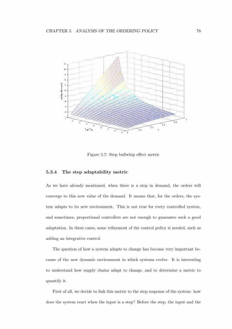
CHAPTER 5. ANALYSIS OF THE ORDERING POLICY 78
Figure 5.7: Step bullwhip effect metric
5.3.4 The step adaptability metric
As we have already mentioned, when there is a step in demand, the orders will
converge to this new value of the demand. It means that, for the orders, the sys-
tem adapts to its new environment. This is not true for every controlled system,
and sometimes, proportional controllers are not enough to guarantee such a good
adaptation. In these cases, some refinement of the control policy is needed, such as
adding an integrative control.
The question of how a system adapts to change has become very important be-
cause of the new dynamic environment in which systems evolve. It is interesting
to understand how supply chains adapt to change, and to determine a metric to
quantify it.
First of all, we decide to link this metric to the step response of the system: how
does the system react when the input is a step? Before the step, the input and the

CHAPTER 5. ANALYSIS OF THE ORDERING POLICY 79
output are constant values. When the input steps to a new value and if the system
is stable, the output converges to a constant value in a certain amount of time. We
decide to define the adaptability metric at 5% denoted adapt5% as the time since
when the output stays within the 5% interval around the new constant value. That
is,
|Out(t)−K|K
≤ 5%, ∀t ≥ adapt5%.
There are as many adaptability concepts as parameters. We can define the order
adaptability, the net stock adaptability, the work in process adaptability. Common
sense suggests that the adaptability should be as large as possible meaning that,
when dealing with variations, we want the system to adapt to the new situation,
and that it adapts as soon as possible. Obviously, this means that the time to adapt
should be as little as possible.
Let us describe the tradeoff at stake through an example. We will compare
two different sets of parameters. For both, we will consider a constant exponential
smoothing parameter α = 0.3 and a constant lead time LT = 10. For the first system
(in red), we set TWIP = TNS = 3 whereas the second one (in green) implements the
setting TWIP = TNS = 8. The results for the Net Stock, the WIP and the Orders
are presented in figures 5.8, 5.9, 5.10.
We observe how more adaptive the first system is in the sense of the definition
we have just given. It takes less time for the red system to ‘reach’ its limit. Being
adaptive for a supply chain means that it is capable of coping with long-run changes
quickly, which is most valuable in today’s competitive environment. The respon-
siveness deals with rapid changes, as opposed to the adaptability which is related to
long-run changes. These two concepts are complementary and encompass the more

CHAPTER 5. ANALYSIS OF THE ORDERING POLICY 80
Figure 5.8: Comparison of Net Stock answers to an aggressive and a smooth ordering
policies
Figure 5.9: Comparison of WIP answers to an aggressive and a smooth ordering
policies

CHAPTER 5. ANALYSIS OF THE ORDERING POLICY 81
Figure 5.10: Comparison of Orders answers to an aggressive and a smooth ordering
policies
global concept of flexibility.
Let us see now what this adaptability metric looks like when we make the ad-
justing parameters and the exponential smoothing parameter vary (the lead time is
equal to LT = 10). It is shown on figure 5.11.
Figure 5.11: The step adaptability metric

CHAPTER 5. ANALYSIS OF THE ORDERING POLICY 82
In terms of variations, we see that the lower the adjusting parameters and the
higher the smoothing constant, the better the adaptability. It is the same conclusion
as for the step responsiveness metric.
One could ask the question of the existence of any correlation between the adapt-
ability and the responsiveness concepts. From our study, by comparing the two
curves, it seems that being responsive also means being adaptive. This is most
probably the case for our system. But the definitions are definitely not the same
and we can figure out a system where the two concepts are uncorrelated.
5.4 Understanding and compromising the bullwhip ef-
fect and the flexibility
During the first part of the analysis, we have mainly studied the bullwhip effect and
what we called the flexibility. From our point of view, the flexibility encompasses
the responsiveness and adaptability issues. We have also given ways to quantify
these concepts. We would like to add two more things.
The first thing deals with the different metrics we have given to calculate the
bullwhip effect. Indeed, we have given metrics for different kinds of demand patterns:
the sine wave, the i.i.d demand and the step. But, in the case where the demand can
be modeled with these three modeling patterns, each one can be studied separately,
and this analysis provides a better understanding of the bullwhip effect formation.
It is possible to understand where it really comes from and to act accordingly if
possible. In other words, we can answer questions such as:
• How does the seasonality and the stochasticity contribute to the bullwhip
effect?

CHAPTER 5. ANALYSIS OF THE ORDERING POLICY 83
• How does my system react to steps? Then, what about the bullwhip effect
and the flexibility of my system?
• How can I quantify these effects?
From that perspective, we believe that this first part of the study has enlarged and
refined the bullwhip effect topic.
The second thing is relative to our system. We would like to highlight the tradeoff
that we have observed between having a weak bullwhip effect and being flexible.
The bullwhip effect and the flexibility are two important components of the supply
chain. When considering our system and the associated ordering policy, we fall
upon a tradeoff between these two parameters. Indeed, if we want a weak bullwhip
effect, we need to set large adjusting parameters in order to smooth the orders as
much as possible. This smoothed order pattern faced by an upstream echelon of
the supply chain will be less costly. However, doing so can be problematic in the
sense that the flexibility is endangered. We have understood the flexibility as the
ability of the supply chain to cope with change. It will take some time to the supply
chain to respond and to adapt to changes. Supply chain managers should have this
tradeoff in mind so as to take these two dimensions into account when making their
decisions.
To shed more light on this tradeoff, we present a graph mixing together the
different metrics. Since the metrics are not really related to each other, we have
linearly standardised the data to make them fit into a scale from zero to one. Here
is the result in figure 5.12.
We can read on this graph that, in order to get a weak bullwhip effect, supply
chain managers should implement smooth policies corresponding to large adjusting

CHAPTER 5. ANALYSIS OF THE ORDERING POLICY 84
Figure 5.12: Bullwhip effect, responsiveness, adaptability: compromising
parameters and a low exponential smoothing parameter, but this is at the expense of
the responsiveness and the adaptability. Conversely, if there is a need for flexibility,
managers should privilege aggressive policies with small adjusting parameters and
a small exponential smoothing parameter knowing that there will be a detrimental
impact on the bullwhip effect. This graph can be used to understand and compro-
mise the effects of the implemented policy on the bullwhip effect and the flexibility
of the supply chain.
So far, we have analysed our system from the adjusting and exponential smooth-
ing parameters point of view. There is actually a very important parameter we
already talked about in the literature review: the lead time. We mentioned its rel-
ative importance to the dynamics of the system. Before analysing the effect of the
lead time, we just want to recall what Sterman said about it:
CHAPTER 5. ANALYSIS OF THE ORDERING POLICY 85
‘Oscillation arises from the combination of time delays in negative feed-
backs and failure of the decision maker to take the time delays into
account.’
5.5 Effect of the lead time
Let us analyse the effect of the lead time on the system. What happens if we
increase or decrease the lead time? Here arises the question of the time compression
mentioned in the literature review as a principle for bullwhip effect reduction. In
order to have a weak bullwhip effect, each activity should take the minimum amount
of time. For our system, this assertion reduces to having a minimum lead time since
it corresponds to the only activity that takes time (the lead time can consist of a
transportation or production delay). Let us study the influence of the lead time on
the metrics.
5.5.1 Lead time and Bode diagrams
In the following figure, we present the transfer function O(z)D(z) for three different values
of the lead time: LT ∈ [4, 7, 10]. The other values are constant: TWIP = 4, TNS = 4,
α = 0.3.
The graph suggests that for any value of the frequency, the magnitude of the
transfer function increases when the lead time increases. The value of the magnitude
is a measure for the bullwhip effect as we saw it in section 5.2.1. This being said
and remembering that any time series can be decomposed into frequency series, it
means that, for any demand signal, the lower the lead time, the weaker the bullwhip
effect.
To prove this result, we have to prove that the absolute value of the magnitude of

CHAPTER 5. ANALYSIS OF THE ORDERING POLICY 86
Figure 5.13: Effect of the lead time on the orders
the transfer function is an increasing function of the lead time when the variable z
describes the unit circle (z = ejω).∣∣∣∣O(z)D(z)
∣∣∣∣ =
∣∣∣∣∣ (TWIP + LT + TWIPTNS
(1 + Ta))− z−1(TWIP + LT + TWIPTNS
Ta)
(1 + Ta − Taz−1)(TWIP + z−1(1− TWIP ) + z−LT−1(TWIPTNS
− 1))
∣∣∣∣∣∝
∣∣∣∣∣(TWIP + LT + TWIPTNS
(1 + Ta))− z−1(TWIP + LT + TWIPTNS
Ta)
TWIP + z−1(1− TWIP ) + z−LT−1(TWIPTNS
− 1)
∣∣∣∣∣(5.17)
The numerator is quite obviously an increasing function of LT , whereas we can-
not conclude anything regarding the denominator unless we set TWIP = TNS which
makes this denominator independent from the lead time. We have already said that
this assumption would be made in our study.
If we make the assumption TWIP = TNS , then the absolute value of the magni-
tude of the transfer function is an increasing function of the lead time. This proves
that the smaller the lead time, the weaker the bullwhip effect, at any frequencies.
We can exactly quantify the contribution of a lead time decrease to the seasonality
bullwhip effect. This can be useful when it comes to implementing bullwhip effect

CHAPTER 5. ANALYSIS OF THE ORDERING POLICY 87
reduction programs with the decrease of the lead time being one of the incentives.
5.5.2 Lead time and independent and identically distributed de-
mand
While looking at the formula we derived for the bullwhip effect of our system facing
an i.i.d demand (see 5.6), we easily figure out that the lead time only appears at the
numerator. But it is not easy to see how an increase of the lead time affects this
metric.
This metric can be written in the following way:
a ∗ (LT + TWIP )2 + b ∗ (1 + Ta + LT )2 − c ∗ (LT + TWIP )(1 + Ta + LT ), (5.18)
with a > 0, b > 0 , c > 0. It simplifies to a second degree polynomial except for
singular cases. We could get into the study of this polynomial but we preferred to
do it computationally within the range of interest. For three different exponential
smoothing parameters α = 0.1, 0.2, 0.3, for adjusting parameters ranging from 1 to
10, we made the lead time vary from 5 to 15 to see its influence, which was expected
to be quadratic in the lead time. Here are the results:
As we said before, with a view to decreasing the bullwhip effect, it is important
to understand and quantify (when it is possible) the contribution of the lead time.
How sensitive this metric is to the lead time is also important and can be appreciated
on the graph. For example, we can say that decreasing the lead time by one unit
seems to be less efficient than decreasing the proportional controllers by one unit.
Such a suggestion comes to mind when observing how sensitive to the parameters
the i.i.d bullwhip effect metric is. Here again, the possibility of quantifying the effect

CHAPTER 5. ANALYSIS OF THE ORDERING POLICY 88
Figure 5.14: Effect of the lead time on the iid bullwhip effect metric with α = 0.1
Figure 5.15: Effect of the lead time on the iid bullwhip effect metric with α = 0.2

CHAPTER 5. ANALYSIS OF THE ORDERING POLICY 89
Figure 5.16: Effect of the lead time on the iid bullwhip effect metric with α = 0.3
of the decisions proves advantageous.
5.5.3 Lead time and step response
We defined bullwhip effect and flexibility metrics when the system faces a step of
demand. The step responsiveness metric has been defined by the time when the
orders step response reaches its maximum. For the purpose of this section, we can
write this metric as a function of the lead time. The step responsiveness metric can
be written:
n = c1 +ln( 1+LT+Ta
LT+TWIP)
ln( Ta1+Ta
)− ln(TWIP−1TWIP
), (5.19)
where c1 ∈ R is independent from the lead time.
Using the fact that the logarithm function is concave, we prove that the metric is
a decreasing function of the lead time. This result is interesting since it follows the
intuition. Moreover, we can deduct the marginal contribution of a decrease of the
lead time over the step responsiveness metric.

CHAPTER 5. ANALYSIS OF THE ORDERING POLICY 90
5.6 The profit issue
As mentioned before, the profit is an important issue and is very often seen as what
eventually matters. When all the orders are fulfilled, then the profit is defined as
the sum of the cash flows which are defined as follows:
CashF lowt = Psale ∗Dt − Ppur ∗Rt − h ∗NSt. (5.20)
If the unit costs and prices are constant, then we get the expected cash flow:
E(CashF lowt) = Psale ∗ E(Dt)− Ppur ∗ E(Rt)− h ∗ E(NSt). (5.21)
We can also get the transfer function of the cash flow over the demand since:
CashF low(z) = Psale ∗D(z)− Ppur ∗R(z)− h ∗NS(z),
yielding to:
CashF low(z)D(z)
= Psale − Ppur ∗R(z)D(z)
− h ∗ NS(z)D(z)
= Psale − Ppur ∗ z−LT−1 ∗ O(z)D(z)
− h ∗ NS(z)D(z)
,
(5.22)
where the two transfer functions O(z)D(z) and NS(z)
D(z) have already been calculated
earlier. This enables us to study some characteristics of this profit function.
5.6.1 Profit and independent and identically distributed demand
If the demand is independent and identically distributed, then the expected cash
flow is:
E(CashF lowt) = Psale ∗ E(Dt)− Ppur ∗ E(Rt)− h ∗ E(NSt),

CHAPTER 5. ANALYSIS OF THE ORDERING POLICY 91
which, since all the means do not depend upon time (stationarity) and E(D) =
E(R) = E(O), yields to:
E(CashF lowt) = Psale ∗ E(D)− Ppur ∗ E(R)− h ∗ E(NS)
= (Psale − Ppur) ∗ E(D)− h ∗ E(NS).
(5.23)
The expected cash flow can be increased by lowering the target net stock level,
but this would endanger the service level since the probability for a shortage would
be higher. This is a well-known stationary result, let’s now study how transitory
dynamics work, when the system faces a step in demand.
5.6.2 The profit step response
Let us first study the step response. Unfortunately, because of the form of the
cash flow transfer function which is too complex, we cannot get the analytical cash
flow function. The next figure shows two such responses with the parameters being
α = 0.2, TWIP = TNS = 4, h = 10$/unit, Psale = 100$/unit, Ppur = 80$/unit for
the red curve, and by increasing the adjusting times by two units for the black curve
(TWIP = TNS = 6):
In this case, the step is a positive step-the demand increases, which explains
why the cash flow gets positive. The curve shown is a difference curve, it shows the
difference with the equilibrium state before the step. Since the difference between
the sales price and the purchasing price is equal to 20$, it is normal that the profit
tends to this limit. What is interesting to notice is the transitory dynamics. During
the first ten periods, there is no change since the new orders are not taken into
account yet. The greater profit is the result of a higher demand and of a linear
decreasing of the net stock, which linearly decreases the holding expenses. The
interesting part is next, when the policy starts to play its role, and this is the part

CHAPTER 5. ANALYSIS OF THE ORDERING POLICY 92
Figure 5.17: Cash Flow response to a unit step in demand with different adjusting
times
we are going to focus on. After the lead-time period, the least aggressive policy
seems to offer a greater profit. This is mainly explained by a lower net stock during
this phase, inducing a lower holding cost as it has been demonstrated earlier. The
two net stock responses are presented below:
Since the orders are paid at the receipt, we must not forget to translate the
orders curve of the lead time. When observing the curves, we conclude that, in the
case of a positive step in the demand, the more aggressive the policy is, the more the
holding cost is. It is different with the orders since they are greater and then lesser,
and vice versa, for two different policies. Let us indeed calculate the purchasing
costs during this transitory phase.
We calculated the orders response previously:
Z−1(O(z))(n) =1(n) +Ta(LT + TWIP )
(1 + Ta)(1 + Ta − TWIP )∗(
Ta1 + Ta
)n∗ 1(n)
+(1− TWIP )(1 + LT + Ta)TWIP (1 + Ta − TWIP )
∗(
1− 1TWIP
)n∗ 1(n)
The purchasing costs PurCost, over an infinite horizon, are equal to the sum of

CHAPTER 5. ANALYSIS OF THE ORDERING POLICY 93
Figure 5.18: Net Stock response to a unit step in demand with different adjusting
times
Figure 5.19: Orders response to a unit step in demand with different adjusting times

CHAPTER 5. ANALYSIS OF THE ORDERING POLICY 94
a constant term due to the new equilibrium and a difference term which can make
the difference. This difference term ˜PurCost is equal to:
˜PurCost =+∞∑n=0
Ppur ∗ (On − 1(n))
= Ppur ∗+∞∑n=0
(On − 1(n))
= Ppur ∗+∞∑n=0
[ Ta(LT + TWIP )(1 + Ta)(1 + Ta − TWIP )
∗(
Ta1 + Ta
)n+
(1− TWIP )(1 + LT + Ta)TWIP (1 + Ta − TWIP )
∗(
1− 1TWIP
)n]= Ppur ∗
[ Ta(LT + TWIP )(1 + Ta − TWIP )
+(1− TWIP )(1 + LT + Ta)
(1 + Ta − TWIP )
]= Ppur ∗
Ta(1 + LT )− TWIP (1 + LT ) + 1 + LT
1 + Ta − TWIP
= Ppur ∗ (1 + LT )
(5.24)
This term is constant (independent of the ordering policy), and actually corre-
sponds to the missed orders during the lead time period after the step. The step
appears at period, say n0. Then the orders will change only at the end of the period
n0, and the first modified order will arrive at the beginning of the period n0+LT+1.
Hence, since the step is a unit step, the number of missed orders is indeed equal to
LT + 1. This result could have actually been predicted since:
• it is normal to compensate for the missed orders,
• a difference between the two policies would have meant that orders were lost.
To conclude on the profit issue, we can say that in the case of a step increase of
demand, the only leverage we have is the holding costs, and the ordering policy does
not affect the profit on the long run. Then, smoother policies will be less costly since
the net stock will converge to its new target level more slowly. What if the change
in demand is a step decrease? Just the opposite. The more aggressive policies will

CHAPTER 5. ANALYSIS OF THE ORDERING POLICY 95
be more cost-effective for the opposite reason. It would then be relevant to predict
if the demand is about to increase or decrease, and to define the ordering policy
accordingly.

Chapter 6
Conclusion
The aim of the study was to define a model of an ordering policy, and to analyse its
dynamic behaviour using the theoretical framework of control theory.
First of all, we have come up with an efficient model for simulations. This single-
stage model is based on control theory concepts such as the feedback and takes the
lead time into account. The proportional controllers and the exponential smoothing
forecast constant are the two parameters we built our analysis upon.
The analysis was aimed at studying the dynamic behaviour of the system facing
different demand situations. The three dynamic demand situations were the sine
wave, the step and the independent and identically distributed random variable.
From there, we came up with an analysis of the two supply chain concepts of bull-
whip effect and flexibility.
The bullwhip effect is a well-known phenomenon and corresponds to an amplifi-
cation of the variations of the orders along the chain, from the retailers to the raw
96

CHAPTER 6. CONCLUSION 97
material suppliers. Our analysis has defined bullwhip effect metrics for the three
different dynamic demand situations.
The flexibility is a concept which has lately gained a lot of consideration to de-
termine a supply chain’s performance. We defined it as the ability of the supply
chain to cope with change. The responsiveness and the adaptability are the two
quantitative concepts that emerged from our study.
With regards to these two supply chain issues, the interest of our work is twofold:
• studying these phenomena from different dynamic perspectives,
• defining metrics which enable for a quantitative study.
Our study shows that a compromise must be made between having a weak bull-
whip effect and being flexible. The metrics we defined can help supply chain man-
agers make consistent decisions based on quantitative facts, according to how they
want to compromise the bullwhip effect and the flexibility.
We also studied how the lead time affects the system’s performance, from a struc-
tural point of view with the explanation of oscillations, and from a quantitative point
of view with its effect on the metrics. A profit function was also introduced and gives
elements on how to choose between an aggressive and a smooth policy.
One important point of this conclusion deals with the improvements and devel-
opments that can be made. We have pointed out two very promising directions in
the right continuation of this study.
The first one has to do with the situation of shortages. Our model allows for
shortages and we carried out simulations to understand the phenomenon. But a
proper analysis would be more relevant and would provide more accurate results.

CHAPTER 6. CONCLUSION 98
The theory which should support such an analysis is non-linear control theory.
The second direction would be a generalisation of our model, with the use of
adaptive control. Instead of having fixed proportional controllers and exponential
smoothing constant, we can design a system where these parameters change every
time period, according to some performance criteria. For instance, the criteria can
be purely profit-based, or defined as a function of the bullwhip effect and the flexi-
bility metrics.
The last point of this conclusion deals with a personal reflection regarding the
demand control itself. The bullwhip effect is a response of the supply chain system
to an uncontrolled demand change. Why not try to control the demand, at least to
some point? Why not take a more global perspective of the supply chain system,
making the demand an endogenous parameter? This is tantamount to making the
final consumers part of the supply chain system. For instance, a supply chain policy
including the marketing incentives would certainly lead to better performance. Ef-
forts have already been made in the literature to the definition of joined pricing and
ordering strategies. But the method chosen so far is the maximisation of a profit
function which cannot cope with lead times, which are inherent to supply chains.
The use of control theory would probably lead to new significant results. The idea
would consist of defining a new feedback on the demand, the marketing incentives
(pricing, promotion...) being the means of the company to act upon the demand.
This is coordination of the marketing and ordering policies in a dynamic environ-
ment. It would possibly allow for the demand change to be less abrupt and less
ample, since more controlled, leading naturally to a reduction of the bullwhip effect.
Our intuition is that using such a feedback would make the system perform better in

CHAPTER 6. CONCLUSION 99
terms of bullwhip effect and flexibility, and eventually profit. Put in systems think-
ing and control theory terms, the final consumers become part of the system and
provide more informed and useful feedback for a better performance of the system.

Bibliography
[1] D. Simchi-Levi, E. Simchi-Levi, and P. Kaminsky. Designing and managing the
supply chain - Concepts, strategies and case studies. Mc Graw-Hill, 2003.
[2] K. O’Marah. The leaders’ edge: Driven by demand. Supply Chain Management
Review, 2005.
[3] M. Ortega and L. Lin. Control theory applications to the production-inventory
problem: a review. International Journal of Production Economics, 1996.
[4] Supelec Collectif Automatique. Automatique. Imprimerie Supelec, 2004.
[5] G. Stalk and T.M. Hout. Time-the next source of competitive advantage. Har-
vard Business Review, 1988.
[6] J.D. Sterman. Business dynamics, Systems thinking for a complex world. Mc
Graw-Hill, 2000.
[7] H.A. Simon. On the application of servomechanism theory in the study of
production control. Econometrica, 1952.
[8] J.H. Vassian. Application of discrete variable servo theory to inventory control.
Operations Research, 1955.
100

BIBLIOGRAPHY 101
[9] S. Axsater. Control theory concepts in production and inventory control. In-
ternational Journal of Systems Science, 1985.
[10] D.R. Towill. Dynamic analysis of an inventory and order based production
control system. International Journal of Production Research, 1982.
[11] H.L. Lee, V. Padmanabhan, and S. Whang. The bullwhip effect in supply
chains. Sloan Management Review, 1997.
[12] S. Geary, S.M. Disney, and D.R. Towill. On bullwhip in supply chains-historical
review, present practice and expected future impact. International Journal of
Production Economics, 2006.
[13] D.M. Upton. Process range in manufacturing: an empirical study of flexibility.
Management Science 43, 1982.
[14] H.L. Lee. The triple-a supply chain. Harvard Business Review on Supply Chain
Management, 2006.
[15] J. Wikner. Dynamic modeling and analysis of information flows in production-
inventory and supply chain systems. Journal of Systems Engineering, 1994.
[16] J. Dejonckheere, S.M. Disney, M.R. Lambrecht, and D.R. Towill. Measuring and
avoiding the bullwhip effect: a control theoretic approach. European Journal
of Operational Research, 2003.
[17] J.W. Forrester. Industrial Dynamics. MIT Press, 1961.
[18] H.I. Ansoff and D.P. Slevin. An appreciation of industrial dynamics. Manage-
ment Science, 1968.

BIBLIOGRAPHY 102
[19] R.W. Grubbstrom and J. Wikner. Inventory trigger control policies developed
in terms of control theory. International Journal of Production Economics,
1996.
[20] J. Antoine, J. Colette, G. Duc, H. Gueguen, and D. Poulton. Signaux et Sys-
temes. Imprimerie Supelec, 2002.
[21] V.J. Bucek. Control Systems, Continuous and Discrete. Prentice Hall, 1989.
[22] Y. Z. Tsypkin. Sampling systems theory and its application. Pergamon Press,
Oxford, 1964.