dynamical systems as temporal feature spaces
TRANSCRIPT
Journal of Machine Learning Research 21 (2020) 1-42 Submitted 7/19; Revised 12/19; Published 2/20
Dynamical Systems as Temporal Feature Spaces
Peter Tino [email protected]
School of Computer Science
University of Birmingham
Birmingham, B15 2TT, UK
Editor: Sayan Mukherjee
Abstract
Parametrised state space models in the form of recurrent networks are often used in machinelearning to learn from data streams exhibiting temporal dependencies. To break the blackbox nature of such models it is important to understand the dynamical features of the input-driving time series that are formed in the state space. We propose a framework for rigorousanalysis of such state representations in vanishing memory state space models such as echostate networks (ESN). In particular, we consider the state space a temporal feature spaceand the readout mapping from the state space a kernel machine operating in that featurespace. We show that: (1) The usual ESN strategy of randomly generating input-to-state, aswell as state coupling leads to shallow memory time series representations, correspondingto cross-correlation operator with fast exponentially decaying coefficients; (2) Imposingsymmetry on dynamic coupling yields a constrained dynamic kernel matching the inputtime series with straightforward exponentially decaying motifs or exponentially decayingmotifs of the highest frequency; (3) Simple ring (cycle) high-dimensional reservoir topologyspecified only through two free parameters can implement deep memory dynamic kernelswith a rich variety of matching motifs. We quantify richness of feature representationsimposed by dynamic kernels and demonstrate that for dynamic kernel associated withcycle reservoir topology, the kernel richness undergoes a phase transition close to the edgeof stability.
Keywords: Recurrent Neural Network, Echo State Network, Dynamical Systems, TimeSeries, Kernel Machines
1. Introduction
When dealing with time series data, techniques of machine learning and signal processingmust account in some way for temporal dependencies in the data stream. One popularoption is to impose a parametric state-space model structure in which the state vector issupposed to dynamically code for the input time series processed so far and the outputis determined through a static readout from the state. Recurrent neural networks (e.g.(Downey et al., 2017)), Kalman filters (Kalman, 1960) or hidden Markov models (Baumand Petrie, 1966) represent just a few examples of this approach. In some cases the statespace and transition structure is (at least partially) imposed based on the relevant priorknowledge (Yoon, 2009), but usually it is learnt from the data along with the readoutmap. In the case of uncountable state space and non-linear state dynamics, the use ofgradient methods in learning the state transition dynamics is hampered by the well known
c©2020 Peter Tino.
License: CC-BY 4.0, see https://creativecommons.org/licenses/by/4.0/. Attribution requirements are providedat http://jmlr.org/papers/v21/19-589.html.
Peter Tino
“information latching problem” (Bengio et al., 1993). As temporal sequences increase inlength, the influence of early components of the sequence have less impact on the networkoutput. This causes the partial gradients, used to update the weights, to (exponentially)shrink to zero as the sequence length increases. Several approaches have been suggested toovercome this challenge, e.g. (Bengio et al., 1994; Hochreiter and Schmidhuber, 1997; Jinget al., 2019).
One possibility to avoid having to train the state transition part in a state space modelis to simply initialise it randomly to a ‘sensible’ fading memory dynamic filter and onlytrain the static readout part of the model. Models following this philosophy (Jaeger, 2001;Maass et al., 2002; Tino and Dorffner, 2001) have been termed “reservoir computation (RC)models” (Lukosevicius and Jaeger, 2009). Perhaps the simplest form of a RC model is theEcho State Network (ESN) (Jaeger, 2001, 2002a,b; Jaeger and Hass, 2004). Briefly, ESNis a recurrent neural network with a non-trainable state transition part (reservoir) and asimple trainable linear readout. Connection weights in the ESN reservoir, as well as theinput weights are randomly generated. The reservoir weights are scaled so as to ensure the“Echo State Property” (ESP): the reservoir state is an “echo” of the entire input history anddoes not depend on the initial state. Scaling reservoir weights so that the largest singularvalue is smaller than 1 makes the reservoir dynamics contractive and guarantees the ESP. Inpractice, sometimes it is the spectral radius that guides the scaling. In this case, however,spectral radius < 1 does not guarantee the ESP.
ESNs has been successfully applied in a variety of tasks (Jaeger and Hass, 2004; Skowron-ski and Harris, 2006; Bush and Anderson, July 2005; Tong et al., 2007). Many extensionsof the classical ESN have been suggested in the literature, e.g. deep ESN (Gallicchio et al.,2017), intrinsic plasticity (Schrauwen et al., 2008; Steil, 2007), decoupled reservoirs (Xueet al., 2007), leaky-integrator reservoir units (Jaeger et al., 2007), filter neurons with delay-and-sum readout (Holzmann and Hauser, 2009) etc. However, there are properties of thereservoir that are poorly understood (Xue et al., 2007) and specification of the reservoir andinput connections require numerous trails and even luck (Xue et al., 2007). Furthermore,imposing a constraint on spectral radius or largest singular value of the reservoir matrix isa weak tool to properly set the reservoir parameters (Ozturk et al., 2007). Finally, randomconnectivity and weight structure of the reservoir is unlikely to be optimal and such a set-ting prevents us from providing a clear and systematic insight into the reservoir dynamicsorganisation (Ozturk et al., 2007; Rodan and Tino, 2010). Rodan and Tino (2010) demon-strated that even an extremely simple setting of a high-dimensional state space structuregoverned by only two free parameters set deterministically can yield modelling capabilitieson par with other ESN architectures. However, a deeper understanding of why this is sohas been missing.
In order to theoretically understand the workings of parametrised state space modelsas machine learning tools to process and learn from temporal data, there has been a livelyresearch activity to formulate and assess different aspects of computational power and infor-mation processing capacity in such systems (e.g. (Dambre et al., 2012; Obst and Boedecker,2014; Hammer, 2001; Hammer and Tino, 2003; Siegelmann and Sontag, 1994; Tino andHammer, 2004)). For example, tools of information theory have been used to assess infor-mation storage or transfer within systems of this kind (Lizier et al., 2007, 2012; Obst et al.,2010; Bossomaier et al., 2016). To specifically characterise capability of input-driven dy-
2
Dynamical Systems as Temporal Feature Spaces
namical systems to keep in their state-space information about past inputs, several memoryquantifiers were proposed, for example “short term memory capacity” (Jaeger, 2002a) and“Fisher memory curve” (Ganguli et al., 2008; Tino, 2018). Even though those two measureshave been developed from completely different perspectives, deep connections exist betweenthem (Tino and Rodan, 2013). The concept of memory capacity, originally developed forunivariate input streams, was generalised to multivariate inputs in (Grigoryeva et al., 2016).Couillet et al. Couillet et al. (2016) rigorously studied mean-square error of linear dynami-cal systems used as dynamical filters in regression tasks and suggested memory quantitiesthat generalise the short term memory capacity and Fisher memory curve measures. Fi-nally, Ganguli and Sompolinsky (2010) showed an interesting connection between memoryin dynamical systems and their capacity to perform dynamical compressed sensing of pastinputs.
In this contribution, we suggest a novel framework for characterising richness of dynamicrepresentations of input time series in the form of states of a dynamical system, which is thecore part of any state space model used as a learning machine. Our framework is based onthe observation that the idea of fixed dynamic reservoir with simple static linear mappingbuild on top of it strikingly resembles the philosophy of kernel machines (Legenstein andMaass, 2007). There, the inputs are transformed using a fixed mapping (usually onlyimplicitly defined) into a feature space that is ”rich enough” so that in that space it issufficient to train linear models only. The key tool for building linear models in the featurespace is the inner product. One can grasp workings of a kernel machine by understandingof how the data is mapped to the feature space and what ”data similarity” in the originalspace means when expressed as the inner product in the feature space. We will view thereservoir state space as a ”temporal feature space” in which the linear readout is operating.In this view, the input time series seen by the reservoir model results in a state that codesall history of the presented input items so far and thus forms a feature representation ofthe time series. Different forms of coupling in the reservoir dynamical system will result indifferent temporal feature spaces with different feature representations of input time series,implying different notions of similarity between time series, expressed as inner products oftheir feature space representations. We will ask if and how the feature spaces differ in casesof traditional randomly generated reservoir models, as well as more constrained reservoirconstructions studied in the literature.
Since RC models are input-driven non-autonomous dynamical systems, theoretical stud-ies linking their information processing capabilities to the reservoir coupling structures havebeen performed mostly in the context of linear dynamics, e.g. (Ganguli et al., 2008; Couil-let et al., 2016; Couillet et al., 2016; Tino, 2018). While such studies are of interest bythemselves, in the context of the present work, studying linear dynamics can shed lighton a wide class of RC models whose approximation capabilities equal those of non-linearsystems. In particular, Grigoryeva, Gonon and Ortega recently proved a series of importantresults concerning universality of RC models (Grigoryeva and Ortega, 2018b,a; Gonon andOrtega, 2019). The universality can be obtained even if the state transition dynamics islinear, provided the readout map is polynomial (or a neural network)1. However, univer-
1. Universal approximation capability was first established in the L∞ sense for deterministic, as well asalmost surely uniformly bounded stochastic inputs (Grigoryeva and Ortega, 2018b). This was later
3
Peter Tino
sality is a property of a whole family of RC models. For appropriate classes of filters2 andinput sources, it guarantees that for any filter and approximation precision, there exists aRC model approximating the filter to that precision. This is an existential statement thatdoes relate individual filters to their approximating RC models. Our new framework willenable us to reason about what kind of RC model setup is necessary if filters with deepermemory were to be approximated. In particular, we will first investigate properties of lineardynamical readout kernels obtained on top of linear dynamical systems. Crucially, memoryproperties of such kernels can not be enhanced by moving from linear to polynomial staticreadout kernels. Loosely speaking, if feature representation x of a time series u capturesproperties of u only up to some look-back time t− τ0 from the last observation time t, thenno nonlinear transformation γ of x can prolong memory τ0 in the feature representationγ(x) of u. Hence, we will be able to make statements regarding appropriate settings of thelinear dynamics that are necessary for universal approximation of deeper memory filters.
The paper has the following organisation: In section 2 we set the scene and outline themain intuitions driving this work. Section 3 formally introduces the notion of temporalkernel and provides some useful properties of the kernel to be used further in our study.In section 4 we will setup basic tools for characterising dynamic kernels - motifs and theircorresponding motif weights. Starting from section 5, we will analyse dynamic kernelscorresponding to different settings of the dynamical system. In particular, dynamical kernelsassociated with fully random, symmetric and highly constrained coupling of the dynamicalsystem are analysed in sections 5, 6 and 7, respectively. We provide examples illustratingthe developed theory and compare the motif richness of different parameter settings of thedynamical system in section 8. The paper finishes with discussion and conclusions in section9.
2. Preliminary concepts and intuitions
We consider fading memory state space models with linear input driven dynamics in an N -dimensional state space and univariate inputs and outputs. Note that in the ESN metaphor,the state dimensions correspond to reservoir units coupled to the input u(t) via an N -dimensional weight vector w ∈ RN . Denoting the state vector at time t by x(t) ∈ RN , thedynamical system evolves as
x(t) = W x(t− 1) + w u(t), (1)
where W ∈ RN×N is an N ×N weight matrix providing the dynamical coupling. In statespace models, the output y(t) is often determined solely based on the current state x(t)through a readout function h:
y(t) = h(x(t)). (2)
The readout map h is typically trained (offline or online) by minimising the (normalised)mean square error between the targets and reservoir readouts y(t).
extended in (Gonon and Ortega, 2019) to Lp, 1 ≤ p < ∞ and not necessarily almost surely uniformlybounded stochastic inputs.
2. transforming semi-infinite input sequences into outputs
4
Dynamical Systems as Temporal Feature Spaces
Denote the set of natural numbers (including zero) by N0. In this contribution, we studyhow the dynamical system (1) extracts potentially useful information about the left infiniteinput time series ..., u(t− 2), u(t− 1), u(t), u(−j) ∈ R, j ∈ N0, in its state x(t) ∈ RN , sinceit is only the state x(t) that will be used to produce the predictive output y(t) upon seeingthe input time series up to time t. In particular, we will consider readout maps constructedin the framework of kernel machines. For example, in the case of linear Support VectorMachine (SVM) regression, the readout from the state space at time t has the form
y(t) = h(x(t)) =∑i
βi 〈x(ti),x(t)〉+ b, (3)
where βi ∈ R and b ∈ R are weight coefficients and bias term, respectively and x(ti) aresupport state vectors observed at important “support time instances” ti. In the spiritof state space modelling discussed above, we consider the state x(t′) ∈ RN reached afterobserving the time series ..., u(t′ − 2), u(t′ − 1), u(t′), the feature state space representationof that time series. Hence (3) can also be written as
y(t) =∑i
βi K([...u(ti − 1), u(ti)], [...u(t− 1), u(t)]) + b, (4)
where K(·, ·) is a time series kernel associated with the dynamical system (1),
K([...u(ti − 1), u(ti)], [...u(tj − 1), u(tj)]) = 〈x(ti),x(tj)〉 . (5)
In this context, the support time instances ti can be viewed as end times of the “supporttime series” ..., u(ti − 2), u(ti − 1), u(ti) observed in the past and deemed “important” forproducing the outputs by the training algorithm trained on the history of the time seriesbefore the time step t.
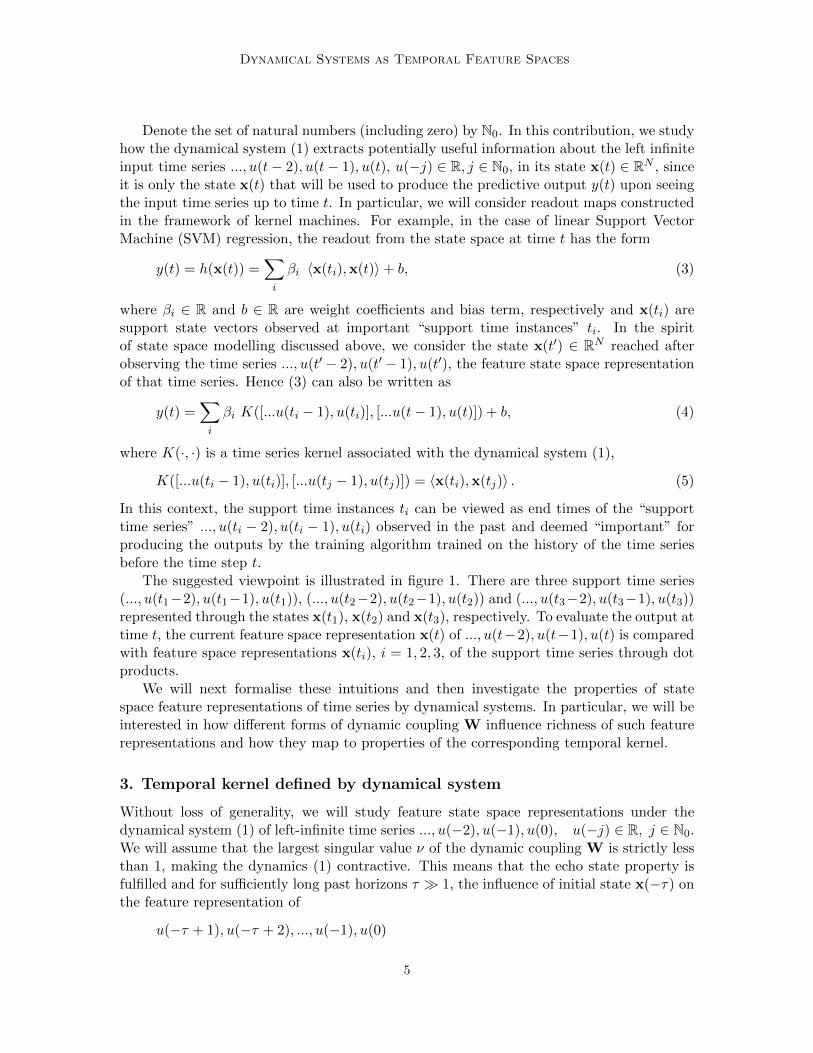
The suggested viewpoint is illustrated in figure 1. There are three support time series(..., u(t1−2), u(t1−1), u(t1)), (..., u(t2−2), u(t2−1), u(t2)) and (..., u(t3−2), u(t3−1), u(t3))represented through the states x(t1), x(t2) and x(t3), respectively. To evaluate the output attime t, the current feature space representation x(t) of ..., u(t−2), u(t−1), u(t) is comparedwith feature space representations x(ti), i = 1, 2, 3, of the support time series through dotproducts.
We will next formalise these intuitions and then investigate the properties of statespace feature representations of time series by dynamical systems. In particular, we will beinterested in how different forms of dynamic coupling W influence richness of such featurerepresentations and how they map to properties of the corresponding temporal kernel.
3. Temporal kernel defined by dynamical system
Without loss of generality, we will study feature state space representations under thedynamical system (1) of left-infinite time series ..., u(−2), u(−1), u(0), u(−j) ∈ R, j ∈ N0.We will assume that the largest singular value ν of the dynamic coupling W is strictly lessthan 1, making the dynamics (1) contractive. This means that the echo state property isfulfilled and for sufficiently long past horizons τ � 1, the influence of initial state x(−τ) onthe feature representation of
u(−τ + 1), u(−τ + 2), ..., u(−1), u(0)
5
Peter Tino
timet3t2t1
x( )x( ) x( )
tt t
tx( )
t
1
2 3
Figure 1: Illustration of the workings of kernel machine producing an output at time t afterobserving ..., u(t − 1), u(t). The time series ..., u(t − 1), u(t) is compared withthe three support time series (..., u(ti − 1), u(ti)), i = 1, 2, 3, by evaluating dotproducts between their feature space representations x(t) and x(ti).
is negligible. Note that ν < 1 is a sufficient condition for the echo state property, but theproperty may actually be achieved under milder conditions, especially when particular inputstreams are considered (for formal treatment and further details see e.g. (Yildiz et al., 2012;Manjunath and Jaeger, 2013)). In this contribution we use ν < 1, since it allows us (1) toconsider arbitrary input streams over a bounded domain (the ESP is always guaranteed)and (2) to explicitly bound, in terms of properties of W, the norm of dynamical states, aswell as the extent to which the initial state influences the temporal kernel.
More formally, given a past horizon τ � 1, we will represent the time series u(−τ +1), u(−τ + 2), ..., u(−1), u(0) as a vector u(τ) = (u1, u2, ..., uτ )> ∈ Rτ , where ui = u(−i +1), i = 1, 2, ...τ . In other words u(τ) = (u(0), u(−1), ..., u(−τ + 1))>.
Consider a state x(−τ) ∈ RN at time −τ . After seeing the input series u(−τ+1), u(−τ+2), ..., u(−1), u(0), the new state of the dynamics (1) will be3
x(0) = Wτx(−τ) +τ∑j=1
u(j − τ)Wτ−jw.
As discussed in the previous section, the state x(0) reached from the initial condition x(−τ)after seeing u(τ) codes for information content in u(τ) and will be considered the “featurespace representation” of u(τ) through the dynamical system (1):
φ(u(τ); x(−τ)) = x(0)
= Wτx(−τ) +τ∑i=1
u(1− i)Wi−1w
= Wτx(−τ) +
τ∑i=1
uiWi−1w. (6)
Given two time series at past horizon τ represented through u(τ) = (u1, u2, ..., uτ )> andv(τ) = (v1, v2, ..., vτ )>, the temporal kernel defined by dynamical system (1) evaluated on
3. W0 = IN×N , the N ×N identity matrix.
6
Dynamical Systems as Temporal Feature Spaces
u(τ) and v(τ) reads:
K(u(τ),v(τ); x(−τ)) = 〈φ(u(τ); x(−τ)), φ(v(τ); x(−τ))〉 . (7)
We will now show that, as expected given the contractive nature of (1), for sufficientlylong past time horizons τ � 1 on input streams over bounded domain4, the kernel evaluationis insensitive to the initial condition x(−τ). This will allow us to simplify the presentationby setting x(−τ) to the origin in the rest of the paper.
Theorem 1 Consider the dynamical system (1) driven by time series over a bounded do-main [−U,U ], 0 < U <∞, with a past time horizon τ > 1. Assume that the largest singularvalue ν of the dynamic coupling W is strictly smaller than 1 and that the norm of the inputcoupling w satisfies ‖w‖ ≤ B. Assume further that the norm of the initial condition isupper bounded by ‖x(−τ)‖ ≤ A(τ) = c · ζ−τ , where ν < ζ < 1 and c > 0 is a large enoughpositive constant satisfying
c ≥ B · U
(1− ν) ·(
1− νζ
) . (8)
Then, for any u(τ),v(τ) ∈ [−U,U ]τ , it holds
K(u(τ),v(τ); x(−τ)) = K(u(τ),v(τ); 0) + ε,
where
−ητ[
2c
1− ν·B · U
]≤ ε ≤ ητ
[c2 ητ +
2c
1− ν·B · U
], (9)
with η = ν/ζ < 1.
Proof Note that
φ(u(τ); x(−τ)) = Wτx(−τ) + φ(u(τ); 0)
and therefore, denoting
φ(u(τ); 0) =
τ∑i=1
uiWi−1w (10)
by φ0(u(τ)), we have
K(u(τ),v(τ); x(−τ)) = 〈Wτx(−τ) + φ0(u(τ)),Wτx(−τ) + φ0(v(τ))〉= ‖Wτx(−τ)‖22 + 〈Wτx(−τ), φ0(u(τ)) + φ0(v(τ))〉+ K(u(τ),v(τ); 0),
4. It is common in the ESN literature to consider input streams over a bounded domain (e.g. Jaeger(2001)). In the recent work on universality of ESNs Grigoryeva and Ortega (2018b) consider almostsurely uniformly bounded stochastic inputs. This is further relaxed in (Gonon and Ortega, 2019).
7
Peter Tino
where
K(u(τ),v(τ); 0) = 〈φ0(u(τ)), φ0(v(τ))〉
is the dynamic kernel evaluated using initial condition x(−τ) set to the origin 0. We have,
‖Wτx(−τ)‖22 ≤ ν2τ · (A(τ))2. (11)
Note that
〈Wτx(−τ), φ0(u(τ))〉 ≤ ‖Wτx(−τ)‖ · ‖φ0(u(τ))‖
and (see (10))
‖φ0(u(τ))‖ ≤τ∑i=1
νi−1 · U · ‖w‖
≤ B · U · 1
1− ν, (12)
yielding
〈Wτx(−τ), φ0(u(τ))〉 ≤ ντ
1− ν·A(τ) ·B · U.
We thus have
K(u(τ),v(τ); x(−τ)) = K(u(τ),v(τ); 0) + ε,
with
ε ≤ ντ[ντ (A(τ))2 +
2
1− ν·A(τ) ·B · U
].
To evaluate the lower bound on ε, note that
〈Wτx(−τ), φ0(u(τ))〉 ≥ −‖Wτx(−τ)‖ · ‖φ0(u(τ))‖
≥ −ντ
1− ν·A(τ) ·B · U.
Since, trivially, ‖Wτx(−τ)‖22 ≥ 0, we have
ε ≥ − 2ντ
1− ν·A ·B · U.
We have thus obtained,
−ντ[
2
1− ν·A(τ) ·B · U
]≤ ε ≤ ντ
[ντ (A(τ))2 +
2
1− ν·A(τ) ·B · U
],
which is equivalent to (9).
8
Dynamical Systems as Temporal Feature Spaces
In order to reconcile this setting with the dynamics (1), consider a past horizon τ + τ0for some additional look-back time τ0 ≥ 1. We require,
‖x(−τ)‖ ≤ A(τ) = c · ζ−τ and ‖x(−τ − τ0)‖ ≤ A(τ + τ0) = c · ζ−τ−τ0 .
But from the dynamics (1), we also have (see eqs.(6), (11) and (12)),
‖x(−τ)‖ ≤ ‖Wτ0 x(−τ − τ0)‖+B · U1− ν
≤ ντ0 ·A(τ + τ0) +B · U1− ν
. (13)
We would like the norm of the state x(−τ) reached from the initial state x(−τ−τ0) (boundedin norm by A(τ + τ0)) to be within the required bound A(τ). In other words, we would like
A(τ + τ0) · ντ0 +B · U1− ν
< c · ζ−τ (14)
to hold. Using A(τ + τ0) = c · ζ−τ−τ0 , we conclude that the inequality (14) holds when
c > ζτ · B · U(1− ν)
· 1
1−(νζ
)τ0 . (15)
Since 0 < η = ν/ζ < 1, for τ, τ0 ≥ 1,
ζτ · B · U(1− ν)
· 1
1− ητ0<
B · U(1− ν) · (1− η)
we have that the inequality (15) is definitely satisfied when
c >B · U
(1− ν) · (1− νζ ).
Theorem 1 formally states that because the dynamical system (1) is contractive, theinfluence of the initial condition x(−τ) on the kernel value K(u(τ),v(τ); x(−τ)) decaysexponentially with the past time horizon τ . For sufficiently long past time horizons τ � 1 wecan thus set x(−τ) = 0. Hence, in the rest of this study we will assume τ ≥ N and (unlessnecessary) we will drop specific reference to τ by writing u instead of u(τ) ∈ Rτ . In fact, itwill be easier to think of time horizons in units of N , so that τ = ` ·N , for some sufficientlylarge integer ` > 1. Furthermore, we will refer to φ(u(τ); 0) and K(u(τ),v(τ); 0) simplyas φ(u) and K(u,v), respectively.
9
Peter Tino
4. Temporal kernel and its motifs
In the previous section we established that the temporal kernel associated with dynamicalsystem (1) and acting on time series with past time horizon τ � 1 is defined as
K(u,v) = 〈φ(u), φ(v)〉 . (16)
In order to analyse the action of K(u,v) on time series u,v, we need to find its expressiondirectly in terms of u and v. The next theorem shows that there exists a matrix Q of rankat most N that acts as a metric tensor on a subspace of Rτ (of dimensionality at most N),so that K(u,v) can be expressed as a quadratic form u>Q v. This will allow us to studyproperties of K(u,v) by analysing the associated metric tensor Q.
Theorem 2 Consider the dynamical system (1) of state dimensionality N and a dynamiccoupling W with largest singular value 0 < ν < 1. Let K(u,v) (16) be the temporal kernelassociated with system (1). Then for any u,v ∈ Rτ ,
K(u,v) = u>Q v = 〈u,v〉Q ,
where Q is a symmetric, positive semi-definite τ × τ matrix of rank Nm = rank(Q) ≤ Nand elements
Qi,j = w>(W>
)i−1Wj−1 w, i, j = 1, 2, ..., τ. (17)
The upper bound on absolute values of Qi,j decays exponentially with increasing time indicesi, j = 1, 2, ..., τ , as
|Qi,j | ≤ νi+j−2 ‖w‖22. (18)
Proof First, we write
K(u,v) = 〈φ(u), φ(v)〉
=
⟨τ∑i=1
uiWi−1w,
τ∑j=1
vjWj−1w
⟩(eq. (10))
=
τ∑i,j=1
ui vj⟨Wi−1w,Wj−1w
⟩=
τ∑i,j=1
ui vj Qi,j
= u>Q v.
Second, φ(u) can be written as φ(u) = Φu, where Φ is an N × τ matrix whose i-thcolumn is equal to Wi−1w. Hence, K(u,v) = u>Φ>Φ v and Q = Φ>Φ is symmetricpositive semi-definite with rank at most N ≤ τ .
10
Dynamical Systems as Temporal Feature Spaces
Finally, since ‖Wiw‖ ≤ ‖Wi‖‖w‖ ≤ νi‖w‖, we have
|Qi,j | = |⟨Wi−1w,Wj−1w
⟩|
≤ ‖Wi−1w‖2 · ‖Wj−1w‖2≤ νi+j−2 ‖w‖22.
Note that K(·, ·) is a semi-inner product on Rτ . In other words, time series u ∈ ker (Q)from the kernel of the linear operator Q have zero length. It acts as an inner product in thequotient of Rτ by ker (Q), Rτ/ ker (Q) (image of Q). Since this distinction is not crucialfor our argumentation, in order not to unnecessarily complicate the presentation, (slightlyabusing mathematical terminology) we will refer to K(·, ·) as temporal kernel and to Q asthe associated metric tensor.
Theorem 2 tells us that K(·, ·) is a fading memory temporal kernel and we can unveilits inner workings through eigen-analysis of Q:
Q = MΛM>, (19)
where the columns of M are the eigenvectors m1,m2, ...,mτ ∈ Rτ of Q with the corre-sponding real non-negative eigenvalues λ1 ≥ λ2 ≥ ... ≥ λτ arranged on the diagonal ofthe diagonal matrix Λ. Based on theorem 2, there are Nm ≤ N ≤ τ eigenvectors mi withpositive eigenvalue λi > 0.
Given two time series u,v ∈ Rτ of past time horizon τ , the temporal kernel value is
K(u,v) = u> Q v
=(
Λ12 M>u
)>Λ
12 M>v. (20)
This has the following interpretation. In order to determine the kernel based “similarity”K(u,v) of two time time series u,v ∈ Rτ , both time series are first represented through aseries of matching scores with respect to a potentially small number of filters mi (Nm ≤N ≤ τ) , weighted by λ
1/2i :
u =(λ1/21 〈m1,u〉 , λ1/22 〈m2,u〉 , ..., λ1/2Nm
〈mNm ,u〉)>∈ RNm (21)
and
v =(λ1/21 〈m1,v〉 , λ1/22 〈m2,v〉 , ..., λ1/2Nm
〈mNm ,v〉)>∈ RNm .
Similarity between u ∈ Rτ and v ∈ Rτ is then evaluated as the degree to which both u andv match in the same way the highly weighted filters mi. Hence, instead of direct matchingof u and v, as would be the case for 〈u,v〉, we consider u,v “similar” if 〈u, v〉 is high, inother words, if both u and v match well a number of significant filters mi of high weight
λ1/2i .
11
Peter Tino
The matching scores 〈mi,u〉 can be viewed as projections of the input time series uunto ”prototypical” time series motifs mi that characterise what features of the input timeseries are used by the kernel to assess their similarity. Loosely speaking, a temporal kernelemploying a rich set of slowly decaying high-weight (”significant”) motifs with deep memorywill be able to perform more nuanced time series similarity evaluation than a kernel with asmall set of highly constrained and fast decaying short memory motifs. In what follows werefer to m1,m2, ...,mNm ∈ Rτ as motifs of the temporal kernel K(·, ·) with the associated
motif weights given by λ1/21 ≥ λ
1/22 ≥ ... ≥ λ
1/2Nm
> 0. In the light of the comments above,K(·, ·) acts as semi-inner product on Rτ and as inner product on the span of the motifs,span{m1,m2, ...,mNm}.
In the case of SVM regression, the readout output for a time series v ∈ Rτ , based onthe state space representation of v through (1) would have the form (see eq.(4))∑
i
βi K(ui,v) + b,
where ui ∈ Rτ are the support vectors (“support time series”). This can be rewritten as alinear model a>v + b with weight vector a ∈ Rτ :
a> =∑i
βi u>i Q
=∑i
βi
M∑j=1
λj 〈mj ,ui〉 m>j . (22)
Free parameters of the output-producing function are the coefficients βi corresponding to
the support time series ui. In contrast, motifs mj and motif weights λ1/2j are fixed by the
dynamical system (1). Hence, whatever setting of the free parameters βi one can come upwith, the inherent memory and time series structures one can access in past data in orderto produce the output for a newly observed time series are determined by the richness andmemory depth characteristics of the motif set {mj}Nm
j=1. In what follows we will take thisviewpoint when analysing temporal kernels corresponding to the dynamical system (1) fordifferent types of state space coupling W ∈ RN×N .
5. Random dynamic coupling W with zero-mean i.i.d. entries
It has been common practice in the reservoir computation community to generate dynamiccoupling W of ESNs randomly (Lukosevicius and Jaeger, 2009), typically with elements ofW generated independently from a zero-mean symmetric distribution and then normalisedso that W has a desirable scaling property (e.g. certain spectral radius or largest singularvalue). In this section we investigate temporal kernels associated with such an ESN setting.We will see that the nature of motifs is remarkably stable (small set of shallow memorymotifs), even though the couplings W are generated from a wide variety of distributions.
Consider a random matrix W with elements Wi,j , i, j = 1, 2, ..., N , generated i.i.d. froma zero-mean distribution with variance σ20 > 0 and finite fourth moment. Such a realisation
W ∈ RN×N will be rescaled to the desired largest singular value ν ∈ (0, 1):
W =ν
σmax(W)W,
12
Dynamical Systems as Temporal Feature Spaces
where σmax(W) is the maximum singular value of W.
For large N , the largest eigenvalue of N−1W>W converges to 4σ20 almost surely (Rudel-
son and Vershynin, 2010; Tino, 2018). Hence, the largest singular value of N−1/2 W ap-
proaches 2σ0. It follows that for large N , σmax(W) approaches 2√Nσ0. Rescaling
W =ν
2√Nσ0
W
can be equivalently thought of as generating Wi,j i.i.d. from a zero-mean distribution withstandard deviation
σ = σ0ν
2√Nσ0
=ν
2√N. (23)
We would like to reason, under the assumption of high state space dimensionality N ofthe dynamical system (1), about the properties of the metric tensor Q with elements Qi,jgiven by eq. (17).
To ease the mathematical notation, we denote the matrix (W>)i Wj by A(i,j). Hence,
Qi,j = w> A(i−1,j−1) w. (24)
5.1. Diagonal elements of Q
The first diagonal element of Q, Q1,1, is trivially equal to ‖w‖22, so let us first concentrateon A(1,1) corresponding to Q2,2.
A(1,1)j,j = N
[1
N
N∑i=1
W 2i,j
]≈ Nσ2
=ν2
4. (see eq. (23)) (25)
The off-diagonal terms of A(1,1) get asymptotically small as
A(1,1)i,j = N
[1
N
N∑k=1
Wk,i Wk,j
]≈ 0
since for i 6= j, Wk,i and Wk,j are uncorrelated and generated from zero-mean distributionwith standard deviation σ = O(1/
√N) (see (23)). For large N we can thus approximate
A(1,1) as
A(1,1) ≈ ν2
4IN×N , (26)
where IN×N is the identity matrix of rank N .
13
Peter Tino
To approximate A(2,2), we write
A(2,2) = (W>)2 W2
= W> A(1,1) W
≈ ν2
4W> W
=ν2
4A(1,1)
≈(ν2
4
)2
IN×N . (27)
Proceeding inductively, we obtain
A(k,k) = W> A(k−1,k−1) W
≈ ν2
4
(ν2
4
)k−1IN×N
=
(ν2
4
)kIN×N , k = 2, 3, ..., τ − 1. (28)
We can thus approximate Qj,j as
Qj,j = w> A(j−1,j−1) w
≈(ν2
4
)j−1w> w
=(ν
2
)2(j−1)‖w‖22. (29)
Hence, the diagonal elements of Q, necessarily non-negative since A(j,j) are positive semi-definite, decay much faster (exponentially so, by the factor of 4−(j−1)) than the upper bound(18) of theorem 2,
Qj,j ≈ 4−(j−1) ν2(j−1) ‖w‖22. (30)
In particular, if all elements of the input coupling w have the same absolute value w(with possibly different signs), we have
Qj,j ≈ Nw2(ν
2
)2(j−1). (31)
5.2. Off-diagonal elements of Q
We now investigate terms Qi,j for i 6= j. Since Q is symmetric, without loss of generalitywe can assume j > i. Then,
A(i−1,j−1) = (W>)i−1 Wi−1 Wj−i
= A(i−1,i−1) Wj−i
≈(ν
2
)2(i−1)Wj−i (32)
14
Dynamical Systems as Temporal Feature Spaces
The elements of A(i−1,j−1) decay exponentially with increasing i (deeper past in thetime series). We will now approximate Wj−i.
Concentrate first on the sub- and super-diagonal elements of Q. We have
A(j,j+1) ≈(ν
2
)2(j−1)W
and so besides the main diagonal elements Qj,j ≈ (ν/2)2(j−1) ‖w‖22 we have sub- and super-diagonal elements
Qj+1,j = Qj,j+1 ≈(ν
2
)2(j−1)w>Ww,
which, depending on W and w, can be substantially smaller than Qj,j . For example, if bothW and w are generated element-wise independently from zero mean distributions, then forlarge N , Ww ≈ 0. This is because each row of W contains i.i.d. realisations of a randomvariable uncorrelated with random variable whose realisations are stored as elements of w.Then w>Ww is negligible.
For elements Qi,j further away from the diagonal, we first analyse properties of thematrix B = W2.
Bi,i =N∑k=1
Wi,k Wk,i
= W 2i,i +
∑k 6=i
Wi,k Wk,i
≈ W 2i,i,
because of uncorrelated Wi,k and Wk,i for k 6= i. Similarly, for i 6= j,
Bi,j =N∑k=1
Wi,k Wk,j ≈ 0.
We have
Qj+2,j = Qj,j+2 ≈(ν
2
)2(j−1)w> B w
≈(ν
2
)2(j−1) N∑i=1
W 2i,i w
2i . (33)
Note that in order to scale a large matrix W generated i.i.d. from a zero-mean distributionto spectral radius less than one, the individual elements Wi,j of the scaled matrix W needto be necessarily small, increasingly so for increasing dimensionality N . In particular, basedon (23), the mean of W 2
i,i is approximately ν2/(4N). Comparing (see eq. (29))
Qj,j ≈(ν
2
)2(j−1) N∑i=1
w2i
15
Peter Tino
with eq. (33), we see that there will be an increasing gap (with increasing state spacedimensionality N) between the diagonal elements Qj,j of Q and the corresponding elementsQj+2,j = Qj,j+2 two places off the diagonal.
Continuing the preceding argumentation inductively, we can conclude that compared tothe diagonal terms Qj,j of Q, for the approximation purposes, the off-diagonal terms canbe neglected and the metric tensor can be approximated by a diagonal matrix
Q ≈ Q = ‖w‖22 diag
(1,(ν
2
)2,(ν
2
)4, ...,
(ν2
)2(τ−1)). (34)
5.3. Temporal kernel motifs generated by random W
The eigen-decomposition of Q is straightforward: The eigenvectors form the standard basis{ei}, each vector ei containing zeros, except for the i-th element, which is equal to 1. Thecorresponding eigenvalues are equal to the diagonal elements of Q,
λi = ‖w‖2(ν
2
)2(i−1). (35)
This means that the motif mi = ei extracts the i-th element from the history of the timeseries and weights it with the weight ‖w‖ (ν/2)i−1.
Perhaps surprisingly, the temporal kernel defined by the dynamical system (1) withrandom coupling W generated i.i.d. from a zero mean distribution has a rigid Markovianflavor with shallow memory. In particular, the kernel
K(u,v) =
N∑i=1
λi 〈mi,u〉 〈mi,v〉
≈N∑i=1
λi 〈ei,u〉 〈ei,v〉
≈ ‖w‖2N∑i=1
(ν2
)2(i−1)ui vi,
compares the corresponding recent entries of the time series and weights down comparisonsof past elements with rapidly decaying weights.
To illustrate this approximation, as well as the rapidly decaying memory of such tem-poral kernels, we considered 100-dimensional state space (N = 100) and generated 100
realisations of W with elements Wi,j randomly distributed according to the standard nor-
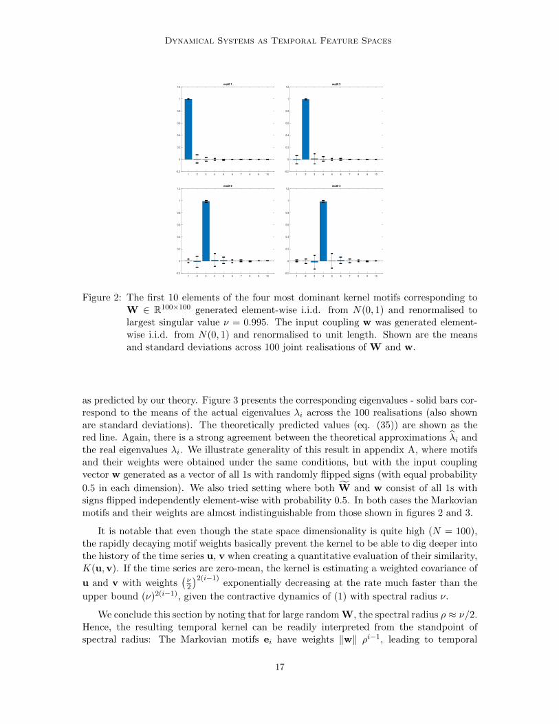
mal distribution N(0, 1). Each W was renormalised to W of largest singular value ν = 0.995and an input coupling vector w was generated as a random vector with elements generatedi.i.d. according to N(0, 1) and then renormalised to unit vector (length 1). We then imposeda past horizon τ = 200 and calculated the metric tensor Q, as well as its approximation Q(eq. (34)). In figure 2 we show the true motifs mi (eigenvectors of Q for the first four dom-inant motifs (motifs with the largest 4 motif weights) as the mean and standard deviationsacross the 100 realisations. For clarity, we only show the first 10 dimensions. It is clear thatthe motifs approximately correspond to the first four standard basis vectors ei, i = 1, 2, 3, 4,
16
Dynamical Systems as Temporal Feature Spaces
motif 1
1 2 3 4 5 6 7 8 9 10
-0.2
0
0.2
0.4
0.6
0.8
1
1.2
motif 2
1 2 3 4 5 6 7 8 9 10
-0.2
0
0.2
0.4
0.6
0.8
1
1.2
motif 3
1 2 3 4 5 6 7 8 9 10
-0.2
0
0.2
0.4
0.6
0.8
1
1.2
motif 4
1 2 3 4 5 6 7 8 9 10
-0.2
0
0.2
0.4
0.6
0.8
1
1.2
Figure 2: The first 10 elements of the four most dominant kernel motifs corresponding toW ∈ R100×100 generated element-wise i.i.d. from N(0, 1) and renormalised tolargest singular value ν = 0.995. The input coupling w was generated element-wise i.i.d. from N(0, 1) and renormalised to unit length. Shown are the meansand standard deviations across 100 joint realisations of W and w.
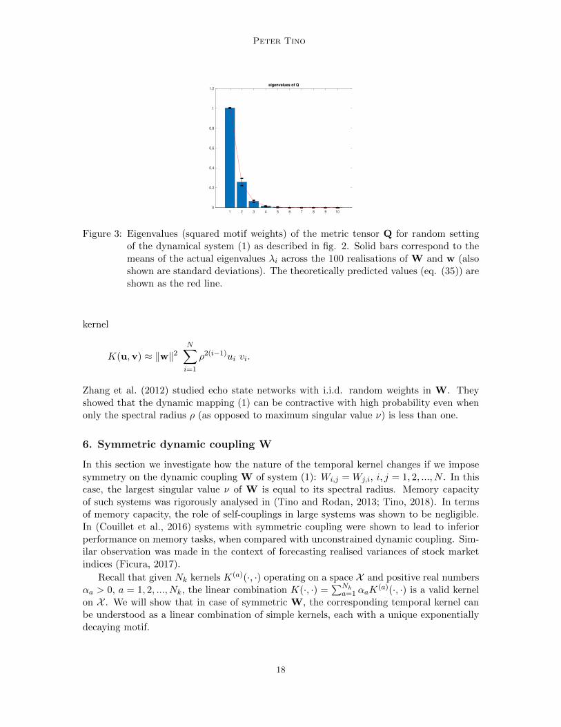
as predicted by our theory. Figure 3 presents the corresponding eigenvalues - solid bars cor-respond to the means of the actual eigenvalues λi across the 100 realisations (also shownare standard deviations). The theoretically predicted values (eq. (35)) are shown as thered line. Again, there is a strong agreement between the theoretical approximations λi andthe real eigenvalues λi. We illustrate generality of this result in appendix A, where motifsand their weights were obtained under the same conditions, but with the input couplingvector w generated as a vector of all 1s with randomly flipped signs (with equal probability
0.5 in each dimension). We also tried setting where both W and w consist of all 1s withsigns flipped independently element-wise with probability 0.5. In both cases the Markovianmotifs and their weights are almost indistinguishable from those shown in figures 2 and 3.
It is notable that even though the state space dimensionality is quite high (N = 100),the rapidly decaying motif weights basically prevent the kernel to be able to dig deeper intothe history of the time series u, v when creating a quantitative evaluation of their similarity,K(u,v). If the time series are zero-mean, the kernel is estimating a weighted covariance of
u and v with weights(ν2
)2(i−1)exponentially decreasing at the rate much faster than the
upper bound (ν)2(i−1), given the contractive dynamics of (1) with spectral radius ν.
We conclude this section by noting that for large random W, the spectral radius ρ ≈ ν/2.Hence, the resulting temporal kernel can be readily interpreted from the standpoint ofspectral radius: The Markovian motifs ei have weights ‖w‖ ρi−1, leading to temporal
17
Peter Tino
eigenvalues of Q
1 2 3 4 5 6 7 8 9 10
0
0.2
0.4
0.6
0.8
1
1.2
Figure 3: Eigenvalues (squared motif weights) of the metric tensor Q for random settingof the dynamical system (1) as described in fig. 2. Solid bars correspond to themeans of the actual eigenvalues λi across the 100 realisations of W and w (alsoshown are standard deviations). The theoretically predicted values (eq. (35)) areshown as the red line.
kernel
K(u,v) ≈ ‖w‖2N∑i=1
ρ2(i−1)ui vi.
Zhang et al. (2012) studied echo state networks with i.i.d. random weights in W. Theyshowed that the dynamic mapping (1) can be contractive with high probability even whenonly the spectral radius ρ (as opposed to maximum singular value ν) is less than one.
6. Symmetric dynamic coupling W
In this section we investigate how the nature of the temporal kernel changes if we imposesymmetry on the dynamic coupling W of system (1): Wi,j = Wj,i, i, j = 1, 2, ..., N . In thiscase, the largest singular value ν of W is equal to its spectral radius. Memory capacityof such systems was rigorously analysed in (Tino and Rodan, 2013; Tino, 2018). In termsof memory capacity, the role of self-couplings in large systems was shown to be negligible.In (Couillet et al., 2016) systems with symmetric coupling were shown to lead to inferiorperformance on memory tasks, when compared with unconstrained dynamic coupling. Sim-ilar observation was made in the context of forecasting realised variances of stock marketindices (Ficura, 2017).
Recall that given Nk kernels K(a)(·, ·) operating on a space X and positive real numbersαa > 0, a = 1, 2, ..., Nk, the linear combination K(·, ·) =
∑Nka=1 αaK
(a)(·, ·) is a valid kernelon X . We will show that in case of symmetric W, the corresponding temporal kernel canbe understood as a linear combination of simple kernels, each with a unique exponentiallydecaying motif.
18
Dynamical Systems as Temporal Feature Spaces
Theorem 3 Consider the dynamical system (1) of state dimensionality N with symmetriccoupling W of rank Nk ≤ N . Let s1, s2, ..., sNk
, be the eigenvectors of W corresponding tonon-zero eigenvalues σ1 ≥ σ2 ≥ ... ≥ σNk
. Denote by wa = s>a w the projection of the inputcoupling w onto the eigenvector sa. Then the temporal kernel K(·, ·) associated with system(1) is a linear combination of Nk kernels K(a)(·, ·),
K(·, ·) =
Nk∑a=1
w2a K
(a)(·, ·), (36)
each kernel K(a) with a single motif
m(a) = (1, σa, σ2a, ..., σ
τ−1a )> ∈ Rτ . (37)
Proof Since W is symmetric, it can be decomposed as
W = S Σ S>,
where S = [s1, s2, ..., sNk] is an N × Nk matrix storing the eigenvectors of W as columns,
with the associated eigenvalues organised along the diagonal of Σ = diag(σ1, σ2, ..., σNk).
The powers of W can be then expressed simply through powers of Σ: Wi = S Σi S>. Wethus have
Qi,j = w> (W>)i−1 Wj−1 w
= w> Wi+j−2 w (by symmetry of W)
= w>S Σi+j−2 S>w
= w> Σi+j−2 w, (38)
where w = S>w is the projection of input coupling w onto the orthonormal eigen-basis ofW.
Writing (38) as a quadratic form, we obtain
Qi,j =
Nk∑a,l=1
wa wl Σi+j−2a,l
=
Nk∑a=1
w2a σ
i+j−2a , (39)
because Σ is a diagonal matrix.Let us define Nk matrices Q(a) ∈ Rτ×τ , a = 1, 2, ..., Nk, as
Q(a)i,j = σi+j−2a .
Then,
Q =
Nk∑a=1
w2a Q(a). (40)
19
Peter Tino
Note that Q(a) are rank-1 positive semi-definite matrices Q(a) = m(a) (m(a))>. Since
Q(a) m(a) = m(a) (m(a))> m(a) = ‖m(a)‖22 m(a),
we have that m(a) is the only eigenvector of Q(a) with a non-zero eigenvalue, i.e. m(a) isthe only motif of the kernel
K(a)(u,v) = u> Q(a) v
with non-zero motif weight. From (40) it follows that K(u,v) =∑Nk
a=1 w2a K
(a)(u,v).
Theorem 3 states that the temporal kernel of a system (1) with symmetric couplingis a linear combination of several kernels, each of which corresponds to a single non-zeroeigenvalue σa of W. Each such kernel has a unique motif m(a) ∈ Rτ associated withit. The motifs m(a) can only be of two kinds: Either an exponentially decaying profile(1, σa, σ
2a, σ
3a, σ
4a, ...), if σa is positive, or an exponentially decaying profile with high oscilla-
tion frequency (1,−|σa|, σ2a,−|σ3a|, σ4a, ...), if σa is negative. This is obviously quite limiting,precluding the component kernels K(a)(·, ·) to capture more diverse range of possible dy-namic behaviours.
A word of caution is in order. The individual motifs m(a) are indeed motifs of thecomponent kernels K(a)(·, ·), but they are not motifs of the kernel K(·, ·). Even though onecan write
Q = V ΣW V>,
where the matrix V = [m(1),m(2), ...,m(Nk)] stores component motifs m(a) as columns andΣW = diag(w2
1, w2a, ..., w
2Nk
), the component motifs m(a) are not orthogonal. Hence, ingeneral there is no non-zero number κ, such that
Q m(a) = V ΣW V> m(a) = κ m(a).
Unlike in the previous section, because of the imposed symmetry on W, it is muchmore difficult to approximate the structure of Q. We can recover the upper bound (18) oftheorem 2 on absolute values of Qi,j . From Theorem 2 and eq. (39) we have
Qi,j =N∑a=1
w2a σ
i+j−2a
and
|Qi,j | ≤N∑a=1
w2a |σi+j−2a |
≤ νi+j−2a
N∑a=1
w2a (41)
≤ νi+j−2 ‖w‖22. (42)
Here (42) follows from (41) since the norm of the input coupling w is invariant with respectto orthonormal change of basis. The inequality in (42) becomes equality if W is full rank.
20
Dynamical Systems as Temporal Feature Spaces
7. W as a scaled permutation matrix
We will now consider a strongly constrained dynamical coupling W in the form of cyclicN ×N permutation matrix P, scaled by ν, so that the largest singular value, as well as thespectral radius of W = ν ·P is equal to ν. This follows from a theorem by Frobenius thatstates that for a non-negative matrix W, its spectral radius is lower and upper bounded bythe minimum and maximum row sum, respectively (e.g. (Minc, 1988)). Since in our caseall rows of W sum to ν, the spectral radius must be5 ν.
Without loss of generality6 we will consider cyclic permutation {1 → 2, 2 → 3, ..., N −1 → N,N → 1}, represented by Pi+1,i = 1, i = 1, 2, ..., N − 1 and P1,N = 1, all the otherelements of P are zero. Dynamic couplings in the form of scaled cyclic permutation matrixcorrespond to the setting of simple cycle reservoir (Rodan and Tino, 2011), where thereservoir units are connected in a uni-directional ring structure, with the same weight valueon all connections in the ring. Analogously, setting of the input coupling w can be verysimple, controlled again by a single amplitude value w > 0 for all input weights. Intuitively,all the input weights should not have the same value w, as this would greatly symmetrisethe ESN architecture. To break the symmetry, Rodan and Tino (2011) suggest to applyan a-periodic sign pattern to the input weights (e.g. according to binary expansion of anirrational number). While such a reservoir structure has the advantage of being extremelysimple and completely deterministic, the predictive performance of the associated ESNsin a variety of tasks on time series of different origins and memory structure was shownto be on par (and sometimes even better) with the usual random reservoir constructions(Rodan and Tino, 2011). Similar observations were made in (Strauss et al., 2012). This isof great practical importance, since many optics-based physical constructions of reservoirmodels follow the ring topology structure, which can be implemented using a single unitwith multiple delays (Rohm and Ludge, 2018; Tanaka et al., 2019; Appeltant et al., 2011).Yet, it has been unclear, why such a simple setting can be competitive in real word tasks, orwhy indeed the breaking of symmetry through a-periodic sign pattern in the input weightsis so crucial. In this section, we will study the nature of motifs associated with ring reservoirtopologies and the consequences of adopting periodic, rather than a-periodic input weightsign patterns.
Given a time horizon τ = `N , for some positive integer ` > 1, we will now show that thetemporal kernel motifs corresponding to the dynamical system (1) with scaled permutationcoupling W = ν ·P have an intricate block structure.
Theorem 4 Consider the dynamical system (1) of state space dimensionality N , with cou-pling W = ν · P, where ν ∈ (0, 1) and P is the N × N cyclic permutation matrix. Letmi ∈ RN , i = 1, 2, ..., N , be motifs of the temporal kernel associated with (1) under pasttime horizon equal to N . Denote the corresponding motif weights by ωi. Then, given adifferent past time horizon τ = ` · N , for some positive integer ` > 1, the temporal kernelmotifs mi ∈ Rτ associated with (1) have the following block form:
mi =(m>i , ν
Nm>i , ν2Nm>i , ..., ν
(`−1)Nm>i
)>, i = 1, 2, ...N.
5. Alternatively, this can be shown by arguing that W is a normal matrix.6. We can always renumber the state space dimensions.
21
Peter Tino
The corresponding motif weights are equal to
ωi = ωi
(1− ν2τ
1− ν2N
) 12
.
Proof Note that because P is a permutation matrix, for any non-negative integer i ∈ N0,we have
Pi = PN ·(i\N) Pi modN ,
where mod and \ denote the modulo and integer division operations. Since PN ·(i\N) =IN×N , we have Pi = PimodN . Consequently,
Wi = νi ·Pi modN .
Furthermore, since P is orthogonal, P−1 = P>. We can now write the elements of Q as(see eq. (17)),
Qi,j = w> (W>)i−1 Wj−1 w
= νi+j−2 w> (P>)i−1 Pj−1 w
= νi+j−2 w> Pj−i w.
= νi+j−2 w> P(j−i) modN w. (43)
For k ∈ {−N + 1,−N + 2, ...,−1, 0, 1, ...N − 1}, if k is positive, Pkw is the vector withelements of w rotated k places to the right. In case k is negative, the rotation is to the left.From (43) it is clear the Q ∈ Rτ×τ has the following block structure:
Q =
Q(1,1) Q(1,2) · · · Q(1,`)
Q(2,1) Q(2,2) · · · Q(2,`)
· · · · · · · · · · · ·Q(`,1) Q(`,2) · · · Q(`,`)
,where each matrix Q(a,b) ∈ RN×N , a, b = 1, 2, .., , `, has elements
Q(a,b)i,j = ν(a+b−2)N νi+j−2 w> Pj−i w, i, j = 1, 2, ..., N.
Define an N ×N matrix R with elements
Ri,j = νi+j−2 w> Pj−i w, i, j = 1, 2, ..., N, (44)
yielding Q(a,b) = ν(a+b−2)N R. Note that R is the metric tensor of the temporal kernelassociated with (1) under the past time horizon N . Let mi ∈ RN be the i-th eigenvector ofR with eigenvalue λi. Then,
Q(a,b) mi = ν(a+b−2)N λi mi,
22
Dynamical Systems as Temporal Feature Spaces
and so
[Q(a,1),Q(a,2), · · · ,Q(a,`)
]mi
mi
· · ·mi
= λi
∑j=1
ν(j−1)N
ν(a−1)N mi. (45)
It follows that for each a ∈ {1, 2, ..., `},
[Q(a,1),Q(a,2), · · · ,Q(a,`)
]mi
νN mi
· · ·ν(`−1)N mi
= λi
∑j=1
ν2(j−1)N
ν(a−1)N mi. (46)
We can thus conclude that the vector
mi =(m>i , ν
Nm>i , ν2Nm>i , ..., ν
(`−1)Nm>i
)>is an eigenvector of Q with eigenvalue
λi = λi
`−1∑j=0
(ν2N
)j= λi
1− ν2N`
1− ν2N.
= λi1− ν2τ
1− ν2N.
7.1. Periodic input coupling w
It has been empirically shown in (Rodan and Tino, 2011) that when the dynamic couplingW is formed by a scaled permutation matrix, a very simple setting of input coupling wis sufficient: all elements of w can have the same absolute value, but the sign patternshould be aperiodic. Intuitively, it is clear that for such W a periodic input coupling w willinduce symmetry in the dynamic processing of (1) and such a symmetry should be broken.However, in this section we would like to ask exactly what representational capabilities arelost by imposing a periodicity in w.
We will start by considering a general case of periodic w ∈ RN formed by k > 1 copiesof a periodic block s ∈ Rp, w = (s>, s>, ..., s>)>. Obviously, N = k · p.
Denote by P ∈ Rp×p the top left p × p block of the right shift permutation matrixP ∈ RN×N . In other words, P is the right shift permutation matrix operating on vectorsfrom Rp. Furthermore, we introduce matrix T ∈ Rp×p with elements
Ti,j = νi+j−2⟨s,P
|j−i|s⟩, i, j = 1, 2, ..., p. (47)
23
Peter Tino
Theorem 5 Consider the dynamical system (1) of state space dimensionality N , with cou-pling W = ν · P, where ν ∈ (0, 1) and P is the N × N cyclic permutation matrix. Letthe input coupling w ∈ RN consist of k > 1 copies of a periodic block s ∈ Rp. Denote bymi ∈ Rp, i = 1, 2, ..., p, eigenvectors of the matrix T (47) with the corresponding eigenval-ues λi. Then, given a past time horizon τ = ` · N , for some positive integer ` > 1, thereare at most p temporal kernel motifs mi ∈ Rτ associated with (1) of non-zero motif weight.Furthermore, the kernel motifs have the following block form,
mi = (m>i , νp m>i , ν
2p m>i , ..., ντ−p m>i )>, i = 1, 2, ...p,
with the corresponding motif weights
ωi =
(λi
1− ν2τ
1− ν2p
) 12
.
Proof By Theorem 4, to determine motifs of the temporal kernel associated with (1), it issufficient to perform eigen-analysis of the block matrix Q(1,1) = R (eq. (44)).
For a = 0, 1, 2, ..., N − 1,
〈w,Paw〉 = k ·⟨s,P
as⟩
= k ·⟨s,P
a mod ps⟩
and since R is symmetric, from (eq. (44)) we have
Q(1,1)i,j = k · νi+j−2 ·
⟨s,P
|j−i| mod ps⟩, i, j = 1, 2, ..., N. (48)
Therefore, Q(1,1) can be decomposed into blocks of p× p matrices
Q(1,1) =
C(1,1) C(1,2) · · · C(1,k)
C(2,1) C(2,2) · · · C(2,k)
· · · · · · · · · · · ·Ck,1) C(k,2) · · · C(k,k)
,where
C(c,d) = ν(c+d−2)p C(1,1), c, d = 1, 2, ..., k
and
C(1,1)i,j = νi+j−2 ·
⟨s,P
|j−i|s⟩, i, j = 1, 2, ..., p.
Now, let mi ∈ Rp be the i-th eigenvector of C(1,1) = T with eigenvalue λi. Then,
C(c,d) mi = ν(c+d−2)p C(1,1) mi = ν(c+d−2)p λi mi.
We have
[C(c,1),C(c,2), · · · ,C(c,k)
]mi
νp mi
· · ·ν(k−1)p mi
= λi
k∑j=1
ν2(j−1)p
ν(c−1)p mi (49)
24
Dynamical Systems as Temporal Feature Spaces
for c = 1, 2, ..., k. Hence,
mi = (m>i , νp m>i , ν
2p m>i , ..., ν(k−1)p m>i )>
is an eigenvector of Q(1,1) with eigenvalue
λi = λi
k−1∑j=0
(ν2p)j
= λi1− ν2pk
1− ν2p.
= λi1− ν2N
1− ν2p.
By Theorem 4, the corresponding eigenvector mi of Q reads:
mi = (m>i , νNm>i , ..., ν
(`−1)Nm>i )>
= (m>i , νp m>i , ..., ν
(k−1)p m>i , νN m>i , ν
N+p m>i , ..., ν(`−1)N+(k−1)p m>i )>
= (m>i , νp m>i , ν
2p ..., ντ−p m>i )>.
The last equality holds since from τ = `N and N = kp, we have (`−1)N +(k−1)p = τ −p.We can calculate the corresponding eigenvalue as
λi = λi1− ν2τ
1− ν2N
= λi1− ν2N
1− ν2p1− ν2τ
1− ν2N= λi
1− ν2τ
1− ν2p.
Theorem 5 formally specifies consequences for the dynamical kernel of having a periodicinput coupling w of period p in the system (1). First, the number of potentially usefulkernel motifs of non-zero weight is reduced from N (the state space dimensionality) to p.Second, the motif structure is even more restricted than in the case of general w. If thepast horizon is τ = `N , then in general, by theorem 4, each motif mi ∈ Rτ consists of aseries of ` copies of the same “core motif” mi ∈ RN , down-weighted by exponential decay.In the case of periodic w, motifs mi ∈ Rτ are formed by a series of `k copies of the samesmall block mi ∈ Rp, down-weighted by exponential decay.
We will now investigate special settings of the periodic input coupling w ∈ RN . Considerfirst the binary setting, i.e. the core periodic block is s = (1, 0, 0, ..., 0)> ∈ {0, 1}p. Assumew contains k such blocks (N = k · p). Then, since for a = 0, 1, 2, ..., p− 1,
⟨s,P
as⟩
=
{1, if a = 00, otherwise,
the matrix T ∈ Rp×p (eq. (47)) will have a diagonal form, T = diag(1, ν2, ..., ν2(p−1)). Theeigenvectors mi ∈ Rp of T, i = 1, 2, ..., p, correspond to the standard basis ei of Rp, i.e.
25

Peter Tino
all elements of ei are zeros, except for the i-th element, which is 1. The correspondingeigenvalues are λi = ν2(i−1). By theorem 5, each motif
mi = (e>i , νp e>i , ν
2p e>i , ..., ντ−p e>i )>, (50)
with motif weight
ωi = νi−1(
1− ν2τ
1− ν2p
) 12
. (51)
is a periodic exponentially decaying motif that picks up elements of time series driving (1)with periodicity p and initial lag i. Given a time series u ∈ Rτ ,
〈mi,u〉 =`·k∑j=1
ν(j−1)p ui+(j−1)p.
In the representation of (eq. (21)) we then have
u =
(1− ν2τ
1− ν2p
) 12
· (〈m1,u〉 , ν 〈m2,u〉 , ..., νp−1 〈mp,u〉)> ∈ Rp.
Given another time series v ∈ Rτ , the temporal kernel gives
K(u,v) = 〈u, v〉
=1− ν2τ
1− ν2pp∑i=1
ν2(i−1) 〈mi,u〉 〈mi,v〉 . (52)
In the case of all-ones w with a periodic sign pattern, the core periodic block is s =(+1,−1,−1, ...,−1)> ∈ {−1,+1}p. For a = 0, 1, 2, ..., p− 1, we have
⟨s,P
as⟩
=
{p, if a = 0p− 4, otherwise,
From (eq. (47)), the matrix T ∈ Rp×p with elements
Ti,j =
{ν2(i−1) p, if i = jνi+j−2 (p− 4), otherwise,
can yield a richer set of eigenvectors mi than the standard basis ei in Rp. An exceptionis the case of period-4 sign pattern, p = 4. In that case, T is a diagonal matrix T =p · diag(1, ν2, ..., ν2(p−1)), exactly the scaled version of T analysed above, when w was thebinary vector composed of a series of k blocks of e1 ∈ Rp. Hence the four motifs mi willhave the form suggested by eq. (50) and the motif weights (51) will be scaled by
√p = 2.
We have thus established:
26
Dynamical Systems as Temporal Feature Spaces
Corollary 6 Under the assumptions of Theorem 5, assume that the input coupling w ∈{0, 1}N consists of k > 1 copies of the binary standard basis block s = e1 ∈ {0, 1}p. Thenthere are p non-zero wight motifs of the dynamic kernel associated with (1),
mi = (e>i , νp e>i , ν
2p e>i , ..., ντ−p e>i )>,
with motif weights
ωi = νi−1(
1− ν2τ
1− ν2p
) 12
.
Each mi is thus a periodic exponentially decaying motif that picks up elements of input timeseries with periodicity p and initial lag i.
Furthermore, if the bipolar input coupling w ∈ {−1,+1}N consists of k > 1 copies ofthe block s = 2e1−1 ∈ {−1,+1}4 of period p = 4, then there are four non-zero wight motifsmi (50) with motif weights 2ωi.
8. Illustrative examples
In this section we will illustrate the results obtained so far showing the influence of thedynamic and input coupling, W and w, respectively, on the strength and richness of motifsof the temporal kernel associated with the dynamical system (1). In all illustrations wewill use state space dimensionality N = 100 and re-normalise the dynamic coupling W ∈R100×100 to largest singular value ν = 0.995. The input coupling w is renormalized to unitlength. The past horizon will be set to τ = 200. We will show motifs with motif weightsup to 10−2 of the highest motif weight.
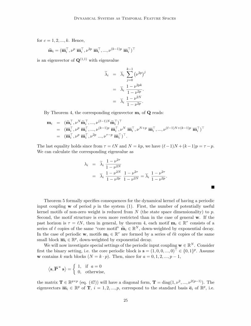
Figure 4 (left) shows motifs of the temporal kernel given by random coupling W, whereall elements Wi,j were generated i.i.d. from normal distribution N(0, 1). The motifs areshown in a column-wise fashion, i.e. the x-axis indexes the individual motifs, while themotif values are shown along the y-axis. The associated motif weights are presented in theright plot.
As explained in section 5, each of the Markovian motifs picks an element from the recenttime series history, yielding a shallow memory involved in the kernel evaluation, with rapidlydecaying motif weights. Almost identical results were obtained for Wi,j and wi generatedi.i.d. from other distributions (e.g. uniform over [−1,+1], Bernoulli over {−1,+1} or{0, 1}), as well as for many other settings of w, including the all-ones vector w = 1.
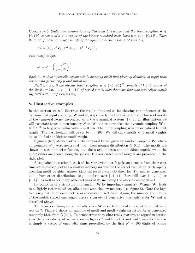
Introduction of a structure into random W by imposing symmetry (Wigner W) leadsto a slightly richer motif set, albeit still with shallow memory (see figure 5). Note the highfrequency nature of some motifs, as discussed in section 6. Again, the number and natureof the motifs stayed unchanged across a variety of generative mechanisms for W and wdescribed above.
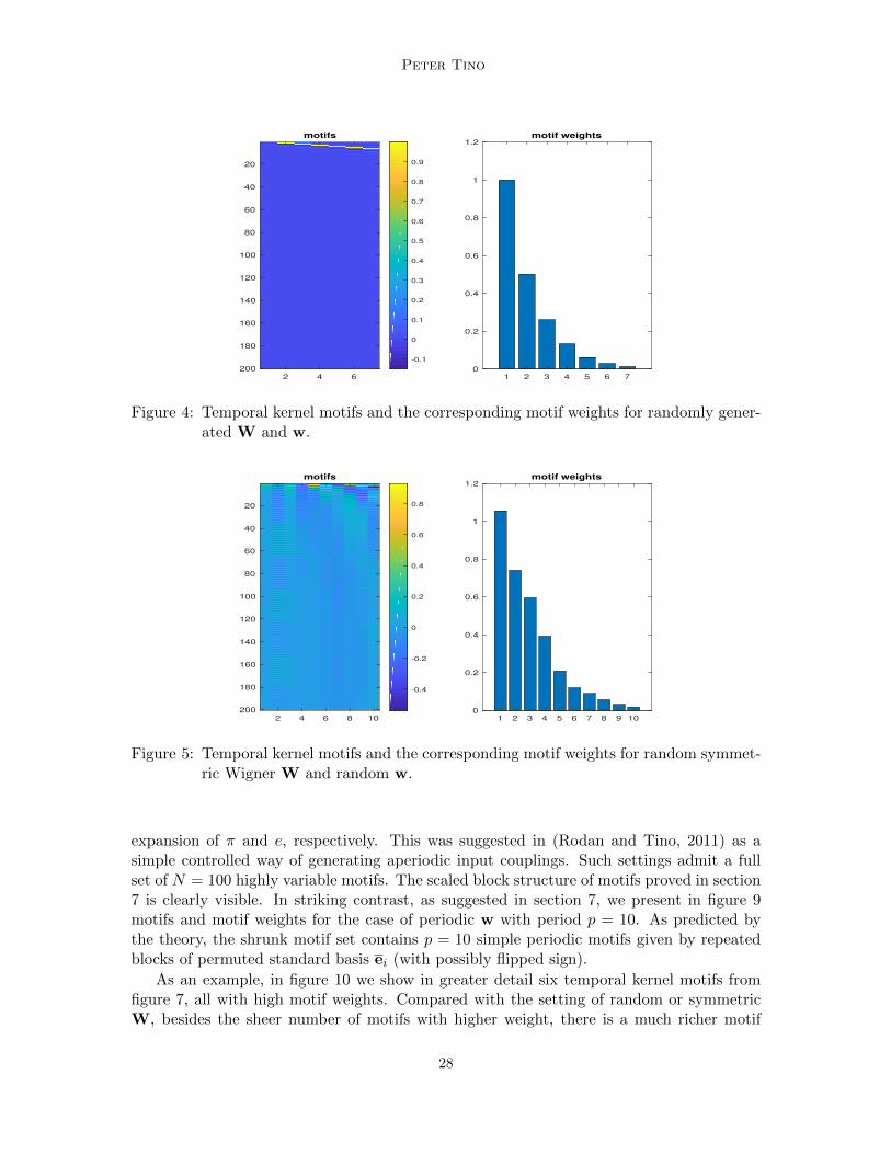
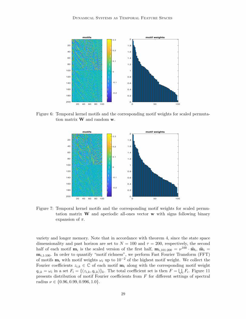
The situation changes dramatically when W is set to the scaled permutation matrix ofsection 7. Figure 6 shows an example of motif and motif weight structure for w generatedrandomly i.i.d. from N(0, 1). To demonstrate that what really matters, as argued in section7, is the aperiodicity of w, we show in figures 7 and 8 motifs and motif weights when wis simply a vector of ones with signs prescribed by the first N = 100 digits of binary
27
Peter Tino
motifs
2 4 6
20
40
60
80
100
120
140
160
180
200
-0.1
0
0.1
0.2
0.3
0.4
0.5
0.6
0.7
0.8
0.9
motif weights
1 2 3 4 5 6 7
0
0.2
0.4
0.6
0.8
1
1.2
Figure 4: Temporal kernel motifs and the corresponding motif weights for randomly gener-ated W and w.
motifs
2 4 6 8 10
20
40
60
80
100
120
140
160
180
200
-0.4
-0.2
0
0.2
0.4
0.6
0.8
motif weights
1 2 3 4 5 6 7 8 9 10
0
0.2
0.4
0.6
0.8
1
1.2
Figure 5: Temporal kernel motifs and the corresponding motif weights for random symmet-ric Wigner W and random w.
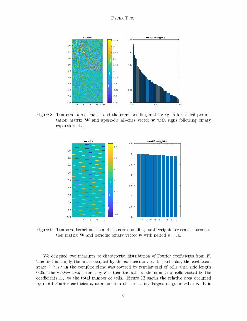
expansion of π and e, respectively. This was suggested in (Rodan and Tino, 2011) as asimple controlled way of generating aperiodic input couplings. Such settings admit a fullset of N = 100 highly variable motifs. The scaled block structure of motifs proved in section7 is clearly visible. In striking contrast, as suggested in section 7, we present in figure 9motifs and motif weights for the case of periodic w with period p = 10. As predicted bythe theory, the shrunk motif set contains p = 10 simple periodic motifs given by repeatedblocks of permuted standard basis ei (with possibly flipped sign).
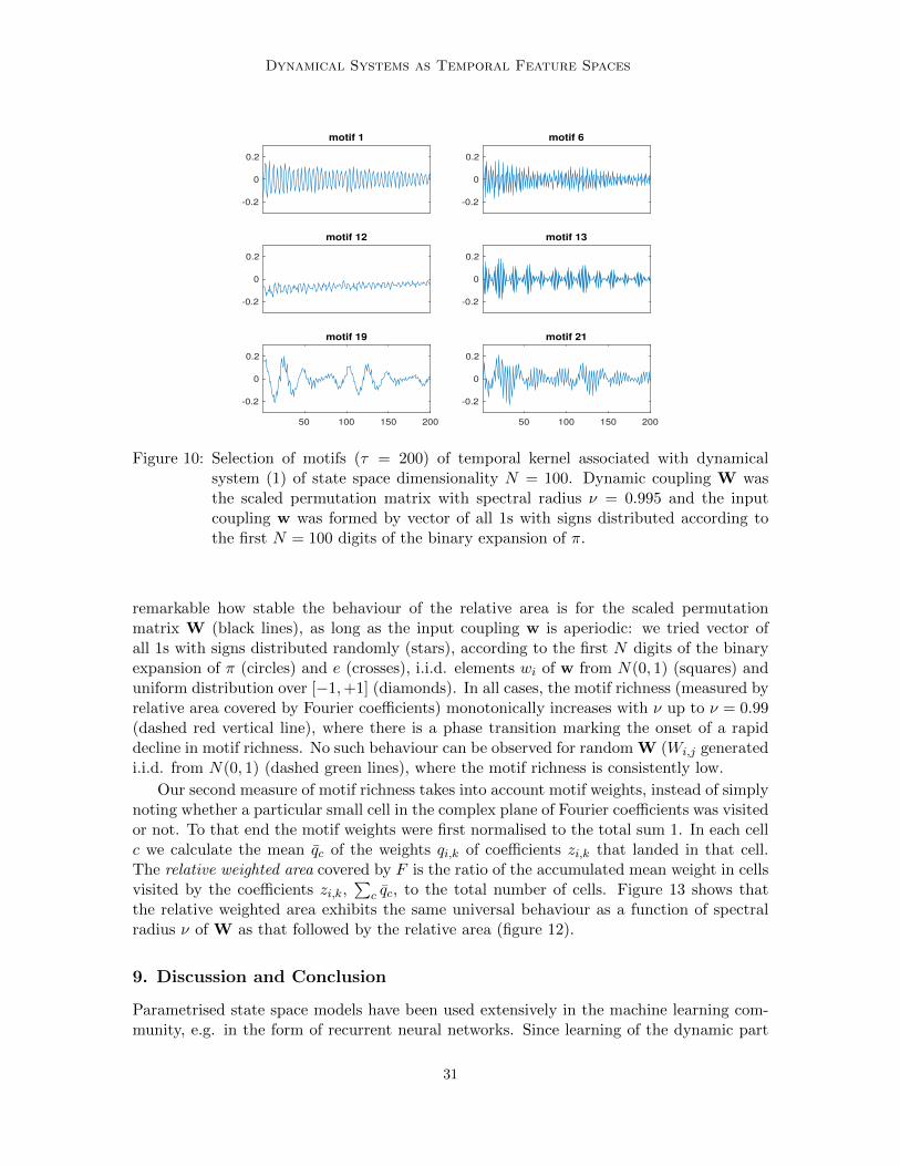
As an example, in figure 10 we show in greater detail six temporal kernel motifs fromfigure 7, all with high motif weights. Compared with the setting of random or symmetricW, besides the sheer number of motifs with higher weight, there is a much richer motif
28
Dynamical Systems as Temporal Feature Spaces
motifs
20 40 60 80 100
20
40
60
80
100
120
140
160
180
200
-0.2
-0.1
0
0.1
0.2
0.3
motif weights
0 50 100
0
0.2
0.4
0.6
0.8
1
1.2
1.4
1.6
1.8
2
Figure 6: Temporal kernel motifs and the corresponding motif weights for scaled permuta-tion matrix W and random w.
motifs
20 40 60 80 100
20
40
60
80
100
120
140
160
180
200
-0.2
-0.1
0
0.1
0.2
0.3
motif weights
0 50 100
0
0.2
0.4
0.6
0.8
1
1.2
1.4
1.6
1.8
2
Figure 7: Temporal kernel motifs and the corresponding motif weights for scaled permu-tation matrix W and aperiodic all-ones vector w with signs following binaryexpansion of π.
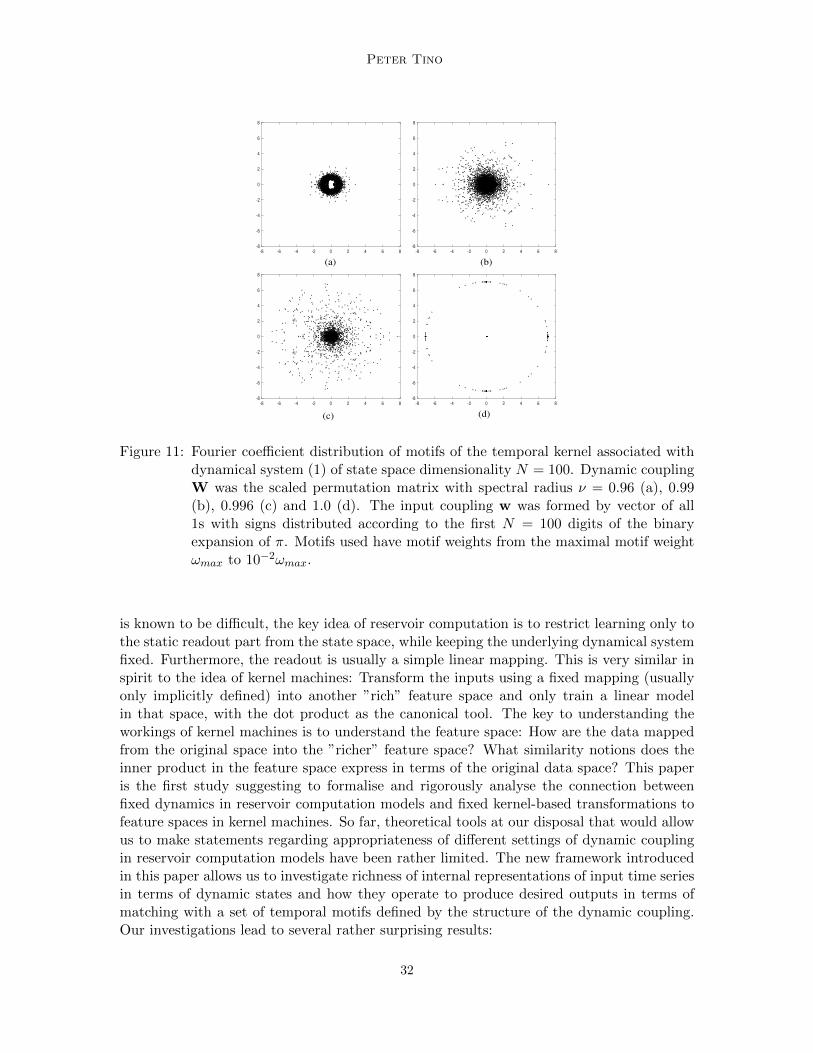
variety and longer memory. Note that in accordance with theorem 4, since the state spacedimensionality and past horizon are set to N = 100 and τ = 200, respectively, the secondhalf of each motif mi is the scaled version of the first half, mi,101:200 = ν100 · mi, mi =mi,1:100. In order to quantify “motif richness”, we perform Fast Fourier Transform (FFT)of motifs mi with motif weights ωi up to 10−2 of the highest motif weight. We collect theFourier coefficients zi,k ∈ C of each motif mi along with the corresponding motif weightqi,k = ωi in a set Fi = {(zi,k, qi,k)}k. The total coefficient set is then F =
⋃i Fi. Figure 11
presents distribution of motif Fourier coefficients from F for different settings of spectralradius ν ∈ {0.96, 0.99, 0.996, 1.0}.
29
Peter Tino
motifs
20 40 60 80 100
20
40
60
80
100
120
140
160
180
200 -0.25
-0.2
-0.15
-0.1
-0.05
0
0.05
0.1
0.15
0.2
0.25
motif weights
0 50 100
0
0.5
1
1.5
2
2.5
Figure 8: Temporal kernel motifs and the corresponding motif weights for scaled permu-tation matrix W and aperiodic all-ones vector w with signs following binaryexpansion of e.
motifs
2 4 6 8 10
20
40
60
80
100
120
140
160
180
200
-0.3
-0.2
-0.1
0
0.1
0.2
0.3
motif weights
1 2 3 4 5 6 7 8 9 10
0
0.5
1
1.5
2
2.5
3
3.5
Figure 9: Temporal kernel motifs and the corresponding motif weights for scaled permuta-tion matrix W and periodic binary vector w with period p = 10.
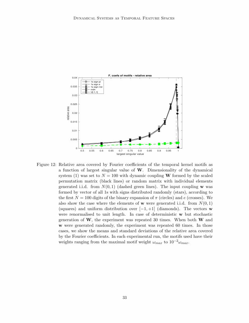
We designed two measures to characterise distribution of Fourier coefficients from F .The first is simply the area occupied by the coefficients zi,k. In particular, the coefficientspace [−7, 7]2 in the complex plane was covered by regular grid of cells with side length0.05. The relative area covered by F is then the ratio of the number of cells visited by thecoefficients zi,k to the total number of cells. Figure 12 shows the relative area occupiedby motif Fourier coefficients, as a function of the scaling largest singular value ν. It is
30
Dynamical Systems as Temporal Feature Spaces
-0.2
0
0.2
motif 1
-0.2
0
0.2
motif 6
-0.2
0
0.2
motif 12
-0.2
0
0.2
motif 13
50 100 150 200
-0.2
0
0.2
motif 19
50 100 150 200
-0.2
0
0.2
motif 21
Figure 10: Selection of motifs (τ = 200) of temporal kernel associated with dynamicalsystem (1) of state space dimensionality N = 100. Dynamic coupling W wasthe scaled permutation matrix with spectral radius ν = 0.995 and the inputcoupling w was formed by vector of all 1s with signs distributed according tothe first N = 100 digits of the binary expansion of π.
remarkable how stable the behaviour of the relative area is for the scaled permutationmatrix W (black lines), as long as the input coupling w is aperiodic: we tried vector ofall 1s with signs distributed randomly (stars), according to the first N digits of the binaryexpansion of π (circles) and e (crosses), i.i.d. elements wi of w from N(0, 1) (squares) anduniform distribution over [−1,+1] (diamonds). In all cases, the motif richness (measured byrelative area covered by Fourier coefficients) monotonically increases with ν up to ν = 0.99(dashed red vertical line), where there is a phase transition marking the onset of a rapiddecline in motif richness. No such behaviour can be observed for random W (Wi,j generatedi.i.d. from N(0, 1) (dashed green lines), where the motif richness is consistently low.
Our second measure of motif richness takes into account motif weights, instead of simplynoting whether a particular small cell in the complex plane of Fourier coefficients was visitedor not. To that end the motif weights were first normalised to the total sum 1. In each cellc we calculate the mean qc of the weights qi,k of coefficients zi,k that landed in that cell.The relative weighted area covered by F is the ratio of the accumulated mean weight in cellsvisited by the coefficients zi,k,
∑c qc, to the total number of cells. Figure 13 shows that
the relative weighted area exhibits the same universal behaviour as a function of spectralradius ν of W as that followed by the relative area (figure 12).
9. Discussion and Conclusion
Parametrised state space models have been used extensively in the machine learning com-munity, e.g. in the form of recurrent neural networks. Since learning of the dynamic part
31
Peter Tino
-8 -6 -4 -2 0 2 4 6 8
-8
-6
-4
-2
0
2
4
6
8
-8 -6 -4 -2 0 2 4 6 8
-8
-6
-4
-2
0
2
4
6
8
-8 -6 -4 -2 0 2 4 6 8
-8
-6
-4
-2
0
2
4
6
8
-8 -6 -4 -2 0 2 4 6 8
-8
-6
-4
-2
0
2
4
6
8
(a) (b)
(c) (d)
Figure 11: Fourier coefficient distribution of motifs of the temporal kernel associated withdynamical system (1) of state space dimensionality N = 100. Dynamic couplingW was the scaled permutation matrix with spectral radius ν = 0.96 (a), 0.99(b), 0.996 (c) and 1.0 (d). The input coupling w was formed by vector of all1s with signs distributed according to the first N = 100 digits of the binaryexpansion of π. Motifs used have motif weights from the maximal motif weightωmax to 10−2ωmax.
is known to be difficult, the key idea of reservoir computation is to restrict learning only tothe static readout part from the state space, while keeping the underlying dynamical systemfixed. Furthermore, the readout is usually a simple linear mapping. This is very similar inspirit to the idea of kernel machines: Transform the inputs using a fixed mapping (usuallyonly implicitly defined) into another ”rich” feature space and only train a linear modelin that space, with the dot product as the canonical tool. The key to understanding theworkings of kernel machines is to understand the feature space: How are the data mappedfrom the original space into the ”richer” feature space? What similarity notions does theinner product in the feature space express in terms of the original data space? This paperis the first study suggesting to formalise and rigorously analyse the connection betweenfixed dynamics in reservoir computation models and fixed kernel-based transformations tofeature spaces in kernel machines. So far, theoretical tools at our disposal that would allowus to make statements regarding appropriateness of different settings of dynamic couplingin reservoir computation models have been rather limited. The new framework introducedin this paper allows us to investigate richness of internal representations of input time seriesin terms of dynamic states and how they operate to produce desired outputs in terms ofmatching with a set of temporal motifs defined by the structure of the dynamic coupling.Our investigations lead to several rather surprising results:
32
Dynamical Systems as Temporal Feature Spaces
0.5 0.55 0.6 0.65 0.7 0.75 0.8 0.85 0.9 0.95 1
largest singular value
0
0.005
0.01
0.015
0.02
0.025
0.03
0.035
0.04
rela
tive
are
a
F. coefs of motifs - relative area
1s sign pi
1s sign e
1s sign rnd
rndn
U[-1,1]
Figure 12: Relative area covered by Fourier coefficients of the temporal kernel motifs asa function of largest singular value of W. Dimensionality of the dynamicalsystem (1) was set to N = 100 with dynamic coupling W formed by the scaledpermutation matrix (black lines) or random matrix with individual elementsgenerated i.i.d. from N(0, 1) (dashed green lines). The input coupling w wasformed by vector of all 1s with signs distributed randomly (stars), according tothe first N = 100 digits of the binary expansion of π (circles) and e (crosses). Wealso show the case where the elements of w were generated i.i.d. from N(0, 1)(squares) and uniform distribution over [−1,+1] (diamonds). The vectors wwere renormalised to unit length. In case of deterministic w but stochasticgeneration of W, the experiment was repeated 30 times. When both W andw were generated randomly, the experiment was repeated 60 times. In thosecases, we show the means and standard deviations of the relative area coveredby the Fourier coefficients. In each experimental run, the motifs used have theirweights ranging from the maximal motif weight ωmax to 10−2ωmax.
33
Peter Tino
0.5 0.55 0.6 0.65 0.7 0.75 0.8 0.85 0.9 0.95 1
largest singular value
0
0.002
0.004
0.006
0.008
0.01
0.012
0.014
0.016
0.018
rela
tive
are
a
F. coefs - relative area (mean m. weight)
1s sign pi
1s sign e
1s sign rnd
rndn
U[-1,1]
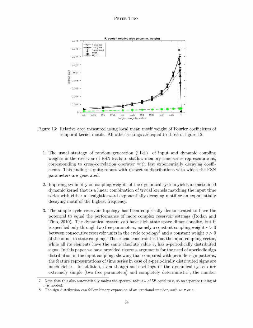
Figure 13: Relative area measured using local mean motif weight of Fourier coefficients oftemporal kernel motifs. All other settings are equal to those of figure 12.
1. The usual strategy of random generation (i.i.d.) of input and dynamic couplingweights in the reservoir of ESN leads to shallow memory time series representations,corresponding to cross-correlation operator with fast exponentially decaying coeffi-cients. This finding is quite robust with respect to distributions with which the ESNparameters are generated.
2. Imposing symmetry on coupling weights of the dynamical system yields a constraineddynamic kernel that is a linear combination of trivial kernels matching the input timeseries with either a straightforward exponentially decaying motif or an exponentiallydecaying motif of the highest frequency.
3. The simple cycle reservoir topology has been empirically demonstrated to have thepotential to equal the performance of more complex reservoir settings (Rodan andTino, 2010). The dynamical system can have high state space dimensionality, but itis specified only through two free parameters, namely a constant coupling weight r > 0between consecutive reservoir units in the cycle topology7 and a constant weight v > 0of the input-to-state coupling. The crucial constraint is that the input coupling vector,while all its elements have the same absolute value v, has a-periodically distributedsigns. In this paper we have provided rigorous arguments for the need of aperiodic signdistribution in the input coupling, showing that compared with periodic sign patterns,the feature representations of time series in case of a-periodically distributed signs aremuch richer. In addition, even though such settings of the dynamical system areextremely simple (two free parameters) and completely deterministic8, the number
7. Note that this also automatically makes the spectral radius ν of W equal to r, so no separate tuning ofν is needed.
8. The sign distribution can follow binary expansion of an irrational number, such as π or e.
34
Dynamical Systems as Temporal Feature Spaces
and variety of dynamic motifs of the associated dynamic kernel are far superior to thestandard configurations of ESN that rely on stochastic generation of coupling weights.
4. By quantifying motif richness of the dynamic kernel associated with cycle reservoirtopology, we showed that there is a phase transition in motif richness at spectral radiusvalues close to, but strictly less than 1. This confirms previous findings in the ESNliterature on the importance of tuning the dynamical system at the edge of stability(Bertschinger and Natschlger, 2004).
The arguments in this paper were developed under the assumption of linear dynamicalsystem with linear readout map. However, it has been proved that even linear dynamicalsystems can be universal, provided they are equipped with polynomial readout maps (Grig-oryeva and Ortega, 2018b,a; Gonon and Ortega, 2019). In our setting, this corresponds toconsidering instead of the linear kernel (eq. (16)) a polynomial kernel (of some degree d),
K(u,v) = (〈φ(u), φ(v)〉+ a)d. (53)
Clearly, memory characteristics of such a kernel will not change with offset a ∈ R orincreasing polynomial degree d. By eqs. (20-21), the polynomial kernel can be written as
K(u,v) = (〈u, v〉+ a)d, (54)
where the elements ui, vi, i = 1, 2, ..., Nm, of u, v ∈ RNm are projections of u,v ∈ Rτonto motifs mi ∈ Rτ , scaled by the motif weight. Non-linear manipulation of ui, vi canincrease the capacity of the readout mapping but only at the level of memory and featureset defined by the motifs. Randomly generated or symmetric reservoir couplings will stilllead to constrained shallow memory kernels. We have shown that simple cycle reservoirstuned at the edge of stability, with aperiodic sign patterns in input coupling are among theESN architectures capable of approximating deep memory processes when linear dynamicalsystem and polynomial readout are used. Of course, when non-linearity is allowed in thedynamical system (for example, by employing a logistic sigmoid transfer function), evenrandomly generated reservoirs may be able to capture deeper memory.
Our study contributes to the debate about what characteristics of the dynamical systemare desirable to make it a ‘universal’ temporal filter capable of producing rich representationsof input time series in its state space. Such representations can then be further utilisedby readouts, purpose-build for a variety tasks. Ozturk et al. (2007) hypothesised thatthe distribution of reservoir activations should have high entropy and suggested that itwas desirable for the reservoir weight matrix to have eigenvalues uniformly distributedinside the unit circle. In this way the system dynamics would include uniform coverageof time constants (related to the uniform distribution of the poles) (Ozturk et al., 2007).Our work suggests a counterargument when linear reservoirs and non-linear readouts areused: Uniform distribution of eigenvalues inside the unit circle can be achieved by randomgeneration of the reservoir matrix. However, this leads to a highly constrained set of shallowmemory motifs of the associated dynamic kernel that describes how features of time seriesseen in the past contribute to the production of the model output. On the other hand, a verysimple setting of high dimensional dynamical system governed by just two free parameterscan achieve a much richer and deeper memory motifs of the dynamic kernel. Note that in
35
Peter Tino
this case, the eigenvalues of the reservoir coupling matrix are distributed uniformly along acircle with radius equal to the spectral radius of the reservoir matrix.
Acknowledgement:This work was supported by the European Commission Horizon 2020 Innovative TrainingNetwork SUNDIAL (SUrvey Network for Deep Imaging Analysis and Learning), ProjectID: 721463.
Appendix A. Markovian motifs resulting from random dynamicalcoupling W
In this appendix we demonstrate that the approximations in section 5 of motifs and theirweights in the case of random dynamic coupling W hold for diverse distributions used togenerate elements of W. In particular, in figure 14 we show kernel motifs obtained from W ∈R100×100 generated element-wise i.i.d. from N(0, 1) and renormalised to largest singularvalue ν = 0.995 (the setting used in section 5) and input coupling vector w generated as avector of all 1s with randomly flipped signs (in each dimension with equal probability 0.5),renormalised to unit vector. The associated squared motif weights are presented in figure15. We also show in figures 16 and 17 the kernel motifs and eigenvalues of Q when both Wand w consist of all 1s with signs flipped independently element-wise with probability 0.5(dynamical coupling renormalised to largest singular value ν = 0.995 and w to unit vector).In both cases, the Markovian motifs and their weights are almost indistinguishable fromthose shown in section 5 (figures 2 and 3).
References
L. Appeltant, M. C. Soriano, G. Van der Sande, J. Danckaert, S. Massar, J. Dambre,B. Schrauwen, C. R. Mirasso, and I. Fischer. Information processing using a singledynamical node as complex system. Nature Comm., 2, 2011.
L. E. Baum and T. Petrie. Statistical inference for probabilistic functions of finite statemarkov chains. Ann. Math. Statist., 37(6):1554–1563, 12 1966.
Y. Bengio, P. Frasconi, and P Simard. The problem of learning long-term dependencies inrecurrent networks. In Proceedings of the 1993 IEEE International Conference on NeuralNetworks, volume 3, pages 1183–1188, 1993.
Y. Bengio, P. Simard, and P. Frasconi. Learning long-term dependencies with gradientdescent is difficult. IEEE Transactions on Neural Networks, 5(2):157–166, 1994.
Nils Bertschinger and Thomas Natschlger. Real-time computation at the edge of chaos inrecurrent neural networks. Neural Computation, 16(7):1413–1436, 2004.
Terry Bossomaier, Lionel Barnett, Michael Harr, and Joseph T. Lizier. An Introduction toTransfer Entropy: Information Flow in Complex Systems. Springer Publishing Company,Incorporated, 1st edition, 2016.
36
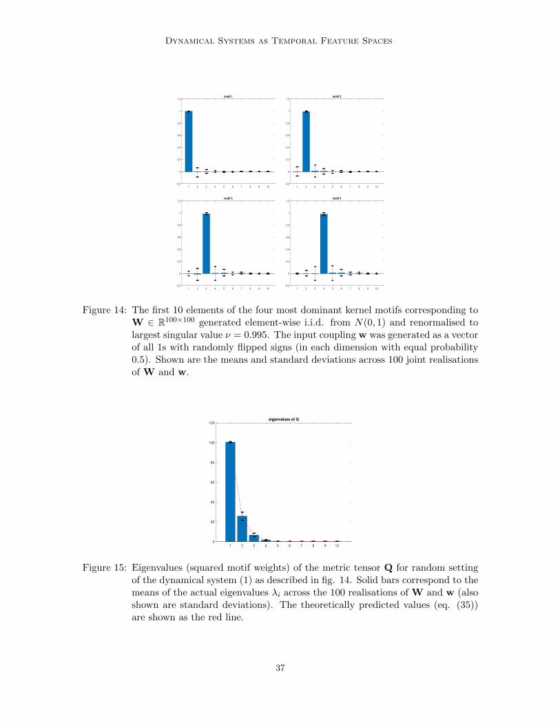
Dynamical Systems as Temporal Feature Spaces
motif 1
1 2 3 4 5 6 7 8 9 10
-0.2
0
0.2
0.4
0.6
0.8
1
1.2
motif 2
1 2 3 4 5 6 7 8 9 10
-0.2
0
0.2
0.4
0.6
0.8
1
1.2
motif 3
1 2 3 4 5 6 7 8 9 10
-0.2
0
0.2
0.4
0.6
0.8
1
1.2
motif 4
1 2 3 4 5 6 7 8 9 10
-0.2
0
0.2
0.4
0.6
0.8
1
1.2
Figure 14: The first 10 elements of the four most dominant kernel motifs corresponding toW ∈ R100×100 generated element-wise i.i.d. from N(0, 1) and renormalised tolargest singular value ν = 0.995. The input coupling w was generated as a vectorof all 1s with randomly flipped signs (in each dimension with equal probability0.5). Shown are the means and standard deviations across 100 joint realisationsof W and w.
eigenvalues of Q
1 2 3 4 5 6 7 8 9 10
0
20
40
60
80
100
120
Figure 15: Eigenvalues (squared motif weights) of the metric tensor Q for random settingof the dynamical system (1) as described in fig. 14. Solid bars correspond to themeans of the actual eigenvalues λi across the 100 realisations of W and w (alsoshown are standard deviations). The theoretically predicted values (eq. (35))are shown as the red line.
37
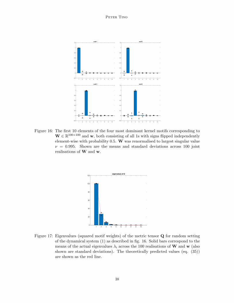
Peter Tino
motif 1
1 2 3 4 5 6 7 8 9 10
-0.2
0
0.2
0.4
0.6
0.8
1
1.2
motif 2
1 2 3 4 5 6 7 8 9 10
-0.2
0
0.2
0.4
0.6
0.8
1
1.2
motif 3
1 2 3 4 5 6 7 8 9 10
-0.2
0
0.2
0.4
0.6
0.8
1
1.2
motif 4
1 2 3 4 5 6 7 8 9 10
-0.2
0
0.2
0.4
0.6
0.8
1
1.2
Figure 16: The first 10 elements of the four most dominant kernel motifs corresponding toW ∈ R100×100 and w, both consisting of all 1s with signs flipped independentlyelement-wise with probability 0.5. W was renormalised to largest singular valueν = 0.995. Shown are the means and standard deviations across 100 jointrealisations of W and w.
eigenvalues of Q
1 2 3 4 5 6 7 8 9 10
0
20
40
60
80
100
120
Figure 17: Eigenvalues (squared motif weights) of the metric tensor Q for random settingof the dynamical system (1) as described in fig. 16. Solid bars correspond to themeans of the actual eigenvalues λi across the 100 realisations of W and w (alsoshown are standard deviations). The theoretically predicted values (eq. (35))are shown as the red line.
38
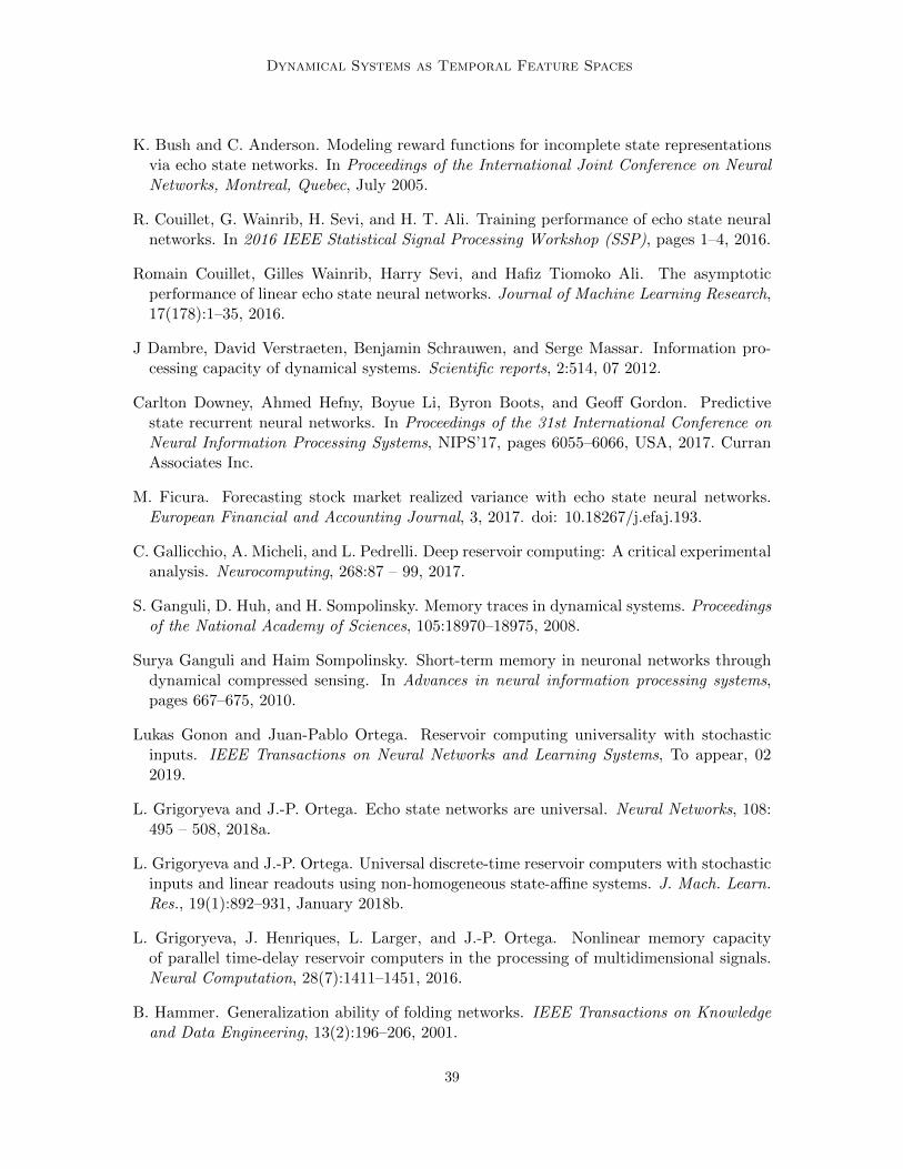
Dynamical Systems as Temporal Feature Spaces
K. Bush and C. Anderson. Modeling reward functions for incomplete state representationsvia echo state networks. In Proceedings of the International Joint Conference on NeuralNetworks, Montreal, Quebec, July 2005.
R. Couillet, G. Wainrib, H. Sevi, and H. T. Ali. Training performance of echo state neuralnetworks. In 2016 IEEE Statistical Signal Processing Workshop (SSP), pages 1–4, 2016.
Romain Couillet, Gilles Wainrib, Harry Sevi, and Hafiz Tiomoko Ali. The asymptoticperformance of linear echo state neural networks. Journal of Machine Learning Research,17(178):1–35, 2016.
J Dambre, David Verstraeten, Benjamin Schrauwen, and Serge Massar. Information pro-cessing capacity of dynamical systems. Scientific reports, 2:514, 07 2012.
Carlton Downey, Ahmed Hefny, Boyue Li, Byron Boots, and Geoff Gordon. Predictivestate recurrent neural networks. In Proceedings of the 31st International Conference onNeural Information Processing Systems, NIPS’17, pages 6055–6066, USA, 2017. CurranAssociates Inc.
M. Ficura. Forecasting stock market realized variance with echo state neural networks.European Financial and Accounting Journal, 3, 2017. doi: 10.18267/j.efaj.193.
C. Gallicchio, A. Micheli, and L. Pedrelli. Deep reservoir computing: A critical experimentalanalysis. Neurocomputing, 268:87 – 99, 2017.
S. Ganguli, D. Huh, and H. Sompolinsky. Memory traces in dynamical systems. Proceedingsof the National Academy of Sciences, 105:18970–18975, 2008.
Surya Ganguli and Haim Sompolinsky. Short-term memory in neuronal networks throughdynamical compressed sensing. In Advances in neural information processing systems,pages 667–675, 2010.
Lukas Gonon and Juan-Pablo Ortega. Reservoir computing universality with stochasticinputs. IEEE Transactions on Neural Networks and Learning Systems, To appear, 022019.
L. Grigoryeva and J.-P. Ortega. Echo state networks are universal. Neural Networks, 108:495 – 508, 2018a.
L. Grigoryeva and J.-P. Ortega. Universal discrete-time reservoir computers with stochasticinputs and linear readouts using non-homogeneous state-affine systems. J. Mach. Learn.Res., 19(1):892–931, January 2018b.
L. Grigoryeva, J. Henriques, L. Larger, and J.-P. Ortega. Nonlinear memory capacityof parallel time-delay reservoir computers in the processing of multidimensional signals.Neural Computation, 28(7):1411–1451, 2016.
B. Hammer. Generalization ability of folding networks. IEEE Transactions on Knowledgeand Data Engineering, 13(2):196–206, 2001.
39
Peter Tino
B. Hammer and P. Tino. Recurrent neural networks with small weights implement definitememory machines. Neural Computation, 15(8):1897–1929, 2003.
J. Hochreiter and J. Schmidhuber. Long short term memory. Neural Computation, 9(8):1735–1780, 1997.
G. Holzmann and H. Hauser. Echo state networks with filter neurons and a delay and sumreadout. Neural Networks, 32(2):244–256, 2009.
H. Jaeger. The ”echo state” approach to analysing and training recurrent neural networks.Technical report gmd report 148, German National Research Center for InformationTechnology, 2001.
H. Jaeger. Short term memory in echo state networks. Technical report gmd report 152,German National Research Center for Information Technology, 2002a.
H. Jaeger. A tutorial on training recurrent neural networks, covering bppt, rtrl, ekf andthe ”echo state network” approach. Technical report gmd report 159, German NationalResearch Center for Information Technology, 2002b.
H. Jaeger and H. Hass. Harnessing nonlinearity: predicting chaotic systems and savingenergy in wireless telecommunication. Science, 304:78–80, 2004.
H. Jaeger, M. Lukosevicius, D. Popovici, and U. Siewert. Optimisation and applicationsof echo state networks with leaky-integrator neurons. Neural Networks, 20(3):335–352,2007.
Li Jing, Caglar Gulcehre, John Peurifoy, Yichen Shen, Max Tegmark, Marin Soljacic, andYoshua Bengio. Gated orthogonal recurrent units: On learning to forget. Neural Com-putation, 31(4):765–783, 2019.
R. E. Kalman. Approach to linear filtering and prediction problems. Journal of BasicEngineering, 82(1):35, 1960.
R. Legenstein and W. Maass. What makes a dynamical system computationally powerful?In S. Haykin, J. C. Principe, T. Sejnowski, and J. McWhirter, editors, New Directions inStatistical Signal Processing: From Systems to Brains, pages 127–154. MIT Press, 2007.
Joseph T. Lizier, Mikhail Prokopenko, and Albert Y. Zomaya. Detecting non-trivial compu-tation in complex dynamics. In Proceedings of the 9th European Conference on Advancesin Artificial Life, ECAL’07, pages 895–904, Berlin, Heidelberg, 2007. Springer-Verlag.
Joseph T. Lizier, Mikhail Prokopenko, and Albert Y. Zomaya. Local measures of informa-tion storage in complex distributed computation. Inf. Sci., 208:39–54, November 2012.
M. Lukosevicius and H. Jaeger. Reservoir computing approaches to recurrent neural networktraining. Computer Science Review, 3(3):127–149, 2009.
W. Maass, T. Natschlager, and H. Markram. Real-time computing without stable states:a new framework for neural computation based on perturbations. Neural Computation,14(11):2531–2560, 2002.
40
Dynamical Systems as Temporal Feature Spaces
G. Manjunath and H. Jaeger. Echo state property linked to an input: Exploring a funda-mental characteristic of recurrent neural networks. Neural Computation, 25(3):671–696,2013. ISSN 0899-7667.
Henryk Minc. Nonnegative Matrices. John Wiley and Sons Ltd-Interscience Series in Dis-crete Mathematics and Optimization, 1988.
O. Obst and J. Boedecker. Guided self-organization of input-driven recurrent neural net-works. In In Guided Self-Organization: Inception. Emergence, Complexity and Compu-tation, pages 319–340. Springer, Berlin, Heidelberg, 2014.
Oliver Obst, Joschka Boedecker, and Minoru Asada. Improving recurrent neural networkperformance using transfer entropy. In Proceedings of the 17th International Confer-ence on Neural Information Processing: Models and Applications - Volume Part II,ICONIP’10, pages 193–200, Berlin, Heidelberg, 2010. Springer-Verlag.
M. C. Ozturk, D. Xu, and J. Principe. Analysis and design of echo state network. NeuralComputation, 19(1):111–138, 2007.
A. Rodan and P. Tino. Minimum complexity echo state network. IEEE Transactions onNeural Networks, 22(1):131–144, 2011.
Ali Rodan and Peter Tino. Minimum complexity echo state network. ieee trans neuralnetw. IEEE transactions on neural networks / a publication of the IEEE Neural NetworksCouncil, 22:131–44, 11 2010. doi: 10.1109/TNN.2010.2089641.
Andre Rohm and Kathy Ludge. Multiplexed networks: reservoir computing with virtualand real nodes. Journal of Physics Communications, 2(8):085007, aug 2018.
M. Rudelson and R. Vershynin. Non-asymptotic theory of random matrices: extreme sin-gular values. In In Proceedings of the International Congress of Mathematicians. VolumeIII, Hindustan Book Agency, New Delhi, pages 1576–1602, 2010.
B. Schrauwen, M. Wardermann, D. Verstraeten, J.J. Steil, and D Stroobandt. Improvingreservoirs using intrinsic plasticity. Neurocomputing, 71(7-9):1159–1171, 2008.
Hava T. Siegelmann and Eduardo D. Sontag. Analog computation via neural networks.Theoretical Computer Science, 131(2):331–360, 1994.
M.D. Skowronski and J.G. Harris. Minimum mean squared error time series classificationusing an echo state network prediction model. In IEEE International Symposium onCircuits and Systems, Island of Kos, Greece, pp. 3153-3156, 2006.
J. Steil. Online reservoir adaptation by intrinsic plasticity for backpropagation-decorrelationand echo state learning. Neural Networks, 20:353–364, 2007.
Tobias Strauss, Welf Wustlich, and Roger Labahn. Design strategies for weight matrices ofecho state networks. Neural Computation, 24(12):3246–3276, 2012. ISSN 0899-7667.
41
Peter Tino
Gouhei Tanaka, Toshiyuki Yamane, Jean Benoit Hroux, Ryosho Nakane, Naoki Kanazawa,Seiji Takeda, Hidetoshi Numata, Daiju Nakano, and Akira Hirose. Recent advances inphysical reservoir computing: A review. Neural Networks, 115:100 – 123, 2019.
P. Tino. Asymptotic fisher memory of randomized linear symmetric echo state networks.Neurocomputing, 298:4–8, 2018.
P. Tino and G. Dorffner. Predicting the future of discrete sequences from fractal represen-tations of the past. Machine Learning, 45(2):187–218, 2001.
P. Tino and B. Hammer. Architectural bias in recurrent neural networks: Fractal analysis.Neural Computation, 15(8):1931–1957, 2004.
P. Tino and A. Rodan. Short term memory in input-driven linear dynamical systems.Neurocomputing, 112:58–63, 2013.
M. H. Tong, A.D. Bicket, E.M. Christiansen, and G.W. Cottrell. Learning grammaticalstructure with echo state network. Neural Networks, 20:424–432, 2007.
Y. Xue, L. Yang, and S. Haykin. Decoupled echo state networks with lateral inhibition.Neural Networks, 20:365–376, 2007.
Izzet B. Yildiz, Herbert Jaeger, and Stefan J. Kiebel. Re-visiting the echo state property.Neural Networks, 35:1 – 9, 2012. ISSN 0893-6080.
Byung-Jun Yoon. Hidden markov models and their applications in biological sequenceanalysis. Current genomics, 10:402–15, 09 2009.
B. Zhang, D. J. Miller, and Y. Wang. Nonlinear system modeling with random matrices:Echo state networks revisited. IEEE Transactions on Neural Networks and LearningSystems, 23(1):175–182, Jan 2012. ISSN 2162-2388. doi: 10.1109/TNNLS.2011.2178562.
42