Dynamical Systems and ChaosPart II: Biology Applications

Lecture 11: Reaction-Di↵usion Systems.

Ilya PotapovMathematics Department, TUT

Room TD325

Reaction-Di↵usion Modeling

Di↵usion is the thermal motion of all (liquid or gas) particlesat temperatures above absolute zero.

I Homogeneous system: probability of finding any randomlyselected molecule inside volume �V is �V/V .

I Homogeneous and thermal equilibrium ! well-stirred(much more nonreactive than reactive collisions happen).

I Sometimes spatial e↵ects play an important role inaddition to temporal e↵ects and we need to includedi↵usive e↵ects to our modeling (spatiotemporal,inhomogeneous, heterogeneous).

I Di↵usion: 1 dimensional (x) – 3 dimensional (x,y,z)

Before going further...

In an assemblage of particles (cells, bacteria, chemicals, animalsetc.) each particle usually moves around in a random way.When this microscopic irregular movement results in somemacroscopic or gross regular motion of the group we can thinkof it as a di↵usion process [J. Murray Mathematical Biology, 3-dedition, Springer, 2003].

Let’s consider simplest 1D case of random walk process.

1D random walk

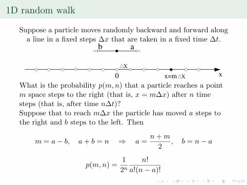
Suppose a particle moves randomly backward and forward alonga line in a fixed steps �x that are taken in a fixed time �t.

X

Xx=m x0

b a

What is the probability p(m,n) that a particle reaches a pointm space steps to the right (that is, x = m�x) after n timesteps (that is, after time n�t)?Suppose that to reach m�x the particle has moved a steps tothe right and b steps to the left. Then

m = a� b, a+ b = n ) a =n+m

2, b = n� a

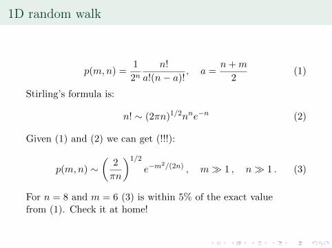
p(m,n) =1

2nn!

a!(n� a)!

1D random walk

p(m,n) =1

2nn!

a!(n� a)!, a =

n+m

2(1)

Stirling’s formula is:

n! ⇠ (2⇡n)1/2nn

e

�n (2)

Given (1) and (2) we can get (!!!):

p(m,n) ⇠✓

2

⇡n

◆1/2

e

�m

2/(2n)

, m � 1 , n � 1 . (3)

For n = 8 and m = 6 (3) is within 5% of the exact valuefrom (1). Check it at home!

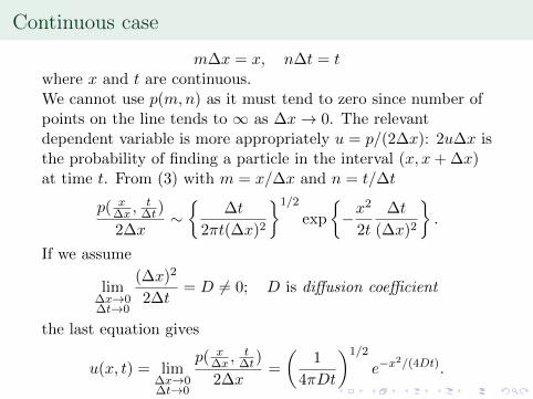
Continuous case

m�x = x, n�t = t

where x and t are continuous.We cannot use p(m,n) as it must tend to zero since number ofpoints on the line tends to 1 as �x ! 0. The relevantdependent variable is more appropriately u = p/(2�x): 2u�x isthe probability of finding a particle in the interval (x, x+�x)at time t. From (3) with m = x/�x and n = t/�t

p( x

�x

,

t

�t

)

2�x

⇠⇢

�t

2⇡t(�x)2

�1/2

exp

⇢�x

2

2t

�t

(�x)2

�.

If we assume

lim�x!0

�t!0

(�x)2

2�t

= D 6= 0; D is di↵usion coe�cient

the last equation gives

u(x, t) = lim�x!0

�t!0

p( x

�x

,

t

�t

)

2�x

=

✓1

4⇡Dt

◆1/2

e

�x

2/(4Dt)

.

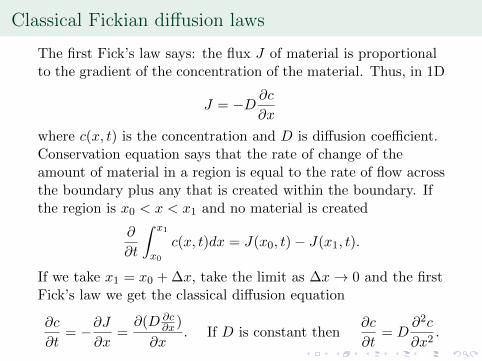
Classical Fickian di↵usion laws

The first Fick’s law says: the flux J of material is proportionalto the gradient of the concentration of the material. Thus, in 1D

J = �D

@c

@x

where c(x, t) is the concentration and D is di↵usion coe�cient.Conservation equation says that the rate of change of theamount of material in a region is equal to the rate of flow acrossthe boundary plus any that is created within the boundary. Ifthe region is x

0

< x < x

1

and no material is created

@

@t

Zx1

x0

c(x, t)dx = J(x0

, t)� J(x1

, t).

If we take x

1

= x

0

+�x, take the limit as �x ! 0 and the firstFick’s law we get the classical di↵usion equation

@c

@t

= �@J

@x

=@(D @c

@x

)

@x

. If D is constant then@c

@t

= D

@

2

c

@x

2

.

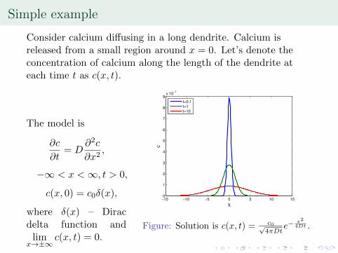
Simple example

Consider calcium di↵using in a long dendrite. Calcium isreleased from a small region around x = 0. Let’s denote theconcentration of calcium along the length of the dendrite ateach time t as c(x, t).

The model is

@c

@t

= D

@

2

c

@x

2

,

�1 < x < 1, t > 0,

c(x, 0) = c

0

�(x),

where �(x) – Diracdelta function andlim

x!±1c(x, t) = 0.

−15 −10 −5 0 5 10 150

1

2

3

4

5

6

7

8

9x 10

−7

x

c

t=0.1

t=1

t=10

Figure: Solution is c(x, t) = c0p4⇡Dt

e

� x

2

4Dt

.

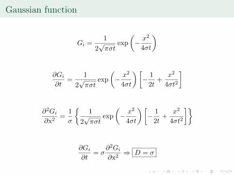
Gaussian function

G

i

=1

2p⇡�t

exp

✓� x

2

4�t

◆

@G

i

@t

=1

2p⇡�t

exp

✓� x

2

4�t

◆� 1

2t+

x

2

4�t2

�

@

2

G

i

@x2=

1

�

⇢1

2p⇡�t

exp

✓� x

2

4�t

◆� 1

2t+

x

2

4�t2

��

@G

i

@t

= �

@

2

G

i

@x2) D = �

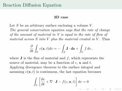
Reaction Di↵usion Equation

3D case

Let S be an arbitrary surface enclosing a volume V .The general conservation equation says that the rate of change

of the amount of material in V is equal to the rate of flow of

material across S into V plus the material created in V . Thus

@

@t

Z

V

c(x, t)dv = �Z

S

J · ds+Z

V

f dv ,

where J is the flux of material and f , which represents thesource of material, may be a function of c, x and t.Applying divergence theorem to the surface integral andassuming c(x, t) is continuous, the last equation becomes

Z

V

@c

@t

+r · J� f(c,x, t)

�dv = 0

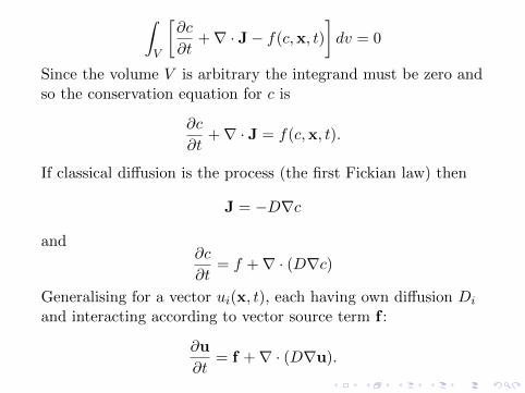
Z

V

@c

@t

+r · J� f(c,x, t)

�dv = 0

Since the volume V is arbitrary the integrand must be zero andso the conservation equation for c is

@c

@t

+r · J = f(c,x, t).

If classical di↵usion is the process (the first Fickian law) then

J = �Drc

and@c

@t

= f +r · (Drc)

Generalising for a vector ui

(x, t), each having own di↵usion D

i

and interacting according to vector source term f :

@u

@t

= f +r · (Dru).

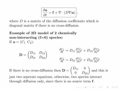
@u

@t

= f +r · (Dru) ,

where D is a matrix of the di↵usiion coe�cients which isdiagonal matrix if there is no cross-di↵usion.

Example of 2D model of 2 chemically

non-interacting (f=0) species:

If u = (C1

C

2

):

D =

✓D

11

D

12

D

21

D

22

◆ @C1@t

= D

11

@

2C1

@x

2 +D

12

@

2C2

@x

2

@C2@t

= D

21

@

2C1

@x

2 +D

22

@

2C2

@x

2

If there is no cross-di↵usion then D =

✓D

11

00 D

22

◆and this is

just two seperate equations, otherwise, two species interactthrough di↵usion only, since there is no source term f .

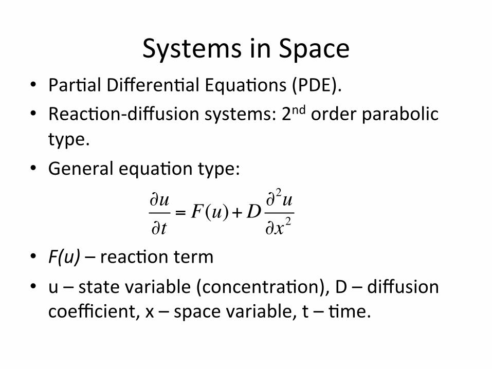
SystemsinSpace•  Par/alDifferen/alEqua/ons(PDE).•  Reac/on-diffusionsystems:2ndorderparabolictype.

•  Generalequa/ontype:

•  F(u)–reac/onterm•  u–statevariable(concentra/on),D–diffusioncoefficient,x–spacevariable,t–/me.

∂u∂t= F(u)+D ∂2u

∂x2

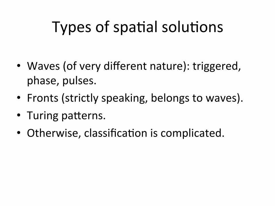
Typesofspa/alsolu/ons

•  Waves(ofverydifferentnature):triggered,phase,pulses.

•  Fronts(strictlyspeaking,belongstowaves).•  TuringpaNerns.•  Otherwise,classifica/oniscomplicated.

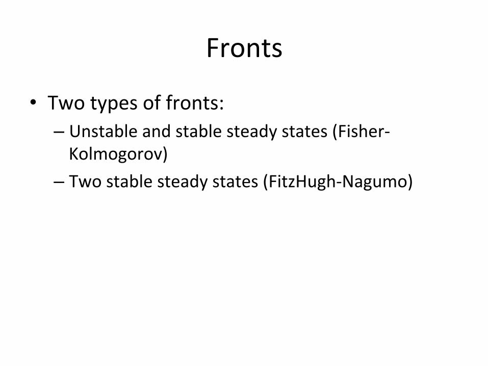
Fronts

•  Twotypesoffronts:– Unstableandstablesteadystates(Fisher-Kolmogorov)

– Twostablesteadystates(FitzHugh-Nagumo)

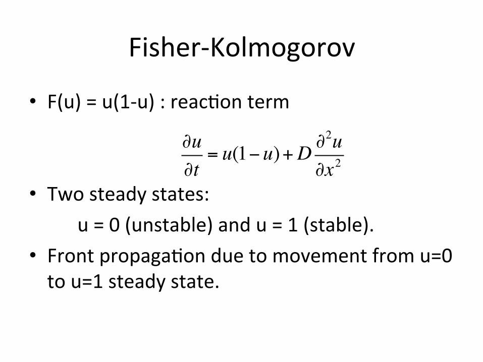
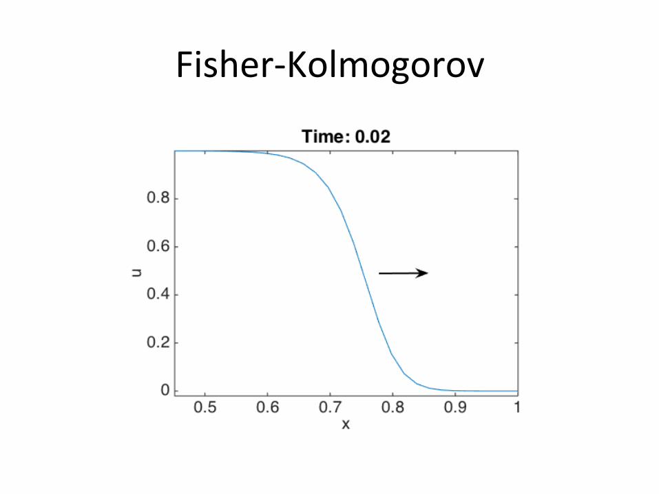
Fisher-Kolmogorov

•  F(u)=u(1-u):reac/onterm

•  Twosteadystates: u=0(unstable)andu=1(stable).

•  Frontpropaga/onduetomovementfromu=0tou=1steadystate.

∂u∂t= u(1−u)+D ∂2u

∂x2

Fisher-Kolmogorov

FitzHugh-Nagumo

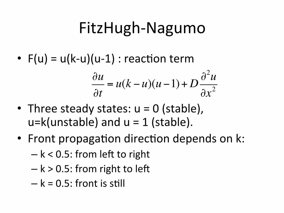
•  F(u)=u(k-u)(u-1):reac/onterm

•  Threesteadystates:u=0(stable),u=k(unstable)andu=1(stable).

•  Frontpropaga/ondirec/ondependsonk:– k<0.5:fromle[toright– k>0.5:fromrighttole[– k=0.5:frontiss/ll

∂u∂t= u(k −u)(u−1)+D ∂2u

∂x2

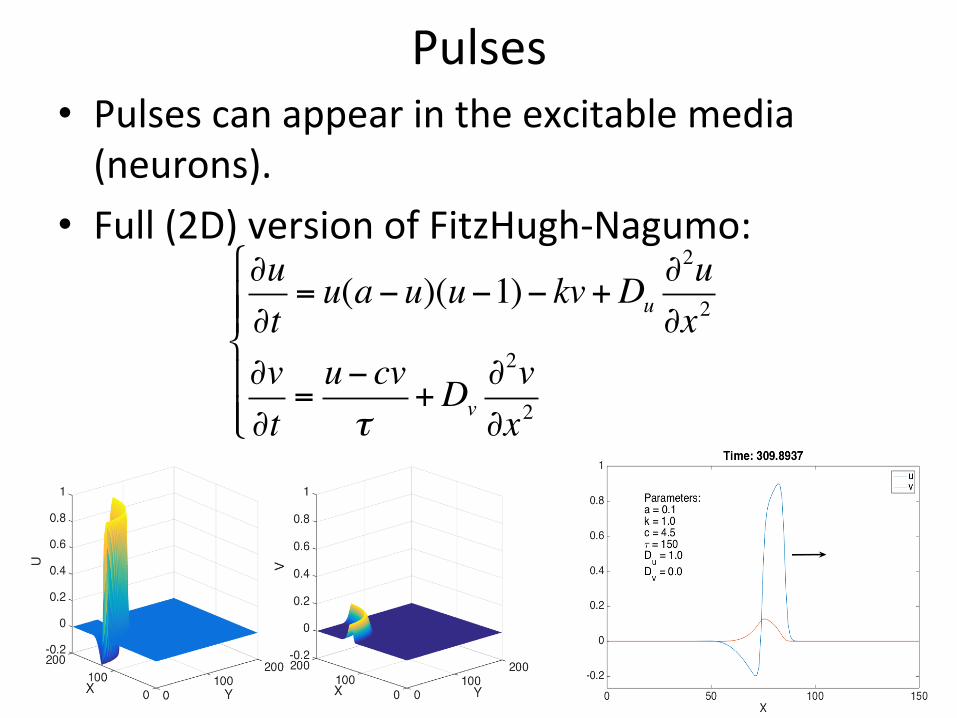
Pulses•  Pulsescanappearintheexcitablemedia(neurons).

•  Full(2D)versionofFitzHugh-Nagumo:∂u∂t= u(a−u)(u−1)− kv+Du

∂2u∂x2

∂v∂t=u− cvτ

+Dv∂2v∂x2

#

$%%

&%%

TuringpaNerns

•  PredictedbyAlanTuring(Enigmacode,firstcomputer,theore/calworkonmorphogenesisin1952).

•  Onlyin1990usingspecializedexperimentaltechniquesinthegroupofDeKepperthefirstTuringpaNernswereshownexperimentally(Phys.Rev.LeN,64,2953,1990).

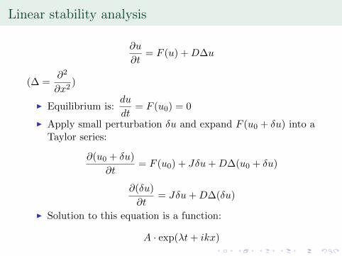
Linear stability analysis

@u

@t

= F (u) +D�u

(� =@

2

@x

2

)

I Equilibrium is:du

dt

= F (u0

) = 0

I Apply small perturbation �u and expand F (u0

+ �u) into aTaylor series:

@(u0

+ �u)

@t

= F (u0

) + J�u+D�(u0

+ �u)

@(�u)

@t

= J�u+D�(�u)

I Solution to this equation is a function:

A · exp(�t+ ikx)

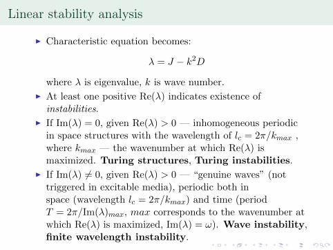
Linear stability analysis

I Characteristic equation becomes:

� = J � k

2

D

where � is eigenvalue, k is wave number.

I At least one positive Re(�) indicates existence ofinstabilities.

I If Im(�) = 0, given Re(�) > 0 — inhomogeneous periodicin space structures with the wavelength of l

c

= 2⇡/kmax

,where k

max

— the wavenumber at which Re(�) ismaximized. Turing structures, Turing instabilities.

I If Im(�) 6= 0, given Re(�) > 0 — “genuine waves” (nottriggered in excitable media), periodic both inspace (wavelength l

c

= 2⇡/kmax

) and time (periodT = 2⇡/Im(�)

max

, max corresponds to the wavenumber atwhich Re(�) is maximized, Im(�) = !). Wave instability,finite wavelength instability.

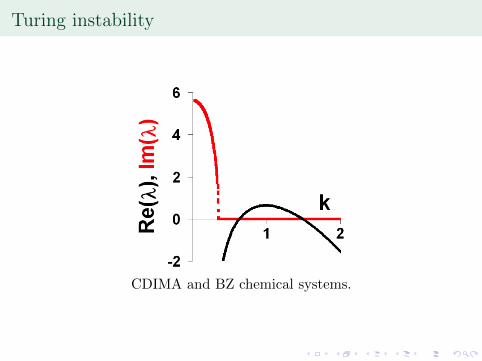
Turing instability

CDIMA and BZ chemical systems.

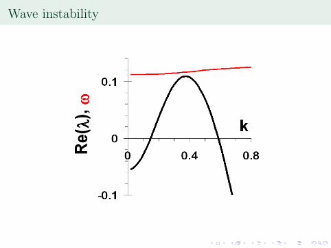
Wave instability

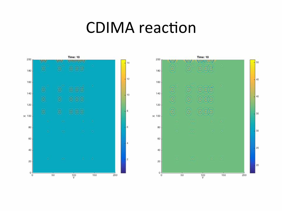
CDIMAreac/on

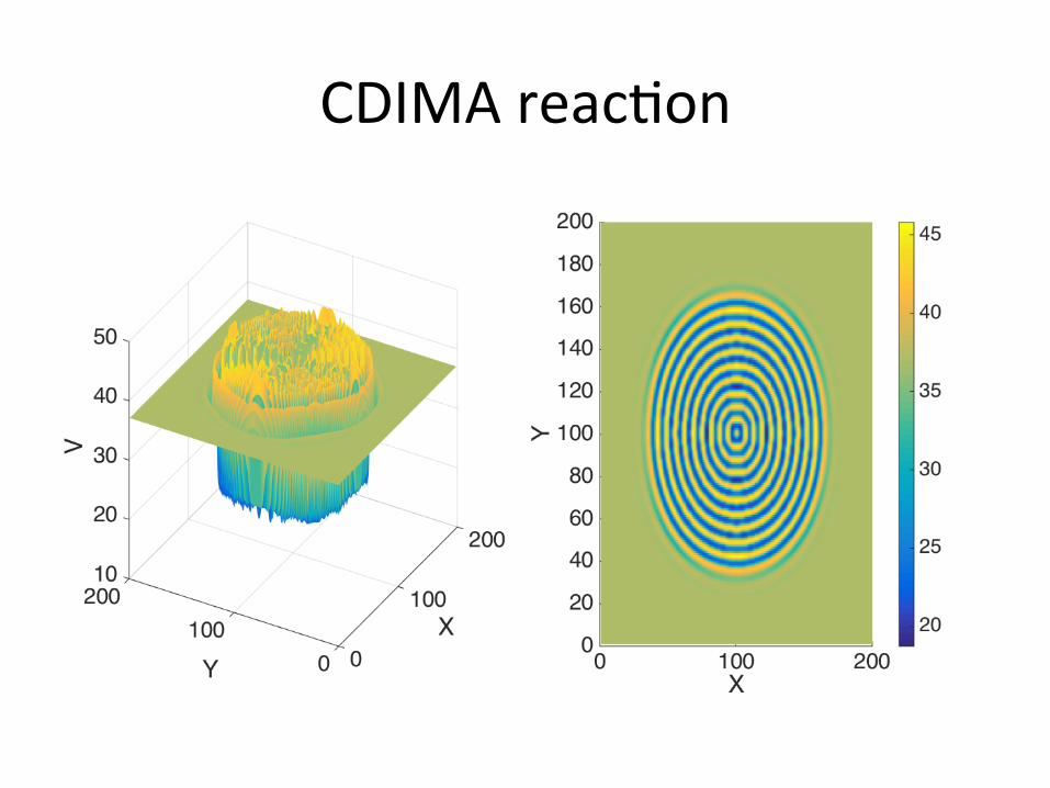
CDIMAreac/on

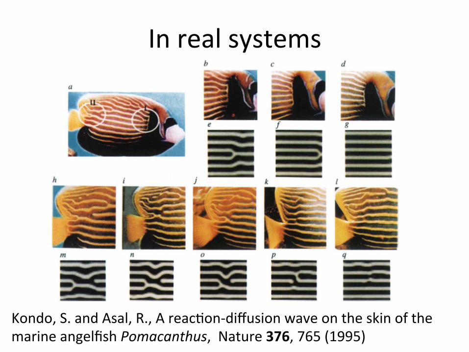
Inrealsystems

Kondo,S.andAsal,R.,Areac/on-diffusionwaveontheskinofthemarineangelfishPomacanthus,Nature376,765(1995)

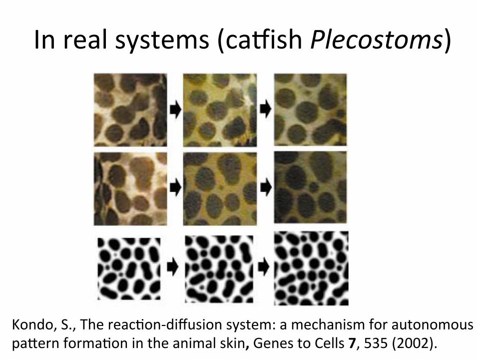
Inrealsystems(cagishPlecostoms)

Kondo,S.,Thereac/on-diffusionsystem:amechanismforautonomouspaNernforma/onintheanimalskin,GenestoCells7,535(2002).

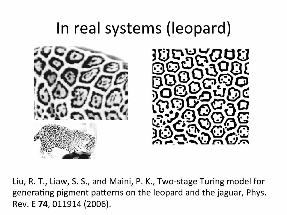
Inrealsystems(leopard)

Liu,R.T.,Liaw,S.S.,andMaini,P.K.,Two-stageTuringmodelforgenera/ngpigmentpaNernsontheleopardandthejaguar,Phys.Rev.E74,011914(2006).

References

•  J.D.Murray,Mathema/calBiology.I.AnIntroduc/on,3rded,ISBN0-387-95223-3,Springer,2002.

•  A.M.Turing,TheChemicalBasisofMorphogenesis,Phil.Trans.RoyalSoc.,237,641,pp.37—72.

Appendix:spa/alpaNernsWavesinoscillatorymedia

Spirals in hydrodynamics. E. Bodenschatz, W. Pesch, G. Ahlers. Annu. Rev. Fluid Mech. v. 32 (2000), 709

Spirals in Xenopus Laevis oocytes. Scale bar = 100 µm. J. D. Lechleiter, L. M. John, P. Camacho. Biophys. Chem. 72 (1998) 123.

Spirals in cones and pineapples. P. Atela, C. Golé, and S. Hotton, J. Nonlinear Sci. v.12 (2002) 641

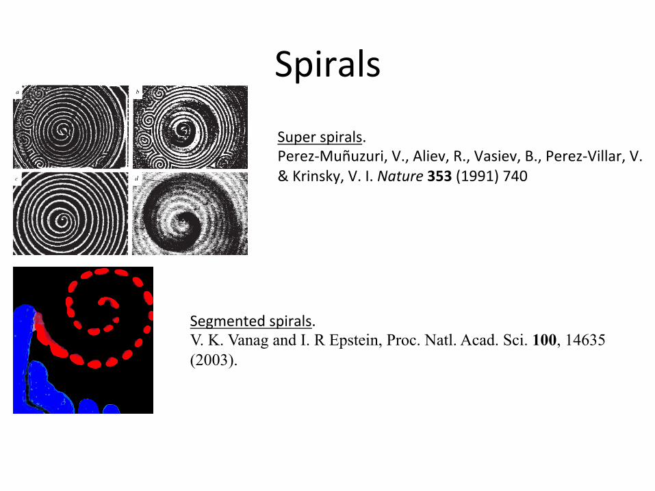
Spirals

Superspirals.Perez-Muñuzuri,V.,Aliev,R.,Vasiev,B.,Perez-Villar,V.&Krinsky,V.I.Nature353(1991)740

Segmentedspirals.V. K. Vanag and I. R Epstein, Proc. Natl. Acad. Sci. 100, 14635 (2003).

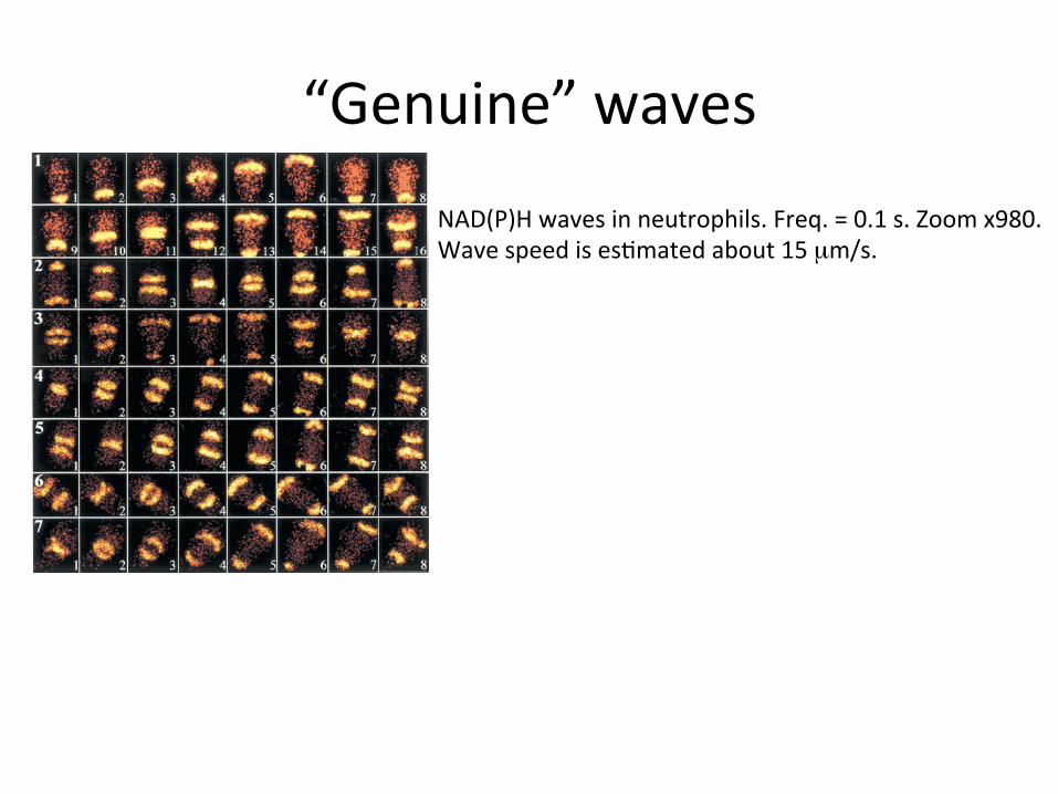
“Genuine”waves

NAD(P)Hwavesinneutrophils.Freq.=0.1s.Zoomx980.Wavespeedises/matedabout15µm/s.