dynamical study of metallic clusters using the statistical method of

Computer Physics Communications 182 (2011) 1013–1026

Contents lists available at ScienceDirect

Computer Physics Communications

www.elsevier.com/locate/cpc

Dynamical study of metallic clusters using the statistical method of time seriesclustering

S.K. Lai a,b,∗, Yu-Ting Lin a, P.J. Hsu a,b, S.A. Cheong c

a Complex Liquids Laboratory, Department of Physics, National Central University, Chungli 320, Taiwanb Molecular Science and Technology Program, Taiwan International Graduate Program, Academia Sinica, Taipei 115, Taiwanc Division of Physics and Applied Physics, School of Physics and Mathematical Sciences, Nanyang Technological University, SPMS-04-01, 21 Nanyang Link, Singapore 637371, Singapore

a r t i c l e i n f o a b s t r a c t

Article history:Received 14 September 2009Received in revised form 24 October 2010Accepted 29 December 2010Available online 5 January 2011

Keywords:Molecular dynamics simulationTime series data analysisMetallic clusters

We perform common neighbor analysis on the long-time series data generated by isothermal Brownian-type molecular dynamics simulations to study the thermal and dynamical properties of metallic clusters.In our common neighbor analysis, we introduce the common neighbor label (CNL) which is a group ofatoms of a smaller size (than the cluster) designated by four numeric digits. The CNL thus describestopologically smaller size atomic configurations and is associated an abundance value which is thenumber of “degenerate” four digits all of which characterize the same CNL. When the cluster is in itslowest energy state, it has a fixed number of CNLs and hence abundances. At nonzero temperatures,the cluster undergoes different kinds of atomic activities such as vibrations, migrational relocation,permutational and topological isomer transitions, etc. depending on its lowest energy structure. As aresult, the abundances of CNLs at zero temperature will change and new CNLs with their respective newabundances are created. To understand the temperature dependence of the CNL dynamics, and henceshed light on the cluster dynamics itself, we employ a novel method of statistical time series analysis. Inthis method, we perform statistical clustering at two time scales. First, we examine, at given temperature,the signs of abundance changes at a short-time scale, and assign CNLs to two short-time clusters. Quasi-periodic features can be seen in the time evolution of these short-time clusters, based on which wechoose a long-time scale to compute the long-time correlations between CNL pairs. We then exploitthe separation of correlation levels seen in these long-time correlations to extract strongly-correlatedcollections of CNLs, which we will identify as effective variables for the long-time cluster dynamics. It isfound that certain effective variables show subtleties in their temperature dependences and these thermaltraits bear a delicate relation to prepeaks and main peaks seen in clusters Ag14, Cu14 and Cu13Au1. Wetherefore infer from the temperature changes of effective variables and locate the temperatures at whichthese prepeaks and principal peaks appear, and they are evaluated by comparing with those deducedfrom the specific heat data.

© 2011 Elsevier B.V. All rights reserved.

1. Introduction

At very low temperatures, atoms in a metallic cluster executesolid-like vibration. The description of this oscillatory motion inthe presence of an external probe such as temperature is quitedifferent from that in the bulk. Whereas in a bulk system thethermal response of atoms are treated individually the same ow-ing to the translational symmetry, atoms in a cluster under thesame condition are, however, realized by their whereabouts lo-cations since their geometrical sites have much bearing on howthey respond and hence the cluster properties. Consider, for ex-ample, a 14-atom pure cluster and a 38-atom bimetallic cluster

* Corresponding author at: Complex Liquids Laboratory, Department of Physics,National Central University, Chungli 320, Taiwan.

E-mail address: [email protected] (S.K. Lai).

0010-4655/$ – see front matter © 2011 Elsevier B.V. All rights reserved.doi:10.1016/j.cpc.2010.12.047

Ag32Cu6 at their respective lowest energy states. The former [1,2]can be differentiated generally into three broad kinds of atoms,namely, floating (adatom), surface and central atoms and the lat-ter [3], on the other hand, can be categorized coarse grainedly intosurface and central atoms. Such a classification of atoms by thepositions they reside is instructive at higher temperatures and pro-vides a practical means in quantitative analysis of the microscopicdynamics of clusters. In two recent communications [2,4], we haveapplied this strategy of partitioning atoms in a cluster to investi-gate the velocity autocorrelation function; we deduced from thisdynamic quantity and its Fourier-transformed function, the powerspectrum, the average temperature at which a cluster melts. Wedemonstrated that these dynamic variables can be employed toinfer the melting temperature Tm of a cluster and the predictedvalue is reasonably close to that estimated from the principal peakposition of the specific heat CV (widely accepted to be the melt-

http://dx.doi.org/10.1016/j.cpc.2010.12.047

http://www.ScienceDirect.com/

http://www.elsevier.com/locate/cpc

mailto:[email protected]

http://dx.doi.org/10.1016/j.cpc.2010.12.047

1014 S.K. Lai et al. / Computer Physics Communications 182 (2011) 1013–1026

ing temperature Tm). In the course of interpreting the dynamicresults, an attempt was made to explain the anomalous increaseof the relative root–mean–square bond length fluctuation constant

[2,4] δ = 1n(n−1)

∑ni=1

∑nj �=i

√〈r2

i j(t)〉t−〈ri j(t)〉2t

〈ri j(t)〉twhose aberrant thermal

response occurs not at Tm but at a much lower temperature. Inthese latter works [2,4], attention was drawn to tracking down si-multaneously the instantaneous relative bond length ri j(t) in δ fori j-atoms. A careful and thorough analysis of ri j(t) at each temper-ature reveal indeed the complex dynamics of individual atoms. Itis now understood, for instance, that the anomalous increase of δ

at lower temperatures for Cu14 or Ag14 [2,4] is due mainly to themigrational relocations of the floating atom. As the temperature ofthe cluster climbs up further, the ri j(t) indicates an increase in thefrequency of permutational isomer transitions among the floatingand surface atoms, and such exchange activities continue until thecentral atom participates finding its way out via permutating witha surface or floating atom. The cluster should by then approach Tm .Although the analysis using ri j is dynamically fruitful, it is nev-ertheless a complicated procedure since a synchronous follow-upof different ri js (atomic pairs of floating-surface, surface-surface,central-surface, etc.) must be effected for a conclusive descriptionto be reached. Moreover, the ri j variable does not give much in-sight into the factors that govern the atomic dynamics at differenttemperatures.

In this work, we turn to a more practical means of studyingthe dynamical behavior of clusters. Rather than examining ri j si-multaneously for different pairs of i j-atoms, we scrutinize insteada group of atoms which comprises a root pair and its commonneighbors. This kind of the common neighbor analysis (CNA) findsits application in a wide range of problems in bulk systems. We il-lustrate in this paper that the CNA can equally well be applied tostudy the dynamical motion of atoms in a cluster. Differing fromthe usual simulation method where the time development of theposition coordinates and velocities of atoms in a cluster are usedto explore the cluster dynamics from calculating such quantities asthe root–mean–square displacement, velocity autocorrelation func-tion, etc., we introduce here a new scheme — based on CNA andtime series clustering — to understand the time evolution.

In a typical molecular dynamics (MD) simulation running overtens of millions of time steps, the sheer volume of data con-tained in the large number of displacement time series makesanalyzing and understanding the underlying physics a challeng-ing task. Simple visualization of these simulation data in the formof a movie brings forth too much subjective bias. An objectiveway to reduce data complexity is to effect time series cluster-ing, a class of methods that has found applications in diverseareas of business, science and technology. In time series cluster-ing, the objective is to group together time series data sets withsimilar dynamical features so that a much smaller collection ofdynamically distinct clusters is obtained. Broadly, the time seriesclustering methods can be classified into model-based methods[5–11] and correlations-based methods [12–18]. Both these meth-ods have been reviewed by Liao [19] and we refer the interestedreaders to this article for more details. Since the physics behindnanocluster melting is not yet fully understood, we cannot ap-ply existing model-based methods to our problem, as this wouldintroduce modeling biases. Neither can we simply adapt existingcorrelations-based methods, as our goal is to develop a mechanis-tic picture of the melting process. Instead, we choose to developa new correlations-based time series clustering method that is ahybridization of the methods developed by Rummel et al. [14,18]and Tumminello et al. [13,15]. In our method, we draw attentionto novel ways of analyzing the correlation matrix and demonstrate,by illustration of several small clusters using CNA, how the ef-fective variables (to be defined below) are obtained and applied

to describe the dynamics of our physical system. We should em-phasize that the time series clustering method was developed forlarger complex systems in mind, and has in fact been success-fully applied to finance [20,21], neuroscience [22–26], and mete-orology [27–29]. We have, for instance, very recently applied themethod to financial markets (500–3000 degrees of freedom) [30]and global positioning system networks (100 degrees of freedom)[31]. In these two systems, the dynamical time scales are not wellseparated. Employing the method of partial hierarchical cluster-ing [30], we, however, managed to extract the effective variablesas well as their dynamics. In contrast, the dynamical time scalesare well separated in the metallic clusters chosen here, up to veryhigh temperatures. This important qualitative difference betweenthe financial/geophysical systems and metallic clusters confers anadded advantage to the time series clustering method, because theseparation of dynamical time scales translates into a separation ofcorrelation levels in each of the long-time windows. There is thusno cause for alarm in the event that the dynamical time scales arenot well separated. Armed with this time series clustering scheme,we proceed to interpret the microscopic time series data whichwe will obtain from an isothermal Brownian-type MD simulationon several metallic clusters.

The present paper is organized as follows. In Section 2, we givea brief summary of the CNA following the definition of Honeycuttand Andersen [32] and introduce the method of time series clus-tering on multiple time scales in detail. We devote a significantportion of the method to explain its advantage. In the discussionsbelow, we refer extensively to various statistical observations madefrom the time series of the common neighbor labels which aresole elements in the CNA. Our intention is to explain clearly toreaders how quasi-regular synchronies in the short-time dynam-ics can be converted into reliable long-time correlations, basedon which we then identify the effective variables. We shall notdescribe the isothermal Brownian-type MD simulations that wereused to generate the microscopic time series data. We refer theinterested readers, however, to our previous works for technicaldetails [1,2,4]. Throughout this section, for concreteness, we useCu13 as an illustrative example to inaugurate the statistical timeseries clustering methodology. In Section 3, we give a quantita-tive discussion of the results derived from the time series analysisfirst for Ag14, and then for Cu14 and Cu13Au1; we make a compar-ison between Cu14 and Cu13Au1, delving into the possible inter-pretations of the dynamics. With regard to the melting scenario,we infer Tm from the temperature-dependences of the time se-ries data and compare its value with corresponding one deducedfrom CV . Since the CV for Ag14, Cu14 and Cu13Au1 have been re-ported previously [1,2], we will therefore simply cite the results orjust summarize them without further description. Finally, we givea conclusion in Section 4.

2. Methodology: Common neighbor analysis and time seriesanalysis

2.1. Common neighbor analysis

In our CNA, we examine the neighborhoods around all pairsof atoms in the cluster, and note these at each time step in theform of four-digit common neighbor labels (CNL), {c1, c2, c3, c4}.In this analysis, we say that there is a bonded root-pair atomsif the distance between them is rb � 1.2r0, r0 being the nearestneighbor separation. Therefore, for a given root-pair atoms, weset c1 = 1 if they are bonded, or c1 = 2 if they are not. Next,we set c2 equal to the number of atoms bonded simultaneouslyto both root-pair atoms. We call these the common neighborsof the root-pair atoms. Then, we set c3 equal to the number ofbonds among the common-neighbor atoms. Finally, we can have

S.K. Lai et al. / Computer Physics Communications 182 (2011) 1013–1026 1015

topologically-distinct neighborhoods with CNL that have exactlythe same first three digits. These are distinguished by the fourthdigit c4 = 1,2, . . . in their CNLs. As examples, we illustrate howtwo such CNLs are determined for the Cu13 cluster in Fig. 1.

2.2. Time series analysis

In this section, we describe the general framework for extract-ing effective variables using the statistical method of time seriesclustering at multiple time scales. Effective variables are collectionsof microscopic variables which evolve in time synchronously. Theseare identified in two stages. First, we examine the time series dataover a sequence of non-overlapping short-time windows. Withineach short-time window, microscopic variables are assigned to var-ious short-time clusters based on a chosen short-time statistic. Forconcreteness, let us consider the CNLs {1321} and {2101} of Cu13shown in Fig. 1, in an isothermal Brownian-type MD simulationrunning over 1×107�t (each time step �t = 0.001 ps). We choosea short-time window of δsw = 10�t . At T = 0 K, the CNLs {1321}and {2101} have, respectively, a total of thirty and six “degener-ate” {c1, c2, c3, c4} and these are called their abundances. For T > 0,these abundances change from time to time, as a result of atomicmotions within the cluster. We identify the abundance pi,k of theith CNL at the kth short-time window as the microscopic variable,and define the short-time statistic by the CNL correlation level

Si,k =⎧⎨⎩

+1, �pi,k > 0;0, �pi,k = 0;−1, �pi,k < 0,

(1)

where �pi,k = pi,k+1 − pi,k . Based on the values of this short-time statistic Si,k , we can then assign microscopic variables tothree different short-time clusters at each short-time step k. Ofthese, only the Si,k = +1 and Si,k = −1 short-time clusters providedynamical information on the behavior of the cluster. A simpleway to visualize the dynamics of the short-time statistic Si,k overlong times is to make a density plot, whereby the (i,k) cell isfilled if Si,k = +1 (or Si,k = −1 if we are interested in the otherdynamically-informative short-time cluster). In Fig. 2(a)–(b), weshow such density plots for the short-time clusters Si,k = ±1 ofCu13 at T = 800 K. In these figures, we label the CNLs by indices.A look-up table is constructed to track down the CNL by referringto the CNL index (see Table 1). Returning to Fig. 2(a)–(b), it is ingeneral not easy to discern regularities in the density plots whenwe show the entire duration of the simulation. These regularitiesbecome clearer when we restrict ourselves to a shorter time du-ration (but still long compared to δsw), as shown in Fig. 3(a)–(b)for T = 800 K. We see quasi-periodic features in the density plotsthat involve more CNLs and vary at a shorter period (compare,for example, to that at T = 400 K (not shown)). Also, we havestudied the density plots obtained using different short-time win-dows, δsw = 10 and 50�t . We find that a quasi-periodic featurewith a period between 1000 to 3000δsw can be seen more clearlyfor δsw = 10�t . This tells us that the dynamical information cap-tured by our short-time statistic Si,k is robust with respect to ourchoice of this short-time window δsw . This robustness is impor-tant, because we can then select a long-time window δLW based onthe unambiguous observed period and carry out a coarse-grainedanalysis in the second stage of our effective variable extractionframework. To effect the long-time dynamics, we construct withineach long-time window a long-time correlation matrix C , whosematrix elements are defined by

Cij = (1 − δi j)

m∑ 1

2

∣∣Si,k S j,k(Si,k + S j,k)∣∣ (2)

k=1

Fig. 1. The CNLs {1321} (top) and {2101} (bottom) for the Cu13 cluster. In this fig-ure, atoms are shown as solid spheres, while bonds between atoms are shown asconnecting rods. The root-pair atoms are colored black, and labeled A and B, whiletheir common-neighbor atoms are colored green. In the top subfigure, we find thatA and B are bonded root-pair atoms, and share three common neighbors. This isthe first topologically-distinct neighborhood where two bonds are found among thethree common-neighbor atoms. Hence the CNL is {1321}. In the bottom subfigure,we find that A and B are not bonded root-pair atoms, but they share a commonneighbor. Since there is only one common-neighbor atom, there is no bond withinthe common neighborhood of A and B. Hence we denote the CNL by {2101}. (Forinterpretation of the references to colors in this figure, the reader is referred to theweb version of this article.)


Fig. 2. CNL correlation levels (a) Si,k = +1 and (b) Si,k = −1 of Cu13 calculated atT = 800 K for short-time clusters.

where m is the number of short-time window steps within thelong-time window. Note that the long-time correlation matrix C issymmetric, i.e. Cij = C ji , and the value of the matrix element Cij

is the number of times the CNL correlation levels Si,k and S j,k areassigned to the same short-time cluster within the chosen long-time window. The diagonal elements Cii are set to zero, becausethey provide no cross-correlational information on the cluster dy-namics. The long-time correlation matrix C , thus contains matrixelements of different correlation levels. These are the product ofdynamics operating on different time scales (such as the collec-tion of time scales shown in Fig. 4). Dynamics at time scales muchshorter than the long-time window will self-average, producing alow background correlation level contribution to C . Dynamics attime scales longer than the long-time window, on the other hand,will produce correlation levels rising above the background. Evenwithout knowing the precise nature of the dynamical structures,we expect dynamics with time scales closest to the long-time scaleto produce stronger correlation levels, and dynamics with timescales further from the long-time scale to produce weaker corre-lation levels. If these dynamical time scales are widely separated,there will be a corresponding clean separation of correlation lev-els in the long-time correlation matrix C . Where this separation ofcorrelation levels is found, we can directly decompose C into dis-tinct submatrices, whereby the large matrix elements Cij of C arefound only within these submatrices, and any other submatrices

Table 1Look-up table for CNL and its corresponding index for Cu13 at 800 K.

CNL index CNL CNL index CNL

1 1 1 0 1 48 2 3 3 12 2 1 0 1 49 1 4 3 13 1 2 0 1 50 2 4 3 14 2 2 0 1 51 1 5 3 15 1 3 0 1 63 1 4 4 16 2 3 0 1 64 2 4 4 17 1 4 0 1 65 1 5 4 1

17 1 2 1 1 66 2 5 4 118 2 2 1 1 78 2 4 5 119 1 3 1 1 79 1 5 5 120 2 3 1 1 80 2 5 5 121 1 4 1 1 81 1 6 5 133 1 3 2 1 93 1 5 6 134 2 3 2 1 94 2 5 6 135 1 4 2 1 95 1 6 6 136 2 4 2 1 109 1 6 7 137 1 5 2 1 149 1 5 2 247 1 3 3 1

Fig. 3. Same as Fig. 2 but for selected shorter time durations.

of C are distinguished by their matrix elements Cij significantlysmall. Based on this decomposition of C , we identify the col-lections of strongly-correlated CNLs associated with such distinctsubmatrices as our effective variables.

As a concrete illustration of this long-time clustering procedureto identify effective variables, we perform a Brownian-type MD runfor Cu13 at T = 700 K. For a total number of 1 × 107�t simulation


time steps, we choose the long-time window to be δLW = 2000δsw .Advancing the long-time window at intervals of 1000δsw , we ob-tain 999 overlapping long-time windows each of which is associ-ated with a C matrix. In Fig. 5(a), we give the long-time correla-tion matrix of the first long-time window, which runs from δsw to2000δsw . As we can see, there are several distinct groups of matrix

Fig. 4. Schematic diagram showing different time scales.

elements: Cij > 200, Cij ∼ 80, Cij ∼ 60, Cij ∼ 15, and Cij < 10, rep-resenting distinct correlation levels within the long-time window.The frequency of occurrence of Cij assuming the same numericalvalue in the matrix C (see Fig. 5(a)) plotted against the magnitudeof this numerical value of Cij is depicted in Fig. 6. In particular, wefind the Cij � 200 correlation level very strong, and are very wellseparated from the rest of the correlation levels. From the corre-lation matrix C , one can extract the effective variables in terms ofcollections of CNLs (microscopic variables) which are grouped to-gether on the basis of a cutoff value of Cij (see Fig. 6).

Let us digress to describe how the effective variables are deter-mined. Fig. 7 is the flow chart showing the numerical procedurethat we follow to extract the effective variable. We start by firstscrutinizing the histogram for the frequency of occurrence of thecorrelation level elements Cij calculated for Cu13 at T = 700 K.As indicated in Fig. 6, there is a large gap separating some highcorrelation level elements (whose Cij � 200) from other lowerones (Cij � 82). We then read of from Fig. 6 a cutoff value of

(a)

Fig. 5. (a) Matrix elements of correlation level matrix C calculated for Cu13 at T = 700 K. (b) Re-ordered matrix elements of the matrix C given in (a). The submatricesshaded grey yield the same effective variables.


(b)

Fig. 5. Continued.

Cij which we denote as Ccut . Choosing Ccut = 141, we next turnto Fig. 5(a) again and read in column by column the elementsCij of the correlation matrix C . For the first column of Cij , i = 1,we check the inequality Cij > Ccut for row elements j = 1,2, . . . ,of C1 j . If the answer is positive, we group these CNLs, otherwisewe move on to the second column. For example, the first twocolumns in Fig. 5(a) produce no CNL that matches the inequal-ity criterion. However, a group of five CNLs satisfies C3 j > Ccut forthe 3rd column and they are {1211,2211,2321,1431,1541}. A fur-ther check for Cij > Ccut among the (contracted group of) CNLs{2211,2321,1431,1541} in this third column group is effected im-mediately. The result of this verification is that four CNLs remain.Next, we proceed to do similar checking among the three CNLs{2321,1431,1541} for Cij > Ccut . This procedure is continued hier-archically, and we confirm that the 3rd column yields an effectivevariable {1211,2211,2321,1431,1541}. We should emphasize thatthis kind of hierarchical checking among CNLs has to be carriedout in a manner until group(s) of CNLs are sorted out. The latteris/are then labeled as effective variable(s). For this first-window C ,

the above hierarchical procedure is repeated for columns 4th, 7th,8th, 10th, 11th, 13th and 14th (i.e. for i > 3). A comparison ofthe effective variables obtained in all columns is finally effectedto ensure that there is no overlapping effective variables. Follow-ing this numerical scheme, two effective variables emerge, namely,{1221,1431,1541,2211,2321} and {1321,1551,2331}. We shouldmention at this point that we can re-order the long-time corre-lation matrix displayed in Fig. 5(a) to that in Fig. 5(b). In this re-ordered C , notice that the off-diagonal matrix elements within twosubmatrices are all greater than 200, and the matrix elements inthese two submatrices are much larger than the matrix elementsof any other submatrices whose Cij are all significantly smallerthan 200 (for example, {1101,2101,1421}). One can thus identifyin this re-ordered long-time correlation matrix two diagonal blocksand they are in fact associated with the same effective variables.In general, when we slide our long-time window along the sim-ulation period, the number of the effective variables can change,and so can CNL and number of CNLs within each effective variable.To examine the long-time variations of the effective variables, and


determine their dynamical time scales, as well as the nature andcharacter of their long-time dynamics, we need to automate theextraction process. The key to this automation (shown in Fig. 7)is the separation of correlation levels, as shown in Fig. 6. Un-like existing methods [23–25,28], the present method is designedspecifically for identifying effective variables from very large timeseries data sets in an automated and unbiased fashion, even whenthe natures and structures of the effective variables change slowlywith time. By sliding the long-time window along the time axis,the method will also be able to identify dynamical time scales atwhich these effective variables evolve, provided that these effectivetime scales are significantly longer than the short-time scale.

Fig. 6. Frequency of occurrence of the element Cij assuming the same numericalvalue in the correlation matrix C of Fig. 5(a) for the first long-time window vs. themagnitude of this numerical value Cij for Cu13 calculated at 700 K.

3. Results and discussions

We are now in a position to apply the time series analysisto study the dynamical properties of metallic clusters. We firstpresent results for Ag14, and then for Cu14 and Cu13Au1, in amanner that allows comparison between pure and bimetallic clus-ters.

3.1. Pure cluster Ag14

We have previously studied [2] the dynamical properties ofAg14. The energy histogram and its lowest and lower energy struc-tures are given in Ref. [2] to which the readers are referred fordetails. At temperatures T � 140 K, this cluster is in its lowestenergy state — an icosahedron with a floating atom or adatom re-siding near a three-atoms base. The first excited state (in additionto the ground state) occurs at T = 150 K and it persists until nearT = 200 K at which temperature the second excited state emerges.Note that, apart from the distorted geometry of the icosahedron,the first and second excited states differ from the lowest energystate in that a deformed four-atoms base is located near the float-ing atom. At T = 300 K, only the lowest, first and second excitedstates are found (see Fig. 2 in Ref. [2]). More excited states appearfor T > 300 K.

An instructive description of the long-time dynamics of thecluster Ag14 can be obtained by showing at each temperature howfrequently the effective variable appears in all of the 999 long-timewindows. Since the effective variable is associated with collectionsof CNLs, it is convenient in the following discussion to label thelatter by an effective variable index (EVI). Table 2 is a look-uptable for tracking down the effective variable. At given tempera-ture, the occurrence of effective variables in all of the long-timewindows are recorded and plotted against EVI. Let us begin byscrutinizing the density plots of the short-time clusters Si,k = ±1obtained at T = 100 K using δsw = 10�t . They are depicted inFig. 8(a)–(b). Based on the quasi-period seen in the density plots,

Fig. 7. Flow chart showing the numerical procedure for extracting the effective variables.


Table 2Look-up table for the effective variables labeled by numeric integer index for Ag14.

Effectivevariable index

Number ofCNL

CNLs

1 8 1101 1201 1311 1541 2201 2211 2321 24312 5 1211 1321 1431 1551 23313 4 1201 1311 2321 24314 2 2201 22115 3 1321 1551 23316 2 1211 14317 3 1541 2211 23218 5 1211 1431 1541 2211 23219 2 2211 2321

10 2 1201 221111 3 1201 2211 232112 3 1101 2211 232113 2 1201 131114 6 1211 1431 1541 2101 2211 232115 4 1101 2201 2321 243116 3 1201 1311 221117 3 1211 2211 232118 2 1101 220119 3 1201 1311 243120 2 2101 221121 2 1551 233122 4 1321 1551 2101 233123 2 1211 232124 2 1321 233125 3 1101 2201 243126 2 1541 221127 2 2201 231128 2 1211 221129 2 2321 233130 2 1541 232131 3 1211 1431 221132 2 1211 210133 4 1211 2101 2211 232134 4 1211 1541 2211 232135 2 1101 131136 3 1211 2101 221137 2 1431 233138 2 1311 221139 2 1101 210140 3 1101 1201 210141 2 1101 120142 2 1201 232143 2 1211 233144 5 1101 1201 1311 2211 232145 3 1101 2201 231146 3 1101 2101 220147 3 1211 1311 221148 4 1211 1321 1431 233149 3 1211 1421 221150 3 1211 1321 233151 3 1321 1431 233152 4 1101 1201 1311 221153 4 1101 1201 1311 232154 3 1201 1311 2321

we choose δLW = 2000δsw , and slide the long-time window in1000δsw increments to generate 999 long-time windows, for a to-tal simulation time steps of 1 × 107�t . At this temperature, wesee in Fig. 9(a) only two effective variables, EVI-1 (hereafter we la-bel the ith effective variable index by an integer i as EVI-i) andEVI-2. Checking the look-up Table 2, they are {1101,1201,1311,

1541,2201,2211,2321,2431} and {1211,1321,1431,1551,2331},respectively. Since the energy histogram (see Fig. 2 in Ref. [2]) in-dicates that only the ground state is present at T = 100 K, thesetwo effective variables describe solely vibrational motion. Compar-ing the CNLs in the two effective variables with those in the lowestenergy structure (Fig. 10), we see more CNLs of EVI-1 than theground state structure and the EVI-1 accounts for the harmonictype oscillatory motion and captures atomic configurations withlarger distortion in contrast to that displayed by EVI-2.

In Fig. 9(a)–(b), we show how the occurrence frequencies of ef-fective variables depend on temperature, from T = 100 to 1500 K,in intervals of 100 K. We see that as we increase the temperature(T > 100 K), the number of effective variables increases rapidly toaround 30 for T = 200–300 K after which it decreases rapidly toaround 5 by T = 700 K. More interestingly, we find that EVI-1 andEVI-2 appear more frequently as we go from T = 100 to 200 K, butbecome less frequent at higher temperatures. As the occurrencefrequencies of EVI-1 and EVI-2 decline, we notice a correspondingrise in the occurrence frequency of EVI-5, which, from Table 2, con-sists of the CNLs {1321,1551,2331}. The EVI-5 peaks at T = 400 K,and thereafter decreases with increasing temperature, but it con-tinues to be detected until at T = 900 K where it disappears iden-tically. While these dynamic behaviors unfold, EVI-24 whose CNLsare {1321,2331} emerges at a temperature as low as T = 200 K,and it keeps growing with increasing temperature. Since the CNL


Fig. 8. CNL correlation levels (a) Si,k = +1 and (b) Si,k = −1 of Ag14 calculated at T = 100 K for short-time clusters.

(a) (b)

Fig. 9. Occurrence of effective variables in the total number of long-time windows for Ag14 for temperature range (a) T = 100–1000 K and (b) T = 1100–1500 K. In thesefigures, the integers in {. . .} are the effective variable index found at temperature T . Consult the look-up Table 2 for strongly-correlated CNLs corresponding to the effectivevariable index.


Fig. 10. Seven CNLs for the ground state configurations of Ag14.

{1551} has one of its root-pair atoms which is the central atomof the icosahedron, it is reasonable to consider the CNL {1551} asmaintaining a solid-like structure, and naturally interpret the dis-appearance of EVI-5 as indicating the cluster’s tendency to melt.Based on this interpretation, the melting temperature possibly fallsin the range 800 � Tm � 900 K. This melting temperature is lessthan Tm = 920 K which we previously [2] deduced from the mainmaximum position of specific heat, but agrees with that we in-ferred from the analysis of the power spectral density (see Fig. 6in Ref. [2]).

As pointed out above, EVI-24 appears more frequently with in-creasing temperature from T � 200 K and is seen to replace EVI-5for T � 900 K. It would therefore be interesting to examine thecorrelation level matrix element {1321,2331} in each of the long-time windows. To this end, we read of the value of this elementin the correlation level matrices of all 999 long-time windows anddenote their average value by Cav . Fig. 11 displays Cav plotted as afunction of T . We find that there is a maximum at T ≈ 960 K.

3.2. Pure and bimetallic clusters: Cu14 and Cu13Au1

We turn next to a comparative study of the time series analysisclustering for Cu14 and Cu13Au1. For Cu14, the readers are again re-

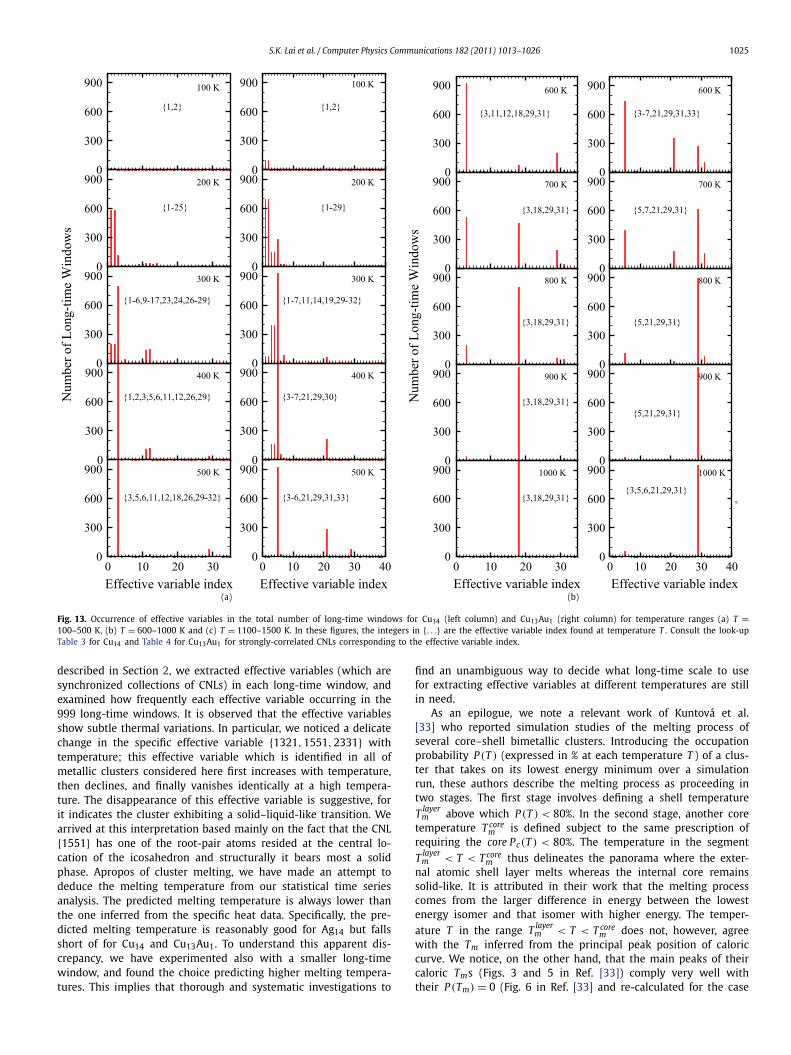
ferred to Ref. [4] for its energy histogram (Fig. 3 in Ref. [4]) and thelowest energy and lower excited states (Fig. 2 in Ref. [4]), whereasfor Cu13Au1 its energy histogram is shown in Fig. 12 and its low-est energy and lower excited states are found in Ref. [1] (Fig. 5 inthis reference). We note, first of all, that the lowest energy stateof Cu14 persists up to T = 110 K which is 40 K lower than thatin Cu13Au1. The first excited state of Cu14 emerges at T = 120 K,and there is no sign of the second excited state up till T = 500 K.In contrast, the first excited state of the bimetallic cluster Cu13Au1occurs at 150 < T � 160 K, after which the second and third ex-cited states appear and these two excited states are seen to growall the way up to T = 500 K. These differences in atomic config-urations, which can be probed as functions of temperature, arereflected in subtle changes of effective variables. For Cu14, onenotices from Fig. 13(a) that EVI-1 which is {1101,1201,1311,

1541,2201,2211,2321,2431} and EVI-2 which is {1211,1321,

1431,1551,2331} (see Table 3 to look up effective variables forCu14) first climb up as the temperature increases from T = 100to 200 K after which they decline to about three times less inmagnitude at T = 300 K and vanish identically at T = 500 K. Thesame trends are seen for Cu13Au1 (Fig. 13(a)) except that EVI-1 which is {1101,1201,1311,1541,2201,2211,2321,2431} andEVI-2 which is {1211,1321,1431,1551,2331} (see Table 4 to look


Fig. 11. Averaged value Cav (over all long-time windows) of correlation level ele-ments {1321,2331} that are read from Cij vs. T (in Kelvin) for Ag14.

up effective variables for Cu13Au1) ascend more rapidly but alsodescend fast (for instance, at T = 300 K they are already 7 timesless in magnitude than those at T = 200 K) and these effectivevariables disappear at T = 400 K which contrasts to T = 500 Kin Cu14. Another set of effective variables whose occurrence fre-quencies rise and fall with increasing temperature is EVI-11 andEVI-12 for Cu14, and EVI-3 and EVI-4 for Cu13Au1. These effec-tive variables peak between T = 300 and 400 K for Cu14, and atT = 300 K for Cu13Au1. At T = 600 K, they become vanishinglysmall both for Cu14 and Cu13Au1. Since the first and second ex-cited states of Cu14 and with addition also the third for Cu13Au1emerge at these temperature ranges, the thermal variations of thissecond set of effective variables must be intimately related to theobserved prepeaks of specific heats (at approximately 400 K forCu14 and 300 K for Cu13Au1). The temperature change of theseeffective variables agrees with the position of the prepeak max-imum which is at higher temperature for Cu14 and lower forCu13Au1.

Apart from the up and down characteristics of these two sets ofeffective variables, we see from Fig. 13(a)–(c) a conspicuous tem-perature response of the effective variable {1321,1551,2331} (EVI-3 for Cu14, and EVI-5 for Cu13Au1, see Tables 3 and 4). These CNLshave the largest abundance values among the seven ground-stateCNLs of both Cu14 and Cu13Au1. Just as in Ag14, the occurrencefrequency of this effective variable rises rapidly to its peak valuebetween T = 400 to 500 K in Cu14 and at T = 400 K in Cu13Au1,and thereafter declines to identically zero at T = 1100 and 1300 K,respectively. Following the argument used for Ag14, the meltingtemperature is predicted to fall in the range 1000 � Tm � 1100 Kfor Cu14 and 1200 � Tm � 1300 K for Cu13Au1. For Cu14, this melt-ing temperature underestimates that inferred from the main peakposition of CV (Tm ≈ 1257 K, see Fig. 2 in Ref. [1]) by about 150 K.For Cu13Au1, the melting temperature predicted using the time se-ries clustering method is closer to that deduced from the mainpeak position of C V (Tm ≈ 1357 K, see Fig. 3 in Ref. [1]).

In closing this section, we would like to comment on the Tm

obtained from the main maximum position of C V and that calcu-lated in the time series clustering method. In the former, Tm is anaverage temperature estimated by the drastic change of cluster’saverage potential energy over a finite temperature range, whereasin the latter it appeals to the abundances of CNLs whose valueschange temporally and rapidly with temperature. In the time se-ries clustering method, the strongly-correlated CNLs are groupedtogether to become effective variables on the basis of the valuesof correlation level elements. For the presently considered clusters,

Fig. 12. Energy histogram for Cu13Au1.

the vanishment of an effective variable and its corresponding CNLswhich we scrutinize over a specific range of temperature permitsus to infer Tm , albeit approximately due to larger temperature in-tervals (100 K) used in simulations.

4. Conclusions

We have generated long-time series data sets for metallic clus-ters Cu13, Ag14, Cu14, and Cu13Au1 using an isothermal Brownian-type MD simulation. From the time evolution of atomic config-urations recorded at different temperatures, the CNLs and theirassociated abundances were calculated. We performed statisticalclustering on the change of CNL-abundance time series at a short-time scale, and then another statistical clustering based on theshort-time correlation between CNL-abundance changes at a long-time scale. We found robust dynamical features in the short-timeclustering using a short-time scale of δsw = 10�t (�t = 0.001 ps).However, we are at present unable to unambiguously select along-time scale for the long-time clustering. Accordingly, we havechosen — by visual inspection of the short-time clustering densityplots — to work with a long-time scale of 2000δsw . To test the rea-sonableness of this choice, we effected sliding window analysis onthe simulation duration, advancing the long-time window at inter-vals 1000δsw to generate 999 overlapping long-time windows. Thissliding window procedure was repeated for different temperatures.Using the long-time correlation matrix decomposition algorithm


Table 3Look-up table for the effective variables labeled by numeric integer index for Cu14.


Number ofCNL

CNLs

1 8 1101 1201 1311 1541 2201 2211 2321 24312 5 1211 1321 1431 1551 23313 3 1321 1551 23314 2 1211 23215 2 2211 23216 5 1211 1431 1541 2211 23217 6 1201 1311 1431 1541 2211 24418 6 1321 1441 1551 1661 2331 24519 2 1201 2211

10 2 1541 221111 2 1211 143112 3 1541 2211 232113 4 1101 2201 2321 243114 3 1201 1311 221115 2 1211 233116 4 1201 1311 2321 243117 2 2201 221118 2 1321 233119 4 1201 1311 1541 221120 4 1321 1551 2101 233121 3 1211 2101 232122 6 1211 1431 1541 2101 2211 232123 2 1201 131124 2 2321 243125 2 1211 210126 4 1211 1541 2211 232127 2 1551 233128 3 1101 2201 243129 3 1211 2211 232130 4 1211 2101 2211 232131 2 1211 221132 3 1211 1431 221133 2 1101 210134 2 1311 221135 2 1431 2331

Table 4Look-up table for the effective variables labeled by numeric integer index for Cu13Au1.


Number ofCNL

CNLs

1 8 1101 1201 1311 1541 2201 2211 2321 24312 5 1211 1321 1431 1551 23313 2 1211 14314 3 1541 2211 23215 3 1321 1551 23316 5 1211 1431 1541 2211 23217 2 2211 23218 6 1211 1431 1541 2101 2211 23219 2 2101 2211

10 2 1551 233111 3 1201 1311 221112 6 1201 1211 1421 2101 2211 232113 4 1311 1321 1551 233114 2 1201 221115 4 1201 1311 2321 243116 2 2201 221117 2 1211 232118 4 1321 1551 2101 233119 4 1101 2201 2321 243120 3 1101 2211 232121 3 1211 2211 232122 7 1101 1211 2101 2201 2211 2321 243123 5 1211 1421 2101 2211 232124 4 1201 1311 2211 244125 2 1201 131126 2 2321 243127 4 1211 1541 2211 232128 2 1541 221129 2 1321 233130 4 1211 2101 2211 232131 2 1211 221132 2 1541 232133 3 1211 2101 221134 2 1101 210135 2 1311 221136 3 1101 1201 210137 2 1101 220138 2 1201 232139 2 1431 2331


(a) (b)

Fig. 13. Occurrence of effective variables in the total number of long-time windows for Cu14 (left column) and Cu13Au1 (right column) for temperature ranges (a) T =100–500 K, (b) T = 600–1000 K and (c) T = 1100–1500 K. In these figures, the integers in {. . .} are the effective variable index found at temperature T . Consult the look-upTable 3 for Cu14 and Table 4 for Cu13Au1 for strongly-correlated CNLs corresponding to the effective variable index.

described in Section 2, we extracted effective variables (which aresynchronized collections of CNLs) in each long-time window, andexamined how frequently each effective variable occurring in the999 long-time windows. It is observed that the effective variablesshow subtle thermal variations. In particular, we noticed a delicatechange in the specific effective variable {1321,1551,2331} withtemperature; this effective variable which is identified in all ofmetallic clusters considered here first increases with temperature,then declines, and finally vanishes identically at a high tempera-ture. The disappearance of this effective variable is suggestive, forit indicates the cluster exhibiting a solid–liquid-like transition. Wearrived at this interpretation based mainly on the fact that the CNL{1551} has one of the root-pair atoms resided at the central lo-cation of the icosahedron and structurally it bears most a solidphase. Apropos of cluster melting, we have made an attempt todeduce the melting temperature from our statistical time seriesanalysis. The predicted melting temperature is always lower thanthe one inferred from the specific heat data. Specifically, the pre-dicted melting temperature is reasonably good for Ag14 but fallsshort of for Cu14 and Cu13Au1. To understand this apparent dis-crepancy, we have experimented also with a smaller long-timewindow, and found the choice predicting higher melting tempera-tures. This implies that thorough and systematic investigations to

find an unambiguous way to decide what long-time scale to usefor extracting effective variables at different temperatures are stillin need.

As an epilogue, we note a relevant work of Kuntová et al.[33] who reported simulation studies of the melting process ofseveral core–shell bimetallic clusters. Introducing the occupationprobability P (T ) (expressed in % at each temperature T ) of a clus-ter that takes on its lowest energy minimum over a simulationrun, these authors describe the melting process as proceeding intwo stages. The first stage involves defining a shell temperatureT layer

m above which P (T ) < 80%. In the second stage, another coretemperature T core

m is defined subject to the same prescription ofrequiring the core Pc(T ) < 80%. The temperature in the segmentT layer

m < T < T corem thus delineates the panorama where the exter-

nal atomic shell layer melts whereas the internal core remainssolid-like. It is attributed in their work that the melting processcomes from the larger difference in energy between the lowestenergy isomer and that isomer with higher energy. The temper-ature T in the range T layer

m < T < T corem does not, however, agree

with the Tm inferred from the principal peak position of caloriccurve. We notice, on the other hand, that the main peaks of theircaloric Tms (Figs. 3 and 5 in Ref. [33]) comply very well withtheir P (Tm) = 0 (Fig. 6 in Ref. [33] and re-calculated for the case


(c)

Fig. 13. Continued.

Ag32Co13 (Fig. 14(a)) using the Brownian-type MD). These resultsare rationalized by the relatively larger size and core–shell struc-tures of clusters. For small clusters such as Ag14 and Cu14, we findthe criterion P (Tm) � 20% (yielding ≈920 K for Ag14 (Fig. 14(b))and ≈1270 K for Cu14 (Fig. 14(c))) is more compatible with theTm deduced at the main maximum position of C V . Structurallythis is reasonable since in these two clusters the atomic distribu-tions are almost all surface atoms and the difference between thelowest energy isomer and the next higher one is about five timessmaller (for instance, roughly 0.1 eV for Ag14) than the bimetalliccluster Cu13Au1. The time series clustering method reported herecan only be used to predict an approximate Tm because of thelarger temperature interval (100 K) used in the simulations. It isour intention to pinpoint Tm and this is now feasible due to ourrecent development [34] of a parallelized code of the isothermalBrownian-type MD that permits doing simulation at a controllabletemperature interval (10 K).

Acknowledgement

This work is supported by the National Science Council, Taiwan(NSC96-2112-M-008-018-MY3).

Fig. 14. Normalized occupation probability P (T ) of finding the cluster in the lowestenergy minimum for (a) Ag32Co13, (b) Ag14 and (c) Cu14.

References

[1] Tsung-Wen Yen, S.K. Lai, N. Jakse, J.L. Bretonnet, Phys. Rev. B 75 (2007) 165420;S.K. Lai, W.D. Lin, K.L. Wu, W.H. Li, K.C. Lee, J. Chem. Phys. 121 (2004) 1487.

[2] Tsung-Wen Yen, P.J. Hsu, S.K. Lai, e-J. Surf. Sci. Nanotech. 7 (2009) 149.[3] A. Rapallo, G. Rossi, R. Ferrando, A. Fortunelli, Benjamin C. Curley, Lesley D.

Lloyd, G.M. Tarbuck, R.L. Johnston, J. Chem. Phys. 122 (2005) 194308.[4] P.J. Hsu, J.S. Lo, S.K. Lai, J.F. Wax, J.L. Bretonnet, J. Chem. Phys. 129 (2008)

194302. This reference summarizes some recent studies of clusters which aredevoted to using velocity autocorrelation function.

[5] V.V. Gafiychuk, B.Yo. Datsko, J. Izmaylova, Physica A 341 (2004) 547.[6] A.M. Alonso, J.R. Berrendero, A. Hernández, A. Justel, Comput. Statist. Data

Anal. 51 (2006) 762.[7] M.A. Juárez, M.F.J. Steel, CRiSM Paper No. 06-14, Warwick University, 2006.[8] C. Allefeld, S. Bialonski, Phys. Rev. E 76 (2007) 066207.[9] L. Bauwens, J.V.K. Rombouts, Econ. Rev. 26 (2007) 365.

[10] M. Corduas, D. Piccolo, Comput. Statist. Data Anal. 52 (2008) 1860.[11] S. Frühwirth-Schnatter, S. Kaufmann, J. Business Econ. Statist. 26 (2008) 78.[12] S.M. Focardi, F.J. Fabozzi, Quant. Fin. 4 (2004) 417.[13] M. Tumminello, T. Aste, T. Di Matteo, R.N. Mantegna, Proc. Natl. Acad. Sci.

USA 102 (2005) 10421.[14] C. Rummel, G. Baier, M. Müller, Europhys. Lett. 80 (2007) 68004.[15] M. Tumminello, F. Lillo, R.N. Mantegna, Europhys. Lett. 78 (2007) 30006.[16] T. Heimo, G. Tibély, J. Saramäki, K. Kaski, J. Kertész, Physica A 387 (2008) 5930.[17] G. Innocenti, D. Materassi, J. Phys. A: Math. Theor. 41 (2008) 205101.[18] C. Rummel, Phys. Rev. E 77 (2008) 016708.[19] T.W. Liao, Pattern Recognition 38 (2005) 1857.[20] R.N. Mantegna, Euro. Phys. J. B 11 (1999) 193.[21] V. Plerou, P. Gopikrishnan, B. Rosenow, L.A.N. Amaral, H.E. Stanley, Phys. Rev.

Lett. 83 (1999) 1471.[22] S. Bialonski, K. Lehnertz, Phys. Rev. E 74 (2006) 051909.[23] U. Lee, S. Kim, K.-Y. Jung, Phys. Rev. E 73 (2006) 041920.[24] G. Baier, M. Müller, U. Stephani, H. Muhle, Phys. Lett. A 363 (2007) 290.[25] G.J. Ortega, R.G. Sola, J. Pastor, Neurosci. Lett. 447 (2008) 129.[26] A.K. Roopun, R.D. Traub, T. Baldeweg, M.O. Cunningham, R.G. Whittaker,

A. Trevelyan, R. Duncan, A.J.C. Russell, M.A. Whittington, Epilepsy & Behav-ior 14 (2009) 39.

[27] J. Basak, A. Sudarshan, D. Trivedi, M.S. Santhanam, J. Machine Learning Res. 5(2004) 239.

[28] M. Cogliati, P. Britos, R. García-Martínez, in: Artificial Intelligence in Theory andPractice, Springer, Boston, 2006, pp. 305–314.

[29] S. Bivona, G. Bonanno, R. Burlon, D. Gurrera, C. Leone, Physica A 387 (2008)5910.

[30] Y.W. Goo, T.W. Lian, W.G. Ong, W.T. Choi, S.A. Cheong, Financial atoms andmolecules, http://arxiv.org/pdf/0903.2099.

[31] W. Wang, S.A. Cheong, A GPS time series clustering analysis of the 16 October2007 Milford Sound Earthquake, presented at the 2010 Western Pacific Geo-physics Meeting, 22–25 June, 2010, Taipei, Taiwan.

[32] J.D. Honeycutt, H.C. Andersen, J. Phys. Chem. 91 (1987) 4950.[33] Z. Kuntová, G. Rossi, R. Ferrando, Phys. Rev. B 77 (2008) 205431.[34] P.J. Hsu, S.K. Lai, unpublished (2011).

http://arxiv.org/pdf/0903.2099

dynamical study of metallic clusters using the statistical method of

Documents