dynamical modelling of a metabolic reaction network

Dynamical Modelling of a MetabolicReaction Network

JOAN GONZALEZ HOSTA

Masters’ Degree ProjectStockholm, Sweden Sep 2009

XR-EE-RT 2009:019

Dynamical modelling of a metabolic reaction network

Master Thesis in Automatic Control, KTH

Joan Gonzalez Hosta

Supervisor: Elling W. Jacobsen

External contact: Veronique Chotteau

Stockholm-Barcelona, 2009

1

I would like to specially thank my supervisor Elling W. Jacobsen for making me realise when I was wrong and making me have a better understanding of everything, the responsible person in the KTH Division of Bioprocess Veronique Chotteau for always being able to find time for my doubts in her busy timetables and for the motivation she gave me in hard times and the “guy of the experiments” Andreas Andersson for his extra-hours in order to try to have the data on time and for his kindness. I’m amazed of all the things that I have learnt.

Joan Gonzalez Barcelona, 2009-08-11

2

Abstract In a cell culture system, a lot of compounds are involved considering the ones contained in the medium (extracellular) and the intracellular environment. Studies of the different system behaviours adopted due to variations in the medium concentrations are typically based on empirical or statistical approaches when working with such an amount of compounds. In this paper is presented a method to develop a dynamical model of a cell culture system which can predict the evolution of the medium compounds and cell growth along the time for this kind of systems. The method has been implemented as a standardised tool that can be used for any kind of biological system when a pre-defined metabolic network and data of different states are available. In parallel to this project, a medium where the exact concentrations of all the compounds are known and should let the cells live properly have been developed by the KTH Division of Bioprocess. The system corresponding to the experiments carried out to develop the medium has been modelled using the proposed method. The results have been analysed and the conclusions, requirements and drawbacks of the model have been discussed.

3

Table of contents 1. Introduction ......................................................................................................................... 5 1.1. Basic concepts ................................................................................................................................. 5 1.1. The aim of the master thesis ............................................................................................................ 5 1.2. The aim of the master thesis ............................................................................................................ 6

2. Initial description ................................................................................................................. 7 2.1. System equations description .......................................................................................................... 7 2.1.1. The quasi steady-state assumption ............................................................................................... 8 2.2. The system object of the study ........................................................................................................ 9 2.3. The available network .................................................................................................................... 10 2.4. The experimental data ................................................................................................................... 11 2.4.1. Estimation of the values of the consumption/production rates and concentrations in a determined

system state..................................................................................................................................... 13 2.4.2. The available experimental data ................................................................................................. 14

3. The Modelling Method ...................................................................................................... 17 3.1. Design of the Macroscopic Stoichiometric Model ........................................................................... 17 3.1.1. System description for the macroscopic design ........................................................................... 18 3.1.2. The Kernel Matrix and the Elementary Flux Modes...................................................................... 20 3.1.3. The Metatool procedure ............................................................................................................. 23 3.1.3.1. Reactions that don’t involve internal metabolites ..................................................................... 26 3.1.4. Calculation of the macroscopic reactions stoichiometry .............................................................. 26 3.2. Design of the reduced dynamical model......................................................................................... 27 3.2.1. Reaction kinetics modelling......................................................................................................... 28 3.2.2. Fitting the maximal kinetic rates coefficients ......................................................................... 30

4. Implementation ................................................................................................................. 33 4.1. Method tools ................................................................................................................................. 33 4.2. Result tools.................................................................................................................................... 37

5. Results and analysis ........................................................................................................... 42 5.1. Results for the available network ................................................................................................... 42 5.1.1. Results analysis ........................................................................................................................... 44 5.2. The new network ........................................................................................................................... 46 5.3. Data usage..................................................................................................................................... 48 5.3.1. The problem with Serine and Asparagine .................................................................................... 48 5.3.2. Samples selection ....................................................................................................................... 48 5.4. Results for the new network .......................................................................................................... 49 5.5. The new objective function ............................................................................................................ 54 5.6. Final results ................................................................................................................................... 55 5.7. Time simulation ............................................................................................................................. 61 5.7.1. Simulation implementation ......................................................................................................... 61 5.7.2. Simulation Results ...................................................................................................................... 62

4

6. Conclusions, drawbacks and improvements ...................................................................... 68 6.1. Conclusions of the method ............................................................................................................ 68 6.2. Conclusions of the results for the system object of study ............................................................... 71 6.3. Future works ................................................................................................................................. 72

7. References ......................................................................................................................... 73

Appendix I: The available network ........................................................................................ 74 Appendix II: The new network............................................................................................... 78 Appendix III: Calculations from data (ci and qi) ..................................................................... 81 Appendix IV: Elementary Flux Modes and all their corresponding macroscopic reactions

Amac.................................................................................................................................. 83 Appendix V: Time simulations of CT3D1, CT6D1, CT9D1, CT10D1 and CT12D1 ...................... 88 Appendix VI: Function codes ................................................................................................. 96

5

1. Introduction The phenomenon that maintains the cells living by providing feeding and consequently also energy is the metabolism. The metabolism is the set of chemical reactions that allows these organisms to grow and reproduce, maintain their structure and adapt to the environments where they have to live. The biochemical reactions that form this metabolism consist, basically, in the transformation of chemical compounds (or metabolites) into other ones. In order to study the cells behavior or how they evolve in different conditions, the reactions that form the metabolism have been tried to model into equations. The fact is that due to the huge number of reactions and compounds that form the metabolism, this modeling has been focused in some sets of reactions that are part of the metabolism and form a system themselves. Depending on the field of study, the target compounds or the processes of interest, the selection of the reactions and the metabolites that will be involved in the model can change for the same system. The collection of these reactions is what we call a metabolic reaction network.

1.1. Basic concepts A metabolic reaction network is a complex system formed by several metabolites which are linked by biochemical reactions. The change in the concentrations of these metabolites depends basically on the magnitudes of the fluxes of the reactions where they are involved and, at the same time, the magnitude of the fluxes depend on the concentrations of the metabolites that are involved in every reaction. A metabolic pathway is a consecution of reactions within the network that starting from one metabolite leads to another one. So, according to the theory, the metabolic pathways within the metabolic network that will be

Figure 1. 1 Scheme of a metabolic network; metabolites (nodes) and reactions (arrows) [1]

6

followed by the different compounds will change depending on the concentrations of the metabolites involved in these pathways. The magnitude of the fluxes of the different pathways will determine the metabolites production or consumption rates and the change in their concentrations.

For every reaction, the metabolites that are consumed are called substrates (their concentration decreases when the reaction takes place) and the ones that are produced are known as products (in this case, the concentration increases).

A simple example of a typical metabolic network of mammal cells is represented in figure 1.1. The nodes represent the metabolites that are considered in the network and the arrows represent the reactions that link these metabolites. The direction of the arrows means the sign of the reaction flux. For example, the reaction v1 transforms the metabolite G into G6P; through this reaction, the concentration of the metabolite G (the substrate) will decrease while the concentration of G6P (the product) will increase and the velocity is the flux value of v1.

In order to carry out studies in this field, cells are cultivated, usually in reactors or flasks. A cell culture is the system formed by a medium where the cells live and is the environment that they have to interact with, and the cells themselves. The medium will also contain metabolites that will be used in the biochemical reactions that form the metabolism.

Then, considering a cell culture, two different kinds of metabolites can be found; the internal metabolites, which are the ones inside the cell, and the external metabolites, that are the compounds that the medium contains. The metabolic network describes the reactions that relate the metabolites (internal and external) that are wanted to be considered in the system.

In the example in figure 1.1 the metabolites in a grey circle represent the external metabolites, which are also linked to internal metabolites through reactions. These processes are what allow the interaction of the cells with the medium.

1.2. The aim of the master thesis The aim of the master thesis is to develop a method that produces a mathematical model that allow us to predict the behaviour of a determined cell culture system given the reactions of a pre-defined metabolic network and implement it. This means a dynamical model that can predict how the concentrations of the metabolites of interest in the medium and the cell growth will evolve.

It has to be considered that only the external metabolites concentrations can be measured, known or controlled, so the inputs in the resulting model have to be variables only referring to concentrations of external metabolites.

So concretely what the model should be able to do is, given an initial values of the considered external metabolites concentrations, to predict the consumption/production rates of these metabolites, and then be able to simulate the dynamic behaviour of the metabolites along the time using this predicted values.

7

2. Initial description Next a description of the information that is available before starting to apply any methodology or doing any calculations is explained. This available information consists basically in the equations that reach the metabolic stoichiometry, the parameters and conditions of the system that is wanted to model, a stoichiometric model of the metabolic network and the available data and the implicit information in it.

2.1. System equations description The main elements of the metabolic network model, as said previously, are (1) the metabolites involved and their concentrations and (2) the reactions that produced the variation of these concentrations. The stoichiometric coefficients denote the proportion of substrate and product molecules involved in every reaction. For example, considering the reaction: → 2

The stoichiometric coefficients would be -1 for glucose and 2 for the lactate, which means that with one mole of glucose 2 of lactate can be produced. We could also say that to get one mole of lactate 0.5 mole of glucose is needed, so the stoichiometric coefficients could also be -0.5 for glucose and 1 for the lactate, the proportionality still is maintained. The sign indicates which metabolite is consumed and which is produced.

The consumption or production of a metabolite along time can be expressed using differential equations. For the previous example the equations would be the following: ( ) = − , and

( ) = 2 (2-1, 2-2)

Where is the flux (or rate) of the reaction itself, but also the rate that glucose is consumed and the half of the rate that lactate is produced.

If we consider that the metabolites are produced or consumed in many reactions in the same system, the dynamics of the metabolic network can be represented by the following equation [2]: =

Where is the concentration of the metabolite i, is the flux in the reaction j and is the

stoichiometric coefficient of the metabolite i in the reaction j. In this statement it is assumed that the only cause of the change in the concentration is the mass flow due to the reactions. The stoichiometric coefficients can be represented in a matrix where the rows are the metabolites and the columns the reactions. This matrix A is the so called stoichiometric matrix which defines the metabolic network stoichiometry and it’s the starting point of the study. So finally our system is described by the following:

(2-3)

8

⎝⎜⎜⎛ ⋮ ⋮ ⎠⎟

⎟⎞ =⎣⎢⎢⎢⎢⎡ , ⋯ , ⋮ ⋱ ⋮ , ⋯ , , ⋯ , ⋮ ⋱ ⋮ , ⋯ , ⎦⎥⎥

⎥⎥⎤ ∙ ⋮

Where J is the number of reactions of the stoichiometric matrix, M is the number of external metabolites and N is the total number of metabolites (internal and external).

The modeling of the reaction rates as functions of the metabolites concentrations values

will be considered in later steps due to the fact that this can vary a lot depending on the kind of reaction and the hypotheses that can be done.

2.1.1. The quasi steady-state assumption In order to simplify the system an approximation on timescale separation is assumed, the quasi steady-state assumption [3]. This assumption is very common in this kind of systems. The reason to adopt this approximation is that the kinetics inside the cell is very much faster than the reactions which involve external metabolites. Metabolites that are changed faster by the reactions will reach the steady-state in a short period of time (for example, seconds), and for the others that are changed slower it will take much longer to reached the steady state (for example, hours or days). For the internal metabolites, after this short period when they

reached the steady-state, the change in the concentration can be considered zero, = 0. So

the differential equation referring to the change in the concentration can be replaced for an algebraic equation.

For example, considering the pathway: → 6 → 2

The implicit differential equations are: ( ) = − , ( ) = − and

( ) = 2 (2-5, 2-6, 2-7)

If the kinetic rate of is very much faster than the kinetic rate of ; then ( ) can be

approximated by 0 and 0 = − . The new equations are: ( ) = − , and ( ) = 2 (2-8, 2-9)

And, following the law of Mass Action [4], the concentration of the fast changing metabolite is related algebraically to the Glucose ( is the kinetic rate of reaction ): = and = 6 ; (2-10) 6 = ; (2-11)

Finally, by applying this, the system reads:

(2-4)

9

⎝⎜⎜⎛ ⋮ 0 ⋮0 ⎠⎟⎟

⎞ =⎣⎢⎢⎢⎢⎡ , ⋯ , ⋮ ⋱ ⋮ , ⋯ , , ⋯ , ⋮ ⋱ ⋮ , ⋯ , ⎦⎥⎥

⎥⎥⎤ ∙ ⋮

Where the internal metabolites consumption/production rates have been considered 0 because they change instantaneously when a variation is produced in the rates of the external metabolites.

2.2. The system object of the study The system which is object of this study consists in a culture of CHO cells cultivated in batch mode in flasks which contain a medium with a determined composition. This means that cells will start growing with a determined initial medium concentration and a determined initial cell density (or initial state) until another state where these parameters will be measured again. What is wanted to be modelled in this study is the dynamics of the change in these parameters.

The medium development has been done in parallel with this study. The objective of developing this medium is to achieve a medium where the cells can live properly and also its exact composition of all compounds is known in order to allow us to carry out some experiments just varying one or some of the concentrations in every one of them. These variations should induce the system to adopt different behaviours. Also has to be considered that the only compounds that can be measured during the experiments, or its concentration can be adjusted, are some extracellular compounds which are the ones that will be modelled. These compounds are:

• The 20 amino acids, which are the main object of the study and are the ones which their initial concentrations will be changed.

• Glucose which is the main source of feeding in conventional cell cultures.

• Lactate and Ammonia; when the system begins to evolve the cells will consume part of these substrates producing the by-products lactate and ammonia which can also be consumed in a posterior state.

• The last variable that has to be considered is the cell density itself which is an important factor when it comes to determine the dynamics of the concentrations.

Another important point is that the phase of the cell life that is wanted to be modelled is the growth phase that is when the cells are increasing their density. So if in later studies it is desired to optimize the production of any compound or the cell growth itself, this should be the phase object of the study.

All these conditions must be represented by the metabolic network model that is being taken as a reference point to start building the new mathematical model.

(2-12)

10

2.3. The available network A stoichiometric matrix from a metabolic network model was provided as a starting point from the KTH Division of Bioprocess. The stoichiometric matrix was based on the stoichiometric model proposed in [5] but adding the reaction of the biomass production which was calculated by the KTH Division of Bioprocess from the mass balances of the production of the main macromolecules (DNA, RNA, protein, carbohydrates and oleic acid). The coefficients corresponding to these equations are always estimated values due to the fact that they are referred to standard values suggested in other studies. Regarding this reaction the biomass itself can be considered as another external metabolite as long as it is linked to the other network compounds by stoichiometric relations.

In [5] the model was used to determine, from experimental data, the fluxes of the different pathways of the network and to see which pathways are followed when the Glucose feeding concentration was changed. The cells were cultivated in continuous culture. As described in 2.2 (The system object of the study), the system object of the study has different properties (the cells are cultivated in batch mode) but the stoichiometry relations must still be fulfilled.

The characteristics of the stoichiometric model are:

- 24 external metabolites, the ones that are in the system which is object of the study: - 14 are only substrates: Glucose, Arginine, Histidine, Isoleucine, Leucine, Lysine,

Methionine, Phenylanine, Threonine, Tryptophan, Valine, Asparagine, Serine and Proline. Regarding the exposed configuration for the reactions reversibility, Proline can also be a product, not only a substrate (see below).

- 8 are substrates and products: Ammonia, Glutamine, Glutamate, Alanine, Aspartate, Cysteine, Glycine and Tyrosine.

- 2 are only products: Lactate and the Biomass. - 43 internal metabolites, among them, the main metabolites represented in the

network diagram (see Appendix I), but also secondary metabolites. - 46 reactions which describe the stoichiometry among all the network compounds. - The reactions were considered to occur in the direction suggested in [5] excepting

reactions number 5 and number 14 (see Appendix I) which have been chosen as reversible (Glutamine -> Glutamate and Proline -> Glutamate). The criterion that has been followed is that in articles [6], [7] and [8] where most of the same pathways of the same network are described, reaction number 5 goes in the other way and in article [7] reaction number 14 also goes in the other way (in articles [6] and [8] reaction 14 is not considered as most of the amino acids).

The system defined by the stoichiometric matrix reads:

⎝⎜⎜⎜⎛

( )⋮ ( ) ( )0⋮0 ⎠⎟⎟⎟⎞ · =

⎣⎢⎢⎢⎢⎢⎡ , ⋯ , ⋮ ⋱ ⋮ , ⋯ , , ⋯ , , ⋯ , ⋮ ⋱ ⋮ , ⋯ , ⎦⎥⎥

⎥⎥⎥⎤∙ ⋮ · (2-13)

11

Where:

- [nmol/MVC·day] is the specific consumption/production rate of the metabolite . The consumption/production rate is the rate at which one the cells are producing or consuming the metabolite , or, what is the same, the rate of the change in the

concentration of the metabolite per million viable cells (MVC); thus = ·

(see below the definition of and ). - ( ) is the specific biomass production or cell growth, the dimension

determined by the stoichiometric coefficients is [103 cells/ MVC·day]. - [nmol / MVC·day] is the flux value or specific rate of the reaction . Note that in the

theoretic explanation in 2.1 (System equations) the rates where considered as

global rates, not specific rates. The fluxes usually are expressed as a function of the

concentrations: = ( ), … , ( ), ( ), ( ), … , ( . )

- [μM] is the concentration of the metabolite . From to are the concentrations referring to the extracellular metabolites, so they are medium concentrations and from to are concentrations referring to the intracellular metabolites, or what is the same, concentrations inside the cell. [103 cells/ml] is the cell density.

- [MVC/ml] is the number of viable cells. Note that = · 10 , the denomination of it’s just for notation.

The complete stoichiometric matrix with all its coefficients, a schematic diagram of the main metabolic routes in the network and all the reactions that form the model are described in Appendix I.

2.4. The experimental data In order to build a versatile model, representative experimental data is needed. This data must be obtained in different environmental conditions which represent different system states. In order to achieve this, several experiments have to be carried out with different initial conditions, or what is the same, the values of the initial concentrations of the external metabolites must vary in each experiment. Consequently, the variations in the initial conditions will induce the metabolic reaction network to adopt different behaviours so the consumption/production rates will also vary between experiments. Then, data which represents different system behaviours will be available. It also has to be considered that the variations in the initial concentrations have to be high enough to produce a significant change in the measurements among experiments.

A set of experiments was planned in order to represent the conditions specified above. The number of experiments, the amino acids that are varied and the level of variation referred to the pre-selected medium for each experiment are resumed in table 2.1.

In total there are 37 experiments: 2 using the reference medium, 2 decreasing the essential amino acids concentrations all together in two levels (a group representing the essential amino acids was created including Arginine, Histidine, Isoleucine, Leucine, Lysine, Methionine, Phenylanine, Threonine, Tryptophan and Valine), 22 changing the concentration of each non-essential amino acid one by one also in two levels and 11 removing one of the non-essential

12

amino acids in each. The distinction between the essential amino acids and the non-essential is done because they have different characteristics. The main treat of the essential amino acids is that they cannot be produced by the cells in any conditions, so they are an essential compound to maintain the cells living.

Varying Conditions Levels 0% -50% -80% -100% Reference Medium 2 0 0 0 Essential Aminoacids 0 1 1 0 Ala 0 1 1 1 Asn 0 1 1 1 Asp 0 1 1 1 Cys 0 1 1 1 Gln 0 1 1 1 Glu 0 1 1 1 Gly 0 1 1 1 Pro 0 1 1 1 Ser 0 1 1 1 Tyr 0 1 1 1 Total

nº Experiments 2 11 11 10 34 Table 2. 1 Set of planned experiments

Next, a model of experiment methodology is exposed. The goal of the following model is to achieve various samples of data for the same initial conditions in an easy way and also to achieve data which let us compare the different behaviours of the system when the cell density grows up. Below, a summary of the methodology is exposed:

- First let the cells grow until a reasonable level where they should have a more stable behaviour. To achieve this, cells may grow between 1 and 3 days.

- Then, the cells are removed and they are introduced in to the flask filled with medium with the initial composition (the initial composition varies as it is indicated in table 2.1). In this point, all the concentrations and the cell density in this state of the system are known. The cells remain growing and consuming/producing metabolites in the medium during one day.

- Samples are taken and the concentrations and cell density are measured. The cells are diluted in the medium with the initial composition in order to achieve the cell density of the day before so the system is again in the same state.

- The process is repeated during 2 or 3 days in order to achieve samples in the same conditions.

- The same whole process should be repeated for different levels of cell density to get samples with different cell densities.

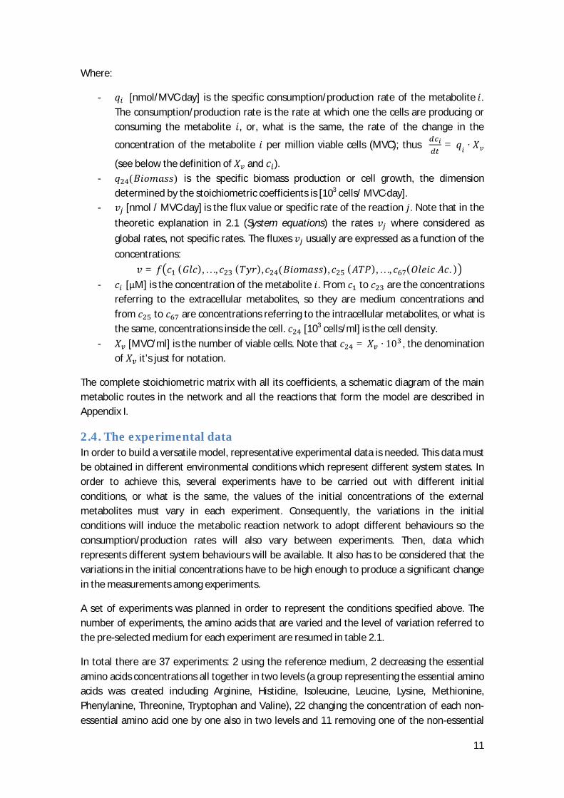
A schematic diagram of the cell density along the time is represented in figure 2.1.

13

Figure 2. 1 Cell density along the time during every experiment

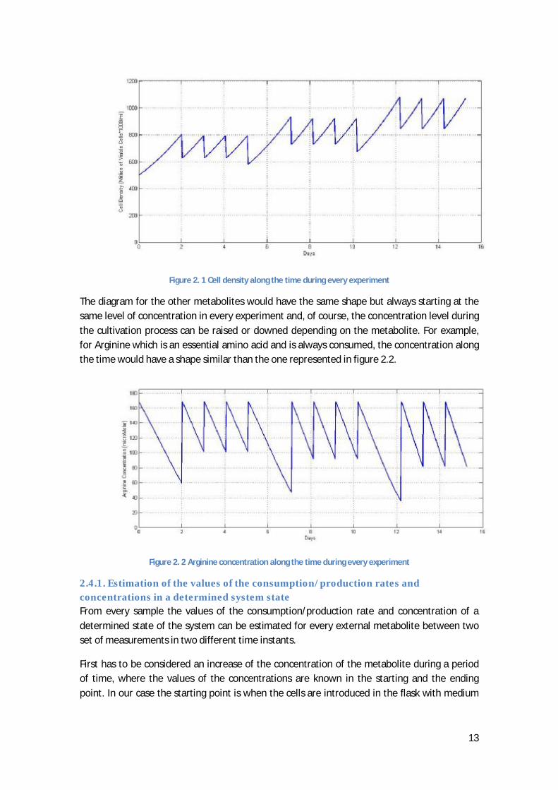
The diagram for the other metabolites would have the same shape but always starting at the same level of concentration in every experiment and, of course, the concentration level during the cultivation process can be raised or downed depending on the metabolite. For example, for Arginine which is an essential amino acid and is always consumed, the concentration along the time would have a shape similar than the one represented in figure 2.2.

Figure 2. 2 Arginine concentration along the time during every experiment

2.4.1. Estimation of the values of the consumption/production rates and concentrations in a determined system state From every sample the values of the consumption/production rate and concentration of a determined state of the system can be estimated for every external metabolite between two set of measurements in two different time instants.

First has to be considered an increase of the concentration of the metabolite during a period of time, where the values of the concentrations are known in the starting and the ending point. In our case the starting point is when the cells are introduced in the flask with medium

14

of known concentration and the ending point is when the samples are taken and the measurements are done after one day.

The method applied to estimate these parameters (consumption/production rates and concentrations for a determined system state) is based in the assumption that the value of the derivative when the concentration of the metabolite is in the middle point of the total increase can be approximated to the change of the concentration divided by the change in time. This is represented in figure 2.3.

Figure 2. 3 Estimation method to obtain and for a determined system state

Thus the specific consumption/production rate for the point where ( ) = (2-14)

can be estimated by the following equation: ( )/ = − ∆ · ( + )2

This method is a simple linearization of the concentration curve suggested by the KTH Division of Bioprocess and is usually used for estimating the consumption rates when doing flux analyses. It is based on the fact that the kinetics for biological systems metabolites usually have an exponential growth but very smooth.

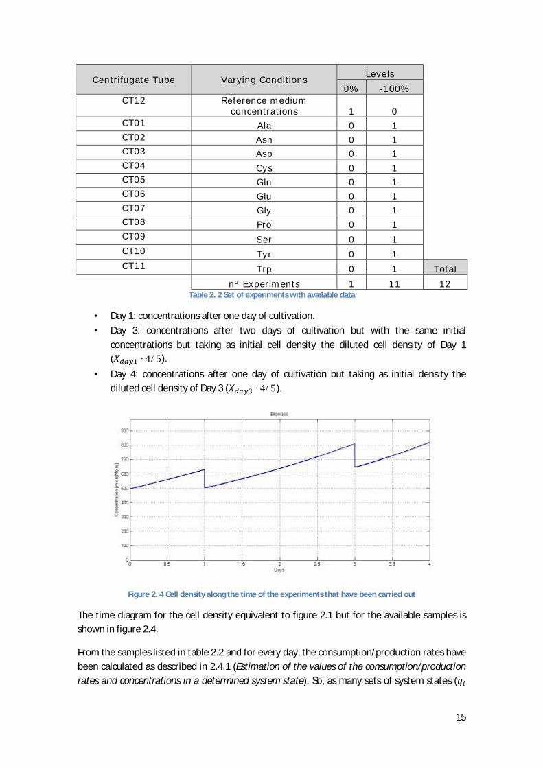
2.4.2. The available experimental data The experiments that have been carried out differ a little from the planned ones. In reality there are sample of 12 different centrifuged tubes (experiments) which ones have different amino acids initial concentrations. The initial values of the concentrations of the centrifuged tube taken as reference (CT12) are shown in table 2.3 and the initial concentration variations respecting to CT12 of the other centrifuged tubes summarized in table 2.2.

There are available samples of the concentrations of the amino acids, glucose, ammonia and lactate of three different days for each of the centrifuged tubes (excepting Day 1 for CT04 and CT08):

(2-15)

15

Centrifugate Tube Varying Conditions Levels 0% -100% CT12 Reference medium

concentrations 1 0 CT01 Ala 0 1 CT02 Asn 0 1 CT03 Asp 0 1 CT04 Cys 0 1 CT05 Gln 0 1 CT06 Glu 0 1 CT07 Gly 0 1 CT08 Pro 0 1 CT09 Ser 0 1 CT10 Tyr 0 1

CT11 Trp 0 1 Total nº Experiments 1 11 12

Table 2. 2 Set of experiments with available data

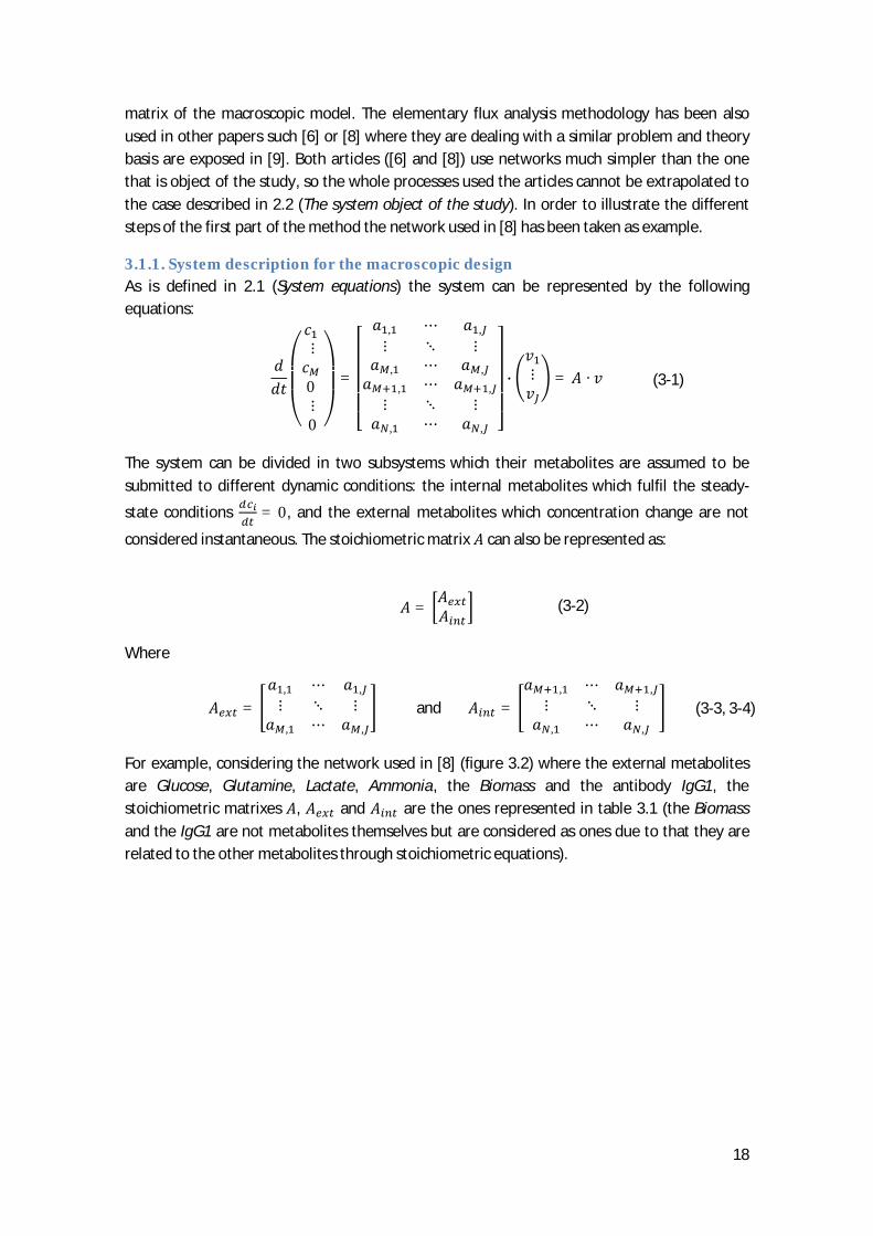
• Day 1: concentrations after one day of cultivation.

• Day 3: concentrations after two days of cultivation but with the same initial concentrations but taking as initial cell density the diluted cell density of Day 1 ( · 4/5).

• Day 4: concentrations after one day of cultivation but taking as initial density the diluted cell density of Day 3 ( · 4/5).

Figure 2. 4 Cell density along the time of the experiments that have been carried out

The time diagram for the cell density equivalent to figure 2.1 but for the available samples is shown in figure 2.4.

From the samples listed in table 2.2 and for every day, the consumption/production rates have been calculated as described in 2.4.1 (Estimation of the values of the consumption/production rates and concentrations in a determined system state). So, as many sets of system states (

16

and ) as samples are obtained. The calculated values for and can be found in Appendix III.

One problem is that in the available experimental data the values of the concentrations of Serine and Asparagine are summed in the same value. The dealing with this problem will be exposed in 5.3.1 (The problem with Serine and Asparagine).

Concentrations in CT12 (µM) Glucose 17500 Lactate 0 NH4 0 Glutamine 4000 Glutamate 258,1 Arginine 1765,3 Histidine 168,6 Isoleucine 455,5 Leucine 682,9 Lysine 542,8 Methionine 127,5 Phenylanine 199,3 Threonine 440,7 Tryptophan 45,2 Valine 607,7 Alanine 204,7 Aspargine+Serine 779,2 Aspartate 174,10 Cysteine 694,0 Glycine 252,1 Proline 402,7 Tyrosine 315,2 Cell density (MVC/ml) 0,5

Table 2. 3 Initial concentrations of the reference medium

17

3. The Modelling Method The method presented here is the main object of the master thesis. The purpose of this methodology is to achieve a dynamical model where only the extracellular metabolites are involved an then simplify it achieving a model as much reduced as possible. The model should be able to predict the consumption/production rates of these metabolites given a determined concentration values.

In this method each cell is considered as a black box device which transforms the extracellular metabolites into other extracellular metabolites. The inputs of the mentioned device will be the extracellular substrates and the outputs the extracellular products. This is represented in figure 3.1 (Note that an extracellular substrate can be at the same time an extracellular product).

Figure 3. 1 The cell as a black box device

In order to calculate this reduced dynamical model, information consisting in two basic elements is needed:

• A pre-defined metabolic network model which should contain the reactions that are wanted to be considered in the system which implies basically the stoichiometric relations between all the compounds in the network or, what is the same, the stoichiometric matrix of the network model.

• Experimental data with samples obtained in different initial conditions describing the different system behaviours that are wanted to be modelled. The format of the data should be the one exposed in 2.4 (The available data); and .

The method consists of two parts:

• The design of the macroscopic model, where a stoichiometric matrix of macroscopic reactions is calculated from the stoichiometric matrix of the pre-defined metabolic network.

• The design of the reduced dynamical model, where a reduced dynamical model which relates the consumption/production of the external metabolites with their concentrations is calculated from the experimental data and the previously calculated stoichiometric matrix of the macroscopic reactions.

3.1. Design of the Macroscopic Stoichiometric Model In this first part of the method a macroscopic model of the system is calculated by using elementary flux analysis. The complexity of the pre-defined stoichiometric matrix and the quantity of extracellular metabolites will determine the size of the resulting stoichiometric

18

matrix of the macroscopic model. The elementary flux analysis methodology has been also used in other papers such [6] or [8] where they are dealing with a similar problem and theory basis are exposed in [9]. Both articles ([6] and [8]) use networks much simpler than the one that is object of the study, so the whole processes used the articles cannot be extrapolated to the case described in 2.2 (The system object of the study). In order to illustrate the different steps of the first part of the method the network used in [8] has been taken as example.

3.1.1. System description for the macroscopic design As is defined in 2.1 (System equations) the system can be represented by the following equations:

⎝⎜⎜⎛ ⋮ 0 ⋮0 ⎠⎟⎟

⎞ =⎣⎢⎢⎢⎢⎡ , ⋯ , ⋮ ⋱ ⋮ , ⋯ , , ⋯ , ⋮ ⋱ ⋮ , ⋯ , ⎦⎥⎥

⎥⎥⎤ ∙ ⋮ = ·

The system can be divided in two subsystems which their metabolites are assumed to be submitted to different dynamic conditions: the internal metabolites which fulfil the steady-

state conditions = 0, and the external metabolites which concentration change are not

considered instantaneous. The stoichiometric matrix can also be represented as:

= Where

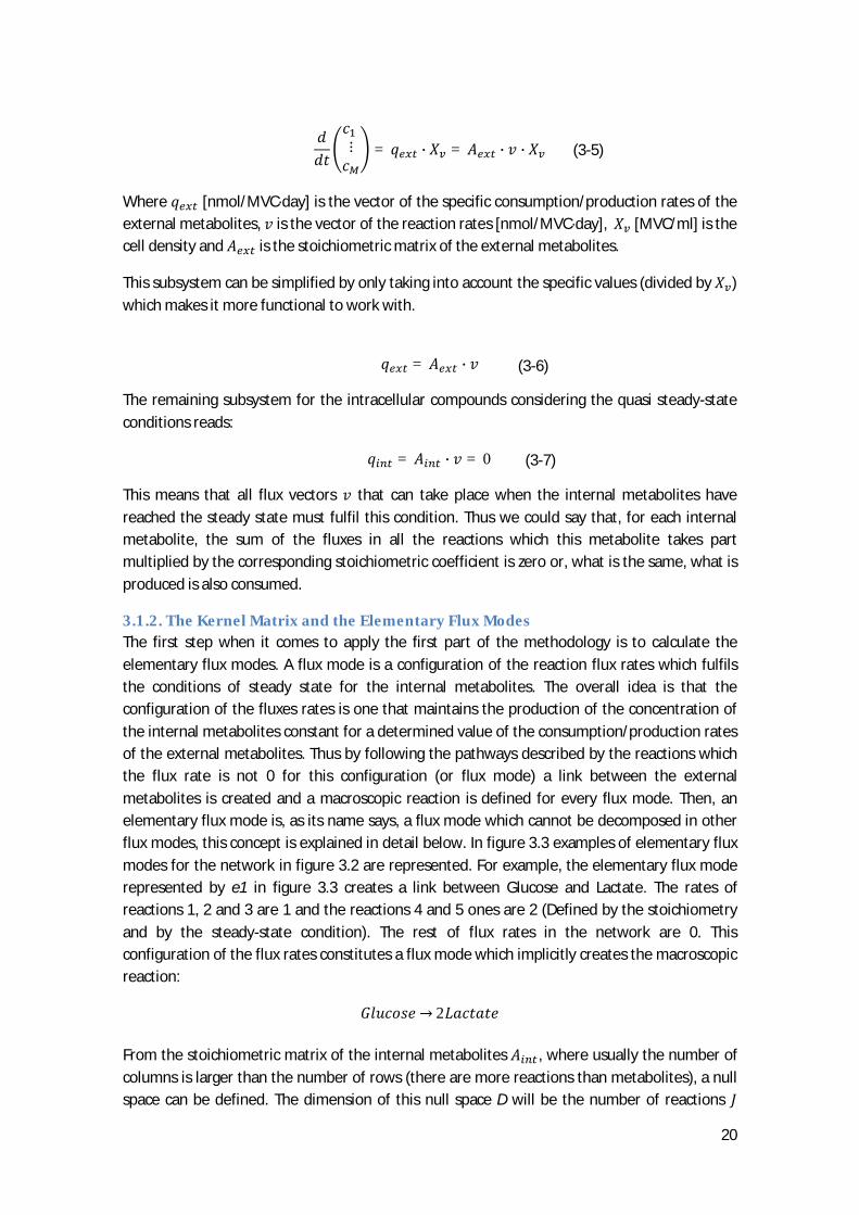
= , ⋯ , ⋮ ⋱ ⋮ , ⋯ , and = , ⋯ , ⋮ ⋱ ⋮ , ⋯ , For example, considering the network used in [8] (figure 3.2) where the external metabolites are Glucose, Glutamine, Lactate, Ammonia, the Biomass and the antibody IgG1, the stoichiometric matrixes , and are the ones represented in table 3.1 (the Biomass and the IgG1 are not metabolites themselves but are considered as ones due to that they are related to the other metabolites through stoichiometric equations).

(3-1)

(3-2)

(3-3, 3-4)

19

Figure 3. 2 Metabolic network of the system used as example [8]

Note that CO2 is not represented in the stoichiometric matrices. This is due to the fact that it is an extracellular metabolite that is only produced and its production rate is not object of the study. As long as it’s always a product it has no effect in the dynamics of the remaining metabolites. Thus it could be included in but the resulting elementary flux modes would be the same ones because they only depend on (see 3.1.2, The Kernel Matrix and the Elementary Flux Modes) and the flux of the macroscopic reactions only depend on the substrates (see 3.2.1, Reaction kinetics modelling).

r1 r2 r3 r4 r5 r6 r7 r8 r9 r10 r11 r12 r13 r14 r15 r16

A

Aext

Glc -1 0 0 0 0 0 0 0 0 0 0 0 0 0 -0,0208 0

Lac 0 0 0 0 1 0 0 0 0 0 0 0 0 0 0 0

NH4 0 0 0 0 0 0 0 0 0 0 0 0 1 1 0 0

Gln 0 0 0 0 0 0 0 0 0 0 0 0 0 -1 -0,0377 -0,0104

Ala 0 0 0 0 0 1 0 0 0 0 0 0 0 0 -0,0133 -0,0112

Biomass 0 0 0 0 0 0 0 0 0 0 0 0 0 0 1 0

IgG1 0 0 0 0 0 0 0 0 0 0 0 0 0 0 0 0

Aint

G6P 1 -1 0 0 0 0 0 0 0 0 0 0 0 0 0 0

DaP 0 1 -1 0 0 0 0 0 0 0 0 0 0 0 0 0

G3P 0 1 1 -1 0 0 0 0 0 0 0 0 0 0 0 0

Pyr 0 0 0 1 -1 -1 -1 0 0 0 0 1 0 0 0 0

AcoA 0 0 0 0 0 0 1 -1 0 0 0 0 0 0 0 0

Cit 0 0 0 0 0 0 0 1 -1 0 0 0 0 0 0 0

α-keto 0 0 0 0 0 1 0 0 1 -1 0 0 1 0 0 0

Mal 0 0 0 0 0 0 0 0 0 1 -1 -1 0 0 0 0

Oxa 0 0 0 0 0 0 0 -1 0 0 1 0 0 0 0 0

Glu 0 0 0 0 0 -1 0 0 0 0 0 0 -1 1 0 0

Table 3. 1 Stoichiometric Matrixes corresponding to figure 3.2

Considering the definitions above, the dynamics of the external metabolites can be described as:

20

⋮ = ∙ = ∙ ∙

Where [nmol/MVC·day] is the vector of the specific consumption/production rates of the external metabolites, is the vector of the reaction rates [nmol/MVC·day], [MVC/ml] is the cell density and is the stoichiometric matrix of the external metabolites.

This subsystem can be simplified by only taking into account the specific values (divided by ) which makes it more functional to work with.

= ∙

The remaining subsystem for the intracellular compounds considering the quasi steady-state conditions reads: = ∙ = 0

This means that all flux vectors that can take place when the internal metabolites have reached the steady state must fulfil this condition. Thus we could say that, for each internal metabolite, the sum of the fluxes in all the reactions which this metabolite takes part multiplied by the corresponding stoichiometric coefficient is zero or, what is the same, what is produced is also consumed.

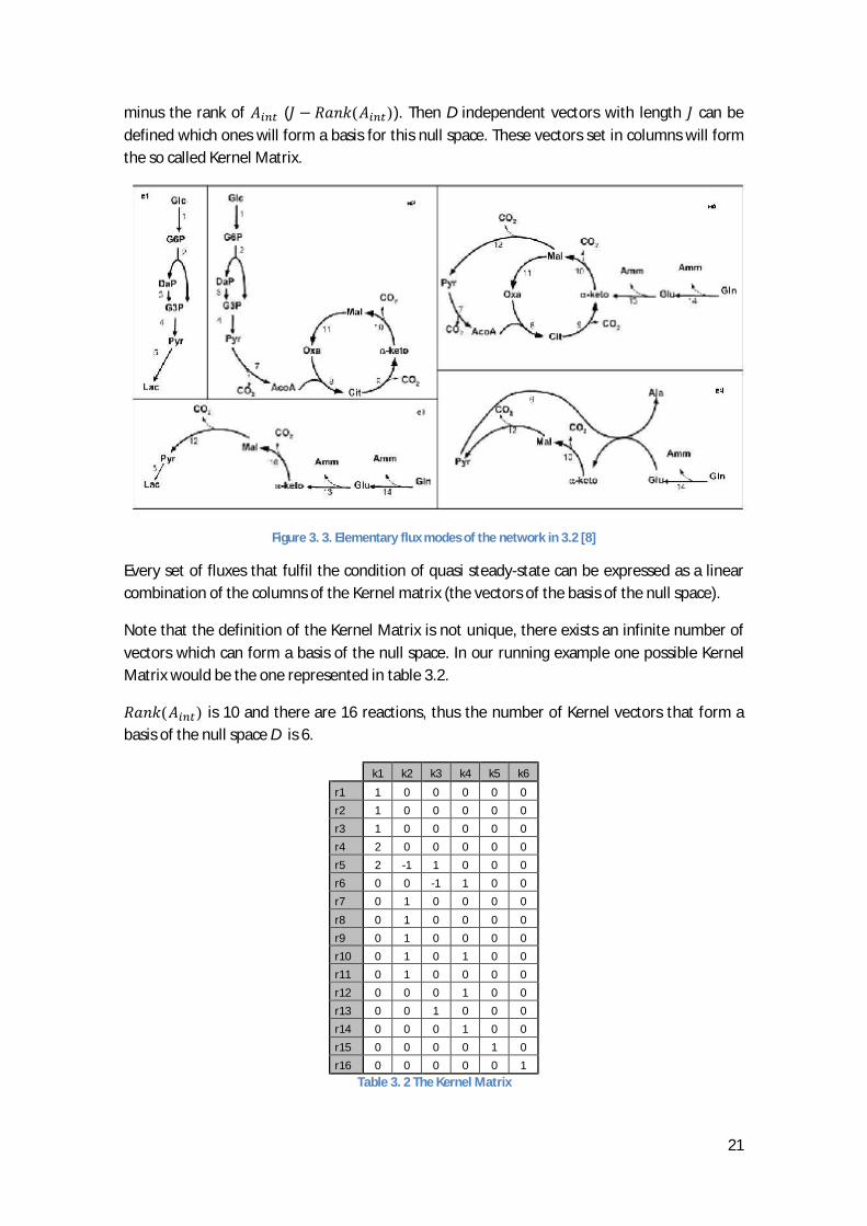
3.1.2. The Kernel Matrix and the Elementary Flux Modes The first step when it comes to apply the first part of the methodology is to calculate the elementary flux modes. A flux mode is a configuration of the reaction flux rates which fulfils the conditions of steady state for the internal metabolites. The overall idea is that the configuration of the fluxes rates is one that maintains the production of the concentration of the internal metabolites constant for a determined value of the consumption/production rates of the external metabolites. Thus by following the pathways described by the reactions which the flux rate is not 0 for this configuration (or flux mode) a link between the external metabolites is created and a macroscopic reaction is defined for every flux mode. Then, an elementary flux mode is, as its name says, a flux mode which cannot be decomposed in other flux modes, this concept is explained in detail below. In figure 3.3 examples of elementary flux modes for the network in figure 3.2 are represented. For example, the elementary flux mode represented by e1 in figure 3.3 creates a link between Glucose and Lactate. The rates of reactions 1, 2 and 3 are 1 and the reactions 4 and 5 ones are 2 (Defined by the stoichiometry and by the steady-state condition). The rest of flux rates in the network are 0. This configuration of the flux rates constitutes a flux mode which implicitly creates the macroscopic reaction: → 2

From the stoichiometric matrix of the internal metabolites , where usually the number of columns is larger than the number of rows (there are more reactions than metabolites), a null space can be defined. The dimension of this null space D will be the number of reactions

(3-5)

(3-6)

(3-7)

21

minus the rank of ( − ( )). Then D independent vectors with length can be defined which ones will form a basis for this null space. These vectors set in columns will form the so called Kernel Matrix.

Figure 3. 3. Elementary flux modes of the network in 3.2 [8]

Every set of fluxes that fulfil the condition of quasi steady-state can be expressed as a linear combination of the columns of the Kernel matrix (the vectors of the basis of the null space).

Note that the definition of the Kernel Matrix is not unique, there exists an infinite number of vectors which can form a basis of the null space. In our running example one possible Kernel Matrix would be the one represented in table 3.2. ( ) is 10 and there are 16 reactions, thus the number of Kernel vectors that form a basis of the null space D is 6.

k1 k2 k3 k4 k5 k6

r1 1 0 0 0 0 0

r2 1 0 0 0 0 0

r3 1 0 0 0 0 0

r4 2 0 0 0 0 0

r5 2 -1 1 0 0 0

r6 0 0 -1 1 0 0

r7 0 1 0 0 0 0

r8 0 1 0 0 0 0

r9 0 1 0 0 0 0

r10 0 1 0 1 0 0

r11 0 1 0 0 0 0

r12 0 0 0 1 0 0

r13 0 0 1 0 0 0

r14 0 0 0 1 0 0

r15 0 0 0 0 1 0

r16 0 0 0 0 0 1

Table 3. 2 The Kernel Matrix

22

If the flux of one reaction is always equal to 0 in all the vectors of the Kernel matrix, this means that the reaction corresponding to this flux is an equilibrium reaction and it will never take place under the quasi steady-state conditions (property 1); the flux of this reactions will be always zero when the intracellular metabolites have reached the steady state. And if the flux values of two or more reactions are the same (or a multiple) in all the vectors of the Kernel matrix, this means that these reactions form an unbranched reaction path; the value of the fluxes for these reactions will be the same (or a multiple) in all the sets of fluxes under the quasi steady-state conditions (property 2).

In the matrix above (table 3.2) it can be seen that reactions 1, 2, 3 and 4 always have the same entries for all the Kernel vectors (or a multiple). This means that it is an unbranched path. Thus reactions 1, 2, 3 and 4 could be simplified for the reaction → 2 (see figure 3.2).

In this case there are no entries in the Kernel vectors that are always zero, thus there are no equilibrium reactions and all the reactions can occur in quasi steady-state conditions.

We can now define a flux mode. A flux mode is a set of flux vectors defined as ( is the number of reactions, 16 in the running example):

= { ∈ | = · ∗; > 0}

Where ∗ fulfil two conditions:

• The steady-state condition; · ∗ = 0.

• The sign restriction condition defined by the reversibility of the reactions. This means that the entries ∗ corresponding to a reaction which is irreversible has to be

positive, so the reactions only occurs in the direction predefined in the stoichiometric matrix.

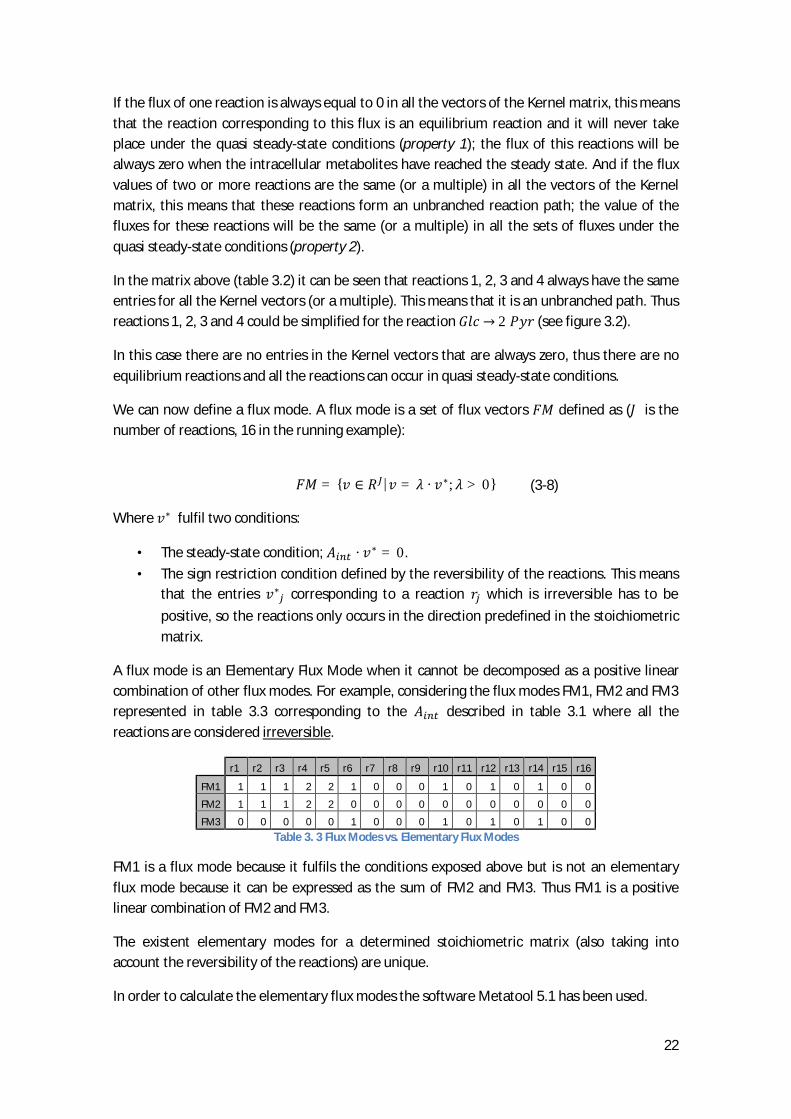
A flux mode is an Elementary Flux Mode when it cannot be decomposed as a positive linear combination of other flux modes. For example, considering the flux modes FM1, FM2 and FM3 represented in table 3.3 corresponding to the described in table 3.1 where all the reactions are considered irreversible.


FM1 1 1 1 2 2 1 0 0 0 1 0 1 0 1 0 0

FM2 1 1 1 2 2 0 0 0 0 0 0 0 0 0 0 0

FM3 0 0 0 0 0 1 0 0 0 1 0 1 0 1 0 0

Table 3. 3 Flux Modes vs. Elementary Flux Modes

FM1 is a flux mode because it fulfils the conditions exposed above but is not an elementary flux mode because it can be expressed as the sum of FM2 and FM3. Thus FM1 is a positive linear combination of FM2 and FM3.

The existent elementary modes for a determined stoichiometric matrix (also taking into account the reversibility of the reactions) are unique.

In order to calculate the elementary flux modes the software Metatool 5.1 has been used.

(3-8)

23

Metatool 5.1 is a software application which can be run in Matlab or GNU Octave and allows us to calculate the elementary flux modes. Just by giving as input the internal metabolites stoichiometric matrix and a vector with length the number of reactions containing logical values which indicates the reversibility of the reactions (1 if irreversible, 0 if reversible), a matrix where the rows correspond to the reactions and the columns to the uniquely defined elementary modes can be calculated. The Metatool syntax and description can be found in [10].

3.1.3. The Metatool procedure By calculating a Kernel matrix for , the first step executed by Metatool is to build a reduced system using the properties 1 & 2 described above in the previous point (3.1.2). First, the columns of the main stoichiometric matrix corresponding to the blocked reactions are removed from the system, and also the rows corresponding to the metabolites that only are involved in these reactions (property 1), the blocked reactions are the equilibrium reactions which their entry is always 0. Using property 2, subsets of reactions that represent the unbranched paths are created.

In the running example there are no blocked reactions and the subsets corresponding to the unbranched paths are:

• Reactions 1, 2, 3 and 4.

• Reactions 7, 8, 9 and 11.

• Reactions 12 and 14.

In the reduced system, these subsets will be represented as a linear combination of their reactions. These linear combinations reduce the number of metabolites, creating zeros in the rows corresponding to these metabolites which are in the middle of the unbranched paths.

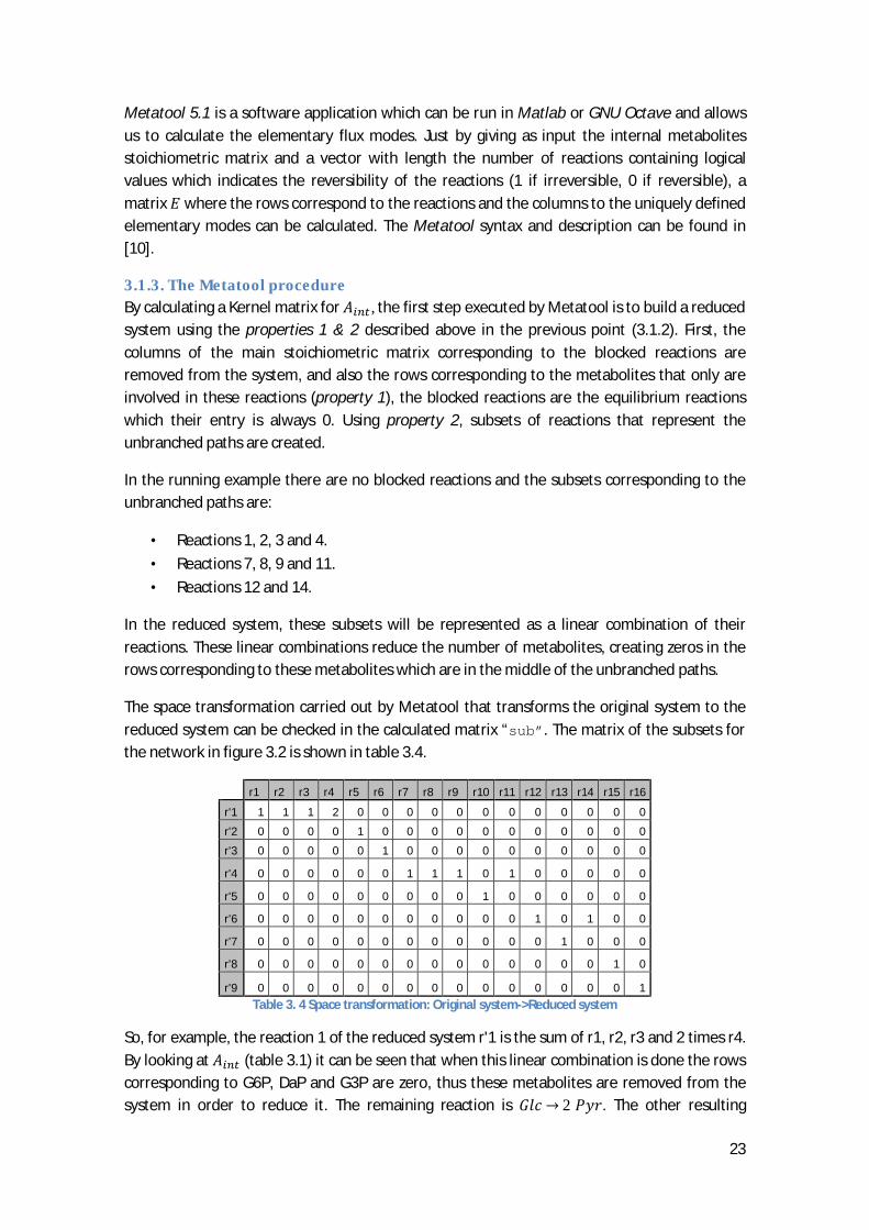
The space transformation carried out by Metatool that transforms the original system to the reduced system can be checked in the calculated matrix “sub”. The matrix of the subsets for the network in figure 3.2 is shown in table 3.4.


r'1 1 1 1 2 0 0 0 0 0 0 0 0 0 0 0 0

r'2 0 0 0 0 1 0 0 0 0 0 0 0 0 0 0 0

r'3 0 0 0 0 0 1 0 0 0 0 0 0 0 0 0 0

r'4 0 0 0 0 0 0 1 1 1 0 1 0 0 0 0 0

r'5 0 0 0 0 0 0 0 0 0 1 0 0 0 0 0 0

r'6 0 0 0 0 0 0 0 0 0 0 0 1 0 1 0 0

r'7 0 0 0 0 0 0 0 0 0 0 0 0 1 0 0 0

r'8 0 0 0 0 0 0 0 0 0 0 0 0 0 0 1 0

r'9 0 0 0 0 0 0 0 0 0 0 0 0 0 0 0 1

Table 3. 4 Space transformation: Original system->Reduced system

So, for example, the reaction 1 of the reduced system r'1 is the sum of r1, r2, r3 and 2 times r4. By looking at (table 3.1) it can be seen that when this linear combination is done the rows corresponding to G6P, DaP and G3P are zero, thus these metabolites are removed from the system in order to reduce it. The remaining reaction is → 2 . The other resulting

24

equations from the subsets are + → + 2 and + → + + . The last subset doesn’t affect to the metabolites reduction but reduce the system by one more reaction.

The metabolites remaining in the reduced system are registered in the vector “rd_met” (table 3.5).

rd_met

4 7 8 10 Table 3. 5 rd_met; the remaining metabolites in the reduced system

So the reduced system only will have the metabolites number 4, 7, 8 and 10 in which are, respectively, Pyr, α-keto, Mal and Glu.

Applying the space transformation specified in table 3.4 and removing the rows that only contain zeros, the reduced system (table 3.6) reads:

r'1 r'2 r'3 r'4 r'5 r'6 r'7 r'8 r'9

Pyr 2 -1 -1 -1 0 1 0 0 0

α-keto 0 0 1 1 -1 0 1 0 0

Mal 0 0 0 -1 1 -1 0 0 0

Glu 0 0 -1 0 0 1 -1 0 0

Table 3. 6 The reduced system

The next step after checking the linear correlation coefficient of the matrix that Metatool executes, is to check which metabolites in are only produced or consumed and if anyone of them takes part in any reversible reaction. If it exists any metabolite that is only produced or consumed (all the stoichiometric coefficients are positive or negative) and it doesn’t take part in any reversible reaction, automatically, all the reactions where this metabolite is involved will never occur in steady state conditions because the only solution of the equation below (the steady-state condition for the metabolite ) is | = 0. Where | is a vector containing the fluxes which corresponds to the reactions where the stoichiometric coefficient of the metabolite , , is different than 0.

, = [ ⋯ ] · = 0

The same procedure is carried out after removing the blocked reactions due to property 1.

For the stoichiometric matrix of the running example in table 3.2 the result of Metatool is the following:

0 metabolites are only produced, 0 are only consumed; 0 metabolites take part in only one reversible reaction; 0 are unused. Removing 0 blocked reactions from subsets 0 metabolites are only produced, 0 are only consumed; 0 metabolites take part in only one reversible reaction; 0 are unused. In this case, there are no blocked reactions and no metabolites that are only produced or consumed. Thus there are no reactions that won’t take place due to the existence of metabolites that are only produced or consumed.

(3-9)

25

Based on the above, Metatool starts doing combinations with the Kernel vectors that fulfil the condition of elementary mode and the irreversibility conditions. Then the elementary flux modes of the reduced model are calculated in the matrix “rd_ems”, let us call it .

The resulting matrix for the running example is represented in table 3.7. In this case there are 7 elementary flux modes.

e1 e2 e3 e4 e5 e6 e7

r'1 1 1 0 0 0 0 0

r'2 2 0 1 0 0 0 0

r'3 0 0 0 1 0 0 0

r'4 0 2 0 0 1 0 0

r'5 0 2 1 1 2 0 0

r'6 0 0 1 1 1 0 0

r'7 0 0 1 0 1 0 0

r'8 0 0 0 0 0 1 0

r'9 0 0 0 0 0 0 1

Table 3. 7 Elementary Flux Modes of the reduced system

The next step is to calculate the matrix containing the elementary flux modes for the original reactions . This step is not done automatically by Metatool, but can be calculated just by undoing the space transformation from the subsets of reactions to the original reactions (multiplying by the subsets matrix transposed; in table 3.4):

= ·

Finally the matrix (table 3.8) for the system in figure 3.2 reads:

e1 e2 e3 e4 e5 e6 e7

r1 1 1 0 0 0 0 0

r2 1 1 0 0 0 0 0

r3 1 1 0 0 0 0 0

r4 2 2 0 0 0 0 0

r5 2 0 1 0 0 0 0

r6 0 0 0 1 0 0 0

r7 0 2 0 0 1 0 0

r8 0 2 0 0 1 0 0

r9 0 2 0 0 1 0 0

r10 0 2 1 1 2 0 0

r11 0 2 0 0 1 0 0

r12 0 0 1 1 1 0 0

r13 0 0 1 0 1 0 0

r14 0 0 1 1 1 0 0

r15 0 0 0 0 0 1 0

r16 0 0 0 0 0 0 1

Table 3. 8 Elementary Flux Modes

The calculated elementary flux modes from e1 to e5 are the ones represented graphically in figure 3.3. The elementary flux modes e6 and e7 are the corresponding to the reactions that

(3-10)

26

don’t involve intracellular metabolites which are the Biomass production from Glucose and the considered amino acids and the IgG1 production from the considered amino acids.

3.1.3.1. Reactions that don’t involve internal metabolites The reactions that don’t involve internal metabolites can be treated independently of the elementary flux modes calculation as long as they are independent of . These reactions are represented in the stoichiometric matrix of the internal metabolites as columns containing only zeros and Metatool automatically calculates an elementary flux mode for each one of these reactions which contains a 1 in the position corresponding to this reaction (see e6 and e7 in table 3.8). It has been found that when these reactions are considered reversible, Metatool don’t calculate the elementary flux mode corresponding to the reversible reaction, what means an elementary flux mode containing a -1 in the position corresponding to the reaction. In order to solve this problem the methodology that has been adopted is to treat independently these reactions just by adding them and the corresponding reversible reactions to the stoichiometric matrix of the macroscopic reactions defined in the next point 3.1.4. This has been taken into account in the implementation process (4.1).

3.1.4. Calculation of the macroscopic reactions stoichiometry Once all the elementary flux modes are calculated we can define the matrix where the columns of it represent the elementary flux modes and it would have the following shape:

= , ⋯ , ⋮ ⋱ ⋮ , ⋯ , Where , is the value of the flux rate of the reaction in the elementary mode and N is the

number of elementary modes which only depends on the characteristics of . For the running example, J would be equal to 16 (there are 16 reactions) and N is equal to 7. According to the definition the matrix will fulfil: ∙ = 0

Then we can create a link between the external metabolites by considering the steady-state in the system. Here, what is considered is that, in quasi steady-state, the only possible values for the fluxes of all the reactions are a linear combination of the elementary flux modes. So the stoichiometric matrix of the macroscopic reactions can be defined as:

= ∙ = ′ , ⋯ ′ , ⋮ ⋱ ⋮ ′ , ⋯ ′ , Every macroscopic reaction corresponds to one elementary flux modes. We could say that a macroscopic reaction is the flux of an elementary flux mode but seen from an extracellular point of view.

In the example exposed previously, the values of the matrix entries are represented in table 3.9.

(3-11)

(3-12)

(3-13)

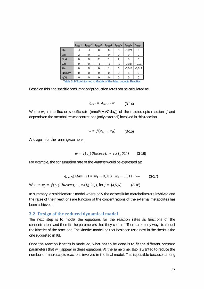
27

rmac1 rmac2 rmac3 rmac4 rmac5 rmac6 rmac7

Glc -1 -1 0 0 0 -0,021 0

Lac 2 0 1 0 0 0 0

NH4 0 0 2 1 2 0 0

Gln 0 0 -1 -1 -1 -0,038 -0,01

Ala 0 0 0 1 0 -0,013 -0,011

Biomass 0 0 0 0 0 1 0

IgG1 0 0 0 0 0 0 0

Table 3. 9 Stoichiometric Matrix of the Macroscopic Reaction

Based on this, the specific consumption/production rates can be calculated as:

= ∙

Where is the flux or specific rate [nmol/(MVC·day)] of the macroscopic reaction and depends on the metabolites concentrations (only external) involved in this reaction.

= ( ,⋯ , )

And again for the running example:

= ( ( ),⋯ , ( 1))

For example, the consumption rate of the Alanine would be expressed as:

, ( ) = − 0,013 · − 0,011 ·

Where = ( ( ),⋯ , ( 1)), for = {4,5,6}

In summary, a stoichiometric model where only the extracellular metabolites are involved and the rates of their reactions are function of the concentrations of the external metabolites has been achieved.

3.2. Design of the reduced dynamical model The next step is to model the equations for the reaction rates as functions of the concentrations and then fit the parameters that they contain. There are many ways to model the kinetics of the reactions. The kinetics modelling that has been used next in the thesis is the one suggested in [6].

Once the reaction kinetics is modelled, what has to be done is to fit the different constant parameters that will appear in these equations. At the same time, also is wanted to reduce the number of macroscopic reactions involved in the final model. This is possible because, among

(3-15)

(3-17)

(3-16)

(3-18)

(3-14)

28

all the elementary flux modes that can occur in the system, not all of them take place, only the ones that are more significant when it comes to fit the data.

In the system which is object of the study where we are dealing with 24 external metabolites, depending on the complexity of the network, there will be hundreds of elementary flux modes (a case completely different of the example used in 3.1). If the number of reactions of the macroscopic model is not reduced, the resulting model will be difficult to deal with. As long as the aim is to find out a model where we could read which reactions are taking place, the macroscopic model has to be reduced.

3.2.1. Reaction kinetics modelling As said before the model that has been used is the suggested in [6]. In order to apply this modelling for the kinetics some assumptions has to be done. The assumptions done next are considering a generalization of all the macroscopic reactions due to the fact that the object of this modelling is to achieve a standard method which can fit in most of the cases:

• All the reactions are considered irreversible, the reversibility of the reactions has been taken into account when the network is defined and the elementary modes are computed.

• Almost all the reactions that take place within the elementary modes are enzyme-catalyzed reactions so the kinetics of the macroscopic reactions which corresponds to the elementary modes also will have enzyme-saturation effect due to the fact that the quantity of enzyme is a finite value. Thus they can be modelled by the Michaelis-Menten dynamics equation [11]:

= · +

Where is the maximal reaction rate when the enzyme is saturated of substrate. is the half-saturation constant which is equal to the concentration level of the substrate when the reaction rate is the half of the maximal in the current reaction. is the reaction rate and is the substrate concentration.

• When a macroscopic reaction has two or more substrates or the stoichiometric coefficient of the substrate is different than 1 (in the equation below the value of the stoichiometric coefficient is represented by ), it is considered that, still under the enzyme-saturation effect, they are subjected to the law of Mass Action [4]. This is actually true; the probability of the reaction to occur is proportional to the probability of collision of the substrates but also during the pathway they will be subjected to enzyme-catalyzed reactions. The kinetics equation for reactions where more than one substrate is involved reads:

= ∏ ∏ , +

Regarding the macroscopic model achieved by computing the elementary modes,

(3-20)

(3-19)

29

⋮ · = ′ , ⋯ ′ , ⋮ ⋱ ⋮ ′ , ⋯ ′ , ∙ ⋮ · = · ·

The resulting standardized kinetic equation for the macroscopic reaction is:

= , ( + ) ,

Where the are the concentrations of the substrates involved in the reaction , is the half-saturation constant of the corresponding metabolite and has the same dimension as the metabolites concentrations [μM]. In this case the saturation is only dependent of the metabolite because what is considered is that the saturation state is reached when there is excess of the current metabolite in the medium. Basically, to simplify the number of parameters, it is assumed that is the same in all reactions for every metabolite. This simplification is assumed in [6] to solve the same problem. Finally, is the maximal rate that

reaction can be produced.

For example, applying these kinetic modelling to the example system used in 3.1 (Design of the Macroscopic Stoichiometric Model), the specific consumption/production rate of Alanine would be modelled as:

, ( )= ( + )− 0,013 · · , ( + ) , · , ( + ) , · , ( + ) , − 0,011 · , ( + ) , · , ( + ) ,

When it comes to apply the proposed methodology the values have to be previously known, this is one of the requirements of the method.

For the system which is object of this study composed by 24 external metabolites described in 2.2 (The system object of the study), as long as the real values are unknown, approximated values have been adopted in order to apply this methodology. The approximated values were suggested by the KTH Division of Bioprocess based on their knowledge about the behaviour of every external metabolite in this kind of systems. These values can be approximated by knowing the limit concentration value for excess of the metabolite in the medium. For example, if it is known that the medium has excess of Glucose, the value (the half saturation constant corresponding to Glucose) has to be small enough to do not have effect for the glucose medium concentrations that we are dealing with. The suggested values are represented in table 3.10.

(3-22)

(3-23)

(3-21)

30

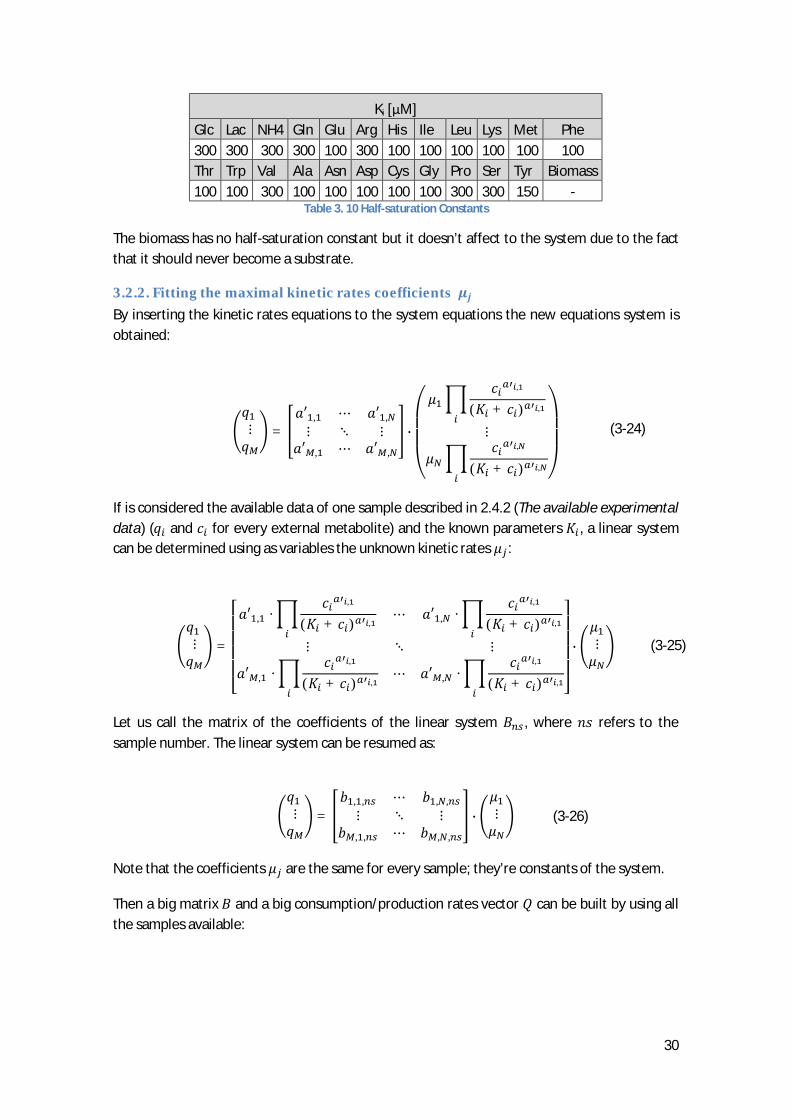
Ki [μM] Glc Lac NH4 Gln Glu Arg His Ile Leu Lys Met Phe 300 300 300 300 100 300 100 100 100 100 100 100 Thr Trp Val Ala Asn Asp Cys Gly Pro Ser Tyr Biomass 100 100 300 100 100 100 100 100 300 300 150 -

Table 3. 10 Half-saturation Constants

The biomass has no half-saturation constant but it doesn’t affect to the system due to the fact that it should never become a substrate.

3.2.2. Fitting the maximal kinetic rates coefficients By inserting the kinetic rates equations to the system equations the new equations system is obtained:

⋮ = ′ , ⋯ ′ , ⋮ ⋱ ⋮ ′ , ⋯ ′ , ∙⎝⎜⎜⎛

, ( + ) , ⋮ , ( + ) , ⎠⎟⎟⎞

If is considered the available data of one sample described in 2.4.2 (The available experimental data) ( and for every external metabolite) and the known parameters , a linear system can be determined using as variables the unknown kinetic rates :

⋮ =⎣⎢⎢⎢⎢⎡ ′ , · , ( + ) , ⋯ ′ , · , ( + ) , ⋮ ⋱ ⋮ ′ , · , ( + ) , ⋯ ′ , · , ( + ) , ⎦⎥⎥

⎥⎥⎤ ∙ ⋮

Let us call the matrix of the coefficients of the linear system , where refers to the sample number. The linear system can be resumed as:

⋮ = , , ⋯ , , ⋮ ⋱ ⋮ , , ⋯ , , ∙ ⋮

Note that the coefficients are the same for every sample; they’re constants of the system.

Then a big matrix and a big consumption/production rates vector can be built by using all the samples available:

(3-26)

(3-25)

(3-24)

31

=⎝⎜⎜⎜⎛ , ⋮ , ⋮ , ⋮ , ⎠⎟

⎟⎟⎞ = ⋮ ∙ ⋮ = ·

is the total number of samples.

Depending on the number of external metabolites, the number of elementary modes or, what is the same, the number of macroscopic reactions and number of samples, this will be an underdetermined, determined or over determined system. This depends, basically, on how the initial network is defined which determine the number of elementary modes and the number of available samples.

In order to determine the values of the maximal kinetic rates , a non-negative least-squares

algorithm is adopted. The following objective function has to be optimized:

= min ‖ · − ‖ ; ℎ ≥ 0

has to be higher or equal than 0 because, as said before, the macroscopic reactions are irreversible, and the only pathways that are considered are the ones corresponding to elementary modes that have been computed taking into account the reversibility of the reactions of the original network.

To solve the non-negative least-squares problem the function lsqnonneg of the Matlab Optimization Tool has been used. By entering the matrix and the vector , it returns the optimal values of and also the minimized value .

The function lsqnonneg uses an algorithm which is based on the dual vector “lambda” associated to the vectors that are in the basis in every step of the algorithm. In every step the vector in the basis with a higher lambda value associated is removed and a new possible candidate enters in the basis of the possible optimal solution. The values of the vector lambda change when the vectors in the basis are also changed. The algorithm is stopped when all the values of lambda are lower than zero. A detailed explanation of the used algorithm can be found in [12].

In order to assure an optimal solution for , the system has to be overdetermined which is the main condition when using least squares methodologies and it’s a requirement for using the function lsqnonneg [13], or what is the same, the matrix has to have more rows than columns. This implies the following condition:

· >

Where is the number of external metabolites, is the number of samples and is the number of macroscopic reactions or elementary flux modes.

(3-27)

(3-29)

(3-28)

32

If this condition is not fulfilled, it cannot be assured that the result will be the optimum because the algorithm of the Matlab function lsqnonneg would be working out of the specifications imposed. However, the obtained result will probably be optimized in some degree due to the fact that the used algorithm is based on the dual vector “lambda” specified above (see [12]), and it will be stopped when all the values in the vector lambda are lower than zero.

Moreover, it could be that the optimal solution is not a point, but a straight line, a plane or a higher dimension set in the -space (dimension of the vector ). In this case, we could say that there is more than one solution for the values in . But as long as we are trying to find the values that fit better the data, anyone of the optimal solutions will be as good as any other configuration of inside the optimal solution set. Then, in this case, the vector calculated directly by lsqnonneg is the one that will be considered the optimal solution.

The usual solution, if is very large, is that most of the will be zero. Regarding this, a

reduced model containing only the macroscopic reactions that the corresponding maximal kinetic rate is higher than 0 can be obtained. As more 0 are on more reduced will be the

model.

If the chosen network configuration can explain all the variations in the data, and the measured values of the data are correct, a good model should be obtained. The model is basically defined by a reduced stoichiometric matrix for the macroscopic reactions , ,

the corresponding maximal kinetic rates to these reactions and a vector containing the values of the half-saturation constants for every external metabolite.

33

4. Implementation In this section are presented the tools that have been developed in order to calculate a dynamical model for a metabolic network following the methodology described in 3 (The Method). All the functions have been implemented in Matlab and their corresponding codes can be found in Appendix VI.

The implemented functions are divided in two groups:

• Method Tools; the functions that calculate the model itself ( , , and extra

information).

• Result Tools; the functions used to predict consumption/production rates and to plot the results.

Next, a brief description of every function specifying the inputs, outputs and the process is presented.

4.1. Method tools calcAmac

Calculates the stoichiometric matrix of the macroscopic reactions specified in 3.1 (Design of the Macroscopic Model). Where Aext is the stoichiometric matrix of the external metabolites,

Aint is the stoichiometric matrix of the internal metabolites and irrev is a row vector with

length equal to the number of reactions which describes the reversibility of the reactions; 1 if the reaction is irreversible and 0 if it is reversible.

Syntax

[Amac] = calcAmac(Aext,Aint,irrev) [Amac,EM] = calcAmac(Aext,Aint,irrev) [Amac,EM,nmodes] = calcAmac(Aext,Aint,irrev) [Amac,EM,nmodes,externalreactions] = calcAmac(Aext,Aint,irrev)

Description

[Amac] = calcAmac(Aext,Aint,irrev)returns the stoichiometric matrix of the macroscopic reactions corresponding to the elementary flux modes (including also the reactions which only implies external metabolites). [Amac,EM] = calcAmac(Aext,Aint,irrev)returns the matrix with all the

elementary flux modes which contains the flux value for every reaction in every possible elementary flux mode. [Amac,EM,nmodes]= calcAmac(Aext,Aint,irrev)returns the number of elementary flux modes. [Amac,EM,nmodes,externalreactions] = calcAmac(Aext,Aint,irrev) returns a vector with the numbers of the reactions that only involve external metabolites.

Algorithm

34

First, the reactions are divided in two groups: reactions where internal metabolites are involved and reactions where only external metabolites are involved (this implies two Aext, two Aint and two irrev put in two struct variables). This division is done because, as

explained in 3.1.3.1 (Reactions that don’t involve internal metabolites), for those reactions where only are implied external metabolites, Metatool don’t calculate the reversible reaction if it should be. After they are separated Metatool is used to calculate the elementary flux modes of the reactions in the first group and next the macroscopic reactions stoichiometric matrix. Then the matrix of the elementary flux modes and the macroscopic stoichiometric matrix of the second group are calculated. The two macroscopic matrixes are put together in a way that the macroscopic reactions corresponding to the reactions that only imply external metabolites are found in the last columns. Finally the matrix of the elementary modes EM is calculated mixing the elementary modes of the two groups and rearranging the rows of the reactions.

Notes

A condition that must be fulfilled is that the number of columns of Aext must be equal to the number of columns of Aint and also equal to the length of the vector irrev. The program

can also work with systems where all the reactions involve internal metabolites as well as systems that only involve external metabolites.

calcmus

This function calculates the values of the estimated maximal kinetic rates (MU) of all the

reactions in the stoichiometric matrix of the macroscopic reactions Amac using a set of data

samples described by C (matrix containing the concentrations; rows metabolites, columns

number of sample) and Q (matrix containing the consumption/production rates; rows

metabolites, columns number of sample) and a row vector K with length equal to the number of metabolites containing the values of the half-saturation constants corresponding to every number of metabolite. The algorithm used is a variation of the one described in 3.2 (Fitting the maximal kinetic rates µj); the new concepts add to this algorithm and their justification are exposed in 5.5 (The new objective function).

Syntax

[MU]=calcmus(A,Q,C,K) [MU,error]=calcmus(A,Q,C,K)

Description

[MU]=calcmus(A,Q,C,K)returns a column vector containing the calculated maximal kinetic rate for every macroscopic reaction. [MU,error]=calcmus(A,Q,C,K)returns the value of the 2-norm of the residual

norm(Q-B*MU).

Algorithm

35

First the matrix of the normalized consumption/production rates Qnorm* described in 5.5

(The new objective function) is calculated from Q. The columns of the matrixes Qnorm and C

are put in two column vectors Qtot and Ctot. Then the coefficients of the matrix *

(named B in the code) are calculated for every macroscopic reaction, sample and metabolite. Finally the Matlab function lsqnoneng calculates the MU vector and the squared 2-norm

using the matrix B and the vector Qnorm.

*See 5.4 (Results for the new network) and 5.5 (The new objective function) for the definition of the variables that are not described in 3.2 (Fitting the maximal kinetic rates µj).

Notes

The number of rows in Amac, Q and C must be equal and also equal to the length of K. The

samples must have the same order in the columns of Q and C. In order to assure an optimal

solution, the number of rows multiplied by the number of columns of Q must be higher than the number of columns in Amac.

calcredsys

This function calculates the reduced system from a macroscopic reactions stoichiometric matrix A and its corresponding vector of the maximal kinetic rates MU.

Syntax

[Ared,MUred]=calcredsys(A,MU)

Description

[Ared,MUred]=calcredsys(A,MU)returns the stoichiometric matrix of the reduced

system Ared and the vector of the maximal kinetic corresponding to the reactions of the reduced system MUred.

Algorithm

This function basically removes the reactions from A that its kinetic rate is 0 and the entries in

MU that are zero. Then it saves them into the new variables Ared and MUred.

findmodel

This function is a combination of the three explained above. From the inputs listed next it calculates directly the reduced system consisting in Ared and MUred.

o Aext is the stoichiometric matrix of the external metabolites o Aint is the stoichiometric matrix of the internal metabolites

o Irrev is a vector with length equal to the number of reactions which

contains a 0 if the reaction is reversible and a 1 if it isn’t. o Q is a matrix containing in every , the value of the specific

consumption/production rates of the metabolite in the sample .

36

o C is a matrix containing in every , the value of the metabolite in the

sample . o K is a vector with length equal to the number of metabolites containing the

values of the half saturation constants.

Syntax

[Ared,MUred]=findmodel(Aext,Aint,irrev,Q,C,K) [Ared,MUred,error]=findmodel(Aext,Aint,irrev,Q,C,K) [Ared,MUred,error,Amac,MU]=findmodel(Aext,Aint,irrev,Q,C,K) [Ared,MUred,error,Amac,MU,EM]=findmodel(Aext,Aint,irrev,Q,C,K) [Ared,MUred,error,Amac,MU,EM,nmodes]=findmodel(Aext,Aint,irrev,Q,C,K) [Ared,MUred,error,Amac,MU,EM,nmodes,externalreactions]=findmodel(Aext,Aint,irrev,Q,C,K) Description

[Ared,MUred]=findmodel(Aext,Aint,irrev,Q,C,K) returns the stoichiometric

matrix of the reduced system and its corresponding maximal kinetic rates. [Ared,MUred,error]=findmodel(Aext,Aint,irrev,Q,C,K) returns the value of the 2-norm of the residual norm(Q-B*MU). [Ared,MUred,error,Amac,MU]=findmodel(Aext,Aint,irrev,Q,C,K)returns the macroscopic reactions stoichiometric matrix corresponding to all the elementary flux modes and its corresponding maximal kinetic rates. [Ared,MUred,error,Amac,MU,EM]=findmodel(Aext,Aint,irrev,Q,C,K) returns the matrix with all the elementary flux modes. [Ared,MUred,error,Amac,MU,EM,nmodes]=findmodel(Aext,Aint,irrev,Q,C,K) returns the number of elementary flux modes. [Ared,MUred,error,Amac,MU,EM,nmodes,externalreactions]=findmodel(Aext,Aint,irrev,Q,C,K) returns a vector with the numbers of the reactions that only

involve external metabolites.

Algorithm

The algorithm of this function is the consecution of the algorithms of the three functions above which constitutes the whole method exposed in 3 (The Method).

Notes

If the condition · > is not fulfilled, the program will give a warning message specifying it.

All the dimension conditions of the three functions exposed above must be also fulfilled. Furthermore the number of external metabolites in Aext must be the same than the ones

contained in the data inputs Q and C.

37

In the code exposed in Appendix VI, line 6 and 7 are added for the special case presented in the results (5, Results and Analysis) due to the problem with the measurements exposed in 5.3.1 (The problem with Serine and Asparagine).

4.2. Result tools calcrates

This function gives a prediction of the production/consumption rates of every external metabolite by giving the following inputs:

o A is the stoichiometric matrix of the external metabolites

o MU is a column vector with length equal to the number of macroscopic

reactions in A containing its corresponding values of the kinetic rates. o K is a vector with length equal to the number of metabolites containing the

values of the half saturation constants. o C is a matrix containing the concentration values of the external metabolites

(rows) in every system state (columns) that is wanted to be predicted the consumption/production rates.

Syntax

Q=calcrates(A,MU,C,K) Description

Q=calcrates(A,MU,C,K) returns a matrix containing the predicted value of the consumption/production rate of every external metabolite (rows) for every system state (every column corresponds to the state in the same column in C).

Algorithm

The algorithm calculates the reaction rates from the kinetic model in 3.2.1 (Reaction kinetics modelling) and then multiplies the vector of the reaction rates by the stoichiometric matrix as follows:

⋮ = , ⋯ , ⋮ ⋱ ⋮ , ⋯ , ∙⎝⎜⎜⎛

, ( + ) , ⋮ , ( + ) , ⎠⎟⎟⎞

The calculation above is carried out for every column in C.

plotQ

(4-1)

38

This function compares a set of calculated values of the consumption/production rates using the function calcrates (Qcalc) with the calculated values directly from the data (Q) corresponding to the same concentration values that have been used in calcrates.

Syntax

null=plotQ(Q,Qcalc,experiments,plotcol) Description

null=plotQ(Q,Qcalc,experiments,plotcol)plots in every subplot the values of the consumption/production rates calculated directly from the data (in blue) and the values of the consumption/production rates calculated with the function calcrates (in red) (Y axis) for

every external metabolite associated to a number (X axis). All the subplots are plotted in the same figure and it has as many subplots as columns in Q or Qcalc. plotcol determines the

number of columns of subplots in the figure and experiments is a character matrix

containing in each row the name of the samples that are being plotted. The names must have the same length. See examples in figures 5.2 and 5.4.

plotQ2

This function does the same comparison than plotQ but removing the three first metabolites. This function is only useful in the case treated in the results (5, Results and Analysis) where the three first metabolites are Glucose, Lactate and Ammonia which have consumption/production rate average values much higher than the other metabolites. The aim of this function is to have a better perspective when it comes to compare the metabolites.

The inputs and their functionality are the same than plotQ.

Syntax

null=plotQ2(Q,Qcalc,experiments,plotcol)

plotQnorm

This function compares the normalized values of a set of calculated values of the consumption/production rates using the function calcrates (Qcalc) with the calculated

values directly from the data (Q) corresponding to the same concentration values that have

been used in calcrates. The normalized values for every sample ( ) and metabolite ( ) and for Q and Qcalc are calculated using the following equations ( is the average of the consumption/production rates calculated directly from the measurements):

, = ,

, , = , (4-3)

(4-2)

39

Note that the used average value is in both cases the one corresponding to the values calculated directly from the measurements.

See 5.4 (Results for the new network) for details.

Syntax

null=plotQnorm(Q,Qcalc,experiments,plotcol) Description

null=plotQnorm(Q,Qcalc,experiments,plotcol)plots in every subplot the

values of the normalized consumption/production rates calculated directly from the data (in blue) and the normalized values of the consumption/production rates calculated with the function calcrates (in red) (Y axis) for every external metabolite associated to a number (X

axis). All the subplots are plotted in the same figure and it has as many subplots as columns in Q or Qcalc. plotcol determines the number of columns of subplots in the figure and experiments is a character matrix containing in each row the name of the samples that are

being plotted. The names must have the same length.

ploterrors

This function plots the relative error calculated from the calculated values of the consumption/production rates using the function calcrates (Qcalc) with the calculated

values directly from the data (Q) corresponding to the same concentration values that have

been used in calcrates taking as real values the ones in Q. The equation used to calculate

the error for every sample ( ) and metabolite ( ) reads:

, = , − , , = , − ,

See 5.4 (Results for the new network) for details.

Syntax

null=ploterrors(Q,Qcalc,experiments,plotcol) Description

null=ploterrors(Q,Qcalc,experiments,plotcol)plots in every subplot the values of the normalized error (Y axis) for every external metabolite associated to a number (X axis). All the subplots are plotted in the same figure and it has as many subplots as columns in Q or Qcalc. plotcol determines the number of columns of subplots in the figure and experiments is a character matrix containing in each row the name of the samples that are being plotted. The names must have the same length. plotevery

This function executes the four plotting functions described above.

(4-4)

40

Syntax

null=plotevery(Q,Qcalc,experiments,plotcol,maxplots) Description

null=plotevery(Q,Qcalc,experiments,plotcol,maxplots)executes the four functions described above but in as many figures per function as the number of columns in Q (number of samples) divided by maxplots. The value maxplots limits the number of subplots per figure. plotcol determines the number of columns of subplots in one figure and experiments is a character matrix containing in each row the name of the samples that are being plotted. The names must have the same length. plotQmet

This function plots in the same plot the different consumption/production rates (the one calculated directly from the measurements and the one calculated with the function calcrates) for every sample (columns in Q) and for the same metabolite (rows in Q). This allows us to compare the change in the different samples and if the rates calculated with the function calcrates follow the same patrons than the other ones. Syntax

null=plotQmet(Q,Qcalc,metabolites,plotcol) Description

null=plotQmet(Q,Qcalc,metabolites,plotcol) plots in every subplot the values of the consumption/production rates calculated directly from the data (in blue) and the values of the consumption/production rates calculated with the function calcrates (in red) (Y axis) for every sample associated to a number (X axis). All the subplots are plotted in the same figure and it has as many subplots as rows in Q or Qcalc. plotcol determines the number

of columns of subplots in the figure and metabolites is a character matrix containing in each row the name of the every metabolite that is being plotted. The names must have the same length.

ploteverymet

This function executes the function plotQmet but with the option to plot the subplots corresponding to the metabolites in different figures. Syntax

null=ploteverymet(Q,Qcalc,metabolites,plotcol,maxplots) Description

null=ploteverymet(Q,Qcalc,metabolites,plotcol,maxplots)executes the

function plotQmet but in as many figures per function as the number of rows in Q

41

(number of metabolites) divided by maxplots. The value maxplots limits the number of

subplots per figure. plotcol determines the number of columns of subplots in one figure

and metabolites is a character matrix containing in each row the name of the samples

that are being plotted. The names must have the same length.

42

5. Results and analysis

5.1. Results for the available network By applying the method to the stoichiometric model described in 2.3 (The available network) as starting point, the elementary flux modes have been directly calculated using Metatool 5.1 in Matlab.

The first response that we obtained when applying this is the following:

2 metabolites are only produced, 3 are only consumed; 0 metabolites take part in only one reversible reaction; 0 are unused. Removing 9 blocked reactions from subsets 2 metabolites are only produced, 4 are only consumed; 0 metabolites take part in only one reversible reaction; 0 are unused.

k1 k2 k3 k4 k5 k6 k7 k8 k9 k10 k11 k12

r1 0 0 0 0,5 0 0 0 0 0 0 0 0 r2 0 1 -0,5 1,5 -10,5 27 65 0 32,5 -35,5 -14 5 r3 1 -1 -0,5 0,5 -11,5 24 62 3 28,5 -28,5 -15 7 r4 0 0 0 0 0 1 0 -1 0 0 -1 0 r5 0 0 0 1 -12 12 42 9 12 -12 -12 9 r6 0 0 0 0 0 0 0 0 -1 0 0 0 r7 0 0 -1 1 -21 51 127 3 61 -65 -29 12 r8 0 0 0 0 0 0 0 0 0 0 0 0 r9 0 0 0 0 5 -10 -26 -1 -12 13 6 -2 r10 0 0 0 0 -1 4 8 -3 6 -6 -1 0 r11 1 0 0 0 0 0 0 0 0 0 0 0 r12 0 0 0 0 1 -6 -12 2 -8 9 2 0 r13 0 -1 -0,5 0,5 -9,5 21 53 2 25,5 -26,5 -12 6 r14 0 1 0 0 0 0 0 0 0 0 0 0 r15 0 0 1 0 0 0 0 0 0 0 0 0 r16 0 0 0 0 -4 2 12 6 2 -2 -3 2 r17 0 0 0 0 0 0 -1 1 0 0 1 0 r18 0 0 0 0 2 0 -4 -4 0 0 0 -1 r19 0 0 0 0 4 -4 -14 -3 -4 4 4 -2 r20 0 0 0 0 -1 9 17 -4 11 -11 -4 0 r21 0 0 0 0 0 -3 -5 2 -3 3 2 0 r22 0 0 0 0 0 0 0 0 -1 1 -1 0 r23 0 0 0 0 0 1 2 -2 1 -1 -1 0 r24 0 0 0 0 0 1 0 -1 0 0 -1 0 r25 0 0 0 0 1 0 0 0 0 0 0 0 r26 0 0 0 0 0 0 0 0 0 0 0 0 r27 0 0 0 0 0 0 0 0 0 0 0 0 r28 0 0 0 0 0 0 0 0 0 0 0 0 r29 0 0 0 0 0 0 0 0 0 0 0 0 r30 0 0 0 0,5 0 0 0 0 0 0 0 0 r31 0 0 0 1 0 0 0 0 0 0 0 0 r32 0 0 0 0 0 0 0 0 0 0 0 0 r33 0 0 0 0 1 0 0 0 0 0 0 0 r34 0 0 0 0 0 0 0 1 0 0 0 0 r35 0 0 0 0 0 0 0 1 0 0 0 0 r36 0 0 0 0 0 1 0 0 0 0 0 0 r37 0 0 0 0 0 0 1 0 0 0 0 0 r38 0 0 0 0 0 0 0 1 0 0 1 0 r39 0 0 0 0 0 0 0 1 0 0 0 0 r40 0 0 0 0 0 0 0 0 1 0 0 0 r41 0 0 0 0 0 0 0 0 0 1 0 0 r42 0 0 0 0 0 0 0 0 0 0 0 0 r43 0 0 0 0 0 0 0 0 0 0 0 0 r44 0 0 0 0 0 0 0 0 0 0 1 0 r45 0 0 0 0 0 0 0 0 0 0 0 1 r46 0 0 0 0 0 0 0 0 0 0 0 0

Table 5. 1 The kernel matrix of the matrix described in Appendix I. Observation: as explained in 3.1.2, we can see in the Kernel matrix calculated by Metatool that the number of vectors is the number of reactions minus the rank of (previously calculated); − = .

Matlab indicates us that from a beginning 2 metabolites are only produced and 3 metabolites are only consumed (all the stoichiometric coefficients corresponding to these metabolites have the same sign). This means that the reactions where these metabolites are involved will never

43

take place unless one of them is reversible (∑ · = 0 for an internal metabolite in order to

reach the steady-state, if all the coefficients for this metabolites have the same sign the

only solution to the equation is = 0,∀ ). Then the reactions where the metabolite of the

reversible reaction is involved will be unblocked, but the flux in this reaction only could have negative values. If we have a look at (see Appendix I) we can see that the metabolites FAD and mFADH are only produced and FADH, mFAD and O2 are only consumed. None of them is involved in reactions number 5 and 14 (the reversible ones), so the reactions number 16, 17, 18, 20, 21, 22, 23, 27, 38, 43, 45 and 46 will never occur.

Furthermore, it says that 9 reactions are blocked, what means that the Kernel matrix (table 5.1) of always have zeros in the rows corresponding to these reactions, so even if all the reactions where reversible they would never occur (property 1, in 3.1.2, The Kernel Matrix and the Elementary Flux Modes). We can identify these reactions by looking at the Kernel matrix (table 5.1) calculated by Metatool or also the vector blocked_react gives us directly the numbers of these reactions. The blocked reactions are number 8, 26, 27, 28, 29, 32, 42, 43 and 46.

Elementary Flux Modes

e1 e2 e3 e4 e5 e6 r1 0,5 0 1,3333 0,5 0,25 0,5 r2 2 0 4 1 0 0 r3 0 1 1,3333 0 1 1 r4 0 0 0 0 0 0 r5 1 0 2,6667 1 0,5 1 r6 0 0 0 0 0 0 r7 1 0 2,6667 0 0,5 0 r8 0 0 0 0 0 0 r9 0 0 0 0 0 0 r10 0 0 0 0 0 0 r11 0 1 0 0 0 0 r12 0 0 0 0 0 0 r13 0 0 1,3333 0 1 1 r14 0,5 0 0 0 -0,75 -1 r15 0 0 0 1 0 1 r16 0 0 0 0 0 0 r17 0 0 0 0 0 0 r18 0 0 0 0 0 0 r19 0 0 0 0 0 0 r20 0 0 0 0 0 0 Amac r21 0 0 0 0 0 0 r22 0 0 0 0 0 0

a'1 a'2 a'3 a'4 a'5 a'6 r23 0 0 0 0 0 0

c1 -0,5 0 -1,333 -0,5 -0,25 -0,5

r24 0 0 0 0 0 0

c2 2 0 4 1 0 0 r25 0 0 0 0 0 0

c3 0 0 0 0 0 0

r26 0 0 0 0 0 0

c4 1 0 2,6667 1 0,5 1 r27 0 0 0 0 0 0

c5 -0,5 0 -1,333 -1 -0,25 -1

r28 0 0 0 0 0 0

c6 0 0 -1,333 0 -1 -1 r29 0 0 0 0 0 0

c7 0 0 0 0 0 0

r30 0,5 0 1,3333 0,5 0,25 0,5

c8 0 0 0 0 0 0 r31 1 0 2,6667 1 0,5 1

c9 0 0 0 0 0 0

r32 0 0 0 0 0 0

c10 0 0 0 0 0 0 r33 0 0 0 0 0 0

c11 0 0 0 0 0 0

r34 0 0 0 0 0 0

c12 0 0 0 0 0 0 r35 0 0 0 0 0 0

c13 0 0 0 0 0 0

r36 0 0 0 0 0 0

c14 0 0 0 0 0 0 r37 0 0 0 0 0 0

c15 0 0 0 0 0 0

r38 0 0 0 0 0 0

c16 0 1 1,3333 0 1 1 r39 0 0 0 0 0 0

c17 0 0 0 -1 0 -1

r40 0 0 0 0 0 0

c18 0 0 0 1 0 1 r41 0 0 0 0 0 0

c19 0 -1 0 0 0 0

r42 0 0 0 0 0 0

c20 0 0 0 0 0 0 r43 0 0 0 0 0 0

c21 -0,5 0 0 0 0,75 1

r44 0 0 0 0 0 0

c22 -1 0 -2,667 0 -0,5 0 r45 0 0 0 0 0 0

c23 0 0 0 0 0 0

r46 0 0 0 0 0 0

c24 0 0 0 0 0 0

Table 5. 2 Elementary flux modes (left) and the macroscopic reactions stoichiometric matrix (right)

Automatically, when these reactions are removed, also the metabolites mNAD, mNADH and Oxal are only produced or consumed (taking into account also the previous metabolites which

44

were only produced/consumed, there are 2 produced only and 4 consumed only; mFADH and mFAD are removed of the system because only participate in reaction 46 that has been removed). So the reactions number 4, 6, 10, 16, 17, 18, 19, 21, 23, 33, 35, 36, 39 and 40 will never take place neither. This will produce a chain of blocks which won’t let a lot of reactions occur assuming the quasi steady-state conditions.

Finally after taking into account the reversibility of the reactions the matrixes and are calculated (Table 5.2). All the reaction that cannot occur in quasi steady-state can be identified in the matrix ; they are the reactions which their corresponding row in the matrix is equal to 0.

Thus, the macroscopic reactions corresponding to the 6 elementary flux modes are:

1. + + + 2 → 4 + 2

2. →

3. + + + 2 → 3 + 2 + 1

4. + 2 + 2 → 2 + 2 + 2

5. + + 4 + 2 → 2 + 4 + 3

6. + 2 + 2 + 2 → 2 + 2 + 2 + 2

And finally the vector of the flux rates of these reactions reads:

1. = · · · ( )( )( )( )

2. = ( ) 3. = · · · ( )( )( )( )

4. = · · ( )( ) ( )

5. = · · · ( )( )( ) ( ) 6. = · · · ( )( ) ( ) ( )

Up on now by applying the second part of the method, the maximal kinetic rates of the macroscopic reactions should be calculated. But before going further into the method, the results that have been obtained should be analysed.

5.1.1. Results analysis First the results can be analysed from an external point of view, considering the correspondence with the data obtained and the knowledge about the behaviours that a cell culture system adopts in similar conditions ([5], [6], [7] and [8]). As shown next, some mismatching concepts can be found.

(5-1)

(5-2)

(5-3)

(5-4)

(5-5)

(5-6)

45

At first sight, the problem that we encounter when looking at the stoichiometric matrix of the macroscopic reactions (table 5.2) is the fact that the biomass is not produced, which is physically impossible because the cells are supposed to grow when they are fed. Considering steady-state conditions, in a determined instant and for a determined value of the concentrations of some metabolites (Glucose and the amino acids) there should be a constant biomass production, what the macroscopic model does not describe.

We can also see that most of the essential amino acids (c7-c15, c20, c23, referred to the stoichiometric matrix in Appendix I) are not consumed and ammonia (c3) is never produced. Even without comparing the results with experimental data, it is known that in normal conditions amino acids are always metabolized and ammonia is produced. This is also represented in the matrix of the elementary flux modes (table 5.2); all the fluxes of the reactions that represent the degradation of amino acids into the TCA cycle or in the production of Acetyl-Coenzyme A (c56) are zero (r10, r16–r23).

The reactions corresponding to the Pyruvate derivation in the TCA cycle (r33) and the TCA cycle itself (r34-r39) neither occur in quasi steady-state conditions what means the all the Glucose is metabolised to Lactate. It is known that this route is one of the main metabolic pathways of the glucose and amino acids degradation to obtain energy, also in steady state.

By analysing in detail the stoichiometric matrix, some incoherencies can be found. The clearest cause is that there are many internal metabolites that are only consumed or produced.

Figure 5. 1 Effect of the metabolic pathways that haven’t been taken into account.

For the metabolites that are only consumed, this means that, if we consider the network as an isolated system, in order to reach the quasi steady-state condition, the rates in the reactions where they take part must be 0, or what is the same, the concentration of these metabolites has to be zero if we consider that the reaction rates follows the Michaelis Menten kinetics equation (3-20) described in 3.2.1 (Reaction kinetics modelling). For example, in the case of the O2, the steady-state will be only reached when all the oxygen will be consumed and, as long as is never produced, once reached the steady-state, there will never be oxygen in the system

46

again (figure 5.1). This implies that all the reactions that consume oxygen will never take place, for example, the RNA production reaction will never occur and so the biomass will never be produced (RNA is one of the basic components for the biomass production). So, we could say that there are some deficiencies in the model, it’s reasonable to think that the system is not considered isolated for some of the metabolites treated in [5] and the oxygen production that comes from other metabolic pathways or even from outside the cell has not been taken into account in this network.

In the case of the metabolites that are only produced (f. ex. FAD), in order to reached the quasi steady-state, the fluxes of the reactions that produce them has also to be zero, what implies that, at least, the concentration of one of the metabolites in every reaction that produce them has to be zero, otherwise their concentration would grow infinitely and the steady state will be never reached meanwhile these metabolites are being produced. Even considering the system out of the quasi steady-state conditions, physically, it is meaningless that an internal metabolite is only produced due to the fact that this will produce and an abnormal accumulation of this metabolite inside the cell.

The same could be argued for the case of the blocked reactions. The blocked reactions are these ones that algebraically can never fulfil the steady-state conditions excepting the case that their reaction rate is 0. A possible explanation is that in these reactions are involved some of these internal metabolites that not all their pathways are considered in the system defined by the stoichiometric matrix. Then these reactions are submitted to stoichiometric restrictions that wouldn’t be there if other metabolic routes were considered.

Regarding all the cases explained above, that the quasi steady-state assumption is an assumption done in all the other references mentioned previously ([5], [6], [7] and [8]) and the incoherent results with the calculations from the data (Appendix III), we could state that not all the pathways, where some co-metabolites are involved, are considered.

In order to solve these problems, a new and simpler stoichiometric model should be built but only considering the main metabolites of each pathway that are known to be only consumed/produced in these pathways and omitting co-metabolites and sub-products which ones’ pathways are not completely known.

To build this new network, biochemistry knowledge and other references have to be considered.

5.2. The new network With the collaboration of the KTH Division of Bioprocess a new simpler stoichiometric model which could describe the quasi steady-state conditions where only were considered the main metabolites of the metabolic routes was built. The new model was based on the already existing one but taking in to account other references in [6], [7] and [8]. Also some reactions were directly modified or add by the KTH Division of Bioprocess.

The main changes in the new stoichiometric model are:

• In the reactions only were considered the main metabolites of the metabolic routes omitting co-metabolites such as ATP, ADP, NAD, NADH, H2O, etc. For example the

47

reaction number 41 ( + → + + ) has turned into → + . • The reactions corresponding to the mitochondrial transport have been abolished in

order to simplify the number of reactions. This means that the metabolites that exist both inside and outside the mitochondria are always considered the same metabolite. This affects basically the following metabolites: Glutamate, α-KetoGlutarate, Pyruvate, Malate and Oxaloacetate. So reactions number 24, 25, 44 have been abolish (see Appendix I). The case of Malate and Oxaloacetate (now only Mal and Oxal are taken into account; the mMal and mOxal have been removed) has been treated as is suggested in [6]; reaction 40 has been removed and now only is considered the Malate production in the TCA cycle; reaction 39 (see the network model in [6] or the network diagram of the new network, Appendix II). The distinction between mitochondrial and cytoplasm metabolites is not considered in studies were the same kind of network is treated ([6], [7] and [8]).

• The biomass and macromolecules production was treated as a reaction apart in order to avoid the huge number of elementary modes how the biomass can be produced. This methodology is the suggested in [8] where the same problem is treated. All the reactions referring to the macromolecules production have been removed (reactions number 26, 27, 28, 29, 32, 42 and 43) and instead a macroscopic reaction with approximated average stoichiometric coefficients of the external metabolites that are involved haves been attached (reaction 37 of the new model). The values of these coefficients have been taken from [8] where they also deal with hamster cells.

• The model was reviewed and modified by the KTH Biotechnology Department changing and adding reactions according to the system knowledge: the reactions of the new model 15, 18, 19, 26, 34 and 35 were changed, reactions 27, 28 and 36 were added and DHAP was substituted for 3-phosphoglycerate.

• The CO2 is considered as an external metabolite that its concentration is not measured. When it comes to calculate the dynamical model is not considered as long as it is always an external product, its concentration is not measured and the other reactions are not depended of it.

The characteristics of the new network model are:

- 24 external metabolites, the ones that are in the system which is object of the study: - 10 are only substrates: Glucose, Arginine, Histidine, Isoleucine, Leucine, Lysine,

Methionine, Threonine, Tryptophan and Valine. - 13 are substrates and products (considering the reversibility described above):

Lactate, Ammonia, Glutamine, Glutamate, Phenylanine, Alanine, Aspartate, Cysteine, Glycine, Tyrosine, Asparagine, Serine and Proline.

- 1 is only a product: the Biomass. - 10 internal metabolites; the main metabolites of the metabolic routes represented in

the network diagram (see Appendix II). - 37 reactions which describe the stoichiometry among all the network compounds. - The reactions 4, 21, 22, 23, 29, 30, 31, 32, 34 and 36 are considered reversible.

48

The complete stoichiometric matrix with all the coefficients, a schematic diagram of all the metabolic routes considered in the network and all the reactions that form the model are described in Appendix II.

5.3. Data usage

5.3.1. The problem with Serine and Asparagine As said in 2.4.2 (The available experimental data), there’s the problem in the experimental data: the concentration values for Serine and Asparagine come together summed in the same value. This is an isolated problem of these sets of data that shouldn’t exist and it’s not object of the study. Furthermore the single values for both concentrations were planned to be determined but this information is not available yet.

When it comes to calculate the elementary fluxes and the macroscopic reactions stoichiometric model has no effect because the only initial elements needed is the definition of a network model and experimental data is not treated. But when it comes to apply the second part of the method the data of all the metabolites is needed.

In order to solve this problem and be able to test the method with the network model, as long as the concentrations values are summed, Asparagine and Serine have been considered as one metabolite. In practical terms this implies two changes:

• The substitution of the row corresponding to the Asparagine in the macroscopic reactions matrix by the sum of the rows of Asparagine and Serine and the removing of the row corresponding to Serine when calculating the maximal kinetic rates values. In the represented in Appendix IV, the values are already summed in row 17 (Asn+Ser) and the matrix have only 23 rows, instead of the 24 of the external metabolites in the external metabolites stoichiometric matrix of the model in Appendix II; row 22 (Ser) has been removed in .

• The value of the half-saturation constant that has been used when calculating the maximal kinetic rates is the average of the Asparagine and Serine’s ones:

= 200 (see table 3.10) .

The effect that this could have in the results is unknown but, as shown below, the resulting model seems to work when it comes to describe the time evolution of Serine + Asparagine.

5.3.2. Samples selection The calculated sets of variable states ( and ; consumption/production rates and concentrations) calculated for every sample are shown in Appendix III. It can be observed that there are some mismatching with the calculated values and the pre-defined metabolic network:

• In most of the samples some essential amino acids are produced instead of being consumed which the initial metabolic network does not contemplate. It is known that cells cannot produce this kind of amino acids; consequently this cannot be explained for the model.

49

• In some samples the cells are dying; the metabolic network is only defined for the growth phase.

• In sample CT11D1 (centrifuged tube 11 day 1) the cells are growing in a medium lacking of Tryptophan which is an essential amino acid, this is not contemplated neither by the initial network.

Obviously the model will fail when it comes to describe behaviours of the system which are not supported by the initial network. In practice what happened is that the results of the experiments were not the expected with this pre-selected medium. By using this data that the system cannot describe the consequence will be a result with a lot of errors which will fail to describe the dynamics. In order to avoid this, the samples that have been used are the ones which can be explained by the pre-defined metabolic network.

The samples used to calculate the dynamical model by using the specified criteria are CT3D1 ([Asp]0=0), CT6D1 ([Glu]0=0), CT7D1 ([Gly]0=0), CT9D1 ([Ser]0=0), CT10D1([Tyr]0=0) and CT12D1 (reference concentrations; CTiDj=”sample of centrifuged tube i of day j”) which are the only ones that fulfil the conditions.

Due to the fact that only six samples are useful, it could be that the condition exposed in 3.2.2. (Fitting the maximal kinetic rate coefficients µj) · > (3-29) could not be fulfilled. In this case · = 6 · 23 = 138 (number of metabolites x number of samples), so if the number of elementary flux modes is equal or higher than 138 it could be that the obtained solution is not optimal. As is shown below this is the case; = 143. In order to find out if exist better solutions the algorithm of the optimization function lsqnonneg has been tried with different starting point for the µ vector and all the calculations ended up in the same solution. This cannot assure that the obtained values are the optimal but, as long as the results match quite good with the data (as it can be seen below; 5.6 (Final results) and 5.7 (Time simulation)), always is obtained the same solution and the lack of data is due to the incoherent results respect to the network, the resulting values for the vector µ will be considered the optimal ones.

5.4. Results for the new network By applying the method to the new network 143 elementary modes were obtained. All the reactions in the network were represented in the elementary flux modes, and all the possibilities of consumption/production of the external metabolites were contemplated. The calculated matrix of all the elementary flux modes and the macroscopic reaction stoichiometric matrix can be found in Appendix IV.

In table 5.3 and 5.4 are presented the resulting dynamical model which consists on the stoichiometric matrix of the reduced system and the values of the maximal kinetic rates.

Next, in order to determine how good the data has been fitted to the elementary modes, the function calcrates described in 4 (Implementation) has been used to calculate the consumption/production rates from the same concentrations of the data.

50

w1 w2 w3 w4 w5 w6 w7 w8 w9 w10 w11 w12 w13 w14 w15 w16 w17 w18 w19 w20 w21 w22 w23 w24 w25 w26 w27 w28 w29 w30 w31

rmac1 rmac2 rmac3 rmac4 rmac5 rmac6 rmac7 rmac8 rmac9 rmac10 rmac11 rmac12 rmac13 rmac14 rmac15 rmac16 rmac17 rmac18 rmac19 rmac20 rmac21 rmac22 rmac23 rmac24 rmac25 rmac26 rmac27 rmac28 rmac29 rmac30 rmac31

q1 glc -1 0 0 -0,5 0 0 0 0 0 0 0 0 0 0 0 -0,5 0 -0,5 0 0 0 0 0 0 0 0 0 0 0 0 -0,0208

q2 lac 2 1 1 1 1 2 2 3 2 0 0 0 0 0 0 0 0 0 0 0 0 0 0 0 0 0 0 0 0 0 0

q3 NH4 0 0 0 0 1 0 0,5 0 0 0 0 0 1 1 0 0 0 -1 1 1 1 1 1 0 0 0 1 0 0 1 0

q4 Gln 0 0 0 0 0 0 0 0 0 0 0 0 0 0 0 0 0 0 0 0 0 0 0 0 0 0 -1 0 0 0 -0,0377

q5 Glu 0 0 0 0 0 0 0 1 0 -1 0 -1 0 0 0 0 0 0 0 -1 0 0 0 0 0 0 1 1 1 1 -0,0006

q6 Arg 0 0 0 0 0 0 0 0 0 0 0 0 0 0 0 0 0 0 0 0 0 0 0 0 0 0 0 -1 0 0 -0,007

q7 His 0 0 0 0 0 0 0 0 0 0 0 0 0 0 0 0 0 0 0 0 0 0 0 0 0 0 0 0 0 -1 -0,0033

q8 Ile 0 0 0 0 0 0 0 -1 0 0 0 0 0 0 0 0 0 0 0 0 0 0 0 0 0 0 0 0 0 0 -0,0084

q9 Leu 0 0 0 0 0 0 0 0 -0,5 0 -0,5 0 0 0 0 0 0 0 0 0 0 0 0 0 0 0 0 0 0 0 -0,0133

q10 Lys 0 0 0 0 -1 0 0 0 0 0 0 0 -1 0 0 0 0 0 0 0 0 0 0 0 0 0 0 0 0 0 -0,0101

q11 Met 0 0 0 0 0 0 0 0 0 0 0 0 0 0 0 0 0 0 0 0 0 -1 0 0 0 0 0 0 0 0 -0,0033

q12 Phe 0 0 0 0 0 0 0 0 0 0 0 0 0 0 0 0 0 0 0 0 0 0 0 0 0 -1 0 0 0 0 -0,0055

q13 Thr 0 0 0 0 0 -1 0 0 0 0 0 0 0 0 -1 0 0 0 0 0 0 0 0 0 0 0 0 0 0 0 -0,008

q14 Trp 0 0 0 0 0 0 -0,5 0 0 0 0 0 0 0 0 0 0 0 0 0 0 0 0 0 0 0 0 0 0 0 -0,004

q15 Val 0 0 -1 0 0 0 0 0 0 0 0 0 0 0 0 0 0 0 0 0 0 0 0 0 0 0 0 0 0 0 -0,0096

q16 Ala 0 0 0 -1 0 0 0,5 0 0 0 0 1 0 0 0 0 1 1 -1 0 0 0 0 0 0 0 0 0 0 0 -0,0133

q17 Asn+Ser 0 0 0 1 0 0 0 0 0 0 0 0 0 -1 -1 1 -1 0 0 0 0 -1 0 -1 1 0 0 0 0 0 -0,0099

q18 Asp 0 0 0 0 0 0 0 0 0 1 0 0 0 0 0 -1 0 0 0 0 -1 0 0 0 0 0 0 0 0 0 -0,026

q19 Cys 0 -1 0 0 0 0 0 0 0 0 0 0 0 0 0 0 0 0 0 0 0 1 0 0 0 0 0 0 0 0 -0,0004

q20 Gly 0 0 0 0 0 1 0 0 0 0 0 0 0 0 0 0 0 0 0 0 0 0 -1 1 -1 0 0 0 0 0 -0,0165

q21 Pro 0 0 0 0 0 0 0 0 0 0 0 0 0 0 0 0 0 0 0 0 0 0 0 0 0 0 0 0 -1 0 -0,0081

q22 Tyr 0 0 0 0 0 -1 -1 -1 -1 0 0 0 0 0 0 0 0 0 0 0 0 0 0 0 0 1 0 0 0 0 -0,0077

q23 Biomass 0 0 0 0 0 0 0 0 0 0 0 0 0 0 0 0 0 0 0 0 0 0 0 0 0 0 0 0 0 0 1

Table 5. 1 The stoichiometric matrix of the reduced model

51

In the graphs in figure 5.2 the consumption/production rates calculated directly from the data , (blue line) and the ones calculated by using the model , (with the function

calcrates) (red line) are compared. The graphics represent the rates ( , and , )

[nmol/MVC·day] vs. all the external metabolites represented by a number. The association of the metabolites with the numbers is shown in table 5.5.

Glc Lac NH4 Gln Glu Arg His Ile Leu Lys Met Phe

1 2 3 4 5 6 7 8 9 10 11 12 Thr Trp Val Ala Asn+Ser Cys Gly Pro Ser Tyr Biomass 13 14 15 16 17 18 19 20 21 22 23

Table 5. 5 Association of the metabolites with the numbers in the graphs

In the first six graphs in figure 5.2 all the metabolites are represented and in other six only are represented the rates for the amino acids and the biomass (from metabolite 4 to metabolite 24); excluding glucose, lactate and ammonia which’s consumption/production rates are much higher.

From these graphs, it can be observed that the qualitative fitting (proximity between the blue and red line) of some metabolites which have a low average absolute value of the consumption/production rate is worse than others which have higher rate values (Glucose, Lactate...). One reason can be that the value to optimize of the objective function described in 3.2.2. (Fitting the maximal kinetic rate coefficients µj) is based on the absolute error, not the relative. In order to study this more in detail two more plots have been carried out: the normalized rates and the normalised error.

The normalised rates represent the change in the consumption/production rates respect to the average rate for each metabolite and can be calculated as the following:

, = ,

Where is the average value of the consumption/production rate for the metabolite of all the samples and , is the consumption/production rate for the metabolite of the sample .

μi [nmol/MVC·day] μ1 μ2 μ3 μ4 μ5 μ6 μ7 μ8 μ9 μ10 μ11

5035,63 197,365 274,356 236,237 127,165 24,9653 81,2183 440,068 624,328 321,002 179,258 μ12 μ13 μ14 μ15 μ16 μ17 μ18 μ19 μ20 μ21 μ22

588,049 33,9331 106,139 156,792 359,215 134,105 1744,1 974,258 419,87 55,3622 116,388 μ23 μ24 μ25 μ26 μ27 μ28 μ29 μ30 μ31

251,484 635,417 131,19 413 675,927 185,413 84,7555 91,8615 254,088

Table 5. 4 Maximal kinetic rates of the reduced model

(5-7)

52

Figure 5. 2 Consumption/production rates vs. Metabolites for every sample

53

Figure 5. 3 Normalised consumption/production rates and Relative errors vs. Metabolites for every sample

54

In the first six graphs in figure 5.3 there are the normalized consumption rates (in blue for the ones calculated from the data , and in red the ones calculated from the model ( , , ) for every metabolite. The last six graphs show the normalized error:

, = , − , , = , − ,

The average rates for every metabolite are shown in table 5.6.

In these figures can be seen that the metabolites with a high average rate value have very small errors (Metabolites number: 1-Glucose, 2-Lactate, 3-Ammonia and even 4-Glutamine and 16-Alanine). Meanwhile the highest errors belong to metabolites with low average rates (Metabolites number: 12-Phenylanine, 18-Aspartate, 19-Cysteine, 21-Proline and 22-Tyrosine).

Average qi Glc Lac NH4 Gln Glu Arg His Ile Leu Lys Met Phe q1 q2 q3 q4 q5 q6 q7 q8 q9 q10 q11 q12

5601,8 11842,4 1254,74 686,209 127,948 203,515 106,421 162,814 248,966 143,652 43,2656 62,5729 Thr Trp Val Ala Asn+Ser Asp Cys Gly Pro Tyr Biomass

q13 q14 q15 q16 q17 q18 q19 q20 q21 q22 q23 100,308 11,6332 179,776 502,142 308,456 44,176 124,159 192,009 93,0569 124,105 236,978

Table 5. 6 Average values of the consumption/production rates of all the samples for every metabolite

Furthermore, by looking at figure 5.3 (first six graphs), we could say in a qualitative way that, for most of the metabolites between number 6 and 14, it doesn’t seem to be any concordance on the behaviour between the blue line and red line.

Apart from the magnitude discordance between the different metabolites, the magnitude of these errors can have many causes such as: some pathways that the system is taking have not been taking into account, the system is behaving completely different as the initial network is defined, the data have too large errors, etc.

5.5. The new objective function Before taking any conclusion the error produced by the magnitude differences of the consumption/production rates should be mitigated. In order to solve this, a change in the objective function to optimize (3-28) in 3.2.2. (Fitting the maximal kinetic rate coefficients µj) is suggested. The change consist on, instead of optimizing the error of the least squares, optimize the normalized error described above. Then the new objective function reads:

= min ‖ · − ‖ ; ℎ ≥ 0

Where are defined as ( refers to the number of metabolites and refers to the number of sample):

(5-8)

(5-9)

55

=

⎝⎜⎜⎜⎜⎜⎜⎜⎜⎜⎜⎜⎛

, ( ) ⋮ , ( ) ⋮ , ⋮ , ( ) ⋮ , ( ) ⎠⎟⎟⎟⎟⎟⎟⎟⎟⎟⎟⎟⎞

And as:

= ⎣⎢⎢⎢⎡ ⋮ ⋮ ⎦⎥⎥

⎥⎤

Where is:

= ⎣⎢⎢⎢⎡ , , ⋯ , , ⋮ ⋱ ⋮ , , ⋯ , , ⎦⎥⎥

⎥⎤

, , refers to the same variables described in 3.2.2.

By applying this change to the implementation the resulting model will have optimised the relative error described above and the model will described better the evolution of the metabolites which their rates are lower but are important as well.

5.6. Final results The new resulting stoichiometric matrix of the reduce system is represented in table 5.8 and the maximal kinetic rates in table 5.7. Note that the new model has two macroscopic reactions more. Also the same graphs than the ones in 5.3 are represented in figures 5.4 and 5.5 for the new objective function.

μ1 μ2 μ3 μ4 μ5 μ6 μ7 μ8 μ9 μ10 μ11

5553,07 454,758 24,7041 171,941 173,341 26,6264 156,487 81,2548 127,719 647,849 21,4924

μ12 μ13 μ14 μ15 μ16 μ17 μ18 μ19 μ20 μ21 μ22

70,4034 108,373 27,6826 442,171 170,073 27,2028 352,401 93,3623 329,833 753,872 213,588

μ23 μ24 μ25 μ26 μ27 μ28 μ29 μ30 μ31 μ32 μ33

107,683 198,224 502,282 183,883 91,419 19,7227 375,303 197,687 150,519 166,084 256,911 Table 5. 7 Maximal kinetic rates of the final model

(5-10)

(5-11)

(5-12)

56

w1 w2 w3 w4 w5 w6 w7 w8 w9 w10 w11 w12 w13 w14 w15 w16 w17 w18 w19 w20 w21 w22 w23 w24 w25 w26 w27 w28 w29 w30 w31 w32 w33

rmac1 rmac2 rmac3 rmac4 rmac5 rmac6 rmac7 rmac8 rmac9 rmac10 rmac11 rmac12 rmac13 rmac14 rmac15 rmac16 rmac17 rmac18 rmac19 rmac20 rmac21 rmac22 rmac23 rmac24 rmac25 rmac26 rmac27 rmac28 rmac29 rmac30 rmac31 rmac32 rmac33

q1 glc -1 0 0 0 0 0 0 0 0 -0,5 0 0 0 0 0 0 -0,5 0 0 0 0 0 0 0 0 0 0 0 0 0 0 0 -0,0208

q2 lac 2 1 1 1 1 2 2 1 0 0 0 0 0 0 0 0 0 0 0 0 0 0 0 0 0 0 0 0 0 0 0 0 0

q3 NH4 0 1 0 1 0 0 0 0 -1 -1 0,5 0 0 0,5 0 0 0 -1 0 -1 1 1 1 1 0 0 0 1 1 0 0 1 0

q4 Gln 0 0 0 0 0 0 0 0 0 0 0 0 0 0 0 0 0 0 0 0 0 0 0 0 0 0 0 0 -1 0 0 0 -0,0377

q5 Glu 0 0 0 0 1 0 0 0 0 0 1 -1 0 0 0 -1 -1 0 0 0 -1 0 0 0 0 0 0 0 1 1 1 1 -0,0006

q6 Arg 0 0 0 0 0 0 0 0 0 0 0 0 0 0 0 0 0 0 0 0 0 0 0 0 0 0 0 0 0 -1 0 0 -0,007

q7 His 0 0 0 0 0 0 0 0 0 0 0 0 0 0 0 0 0 0 0 0 0 0 0 0 0 0 0 0 0 0 0 -1 -0,0033

q8 Ile 0 0 0 0 -1 0 0 0 0 0 0 0 0 0 0 0 0 0 0 0 0 0 0 0 0 0 0 0 0 0 0 0 -0,0084

q9 Leu 0 0 0 0 0 0 -0,5 0 0 0 0 0 0 0 -0,5 0 0 0 0 0 0 0 0 0 0 0 0 0 0 0 0 0 -0,0133

q10 Lys 0 0 0 -1 0 0 0 0 0 0 0 0 0 0 0 0 0 0 0 0 0 0 0 0 0 0 0 0 0 0 0 0 -0,0101

q11 Met 0 0 0 0 0 0 0 0 0 0 0 0 0 0 0 0 0 0 0 0 0 0 -1 0 0 0 0 0 0 0 0 0 -0,0033

q12 Phe 0 0 0 0 0 0 0 0 0 0 0 0 0 0 0 0 0 0 0 0 0 0 0 0 0 0 -1 0 0 0 0 0 -0,0055

q13 Thr 0 0 0 0 0 -1 0 0 0 0 0 0 -1 0 0 0 0 0 0 0 0 0 0 0 0 0 0 0 0 0 0 0 -0,008

q14 Trp 0 0 0 0 0 0 0 0 0 0 -0,5 0 0 -0,5 0 0 0 0 0 0 0 0 0 0 0 0 0 0 0 0 0 0 -0,004

q15 Val 0 0 -1 0 0 0 0 0 -1 0 0 0 0 0 0 0 0 0 0 -1 0 0 0 0 0 0 0 0 0 0 0 0 -0,0096

q16 Ala 0 0 0 0 0 0 0 0 0 0 0,5 0 0 0,5 0 1 0 1 1 1 0 0 0 0 0 0 0 0 0 0 0 0 -0,0133

q17 Asn+Ser 0 -1 0 0 0 0 0 0 0 1 0 0 0 0 0 0 1 0 -1 0 0 0 -1 0 -1 1 0 -1 0 0 0 0 -0,0099

q18 Asp 0 0 0 0 0 0 0 0 1 0 -1 1 0 0 0 0 0 0 0 0 0 -1 0 0 0 0 0 1 0 0 0 0 -0,026

q19 Cys 0 0 0 0 0 0 0 0 0 0 0 0 0 0 0 0 0 -1 0 0 0 0 1 0 0 0 0 0 0 0 0 0 -0,0004

q20 Gly 0 0 0 0 0 1 0 0 0 0 0 0 1 0 0 0 0 0 0 0 0 0 0 -1 1 -1 0 0 0 0 0 0 -0,0165

q21 Pro 0 0 0 0 0 0 0 0 0 0 0 0 0 0 0 0 0 0 0 0 0 0 0 0 0 0 0 0 0 0 -1 0 -0,0081

q22 Tyr 0 0 0 0 0 -1 -1 -1 0 0 0 0 0 0 0 0 0 0 0 0 0 0 0 0 0 0 1 0 0 0 0 0 -0,0077

q23 Biomass 0 0 0 0 0 0 0 0 0 0 0 0 0 0 0 0 0 0 0 0 0 0 0 0 0 0 0 0 0 0 0 0 1

Table 5. 1 The stoichiometric matrix of the final reduced model

57

Figure 5. 4 Consumption/production rates vs. Metabolites for every sample and for the new objective function

58

Figure 5. 5 Normalised consumption/production rates and Relative errors vs. Metabolites for every sample and for the new objective function

59

Obviously, the normalized error has strongly been reduced by reducing the weight of the metabolites with high average rates. In figure 5.5 this can be seen clearly if we compare it with figure 5.3. But there are still some weak points. To compare the differences in the behaviour of the metabolites along the 6 samples used to calculate the model, for every metabolite, the consumption/production rates have been plotted (figure 5.6).

Samples 1, 2, 3, 4, 5 and 6 in figure 5.6 are respectively CT3D1, CT6D1, CT7D1, CT9D1, CT10D1 and CT12D1.

• The consumption of Tyrosine (metabolite 22) in CT03D1 is abnormally higher compared with the calculated one. By looking at the pre-defined network (Appendix II) this has no logical explanation because Tyrosine consumption is completely independent of the concentration Aspartate (which has low concentrations in this experiment). In the other hand, in CT10D1 (experiment with low concentrations of Tyrosine) there’s the highest consumption of Tyrosine for both the calculated value from the data and the calculated value from the model. Also can be seen that the consumption rate of Tyrosine (excluding the abnormal case of CT03D1) is always a little bit lower than the calculated but the curve along the samples follows the same shape (figure 5.6). Considering that the only way to produce Tyrosine described in the model is by the reaction 30 (Phenylanine -> Tyrosine), by omitting the sample CT03D1 the fitting of Tyrosine will be almost perfect.

• Even though the relative errors are not very high, there’s a variation in the essential amino acids consumption that is not explained by the model. Regarding again the pre-defined network (Appendix II), we could say that this was not explainable from the beginning due to the fact that almost all the essential amino acids are consumed independently and directly to the citric acid cycle or to produce glutamate. So, considering the kinetics modelling described in 3.2.1, the consumption of these metabolites will only depend on their concentration. If experiments varying the concentrations of these amino acids where available it could be determined if these variations are significant or are only due to the error in the measurements.

• There’s also a problem with glutamine and glutamate. By looking at the original network can be seen that the only way of glutamine to be consumed is by turning in to glutamate (reactions 32 and 36). The measured glutamine consumption is always higher than the calculated by the model. In the other hand, in CT06D1, as long as the concentration of glutamate is lower (so, regarding the kinetics described in 3.2.1 the fluxes of the reactions that consume glutamate will be also lower), and the initial concentration of glutamine and the other essential amino acids that produce glutamate are the same than in other cases, the production rate calculated from the model will be much higher than the measured one. These two cases are contradictive because when the maximal kinetic rate of reaction 32 is increased, the glutamine consumption will be fitted better but the error in the glutamate rate of CT06D1 will be also increased. In addition also have to be considered that there’s supposed to be saturation of glutamine in the medium (the initial concentration of glutamine is around 4 mM and the half-saturation constant is 0.3mM) so the resulting consumption rate should be almost constant. This error cannot be explained by the model, maybe

60

there should be another pathway where glutamine is consumed or the system is following other pathways not described in the network.

Figure 5. 6 Consumption/production rates vs. Samples for every metabolite

61

• There’s also an important error in the biomass growth. Considering the initial stoichiometric matrix, the biomass production of the reference sample should be the highest and, in figure 5.6, it can be observed that is completely the opposite. This cannot be explained neither.

• Finally there’s the case of Cysteine and Proline, which’s consumption is much lower when the initial concentration of Aspartate is also lower. This could be due to an error in the measurements in this concrete sample, to a relation between Aspartate and Cysteine/Proline that is not explained in the stoichiometric matrix or to the fact that the system is behaving completely different than is defined in the stoichiometric matrix.

In most of the cases the difference among the samples is not significant for the model predictions, but if we have a look at the graphs corresponding to the metabolites which their initial concentrations have been varied along the samples (Aspartate, Glutamate, Glycine, Serine and Tyrosine) it can be seen that the model prediction follows the curve.

Also note that in all these considerations it is not considered the variability in the measurements and it is taken into account that the system is following most of the pathways described by the network, which is questionable regarding the results of most of the experiments.

5.7. Time simulation The next step is to evaluate if the model can predict the behaviour of the system along the time. In order to simulate the dynamics of the system another function has been programmed in Matlab, the function calctimeline.

5.7.1. Simulation implementation

calctimeline

This function calculates the evolution of the concentration of the metabolites in the system along the time given an initial concentration of all the metabolites C0 (the magnitude of the

initial values has to be the same one than the defined in 2.3 (The available network), µM for the compounds and MVC·1000/ml for the biomass) and the parameters that defined the system Ared, MUred and K.

Syntax

[Ccalc]=calctimeline(step,days,C0,Ared,MUred,K,nbio) [Ccalc,time]=calctimeline(step,days,C0,Ared,MUred,K,nbio) Description

[Ccalc]=calctimeline(step,days,C0,Ared,MUred,K,nbio)returns a matrix Ccalc containing in every row the concentration of each metabolite along the time. The time

increase between each contiguous column is equal to the pre-selected step in days. days

define the number of days that are wanted to be simulated and nbio defines the row where

the metabolite corresponding to the biomass is encountered.

62

[Ccalc,time]=calctimeline(step,days,C0,Ared,MUred,K,nbio)returns a

vector containing the time values corresponding to every column of Ccalc.

Algorithm

The algorithm used to calculate the different points along the time when there’s exponential growing is the following:

= + · ∆ ·

In every time point (corresponding to + ∆ where is the actual time point and ∆ is the pre-defined step) the next value of the concentration is calculated by summing the value of the derivative calculated using calcQ defined in 4 (Implementation) multiplied by the step and by

the cell density corresponding to one the state variables multiplied by one thousand ( = 1000 · ). The algorithm stops when the variable is higher than the predefined number of days (days). The whole code can be found in Appendix VI.

5.7.2. Simulation Results In this section, the model calculated using the method has been tested by doing time simulations. First the simulation of the six samples used to calculate the model has been carried out, and next the evolution of the metabolites along the four days (three samples) represented in one experiment has also been simulated. The chosen experiment is the corresponding to the centrifuged tube 7 (CT7) which have the best results according to the network possibilities (the one which violate in less degree the conditions exposed in 5.3 (Data usage) taking into account the three days). The violations of the conditions in the three days of the experiment are (see Appendix III):

• Day 1: there are no violations

• Day 2 & 3: there is Arginine, Lysine and Tryptophan production. The essential amino acids production is not contemplated for the pre-defined network.

• Day 4: there is Lysine and Tryptophan production. The essential amino acids production is not contemplated for the pre-defined network.

In figure 5.7 and 5.8 is represented the time evolution for every metabolite calculated using the function calctimeline described above (in red) and the measured initial and final values of the metabolites concentrations linked by a straight line (in blue) for CT7. The same graphs for the rest of the samples (CT3, CT6, CT9, CT10 and CT12) are attached in Appendix V. The simulations are carried out using as C0 the measured initial values.

The step used for the simulation have been chosen small enough to represent a continuous behaviour, concretely ∆ = 0.02 and of course the duration of the simulation is 1 day, from Day 0 to Day 1.

In table 5.9 is represented the error of the predicted final value. The error has been calculated using the following formula:

(5-13)

63

, − , , = ,

Where , is the measured final value of the metabolite in the sample and , is the

final value predicted using the simulation.

Figure 5. 7 Time simulation for CT7D1 I

(5-14)

64

Figure 5. 8 Time simulation for CT7D1 II

CT3D1 CT6D1 CT7D1 CT9D1 CT10D1 CT12D1

Glc -0,025 0,026 0,023 0,020 -0,002 -0,027

Lac 0,105 -0,104 0,007 -0,080 0,079 -0,067

NH4 -0,071 -0,165 -0,081 -0,167 -0,095 0,018

Gln 0,059 0,035 0,070 0,061 0,041 0,049

Glu -0,014 0,383 -0,022 -0,061 -0,106 0,039

Arg -0,043 0,029 0,074 0,017 0,014 -0,003

His 0,403 -0,111 0,006 -0,033 0,088 0,069

Ile -0,032 0,042 0,097 0,044 0,046 0,029

Leu -0,061 -0,001 0,055 0,002 0,042 -0,007

Lys -0,106 0,016 0,072 0,012 0,001 0,025

Met -0,075 0,019 0,077 0,111 -0,003 -0,035

Phe -0,061 0,050 0,109 0,034 0,030 -0,065

Thr -0,041 0,004 0,053 -0,003 0,007 -0,008

Trp -0,028 0,063 -0,004 0,016 0,029 -0,049

Val -0,035 0,031 0,075 0,023 0,014 0,021

Ala -0,057 -0,103 -0,036 -0,110 -0,073 -0,035

Asn+Ser -0,078 -0,058 0,001 -0,068 -0,010 0,002

Asp -0,019 0,008 -0,036 -0,016 -0,071 0,084

Cys -0,056 -0,015 0,102 0,043 0,072 -0,023

Gly 0,003 0,037 -0,033 -0,022 -0,067 -0,032

Pro -0,106 0,048 0,072 0,004 0,024 0,063

Tyr 16,672 -0,164 -0,099 -0,144 -0,615 -0,197

Biomass 0,047 0,022 -0,115 -0,050 -0,051 0,149 Table 5. 9 Relative errors for all the used samples

65

We could say that the results of the simulations are quite good, almost all the errors are under the 10%, and this is a quite small error talking in biological terms. There are only a few isolated cases which have a considerable error that will be discussed next:

• Histidine in CT3D1: The Histidine error is quite considerable, this is represented also in figure 5.6, where it can be seen that the Histidine consumption rate is much higher than the one of the other samples. But as said in 5.6 (Final results) the network cannot explain the differences between the consumption rates of the essential amino acids in different samples where their initial concentrations have not been varied, and this is neither the case of this sample where only the initial concentration of Aspartate is varied.

• The case of Tyrosine: Tyrosine is the amino acids which has the worse errors, especially in CT3D1. This case is the same one that the discussed in 5.6 (Final results), in this sample the consumption of Tyrosine is unusually low. The effect of this is that the coefficients of the reactions where tyrosine is involved are unbalanced. This effect has more weight in sample CT10D1 where Tyrosine is produced. In the graph corresponding to Tyrosine in figure 5.6 it can be seen that for this sample the measured value of the consumption rate is above 0 thus, the calculated value, as long as it is unbalanced by the effect of the sample CT3D1, it is just a little bit above zero and also the relative error is much higher than the other cases. This can be explained by considering that they are coefficients of an exponential growth, so the difference between the calculated values and the measured will have a higher negative effect in the response in the case of CT10D1, where the relative error is higher.

• Glutamate in CT4D1: this is the same case than the one exposed in 5.6 (Final results) for this sample. The Glutamate production predicted by the model is much higher than the measured one; this is due to an unfitting with the Glutamine rates. As good point, just say that the calculated value of the production of glutamate is higher than other samples which describe the same behaviour of the measured values.

Next is represented the time simulation of the whole experiment CT7 (figures 5.9 and 5.10). The simulation also has been executed with step 0.2 days. The starting point for every day is the corresponding with the measured initial values in every sample. The red line represents the simulation values and the blue lines are straight lines matching the initial and final values for every day.

First it has to be considered that the model has been built without taking into account the samples CT7D3 and CT7D4. Of course, the simulations will completely fail when it comes to describe behaviours not allowed for the pre-defined network; this is the case of Arginine, Lysine and Tryptophan. Also it can be seen that, for some metabolites, the slopes of the straight lines of the measured values are much lower for the second sample than for the first or the third one. Even the total consumption (or production, depending on the metabolite) is higher (or lower) than the other two samples. At least, this should be impossible for the essential amino acids, which cannot be produced, so it shouldn’t be possible that their concentration is higher after two days of cultivation than one under the same conditions. Considering that the three samples are under the same conditions they should have the same

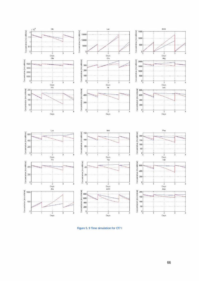
66

Figure 5. 9 Time simulation for CT7 I

67

Figure 5. 10 Time simulation for CT7 II

behaviour. One possible explanation could be that the cells after the first day begin to die; the cell growth for the sample CT7D3 is very low comparing with the other two. When the cells are dying the system works out of the bounds imposed for the pre-defined network and this will cause errors in the simulations as it can be seen in the graphs.

In the other hand it can be seen that some metabolites in the third sample fit as good as the sample CT7D1 that has been used to calculate the model, or even better, These are the cases of the Biomass, Ammonia, Glutamine, Arginine, Phenylanine, Threonine, Cysteine and Tyrosine. We could say that the model succeed in the prediction of the time evolution considering the such small errors that have been achieved when the model has been applied to data samples that has not been used to calculate it.

68

6. Conclusions, drawbacks and improvements In this here some final statements about the method and the results for the system object of study are done. In every part is discussed the validation, which are the drawbacks and how can it be improved.

6.1. Conclusions of the method The objective of the method is to find out an approximated dynamical model of a determined metabolic reaction network. If all the conditions specified in 3 (The method) are fulfilled, the obtained model will described quite accurately the system behaviour. However, the fulfilment of these conditions is not that easy to achieve.

From a beginning, the first condition is the most difficult to be fulfilled: the pre-defined network must be coherent with data used to calculate the model. The system must behave as it is defined in the metabolic network, what means that the metabolic pathways followed must be the ones in the network and must be followed in the directions described there. Otherwise, as the method is completely based on the pre-defined network, the model will lead to erroneous results. In order to avoid this, first the network should be properly defined. This can be done by metabolic flux analysis and make sure that the followed pathways are the ones supposed in the network.

Another drawback is the parameters or information needed to calculate the model. As explained in 3.2 (Design of the reduced dynamical model), the model requires sets of values of the state variable (consumption/production rates for a determined values of the metabolites concentrations). This values are not easy to obtain and depending on the method will be less or more accurate. The method that has been used to determine these sets of state variables is a linearization of the concentration along the time proposed by the KTH Division of Bioprocess. Of course, this is an estimation that will cause a different error depending on the nature of the system. In our case, by looking at the results obtained in the simulations, we could say that it is a good approximation. Nevertheless, it could be that some metabolites have faster exponential growth. In order to solve this, data in intermediate points of the process will be needed; not only of the initial and final point. In figure 6.1 and 6.2 a simulation of a model calculated only with one sample is shown. All the errors are around 1% or lower excepting the ones corresponding to Lactate (2.4%) and Ammonia, Asparagine and Aspartate (4.1%-4.9%). It can be seen that the graphs corresponding to Asparagine and Aspartate don’t have such a smooth growth as the other metabolites. But the error is not significant, considering that the error in the biological measurements is usually higher than these ones.

The other parameters needed are the half-saturation constants for every metabolite. For the network studied in this paper, the constants have been provided by the KTH Division of Bioprocess. The proper way to obtain these values would be to have previous studies of the concrete system. There are methods to estimate these constants [14] but some extra data is needed and consequently also resources. The proper selection of these constants will influence the quality of the model.

69

Figure 6. 1 Simulation of a model calculated with only one sample (CT7D1) I

70

Figure 6. 2 Simulation of a model calculated with only one sample (CT7D1) II

To assure a unique mathematical solution the condition specified in 3.2.2 (Fitting the maximal kinetic rate coefficients µj) ( · > ) must be fulfilled. This requires a determined number of samples that depends on the number of external metabolites and the complexity of the pre-defined metabolic network. Also has to be taken into account that the dynamical model only will assure the correct prediction of the behaviours that are represented for the data. For example, if Threonine, in the available samples is never produced, it is not assured that a model will be able to predict Threonine production under conditions where it should be. Also it could be that the model fails to describe the behaviour of the system if it is working in ranks of concentrations that are very far from the ones used to calculate the model. This is due to the fact that when the maximal kinetic rates are calculated the algorithm “chooses” the elementary flux modes that best fits with the data and it could be that some elementary modes correspond to pathways that would be used in other conditions. Then, if there’s no data that describes these conditions it can be that those pathways won’t be “chosen” for the final model. The conclusion is that the more data is available and the more conditions it describes a more reliable model will be obtained.

Another point is that when working with few samples is advisable to have more than one sample to describe the same conditions, otherwise a high error in the measurements in one sample can destabilize the values of the maximal kinetic rates inducing to big errors in the predictions. An example of this is the case of the Tyrosine in sample CT3D1 exposed in 5.6 (Final results).

If all this previous requirements are fulfilled and a reliable model is achieved, a tool that can predict the system evolution in any combination of conditions working in similar ranks to the data ones will be obtained. This can be used to select the proper initial concentrations if what

71

is wanted is to lead the system to a certain state or to minimize or maximize the production of determined metabolites, etc.

6.2. Conclusions of the results for the system object of study We can conclude that the obtained model succeed in the prediction of the system behaviour under initial conditions similar to the samples that have been used to calculate it as it is shown in 5.6 (Final results) and 5.7 (Time simulation). However we cannot assure that in other conditions the model will have a good response because we don’t have data to validate it. But what we can certainly know by looking at the implicit equations in the stoichiometric matrix in 5.6 (Final results) is the behaviours that the system described for the model will adopt under simulations. For example, if the concentration of an essential amino acid is decreased also the consumption rate will be decreased, or if there is less concentration of amino acids or glucose, the biomass growth will be also mitigated. A lot of predictions of this kind can be done, but as long as we don’t have data we cannot assure that they are correct.

Nevertheless the results can be improved. The main drawback is the lack of data that, as explained in the previous point, has two negative effects. First, the algorithm proposed in the method is not mathematically correct because the condition (3-29) in order to apply the least squares solving function is not fulfilled; even it hasn’t a very negative effect in the results. The other one is that some elementary flux modes that will participate in the final model aren’t used due to the fact that the data do not describe these situations. Just if the discarded data were coherent with the network the model would be more flexible when it comes to describe other situations.

Also the error caused for the concentration values of Asparagine and Serine that are considered as one is unknown. The model will improve if the separated values were available. Note that the condition · > would be fulfilled ( · = 6 · 24 = 144 > 143).

Of course as more experiments would be available more possibilities and a bigger rank of situations could be described by the model. The increase of experiments could be due to:

• Measurements in different levels of cell density, in order to see if the same equations useful or the system changes completely.

• Measurements in intermediate points of the growth, as explained above.

• Measurements in different levels of concentrations of the amino acids (not only removing the 100%, and including the essential amino acids also).

Apart of improving the available data, the network also could be modified to add more flexibility to the model. Some of the suggested modifications are:

• Add reactions representing the cell death and the dilution rates of the metabolites. This way the network could describe other phases, not only the growth phase.

• Try to remove from the initial network described in 2.3 (The available network) the co-metabolites that impede the fulfilment of the quasi steady-state conditions. The drawback in the actual model is that the biomass only can be described by a unique reaction and the influence in the cell growth of every metabolite is pre-defined by the stoichiometric matrix. If we could include the biomass production in the elementary

72

flux modes implying internal reactions, the weight of every metabolite in the final biomass production will be defined by the data as long as there would be several elementary flux modes that produce biomass. Unfortunately, this implies another drawback: the number of elementary flux modes will be increased and consequently more data will be needed.

6.3. Future works The good point is that when a new stoichiometric model is available or the model is wanted to be recalculated using new sets of data, the implemented tools described in 4 (Implementation) can calculate the new model just by changing the inputs. The first future work should be to find out a network than can describe all the possible conditions of interest and that described accurately the behaviours of the system. In order to achieve this not only can be done the improvements specified in this point but any other suggestions. The second future work would be to use the tool presented in this paper or an improved version in optimization problems of real engineering fields.

73

7. References [1] Biomed Central. A procedure for the estimation over time of metabolic fluxes in scenarios where measurements are uncertain and/or insufficient. Available at: <http://www.biomedcentral.com/1471-2105/8/421/figure/F4> [2009/08/09]. [2] E. Klipp, R. Herwing, A. Kowald, C. Wierling and H. Lehrach, Systems Biology in Practice, 5.2 Metabolic Networks (2005). [3] E. Klipp, R. Herwing, A. Kowald, C. Wierling and H. Lehrach, Systems Biology in Practice, 5.2.8 Metabolic Networks. Approximations on Timescale Separation (2005). [4] E. Klipp, R. Herwing, A. Kowald, C. Wierling and H. Lehrach, Systems Biology in Practice, 5.1.1 Metabolic Networks. The Law of Mass Action (2005). [5] C. Altamirano, A. Illanes, A. Casablancas, X. Gámez, J. Cairó and C. Godia, Analysis of CHO Cells Metabolic Redistribution in a Glutamate-Based Defined Medium in Continous Culture (2001). [6] A. Provost and G. Bastin, Metabolic Design of Macroscopic Models: Application to CHO cells (2005). [7] H. Bonarius and Co., Metabolic Flux Analysis of Hybrodoma Cells in Different Culture Using Mass Balances (1995). [8] A. Teixeira and Co., Hybrid elementary flux analysis/nonparametric modeling: application for bioprocess control (2007). [9] E. Klipp, R. Herwing, A. Kowald, C. Wierling and H. Lehrach, Systems Biology in Practice, 5.2.2 Metabolic Networks. Information Contained in the Stoichiometric Matrix N (2005). [10] Jena University. Bioinformatik. Metatool 5.1 for GNU octave and Matlab. Available at: <http://pinguin.biologie.uni-jena.de/bioinformatik/networks/metatool/metatool5.1/metatool 5.1.html> [2009/05/23]. [11] E. Klipp, R. Herwing, A. Kowald, C. Wierling and H. Lehrach, Systems Biology in Practice, 5.1.3 Metabolism. Michaelis-Menten Kinetics (2005). [12] Lawson, C.L. and R.J. Hanson, Solving Least-Squares Problems, Prentice-Hall, Chapter 23, p. 161 (1974). [13] The Mathworks. Optimization Toolbox. Function list: non-negative least squares. Available at:<http://www.mathworks.com/access/helpdesk/help/toolbox/optim/index.html?/access/helpdesk/help/toolbox/optim/ug/bqnk0r0.html&http://www.mathworks.com/products/optimization/?BB=1> [2009/06/15]. [14] E. Klipp, R. Herwing, A. Kowald, C. Wierling and H. Lehrach, Systems Biology in Practice, 5.1.3.2 Metabolism. Parameter Estimation and Linearization of the Michaelis Menten Equation (2005).

http://www.biomedcentral.com/1471-2105/8/421/figure/F4>

http://pinguin.biologie.uni-jena.de/bioinformatik/networks/metatool/metatool5.1/metatool

http://www.mathworks.com/access/helpdesk/help/toolbox/optim/index.html?/access/hel

http://www.mathworks.com/products/optimiza

74

Appendix I: The available network [5]

Network reactions

75

Metabolic network diagram

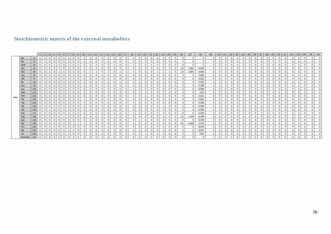
76

Stoichiometric matrix of the external metabolites

r1 r2 r3 r4 r5 r6 r7 r8 r9 r10 r11 r12 r13 r14 r15 r16 r17 r18 r19 r20 r21 r22 r23 r24 r25 r26 r27 r28 r29 r30 r31 r32 r33 r34 r35 r36 r37 r38 r39 r40 r41 r42 r43 r44 r45 r46

Aext

glc c1 -1 0 0 0 0 0 0 0 0 0 0 0 0 0 0 0 0 0 0 0 0 0 0 0 0 0 0 0 0 0 0 0 0 0 0 0 0 0 0 0 0 0 0 0 0 0

lac c2 0 1 0 0 0 0 0 0 0 0 0 0 0 0 0 0 0 0 0 0 0 0 0 0 0 0 0 0 0 0 0 0 0 0 0 0 0 0 0 0 0 0 0 0 0 0

NH4 c3 0 0 0 1 -1 0 1 0 -1 0 0 2 0 0 1 0 0 1 1 0 1 0 0 0 0 0 0 0 0 0 0 0 0 0 0 0 0 0 0 0 0 0 0 0 0 0

Gln c4 0 0 0 0 1 0 0 0 0 0 0 0 0 0 0 0 0 0 0 0 0 0 0 0 0 -1,9 -2,091 -0,052 0 0 0 0 0 0 0 0 0 0 0 0 0 0 0 0 0 0

Glu c5 0 0 -1 0 -1 -1 0 0 0 0 1 1 2 1 0 1 1 1 0 0 0 1 1 -1 0 1,9 2,091 -0,064 0 0 0 0 0 0 0 0 0 0 0 0 0 0 0 0 0 0

Arg c6 0 0 0 0 0 0 0 0 0 0 0 0 -1 0 0 0 0 0 0 0 0 0 0 0 0 0 0 -0,063 0 0 0 0 0 0 0 0 0 0 0 0 0 0 0 0 0 0

His c7 0 0 0 0 0 0 0 0 0 0 0 -1 0 0 0 0 0 0 0 0 0 0 0 0 0 0 0 -0,022 0 0 0 0 0 0 0 0 0 0 0 0 0 0 0 0 0 0

Ile c8 0 0 0 0 0 0 0 0 0 0 0 0 0 0 0 -1 0 0 0 0 0 0 0 0 0 0 0 -0,052 0 0 0 0 0 0 0 0 0 0 0 0 0 0 0 0 0 0

Leu c9 0 0 0 0 0 0 0 0 0 0 0 0 0 0 0 0 -1 0 0 0 0 0 0 0 0 0 0 -0,088 0 0 0 0 0 0 0 0 0 0 0 0 0 0 0 0 0 0

Lys c10 0 0 0 0 0 0 0 0 0 0 0 0 0 0 0 0 0 -1 0 0 0 0 0 0 0 0 0 -0,089 0 0 0 0 0 0 0 0 0 0 0 0 0 0 0 0 0 0

Met c11 0 0 0 0 0 0 0 0 0 0 0 0 0 0 0 0 0 0 -1 0 0 0 0 0 0 0 0 -0,02 0 0 0 0 0 0 0 0 0 0 0 0 0 0 0 0 0 0

Phe c12 0 0 0 0 0 0 0 0 0 0 0 0 0 0 0 0 0 0 0 -1 0 0 0 0 0 0 0 -0,021 0 0 0 0 0 0 0 0 0 0 0 0 0 0 0 0 0 0

Thr c13 0 0 0 0 0 0 0 0 0 -1 0 0 0 0 0 0 0 0 0 0 0 0 0 0 0 0 0 -0,061 0 0 0 0 0 0 0 0 0 0 0 0 0 0 0 0 0 0

Trp c14 0 0 0 0 0 0 0 0 0 0 0 0 0 0 0 0 0 0 0 0 -1 0 0 0 0 0 0 -0,006 0 0 0 0 0 0 0 0 0 0 0 0 0 0 0 0 0 0

Val c15 0 0 0 0 0 0 0 0 0 0 0 0 0 0 0 0 0 0 0 0 0 0 -1 0 0 0 0 -0,059 0 0 0 0 0 0 0 0 0 0 0 0 0 0 0 0 0 0

Ala c16 0 0 1 0 0 0 0 0 0 0 0 0 0 0 0 0 0 0 0 0 1 0 0 0 0 0 0 -0,095 0 0 0 0 0 0 0 0 0 0 0 0 0 0 0 0 0 0

Asn c17 0 0 0 0 0 0 0 0 0 0 0 0 0 0 -1 0 0 0 0 0 0 0 0 0 0 0 0 -0,039 0 0 0 0 0 0 0 0 0 0 0 0 0 0 0 0 0 0

Asp c18 0 0 0 0 0 1 0 0 0 0 0 0 0 0 1 0 0 0 0 0 0 0 0 0 0 -1,3 -1,194 -0,048 0 0 0 0 0 0 0 0 0 0 0 0 0 0 0 0 0 0

Cys c19 0 0 0 0 0 0 0 0 0 0 -1 0 0 0 0 0 0 0 1 0 0 0 0 0 0 0 0 -0,028 0 0 0 0 0 0 0 0 0 0 0 0 0 0 0 0 0 0

Gly c20 0 0 0 0 0 0 0 1 1 1 0 0 0 0 0 0 0 0 0 0 0 0 0 0 0 -0,5 -0,489 -0,078 0 0 0 0 0 0 0 0 0 0 0 0 0 0 0 0 0 0

Pro c21 0 0 0 0 0 0 0 0 0 0 0 0 0 -1 0 0 0 0 0 0 0 0 0 0 0 0 0 -0,028 0 0 0 0 0 0 0 0 0 0 0 0 0 0 0 0 0 0

Ser c22 0 0 0 0 0 0 -1 -1 0 0 0 0 0 0 0 0 0 0 -1 0 0 0 0 0 0 0 0 -0,057 0 0 0 0 0 0 0 0 0 0 0 0 0 0 0 0 0 0

Tyr c23 0 0 0 0 0 0 0 0 0 0 0 0 0 0 0 0 0 0 0 1 0 -1 0 0 0 0 0 -0,02 0 0 0 0 0 0 0 0 0 0 0 0 0 0 0 0 0 0

Biomass c24 0 0 0 0 0 0 0 0 0 0 0 0 0 0 0 0 0 0 0 0 0 0 0 0 0 0 0 0 1 0 0 0 0 0 0 0 0 0 0 0 0 0 0 0 0 0

77

Stoichiometric matrix of the internal metabolites

r1 r2 r3 r4 r5 r6 r7 r8 r9 r10 r11 r12 r13 r14 r15 r16 r17 r18 r19 r20 r21 r22 r23 r24 r25 r26 r27 r28 r29 r30 r31 r32 r33 r34 r35 r36 r37 r38 r39 r40 r41 r42 r43 r44 r45 r46

Aint

ATP c25 -1 0 0 0 -1 0 0 0 0 0 0 0 0 0 0 0 0 0 -3 0 0 0 0 0 0 -7,5 -7,487 -4 0 -1 2 0 0 0 0 0 0 0 0 0 0 -3,5 -17 0 3 2

ADP c26 1 0 0 0 1 0 0 0 0 0 0 0 0 0 0 0 0 0 3 0 0 0 0 0 0 7,5 7,487 4 0 1 -2 0 0 0 0 0 0 0 0 0 0 1 17 0 -3 -2

mATP c27 0 0 0 0 0 0 0 0 0 0 0 0 0 0 0 -1 -1 0 -1 0 0 0 -2 0 0 0 0 0 0 0 0 0 0 0 0 0 1 0 0 0 0 0 0 0 0 0

mADP c28 0 0 0 0 0 0 0 0 0 0 0 0 0 0 0 1 1 0 1 0 0 0 2 0 0 0 0 0 0 0 0 0 0 0 0 0 -1 0 0 0 0 0 0 0 0 0

NAD c29 0 1 0 0 0 0 0 0 1 0 0 0 -1 -2 0 0 0 0 -1 0 0 0 0 0 0 -0,7 -0,806 0 0 0 -1 0 0 0 0 0 0 0 0 1 0 0 9 0 1 0

NADH c30 0 -1 0 0 0 0 0 0 -1 0 0 0 1 2 0 0 0 0 1 0 0 0 0 0 0 0,7 0,806 0 0 0 1 0 0 0 0 0 0 0 0 -1 0 0 -9 0 -1 0

NADPH c31 0 0 0 0 0 0 0 0 0 0 0 -1 0 0 0 0 0 0 0 -1 -1 0 0 0 0 -0,3 0,978 0 0 0 0 2 0 0 0 0 0 0 0 0 1 0 -17 0 0 0

NADP c32 0 0 0 0 0 0 0 0 0 0 0 1 0 0 0 0 0 0 0 1 1 0 0 0 0 0,3 -0,978 0 0 0 0 -2 0 0 0 0 0 0 0 0 -1 0 7 0 0 0

mNAD c33 0 0 0 -1 0 0 0 0 0 -1 0 0 0 0 0 -2 -1 -2 -1 0 -3 0 -3 0 0 0,3 0,194 0 0 0 0 0 -1 0 -1 -1 0 0 -1 0 0 0 0 0 0 0

mNADH c34 0 0 0 1 0 0 0 0 0 1 0 0 0 0 0 2 1 2 1 0 3 0 3 0 0 -0,3 -0,194 0 0 0 0 0 1 0 1 1 0 0 1 0 0 0 0 0 0 0

FAD c35 0 0 0 0 0 0 0 0 0 0 0 0 0 0 0 0 0 0 0 0 0 0 0 0 0 0 0 0 0 0 0 0 0 0 0 0 0 0 0 0 0 0 0 0 0 1

FADH c36 0 0 0 0 0 0 0 0 0 0 0 0 0 0 0 0 0 0 0 0 0 0 0 0 0 0 0 0 0 0 0 0 0 0 0 0 0 0 0 0 0 0 0 0 0 -1

mFAD c37 0 0 0 0 0 0 0 0 0 0 0 0 0 0 0 -1 -1 -2 0 0 -1 0 -1 0 0 0 0 0 0 0 0 0 0 0 0 0 0 -1 0 0 0 0 0 0 0 0

mFADH c38 0 0 0 0 0 0 0 0 0 0 0 0 0 0 0 1 1 2 0 0 1 0 1 0 0 0 0 0 0 0 0 0 0 0 0 0 0 1 0 0 0 0 0 0 0 0

Pi c39 0 0 0 0 1 0 0 0 0 0 0 0 0 0 0 1 1 0 4 0 0 0 2 0 0 7,5 7,487 4 0 0 -1 0 0 0 0 0 -1 0 0 0 0 0 17 0 -3 -2

H2O c40 0 0 0 -1 0 0 0 1 0 0 0 -2 -2 -2 -1 -1 -1 -2 -4 1 -4 -2 -4 0 0 -3,1 -4,59 -4 0 0 1 -1 0 -1 0 0 0 -1 0 0 0 0 1 0 4 2

CO2 c41 0 0 0 0 0 0 0 0 -1 0 0 0 0 0 0 0 0 2 0 0 4 1 1 0 0 -0,5 -0,489 0 0 0 0 1 1 0 1 1 0 0 0 0 1 0 0 0 0 0

O2 c42 0 0 0 0 0 0 0 0 0 0 0 0 0 0 0 0 0 -0,5 0 -1 -3 -2 0 0 0 0 -0,097 0 0 0 0 0 0 0 0 0 0 0 0 0 0 0 -1 0 -0,5 -0,5

G6P c43 1 0 0 0 0 0 0 0 0 0 0 0 0 0 0 0 0 0 0 0 0 0 0 0 0 0 0 0 0 -1 0 -1 0 0 0 0 0 0 0 0 0 -1 0 0 0 0

Pyr c44 0 -1 -1 0 0 0 1 0 0 0 1 0 0 0 0 0 0 0 0 0 0 0 0 0 -1 0 0 0 0 0 1 0 0 0 0 0 0 0 0 0 1 0 0 0 0 0

alphaKG c45 0 0 1 0 0 1 0 0 0 0 -1 0 -1 0 0 -1 -1 -1 0 0 0 -1 -1 0 0 0 0 0 0 0 0 0 0 0 0 0 0 0 0 0 0 0 0 -1 0 0

Oxal c46 0 0 0 0 0 -1 0 0 0 0 0 0 0 0 0 0 0 0 0 0 0 0 0 0 0 0 0 0 0 0 0 0 0 0 0 0 0 0 0 -1 0 0 9 0 0 0

Mal c47 0 0 0 0 0 0 0 0 0 0 0 0 0 0 0 0 0 0 0 0 0 1 0 0 0 0,8 0,683 0 0 0 0 0 0 0 0 0 0 0 0 1 -1 0 -9 1 0 0

FH4 c48 0 0 0 0 0 0 0 -1 1 0 0 -1 0 0 0 0 0 0 -1 0 0 0 0 0 0 1,3 0,978 0 0 0 0 0 0 0 0 0 0 0 0 0 0 0 0 0 0 0

N5H10methylene c49 0 0 0 0 0 0 0 1 0 0 0 0 0 0 0 0 0 0 0 0 0 0 0 0 0 0 -0,978 0 0 0 0 0 0 0 0 0 0 0 0 0 0 0 0 0 0 0

N5H10methyleneFH4 c50 0 0 0 0 0 0 0 0 -1 0 0 1 0 0 0 0 0 0 1 0 0 0 0 0 0 -1,3 0 0 0 0 0 0 0 0 0 0 0 0 0 0 0 0 0 0 0 0

DHAP c51 0 0 0 0 0 0 0 0 0 0 0 0 0 0 0 0 0 0 0 0 0 0 0 0 0 0 0 0 0 2 -1 0 0 0 0 0 0 0 0 0 0 0 0 0 0 0

mPyr c52 0 0 0 0 0 0 0 0 0 0 0 0 0 0 0 0 0 0 0 0 0 0 0 0 1 0 0 0 0 0 0 0 -1 0 0 0 0 0 0 0 0 0 0 0 0 0

malphaKG c53 0 0 0 1 0 0 0 0 0 0 0 0 0 0 0 0 0 0 0 0 0 0 0 0 0 0 0 0 0 0 0 0 0 0 1 -1 0 0 0 0 0 0 0 1 0 0

mOxal c54 0 0 0 0 0 0 0 0 0 0 0 0 0 0 0 0 0 0 0 0 0 0 0 0 0 0 0 0 0 0 0 0 0 -1 0 0 0 0 1 0 0 0 0 0 0 0

mMal c55 0 0 0 0 0 0 0 0 0 0 0 0 0 0 0 0 0 0 0 0 0 0 0 0 0 0 0 0 0 0 0 0 0 0 0 0 0 1 -1 0 0 0 9 -1 0 0

mAcCoA c56 0 0 0 0 0 0 0 0 0 1 0 0 0 0 0 1 2 2 0 0 2 2 0 0 0 0 0 0 0 0 0 0 1 -1 0 0 0 0 0 0 0 0 0 0 0 0

mCoA c57 0 0 0 0 0 0 0 0 0 -1 0 0 0 0 0 -2 -1 -2 -1 0 -2 -1 -1 0 0 0 0 0 0 0 0 0 -1 1 0 -1 1 0 0 0 0 0 0 0 0 0

mSucCoA c58 0 0 0 0 0 0 0 0 0 0 0 0 0 0 0 1 -1 0 1 0 0 -1 1 0 0 0 0 0 0 0 0 0 0 0 0 1 -1 0 0 0 0 0 0 0 0 0

mSuc c59 0 0 0 0 0 0 0 0 0 0 0 0 0 0 0 0 1 0 0 0 0 0 0 0 0 0 0 0 0 0 0 0 0 0 0 0 1 -1 0 0 0 0 0 0 0 0

mGlu c60 0 0 0 -1 0 0 0 0 0 0 0 0 0 0 0 0 0 0 0 0 0 0 0 1 0 0 0 0 0 0 0 0 0 0 0 0 0 0 0 0 0 0 0 0 0 0

mCit c61 0 0 0 0 0 0 0 0 0 0 0 0 0 0 0 0 0 0 0 0 0 0 0 0 0 0 0 0 0 0 0 0 0 1 -1 0 0 0 0 0 0 0 -9 0 0 0

R5P c62 0 0 0 0 0 0 0 0 0 0 0 0 0 0 0 0 0 0 0 0 0 0 0 0 0 -1 -1 0 0 0 0 1 0 0 0 0 0 0 0 0 0 0 0 0 0 0

DNA c63 0 0 0 0 0 0 0 0 0 0 0 0 0 0 0 0 0 0 0 0 0 0 0 0 0 1 0 0 -0,135 0 0 0 0 0 0 0 0 0 0 0 0 0 0 0 0 0

RNA c64 0 0 0 0 0 0 0 0 0 0 0 0 0 0 0 0 0 0 0 0 0 0 0 0 0 0 1 0 -0,411 0 0 0 0 0 0 0 0 0 0 0 0 0 0 0 0 0

protein c65 0 0 0 0 0 0 0 0 0 0 0 0 0 0 0 0 0 0 0 0 0 0 0 0 0 0 0 1 -5,008 0 0 0 0 0 0 0 0 0 0 0 0 0 0 0 0 0

carbohydrates c66 0 0 0 0 0 0 0 0 0 0 0 0 0 0 0 0 0 0 0 0 0 0 0 0 0 0 0 0 -0,496 0 0 0 0 0 0 0 0 0 0 0 0 1 0 0 0 0

Oleic acid c67 0 0 0 0 0 0 0 0 0 0 0 0 0 0 0 0 0 0 0 0 0 0 0 0 0 0 0 0 -0,546 0 0 0 0 0 0 0 0 0 0 0 0 0 1 0 0 0

78

Appendix II: The new network

Network reactions R1. → 6 R13. ℎ → + R25. → 4 +

R2. 6 → 2 · 3 ℎ ℎ R14. → + 4 + R26. → 4 + 2

R3. 3 ℎ ℎ → R15. → 4 + R27. + ℎ →

R4. → R16. → + + R28. + 3 ℎ ℎ → +

R5. → + 2 R17. → 2 · + 2 · 2 R29. →

R6. + → R18. → + + 2 R30. ℎ →

R7. → + 2 R19. + → + 4 R31. → + 4

R8. → + 2 R20. → + 2 R32. → + 4

R9. → R21. + → Asp + R33. →

R10. → R22. → R34. →

R11. → R23. + → Ala + R35. → + 4

R12. → + 2 R24. → R36. + → +

R37. 0.0208 · + 0.0377 · + 0.0006 · + 0.007 · + 0.0033 · + 0.0084 · + 0.0133 · + 0.0101 · + 0.0033 · + 0.0055 · ℎ +0.008 · ℎ + 0.004 · + 0.0096 · + 0.0133 · + 0.026 · + 0.0004 · + 0.0165 · + 0.0081 · + 0.0099 · + 0.0077 · →

79

Network diagram

Pyr

AcCoA

Cit Oxal

αKG

Mal

SucCoA

Suc

CO2 Tyr

CO2

Leu

Val

Thr

Ser

Gly

CO2

Ile

NH4

Met

Cys

Lac

Glu

Asp

Asn

Gln

NH4

Ala

Ser

His

Arg

Pro

Trp

3-phosphoglycerate G6P Glc v1 v2 v3 v4

v6

v7

v8

v5

v9

v10

v11

v12

v13

v15 v16

v20

v19 v14

v17

v18

v21

v22

v23

v25 v26

v27

v28

v29

v34

v24

Phe v30

v31

v32

v33

v35

v37

v36

Lys

amino acids

BIOMASS

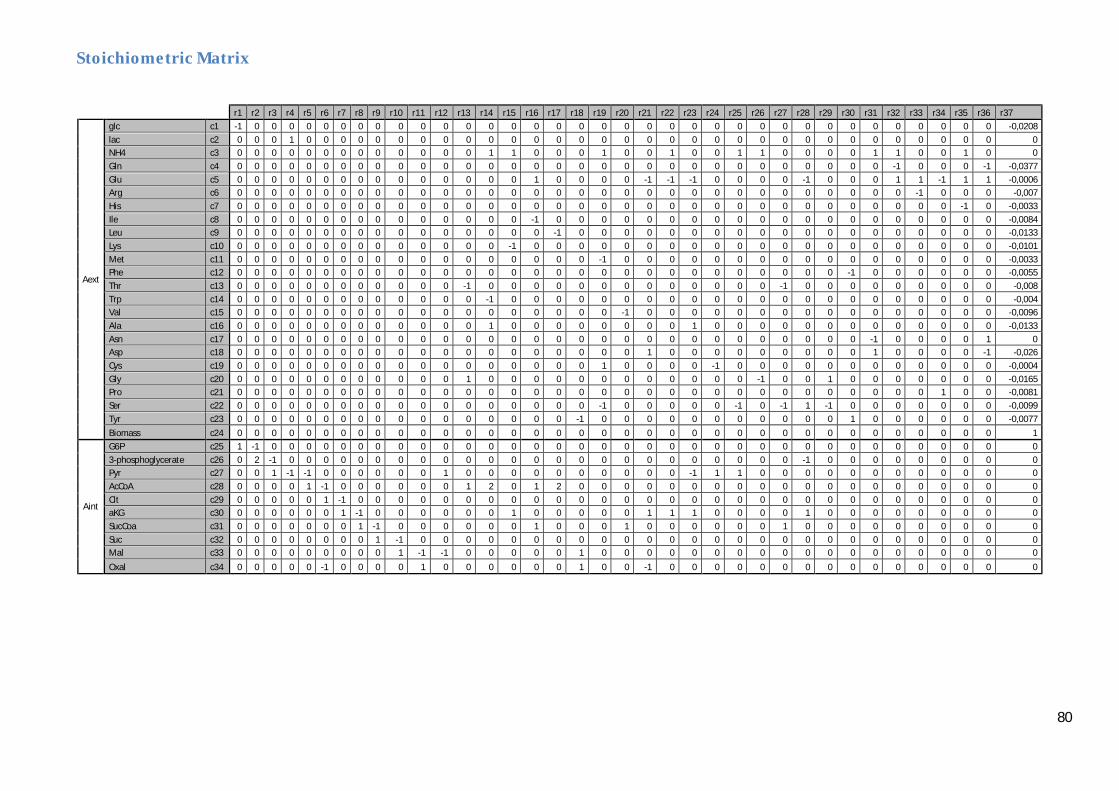
80

Stoichiometric Matrix

r1 r2 r3 r4 r5 r6 r7 r8 r9 r10 r11 r12 r13 r14 r15 r16 r17 r18 r19 r20 r21 r22 r23 r24 r25 r26 r27 r28 r29 r30 r31 r32 r33 r34 r35 r36 r37

Aext

glc c1 -1 0 0 0 0 0 0 0 0 0 0 0 0 0 0 0 0 0 0 0 0 0 0 0 0 0 0 0 0 0 0 0 0 0 0 0 -0,0208

lac c2 0 0 0 1 0 0 0 0 0 0 0 0 0 0 0 0 0 0 0 0 0 0 0 0 0 0 0 0 0 0 0 0 0 0 0 0 0 NH4 c3 0 0 0 0 0 0 0 0 0 0 0 0 0 1 1 0 0 0 1 0 0 1 0 0 1 1 0 0 0 0 1 1 0 0 1 0 0

Gln c4 0 0 0 0 0 0 0 0 0 0 0 0 0 0 0 0 0 0 0 0 0 0 0 0 0 0 0 0 0 0 0 -1 0 0 0 -1 -0,0377

Glu c5 0 0 0 0 0 0 0 0 0 0 0 0 0 0 0 1 0 0 0 0 -1 -1 -1 0 0 0 0 -1 0 0 0 1 1 -1 1 1 -0,0006 Arg c6 0 0 0 0 0 0 0 0 0 0 0 0 0 0 0 0 0 0 0 0 0 0 0 0 0 0 0 0 0 0 0 0 -1 0 0 0 -0,007

His c7 0 0 0 0 0 0 0 0 0 0 0 0 0 0 0 0 0 0 0 0 0 0 0 0 0 0 0 0 0 0 0 0 0 0 -1 0 -0,0033

Ile c8 0 0 0 0 0 0 0 0 0 0 0 0 0 0 0 -1 0 0 0 0 0 0 0 0 0 0 0 0 0 0 0 0 0 0 0 0 -0,0084 Leu c9 0 0 0 0 0 0 0 0 0 0 0 0 0 0 0 0 -1 0 0 0 0 0 0 0 0 0 0 0 0 0 0 0 0 0 0 0 -0,0133

Lys c10 0 0 0 0 0 0 0 0 0 0 0 0 0 0 -1 0 0 0 0 0 0 0 0 0 0 0 0 0 0 0 0 0 0 0 0 0 -0,0101

Met c11 0 0 0 0 0 0 0 0 0 0 0 0 0 0 0 0 0 0 -1 0 0 0 0 0 0 0 0 0 0 0 0 0 0 0 0 0 -0,0033 Phe c12 0 0 0 0 0 0 0 0 0 0 0 0 0 0 0 0 0 0 0 0 0 0 0 0 0 0 0 0 0 -1 0 0 0 0 0 0 -0,0055

Thr c13 0 0 0 0 0 0 0 0 0 0 0 0 -1 0 0 0 0 0 0 0 0 0 0 0 0 0 -1 0 0 0 0 0 0 0 0 0 -0,008

Trp c14 0 0 0 0 0 0 0 0 0 0 0 0 0 -1 0 0 0 0 0 0 0 0 0 0 0 0 0 0 0 0 0 0 0 0 0 0 -0,004 Val c15 0 0 0 0 0 0 0 0 0 0 0 0 0 0 0 0 0 0 0 -1 0 0 0 0 0 0 0 0 0 0 0 0 0 0 0 0 -0,0096

Ala c16 0 0 0 0 0 0 0 0 0 0 0 0 0 1 0 0 0 0 0 0 0 0 1 0 0 0 0 0 0 0 0 0 0 0 0 0 -0,0133

Asn c17 0 0 0 0 0 0 0 0 0 0 0 0 0 0 0 0 0 0 0 0 0 0 0 0 0 0 0 0 0 0 -1 0 0 0 0 1 0 Asp c18 0 0 0 0 0 0 0 0 0 0 0 0 0 0 0 0 0 0 0 0 1 0 0 0 0 0 0 0 0 0 1 0 0 0 0 -1 -0,026

Cys c19 0 0 0 0 0 0 0 0 0 0 0 0 0 0 0 0 0 0 1 0 0 0 0 -1 0 0 0 0 0 0 0 0 0 0 0 0 -0,0004

Gly c20 0 0 0 0 0 0 0 0 0 0 0 0 1 0 0 0 0 0 0 0 0 0 0 0 0 -1 0 0 1 0 0 0 0 0 0 0 -0,0165 Pro c21 0 0 0 0 0 0 0 0 0 0 0 0 0 0 0 0 0 0 0 0 0 0 0 0 0 0 0 0 0 0 0 0 0 1 0 0 -0,0081

Ser c22 0 0 0 0 0 0 0 0 0 0 0 0 0 0 0 0 0 0 -1 0 0 0 0 0 -1 0 -1 1 -1 0 0 0 0 0 0 0 -0,0099

Tyr c23 0 0 0 0 0 0 0 0 0 0 0 0 0 0 0 0 0 -1 0 0 0 0 0 0 0 0 0 0 0 1 0 0 0 0 0 0 -0,0077

Biomass c24 0 0 0 0 0 0 0 0 0 0 0 0 0 0 0 0 0 0 0 0 0 0 0 0 0 0 0 0 0 0 0 0 0 0 0 0 1

Aint

G6P c25 1 -1 0 0 0 0 0 0 0 0 0 0 0 0 0 0 0 0 0 0 0 0 0 0 0 0 0 0 0 0 0 0 0 0 0 0 0

3-phosphoglycerate c26 0 2 -1 0 0 0 0 0 0 0 0 0 0 0 0 0 0 0 0 0 0 0 0 0 0 0 0 -1 0 0 0 0 0 0 0 0 0 Pyr c27 0 0 1 -1 -1 0 0 0 0 0 0 1 0 0 0 0 0 0 0 0 0 0 -1 1 1 0 0 0 0 0 0 0 0 0 0 0 0

AcCoA c28 0 0 0 0 1 -1 0 0 0 0 0 0 1 2 0 1 2 0 0 0 0 0 0 0 0 0 0 0 0 0 0 0 0 0 0 0 0

Cit c29 0 0 0 0 0 1 -1 0 0 0 0 0 0 0 0 0 0 0 0 0 0 0 0 0 0 0 0 0 0 0 0 0 0 0 0 0 0 aKG c30 0 0 0 0 0 0 1 -1 0 0 0 0 0 0 1 0 0 0 0 0 1 1 1 0 0 0 0 1 0 0 0 0 0 0 0 0 0

SucCoa c31 0 0 0 0 0 0 0 1 -1 0 0 0 0 0 0 1 0 0 0 1 0 0 0 0 0 0 1 0 0 0 0 0 0 0 0 0 0

Suc c32 0 0 0 0 0 0 0 0 1 -1 0 0 0 0 0 0 0 0 0 0 0 0 0 0 0 0 0 0 0 0 0 0 0 0 0 0 0 Mal c33 0 0 0 0 0 0 0 0 0 1 -1 -1 0 0 0 0 0 1 0 0 0 0 0 0 0 0 0 0 0 0 0 0 0 0 0 0 0

Oxal c34 0 0 0 0 0 -1 0 0 0 0 1 0 0 0 0 0 0 1 0 0 -1 0 0 0 0 0 0 0 0 0 0 0 0 0 0 0 0

81

Appendix III: Calculations from data (ci and qi)

[Ala]0=0 [Asn]0=0 [Asp]0=0 [Cys]0=0 [Gln]0=0 [Glu]0=0

Day1 Day2 Day3 Day1 Day2 Day3 Day1 Day2 Day3 Day1 Day2 Day3 Day1 Day2 Day3 Day1 Day2 Day3

CT1 CT2 CT3 CT4 CT5 CT6

ci micromol/litre

c1 glc 16440,000 15560,000 16575,000 16130,000 15045,000 16305,000 16115,000 15440,000 16355,000 16315,000 18000,000 18410,000 - 17885,000 18215,000 15740,000 14770,000 15755,000

c2 lac 3475,000 5940,000 2205,000 2550,000 6365,000 1965,000 2985,000 5350,000 1770,000 2630,000 0,000 0,000 - 0,000 0,000 3705,000 7650,000 4715,000

c3 NH4 309,755 324,305 234,455 360,663 310,020 274,643 341,517 286,010 268,257 366,800 336,681 213,420 - 91,731 44,528 363,487 450,106 310,360

c4 Gln 3785,000 3860,000 3925,000 3810,000 3815,000 3880,000 3795,000 3860,000 3895,000 3835,000 4020,000 4025,000 - 0,000 0,000 3835,000 3840,000 3875,000

c5 Glu 287,055 309,029 291,394 304,098 326,960 289,331 283,799 287,824 314,371 299,122 303,897 277,331 - 290,688 293,912 67,520 111,945 78,666

c6 Arg 1771,974 1910,639 1770,022 1735,194 1908,332 1746,380 1755,667 2021,601 1695,947 1794,574 1920,345 1818,632 - 1933,107 1802,482 1694,097 1854,286 1683,342

c7 His 144,312 151,920 132,439 123,189 137,815 173,308 124,988 141,204 138,007 148,307 143,557 145,362 - 213,846 208,256 148,307 138,053 145,330

c8 Ile 419,158 449,187 443,373 413,346 443,405 447,475 422,118 462,903 432,225 427,294 448,427 453,596 - 441,559 470,914 408,034 433,281 426,232

c9 Leu 625,868 698,471 667,026 621,111 689,200 674,994 629,112 721,034 654,801 641,380 714,995 681,237 - 691,948 711,763 611,526 672,978 639,251

c10 Lys 514,037 597,795 556,805 505,588 583,778 576,913 529,611 584,173 559,729 529,216 609,136 553,932 - 604,620 612,139 498,183 562,143 559,724

c11 Met 119,487 127,957 124,385 115,854 127,365 122,933 119,204 135,196 119,358 122,018 137,190 129,194 - 131,895 129,748 114,052 121,756 116,236

c12 Phe 192,207 202,217 197,546 182,840 201,712 190,063 187,840 215,310 184,538 189,816 212,876 207,873 - 206,798 200,440 178,411 190,941 181,635

c13 Thr 422,449 412,252 435,830 421,334 410,774 432,727 420,050 459,456 420,706 434,058 442,735 446,172 - 445,147 449,901 411,061 427,779 405,870

c14 Trp 48,281 50,604 50,916 49,522 49,522 43,934 43,177 49,460 45,401 48,131 54,658 53,724 - 51,639 50,945 40,707 43,584 42,121

c15 Val 567,428 613,138 597,411 565,815 605,456 602,213 571,487 631,462 581,831 584,323 629,927 601,635 - 618,770 628,608 555,558 593,911 566,918

c16 Ala 161,415 100,176 49,202 365,572 324,654 254,458 345,741 298,544 276,384 390,969 311,116 151,245 - 248,182 236,266 344,044 303,766 258,102

c17 Asn+Ser 693,727 698,470 735,005 548,720 530,378 644,731 693,112 737,583 643,152 717,834 778,543 740,263 - 649,505 746,910 680,983 683,288 668,498

c18 Asp 158,735 157,624 169,239 179,300 161,720 100,785 19,072 13,426 97,134 175,190 183,416 158,877 - 166,417 190,134 158,358 148,665 152,472

c19 Cys 704,754 790,326 713,117 694,751 807,421 674,584 683,721 830,424 693,782 24,838 0,000 408,091 - 781,689 729,033 671,189 744,377 668,892

c20 Gly 323,880 378,662 321,436 312,996 368,684 299,786 305,534 377,239 299,765 307,103 323,367 327,028 - 412,736 311,793 299,585 360,346 296,073

c21 Pro 399,798 437,016 434,585 387,873 416,737 431,965 399,649 451,771 401,945 385,137 419,807 435,165 - 400,411 402,304 370,499 393,579 374,776

c22 Tyr 318,510 309,982 285,977 183,005 301,749 268,350 164,843 327,900 270,399 299,395 320,511 304,492 - 315,693 288,873 310,717 308,767 277,692

10^3cells c23 Biomass 530,000 534,000 466,000 567,000 684,500 492,600 549,500 517,000 466,100 548,000 400,000 270,000 - 385,500 249,900 560,000 610,000 577,600

qi nmol/10^6cells

q1 glc -4000 -7067,3953 -4174,1877 -4832,4515 -7173,1191 -4851,8067 -5040,9463 -7504,5537 -5166,9675 -4324,8175 1460,92038 3694,68128 - 1402,55009 3226,5343 -6285,7143 -7976,6253 -7084,8559

q2 lac 13113,2075 21639,3443 9950,36101 8994,70899 18597,5164 7978,07552 10864,4222 19489,9818 7987,36462 9598,54015 0 0 - 0 0 13232,1429 22352,0818 19143,3212

q3 NH4 1168,88709 1181,43816 1058,01192 1272,18046 905,828117 1115,07659 1243,00929 1041,92934 1210,54664 1338,68483 983,727564 866,506034 - 334,175123 200,936755 1298,16809 1315,13762 1260,08771

q4 Gln -811,32075 -510,01821 -338,44765 -670,194 -540,54054 -487,21072 -746,13285 -510,01821 -473,82671 -602,18978 58,4368152 101,502233 - 0 0 -589,28571 -467,49452 -507,51117

q5 Glu 109,444891 185,708274 150,461592 162,41809 201,337858 126,99363 93,7101466 108,457102 254,148641 149,891586 133,952967 78,2761955 - 118,891805 161,822403 241,141437 327,084931 319,392457

q6 Arg 25,0114799 529,303649 21,1021745 -106,35598 417,783239 -77,003573 -35,227524 933,537263 -313,17136 106,674813 452,883566 216,348837 - 611,153282 167,583349 -254,4584 259,870532 -332,94164

q7 His -91,826297 -60,931599 -163,38621 -160,34199 -90,082289 18,9310646 -158,90069 -99,968969 -138,26167 -74,229925 -73,305303 -94,533942 - 164,663522 178,745764 -72,639284 -89,387225 -94,664065

q8 Ile -136,98347 -22,848262 -54,539582 -148,54558 -35,217661 -32,413282 -121,34864 27,1180222 -104,84532 -102,79125 -20,545367 -7,563735 - -50,635811 69,7430594 -169,37363 -64,800402 -118,66416

q9 Leu -215,3658 56,5793173 -71,813456 -218,0931 18,2890707 -32,261816 -195,91855 138,77568 -126,98225 -151,68125 93,6579424 -6,9167498 - 32,8136778 130,068723 -255,05243 -29,108679 -177,38328

q10 Lys -108,5324 200,354393 63,2081459 -131,25124 119,73764 138,511647 -47,994808 150,730472 76,4052328 -49,569175 193,827959 45,2038494 - 225,217754 312,912276 -159,33948 56,5228714 68,7194674

q11 Met -30,375247 1,53210908 -14,220421 -41,207224 -0,5009503 -18,689665 -30,326482 27,9033641 -36,905334 -20,139048 28,2042778 6,72935094 - 15,8764087 9,97965999 -48,158134 -16,889518 -45,88053

q12 Phe -26,850627 10,5450323 -8,0175008 -58,140414 6,98101654 -37,594351 -41,794106 58,2407039 -66,717291 -34,694684 39,6001729 34,7142815 - 27,2349906 5,04230153 -74,683321 -24,489232 -71,812559

q13 Thr -68,871029 -103,63578 -21,978654 -68,312761 -87,439629 -32,373564 -75,160522 68,3285225 -90,227236 -24,24047 5,9464218 22,2170425 - 16,200431 41,5178242 -105,85345 -37,753805 -141,41432

q14 Trp 11,5431198 19,6044514 25,6952065 15,165839 12,5624992 -5,2319869 -7,4443828 15,437254 0,80581768 10,6145512 27,5697756 34,5159657 - 23,3775574 25,8236701 -16,127309 -4,7876078 -12,592424

q15 Val -151,79778 19,9764925 -46,227181 -147,58347 -6,4251339 -22,092262 -131,63864 86,7276367 -116,53162 -85,151156 65,0760717 -24,441984 - 40,491453 94,5532172 -186,0608 -40,158406 -165,39582

q16 Ala 609,1149 364,938459 222,028703 567,349965 350,402524 201,907499 513,239584 341,769784 323,3558 679,710023 310,846339 -217,14788 - 158,299313 142,31682 497,557005 289,373153 216,703468

q17 Asn+Ser -322,50283 -294,06208 -199,39342 -183,51173 -205,6045 178,583959 -313,29671 -151,57614 -613,89368 -223,92874 -1,8911998 -158,04906 - -472,44321 -145,66963 -350,74046 -280,21072 -449,42113

q18 Asp -57,978785 -60,019662 -21,931031 18,3440388 -36,171187 -297,66244 69,4144842 48,9114614 438,328474 3,98188921 27,2235674 -61,803033 - -27,986636 72,3617919 -56,217409 -74,31413 -87,806852

q19 Cys 40,5316851 350,868957 86,2076883 2,60298002 331,359502 -78,883525 -37,458679 496,942729 -1,0409045 90,6500913 0 1656,88466 - 319,403635 158,03488 -81,514755 147,156389 -101,99446

q20 Gly 270,910659 461,10476 312,936411 214,840548 340,671151 193,653796 194,524163 455,922058 215,146142 200,78324 208,263697 304,258885 - 585,234694 269,424879 169,628476 316,31104 178,578109

q21 Pro -10,858498 125,100738 143,993448 -52,21209 41,0858931 118,917371 -11,014932 178,854077 -3,2973379 -64,009432 50,0557374 131,911815 - -8,2493828 -1,6747616 -114,9175 -26,578026 -113,27298

q22 Tyr 12,6038345 -18,902078 -131,7384 -466,19067 -39,2152 -190,0935 -547,14337 46,3724742 -202,03782 -57,575906 15,6043562 -43,353882 - 1,90555956 -118,67028 -15,905974 -18,709435 -152,16391

10^3cells/10^6cells q23 Biomass 113,207547 69,2167577 -50,541516 236,33157 327,246165 -190,8242 180,163785 280,510018 -41,064982 175,182482 0 -203,00447 - -107,46812 -157,49097 214,285714 333,089847 -6,4961429

Essential amino acids

Incompatible with the network

82

[Gly]0=0 [Pro]0=0 [Ser]0=0 [Tyr]0=0 [Trp ]0=0 [C ]0= C0

Day1 Day2 Day3 Day1 Day2 Day3 Day1 Day2 Day3 Day1 Day2 Day3 Day1 Day2 Day3 Day1 Day2 Day3

CT7 CT8 CT9 CT10 CT11 CT12

ci micromol/litre

c1 glc 15760,000 15300,000 15745,000 - 17855,000 18505,000 15775,000 15350,000 16180,000 15935,000 15350,000 17955,000 16050,000 17050,000 18135,000 16110,000 14675,000 16170,000

c2 lac 3290,000 6560,000 4355,000 - 0,000 0,000 3575,000 5280,000 4915,000 3005,000 5280,000 0,000 2565,000 90,000 0,000 3575,000 6835,000 2240,000

c3 NH4 356,676 407,915 312,921 - 435,940 282,338 361,336 406,305 344,130 377,276 476,799 278,622 364,292 463,573 233,225 337,363 318,590 235,313

c4 Gln 3775,000 3865,000 3865,000 - 3970,000 4005,000 3790,000 3890,000 3890,000 3825,000 3890,000 3980,000 3835,000 3980,000 4045,000 3810,000 3930,000 3965,000

c5 Glu 286,309 322,091 304,679 - 339,747 298,135 292,985 322,796 302,726 301,044 383,687 310,059 305,901 392,639 300,860 277,178 304,558 286,627

c6 Arg 1659,993 1838,016 1705,675 - 1885,855 1750,407 1703,489 1900,893 1700,488 1706,622 1901,027 1747,022 1716,890 1881,740 1727,373 1720,287 1850,388 1689,447

c7 His 140,914 166,688 134,226 - 131,737 96,645 143,059 139,486 141,779 136,697 130,162 117,736 135,080 143,759 139,105 137,456 132,939 135,132

c8 Ile 399,042 430,440 435,257 - 444,927 460,977 407,597 439,074 433,582 407,488 443,510 455,382 411,610 442,493 456,543 410,190 437,307 438,669

c9 Leu 597,161 669,833 654,331 - 700,987 696,909 610,261 684,609 655,388 611,652 700,792 687,566 616,639 697,606 687,428 612,655 680,811 662,312

c10 Lys 486,498 556,095 581,702 - 593,780 591,553 498,895 566,030 562,269 501,707 595,795 590,407 520,535 599,213 573,578 495,956 573,286 562,534

c11 Met 111,412 121,251 119,311 - 133,633 127,238 114,522 126,512 118,903 115,143 133,959 127,120 117,433 132,740 125,719 116,761 125,174 120,572

c12 Phe 174,310 190,107 186,552 - 210,082 195,736 179,612 199,498 184,221 180,012 208,896 196,431 184,417 208,517 195,923 188,044 196,639 186,007

c13 Thr 402,219 421,904 416,886 - 433,597 438,562 412,182 440,986 420,166 413,878 436,925 435,793 414,986 438,295 435,309 413,201 425,927 415,664

c14 Trp 41,919 46,429 46,253 - 48,753 45,893 41,514 46,967 43,378 41,304 48,203 45,818 0,000 0,000 0,000 42,798 43,746 41,952

c15 Val 543,547 590,979 579,300 - 618,492 614,555 556,570 604,892 581,318 556,941 621,155 609,913 561,030 616,522 605,119 554,743 598,692 586,207

c16 Ala 342,550 304,883 276,973 - 288,086 227,648 351,349 302,326 273,026 354,051 304,044 227,991 363,944 313,663 239,834 345,321 306,696 259,464

c17 Asn+Ser 655,688 674,456 670,877 - 775,771 782,948 175,652 180,331 173,647 674,729 755,348 767,028 683,588 789,407 779,728 670,746 689,869 711,689

c18 Asp 166,496 169,761 173,627 - 182,488 190,272 162,867 163,461 168,397 169,863 187,018 192,150 171,384 175,346 180,935 157,922 154,329 169,987

c19 Cys 634,656 732,599 682,750 - 728,909 683,437 646,935 756,152 653,488 642,012 715,645 679,850 672,198 720,283 689,749 670,093 755,486 666,854

c20 Gly 88,867 126,971 85,678 - 343,658 263,021 265,771 260,067 245,002 315,796 393,230 279,106 320,952 340,035 245,486 312,572 375,453 296,069

c21 Pro 366,717 396,887 391,138 - 0,000 0,000 377,806 408,693 396,583 374,405 424,395 413,320 383,249 422,158 416,009 367,956 390,312 390,738

c22 Tyr 299,703 299,089 277,590 - 311,504 279,133 307,118 313,547 274,525 28,221 0,000 0,000 317,031 322,222 289,044 316,796 305,107 273,958

10^3cells c23 Biomass 607,000 570,000 579,500 - 456,000 295,500 584,500 576,000 504,700 582,500 597,500 390,700 578,500 403,000 180,400 527,000 554,500 431,700

qi nmol/10^6cells

q1 glc -5733,1137 -8014,5719 -7919,6751 - 1037,25347 4080,38977 -5902,4808 -7832,4226 -5956,6787 -5373,3906 -6281,9576 1847,34064 -5012,9646 -1639,3443 2865,52347 -5275,1423 -8254,2001 -5399,9188

q2 lac 10840,1977 23897,9964 19652,5271 - 0 0 12232,6775 19234,9727 22179,6029 10317,5966 15427,3192 0 8867,76145 327,868852 0 13567,3624 19970,7816 9094,60008

q3 NH4 1175,21041 1486,02871 1412,09763 - 1273,7467 1146,31557 1236,39376 1480,16503 1552,93441 1295,36744 1393,13101 1131,22827 1259,43702 1688,78876 1052,45763 1280,31432 930,86991 955,391385

q4 Gln -741,35091 -491,80328 -609,20578 - -87,655223 20,3004466 -718,56287 -400,7286 -496,38989 -600,85837 -321,40248 -81,201786 -570,4408 -72,859745 203,068592 -721,06262 -204,52885 -142,10313

q5 Glu 93,1031817 233,294362 210,409502 - 238,700711 162,74213 119,532247 235,859961 201,597787 147,613361 367,086134 211,152993 165,422939 490,297239 193,17638 72,5847756 135,883521 116,017875

q6 Arg -347,12408 264,739362 -269,26971 - 352,109215 -60,652691 -211,65615 493,798578 -292,67615 -201,62646 396,440624 -74,397149 -167,51988 424,024394 -171,35572 -170,99878 248,480844 -308,15469

q7 His -91,371934 -7,1299277 -155,32221 - -107,84171 -292,3272 -87,551286 -106,2282 -121,23953 -109,69408 -112,44208 -206,69843 -116,04486 -90,661321 -133,30654 -118,36782 -104,3296 -136,06874

q8 Ile -185,88724 -91,143601 -91,161048 - -30,772335 22,4066734 -163,77086 -59,689668 -98,723254 -164,70742 -34,911015 -0,3117517 -151,59535 -47,235156 4,89339517 -171,79679 -53,036316 -68,167185

q9 Leu -282,63313 -47,749703 -129,10249 - 52,7290637 56,7135089 -248,68851 6,07806505 -124,33454 -244,76523 52,1602569 18,7797605 -229,21719 53,4259979 20,2521844 -266,73872 -6,2209054 -83,753581

q10 Lys -185,50077 48,4408665 175,558114 - 148,960845 197,949453 -150,22492 84,6355908 87,8636258 -141,08581 154,848202 193,296069 -76,968465 205,518203 138,899845 -177,76811 89,0818453 80,1293159

q11 Met -53,129325 -22,898287 -37,117548 - 17,8118856 -1,212041 -44,531343 -3,7313184 -38,959789 -42,554601 18,7651637 -1,6902432 -34,931084 18,9566038 -8,200222 -40,893869 -6,9021542 -28,276667

q12 Phe -82,414634 -33,572764 -57,627412 - 31,4382225 -14,561269 -67,442395 0,63908184 -68,146278 -66,302091 27,9716197 -11,738499 -51,532631 33,4940723 -15,341148 -42,800679 -7,8414506 -54,060973

q13 Thr -126,79283 -68,475234 -107,46708 - -20,754275 -8,6816596 -97,582066 1,03957095 -92,664515 -92,09423 -11,030799 -19,925395 -88,898097 -8,7637451 -24,327595 -104,36261 -43,165669 -101,65077

q14 Trp -10,885743 4,39572758 4,64948199 - 10,3173105 2,72249705 -12,689209 6,35487969 -8,3218094 -13,453588 8,70773644 2,4193 0 0 0 -9,1989576 -4,3123801 -13,278019

q15 Val -211,2277 -60,751483 -127,9539 - 31,6639129 28,0138112 -174,79974 -10,065039 -118,8499 -174,12305 39,4441286 9,16683961 -161,19274 32,3023317 -11,441736 -200,80493 -26,18807 -87,081559

q16 Ala 454,107848 364,861578 326,013807 - 243,558057 93,0535079 501,696008 355,54637 308,200571 512,694406 290,184912 94,44882 550,444165 396,848925 158,420759 533,556906 297,933926 222,229425

q17 Asn+Ser -406,92642 -381,54493 -488,77983 - -9,9919517 15,254487 -9,5553494 6,87260111 -21,650885 -358,66692 -69,664388 -49,379609 -330,5182 37,2193725 2,42756585 -411,55235 -260,98244 -274,06334

q18 Asp -25,052461 -15,803569 -2,1302362 - 24,510695 65,6649282 -38,432451 -38,753565 -25,733582 -14,544478 37,7483859 73,2861775 -9,3871012 4,54317499 30,846588 -61,394488 -57,764705 -16,694073

q19 Cys -195,57348 140,56722 -50,825845 - 101,959388 -42,938615 -161,08887 226,370411 -182,87286 -178,54292 63,2066142 -57,501432 -75,418086 95,7014516 -19,239369 -90,776175 179,615003 -110,26648

q20 Gly 292,807905 462,555102 386,635453 - 267,552009 44,3842756 46,8173358 29,0634886 -31,978724 218,735888 412,391915 109,690775 238,076001 320,387874 -29,795308 229,5376 360,451873 178,563399

q21 Pro -118,48027 -21,088905 -52,065573 - 0 0 -85,098512 21,923073 -27,495492 -97,065947 63,4604725 43,2160038 -67,163046 70,9747511 60,1697411 -131,76415 -36,124068 -48,467179

q22 Tyr -50,961946 -58,583417 -169,58839 - -10,712712 -146,31434 -27,553145 -5,9147972 -183,41792 96,8964068 0 0 6,43076306 25,6883042 -117,89876 6,16753229 -29,402636 -167,32741

10^3cells/10^6cells q23 Biomass 352,553542 236,794171 322,65343 - 40,9057706 -326,83719 289,136014 134,790528 64,5306859 283,261803 45,2885318 -404,79091 271,39153 -262,29508 -380,86643 102,466793 39,4448503 -92,164028

Essential amino acids

Incompatible with the network

83

Appendix IV: Elementary Flux Modes and all their corresponding macroscopic reactions Amac

Elementary Flux Modes for the new network (e1-e50)

e1 e2 e3 e4 e5 e6 e7 e8 e9 e10 e11 e12 e13 e14 e15 e16 e17 e18 e19 e20 e21 e22 e23 e24 e25 e26 e27 e28 e29 e30 e31 e32 e33 e34 e35 e36 e37 e38 e39 e40 e41 e42 e43 e44 e45 e46 e47 e48 e49 e50

r1 0 0 0 0 0 0 0 0 0 0 0 0 1 0 0 0 0 0 0 0 0 0 0 0 0,5 0 0 0 0 0 0 0 0 0 0 0 0 0 0 0 0,5 0 0 0 0 0 0 0 0 0

r2 0 0 0 0 0 0 0 0 0 0 0 0 1 0 0 0 0 0 0 0 0 0 0 0 0,5 0 0 0 0 0 0 0 0 0 0 0 0 0 0 0 0,5 0 0 0 0 0 0 0 0 0

r3 0 0 0 0 0 0 0 0 0 0 0 0 2 0 0 0 0 0 0 0 0 0 0 0 0 0 0 0 0 0 0 0 0 0 0 0 0 0 0 0 0 0 0 0 0 0 0 0 0 0

r4 -1 -1 -1 -1 -1 1 1 1 1 2 1 1 2 1 1 1 1 1 1 2 1 2 1 2 1 1 3 1 1 1 1 1 1 1 1 1 2 2 3 2 1 1 1 2 1 1 2 -1 0 0

r5 1 1 1 1 1 0 0 0 0 0 0 0 0 0 0 0 0 0 0 0 0 0 0 0 0 0 0 0 0 0 0 0 0 1 0 0 0 0 0 0 0 1 0 0 0 0 0 0 0 0

r6 1 1 1 1 1 0 1 1 1 1 0 1 0 0 0 0 0 0 1 1 1 1 1 1 0 1 1 1 1 1 1 1 1 1 0 1 1 1 1 1 0 1 0 0 0 0 0 0 0 0

r7 1 1 1 1 1 0 1 1 1 1 0 1 0 0 0 0 0 0 1 1 1 1 1 1 0 1 1 1 1 1 1 1 1 1 0 1 1 1 1 1 0 1 0 0 0 0 0 0 0 0

r8 0 0 0 0 1 0 0 0 0 0 1 0 0 0 0 0 0 0 0 0 0 0 0 0 0 0 0 0 0 0 0 0 0 0 1 1 1 1 1 1 1 1 0 0 0 0 1 0 0 0

r9 0 1 1 0 1 0 0 0 0 1 1 1 0 0 0 1 1 0 0 0 0 0 0 0 0 1 1 1 1 1 1 1 1 0 1 2 1 1 2 1 1 1 0 0 1 1 1 0 0 1

r10 0 1 1 0 1 0 0 0 0 1 1 1 0 0 0 1 1 0 0 0 0 0 0 0 0 1 1 1 1 1 1 1 1 0 1 2 1 1 2 1 1 1 0 0 1 1 1 0 0 1

r11 0,5 1 1 0 1 0 0 0 0 0 0 0 0 0 0 0 0 0 0,5 0 0,5 0 0,5 0 0 1 0 1 1 1 1 1 1 0 0 1 0 0 0 0 0 0 0,5 0 1 1 0 0 1 1

r12 0 0 0 0 0 1 1 1 1 2 1 1 0 0 0 1 1 0 0 1 0 1 0 1 0 0 2 0 0 0 0 0 0 1 1 1 2 2 3 2 1 2 0 1 0 0 2 0 0 0

r13 0 0 0 0 0 0 1 0 0 0 0 0 0 0 0 0 0 0 1 1 0 0 0 0 0 0 0 1 0 0 1 0 0 0 0 0 1 0 0 0 0 0 0 0 0 0 0 0 0 0

r14 0 0 0 0 0 0 0 0,5 0 0 0 0 0 0 0 0 0 0 0 0 0,5 0,5 0 0 0 0 0 0 0,5 0 0 0,5 0 0 0 0 0 0,5 0 0 0 0 0 0 0 0 0 0 0 0

r15 0 0 0 0 0 0 0 0 0 0 0 0 0 0 0 0 0 1 0 0 0 0 0 0 0 0 0 0 0 0 0 0 0 0 1 0 0 0 0 0 0 0 0 0 0 0 0 0 0 0

r16 0 0 0 0 0 0 0 0 0 1 0 1 0 0 0 0 0 0 0 0 0 0 0 0 0 1 1 0 0 0 0 0 0 0 0 1 0 0 1 0 0 0 0 0 0 0 0 0 0 0

r17 0 0 0 0 0 0 0 0 0,5 0 0 0 0 0 0 0 0 0 0 0 0 0 0,5 0,5 0 0 0 0 0 0,5 0 0 0,5 0 0 0 0 0 0 0,5 0 0 0 0 0 0 0 0 0 0

r18 0,5 0 0 0 0 1 1 1 1 1 0 0 0 0 0 0 0 0 0,5 1 0,5 1 0,5 1 0 0 1 0 0 0 0 0 0 1 0 0 1 1 1 1 0 1 0,5 1 0 0 1 0 1 0

r19 0 0 0 0 0 0 0 0 0 0 0 0 0 0 0 0 0 0 0 0 0 0 0 0 0 0 0 0 0 0 0 0 0 0 0 0 0 0 0 0 0 0 0 0 0 0 0 0 0 0

r20 0 1 0 0 0 0 0 0 0 0 0 0 0 0 0 1 0 0 0 0 0 0 0 0 0 0 0 1 1 1 0 0 0 0 0 0 0 0 0 0 0 0 0 0 1 0 0 0 0 1

r21 0 0 0 -1 0 1 0 0 0 0 0 -1 0 0 0 0 0 0 0 0 0 0 0 0 0 0 0 0 0 0 0 0 0 0 0 0 0 0 0 0 0 0 1 1 1 1 1 0 2 1

r22 -1 -1 -1 0 0 -1 -1 -1 -1 -1 1 0 0 0 0 0 0 0 0 0 0 0 0 0 0 0 0 0 0 0 0 0 0 0 0 0 0 0 0 0 0 0 0 0 0 0 0 -1 -2 -1

r23 0 0 0 0 0 0 0 0 0 0 0 0 0 0 0 0 0 -1 -1 -1 -1 -1 -1 -1 -1 -1 -1 -1 -1 -1 -1 -1 -1 -1 0 0 0 0 0 0 0 0 -1 -1 -1 -1 0 1 0 0

r24 0 0 0 0 0 0 0 0 0 0 0 0 0 0 1 0 0 0 0 0 0 0 0 0 0 0 0 0 0 0 0 0 0 0 0 0 0 0 0 0 0 0 0 0 0 0 0 0 0 0

r25 0 0 0 0 0 0 0 0 0 0 0 0 0 1 0 0 0 0 0 0 0 0 0 0 0 0 0 0 0 0 0 0 0 0 0 0 0 0 0 0 0 0 0 0 0 0 0 0 0 0

r26 0 0 0 0 0 0 0 0 0 0 0 0 0 0 0 0 0 0 0 0 0 0 0 0 0 0 0 0 0 0 0 0 0 0 0 0 0 0 0 0 0 0 0 0 0 0 0 0 0 0

r27 0 0 1 0 0 0 0 0 0 0 0 0 0 0 0 0 1 0 0 0 0 0 0 0 0 0 0 0 0 0 1 1 1 0 0 0 0 0 0 0 0 0 0 0 0 1 0 0 0 0

r28 0 0 0 0 0 0 0 0 0 0 0 0 0 0 0 0 0 0 0 0 0 0 0 0 1 0 0 0 0 0 0 0 0 0 0 0 0 0 0 0 1 0 0 0 0 0 0 0 0 0

r29 0 0 0 0 0 0 0 0 0 0 0 0 0 0 0 0 0 0 0 0 0 0 0 0 0 0 0 0 0 0 0 0 0 0 0 0 0 0 0 0 0 0 0 0 0 0 0 0 0 0

r30 0 0 0 0 0 0 0 0 0 0 0 0 0 0 0 0 0 0 0 0 0 0 0 0 0 0 0 0 0 0 0 0 0 0 0 0 0 0 0 0 0 0 0 0 0 0 0 0 0 0

r31 0 0 0 0 0 0 0 0 0 0 0 0 0 0 0 0 0 0 0 0 0 0 0 0 0 0 0 0 0 0 0 0 0 0 0 0 0 0 0 0 0 0 0 0 0 0 0 0 0 0

r32 0 0 0 0 0 0 0 0 0 0 0 0 0 0 0 0 0 0 0 0 0 0 0 0 0 0 0 0 0 0 0 0 0 0 0 0 0 0 0 0 0 0 0 0 0 0 0 0 0 0

r33 0 0 0 0 0 0 0 0 0 0 0 0 0 0 0 0 0 0 0 0 0 0 0 0 0 0 0 0 0 0 0 0 0 0 0 0 0 0 0 0 0 0 0 0 0 0 0 0 0 0

r34 0 0 0 0 0 0 0 0 0 0 0 0 0 0 0 0 0 0 0 0 0 0 0 0 0 0 0 0 0 0 0 0 0 0 0 0 0 0 0 0 0 0 0 0 0 0 0 0 0 0

r35 0 0 0 0 0 0 0 0 0 0 0 0 0 0 0 0 0 0 0 0 0 0 0 0 0 0 0 0 0 0 0 0 0 0 0 0 0 0 0 0 0 0 0 0 0 0 0 0 0 0

r36 0 0 0 0 0 0 0 0 0 0 0 0 0 0 0 0 0 0 0 0 0 0 0 0 0 0 0 0 0 0 0 0 0 0 0 0 0 0 0 0 0 0 0 0 0 0 0 0 0 0

r37 0 0 0 0 0 0 0 0 0 0 0 0 0 0 0 0 0 0 0 0 0 0 0 0 0 0 0 0 0 0 0 0 0 0 0 0 0 0 0 0 0 0 0 0 0 0 0 0 0 0

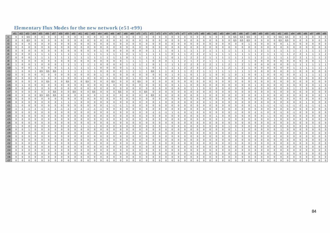
84


e51 e52 e53 e54 e55 e56 e57 e58 e59 e60 e61 e62 e63 e64 e65 e66 e67 e68 e69 e70 e71 e72 e73 e74 e75 e76 e77 e78 e79 e80 e81 e82 e83 e84 e85 e86 e87 e88 e89 e90 e91 e92 e93 e94 e95 e96 e97 e98 e99

r1 0 0 0,5 0 0 0 0 0 0 0 0 0 0 0 0 0 0 0 0 0 0 0 0 0 0 0 0 0 0 0 0 0 0 0 0,5 0,5 0,5 0 0 0 0 0,5 0,5 0 0 0 0 0 0

r2 0 0 0,5 0 0 0 0 0 0 0 0 0 0 0 0 0 0 0 0 0 0 0 0 0 0 0 0 0 0 0 0 0 0 0 0,5 0,5 0,5 0 0 0 0 0,5 0,5 0 0 0 0 0 0

r3 0 0 0 0 0 0 0 0 0 0 0 0 0 0 0 0 0 0 0 0 0 0 0 0 0 0 0 0 0 0 0 0 0 0 0 0 1 0 0 0 0 0 1 0 0 0 0 0 0

r4 0 0 0 0 0 0 0 0 0 0 0 0 0 0 0 0 0 0 0 0 0 0 0 0 0 0 0 0 0 0 0 0 0 0 0 0 0 0 0 0 0 0 0 0 0 0 0 0 0

r5 0 0 0 0 0 0 0 0 0 0 0 0 0 1 0 0 0 0 0 0 0 1 1 1 0 1 1 1 1 2 1 1 1 1 1 1 1 1 2 1 1 1 1 1 1 1 1 1 2

r6 0 0 0 1 1 1 1 1 1 1 1 1 1 1 1 1 1 0 1 1 1 1 1 1 0 1 1 2 2 2 1 1 1 1 1 1 1 1 2 1 1 1 1 2 2 1 1 1 2

r7 0 0 0 1 1 1 1 1 1 1 1 1 1 1 1 1 1 0 1 1 1 1 1 1 0 1 1 2 2 2 1 1 1 1 1 1 1 1 2 1 1 1 1 2 2 1 1 1 2

r8 0 0 0 0 0 0 0 0 0 0 0 0 0 0 0 0 0 1 1 1 1 0 0 0 1 1 2 1 2 2 1 1 1 1 1 2 1 0 0 0 0 0 0 0 0 0 0 1 1

r9 1 0 0 1 0 0 0 1 1 1 1 1 1 0 0 0 0 1 1 1 1 0 1 1 1 1 2 2 3 2 2 1 1 2 1 2 1 0 0 0 0 0 0 1 1 1 1 1 1

r10 1 0 0 1 0 0 0 1 1 1 1 1 1 0 0 0 0 1 1 1 1 0 1 1 1 1 2 2 3 2 2 1 1 2 1 2 1 0 0 0 0 0 0 1 1 1 1 1 1

r11 1 0 0 1 0,5 0,5 0,5 1 1 1 1 1 1 0 0 0 0 1 1 1 1 0,5 1 1 0 1 1 2 2 1 1 1 1 1 1 1 1 0 0 0 0 0 0 1 0 0 0 0 0

r12 0 0 0 0 0 0 0 0 0 0 0 0 0 1 0 0 0 0 0 0 0 0 0 0 1 0 1 0 1 2 1 0 0 1 0 1 0 0 1 0 0 0 0 0 1 1 1 1 2

r13 0 0 0 0 1 0 0 1 0 0 1 0 0 0 1 0 0 0 1 0 0 0 0 0 0 0 0 0 0 0 0 0 0 0 0 0 0 0 0 0 0 0 0 0 0 0 0 0 0

r14 0 0 0 0 0 0,5 0 0 0,5 0 0 0,5 0 0 0 0,5 0 0 0 0,5 0 0 0 0 0 0 0 0 0 0 0 0 0 0 0 0 0 0 0 0 0 0 0 0 0 0 0 0 0

r15 0 1 0 0 0 0 0 0 0 0 0 0 0 0 0 0 0 0 0 0 0 0 0 0 0 1 1 0 0 0 0 0 0 0 0 0 0 1 0 0 0 0 0 0 0 0 0 1 0

r16 0 0 0 1 0 0 0 0 0 0 0 0 0 0 0 0 0 0 0 0 0 0 0 0 0 0 0 1 1 0 0 0 0 0 0 0 0 0 0 0 0 0 0 1 1 0 0 0 0

r17 0 0 0 0 0 0 0,5 0 0 0,5 0 0 0,5 0 0 0 0,5 0 0 0 0,5 0 0 0 0 0 0 0 0 0 0 0 0 0 0 0 0 0 0 0 0 0 0 0 0 0 0 0 0

r18 0 0 0 0 0,5 0,5 0,5 0 0 0 0 0 0 1 0 0 0 0 0 0 0 0,5 0 0 0 0 0 0 0 1 0 0 0 0 0 0 0 0 1 0 0 0 0 0 0 0 0 0 1

r19 0 0 0 0 0 0 0 0 0 0 0 0 0 0 0 0 0 0 0 0 0 0 0 0 0 0 0 0 0 0 0 0 0 0 0 0 0 0 0 0 0 0 0 0 0 0 0 0 0

r20 0 0 0 0 0 0 0 1 1 1 0 0 0 0 0 0 0 0 0 0 0 0 1 0 0 0 0 0 0 0 1 0 0 0 0 0 0 0 0 0 0 0 0 0 0 1 0 0 0

r21 1 0 0 0 0 0 0 0 0 0 0 0 0 0 -1 -1 -1 1 0 0 0 0 0 0 0 0 0 0 0 0 0 0 0 0 0 0 0 -1 -1 -1 -1 -1 -1 -1 -2 -1 -1 -1 -1

r22 -1 -1 -1 -1 -1 -1 -1 -1 -1 -1 -1 -1 -1 -1 0 0 0 0 0 0 0 0 0 0 0 0 0 0 0 0 0 0 0 0 0 0 0 0 0 0 0 0 0 0 0 0 0 0 0

r23 0 0 0 0 0 0 0 0 0 0 0 0 0 0 0 0 0 0 0 0 0 -1 -1 -1 1 -1 0 -1 0 0 0 0 0 0 -1 0 0 -1 -1 0 0 -1 0 -1 0 0 0 0 0

r24 0 0 0 0 0 0 0 0 0 0 0 0 0 0 0 0 0 0 0 0 0 0 0 0 0 0 0 0 0 0 0 1 0 0 0 0 0 0 0 1 0 0 0 0 0 0 0 0 0

r25 0 0 0 0 0 0 0 0 0 0 0 0 0 0 0 0 0 0 0 0 0 0 0 0 0 0 0 0 0 0 0 0 1 0 0 0 0 0 0 0 1 0 0 0 0 0 0 0 0

r26 0 0 0 0 0 0 0 0 0 0 0 0 0 0 0 0 0 0 0 0 0 0 0 0 0 0 0 0 0 0 0 0 0 0 0 0 0 0 0 0 0 0 0 0 0 0 0 0 0

r27 1 0 0 0 0 0 0 0 0 0 1 1 1 0 0 0 0 0 0 0 0 0 0 1 0 0 0 0 0 0 0 0 0 1 0 0 0 0 0 0 0 0 0 0 0 0 1 0 0

r28 0 0 1 0 0 0 0 0 0 0 0 0 0 0 0 0 0 0 0 0 0 0 0 0 0 0 0 0 0 0 0 0 0 0 1 1 0 0 0 0 0 1 0 0 0 0 0 0 0

r29 0 0 0 0 0 0 0 0 0 0 0 0 0 0 0 0 0 0 0 0 0 0 0 0 0 0 0 0 0 0 0 0 0 0 0 0 0 0 0 0 0 0 0 0 0 0 0 0 0

r30 0 0 0 0 0 0 0 0 0 0 0 0 0 0 0 0 0 0 0 0 0 0 0 0 0 0 0 0 0 0 0 0 0 0 0 0 0 0 0 0 0 0 0 0 0 0 0 0 0

r31 0 0 0 0 0 0 0 0 0 0 0 0 0 0 0 0 0 0 0 0 0 0 0 0 0 0 0 0 0 0 0 0 0 0 0 0 0 0 0 0 0 0 0 0 0 0 0 0 0

r32 0 0 0 0 0 0 0 0 0 0 0 0 0 0 0 0 0 0 0 0 0 0 0 0 0 0 0 0 0 0 0 0 0 0 0 0 0 0 0 0 0 0 0 0 0 0 0 0 0

r33 0 0 0 0 0 0 0 0 0 0 0 0 0 0 0 0 0 0 0 0 0 0 0 0 0 0 0 0 0 0 0 0 0 0 0 0 0 0 0 0 0 0 0 0 0 0 0 0 0

r34 0 0 0 0 0 0 0 0 0 0 0 0 0 0 0 0 0 0 0 0 0 0 0 0 0 0 0 0 0 0 0 0 0 0 0 0 0 0 0 0 0 0 0 0 0 0 0 0 0

r35 0 0 0 0 0 0 0 0 0 0 0 0 0 0 0 0 0 0 0 0 0 0 0 0 0 0 0 0 0 0 0 0 0 0 0 0 0 0 0 0 0 0 0 0 0 0 0 0 0

r36 0 0 0 0 0 0 0 0 0 0 0 0 0 0 0 0 0 0 0 0 0 0 0 0 0 0 0 0 0 0 0 0 0 0 0 0 0 0 0 0 0 0 0 0 0 0 0 0 0

r37 0 0 0 0 0 0 0 0 0 0 0 0 0 0 0 0 0 0 0 0 0 0 0 0 0 0 0 0 0 0 0 0 0 0 0 0 0 0 0 0 0 0 0 0 0 0 0 0 0

85


e100 e101 e102 e103 e104 e105 e106 e107 e108 e109 e110 e111 e112 e113 e114 e115 e116 e117 e118 e119 e120 e121 e122 e123 e124 e125 e126 e127 e128 e129 e130 e131 e132 e133 e134 e135 e136 e137 e138 e139 e140 e141 e142 e143

r1 0,5 0 0 0 0 0 0,5 0 0 0 0 0 0,5 0 0 0 0 0 0 0,5 0,5 0 0 0 0 0 0 0 0 0 0 0 0 0 0 0 0 0 0 0 0 0 0 0

r2 0,5 0 0 0 0 0 0,5 0 0 0 0 0 0,5 0 0 0 0 0 0 0,5 0,5 0 0 0 0 0 0 0 0 0 0 0 0 0 0 0 0 0 0 0 0 0 0 0

r3 0 0 0 0 0 0 1 0 0 0 0 0 1 0 0 0 0 0 0 1 1 0 0 0 0 0 0 0 0 0 0 0 0 0 0 0 0 0 0 0 0 0 0 0

r4 0 0 0 0 0 0 0 0 0 0 0 0 0 0 0 0 0 0 0 0 0 0 0 0 0 0 0 0 0 0 0 0 0 0 0 0 0 0 0 0 0 0 0 0

r5 1 0 0 0 0 0 0 0 0 0 1 1 1 1 1 1 1 1 1 1 1 1 1 0 0 1 1 0 0 0 0 0 0 0 0 0 0 0 0 0 0 0 0 0

r6 1 1 1 1 0 0 0 0,5 0 0 1 1 1 1 1 1 1 1 1 1 1 1 1 0 1 1 1 0 0 0 0 0 0 0 0 0 0 0 0 0 0 0 0 0

r7 1 1 1 1 0 0 0 0,5 0 0 1 1 1 1 1 1 1 1 1 1 1 1 1 0 1 1 1 0 0 0 0 0 0 0 0 0 0 0 0 0 0 0 0 0

r8 1 0 0 0 0 0 0 0 0 0 0 0 0 0 0 0 0 0 0 0 0 1 2 0 0 0 1 0 0 0 0 0 0 0 0 0 0 0 0 0 0 0 0 0

r9 1 0 0 0 0 0 0 0,5 1 1 0 0 0 2 1 1 2 1 1 1 1 1 2 0 1 0 1 0 0 0 0 0 0 0 0 0 0 0 0 0 0 0 0 0

r10 1 0 0 0 0 0 0 0,5 1 1 0 0 0 2 1 1 2 1 1 1 1 1 2 0 1 0 1 0 0 0 0 0 0 0 0 0 0 0 0 0 0 0 0 0

r11 0 0 0 0 0 0 0 0 0 0 0,5 0,5 0,5 1 1 1 1 1 1 1 1 1 1 0 0 0 0 0 0 0 0 0 0 0 0 0 0 0 0 0 0 0 0 0

r12 1 1 1 1 0 0 0 1 1 1 0 0 0 1 0 0 1 0 0 0 0 0 1 1 1 0 1 0 0 0 0 0 0 0 0 0 0 0 0 0 0 0 0 0

r13 0 1 0 0 0 0 0 0 0 0 0 0 0 0 0 0 0 0 0 0 0 0 0 0 0 0 0 0 0 0 0 0 0 0 0 0 0 0 0 0 0 0 0 0

r14 0 0 0,5 0 0 0 0 0 0 0 0 0 0 0 0 0 0 0 0 0 0 0 0 0 0 0 0 0 0 0 0 0 0 0 0 0 0 0 0 0 0 0 0 0

r15 0 0 0 0 0 0 0 0 0 0 0 0 0 0 0 0 0 0 0 0 0 0 0 0 0 0 0 0 0 0 0 0 0 0 0 0 0 0 0 0 0 0 0 0

r16 0 0 0 0 0 0 0 0,5 0 0 0 0 0 0 0 0 0 0 0 0 0 0 0 0 1 0 0 0 0 0 0 0 0 0 0 0 0 0 0 0 0 0 0 0

r17 0 0 0 0,5 0 0 0 0 0 0 0 0 0 0 0 0 0 0 0 0 0 0 0 0 0 0 0 0 0 0 0 0 0 0 0 0 0 0 0 0 0 0 0 0

r18 0 1 1 1 0 0 0 0,5 0 0 0,5 0,5 0,5 0 0 0 0 0 0 0 0 0 0 1 0 0 0 0 0 0 0 0 0 0 0 0 0 0 0 0 0 0 0 0

r19 0 0 0 0 0 0 0 0 0 0 0 0 0 0 0 0 0 0 0 0 0 0 0 0 0 0 0 1 0 0 0 0 0 0 0 0 0 0 0 0 0 0 0 0

r20 0 0 0 0 0 0 0 0 1 0 0 0 0 2 1 1 0 0 0 1 0 0 0 0 0 0 0 0 0 0 0 0 0 0 0 0 0 0 0 0 0 0 0 0

r21 -1 0 0 0 0 0 0 0 0 0 0 0 0 0 0 0 0 0 0 0 0 0 0 1 -1 -1 -1 0 0 0 0 0 0 0 0 0 0 0 0 0 0 0 0 0

r22 0 -2 -2 -2 -1 -1 -1 -1,5 -1 -1 -1 -1 -1 -1 -1 -1 -1 -1 -1 -1 -1 1 1 -2 -1 1 1 0 0 0 0 0 0 0 0 0 0 0 0 0 0 0 0 0

r23 0 1 1 1 1 1 1 1 1 1 0 0 0 0 0 0 0 0 0 0 0 -1 0 1 1 -1 0 0 0 0 0 0 0 0 0 0 0 0 0 0 0 0 0 0

r24 0 0 0 0 1 0 0 0 0 0 1 0 0 0 1 0 0 1 0 0 0 0 0 0 0 0 0 0 0 0 0 0 0 0 0 0 0 0 0 0 0 0 0 0

r25 0 0 0 0 0 1 0 0 0 0 0 1 0 0 0 1 0 0 1 0 0 0 0 0 0 0 0 0 0 0 0 0 0 0 0 0 0 0 0 0 0 0 0 0

r26 0 0 0 0 0 0 0 0 0 0 0 0 0 0 0 0 0 0 0 0 0 0 0 0 0 0 0 0 1 0 0 0 0 0 0 0 0 0 0 0 0 0 0 0

r27 0 0 0 0 0 0 0 0 0 1 0 0 0 0 0 0 2 1 1 0 1 0 0 0 0 0 0 0 0 0 0 0 0 0 0 0 0 0 0 0 0 0 0 0

r28 1 0 0 0 0 0 0 0 0 0 0 0 0 0 0 0 0 0 0 0 0 0 0 0 0 0 0 0 0 0 0 0 0 0 0 0 0 0 0 0 0 0 0 0

r29 0 0 0 0 0 0 0 0 0 0 0 0 0 0 0 0 0 0 0 0 0 0 0 0 0 0 0 0 0 1 -1 0 0 0 0 0 0 0 0 0 0 0 0 0

r30 0 0 0 0 0 0 0 0 0 0 0 0 0 0 0 0 0 0 0 0 0 0 0 0 0 0 0 0 0 0 0 1 -1 0 0 0 0 0 0 0 0 0 0 0

r31 0 0 0 0 0 0 0 0 0 0 0 0 0 0 0 0 0 0 0 0 0 0 0 0 0 0 0 0 0 0 0 0 0 1 -1 0 0 0 0 0 0 0 0 0

r32 0 0 0 0 0 0 0 0 0 0 0 0 0 0 0 0 0 0 0 0 0 0 0 0 0 0 0 0 0 0 0 0 0 0 0 1 -1 0 0 0 0 0 0 0

r33 0 0 0 0 0 0 0 0 0 0 0 0 0 0 0 0 0 0 0 0 0 0 0 0 0 0 0 0 0 0 0 0 0 0 0 0 0 1 0 0 0 0 0 0

r34 0 0 0 0 0 0 0 0 0 0 0 0 0 0 0 0 0 0 0 0 0 0 0 0 0 0 0 0 0 0 0 0 0 0 0 0 0 0 1 -1 0 0 0 0

r35 0 0 0 0 0 0 0 0 0 0 0 0 0 0 0 0 0 0 0 0 0 0 0 0 0 0 0 0 0 0 0 0 0 0 0 0 0 0 0 0 1 0 0 0

r36 0 0 0 0 0 0 0 0 0 0 0 0 0 0 0 0 0 0 0 0 0 0 0 0 0 0 0 0 0 0 0 0 0 0 0 0 0 0 0 0 0 1 -1 0

r37 0 0 0 0 0 0 0 0 0 0 0 0 0 0 0 0 0 0 0 0 0 0 0 0 0 0 0 0 0 0 0 0 0 0 0 0 0 0 0 0 0 0 0 1

86

Macroscopic reactions Amac (rmac1-rmac94)

rmac1 rmac2 rmac3 rmac4 rmac5 rmac6 rmac7 rmac8 rmac9 rmac10 rmac11 rmac12 rmac13 rmac14 rmac15 rmac16 rmac17 rmac18 rmac19 rmac20 rmac21 rmac22 rmac23 rmac24 rmac25 rmac26 rmac27 rmac28 rmac29 rmac30 rmac31 rmac32 rmac33 rmac34 rmac35 rmac36 rmac37 rmac38 rmac39 rmac40 rmac41 rmac42 rmac43 rmac44 rmac45 rmac46 rmac47

glc 0 0 0 0 0 0 0 0 0 0 0 0 -1 0 0 0 0 0 0 0 0 0 0 0 -0,5 0 0 0 0 0 0 0 0 0 0 0 0 0 0 0 -0,5 0 0 0 0 0 0

lac -1 -1 -1 -1 -1 1 1 1 1 2 1 1 2 1 1 1 1 1 1 2 1 2 1 2 1 1 3 1 1 1 1 1 1 1 1 1 2 2 3 2 1 1 1 2 1 1 2

NH4 -1 -1 -1 0 0 -1 -1 -0,5 -1 -1 1 0 0 1 0 0 0 1 0 0 0,5 0,5 0 0 0 0 0 0 0,5 0 0 0,5 0 0 1 0 0 0,5 0 0 0 0 0 0 0 0 0

Gln 0 0 0 0 0 0 0 0 0 0 0 0 0 0 0 0 0 0 0 0 0 0 0 0 0 0 0 0 0 0 0 0 0 0 0 0 0 0 0 0 0 0 0 0 0 0 0

Glu 1 1 1 1 0 0 1 1 1 2 -1 2 0 0 0 0 0 1 1 1 1 1 1 1 0 2 2 1 1 1 1 1 1 1 0 1 0 0 1 0 -1 0 0 0 0 0 -1

Arg 0 0 0 0 0 0 0 0 0 0 0 0 0 0 0 0 0 0 0 0 0 0 0 0 0 0 0 0 0 0 0 0 0 0 0 0 0 0 0 0 0 0 0 0 0 0 0

His 0 0 0 0 0 0 0 0 0 0 0 0 0 0 0 0 0 0 0 0 0 0 0 0 0 0 0 0 0 0 0 0 0 0 0 0 0 0 0 0 0 0 0 0 0 0 0

Ile 0 0 0 0 0 0 0 0 0 -1 0 -1 0 0 0 0 0 0 0 0 0 0 0 0 0 -1 -1 0 0 0 0 0 0 0 0 -1 0 0 -1 0 0 0 0 0 0 0 0

Leu 0 0 0 0 0 0 0 0 -0,5 0 0 0 0 0 0 0 0 0 0 0 0 0 -0,5 -0,5 0 0 0 0 0 -0,5 0 0 -0,5 0 0 0 0 0 0 -0,5 0 0 0 0 0 0 0

Lys 0 0 0 0 0 0 0 0 0 0 0 0 0 0 0 0 0 -1 0 0 0 0 0 0 0 0 0 0 0 0 0 0 0 0 -1 0 0 0 0 0 0 0 0 0 0 0 0

Met 0 0 0 0 0 0 0 0 0 0 0 0 0 0 0 0 0 0 0 0 0 0 0 0 0 0 0 0 0 0 0 0 0 0 0 0 0 0 0 0 0 0 0 0 0 0 0

Phe 0 0 0 0 0 0 0 0 0 0 0 0 0 0 0 0 0 0 0 0 0 0 0 0 0 0 0 0 0 0 0 0 0 0 0 0 0 0 0 0 0 0 0 0 0 0 0

Thr 0 0 -1 0 0 0 -1 0 0 0 0 0 0 0 0 0 -1 0 -1 -1 0 0 0 0 0 0 0 -1 0 0 -2 -1 -1 0 0 0 -1 0 0 0 0 0 0 0 0 -1 0

Trp 0 0 0 0 0 0 0 -0,5 0 0 0 0 0 0 0 0 0 0 0 0 -0,5 -0,5 0 0 0 0 0 0 -0,5 0 0 -0,5 0 0 0 0 0 -0,5 0 0 0 0 0 0 0 0 0

Val 0 -1 0 0 0 0 0 0 0 0 0 0 0 0 0 -1 0 0 0 0 0 0 0 0 0 0 0 -1 -1 -1 0 0 0 0 0 0 0 0 0 0 0 0 0 0 -1 0 0

Ala 0 0 0 0 0 0 0 0,5 0 0 0 0 0 0 0 0 0 -1 -1 -1 -0,5 -0,5 -1 -1 -1 -1 -1 -1 -0,5 -1 -1 -0,5 -1 -1 0 0 0 0,5 0 0 0 0 -1 -1 -1 -1 0

Asn+Ser 0 0 -1 0 0 0 0 0 0 0 0 0 0 -1 0 0 -1 0 0 0 0 0 0 0 1 0 0 0 0 0 -1 -1 -1 0 0 0 0 0 0 0 1 0 0 0 0 -1 0

Asp 0 0 0 -1 0 1 0 0 0 0 0 -1 0 0 0 0 0 0 0 0 0 0 0 0 0 0 0 0 0 0 0 0 0 0 0 0 0 0 0 0 0 0 1 1 1 1 1

Cys 0 0 0 0 0 0 0 0 0 0 0 0 0 0 -1 0 0 0 0 0 0 0 0 0 0 0 0 0 0 0 0 0 0 0 0 0 0 0 0 0 0 0 0 0 0 0 0

Gly 0 0 0 0 0 0 1 0 0 0 0 0 0 0 0 0 0 0 1 1 0 0 0 0 0 0 0 1 0 0 1 0 0 0 0 0 1 0 0 0 0 0 0 0 0 0 0

Pro 0 0 0 0 0 0 0 0 0 0 0 0 0 0 0 0 0 0 0 0 0 0 0 0 0 0 0 0 0 0 0 0 0 0 0 0 0 0 0 0 0 0 0 0 0 0 0

Tyr -0,5 0 0 0 0 -1 -1 -1 -1 -1 0 0 0 0 0 0 0 0 -0,5 -1 -0,5 -1 -0,5 -1 0 0 -1 0 0 0 0 0 0 -1 0 0 -1 -1 -1 -1 0 -1 -0,5 -1 0 0 -1

Biomass 0 0 0 0 0 0 0 0 0 0 0 0 0 0 0 0 0 0 0 0 0 0 0 0 0 0 0 0 0 0 0 0 0 0 0 0 0 0 0 0 0 0 0 0 0 0 0

rmac48 rmac49 rmac50 rmac51 rmac52 rmac53 rmac54 rmac55 rmac56 rmac57 rmac58 rmac59 rmac60 rmac61 rmac62 rmac63 rmac64 rmac65 rmac66 rmac67 rmac68 rmac69 rmac70 rmac71 rmac72 rmac73 rmac74 rmac75 rmac76 rmac77 rmac78 rmac79 rmac80 rmac81 rmac82 rmac83 rmac84 rmac85 rmac86 rmac87 rmac88 rmac89 rmac90 rmac91 rmac92 rmac93 rmac94

glc 0 0 0 0 0 -1 0 0 0 0 0 0 0 0 0 0 0 0 0 0 0 0 0 0 0 0 0 0 0 0 0 0 0 0 0 0 0 -0,5 -0,5 -0,5 0 0 0 0 -0,5 -0,5 0

lac -1 0 0 0 0 0 0 0 0 0 0 0 0 0 0 0 0 0 0 0 0 0 0 0 0 0 0 0 0 0 0 0 0 0 0 0 0 0 0 0 0 0 0 0 0 0 0

NH4 -1 -2 -1 -1 0 -1 -1 -1 -0,5 -1 -1 -0,5 -1 -1 -0,5 -1 -1 0 0,5 0 0 0 0,5 0 0 0 0 0 1 1 0 0 0 0 0 1 0 0 0 0 1 0 0 1 0 0 0

Gln 0 0 0 0 0 0 0 0 0 0 0 0 0 0 0 0 0 0 0 0 0 0 0 0 0 0 0 0 0 0 0 0 0 0 0 0 0 0 0 0 0 0 0 0 0 0 0

Glu 0 0 0 0 1 0 2 1 1 1 1 1 1 1 1 1 1 1 1 1 -1 0 0 0 1 1 1 -1 1 0 2 1 0 0 0 0 0 0 -1 0 2 2 1 1 1 1 3

Arg 0 0 0 0 0 0 0 0 0 0 0 0 0 0 0 0 0 0 0 0 0 0 0 0 0 0 0 0 0 0 0 0 0 0 0 0 0 0 0 0 0 0 0 0 0 0 0

His 0 0 0 0 0 0 0 0 0 0 0 0 0 0 0 0 0 0 0 0 0 0 0 0 0 0 0 0 0 0 0 0 0 0 0 0 0 0 0 0 0 0 0 0 0 0 0

Ile 0 0 0 0 0 0 -1 0 0 0 0 0 0 0 0 0 0 0 0 0 0 0 0 0 0 0 0 0 0 0 -1 -1 0 0 0 0 0 0 0 0 0 0 0 0 0 0 -1

Leu 0 0 0 0 0 0 0 0 0 -0,5 0 0 -0,5 0 0 -0,5 0 0 0 -0,5 0 0 0 -0,5 0 0 0 0 0 0 0 0 0 0 0 0 0 0 0 0 0 0 0 0 0 0 0

Lys 0 0 0 0 -1 0 0 0 0 0 0 0 0 0 0 0 0 0 0 0 0 0 0 0 0 0 0 0 -1 -1 0 0 0 0 0 0 0 0 0 0 -1 0 0 0 0 0 0

Met 0 0 0 0 0 0 0 0 0 0 0 0 0 0 0 0 0 0 0 0 0 0 0 0 0 0 0 0 0 0 0 0 0 0 0 0 0 0 0 0 0 0 0 0 0 0 0

Phe 0 0 0 0 0 0 0 0 0 0 0 0 0 0 0 0 0 0 0 0 0 0 0 0 0 0 0 0 0 0 0 0 0 0 0 0 0 0 0 0 0 0 0 0 0 0 0

Thr 0 0 0 -1 0 0 0 -1 0 0 -1 0 0 -2 -1 -1 0 -1 0 0 0 -1 0 0 0 0 -1 0 0 0 0 0 0 0 0 0 -1 0 0 0 0 0 0 0 0 0 0

Trp 0 0 0 0 0 0 0 0 -0,5 0 0 -0,5 0 0 -0,5 0 0 0 -0,5 0 0 0 -0,5 0 0 0 0 0 0 0 0 0 0 0 0 0 0 0 0 0 0 0 0 0 0 0 0

Val 0 0 -1 0 0 0 0 0 0 0 -1 -1 -1 0 0 0 0 0 0 0 0 0 0 0 0 -1 0 0 0 0 0 0 0 -1 0 0 0 0 0 0 0 0 0 0 0 0 0

Ala 1 0 0 0 0 0 0 0 0,5 0 0 0,5 0 0 0,5 0 0 0 0,5 0 0 0 0,5 0 -1 -1 -1 1 -1 0 -1 0 0 0 0 0 0 -1 0 0 -1 -1 0 0 -1 0 -1

Asn+Ser 0 0 0 -1 0 1 0 0 0 0 0 0 0 -1 -1 -1 0 0 0 0 0 0 0 0 0 0 -1 0 0 0 0 0 0 0 0 -1 -1 1 1 0 0 0 0 -1 1 0 0

Asp 0 2 1 1 0 0 0 0 0 0 0 0 0 0 0 0 0 -1 -1 -1 1 0 0 0 0 0 0 0 0 0 0 0 0 0 0 0 0 0 0 0 -1 -1 -1 -1 -1 -1 -1

Cys 0 0 0 0 0 0 0 0 0 0 0 0 0 0 0 0 0 0 0 0 0 0 0 0 0 0 0 0 0 0 0 0 0 0 -1 0 0 0 0 0 0 0 -1 0 0 0 0

Gly 0 0 0 0 0 0 0 1 0 0 1 0 0 1 0 0 0 1 0 0 0 1 0 0 0 0 0 0 0 0 0 0 0 0 0 0 0 0 0 0 0 0 0 0 0 0 0

Pro 0 0 0 0 0 0 0 0 0 0 0 0 0 0 0 0 0 0 0 0 0 0 0 0 0 0 0 0 0 0 0 0 0 0 0 0 0 0 0 0 0 0 0 0 0 0 0

Tyr 0 -1 0 0 0 0 0 -0,5 -0,5 -0,5 0 0 0 0 0 0 -1 0 0 0 0 0 0 0 -0,5 0 0 0 0 0 0 0 -1 0 0 0 0 0 0 0 0 -1 0 0 0 0 0

Biomass 0 0 0 0 0 0 0 0 0 0 0 0 0 0 0 0 0 0 0 0 0 0 0 0 0 0 0 0 0 0 0 0 0 0 0 0 0 0 0 0 0 0 0 0 0 0 0

87

Macroscopic reactions Amac (rmac95-rmac143)

rmac95 rmac96 rmac97 rmac98 rmac99 rmac100 rmac101 rmac102 rmac103 rmac104 rmac105 rmac106 rmac107 rmac108 rmac109 rmac110 rmac111 rmac112 rmac113 rmac114 rmac115 rmac116 rmac117 rmac118 rmac119 rmac120 rmac121 rmac122 rmac123 rmac124 rmac125 rmac126 rmac127 rmac128 rmac129 rmac130 rmac131 rmac132 rmac133 rmac134

glc 0 0 0 0 0 -0,5 0 0 0 0 0 -0,5 0 0 0 0 0 -0,5 0 0 0 0 0 0 -0,5 -0,5 0 0 0 0 0 0 0 0 0 0 0 0 0 0

lac 0 0 0 0 0 0 0 0 0 0 0 0 0 0 0 0 0 0 0 0 0 0 0 0 0 0 0 0 0 0 0 0 0 0 0 0 0 0 0 0

NH4 0 0 0 1 0 0 -2 -1,5 -2 -1 0 -1 -1,5 -1 -1 -1 0 -1 -1 -1 0 -1 -1 0 -1 -1 1 1 -2 -1 1 1 1 1 0 0 0 0 1 -1

Gln 0 0 0 0 0 0 0 0 0 0 0 0 0 0 0 0 0 0 0 0 0 0 0 0 0 0 0 0 0 0 0 0 0 0 0 0 0 0 0 0

Glu 3 1 1 1 1 0 1 1 1 0 0 0 1 0 0 1 1 1 1 1 1 1 1 1 1 1 0 -1 0 2 1 0 0 0 0 0 0 0 0 0

Arg 0 0 0 0 0 0 0 0 0 0 0 0 0 0 0 0 0 0 0 0 0 0 0 0 0 0 0 0 0 0 0 0 0 0 0 0 0 0 0 0

His 0 0 0 0 0 0 0 0 0 0 0 0 0 0 0 0 0 0 0 0 0 0 0 0 0 0 0 0 0 0 0 0 0 0 0 0 0 0 0 0

Ile -1 0 0 0 0 0 0 0 0 0 0 0 -0,5 0 0 0 0 0 0 0 0 0 0 0 0 0 0 0 0 -1 0 0 0 0 0 0 0 0 0 0

Leu 0 0 0 0 0 0 0 0 -0,5 0 0 0 0 0 0 0 0 0 0 0 0 0 0 0 0 0 0 0 0 0 0 0 0 0 0 0 0 0 0 0

Lys 0 0 0 -1 0 0 0 0 0 0 0 0 0 0 0 0 0 0 0 0 0 0 0 0 0 0 0 0 0 0 0 0 0 0 0 0 0 0 0 0

Met 0 0 0 0 0 0 0 0 0 0 0 0 0 0 0 0 0 0 0 0 0 0 0 0 0 0 0 0 0 0 0 0 -1 0 0 0 0 0 0 0

Phe 0 0 0 0 0 0 0 0 0 0 0 0 0 0 0 0 0 0 0 0 0 0 0 0 0 0 0 0 0 0 0 0 0 0 0 0 -1 1 0 0

Thr 0 0 -1 0 0 0 -1 0 0 0 0 0 0 0 -1 0 0 0 0 0 0 -2 -1 -1 0 -1 0 0 0 0 0 0 0 0 0 0 0 0 0 0

Trp 0 0 0 0 0 0 0 -0,5 0 0 0 0 0 0 0 0 0 0 0 0 0 0 0 0 0 0 0 0 0 0 0 0 0 0 0 0 0 0 0 0

Val 0 -1 0 0 0 0 0 0 0 0 0 0 0 -1 0 0 0 0 -2 -1 -1 0 0 0 -1 0 0 0 0 0 0 0 0 0 0 0 0 0 0 0

Ala 0 0 0 0 0 0 1 1,5 1 1 1 1 1 1 1 0 0 0 0 0 0 0 0 0 0 0 -1 0 1 1 -1 0 0 0 0 0 0 0 0 0

Asn+Ser 0 0 -1 0 0 1 0 0 0 0 -1 0 0 0 -1 0 -1 0 0 0 -1 -2 -1 -2 0 -1 0 0 0 0 0 0 -1 0 -1 1 0 0 -1 1

Asp -2 -1 -1 -1 -1 -1 0 0 0 0 0 0 0 0 0 0 0 0 0 0 0 0 0 0 0 0 0 0 1 -1 -1 -1 0 0 0 0 0 0 1 -1

Cys 0 0 0 0 0 0 0 0 0 -1 0 0 0 0 0 -1 0 0 0 -1 0 0 -1 0 0 0 0 0 0 0 0 0 1 0 0 0 0 0 0 0

Gly 0 0 0 0 0 0 1 0 0 0 0 0 0 0 0 0 0 0 0 0 0 0 0 0 0 0 0 0 0 0 0 0 0 -1 1 -1 0 0 0 0

Pro 0 0 0 0 0 0 0 0 0 0 0 0 0 0 0 0 0 0 0 0 0 0 0 0 0 0 0 0 0 0 0 0 0 0 0 0 0 0 0 0

Tyr 0 0 0 0 -1 0 -1 -1 -1 0 0 0 -0,5 0 0 -0,5 -0,5 -0,5 0 0 0 0 0 0 0 0 0 0 -1 0 0 0 0 0 0 0 1 -1 0 0

Biomass 0 0 0 0 0 0 0 0 0 0 0 0 0 0 0 0 0 0 0 0 0 0 0 0 0 0 0 0 0 0 0 0 0 0 0 0 0 0 0 0

rmac135 rmac136 rmac137 rmac138 rmac139 rmac140 rmac141 rmac142 rmac143

glc 0 0 0 0 0 0 0 0 -0,0208 lac 0 0 0 0 0 0 0 0 0 NH4 1 -1 0 0 0 1 0 0 0 Gln -1 1 0 0 0 0 -1 1 -0,0377 Glu 1 -1 1 -1 1 1 1 -1 -0,0006 Arg 0 0 -1 0 0 0 0 0 -0,007 His 0 0 0 0 0 -1 0 0 -0,0033 Ile 0 0 0 0 0 0 0 0 -0,0084 Leu 0 0 0 0 0 0 0 0 -0,0133 Lys 0 0 0 0 0 0 0 0 -0,0101 Met 0 0 0 0 0 0 0 0 -0,0033 Phe 0 0 0 0 0 0 0 0 -0,0055 Thr 0 0 0 0 0 0 0 0 -0,008 Trp 0 0 0 0 0 0 0 0 -0,004 Val 0 0 0 0 0 0 0 0 -0,0096 Ala 0 0 0 0 0 0 0 0 -0,0133 Asn+Ser 0 0 0 0 0 0 1 -1 -0,0099 Asp 0 0 0 0 0 0 -1 1 -0,026 Cys 0 0 0 0 0 0 0 0 -0,0004 Gly 0 0 0 0 0 0 0 0 -0,0165 Pro 0 0 0 1 -1 0 0 0 -0,0081 Tyr 0 0 0 0 0 0 0 0 -0,0077 Biomass 0 0 0 0 0 0 0 0 1

88

Appendix V: Time simulations of CT3D1, CT6D1, CT9D1, CT10D1 and CT12D1

Time simulation of CT3D1 [Asp]0=0

89

Time simulation of CT6D1 [Glu]0=0

91

Time simulation of CT9D1 [Ser]0=0

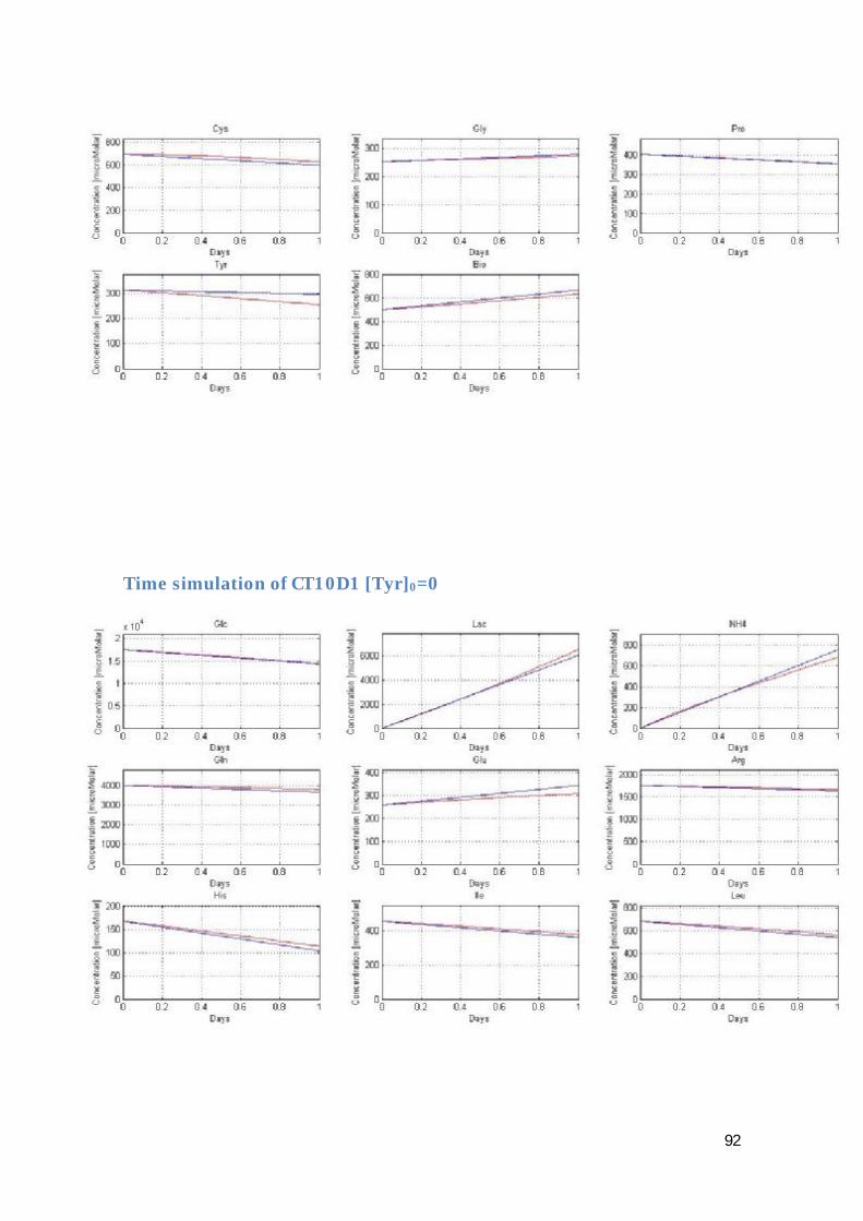
92

Time simulation of CT10D1 [Tyr]0=0

94

Time simulation of CT12D1 Reference Sample

96

Appendix VI: Function codes

calcAmac

function [Amac,EM,nmodes,externalreactions]=calcAmac(Aext,Aint,irrev) [MET,J]=size(Aext); %Calc Aem (Stoichiometric matrix of internal metabolites) and Aeem %(Stoichiometric matrix of external metabolites) ne=0; ni=0; for j=1:J if norm(Aint(:,j))==0 ne=ne+1; AeEM.ext(:,ne)=Aext(:,j); AeEM.irrev_react(ne)=irrev(:,j); externalreactions(ne)=j; else ni=ni+1; AEM.ext(:,ni)=Aext(:,j); AEM.st(:,ni)=Aint(:,j); AEM.irrev_react(ni)=irrev(:,j); end end if ne==0 AeEM.ext=0; else end

if ni==0 AEM.ext=0; AEM.st=0; AEM.irrev_react=0; else end %Calc internal elementary modes using metatool AEM= metatool(AEM); AEM.ems= AEM.sub' * AEM.rd_ems; %Calc macro reactions of the internal elementary modes AmacEM=AEM.ext*AEM.ems; [aux,numbermodesi]=size(AmacEM); %Calc number of external irrev reaction nei=0; for j=1:ne if AeEM.irrev_react(j)==0 nei=nei+1; else end end %Calc external elementary modes AeEM.ems=zeros(ne,nei+ne); eem=0; for j=1:ne eem=eem+1; AeEM.ems(j,eem)=1; if AeEM.irrev_react(j)==0;

97

eem=eem+1; AeEM.ems(j,eem)=-1; else end end %Calc macro reactions of external elem modes AmaceEM=AeEM.ext*AeEM.ems; %Calc Amac if ni==0 Amac=AmaceEM; else Amac=[AmacEM AmaceEM]; end %Calc number of EMs nmodes=numbermodesi+ne+nei; %Calc EMs from the internal and external elementary modes matrixes and set %the reactions order of the beginning if ni==0 EM=AeEM.ems; nmodes=nmodes-1; else EM=zeros(j,nmodes); nee=1; nii=1; for j=1:J if externalreactions(nee)==j EM(j,:)=[zeros(1,numbermodesi) AeEM.ems(nee,:)]; nee=nee+1; else EM(j,:)=[AEM.ems(nii,:) zeros(1,ne+nei)];

nii=nii+1; end end end

calcmus

function [MU,error]=calcmus(A,Q,C,K) [MET,J]=size(A); [MET,NS]=size(Q); %Calculate the average value for every metabolite AVERAGE=zeros(MET,1); for met=1:MET AVERAGE(met)=norm(Q(met,:),1)/J; end %Create R R=zeros(1,J*NS); %Create B B=zeros(MET*NS,J); %Calculate Qnorm Qnorm=zeros(MET,NS); for met=1:MET Qnorm(met,:)=Q(met,:)/AVERAGE(met); end %Create Qt and Ct Qt=zeros(MET*NS,1); for ns=1:NS Qt(MET*(ns-1)+1:MET*ns)=Qnorm(:,ns);

98

end Ct=zeros(MET*NS,1); for ns=1:NS Ct(MET*(ns-1)+1:MET*ns)=C(:,ns); end %Calculate B for ns=1:NS %Calculate R's such averagei*bij=aij*rij; rij=multj((S^aij/(Ki+S)^aij) for j=1:J R(j+J*(ns-1))=1; for met=1:MET if A(met,j)<0 R(j+J*(ns-1))=R(j+J*(ns-1))*Ct(met+MET*(ns-1))^(-A(met,j))/(K(met)+Ct(met+MET*(ns-1)))^(-A(met,j)); else end end end %Calculate B for met=1:MET for j=1:J B(met+MET*(ns-1),j)=R(j+J*(ns-1))*A(met,j)/AVERAGE(met); end end end

%Calculate MU using lsqnonneg %optional, if is wanted to force a starting value for the iterations: x0=0*ones(1,J); [MU,error] = lsqnonneg(B,Qt,x0); %Calculate error=norm error=sqrt(error);

calcredsys

function[Ared,MUred]=calcredsys(A,MU) [MET,NR]=size(A); %Count the number of reactions to not create variables that grow inside a %loop nrred=0; for nr=1:NR if MU(nr)==0 else nrred=nrred+1; end end %Calculate Ared and MUred MUred=zeros(nrred,1); Ared=zeros(MET,nrred); nrred=0; for nr=1:NR if MU(nr)==0 else nrred=nrred+1; Ared(:,nrred)=A(:,nr); MUred(nrred)=MU(nr); end end

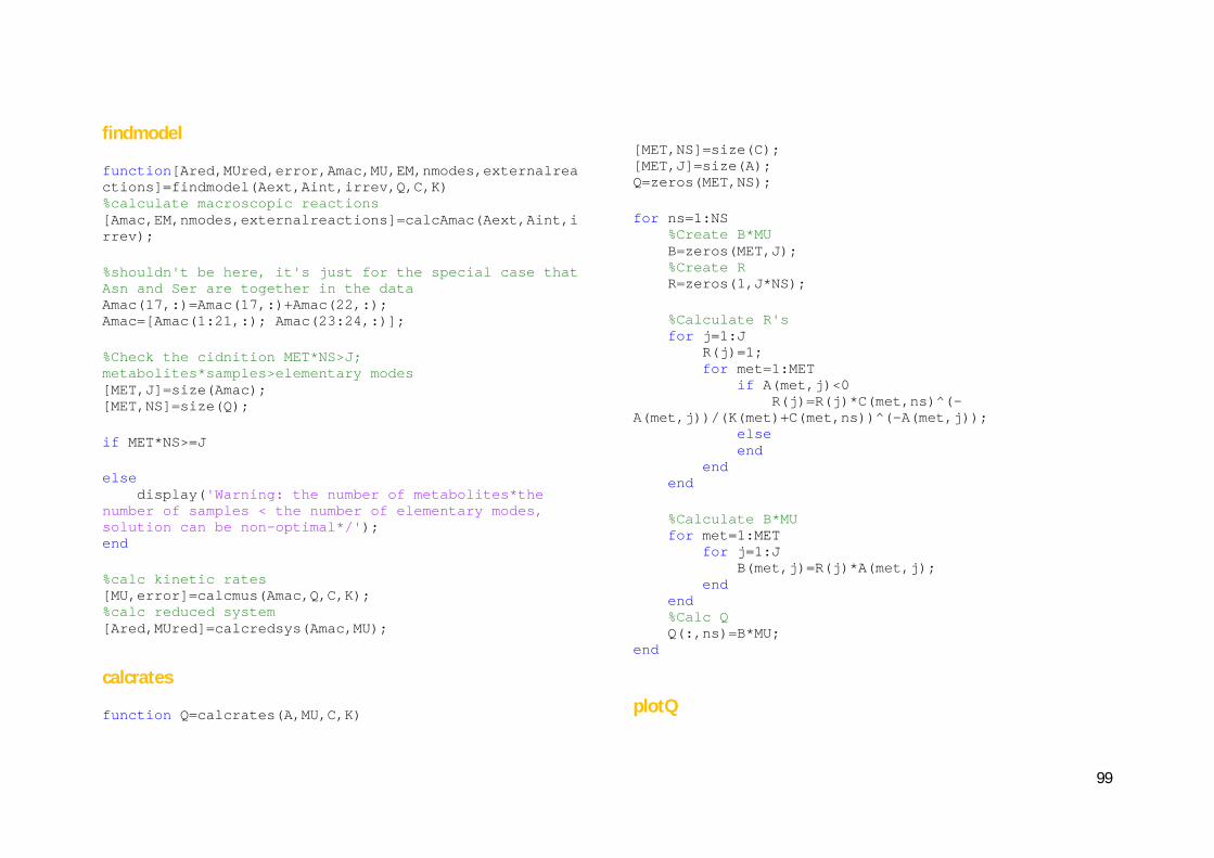
99

findmodel

function[Ared,MUred,error,Amac,MU,EM,nmodes,externalreactions]=findmodel(Aext,Aint,irrev,Q,C,K) %calculate macroscopic reactions [Amac,EM,nmodes,externalreactions]=calcAmac(Aext,Aint,irrev); %shouldn't be here, it's just for the special case that Asn and Ser are together in the data Amac(17,:)=Amac(17,:)+Amac(22,:); Amac=[Amac(1:21,:); Amac(23:24,:)]; %Check the cidnition MET*NS>J; metabolites*samples>elementary modes [MET,J]=size(Amac); [MET,NS]=size(Q); if MET*NS>=J else display('Warning: the number of metabolites*the number of samples < the number of elementary modes, solution can be non-optimal*/'); end %calc kinetic rates [MU,error]=calcmus(Amac,Q,C,K); %calc reduced system [Ared,MUred]=calcredsys(Amac,MU); calcrates

function Q=calcrates(A,MU,C,K)

[MET,NS]=size(C); [MET,J]=size(A); Q=zeros(MET,NS); for ns=1:NS %Create B*MU B=zeros(MET,J); %Create R R=zeros(1,J*NS); %Calculate R's for j=1:J R(j)=1; for met=1:MET if A(met,j)<0 R(j)=R(j)*C(met,ns)^(-A(met,j))/(K(met)+C(met,ns))^(-A(met,j)); else end end end %Calculate B*MU for met=1:MET for j=1:J B(met,j)=R(j)*A(met,j); end end %Calc Q Q(:,ns)=B*MU; end

plotQ

100

function null=plotQ(Q,Qcalc,experiments,plotcol) [MET,J]=size(Q); figure plotrows=ceil(J/plotcol); for ns=1:J subplot(plotrows,plotcol,ns) plot((1:MET),Q(:,ns),'b'); hold plot((1:MET),Qcalc(:,ns),'r'); grid on title(experiments(ns,:)); xlabel('Metabolites'); ylabel('Consumption/production [nmol/(MVC·day)]'); end null=0;

plotQ2

function null=plotQ2(Q,Qcalc,experiments,plotcol) [MET,J]=size(Q); figure plotrows=ceil(J/plotcol); for ns=1:J subplot(plotrows,plotcol,ns) plot((4:MET),Q(4:MET,ns),'b'); hold plot((4:MET),Qcalc(4:23,ns),'r'); grid on title(experiments(ns,:)); xlabel('Metabolites'); ylabel('Consumption/production [nmol/(MVC·day)]'); end null=0;

plotQnorm

function null=plotQnorm(Q,Qcalc,experiments,plotcol) [MET,J]=size(Q); AVERAGE=zeros(MET,1); %Calcualate averages for met=1:MET AVERAGE(met)=norm(Q(met,:),1)/J; end %Calcualte Qnorm Qnorm=zeros(MET,J); Qcalcnorm=zeros(MET,J); for met=1:MET Qnorm(met,:)=Q(met,:)/AVERAGE(met); Qcalcnorm(met,:)=Qcalc(met,:)/AVERAGE(met); end %Plots the calculated Qnorm's figure plotrows=ceil(J/plotcol); for ns=1:J subplot(plotrows,plotcol,ns) plot((1:MET),Qnorm(:,ns),'b'); hold plot((1:MET),Qcalcnorm(:,ns),'r'); grid on title(experiments(ns,:)); xlabel('Metabolites'); ylabel('Consumption/production'); end null=0;

101

ploterrors

function null=ploterrors(Q,Qcalc,experiments,plotcol) [MET,J]=size(Q); AVERAGE=zeros(MET,1); ERROR=zeros(MET,J); %Calcualate errors for met=1:MET AVERAGE(met)=norm(Q(met,:),1)/J; end for met=1:MET ERROR(met,:)=(Q(met,:)-Qcalc(met,:))/AVERAGE(met); end %Plot errors figure plotrows=ceil(J/plotcol); for ns=1:J subplot(plotrows,plotcol,ns) plot((1:MET),ERROR(:,ns),'b'); grid on title(experiments(ns,:)); xlabel('Metabolites'); ylabel('relative error (Q(i,ns)-Qcalc(i,ns)/average(Q(i))'); end null=0;

plotevery

function null=plotevery(Q,Qcalc,experiments,plotcol,maxplots) [MET,J]=size(Q); NP=ceil(J/maxplots);

%Plots all the figures excepting the last one for np=1:(NP-1) plotQ(Q(:,(np-1)*maxplots+1:maxplots*np),Qcalc(:,(np-1)*maxplots+1:maxplots*np),experiments((np-1)*maxplots+1:maxplots*np,:),plotcol); plotQ2(Q(:,(np-1)*maxplots+1:maxplots*np),Qcalc(:,(np-1)*maxplots+1:maxplots*np),experiments((np-1)*maxplots+1:maxplots*np,:),plotcol); plotQnorm(Q(:,(np-1)*maxplots+1:maxplots*np),Qcalc(:,(np-1)*maxplots+1:maxplots*np),experiments((np-1)*maxplots+1:maxplots*np,:),plotcol); ploterrors(Q(:,(np-1)*maxplots+1:maxplots*np),Qcalc(:,(np-1)*maxplots+1:maxplots*np),experiments((np-1)*maxplots+1:maxplots*np,:),plotcol); end %Plot the last figures which can have less graphs plotQ(Q(:,(NP-1)*maxplots+1:J),Qcalc(:,(NP-1)*maxplots+1:J),experiments((NP-1)*maxplots+1:J,:),plotcol); plotQ2(Q(:,(NP-1)*maxplots+1:J),Qcalc(:,(NP-1)*maxplots+1:J),experiments((NP-1)*maxplots+1:J,:),plotcol);

102

plotQnorm(Q(:,(NP-1)*maxplots+1:J),Qcalc(:,(NP-1)*maxplots+1:J),experiments((NP-1)*maxplots+1:J,:),plotcol); ploterrors(Q(:,(NP-1)*maxplots+1:J),Qcalc(:,(NP-1)*maxplots+1:J),experiments((NP-1)*maxplots+1:J,:),plotcol); null=0;

plotQmet

function null=plotQmet(Q,Qcalc,metabolites,plotcol) [MET,J]=size(Q); figure plotrows=ceil(MET/plotcol); for met=1:MET subplot(plotrows,plotcol,met) plot((1:J),Q(met,:),'b'); hold plot((1:J),Qcalc(met,:),'r'); grid on title(metabolites(met,:)); xlabel('Samples'); ylabel('Consumption/production [nmol/(MVC·day)]'); YMAX=max([Q(met,:) Qcalc(met,:)]); YMIN=min([Q(met,:) Qcalc(met,:)]); if YMIN>0 AXIS([0 7 0 YMAX+YMAX*0.2]); elseif YMAX<0 AXIS([0 7 YMIN+YMIN*0.2 0]); else end end

null=0;

ploteverymet function null=ploteverymet(Q,Qcalc,metabolites,plotcol,maxplots) [MET,J]=size(Q); NP=ceil(MET/maxplots); %Plots all the figures excepting the last one for np=1:(NP-1) plotQmet(Q((np-1)*maxplots+1:maxplots*np,:),Qcalc((np-1)*maxplots+1:maxplots*np,:),metabolites((np-1)*maxplots+1:maxplots*np,:),plotcol); end %Plot the last figure which can have less graphs plotQmet(Q((NP-1)*maxplots+1:MET,:),Qcalc((NP-1)*maxplots+1:MET,:),metabolites((NP-1)*maxplots+1:MET,:),plotcol); null=0;

calctimeline

function [Ccalc,time]=calctimeline(step,days,C0,Ared,MUred,K,nbio) nmetab=length(C0); nstep=ceil(days/step); time=zeros(1,nstep+1); Ccalc=zeros(nmetab,nstep+1);

103

%Calcualtes all the steps excepting the last one using Ccalc Ccalc(:,1)=C0; for i=1:nstep-1 Qcalc=calcrates(Ared,MUred,Ccalc(:,i),K); Ccalc(:,i+1)=Ccalc(:,i)+Qcalc*Ccalc(nbio,i)*step/(1000); time(i+1)=i*step; end %Calcualtes the final step which can be shorter than step finalstep=days-time(i+1); i=i+1; Qcalc=calcrates(Ared,MUred,Ccalc(:,i),K); Ccalc(:,nstep+1)=Ccalc(:,i)+Qcalc*Ccalc(nbio,i)*finalstep/(1000); time(i+1)=time(i)+finalstep;

dynamical modelling of a metabolic reaction network

Documents