Dynamical equations for the contact line

of an evaporating sessile drop

Eliot Fried

Department of Mechanical Engineering

McGill University

Background

• Many developing and advanced technologies rely on processesinvolving evaporating sessile drops.

C

Ω

ΓLV

mt

Ω

ΓLV

m

ΓLS

θ

sin θ = m ·cos θ = m ·

• Basic modes:

Constant contact radius.

Constant contact angle.

Mixed or stick-slip.

• For sufficiently small drops, the time scales of evaporation andcontact line motion become comparable.

• Due to the absence of a reliable theory and the challenges ofmaking measurements at small length and time scales, a com-plete understanding of the mechanisms governing the variousmodes is not yet available.

NIST, January 21, 2011 1/28

Questions

1. What are the evolution equations for the contact line of an

evaporating sessile drop?

2. Are dissipative mechanisms important and, if so, under what

circumstances is coupling between those mechanisms signifi-

cant?

Theory for the liquid-vapor interface alone:

• E. Fried, A.Q. Shen & M.E. Gurtin, Theory for solvent, mo-

mentum, and energy transfer between a surfactant solution

and a vapor atmosphere, Phys. Rev. E 73 (2006), 061601.

• D.M. Anderson, P. Cermelli, E. Fried, M.E. Gurtin & G.B. Mc-

Fadden, General dynamical sharp-interface conditions for phase

transformations in viscous heat-conducting fluids, J. Fluid Mech.

501 (2007), 323–370.

NIST, January 21, 2011 2/28

Outline

• Variational description of the equilibrium of a sessile drop

• Discussion and interpretation of the variational results

• The Young–Dupre equation

• Questions concerning the variational conditions at the contactline

• Mechanical balances at the contact line

• Configurational forces

• Dynamical equations for the contact line

• Take-home points

NIST, January 21, 2011 3/28

Variational description of the equilibrium of a sessile drop

C

Ω

ΓLV

mt

Ω

ΓLV

m

ΓLS

θ

sin θ = m ·cos θ = m ·

• % . . . liquid density

• ψ . . . specific Helmholtz free-energy of liquid (relative to vapor)

• ϕ . . . specific gravitational potential-energy (gradϕ = −g)

• ψLV . . . Helmholtz free-energy density of liquid-vapor interface

• ψLS . . . Helmholtz free-energy density of liquid-solid interface

• ψSV . . . Helmholtz free-energy density of solid-vapor interface

• ψC . . . Helmholtz free-energy density of contact line

NIST, January 21, 2011 4/28

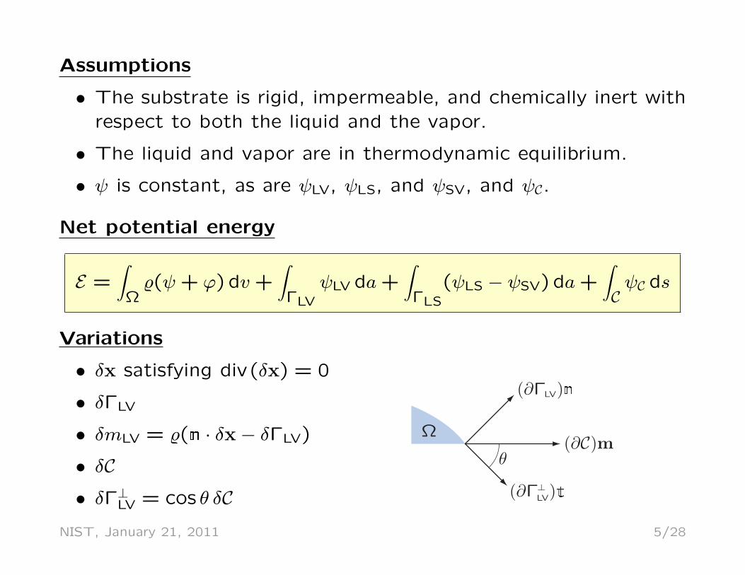
Assumptions

• The substrate is rigid, impermeable, and chemically inert withrespect to both the liquid and the vapor.

• The liquid and vapor are in thermodynamic equilibrium.

• ψ is constant, as are ψLV, ψLS, and ψSV, and ψC.

Net potential energy

E =∫

Ω%(ψ + ϕ) dv +

∫ΓLV

ψLV da+∫

ΓLS

(ψLS − ψSV) da+∫CψC ds

Variations

• δx satisfying div(δx) = 0

• δΓLV

• δmLV = %(n · δx− δΓLV)

• δC

• δΓ⊥LV = cos θ δC

Ω

θ

(∂ΓLV)

(∂C)m

(∂Γ⊥LV)

NIST, January 21, 2011 5/28

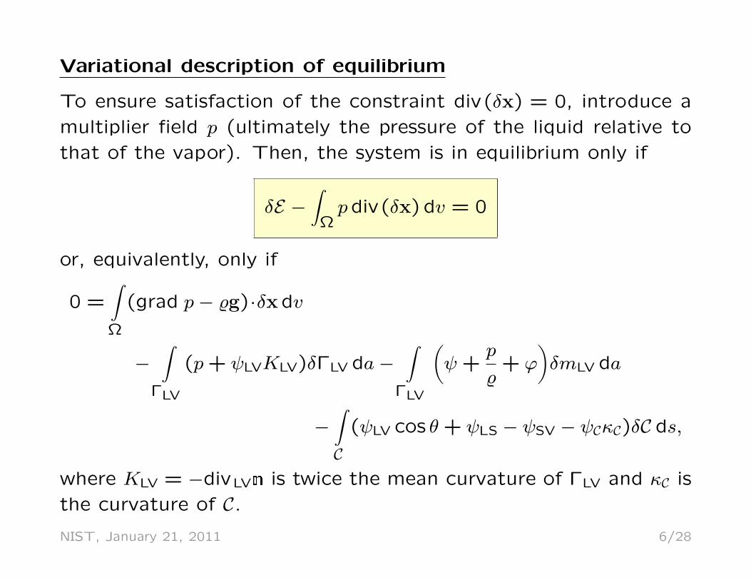
Variational description of equilibrium

To ensure satisfaction of the constraint div(δx) = 0, introduce a

multiplier field p (ultimately the pressure of the liquid relative to

that of the vapor). Then, the system is in equilibrium only if

δE −∫

Ωpdiv(δx) dv = 0

or, equivalently, only if

0 =∫Ω

(grad p− %g)·δx dv

−∫

ΓLV

(p+ ψLVKLV)δΓLV da−∫

ΓLV

(ψ +

p

%+ ϕ

)δmLV da

−∫C

(ψLV cos θ + ψLS − ψSV − ψCκC)δC ds,

where KLV = −div LVn is twice the mean curvature of ΓLV and κC is

the curvature of C.

NIST, January 21, 2011 6/28

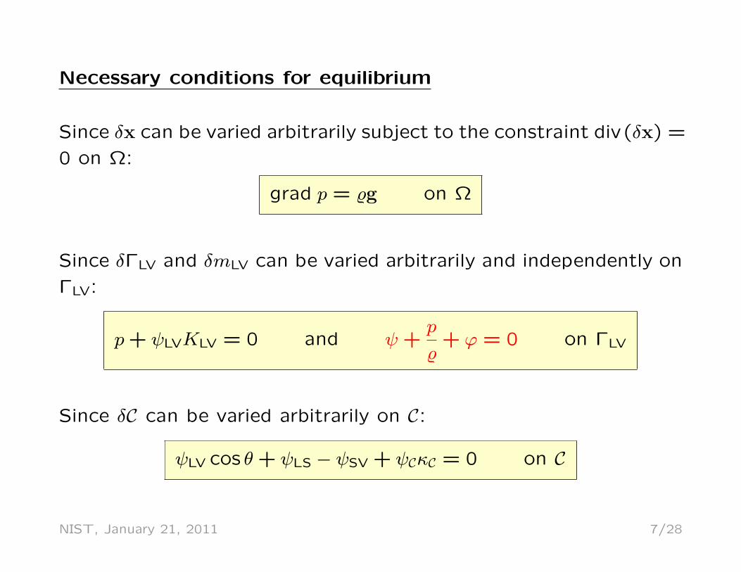
Necessary conditions for equilibrium

Since δx can be varied arbitrarily subject to the constraint div(δx) =

0 on Ω:

grad p = %g on Ω

Since δΓLV and δmLV can be varied arbitrarily and independently on

ΓLV:

p+ ψLVKLV = 0 and ψ +p

%+ ϕ = 0 on ΓLV

Since δC can be varied arbitrarily on C:

ψLV cos θ + ψLS − ψSV + ψCκC = 0 on C

NIST, January 21, 2011 7/28

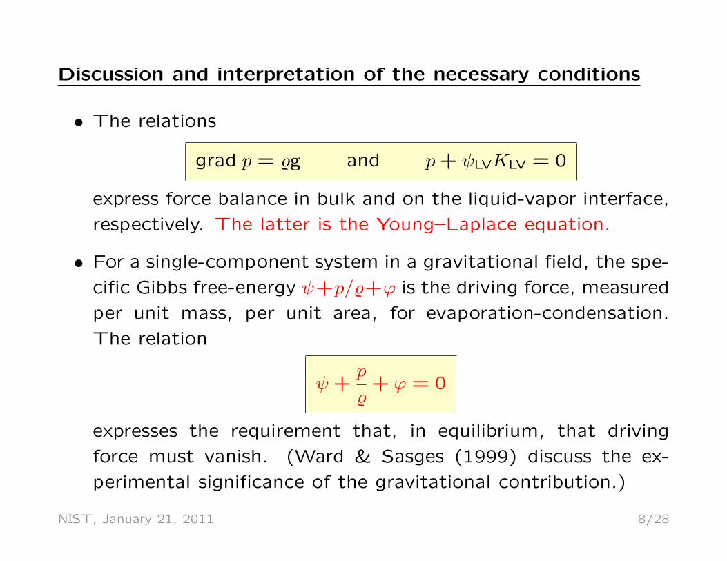
Discussion and interpretation of the necessary conditions

• The relations

grad p = %g and p+ ψLVKLV = 0

express force balance in bulk and on the liquid-vapor interface,

respectively. The latter is the Young–Laplace equation.

• For a single-component system in a gravitational field, the spe-

cific Gibbs free-energy ψ+p/%+ϕ is the driving force, measured

per unit mass, per unit area, for evaporation-condensation.

The relation

ψ +p

%+ ϕ = 0

expresses the requirement that, in equilibrium, that driving

force must vanish. (Ward & Sasges (1999) discuss the ex-

perimental significance of the gravitational contribution.)

NIST, January 21, 2011 8/28

• Eliminating p between the relations for the liquid-vapor inter-

face yields a combined balance

%(ψ + ϕ) = ψLVKLV

that can be imposed in place of the balance ψ + p/% + ϕ = 0.

This combined balance is reminiscent of the Gibbs–Thomson

condition arising in models of solidification.

• When ψC is negligible, the relation

ψLV cos θ + ψLS − ψSV − ψCκC = 0

reduces to an equation first derived by Gibbs (1878). Boruvka

& Newmann (1977) provide a substantially broader generaliza-

tion that allows the substrate to be deformable and accounts

for dependence of the various interfacial free-energy densities

on suitable strain measures.

NIST, January 21, 2011 9/28

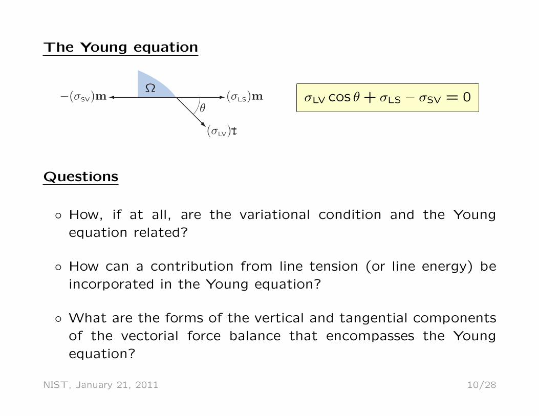
The Young equation

Ω

θ

(σLV)

(σLS)m−(σSV)m σLV cos θ + σLS − σSV = 0

Questions

How, if at all, are the variational condition and the Youngequation related?

How can a contribution from line tension (or line energy) beincorporated in the Young equation?

What are the forms of the vertical and tangential componentsof the vectorial force balance that encompasses the Youngequation?

NIST, January 21, 2011 10/28

Controversy surrounding these and other related questions is on-

going. See:

• R. Finn, Contact angle in capillarity, Phys. Fluids 18 (2006),

047102.

• I. Lunati, Young’s law and the effects of interfacial energy on

the pressure at the solid-fluid interface, Phys. Fluids 19 (2007),

118105.

• R. Finn, Comments related to my paper “The contact angle

in capillarity”, Phys. Fluids 20 (2008), 107104.

• Y.D. Shikhmurzaev, On Young’s (1805) equation and Finn’s

(2006) ‘counterexample’, Phys. Lett. A 372 (2008), 704–707.

NIST, January 21, 2011 11/28

Mechanical balances at the contact line

Suppose that:

• The liquid-vapor, liquid-solid, and solid-vapor interfaces ΓLV,ΓLS, and ΓSV are endowed with (symmetric and tangential)Cauchy stresses TLV, TLS, and TSV.

• The contact line C is endowed with Cauchy line stress τ C anda line force rCe, where e denotes the upward unit normal onthe substrate.

• The interfaces and the contact line are not sufficiently massyto warrant the inclusion of interfacial or contact-line inertia.

The linear- and angular-momentum balances for a segment L of Care then given by∫

L(TLS −TSV)m ds−

∫LTLVtds+ τ C

∣∣∣∂L

+∫LrCe ds = 0

NIST, January 21, 2011 12/28

and∫L

(x− o)× (TLS −TSV)m ds−∫L

(x− o)×TLVtds

+ (x− o)× τ C∣∣∣∂L

+∫L

(x− o)× rCe ds = 0.

• Since L is arbitrary, these balances localize to

(TLS −TSV)m−TLVt +∂τ C

∂s+ rCe = 0,

where s denotes arclength along C, and

t⊗ τ C = τ C ⊗ t.

• The latter balances implies that τ C is tangential to C:

τ C = τCt.

NIST, January 21, 2011 13/28

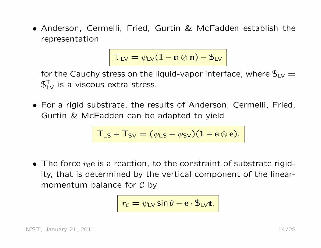
• Anderson, Cermelli, Fried, Gurtin & McFadden establish the

representation

TLV = ψLV(1− n⊗ n)− SLV

for the Cauchy stress on the liquid-vapor interface, where SLV =

S>LV is a viscous extra stress.

• For a rigid substrate, the results of Anderson, Cermelli, Fried,

Gurtin & McFadden can be adapted to yield

TLS −TSV = (ψLS − ψSV)(1− e⊗ e).

• The force rCe is a reaction, to the constraint of substrate rigid-

ity, that is determined by the vertical component of the linear-

momentum balance for C by

rC = ψLV sin θ − e · SLVt.

NIST, January 21, 2011 14/28

• In view of the Frenet relation ∂t/∂s = κCm, the linear-momentum

balance for C has normal and tangential components

ψLV cos θ −m · SLVt + ψLS − ψSV + τCκC = 0

and

t · SLVt =∂τC

∂s.

• The first of the above equations does not coincide with the

variational condition

ψLV cos θ + ψLS − ψSV + ψCκC = 0

unless m · SLVt = 0 and τC = ψC.

• If ψC = τC = 0, then the variational condition and the Young

equation coincide.

NIST, January 21, 2011 15/28

Observations

This approach resolves:

• Issues concerning balances normal to the substrate and tan-gential to the contact line.

• The connection between the interfacial tensions and the inter-facial energies: σLV = ψLV + trSLV

Additional questions

• Why does the variational approach yield two equilibrium con-ditions on the liquid-vapor interface but only a single conditionat the contact line?

• Does τC = ψC in equilibrium?

• Does a single balance suffice away from equilibrium?

NIST, January 21, 2011 16/28

Digression: Configurational forces

Sixty years ago, solid state physicists and materials scientists began

to promote the view that the forces governing the arangement of

defects in crystalline solids are distinct from the Newtonian forces

that are classically associated with the motion of atoms. These

nonstandard forces are nowadays called configurational.

• M.O. Peach & J.S. Koehler, The forces exerted on dislocations

and the stress fields produced by them, Phys. Rev. 80 (1950),

436–439.

• J.D. Eshelby, The force on an elastic singularity, Phil. Trans.

R. Soc. A 244 (1951), 87–112.

• C. Herring, Surface tension as a motivation for sintering, in

The Physics of Powder Metallurgy (W.E. Kingston, ed.), Mc-

Graw-Hill, New York, 1951.

• W.W. Mullins, Two-dimensional motion of idealized grain bound-

aries, J. Appl. Phys. 27 (1956), 900–904.

NIST, January 21, 2011 17/28

• Configurational forces act over nonmaterial entities, such as:

Vacancies, substitutional impurities, interstitial impurities

Dislocations, disclinations

NIST, January 21, 2011 18/28

Grain boundaries, twin boundaries, phase interfaces

• Defects move relative to the underlying material

and, thus, involve kinematical descriptors and power-conjugate

pairings that are distinct from those associated with the motion

of the material.

NIST, January 21, 2011 19/28

How are configurational forces characterized?

• The early workers relied exclusively on variational arguments.

• This approach persisted until nearly two decages ago at whichpoint Gurtin began developing an approach designed to de-scribe dynamical processes involving dissipation.

• Gurtin’s program involves:

Introducing configurational forces as primitive quantities sub-ject to a balance distinct from those governing standardNewtonian forces.

Accounting properly for all power expenditures and usingthe second law of thermodynamics to obtain constitutiverestrictions on configurational forces.

• The program has been applied successfully to develop theoriesfor various classes of phase transformations, including mostrecently evaporation-condensation processes in fluids—whereviscous dissipation is of prominent importance.

NIST, January 21, 2011 20/28

Treatment of the contact line

For a segment L of C, the configurational momentum balance isimposed in the form∫

L(CLS − CSV)m ds−

∫LCLVtds+ cC

∣∣∣∂L

+∫L

fC ds = 0,

where:

• CLV, CLS, and CSV are interfacial configurational stresses anal-ogous to the interfacial Cauchy stresses TLV, TLS, and TSV.However, they needn’t be symmetric.

• cC is a configurational line tension analogous to τ C. However,it needn’t be tangential.

• fC is an internal configurational line force.

The configurational balance should be compared with the mechan-ical balance∫

L(TLS −TSV)m ds−

∫LTLVtds+ τ C

∣∣∣∂L

+∫LrCe ds = 0.

NIST, January 21, 2011 21/28

The final, intrinsic form of the free-energy inequality for a segment

L of C is

d

dt

∫LψC ds ≤ −

∫LfCV

migC ds+

∫LτCm ·

∂u

∂sds

+∫LξC∂V migC∂s

ds−∫LψCκCV

migC ds+ ψCV

migC |∂L,

where:

• V migC is the component of the velocity of C in the direction of

m relative to the component u ·m of the fluid velocity u at Cin the direction of m.

• ξC = cC ·m is the normal component of the configurational line

stress cC (which is analogous to the Cauchy line stress τ C).

• fC = fC ·m is the normal component of the internal configura-

tional force fC.

NIST, January 21, 2011 22/28

General contact line equations

Normal component of the linear-momentum balance:

ψLV cos θ + m · SLVt + ψLS − ψSV − τCκC = 0

Tangential component of the linear-momentum balance:

t · SLVt +∂τC

∂s= 0

Normal component of the configurational-momentum balance:

ψLV cos θ + ψLS − ψSV − ψCκC +∂ψC

∂scos θ

− ξCκC cos θ +∂ξC

∂s+ cLV · t = fC

NIST, January 21, 2011 23/28

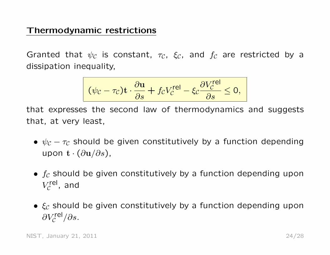
Thermodynamic restrictions

Granted that ψC is constant, τC, ξC, and fC are restricted by a

dissipation inequality,

(ψC − τC)t ·∂u

∂s+ fCV

relC − ξC

∂V relC∂s

≤ 0,

that expresses the second law of thermodynamics and suggests

that, at very least,

• ψC − τC should be given constitutively by a function depending

upon t · (∂u/∂s),

• fC should be given constitutively by a function depending upon

V relC , and

• ξC should be given constitutively by a function depending upon

∂V relC /∂s.

NIST, January 21, 2011 24/28

Allowing for linear, coupled dissipative mechanisms yields

ψC − τC = −γ11t ·∂u

∂s− γ12V

relC − γ13

∂V relC∂s

,

fC = −γ21t ·∂u

∂s− γ22V

relC − γ23

∂V relC∂s

,

−ξC = −γ31t ·∂u

∂s− γ23V

relC − γ33

∂V relC∂s

,

where the matrix γ11 γ12 γ13γ12 γ22 γ23γ12 γ23 γ33

of contact-line viscosities is positive semidefinite.

Questions

1. Are dissipative mechanisms important and, if so, is coupling

between those mechanisms significant?

2. Can we design experiments to accurately measure the contact-

line viscosities? Contact-line rheometry???NIST, January 21, 2011 25/28

Other questions for contact lines

• Why does the variational approach yield two equilibrium con-ditions on the liquid-vapor interface but only a single conditionat the contact line?

• Does τC = ψC in equilibrium?

• Does a single balance suffice away from equilibrium?

Answers

• In equilibrium, unless the interface and contact line are massy,there is no analog of the driving force ψ+p/%+ϕ and the nor-mal components of the linear- and configurational-momentumbalances for C coalesce.

• In general, τC = ψC + σC, where σC is dissipative.

• Away from equilibrium, the normal component of the config-urational-momentum balance on the contact line is not redun-dant. It governs the kinetics of contact line motion.

NIST, January 21, 2011 26/28

Connection with previous contact line conditions

• When dissipative effects are neglected, the balances for thecontact line C reduce to a single balance

ψLV cos θ + ψLS − ψSV − ψCκC +∂ψC

∂scos θ = 0.

This equation was derived by Boruvka & Newmann (1977)using variational means. More recently, it was rediscoveredby Swain & Lipowsky (1998) and Schimmele, Napiorkowski &Dietrich (2007).

• In a very early attempt to explain observed hysteretic behaviorof a contact line, Adam & Jessop (1925) used

ψLV cos θ + ψLS − ψSV = f,

with f depending on the contact line velocity but not neces-sarily in a way that would ensure satisfaction of the second lawof thermodynamics.

NIST, January 21, 2011 27/28

Take-home points

• Away from equilibrium,

the Young equation is replaced by an equation expressinglinear-momentum balance, and

the configurational-momentum balance yields an additional,independent equation for the kinetics of contact line motion.

• At equilibrium,

the additional, independent equation for the contact line issatisfied trivially, and

the variational condition for the contact line and the Youngequation coincide.

• Configurational forces arise and are important not only to lat-tice defects, but also to phase transformations in fluids.

• Analysis of the full system of equations for an evaporating dropis in progress. Experiments are also being designed.

• Questions regarding the role/importance of dissipative mech-anisms at contact lines remain unaddressed. . .

NIST, January 21, 2011 28/28